Embed Size (px)
Citation preview

University of Southern Queensland Faculty of Engineering and Surveying
DESIGN AND TRIAL OF AN ALTERNATIVE OPTION FOR
SUBURBAN SEWERAGE PUMP STATIONS
A dissertation submitted by
Bill Thomas Weston
in fulfilment of the requirements of
Courses ENG4111 and ENG4112 Research Project
towards the degree of
Bachelor of Engineering (Mechanical Engineering)
Submitted October 2007

i
Abstract Collection and pumping of waste water represents a significant cost for urban communities in Australia. The flows in a sewerage system are not constant. In residential areas flows will be at a maximum in the morning and evening. Additionally during rain periods there is an increase of flow into the pump stations due to faults in the gravity sewers allowing inflows and infiltration. It is common for multiple pump stations to feed into the same pressure main. This causes the pressure in the common pressure main to change depending on how many and which pumps are operating at any given time. Consequently the pump stations feeding into the common pressure main will operate at various flows. A given pump station will operate against maximum pressure during wet weather when all other pump stations are also operating, resulting in a decrease in the flow rate produced by the pump station. This is not desirable as the largest flow outputs are needed during wet weather conditions. The purpose of this project is to devise an alternative pump configuration. The configuration will enable pumps to operate within their recommended operating range for normal and wet weather operating conditions. The design must comply with the current standards required by the waste water industry. It must also be cost competitive compared with current pump station designs, and be able to be operated and maintained effectively in a similar manner to existing designs. The selected pump configuration consisted of three identical pumps. For normal dry weather operation each pump operates as a stand alone unit (i.e., duty / standby / standby). The pumps are equipped with piping and valving to enable two pumps to operate in series to deliver the higher pressures needed during wet weather operation. (i.e., duty / duty / standby). A prototype of this series pump configuration was designed and built. The prototype was run in a test tank to compare measured and theoretical pump performance. The tests undertaken in the test tank indicated that the pump configuration performed as predicted and it was therefore suitable for installation in an operating sewerage pump station. The prototype pumps were installed in an existing sewerage pump station in July 2007. Monitoring of the performance showed that the pumps successfully operated within their recommended operating range for normal dry weather operation and for simulated wet weather operation. There has been no evidence of increased susceptibility to blockage with this pump configuration. The proposed series pump arrangement appears to meet the goal of providing a cost effective alternative that uses identical fixed speed pumps. Each pump operates within the recommended range above and below the best efficiency point under all flow conditions. Longer term field testing is needed to demonstrate satisfactory reliability and performance of the pumps over an extended period.

ii
University of Southern Queensland
Faculty of Engineering and Surveying
ENG4111 and ENG4112 Research Project
Limitations of Use The Council of the University of Southern Queensland, its Faculty of
Engineering and Surveying, and the staff of the University of Southern
Queensland, do not accept any responsibility for the truth, accuracy or
completeness of material contained within or associated with this dissertation.
Persons using all or any part of this material do so at their own risk, and not at
the risk of the Council of the University of Southern Queensland, its Faculty of
Engineering and Surveying or the staff of the University of Southern
Queensland.
This dissertation reports an educational exercise and has no purpose or validity
beyond this exercise. The sole purpose of the course "Project and Dissertation"
is to contribute to the overall education within the student’s chosen degree
programme. This document, the associated hardware, software, drawings, and
other material set out in the associated appendices should not be used for any
other purpose: if they are so used, it is entirely at the risk of the user.
Professor Frank Bullen
Dean
Faculty of Engineering and Surveying

iii
Certification
I certify that the ideas, designs and experimental work, results, analyses and
conclusions set out in this dissertation are entirely my own effort, except where
otherwise indicated and acknowledged.
I further certify that the work is original and has not been previously submitted
for assessment in any other course or institution, except where specifically
stated.
Bill Thomas Weston
Student Number: 0011220292
Signature
Sunday, 28 October 2007 Date

iv
Acknowledgments
This research project was initially carried out under the supervision of Dr. Ruth
Mossad, and completed with the supervision of Dr. Ahmad Sharifian. Dr.
Jonathan Harris provided supporting supervision locally. The author would like
to thank Dr. Mossad for her encouragement and provision of ideas throughout
the project specification and literature review process. Dr. Sharifian should also
be acknowledged for accepting the role as supervisor at short notice, providing
positive support and as a source of technical knowledge. The author would also
like to thank Dr. Harris for giving up many hours of his personal time to help
with this project, as well as much needed support and advice.
Acknowledgement must also go the project sponsor Citiwater Townsville.
Without the financial support, access to their facilities and personnel, this
project would not have been able to be undertaken. People that deserve special
thanks include Vivek Kangesu and Grant Brinkman for their initial support and
encouragement when the series pump configuration was a concept comprising
of sketches on a whiteboard, Kevin McGrath and Mario DeJong for drafting,
engineering advice and ensuring the pumps were installed in time for this paper
to be completed. Finally, Lachlan Thomson and Matthew Wilkie for providing
information and all the operating data and Darrel Davies and his entire crew for
putting up with my requests and helping out whenever I needed it.
I would also like to thank my wife and daughter for their help and tolerance in
the final weeks while collating this dissertation.
v
Table of Contents
Chapter 1: Introduction ......................................................................................... 1
1.1 Background ................................................................................................... 1
1.2 Problem Identification.................................................................................. 3
1.3 Research Objectives...................................................................................... 5
Chapter 2: Literature Review................................................................................ 6
2.1 Pump Station Requirements ........................................................................ 6
2.2 Pump Operation and Selection.................................................................... 7
2.2.1 Best Efficiency Point ............................................................................... 8
2.2.2 Cavitation............................................................................................... 10
2.2.3 Recommended Operating Range ........................................................... 11
2.3 Pump Station Configuration Options ....................................................... 12
2.3.1 Current Citiwater Method...................................................................... 13
2.3.2 Variable Frequency Drive...................................................................... 15
2.3.3 Parallel Operation .................................................................................. 16
2.3.4 Series Operation..................................................................................... 17
2.3.5 Summary................................................................................................ 20
2.4 Conclusions: Chapter 2 .............................................................................. 20
Chapter 3: Prototype Design ............................................................................... 22
3.1 Design Process ............................................................................................. 22
3.2 Design Considerations ................................................................................ 23
3.3 Component Design...................................................................................... 23
3.3.1 Under pump valve.................................................................................. 24
3.3.2 Auto Couple Design............................................................................... 24
3.3.3 Pump Casing Pressure Rating................................................................ 27
3.3.4 Materials ................................................................................................ 27
3.4 Model Calculations ..................................................................................... 28
Chapter 4: Prototype Testing .............................................................................. 30
4.1 Flow and Pressure measurement............................................................... 31

vi
4.2 Test Tank Results........................................................................................ 33
4.2.1 Pump 1 Performance.............................................................................. 34
4.2.2 Pump 2 Performance.............................................................................. 35
4.2.3 Both Pumps Operating Performance ..................................................... 37
4.3 Flows through Standby Pump ................................................................... 38
Chapter 5: Operation in Pump Station............................................................... 41
5.1 Pump Control Method................................................................................ 41
5.2 Dry Weather Operation ............................................................................. 43
5.3 Simulated Wet Weather Operation........................................................... 46
5.4 Resistance to Blockage................................................................................ 48
5.5 Summary of Operational Testing.............................................................. 48
Chapter 6: Conclusions ........................................................................................ 49
6.1 Pump Station Configurations .................................................................... 49
6.2 Series Pump Configuration Suitability ..................................................... 49
6.3 Recommendations....................................................................................... 51
6.4 Further Work.............................................................................................. 51
References.............................................................................................................. 52
Appendices............................................................................................................. 54
vii
List of Figures
1.1 Example Flow-Head performance curve for Centrifugal pump…....….2
1.2 Pump station resistance curve courtesy of Citiwater Townsville…….3
1.3 Pump station resistance curve with current method of pump selection...4
2.1 Centrifugal pump performance curve………………..……….….…....8
2.2 Radial forces on pump shaft…………………………….…….….…...9
2.3 Recommended operating range for centrifugal pumps…………....…11
2.4 System resistance curve for Pump Station A11B………………….….12
2.5 Pumps for Pump Station A11B selected using current method…..…13
2.6 Pumps for Pump Station A11B selected using VFD method…………15
2.7 Schematic representation of pumps operating in parallel…….…....16
2.8 Pump Station A11B with pumps in parallel…………………….…...16
2.9 Schematic representation of pumps operating in series………..…….17
2.10 Pump Station A11B with pumps in series…………………………...17
2.11 Pump configuration to operate in series or singularly…………….…18
2.12 Pump arrangement for pumps to operate in series or singularly…….19
3.1 Design process flow diagram………….……………………….…….22
3.2 Under pump valve details…………………………………..………..24
3.3 Submersible pump being lowered onto pedestal………………………25
3.4 Final prototype design showing key design features………………..26
3.4 Performance estimates after pumps have been modified……………...29
4.1 Prototype pumps installed in test tank………………………….……30
4.2 Schematic of test tank showing……………………………………...31
4.3 Arrangement of pressure gauge………………………………….…..32
4.4 Differential pressure gauge and …………………………………......33
4.5 Manufacturer’s head flow curve with test results……………...…….35
4.6 Manufacturer’s head flow curve with test results for pump 2…….…36
4.7 Head flow curve for Pump 1 + Pump 2……………………………...38
4.8 Loss coefficient K2-4 estimation………………………………..……...40

viii
5.1 Schematic of pump start and stop levels…………………….……….41
5.2 Pump station flow rate pump station over single day…………………43
5.3 Pump station outflow and pressure during low flow period………...44
5.4 Pump station outflow and pressure during peak flow time………….45
5.5 Pump station outflow over twelve days……………………………...45
5.6 Pump station during simulated wet weather flow conditions……..…..47
List of Tables
2.1 Comparison of pump configuration options………………..…..……20
3.1 Material use summary………………………………………………..27
4.1 Test results for Pump 1……………………………………………....34
4.2 Test results for Pump 2………………………………………………35
4.3 Test results for Pumps 1 and 2 operating at the same time………….37
4.4 Flow rate thorough non operating pump 2 with pump 1 running……38
4.5 Loss coefficient for connecting pipework……………….…………..39
4.6 Flows thorough pump 1 when not operating ………………….………40
5.1 Initial control level for pumps……………………………...………..42
5.2 Operating statistics for prototype pumps…………………..………….48

ix
List of Appendices
Appendix A Project Specification ................................................................... 55
Appendix B Risk Assessment........................................................................... 56
Appendix C Loads on Auto Couple................................................................. 58
Appendix D Prototype Drawings..................................................................... 61
Drawing No. CC316-01; Sewage – Garbutt Pump Station A11B Series
Pump Trial, General Arrangement
Drawing No. CC316-02; Sewage – Garbutt Pump Station A11B Series
Pump Trial, Support Frame
Drawing No. CC316-03; Sewage – Garbutt Pump Station A11B Series
Pump Trial, Manifold Details
Drawing No. CC316-04; Sewage – Garbutt Pump Station A11B Series
Pump Trial, Discharge Manifold Details
Drawing No. CC316-05; Sewage – Garbutt Pump Station A11B Series
Pump Trial, Items
Appendix E, Manufactures Specifications...................................................... 67
Grundfos SV034DHU50 pump specifications
AVK FLEXI CHECK VALVE PN 16, brochure
Tyco Flow ControlRubber Expansion Joints – Type FSF, brochure
Tyco Water Resilient Seated gate Valves – Figure 500, brochure
Appendix F Friction Loss Calculations .......................................................... 79

1
Chapter 1: Introduction “The average rate payer has little concept of the size and complexity of our sewer
network, as long as it disappears when they press the button they are happy”
Retired sewerage engineer.
“Cost saving in design and construction can deliver major benefits. Sewage
collection systems account for $16.23 billion of the total $20.4 billion current
replacement cost of sewerage assets.”
Dr John Langford,
Former Executive Director of Water Services Association of Australia
1.1 Background
Typical waste water collection systems consist of a network of gravity sewers to
remove waste water from the point where it is generated. Ideally the waste water
is transported to treatment plants by gravity, when this is not possible pump
stations are used. Sewage pump stations have two basic hydraulic configurations,
the pumps either discharge directly into a gravity sewer or into a pressure main.
The flows in a sewerage system are not constant. In residential areas flows will be
at a maximum in the morning and evening and reduce to a minimum overnight
and during the day. Additionally during rain periods there is an increase in inflow
into the pump stations due to faults in the gravity sewers. These faults could be
age related, such as cracks caused by tree roots or movement of soil, and also
present in new pipes due to incorrectly fitted joints. To prevent pump stations
from overflowing the pumps must be able to operate with higher flows than the
incoming flow in both wet and dry weather. The flow rate that a pump operates at
is termed the duty point.
The most common type of pump used in sewerage pumping stations is a
centrifugal pump. The pressure developed by a centrifugal pump depends on the
volume flow rate of fluid that is passing through it. At low flow rates the pump
will develop a large pressure difference between the inlet and outlet and at high
flow rates a lower pressure difference is generated. The performance of individual

2
pumps is displayed on a pump performance curve which can be obtained from the
pump manufacturer. Pump curves are normally provided for pure water and
adjustments may be needed to account for fluids with significantly different
density, viscosity or solids contents. The pressure is displayed as head in metres
of water. As well as head (pressure), performance curves also show other
information such as pump efficiency and input power as functions of flow rate.
An example pump performance curve showing head versus flow rate is shown in
figure 1.1. This is sometimes referred as the Flow-Head performance curve.
Pump Performance Curve
0
5
10
15
20
25
30
0 10 20 30 40
Flow (l/s)
Hea
d (m
)
Figure 1.1 Example Flow-Head performance curve for Centrifugal pump.
Pump stations that discharge into a gravity sewer are called lifting stations. In this
situation the system resistance curve remains essentially unchanged for dry or wet
weather flows. Accordingly each pump operates over a very narrow range of flow
rates as the system resistance remains essentially constant. This simplifies pump
selection and this type of station will not be discussed further.
Often pump stations discharge directly into a pressure main and it is common for
multiple pump stations to feed into the same main. The flow rate and pressure in
the receiving pressure main can vary significantly depending on how many and
which pump stations are operating at any given time. The changing flow though
the main results in a changing pressure at each individual pump station.

3
Consequently the pumps in this type of station will operate over a considerable
range of duty points. The pump station will usually operate at maximum pressure
during wet weather when all other pump stations that discharge into the common
pressure main are operating simultaneously.
1.2 Problem Identification
To enable the duty points of pumps to be determined system resistance curves are
produced. For complex pressure main systems with a number of pump stations
and possible flow paths the system resistance curve varies depending on how
many other pumps stations are operating, and hydraulic analysis computer
programs such as WaterCAD are used to determine the range of system resistance
curves.
The operating flow rate requirements are either calculated from estimated
population of the catchment or by taking flow records over a period of time.
Example system resistance curves for a pump station discharging into a pressure
main are shown in figure 1.2 Note the system curve for wet weather conditions
represents the maximum system resistance, whereas the system curve for
minimum dry weather conditions represents the minimum system resistance. In
practice the system resistance can lie anywhere within these bounds.
Typical Pump Station Resistance Curve
Minimum Dry Weather Duty Point
Required Wet Weather Duty Point
Flow (l/s)
Hea
d (m
)
Minimum Dry WeatherFlow Conditions
Average Dry WeatherFlow Conditions
Wet Weather FlowConditions
Figure 1.2 Pump station resistance curve courtesy of Citiwater Townsville.

4
For small and medium sized pump stations (flows less then 200 l/s) discharging
into pressure mains the current design method used by Citiwater Townsville is to
equip the pump stations with two constant speed pumps of different sizes. A small
pump is installed to operate during normal dry weather conditions, and this pump
operates the majority of the time. The small pump is sized to be able to handle the
daily peak flows and is controlled by a level sensor in the wet well. For the station
to be able to continue operating during the high demand rain periods a larger “wet
weather” pump is also installed. The same resistance curve with the Flow-Head
performance curves for these pumps is shown in figure 1.3. The flow rate
achieved by each pump will be at the point where the resistance curve intersects
with the respective Flow-Head performance curve.
Typical Pump Station Resistance Curve
Minimum Dry Weather Duty Point
Required Wet Weather Duty Point
Flow (l/s)
Hea
d (m
)
Minimum Dry WeatherFlow ConditionsAverage Dry WeatherFlow ConditionsWet Weather FlowConditions
Dry Weather PumpPerformance CurveWet Weather PumpPerformance Curve
Figure 1.3 Pump station resistance curve with current method of pump selection.
If the small pump fails the larger wet weather pump automatically operates as a
backup pump. The large pump is run intermittently through the dry season to
prevent a build up of solids internally and to ensure it will run when it rains.
Problems observed with this configuration include;
1. The larger wet weather pump is required to operate over a wide range of
its performance curve. There is a high likelihood it will operate outside
its recommended operating range (see section 2.2).

5
2. When the large pump runs as a standby pump the larger flows it produces
will increase pressure in the discharge pressure main. In turn this will
reduce the output of other pump stations in the system.
3. If the large pump fails during a rain event there is no backup pump
capable of handling the wet weather flows. This could cause overflows of
raw sewerage to the environment or into people’s properties.
4. The purchase and installation cost of the large pump is generally more
than double the cost for the small pump. This includes the cost of heavier
electric cabling, switchboard components and larger piping.
5. Cost of maintaining the larger pump is higher due to the size of
components.
6. The number of spare parts needed is doubled by having two different
sized pumps in each station. This also increases the number of pump
sizes used over the whole sewer system, making interchange of
components between pump stations more difficult.
1.3 Research Objectives
This project will seek to provide an alternative pump configuration that will
eliminate or reduce the problems identified above. This configuration must enable
pumps to function within their preferred operating range for different system
resistance curves caused by varying demand. The design must also comply with
the current standards required by the waste water industry.
To carry out this investigation the author approached Citiwater Townsville for a
suitable location to enable testing to be done in a sewerage pump station.
Citiwater made pump station A11B available which was due for refurbishment in
the 2006-2007 financial year.

6
Chapter 2: Literature Review The literature review consists of three parts; firstly, an overview of the
requirements to satisfy current industry standards in respect to pump sizing and
configuration; secondly an investigation of the recommendations of operating
ranges for centrifugal pumps; and lastly research into different pump
configurations and their suitability for this application.
2.1 Pump Station Requirements
The Water Services Association of Australia (WSA) jointly with Standards
Australia publishes a series of design codes for the operation of water and waste
water infrastructure. The Sewerage Code of Australia requires a sewerage system
to be able to convey a design flow. The design flow is the total of the peak daily
dry weather flow (normal sewerage), with any flows from groundwater infiltration
and the peak rainfall inflow (WSA 2002 p.52). To comply with this code
Citiwater specify that pump stations must be able to convey a minimum of five
times Average Dry Weather Flow (ADWF) under wet weather flow conditions
(Citiwater 2004 pp.E-9 – E-10).
Citiwater also specify a duty point for dry weather flows as 2 x ADWF (Citiwater
2004 p. E-9) under average dry weather flow conditions. In practice this duty
point is not used by operational staff (Davies D 2007, pers. comm., April 4), as
they prefer the pumps to run a maximum of 5 hours a day under dry flow
conditions (i.e. 4.8 x ADWF). Some of the reasons given for this preferred higher
flow rate during dry weather are:
- During peak flow periods the output of the pump station is equal to or less
than the inflow which can cause a build up of fats and oils
- Pumps operating for 12 hours a day will have increased rates a wear
resulting in decreased performance.
- Allows for longer service intervals.
It is a requirement that the failure of any one piece of equipment will not prevent
the pump station from operating (WSA 2005 p.54). Therefore pump stations
normally have a minimum of two pumps installed (Citiwater 2004 p. E-9). As

7
many of Citiwater’s stations pump directly into a common pressure, pumps of
different sizes are commonly used in a single pump station to achieve a wider
range of flows as mentioned above. Sanks recommends the use a single pump size
to reduce the number of spares and allow pumps to be interchangeable (Sanks
1989 p. 318). To enable peak demand to be met multiple pumps may be run
simultaneously. In some cases the waste water authority may specify that only
identical pumps must be installed in a station (Goulburn Valley Water 2007 p. 2).
Installing identical “duty / standby” pumps, each provided with a variable speed
drive, is another option for using a single pump size whilst covering a range of dry
and wet weather flows. However, variable speed drives are considerably more
expensive than fixed speed drives, which is a disadvantage of this approach.
To reduce the impact of noise in residential areas, small and medium sized pump
stations (pumping capacity < 200 l/s) should be of a single well design (Citiwater
2004 p. E-8) and use submersible pumps. The maximum operating speed of the
pump is normally 1500 rpm (WSA 2005 p.90), although higher speeds may be
used with permission of the local authority. Other advantages of submersible
pumps include lower construction cost as no building or dry wells are needed to
house pumps (Sanks 1989 p. 774), less land use and pumps are self priming. The
use of guide rails and auto coupling pump stands mean that service personnel do
not need to enter a confined space to service pumps.
Pump Stations would satisfy the requirements recommended by WSA and Sanks
if
1. The pumps installed could provide greater than 5 x ADWF in both normal
and wet weather flow conditions
2. There are standby pumps for both normal and wet weather flow conditions
3. The pumps are of a submersible design operated at less than 1500 rpm and
if possible the pumps are the same model.
2.2 Pump Operation and Selection
Pumps may be classified as either positive displacement or kinetic (Sanks 1989
pp.277 – 279). Note some texts refer to kinetic pumps as dynamic (Fox,
McDonald & Pritchard 2004, p. 487) and in relation to pumps these terms are
8
interchangeable. Positive displacement pumps due to their complexity and higher
costs are rarely used (Sanks 1989 p. 309) in sewerage pump stations (except in
high head applications) and will not be discussed further. The most common type
of kinetic pump is the centrifugal pump, and is defined by Astall & Rogers as “a
machine that moves liquid by accelerating it radially outward in a rotating
impeller to a surrounding stationary housing”.
2.2.1 Best Efficiency Point
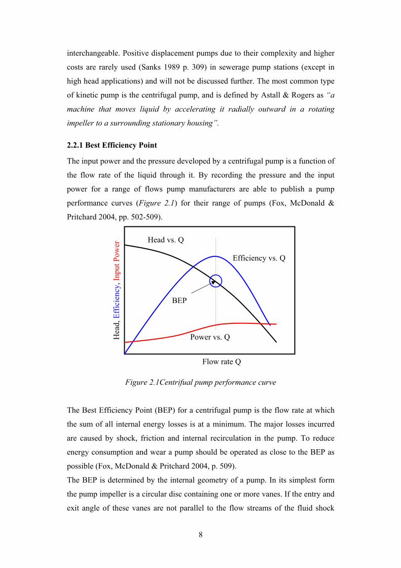
The input power and the pressure developed by a centrifugal pump is a function of
the flow rate of the liquid through it. By recording the pressure and the input
power for a range of flows pump manufacturers are able to publish a pump
performance curves (Figure 2.1) for their range of pumps (Fox, McDonald &
Pritchard 2004, pp. 502-509).
Figure 2.1Centrifual pump performance curve
The Best Efficiency Point (BEP) for a centrifugal pump is the flow rate at which
the sum of all internal energy losses is at a minimum. The major losses incurred
are caused by shock, friction and internal recirculation in the pump. To reduce
energy consumption and wear a pump should be operated as close to the BEP as
possible (Fox, McDonald & Pritchard 2004, p. 509).
The BEP is determined by the internal geometry of a pump. In its simplest form
the pump impeller is a circular disc containing one or more vanes. If the entry and
exit angle of these vanes are not parallel to the flow streams of the fluid shock
Flow rate Q
Hea
d, E
ffic
ienc
y, In
put P
ower
Head vs. Q
Efficiency vs. Q
Power vs. Q
BEP
9
losses will occur (Fox, McDonald & Pritchard 2004, pp. 491-509). In a correctly
designed pump theses angles are both parallel to the stream lines for a single flow
rate (the BEP).
As flows increase above the BEP the losses due to friction also increase. The
losses due to friction may also cause the pressure in the inlet of the pump to fall
below the vapour pressure of the fluid causing the fluid to vaporise (Astall &
Rogers 2002 pp 29-31). When the pressure of the fluid increases as it passes
through the pump the vapour collapses causing cavitation (see section 2.2.2) and
damage to the pump.
If a pump is operated at flows less than the BEP part of the fluid recirculates from
the high pressure area outside of the impeller back to the pump inlet. This
recirculation increases as the flow out the pump decreases to a minimum at shut
off (Astall & Rogers 2002 pp 29-31). As well as efficiency losses, recirculation
causes an increase in the temperature of the pumped fluid (decrease of vapour
pressure) and higher rates of wear. Wear in pumps from recirculation is
accelerated when pumping sewerage as it contains a large amount of grit. This
increased rate of wear causes further losses in efficiency (Sanks 1989 pp. 286-
287).
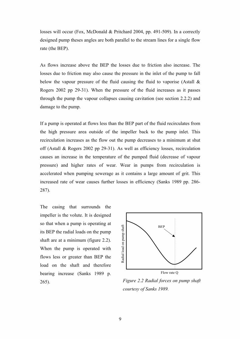
The casing that surrounds the
impeller is the volute. It is designed
so that when a pump is operating at
its BEP the radial loads on the pump
shaft are at a minimum (figure 2.2).
When the pump is operated with
flows less or greater than BEP the
load on the shaft and therefore
bearing increase (Sanks 1989 p.
265).
Flow rate Q
Rad
ial l
oad
on p
ump
shaf
t BEP
Figure 2.2 Radial forces on pump shaft
courtesy of Sanks 1989.
10
2.2.2 Cavitation
Cavitation occurs when bubbles of vapour form in a low pressure area and then
collapse as the fluid moves to a high pressure area inside the pump. The water
vapour bubbles form if the pressure in an area of a pump is lower than the vapour
pressure of the fluid. When the bubbles collapse the localized pressures that are
produced as the fluid moves in to the empty space are very large (Fox, McDonald
& Pritchard 2004, pp. 524-525).
Cavitation causes permanent pitting on the surfaces of the volute and impeller as
well as reducing pump performance. It occurs when pumps are operated at flow
rates either much greater or much less than their BEP (Sanks 1989 p. 255), in
areas of low pressures (pump inlet at high flows) or high local velocities (caused
by recirculation). The rough surface created by cavitation pitting creates further
flow disturbances and increases the amount of cavitation accelerating the
destruction of the pump (Astall & Rogers 2002 pp 29-33).
When cavitation occurs the bubbles collapsing sounds like pieces of gravel are
rolling around in the pump. The level of noise increases dramatically which is
undesirable in residential areas.

11
2.2.3 Recommended Operating Range
The range recommended by Tchobanoglous, (Sanks 1989 p. 255) for radial flow
centrifugal pump for continuous operation is between 60 and 120 percent of BEP
as shown in figure 2.3. Astall & Rogers on page 39 recommend between 50 and
110 percent of BEP as their recommended operating range.
Figure 2.3 Recommended operating range for centrifugal pumps
By operating within this range the effects of recirculation, cavitation and high
bearing loads will be avoided (Astall & Rogers 2002 p. 39). Operating for
extended periods outside this range will damage and shorten the useful life of the
pump (Sanks 1989 p. 255). Pump manufacturers will sometimes specify a
desirable range of operation on their pump performance curves.
Hea
d, E
ffic
ienc
y
BEP
0 50 100 120 %
Flow rate Q as a percentage of BEP
Recommended operating range

12
2.3 Pump Station Configuration Options
The pump station system resistance curves to be used for this investigation are
shown in figure 2.4 and have been provided by Citiwater. The Average Dry
Weather Flow (ADWF) has been also provided by Citiwater as 1.8 litres per
second.
Pump Station A11B System Curve
Revised Dry Weather Duty Point
Required Wet Weather Duty Point
0
5
10
15
20
25
30
0 10 20 30 40
Flow (l/s)
Hea
d (m
)
Minimum Dry WeatherFlow ConditionsAverage Dry WeatherFlow ConditionsWet Weather FlowConditions
Figure 2.4 System resistance curve for Pump Station A11B
Citiwater has specified the Required Wet Weather Duty (from section 2.1) as 5 x
ADWF or 9.0 litres per second at 21 m head. By taking into account the operation
requirements listed in section 2.3 the dry weather duty point has been revised to
4.8 x ADWF corresponding to 8.6 litres per second at 8.7 m head.
The pump station is located in a small laneway less than 2 m to residential
housing therefore pump speeds of greater than 1500 rpm may not be used
(Citiwater 2007, pers. comm., April 4).

13
2.3.1 Current Citiwater Method
The current method used by Citiwater is to install one small pump to operate
during normal dry weather and one large pump for wet weather conditions. The
small pump is to operate at the average dry weather flow conditions, the minimum
dry weather flow conditions and all points in between. The large pump must be
able to operate in the range between wet weather flow conditions and minimum
dry weather flow conditions. The large pump is used as the duty pump one week a
month during dry conditions to prevent the build up of solids inside the impeller
and to ensure it is in working order for the wet season (Citiwater 2007, pers.
comm., April 4).
Pump Station A11B System CurveExisting Method
0
5
10
15
20
25
30
0 10 20 30 40
Flow (l/s)
Hea
d (m
)
Minimum Dry WeatherFlow Conditions
Average Dry WeatherFlow Conditions
Wet Weather FlowConditions
Flygt NP3153.181impeller 454
Grundfos SV-034-DHU
BEP 35.3 l/s @ 15.9 mand 14.2 l/s @ 9.0 m
Figure 2.5 Pumps for Pump Station A11B selected using current method, pump
performance curves courtesy of Grundfos and Flygt.
Pump 1 ITT Flygt model NP3153.181 HT $ 17000.00
Pump 2 Grundfos SV-034-DHU $ 3400.00
$ 21400.00
For the pumps selected above the small pump will operate at approximately 12
litres per second for average conditions or at 85 % of BEP. During minimum flow
the pump would operate at 18 litres per second corresponding to 125 % of BEP.
14
This is outside the recommended range by a small amount 5 % but considering it
will only rarely operate in that condition it is considered acceptable.
When the large pump is used during dry weather it will operate between 25 and
35 litres per second, corresponding to 71 to 99 % of BEP which is inside the
recommended operating range. For wet weather flow conditions the pump will
operate at approximately 10 l/s which is 28 % of BEP. Accordingly it can be
expected that this pump will experience high radial loads and higher rates of wear
if operated during wet weather. As wet weather flow conditions occur less
frequently than dry these problems would not impact significantly the pumps
operation. A major disadvantage of this configuration is that the cost of the large
pump is five times the cost of the small pump, and its higher capacity that is only
required during wet weather.
Further if the large pump fails during wet weather the pump station wet well will
overflow as the capacity of the small pump is insufficient to cope with the wet
weather flows. This is not acceptable as it contradicts section 2.4 of the pump
station code, namely that the failure of any one piece of equipment should not
prevent the pump station from operating (WSA 2005 p.54).
15
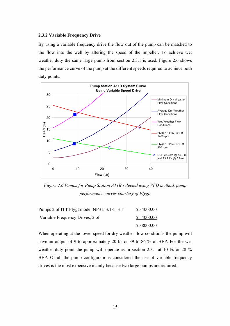
2.3.2 Variable Frequency Drive
By using a variable frequency drive the flow out of the pump can be matched to
the flow into the well by altering the speed of the impeller. To achieve wet
weather duty the same large pump from section 2.3.1 is used. Figure 2.6 shows
the performance curve of the pump at the different speeds required to achieve both
duty points.
Pump Station A11B System CurveUsing Variable Speed Drive
0
5
10
15
20
25
30
0 10 20 30 40
Flow (l/s)
Hea
d (m
)
Minimum Dry WeatherFlow Conditions
Average Dry WeatherFlow Conditions
Wet Weather FlowConditions
Flygt NP3153.181 at1460 rpm
Flygt NP3153.181 at 960 rpm
BEP 35.3 l/s @ 15.9 mand 23.2 l/s @ 6.9 m
Figure 2.6 Pumps for Pump Station A11B selected using VFD method, pump
performance curves courtesy of Flygt.
Pumps 2 of ITT Flygt model NP3153.181 HT $ 34000.00
Variable Frequency Drives, 2 of $ 4000.00
$ 38000.00
When operating at the lower speed for dry weather flow conditions the pump will
have an output of 9 to approximately 20 l/s or 39 to 86 % of BEP. For the wet
weather duty point the pump will operate as in section 2.3.1 at 10 l/s or 28 %
BEP. Of all the pump configurations considered the use of variable frequency
drives is the most expensive mainly because two large pumps are required.

16
2.3.3 Parallel Operation
If two identical pumps are operated in parallel as shown in figure 2.7 the resulting
performance curve is found by added the flow capacities at each head (Fox,
McDonald & Pritchard 2004, p. 537).
Figure 2.7 Schematic representation of pumps operating in parallel
The same system curve is shown in figure 2.8 for two smaller pumps operating in
parallel. To satisfy the redundancy requirements of section 2.4 of the pump station
code three pumps would need to be installed. During normal operation there
would be one duty and two standby and for wet weather two duty pumps with one
standby.
Pump Station A11B System CurveSingle Speed Pumps in Parallel
0
5
10
15
20
25
30
0 10 20 30 40
Flow (l/s)
Hea
d (m
)
Minimum Dry WeatherFlow Conditions
Average Dry WeatherFlow Conditions
Wet Weather FlowConditions
Two SV-042-DS50 inparallel
SV-042-DS50
BEP 9.69 l/s @ 13.6 m and 19.4 l/s @ 13.6 m
Figure 2.8 Pump Station A11B with pumps in parallel.
Pumps 3 of Grundfos SV-042-DS50 $ 10800.00
Swing check valves
17
For normal flow conditions the single pump will operate between 12 and 16 litres
per second which corresponds to 123 to 155 % of BEP, which is above the
recommended maximum. For wet weather flows the two pumps will operate at 9
litres per second or 46 % of BEP, which is below the recommended minimum.
These pumps also operate at 2900 rpm. All of the above factors make these pumps
unsuitable for this application.
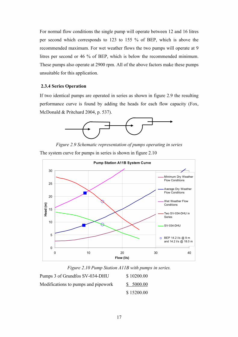
2.3.4 Series Operation
If two identical pumps are operated in series as shown in figure 2.9 the resulting
performance curve is found by adding the heads for each flow capacity (Fox,
McDonald & Pritchard 2004, p. 537).
Figure 2.9 Schematic representation of pumps operating in series
The system curve for pumps in series is shown in figure 2.10
Pump Station A11B System Curve
0
5
10
15
20
25
30
0 10 20 30 40Flow (l/s)
Hea
d (m
)
Minimum Dry WeatherFlow Conditions
Average Dry WeatherFlow Conditions
Wet Weather FlowConditions
Two SV-034-DHU inSeries
SV-034-DHU
BEP 14.2 l/s @ 9 m and 14.2 l/s @ 18.0 m
Figure 2.10 Pump Station A11B with pumps in series.
Pumps 3 of Grundfos SV-034-DHU $ 10200.00
Modifications to pumps and pipework $ 5000.00
$ 15200.00

18
For normal flow conditions the single pump will operate between 12 and 18 litres
per second which is 85 to 125 % of BEP. For wet weather flows the two pumps
will operate at 10 litres per second or 70 % of BEP. The pumps operate at 1450
rpm. All these factors are acceptable.
The current method for pumps to operate in series requires then to be permanently
connected as shown in figure 2.9. Therefore two pumps would have to be
connected in series and a third pump installed to operate by itself for normal
operation. This arrangement is not acceptable as the failure of any one of the three
pumps would prevent the pump station from operating properly.
If pumps could operate as a stand alone pump for normal operation but have
piping and valving that connected them in series for wet weather operation this
problem would be overcome. A possible arrangement is shown in figure 2.11.
Figure 2.11 Pipe configuration that will allow pumps to operate in series or
singularly.
Normal operation requires either pump to run. If pump 1 is running pressure
produced by the pump closes check valve 2a forcing the fluid into the pressure
main. If pump 2 is operating fluid is drawn in through check valve 2a through the
pump and into pressure main (P3). Check valve 1 closes preventing recirculation.
When a single pump is operating there will be some flow through the pump that is
not running.
For wet weather operation both pumps need to operate. Pressure at P3 is greater
than the pressure Pump 1 can produce therefore check valve 1 is forced closed. P2
is greater than P1 forcing 2a closed and the fluid into Pump 2. This allows the
Pressure main
Swing check valves
Swing check valve
Pump 1
Pump 2 2b
1
2a
Connection Line P3 P1 P2
19
pumps to operate in series resulting in the performance curve shown in figure
2.10.
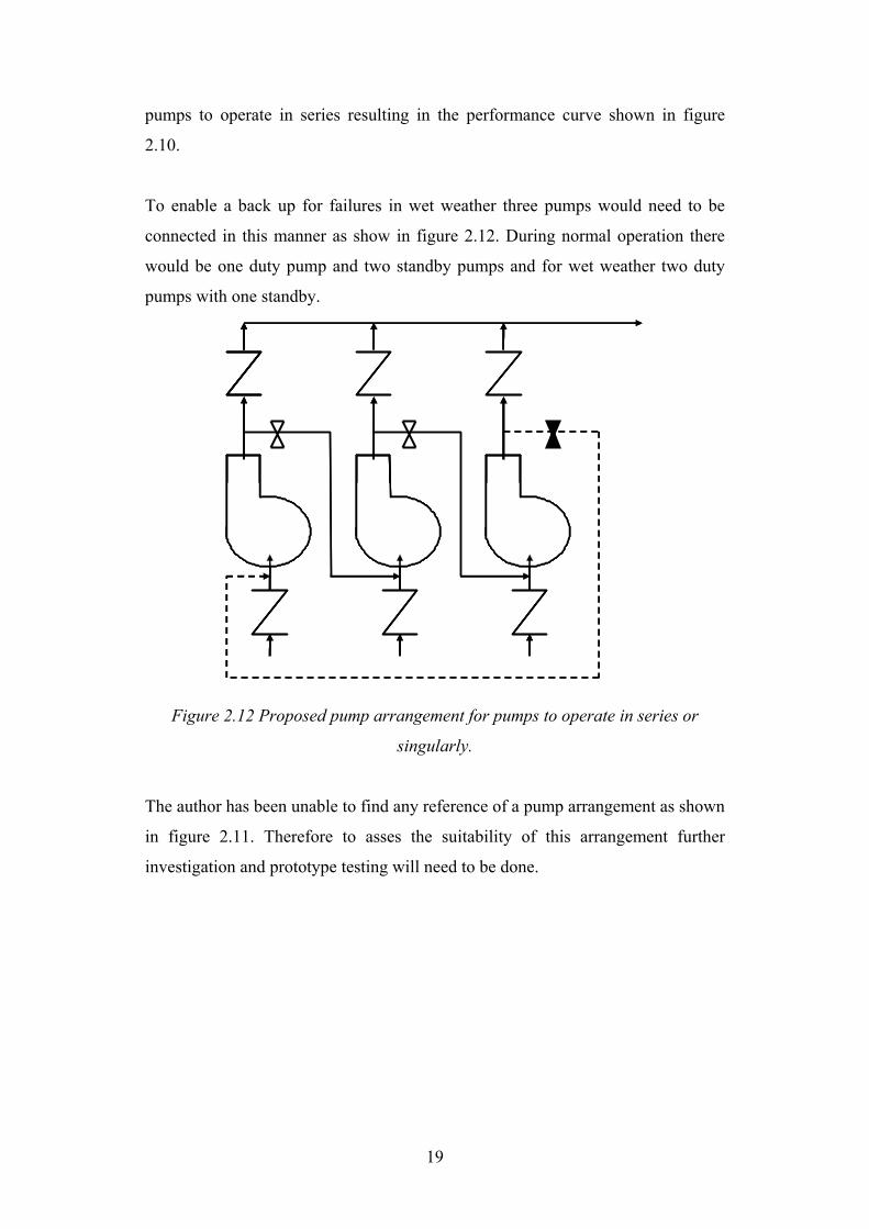
To enable a back up for failures in wet weather three pumps would need to be
connected in this manner as show in figure 2.12. During normal operation there
would be one duty pump and two standby pumps and for wet weather two duty
pumps with one standby.
Figure 2.12 Proposed pump arrangement for pumps to operate in series or
singularly.
The author has been unable to find any reference of a pump arrangement as shown
in figure 2.11. Therefore to asses the suitability of this arrangement further
investigation and prototype testing will need to be done.

20
2.3.5 Summary
Table 2.1 lists all the above configurations and allocates a quantitative score to
predicted operating performance. The score ranges from 5 as satisfying all
requirements to 0 as not being suitable at all. A total of the quantitative scores for
each configuration are given at the bottom of table 2.1.
Pump Configuration Current Method Variable Speed Parallel operation Series operation
Dry weather operating range
(% of BEP) 85 - 125 39 - 86 123 -155 85 - 125
Suitability Score 4 4 0 4
Wet weather operating point
(% of BEP) 28 28 46 70
Suitability Score 3 3 4 5
Backup Provision for Pump
Failure
None if large
pump fails in wet
weather
One duty one
standby in wet
and dry weather
One duty two standby in dry
weather, two duty and one standby
in wet weather
Suitability Score 0 5 5 5
Cost $21,400.00 $ 38,000.00 $10,800.00 $15,200.00
Comparative Score 2.5 1.4 5.0 3.6
Total 9.5 13.4 14.0 17.6
Table 2.1 Comparison of pump configuration options
2.4 Conclusions: Chapter 2
Of the alternatives to the current Citiwater design all three pump station
configurations satisfy the requirements of the pump station code. Only the
variable frequency drive method and the proposed series operation allow the
pumps to operate within the recommended operating range.
The use of variable frequency drives is recognised as an acceptable solution for
large pump stations or to maintain continuous flow into a treatment plant. The
major problem of variable frequency drives is the extra cost of the drive and the
need to install larger pumps. For normal dry weather operation less than half of
the pumps flow capacity is utilised. For the small and medium sized stations
21
which make up 98 of the 102 pump stations at Citiwater, this extra cost is
significant.
The suitability of the series configuration in a sewerage system is unknown
without further investigation. This project will design and build a prototype of this
series configuration and assess its performance.

22
Chapter 3: Prototype Design To assess the suitability of the series pump configuration a working prototype was
designed. The prototype design aims to incorporate all the operational functions of
the proposed series configuration referred to in figure 2.12. The eventual plan was
to test the prototype in the actual sewerage system therefore the design would
have to comply with the requirements discussed in section 2.1
3.1 Design Process
Y
Are pumps operating between 50-120% of
BEP for both duty points?
Build prototype
Y
Y
Design Prototype
Does design satisfy Section 2.1 pump
station requirements?
Does mathematical model of prototype
achieve duty points?
N
Figure 3.1 Design process flow diagram.
23
3.2 Design Considerations
The recommendations from both WASA and Citiwater state small to medium
pump station should be of a wet well design to as discussed in section 2.1. This
requires the pumps to be able to be removed from wet well for maintenance. The
major difference between the proposed series pump configuration and existing
designs was the need for two pipes to be connected to the pump instead of one.
This was achieved by modifying the manufacturer’s current auto couple design
which is explained in detail in section 3.2.1.
Some other design considerations that were included in prototype design included
• When operated in series the pressure produced by second pump should be
less than the pressure rating of the pump.
• Where possible “off the shelf” components such as valves, swing check
valves, pump auto couples and pipe fittings were used.
• The pipework between the two pumps (the series connection) must be a
design that does not allow air to build up and become trapped. Entrapped
air can reduce the flow through the pipe and may cause loss of prime in
pump (Astall & Rogers 2002 Sec. 2 p 5)
• The volutes of both pumps must be fully submersed at well start height to
ensure they were always fully primed when they needed to run.
• The two pumps can not be connected together rigidly as vibrations
produced when only one pump is running may cause the bearings in the
stopped pump to brinnel.
3.3 Component Design
Two components were identified as not being readily available products and
therefore had to be designed;
1. The under pump valve which is a non return (swing check) valve that has
two inlets to allow automatic switching between single pump operation
and series pump operation.
2. An auto couple that would allow connections to the inlet and outlet of a
submersible pump and;

24
3.3.1 Under pump valve
The non return valve that is fitted to the inlet side of the pump was modified to
incorporate a second inlet making it a three way valve. This modification was
done to make the valve more compact and to decrease flows through the pump
that was not operating.
Making the under pump valve and pipework more compact meant that the pump
could be positioned closer to the bottom of the well. This allows the volute of the
pump to be fully submerged at lower well levels. Figure 3.2 shows a reduction in
length of 290 mm was achieved by moving the inlet to be part of the valve.
620
330
(a)(b) (c)
Figure 3.2 Under pump valve a) if not modified, b) modified single pump
operation and c) modified series pump operation.
When the pump is operating as a single pump some of the inlet flow will be drawn
in through the adjacent pump as explained in section 2.3.4. Figure 3.2 (b) shows
that the pipe that is connected to the adjacent pump is shut off when the pump is
operating as a single pump. It is hoped that this will reduce flows through the non
operating pump and reduce the risk of blockage.
3.3.2 Auto Couple Design
A sewerage wet well is a confined space with a high probability of hydrogen
sulphide gas being present. The risk assessment (Appendix B) identified entry into
the wet well for routine maintenance of pumps as an unacceptable risk. Current
submersible pump designs utilise an auto coupling device that takes advantage of
the pumps weight to form the seal between the pump outlet and sewerage system
piping, (refer to figure 3.3). A pedestal remains in the well and is permanently

25
attached to the pressure main. It has guide rails to ensure pump is located
correctly when lowered down into the well.
Figure 3.3 Submersible pump being lowered onto pedestal.
To allow the modified pump to be removed from the wet for maintenance a
system to connect the pump to two pipes had to be developed. The extra swing
check valve that was to be connected to the inlet of the pump was identified as a
possible blockage point and was therefore connected to the bottom of the pump.
This would allow the valve to be removed and inspected by simply lifting the
pump out of the well.
An extra auto couple was purchased and the pump pedestal modified to enable the
two auto couples to be arranged side by side as shown in figure 3.4. Detailed
information on the load carrying capacity and the force required for the auto
couple to seal was not available. The loads on an unmodified pump were
calculated and used to dimension the new auto couple design. Factors taken into
consideration included the use of two auto couples to share the load, providing
space for the extra pipework and higher pressures produced by the pump when
operating in series. Details of these calculations may be found in appendix D.

26
Rubber pipe expansion joint to prevent transmission of vibration through pipe.
Under pump non return valve modified with two inlets to lower pump and reduce blockages
Modified auto couple which allows the connection of two pipes into single pump
No high spots in pipe work which would allow air to accumulate
Modified pump pedestal
Distance between pump and pedestal increased to ensure auto couple would seal at the higher pressures when pumping in series
Resilient seated gate valve which will be shut only when one of the pumps is removed from the well
Figure 3.4 Final prototype design showing key design features.
Figure 3.4 illustrates the solutions the author used to meet the design requirements
listed in section 3.2. Full detail arrangement and construction drawings are shown
in appendix C. All design drawings were done by the Citiwater draftsperson
Kevin McGrath under the direction of the author.

27
3.3.3 Pump Casing Pressure Rating
From the manufacturer’s specification the maximum head produced by a singular pump is 14 m. For water at 25°C the corresponding discharge pressure (P1) is
1P ghρ∴ = (3.1)
997 9.81 14137 kPa gauge
= × ×=
The maximum discharge pressure able to be developed by two pumps in series is
12 274 kPaP = . (3.2)
Also from the manufacturer’s specifications (refer appendix E) the rating of the
pump casing is PN 10, which corresponds to a nominal working pressure of 1000
kPa (AS/NZS 4129-2000). Therefore the maximum pressure able to be produced
by the two pumps operating in series is within the pressure rating of the pump.
3.3.4 Materials
Where applicable the guide lines from WSA 101-2005 were used for material
choice. Table 3.1 summarises materials used in major components.
Component Material Notes
Pumps and
pedestal
Grey Cast Iron with
manufacturer’s coating
WSA 101-2005 page 8
Guide rail and pipe 316 stainless steel WSA 101-2005 page 8
Valves Ductile Iron with
nylon coating
See appendix E
Valve discs EPDM with ductile
iron core
Expansion joint Nitrile Hydrocarbons often present in
raw sewerage
Table 3.1 Material use summary.
Full details of materials used in purchased components may be found in appendix
E, which contains the manufacturer’s specifications.

28
3.4 Model Calculations
To check if the above design would operate with acceptable performance before it
was constructed a mathematical model was created. To calculate the overall
performance of the series pump configuration, flow head data from the pump
manufacturer’s performance curve was used. The head loss due to friction was
subtracted from various flows, to obtain an estimate of the performance curves
after the pumps have been modified. The friction losses taken into account are
caused by the length of pipe and the extra pipe fittings needed to connect the two
pumps. They are estimated by the following equations;
Pipe friction loss: 2
2lLVH fd g
= (3.3)
Fitting friction loss: 2
2lVH k
g= (3.4)
where Hl is head loss [m]
f is the friction factor obtained from the Moody diagram
L is the length of pipe [m]
V is the velocity of sewage through the pipe [m/s]
d is the diameter of the pipe [m]
g is the acceleration due to gravity [m/s2]
k is the resistance coefficient of the valves and fitting obtained
from Chart 14 of AS-2200:2006.
The values for the flow head curve were then plotted over the system curve for the
pump station to be used in this trial. A plot of pumps connected in a conventional
series configuration as shown in figure 2.9 is also included for comparison. The
plot is shown in figure 3.5. Detail of the calculations and values used may be
found in appendix F.

29
Head Loss due to Modifications
0
5
10
15
20
25
30
0 10 20 30Flow (l/s)
Hea
d (m
)Pumps connected inseries with no frictionlossPumps 1 and 2Connected in Series
Single UnmodifiedPump
Single Modified Pump
Wet Weather FlowConditions
Average Dry WeatherFlow Conditions
Minimum Dry WeatherFlow Conditions
Duty Points
Figure 3.5 Performance estimates after pumps have been modified
Figure 3.5 shows that when the two pumps are operating under wet weather
conditions there will be a loss in flow of approximately 0.5 l/s compared to the
ideal model that ignores friction in the connecting pipes and fittings. It is also
shown that for average flow conditions the loss in flow from the pump is
negligible and for minimum flow there is a flow loss of less than 0.5 l/s. The
model shows resulting flows will still exceed both required duty points and would
be acceptable for construction of prototype.

30
Chapter 4: Prototype Testing The prototype pumps were installed in a testing tank to check the system
components operated as intended and to confirm the mathematical model from
section 3.4. The tests were also used to measure the flows through the non
operating pump when the pumps were operating as a single pump.
Figure 4.1 Prototype pumps installed in test tank.

31
4.1 Flow and Pressure measurement
The flow rate in the test circuit was controlled with a butterfly valve (shown as
control valve). The flow rate of each pump was measured by two magnetic flow
metres installed as shown in figure 4.2.
Figure 4.2 Schematic of test tank showing location of flow metres and pressure
tappings
The pumps were installed in the test tank and pressure measurement lines were
attached to the prototype at the locations shown in figure 4.2. The black flexible
tubes that can be seen in figure 4.1 are the pressure lines. The pressure tapping
shown above as P1 was level with the inlets of both pumps. It was connected to
one side of a differential pressure gauge to provide a reference pressure as
illustrated in figure 4.3.
Pressure lines p2 to p6 were attached to a manifold that was connected to the other
side of the differential pressure gauge. Before measurements were taken all the air
in the pressure lines was bled out.
Flow
meter 2
Flow
meter 1
p1
p2
p3 p4
p5
p6
Control
valve

32
Figure 4.3 Arrangement of pressure gauge which enabled all pressures to be
measured with one instrument
This arrangement allowed the pressure difference to be recorded with one
instrument. Also, there was no need to take into account the difference in height
between the gauge location and the pressure tapping points.
The value displayed on the pressure gauge is ∆px-1 with x determined by which
valve is open on the manifold. As the water in the test tank is recirculated, after a
short period of time the level in the tank will achieve steady state and p1 will be
constant. Therefore the pressure difference between any two measurement points
in the prototype may be calculated with equation 4.1.
1 1a b a bp p p− − −∆ = ∆ − ∆ (4.1)
p2 p3 p4 p5 p6 p1
Pressure line manifold
Differential
pressure gauge

33
Figure 4.4Differential pressure gauge and manifold connected to the side of the
test tank.
4.2 Test Tank Results
The purpose of the first series of tests was to determine the validity of the
mathematical model from section 3.4. The model is a prediction of the final head
flow performance curve. The values used in the model were flow in litres per
second and pump head (HP) which is the energy per unit of weight of flowing
fluid, (Fox, McDonald & Pritchard 2004, pp. 336) and measured in metres. The
flow rate through each pump can be obtained directly from the flow metres but HP
must be calculated from a combination of pressure and flow rate measurements.
HP is described by Fox et al. on page 501 with equation (4.2)
2 2
discharge suction2 2Pp V p VH z zg g g gρ ρ
⎛ ⎞ ⎛ ⎞= + + − + +⎜ ⎟ ⎜ ⎟⎝ ⎠ ⎝ ⎠
(4.2)
Where p is absolute pressure, ρ density of the fluid, g is gravitational acceleration
(9.81 m.s-2), V is the velocity of the fluid and z is the relative height in metres.
The pressure at the suction is measured with pressure tapping p1 where
0 m/sV ≈ . discharge suctionz z= as both pressures are measured with the same
instrument, see section 4.1 above. So equation 4.2 reduces to

34
2discharge suction discharge 1
2P
p p VH
gρ
⎛ ⎞−= +⎜ ⎟⎜ ⎟⎝ ⎠
(4.3)
V may be obtained by equation 4.4
discharge 2
4Q QVA Dπ
= = (4.4)
Where D is the discharge internal diameter in metres and Q is the flow rate of the
fluid in m3/s. The diameter of each pump discharge is 80 mm.
4.2.1 Pump 1 Performance
The first pump tested was pump No. 1 which is the unmodified pump. Its
measured performance in the test tank was compared to the manufacturer’s data
from appendix E. Table 4.1 shows the test and calculated data.
Pump 1 Test Results (unmodified pump) Test data Calculated data
Q (l/s) p2-1 (kPa) V (m/s) HP (m) 29.7 8 5.91 2.60 27.3 18 5.43 3.34 24.8 30 4.93 4.31 22.2 43 4.42 5.39 20 54 3.98 6.33
18.1 63 3.60 7.10 15.8 79 3.14 8.58 13.6 92 2.71 9.78 11.1 106 2.21 11.09 9.6 112 1.91 11.64 7.1 121 1.41 12.47 4.2 128 0.84 13.12 2.2 132 0.44 13.51 0 135 0.00 13.80
Table 4.1 Test results for Pump 1
Figure 4.5 shows this data on a pump head flow curve compared to the
performance data supplied by the pump manufacturer. It shows test results and the
performance claimed by the manufacturer are very similar. The test results
showed a small increase in head produced at flow rates above 20 l/s. This
difference may be due to small variations in pump performance of the same model
pump where as the performance data published by the manufacturer is the
average.
35
Pump 1 Performance
0
2
4
6
8
10
12
14
16
18
20
0 10 20 30
Flow (l/s)
Pum
p H
ead
(m)
Manufacturer's data
Test results
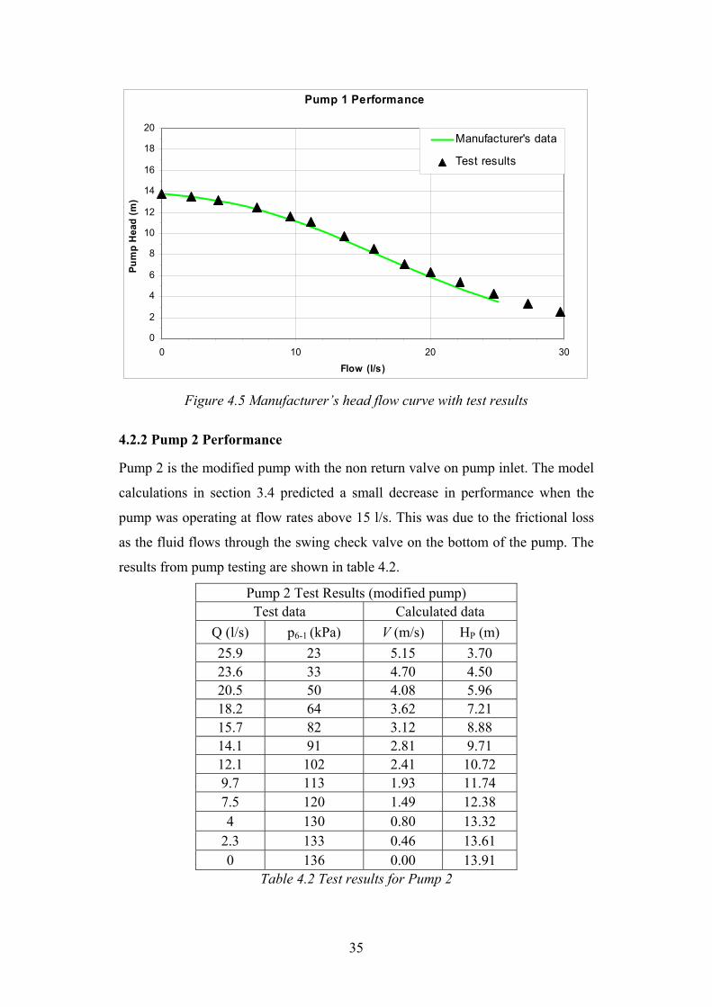
Figure 4.5 Manufacturer’s head flow curve with test results
4.2.2 Pump 2 Performance
Pump 2 is the modified pump with the non return valve on pump inlet. The model
calculations in section 3.4 predicted a small decrease in performance when the
pump was operating at flow rates above 15 l/s. This was due to the frictional loss
as the fluid flows through the swing check valve on the bottom of the pump. The
results from pump testing are shown in table 4.2.
Pump 2 Test Results (modified pump) Test data Calculated data
Q (l/s) p6-1 (kPa) V (m/s) HP (m) 25.9 23 5.15 3.70 23.6 33 4.70 4.50 20.5 50 4.08 5.96 18.2 64 3.62 7.21 15.7 82 3.12 8.88 14.1 91 2.81 9.71 12.1 102 2.41 10.72 9.7 113 1.93 11.74 7.5 120 1.49 12.38 4 130 0.80 13.32
2.3 133 0.46 13.61 0 136 0.00 13.91
Table 4.2 Test results for Pump 2
36
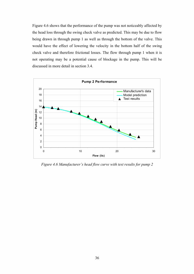
Figure 4.6 shows that the performance of the pump was not noticeably affected by
the head loss through the swing check valve as predicted. This may be due to flow
being drawn in through pump 1 as well as through the bottom of the valve. This
would have the effect of lowering the velocity in the bottom half of the swing
check valve and therefore frictional losses. The flow through pump 1 when it is
not operating may be a potential cause of blockage in the pump. This will be
discussed in more detail in section 3.4.
Pump 2 Performance
0
2
4
6
8
10
12
14
16
18
20
0 10 20 30
Flow (l/s)
Pum
p H
ead
(m)
Manufacturer's dataModel predictionTest results
Figure 4.6 Manufacturer’s head flow curve with test results for pump 2

37
4.2.3 Both Pumps Operating Performance
With both pumps running at the same time and with the control valve fully open
to simulate low system resistance, it was observed that significant flows were
recorded flowing out the pipe above pump 1. This indicates the check valves
above pump 1 and below pump 2 were not fully closed and the pumps were
operating in parallel. Table 4.3 shows that this only happens at head pressures of
less than 5 metres which is below the minimum system curve and therefore would
not occur when the pumps are operating in pump station.
Pumps 1 & 2 Both Running Test Results Test data Calculated data
Q1 (l/s) Q2 (l/s) Q Total (l/s) p6-1 (kPa) V (m/s) HP (m) 17.7 26.8 44.5 17 5.33 3.19 14 27 41 20 5.37 3.52
12.6 26.2 38.8 22 5.21 3.63 11.3 25.6 36.9 26 5.09 3.98 7.6 24.6 32.2 30 4.89 4.29 5.1 24.8 29.9 33 4.93 4.61 2.3 23.4 25.7 36 4.66 4.79 0.5 22.9 23.4 38 4.56 4.94 0 21.8 21.8 66 4.34 7.71 0 18.4 18.4 110 3.66 11.93 0 15.7 15.7 150 3.12 15.83 0 13.3 13.3 179 2.65 18.66 0 11.5 11.5 202 2.29 20.92 0 9 9 224 1.79 23.07 0 6.1 6.1 246 1.21 25.23 0 2.7 2.7 262 0.54 26.80 0 0 0 272 0.00 27.81
Table 4.3 Test results for Pumps 1 and 2 operating at the same time
Figure 4.7 illustrates the predicted performance curve closely matches the actual
test performance. The transition between series and parallel operation discussed
above can be observed by the sharp turn in the performance curve at the flow rate
of 24 l/s.

38
Both Pump Operating Performance
0
5
10
15
20
25
30
0 10 20 30 40 50
Flow (l/s)
Pum
p H
ead
(m)
Manufacturer's data
Pump in series (no losses)
Model prediction
Test results
Figure 4.7 Head flow curve for Pump 1 + Pump 2
The performance of the pumps in both operating modes (single pump and in
series) are generally consistent with and slightly exceed the mathematical models
from section 3.4. They are therefore appropriate to install in sewerage system.
4.3 Flows through Standby Pump
As mentioned above when a single pump was operating alone there is a
significant flow through the non operating pump. This may allow solids to
accumulate in the volute of the pump and increase the risk of blockage.
When pump 1 was operating the flow through the non operating pump could be
measured with the flow metre above pump 2. It can be seen from table 4.4 that the
flows of up to 25 % of the total flow were observed going through pump 2 while
it was not running.
Q1 (l/s) Q2 (l/s) Q Total (l/s) Flow though standby pump
16.4 2.7 19.1 14% 10.1 2.5 12.6 20% 8.6 2.8 11.4 25% 6 0.8 6.8 12% 3 0.1 3.1 3%
Table 4.4 Flow rate thorough non operating pump 2 with pump 1 running

39
To estimate the flows through pump 1 when pump 2 was running equation 4.5
was used 2 2 2
2 42 2 2p V p V Vz z Kρ ρ
⎛ ⎞ ⎛ ⎞ ⎛ ⎞+ + − + + =⎜ ⎟ ⎜ ⎟ ⎜ ⎟
⎝ ⎠ ⎝ ⎠ ⎝ ⎠ (4.5)
where K is the loss coefficient of the pipe fittings between pressure tapping points
2 and 4 (see figure 4.2) . As the pipe diameter at point 2 and 4 are equal 2 4V V= ,
the pressures are measured on the same elevation 2 4z z= and 31000 kg/mρ ≈
equation 4.5 reduces to 2
2 4 kPa2
Vp p K⎛ ⎞
− = ⎜ ⎟⎝ ⎠
(4.6)
where pressure is measured in kPa.
The loss coefficient K was obtained from test data when both pumps were running
and all flow was going through the connecting pipe. These results are summarised
in table 4.5.
Q1 (l/s) Q2 (l/s) Q Total (l/s) ∆p2-4 (kPa) V4 (m/s) K 0 23 23 20 4.6 1.9 0 21.1 21.1 16 4.2 1.8 0 13.1 13.1 6 2.6 1.8 0 9.3 9.3 4 1.9 2.3 0 4.4 4.4 1 0.9 2.6 0 2.1 2.1 0.5 0.4 5.7
Table 4.5 Loss coefficient for connecting pipework
A value of K = 1.9 was chosen as the best fit of the above data and this is shown
graphically in figure 4.8.

40
Loss Coefficient Estimation
0
2
4
6
8
10
12
14
16
18
20
0.0 1.0 2.0 3.0 4.0 5.0
Velocity (m /s)
Pres
sure
dro
p (k
Pa)
Experimental data
K = 1.9
Figure 4.8 Loss coefficient K2-4 estimation
Therefore from above the flow through pump one when only pump 2 is operating
may be estimated with equation 4.7.
Q VA=
( ) 2
2 4Pump 1
2 kPa1.9 4
p p dQ π−= × m3/s (4.7)
Results from test data and equation 4.7 are summarised in table 4.6 and show
flows of approximately 25 % of the total flow pass through the standby pump
Q2 (l/s) ∆p2-4 (kPa) Qpump 1 (l/s) Flow though standby pump 26.3 1.5 6.3 24% 19.3 0.8 4.6 24% 14.9 0.5 3.6 24% 8.3 0.2 2.3 28% 2.4 0 0.0 0%
Table 4.6 Flows thorough pump 1 when not operating
Tests showed that up to 25 % of the pump stations output will pass through a
stationary pump when only one pump is operating. To prevent solids build up it is
recommended the pumps should operate with alternating duty which is discussed
in more detail in section 5.1.

41
Chapter 5: Operation in Pump Station
5.1 Pump Control Method
The switching between single pump operation and two pumps operating in series
must be simple and self controlling. This is achieved by the starting and stopping
of the pumps based on level in the wet well. This eliminates the need for control
valves or actuators to be located in the corrosive environment of the wet well. All
controlling of the pumps is done by a PCL controller located in the switchboard.
There were only minor changes to the logic currently used by Citiwater in other
pump stations. This approach was followed to decrease unforseen problems that
may occur with completely new logic.
Figure 5.1 Schematic of pump start and stop levels
The operation of the pumps is dictated by well level which is measured by a
hydrostatic pressure sensor. For normal dry weather operation only one pump is
required to achieve the necessary flow rate. When the well level fills to “start duty
pump” as shown in figure 5.1 the duty pump will start. When the well is drawn
Start standby pump
Start duty pump
Stop all pumps
Point for sewer main
pressure measurements

42
down to “stop all pumps” level the duty pump is stopped. To prevent solids
accumulating in the pump that is not operating the duties will alternate between
each pump.
If the well level rises to “start first pump” causing the duty pump to start and then
the level continues to rise the flow into the well is greater than the output of a
single pump. The most common reason for this is that the flow out of the pump
has been reduced due to an increase in pressure in the receiving main caused by
other pump stations in the sewerage system activating. When the level rises to
“start standby pump” the second pump will start causing the pumps to operate in
series. Both pumps will continue to operate until the well level has been lowered
to the “stop all pumps” level. The start stop levels used when the pumps were
installed is summarised in table 5.1.
Control function Level (m)
Stop all pumps 0.6
Start duty pump 1.2
Start standby pump 2.0
Table 5.1 Initial control level for pumps
43
5.2 Dry Weather Operation
The prototype pumps were installed in sewerage pump station A11B during July
2007 and commenced operating on the 22nd July 2007. There was no significant
rain in Townsville during the time period that this data presented below was
collected, therefore all operation was been under dry weather flow conditions. The
main operating criterion from section 2.2.3 was that the pumps operated between
50 and 120 percent of their best efficiency point in regard to flow. The best
efficiency flow rate for the pumps used in the prototype is 14.2 l/s (see section
2.3.4 figure 2.10), consequently the pumps should operate between 7.1 and 17.0
litres per second.
Pump Station Flow Rates for Dry Weather (Single Day)
6.0
7.0
8.0
9.0
10.0
11.0
12.0
13.0
14.0
15.0
0:00:00 3:00:00 6:00:00 9:00:00 12:00:00 15:00:00 18:00:00 21:00:00 0:00:00Tim e of Day
Flow
(l/s
)
Flow Rate Pump 1 (average 11.6 l/s)Flow Rate Pump 2 (average 11.9 l/s)
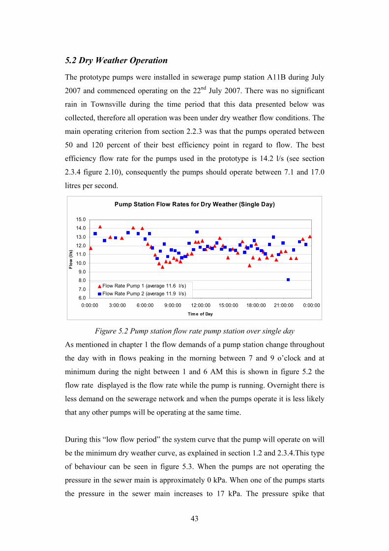
Figure 5.2 Pump station flow rate pump station over single day
As mentioned in chapter 1 the flow demands of a pump station change throughout
the day with in flows peaking in the morning between 7 and 9 o’clock and at
minimum during the night between 1 and 6 AM this is shown in figure 5.2 the
flow rate displayed is the flow rate while the pump is running. Overnight there is
less demand on the sewerage network and when the pumps operate it is less likely
that any other pumps will be operating at the same time.
During this “low flow period” the system curve that the pump will operate on will
be the minimum dry weather curve, as explained in section 1.2 and 2.3.4.This type
of behaviour can be seen in figure 5.3. When the pumps are not operating the
pressure in the sewer main is approximately 0 kPa. When one of the pumps starts
the pressure in the sewer main increases to 17 kPa. The pressure spike that

44
occurred just after 1:15 AM is a result another pump running elsewhere in the
sewerage network. The flow from each pump is at a maximum when the pump
starts as the well has reached the start duty pump level. The flow steadily reduces
to a minimum at the pump stop level as the fluid has to be lifted higher as the
level in the well lowers.
Pump Output Dry WeatherLow Flow Period
02468
1012141618202224
1:00:00 AM 1:15:00 AM 1:30:00 AM 1:45:00 AM 2:00:00 AMTim e of Day
Flow
(l/s
)
-120-100-80-60-40-20020406080100120
Gau
ge P
ress
ure
(kP
a)
Pump 1
Pump 2
Sewer Pressure(Av = 15 kPa)
Figure 5.3 Pump station outflow and pressure during low flow period
This low flow period is when the pumps will have the highest possible flow rate.
The maximum flow shown is approximately 15 l/s. As this occurs when no other
pumps are operating it is unlikely that a higher flow will occur without changes to
the sewerage pipe network or the start level in the well is increased. As this is
inside the recommended operating range of 8.5 to 17 l/s this is acceptable. From
figure 4.5 and 4.6 there is approximately 1.5 metres of pump head difference
between 15 and 17 l/s. Therefore the start duty pump level (figure 5.1) could be
raised up to 1.5 metres without causing the pumps to operate outside the
recommended operating maximum of 17 l/s.
The minimum flow rate is expected when the inflow into the sewerage network is
at a maximum. During this period there is a higher probability that some of the
other pump stations in the sewerage network will be operating at the same time
with the effect of increasing the pressure at pump station A11B.
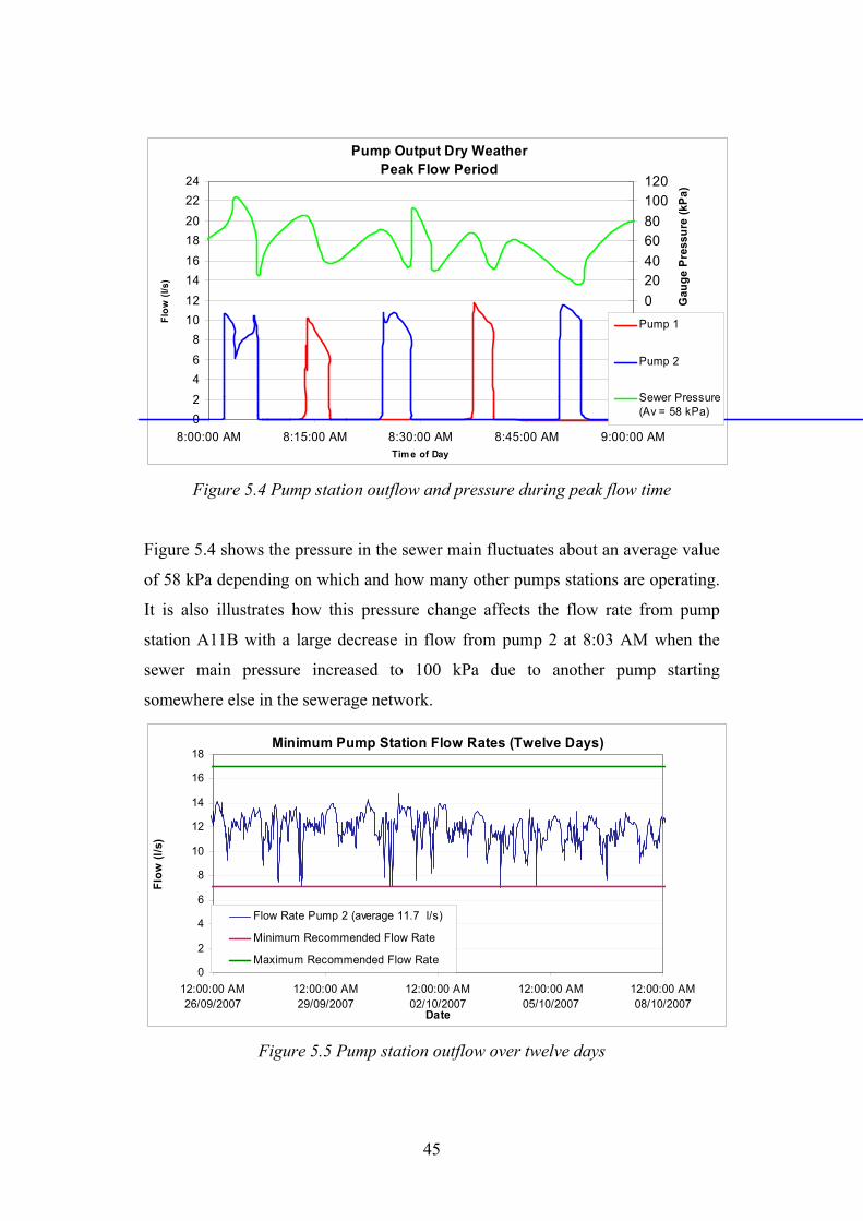
45
Pump Output Dry WeatherPeak Flow Period
02468
1012141618202224
8:00:00 AM 8:15:00 AM 8:30:00 AM 8:45:00 AM 9:00:00 AMTim e of Day
Flow
(l/s
)
-120-100-80-60-40-20020406080100120
Gau
ge P
ress
ure
(kPa
)
Pump 1
Pump 2
Sewer Pressure(Av = 58 kPa)
Figure 5.4 Pump station outflow and pressure during peak flow time
Figure 5.4 shows the pressure in the sewer main fluctuates about an average value
of 58 kPa depending on which and how many other pumps stations are operating.
It is also illustrates how this pressure change affects the flow rate from pump
station A11B with a large decrease in flow from pump 2 at 8:03 AM when the
sewer main pressure increased to 100 kPa due to another pump starting
somewhere else in the sewerage network.
Minimum Pump Station Flow Rates (Twelve Days)
0
2
4
6
8
10
12
14
16
18
12:00:00 AM26/09/2007
12:00:00 AM29/09/2007
12:00:00 AM02/10/2007
12:00:00 AM05/10/2007
12:00:00 AM08/10/2007
Date
Flow
(l/s
)
Flow Rate Pump 2 (average 11.7 l/s)
Minimum Recommended Flow Rate
Maximum Recommended Flow Rate
Figure 5.5 Pump station outflow over twelve days

46
Figure 5.5 shows the flow rates achieved by Pump 2 over a twelve day period.
The flow shown is the last flow recorded before the pump was stopped. Also
shown is the flow range recommended by Sanks, Astall & Rogers (refer section
2.2) It can be seen for most of the time the Pump 2 is operating within this range
except for the odd occasion when it operated at the minimum recommended flow
rate. The average flow rate achieved over this period was 11.7 l/s which exceeded
the minimum required by Citiwater of 8.6 l/s (section 2.3).
5.3 Simulated Wet Weather Operation
In the time between the installation of the pumps in the pump station and the
writing of this dissertation there has been no significant rain event in Townsville.
Consequently the testing of the prototype pumps under these “real life” wet
weather conditions has not been possible. Due to major road works in a nearby
sewerage network an opportunity became available to simulate the higher inflow
rates that occur under wet wether flow conditions. A section of the nearby
network had to be relocated, while this work was done and all flow had to be
diverted into the sewerage network of pump station A11B. It was estimated that
with the diversion operating the pressure the sewer main at pump station A11B
during the daily peak period would be of a similar magnitude to wet weather flow
conditions (Davies D 2007, pers. comm., October 9).
At the time sewage flows were diverted pump station A11B was shut down and
allowed to fill to the start standby pump level of 2 metres. While doing this it was
observed that the well filled at constant rate until it reached a level of 1.6 metres
when the level then rose at a slower rate. This was due to the fluid reaching the
level of the pipes in the gravity sewerage system meaning a greater volume had to
be filled.
Both pumps were then started manually to record the flow rates and pressure for
these conditions. The pump controller was then switched on to observe automatic
operation of the pumps. A plot of flow rate, sewer main pressure and well level is
shown in figure 5.6. The well level has been multiplied by a factor of 10 for
clarity.
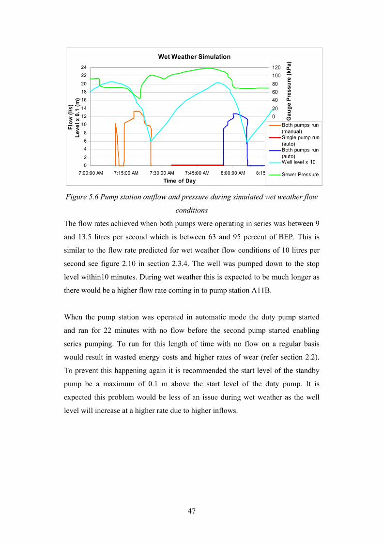
47
Wet Weather Simulation
02
4
6
8
10
1214
16
18
20
2224
7:00:00 AM 7:15:00 AM 7:30:00 AM 7:45:00 AM 8:00:00 AM 8:15:00 AM
Time of Day
Flow
(l/s
)Le
vel x
0.1
(m)
-120-100-80-60-40-20020406080100120
Gau
ge P
ress
ure
(kPa
)
Both pumps run(manual)Single pump run(auto)Both pumps run(auto)Well level x 10
Sewer Pressure
Figure 5.6 Pump station outflow and pressure during simulated wet weather flow
conditions
The flow rates achieved when both pumps were operating in series was between 9
and 13.5 litres per second which is between 63 and 95 percent of BEP. This is
similar to the flow rate predicted for wet weather flow conditions of 10 litres per
second see figure 2.10 in section 2.3.4. The well was pumped down to the stop
level within10 minutes. During wet weather this is expected to be much longer as
there would be a higher flow rate coming in to pump station A11B.
When the pump station was operated in automatic mode the duty pump started
and ran for 22 minutes with no flow before the second pump started enabling
series pumping. To run for this length of time with no flow on a regular basis
would result in wasted energy costs and higher rates of wear (refer section 2.2).
To prevent this happening again it is recommended the start level of the standby
pump be a maximum of 0.1 m above the start level of the duty pump. It is
expected this problem would be less of an issue during wet weather as the well
level will increase at a higher rate due to higher inflows.

48
5.4 Resistance to Blockage
As mentioned in section 4.3 there is a significant flow through the non running
standby pump when the pump station is operating under dry weather conditions.
To lower the risk of blockage the pump controller runs each pump with an
alternating duty. Some of the operating data of the prototype pumps from
installation (22/07/2007) to date (22/10/2007) are listed in table 5.2.
Each Pump Total
Cumulative Run Time (hours) 144 and 146 190
Number of starts 3822 and 3821 7643
Litres of sewerage pumped 6.1 million 12.2 million
Number of blockages 0 0
Table 5.2 Operating statistics for prototype pumps
From the pump station log during the same time period last year there were two
recorded blockages. This information shows that there has not been an increase in
the blockage rate up to this point. To further gauge this pump configuration’s
resistance to blockage it should be reassessed at the end of the wet season after it
has had more operating hours under all flow conditions.
5.5 Summary of Operational Testing
Testing of the series pump configuration in operation yielded favourable results.
The measured flow rate produced by the pump station exceeded the design
requirement, and the pumps operated within the desired range around the best
efficiency point (BEP). Testing of the wet weather performance was limited as
there was no rainfall during the test period. However, simulated wet weather
conditions obtained by diverting sewage flows from an adjacent catchment
showed that the pumps successfully operated in series and were able to produce
the flow rate necessary for wet weather conditions. One minor control issue arose
that caused a pump to start and run under zero flow conditions. However, that can
be addressed by adjusting the start levels of the standby pump. The pumps
operated for a total run time of 190 h in service, and no blockage problems were
encountered.

49
Chapter 6: Conclusions
6.1 Pump Station Configurations
It is common practice at Citiwater to provide pump stations discharging into
common rising mains. The pump stations have a single small fixed speed pump to
accommodate dry weather flows, and a single large fixed speed pump to provide
the additional head and flow needed for wet weather conditions. Whilst this
configuration is quite cost effective, it results in the larger pump having to run at
duty points well above and well below the best efficiency point (BEP), causing
increased energy consumption and increased pump wear.
This project considered several alternative pump configurations that would meet
design guidelines and allow the pumps to operate within the recommended range
above and below the BEP. Pump configurations considered include parallel
pumps, variable speed pumps, and series pumps. The series pump configuration
was demonstrated to have potential as an alternative arrangement compared with
current practice, and was examined in detail by theoretical analysis, design and
construction of a prototype. The prototype series pump arrangement was tested for
performance in a test tank and later installed in a working sewerage pump station.
6.2 Series Pump Configuration Suitability
Based on a particular design scenario where system resistance curves were known
for dry and wet weather, it was demonstrated that the same model pumps could
operate within their recommended operating range both as a single pump for dry
weather flow conditions and also when two pumps were connected in series for
wet weather flow conditions. Modifications could be made to two standard
submersible pumps that enabled them to operate as a single pump or to
automatically switch to work together in series when required. These
modifications were feasible and cost effective when compared to other sewerage
pump station configurations.
A series pump system was designed and constructed. Particular components
designed as part of this project included a modified auto coupling unit, pipework

50
connecting the output of one pump to the inlet of the other pump, and a non return
valve on the inlet of one of the pumps. The series pump system was installed in a
test tank and instrumented with pressure tappings and magnetic flow meters. Tank
tests were carried out over the full range of pump operation. Measured pump
curves for the individual pumps showed very close agreement with the pump
manufacturer’s performance curves. The test tank measurements showed that
there is some performance loss in connecting the pumps in a series arrangement
due to the connecting pipework and inlet non return valve. The test results
demonstrated quite good agreement between the measured and predicted
performance losses, although the measurement performance loss was less than
predicted by the mathematical model. For operation as a single unit, performance
losses due the modifications were negligible when compared to manufacturer’s
published performance curves. When the pumps operated together in series,
testing showed larger performance losses due to friction at higher flow rates. At
the flow rate required for wet weather operating conditions the performance loss
was acceptable.
The series pump arrangement has been installed in one of Citiwater’s operating
sewerage pump station since July 2007. For dry weather conditions and single
pump operation each pumps operated within its recommended operating range
both during the peak daily flow periods and for the minimum flow periods
overnight. During a simulated wet weather event the pumps operating in series
also produced flow rates that were within the recommended range. Due to a large
difference between the “start duty pump” and “start standby pump” levels it was
found the duty pump ran for an unacceptable length of time with a flow rate of
zero when under automatic control.
In the time that the pumps have been installed in the sewerage pump station no
blockages have been recorded. The series pump configuration has not shown any
increased susceptibility to blockage.
Based on the results of the tank testing and operational testing in service,
indications are that the proposed series pump configuration has successfully
achieved the goals of providing a cost effective alternative pump station

51
configuration using identical pump types. Further field testing is needed to
confirm the long term behaviour of the pumps and their reliability in comparison
to conventional installations.
The most appropriate type of pump station configuration (e.g., large and small
pumps, variable speed pumps, series pumps or other arrangement) will need to be
individually assessed during detailed design for each application, as it is
dependent on the range of system curves that will be encountered at a particular
site, and on the suitability of the available pumps.
6.3 Recommendations
It is recommended that the trial of the series pump configuration be continued and
monitored over the coming wet season to assess the performance of the station
under actual wet weather conditions.
For this type of series pump configuration the difference in height between the
“start duty pump” level and the “start standby pump” level should be as small as
practical i.e. less than 0.1 m. This is to prevent damage to the duty pump during
wet weather flow conditions caused from running for an extended period with
zero or very low flow rates.
6.4 Further Work
As the pumps have only been operating in a single sewerage pump station for
three months conclusions relating to long term reliability of the pump
configuration are not yet possible. Future work may be to install several pump
stations with the series pump configuration and monitor the pumps performance
and reliability over an extended time period and in different locations.

52
References AS 2200-2006, Australian Standard, Design charts for water supply and
sewerage, 2nd edn., Standards Australia, Sydney.
AS/NZS 4129-2000, Australian/New Zealand Standard, Fittings for polyethylene
(PE) pipes for pressure applications, Standards Australia, Sydney.
Astall, R & Rogers G 2002, Pumping Fundamentals (course notes), Strategic
Achievement, Scarborough.
AVK, 2007, Series 741/50 Flexi Check resilient seated non return valve,
brochure, Accessed at < http://www.avkvalves.com.au/>on Friday the 6th of April
2007
Citiwater 2004, Technical Services Design Guidelines, JWP, Townsville.
Fox, RW, McDonald, AT, Pritchard PJ 2004, Introduction to Fluid Mechanics, 6th
edn, John Willey & Sons, Hoboken.
Flygt, 2005, Flyps 3.1 Flygt product selection CD
Goulburn Valley Water 2007, Sewerage Pump Station Design Manual, Goulburn
Valley Water Authority, Shepparton.
Grundfos, 2007, Webcaps – Online pump selection,
Accessed at <http://www.grundfos.com/web/homeau.nsf>on Friday the 6th of
April 2007.
Sanks, RL (ed.) 1998, Pumping Station Design, 2nd. edn. Butterworth-Heinemann,
Boston.

53
Tyco Flow Control, 2007, Rubber Expansion Joints – Type FSF, Sizes 32 – 600
mm, brochure, Accessed at <http://www.tycovalves-pc.com/products.asp>on
Friday the 6th of April 2007
Tyco Water, 2007, Resilient Seated gate Valves – Figure 500, Dn80 - DN600
brochure, Accessed at
<http://www.tycowater.com/pipeline_components2/Products/>on Friday the 6th of
April 2007
WSA 02-2002, Sewerage Code of Australia, 2nd edn, Water Services Association
of Australia and Standards Australia, Sydney.
WSA 04-2005, Sewage Pumping Station Code of Australia, 2nd edn, Water
Services Association of Australia and Standards Australia, Sydney.
WSA 101-2005, Industry Standard for Submersible Pumps for Sewerage Pumping
Stations, Water Services Association of Australia and Standards Australia,
Sydney.

54
Appendices
Appendix A Project Specification

University of Southern Queensland
FACULTY OF ENGINEERING AND SURVEYING
ENG4III/41 12 Research ProjectPROJECT SPECIFICATION
Bill Weston
Design and trial of an alternative option for suburban seweragepump stations to overcome problems associated with pumpsoperating with different system curves
SUPERVISORS: Dr. Ruth Mossad, USQDr Jonathan Harris, Maunsell Australia Pty Ltd
SONSORSHIP: Citiwater, a business unit of Townsville City Council
PROJECT AIM: Typical sewage collection systems have multiple pump stationsfeeding in to a common pressure main. This project will seek toprovide an alternative pump configuration that will enable pumpsto function within their preferred operating range for differentsystem curves caused by varying demand.
PROGRAMME: Issue A,26 March 2007l. Evaluate the current pump station designs in relation to installation, operating and
maintenance costs.
Conceptual design and modelling of the alternate pump station to estimate flowsfrom pump station in both wet and dry weather systems.
Design and build experimental model of alternate pump configuration.
Test experimental model to evaluate pump system performance; calculateefficiency and losses due to friction in the added pipe work. Compare results withmathematical model.
As time permits
5. Test experimental model in sewage pump station to evaluate interaction withsystem, reliability and susceptibility to blockages.
6. Evaluate the alternate pump station design in relation to installation, operating andmaintenance costs.
reJ s t-A
FOR:
TOPIC:
2.
J .
4.
Bill Weston (Student)
Dr. Ruth Mossad (Supervisor)
Dr Jonathan Harris (Supervisor)
D^c;l..D Rer 5
/q,fu* ,qr_JJ_J"7//
f f i - -d&teL1 o?

56
Appendix B Risk Assessment Likelihood Consequence Risk Priority
Risk; New design may fail
resulting in sewage overflows to
environment
Possible Important High
(unacceptable)
New risk scores Controls;
1. build prototype and asses
in test tank
2. use pump station that if
failure occurs overflow
will be back into the sewer
network of the adjacent
pump station
Unlikely Minor Low
(acceptable)
Likelihood Consequence Risk Priority
Risk; Inhalation of poisonous
gasses from entry into the
confined space of sewage wet well
to install prototype pumps
Certain Catastrophic High
(unacceptable)
New risk scores Controls;
1. Installation to be done by
competent people
(Citiwater fitters)
2. Use of Citiwater’s
confined space procedures
Possible Minor Low
(acceptable)

57
Likelihood Consequence Risk Priority
Risk; Entry into the confined
space of sewage wet well to
service prototype pumps
Possible Catastrophic High
(unacceptable)
New risk scores Controls;
1. All service parts of
prototype must be able to
removed from well for
service.
Unlikely Minor Low
(acceptable)
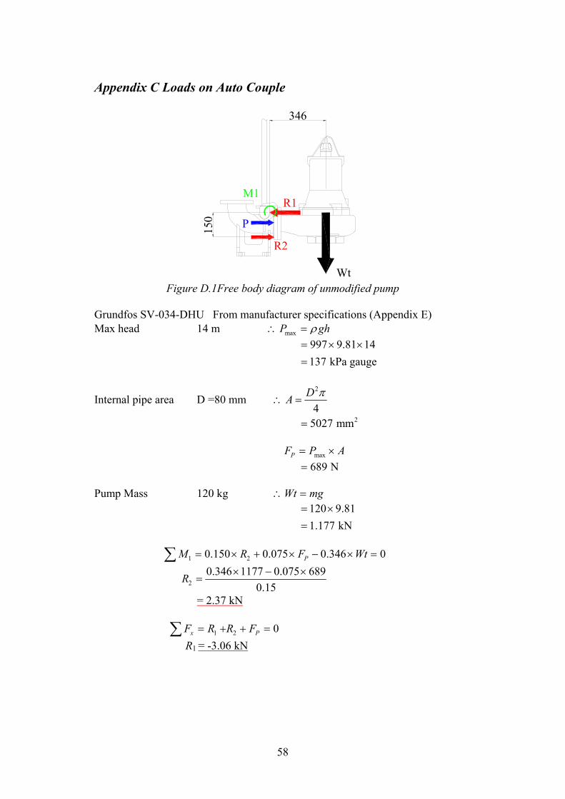
58
Appendix C Loads on Auto Couple
Wt
R1
R2
P
M1
346
150
Figure D.1Free body diagram of unmodified pump
Grundfos SV-034-DHU From manufacturer specifications (Appendix E) Max head 14 m maxP ghρ∴ =
997 9.81 14137 kPa gauge
= × ×=
Internal pipe area D =80 mm 2
4DA π
∴ =
25027 mm= maxPF P A= × 689 N= Pump Mass 120 kg Wt mg∴ =
120 9.811.177 kN
= ×=
1 20.150 0.075 0.346 0PM R F Wt= × + × − × =∑
20.346 1177 0.075 689
0.15R × − ×
=
= 2.37 kN 1 2 0x PF R R F= + + =∑ R1 = -3.06 kN

59
Wt
R1
R2
P1+P2M1
L
Figure D.2 Free body diagram of modified pump
2 12P P= P1 = 137 kPa gauge P2 = 274 kPa gauge
For both auto couples D =80 mm 25027 mmA∴ = ( )1 2PF A P P= + 2.07 kN= Estimated mass of modified pump 152 kg 1.49 kNWt∴ = To ensure load on auto couple lugs at R1 is less than unmodified version
1 6.12 kNR ≤ which is double the value of than unmodified pump as there are two auto couples. To find LMAX 1 2 0x PF R R F= + + =∑ 2 4.05 kNR∴ ≤
1 20.150 0.075 0P MAXM R F L Wt= × + × − × =∑
0.15 4050 0.075 20701490MAXL × + ×
=
= 512 mm

60
Reaction force R2 must be greater than 2.37 kN which was the calculated value from the unmodified pump.
0.15 2370 0.075 20701490MINL × + ×
∴ =
= 342 mm This value is less then the distance on the standard pump outlet Therefore to prevent overloading of modified auto couple L must be less then 512 mm. The extra pressure developed by pumping in series will not cause the auto couples to leak. 345 512 mmL∴ ≥ ≥

61
Appendix D Prototype Drawings
All design drawings were reproduced with permission from Citiwater a business
unit of Townsville City Council. All drawing completed by the Citiwater drafts
person Kevin McGrath under the direction of the author.
Appendix D1; Drawing No. CC316-01; Sewage – Garbutt Pump Station
A11B Series Pump Trial, General Arrangement
Appendix D2; Drawing No. CC316-02; Sewage – Garbutt Pump Station
A11B Series Pump Trial, Support Frame
Appendix D3; Drawing No. CC316-03; Sewage – Garbutt Pump Station
A11B Series Pump Trial, Manifold Details
Appendix D4; Drawing No. CC316-04; Sewage – Garbutt Pump Station
A11B Series Pump Trial, Discharge Manifold Details
Appendix D5; Drawing No. CC316-05; Sewage – Garbutt Pump Station
A11B Series Pump Trial, Items

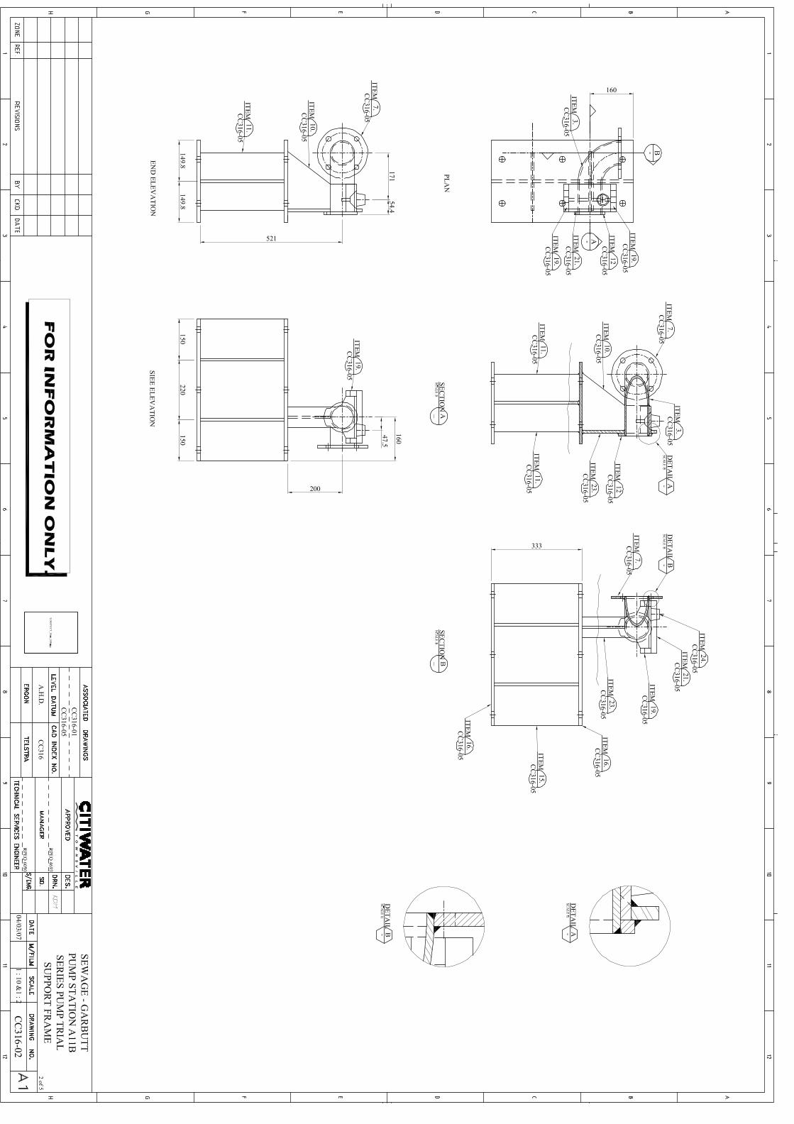


67
Appendix E, Manufacturer’s Specifications
Appendix E 1; Grundfos SV034DHU50 pump specifications
Reproduced with permission from Grundfos Australia, sourced from
Grundfos, 2007, Webcaps – Online pump selection,
Accessed at <http://www.grundfos.com/web/homeau.nsf>on Friday the 6th of
April 2007.
Appendix E 2; AVK FLEXI CHECK VALVE PN 16, brochure
Reproduced with permission from AVK Australia, sourced from
AVK, 2007, Series 741/50 Flexi Check resilient seated non return valve,
brochure, Accessed at < http://www.avkvalves.com.au/>on Friday the 6th of April
2007
Appendix E 3; Rubber Expansion Joints – Type FSF, brochure
Reproduced with permission from Tyco Pacific, sourced from
Tyco Flow Control, 2007, Rubber Expansion Joints – Type FSF, Sizes 32 – 600
mm, brochure, Accessed at <http://www.tycovalves-pc.com/products.asp>on
Friday the 6th of April 2007
Appendix E 4; Resilient Seated gate Valves – Figure 500, brochure
Reproduced with permission from Tyco Water, sourced from
Tyco Water, 2007, Resilient Seated gate Valves – Figure 500, Dn80 - DN600
brochure, Accessed at
<http://www.tycowater.com/pipeline_components2/Products/>on Friday the 6th of
April 2007

Company name:Created by:Phone:Fax:Date:
-----
-----
Printed from Grundfos CAPS
96253903 SV034DHU50
Q(l/s)0 5 10 15 20 25
H(m)
0
2
4
6
8
10
12
14
P(kW)
0
1
2
3
P2
P1
SV034DHU50
1/4

Company name:Created by:Phone:Fax:Date:
-----
-----
Printed from Grundfos CAPS
Q(l/s)0 5 10 15 20 25
H(m)
0
2
4
6
8
10
12
P(kW)
0
1
2
3P2
P1
SV034DHU50Description ValueProduct name: SV034DHU50Product No: 96253903EAN number: 5700830408711 Technical:Max flow: 101 m³/hHead max: 14 mType of impeller: SUPERVORTEXMaximum particle size: 80 mmPrimary shaft seal: SIC-SICSecondary shaft seal: SIC-CARBONCurve tolerance: ISO 9906 Annex ACooling jacket: without cooling jacket Materials:Pump housing: Cast iron
EN-JL1040 DIN W.-Nr.A48 30 AISI
Impeller: Ductile cast ironEN-JS1050 DIN W.-Nr.80-55-06 AISI
Motor: Cast ironEN-JL1040 DIN W.-Nr.A48 30 AISI
Installation:Range of ambient temperature: -20 .. 40 °CFlange standard: DINPump inlet: DN 100Pump outlet: DN 80Pressure stage: PN 10Maximum installation depth: 20 mInstallation: SInst dry/wet: SInstallation: horizontalAuto-coupling: YFrame range: 42 Liquid:Maximum liquid temperature: 40 °C Electrical data:Number of poles: 4Power input - P1: 3.6 kWRated power - P2: 2.9 kWMains frequency: 50 HzRated voltage: 3 x 400-415 VVoltage tolerance: +5/-10 %Start. method: direct-on-lineMax starts per. hour: 25I MAX: - / 7 AStarting current: 49 ARated current at no load: 4.2 ACos phi - power factor: 0,73Cos phi - p.f. at 3/4 load: 0,64Cos phi - p.f. at 1/2 load: 0,53Rated speed: 1461 rpmMotor efficiency at full load: 0,8 %Motor efficiency at 3/4 load: 0,78 %Motor efficiency at 1/2 load: 0,75 %Enclosure class (IEC 34-5): IP68Insulation class (IEC 85): FExplosion proof: noMotor protec: KLIXONLength of cable: 15 mCable type: H07RN-F AT
2/4

Company name:Created by:Phone:Fax:Date:
-----
-----
Printed from Grundfos CAPS
Description ValueCable size: 1X7X1,5MM2 Controls:Moisture sensor: with moisture sensorsWater-in-oil sensor: without water-in-oil sensor Others:Net weight: 120 kg
3/4

Company name:Created by:Phone:Fax:Date:
-----
-----
Printed from Grundfos CAPS
Note! All units are in [mm] unless others are stated.
96253903 SV034DHU50
36018
8
M16
665
120
300
R3/8
480
80
100
42
5
355
R3
805
300
ø19
600
130
665
120
520
220
15
9519
0
130 ø19
R 3/8
M16
80
840
13
11/2"
645465
345
95
160
220
M16
171
81
745
80
80
300480
1010
198
463
136
106
95
341
311
255
M16
ø19
R 3/8
100
4/4

AVK FLEXI CHECK VALVE PN 16 741/50
Flexi Check resilient seated non return valveAS 3578 dimensional complianceFlanged, drilled to AS 4087 figure B5
Use:
For potable water and sewage to max. 60°C
Tests:
Hydrostatic test to AS 4794
Seat: 16 barBody: 24 bar
Optional extras:
Bonnet plug
Materials:
Body Ductile iron, Gr. 400/12 to AS 1831 and bonnet
Resilient seated EPDM with ductile iron coredisc
Gasket EPDM rubber
Coating Fusion bonded epoxy resin to AS 4158 - Internally and externally
Bolts and Stainless steel 316 washers
The designs, materials and specifications shown are subject to change without notice due to our continuing program of product development.
AVK Australia Pty Ltd 3N74150AQ559A Grand Junction Road, Wingfield, SA 5013 Australia April 2005Tel: +61 8 8368 0900 Fax: +61 8 8368 0970e-mail: [email protected]
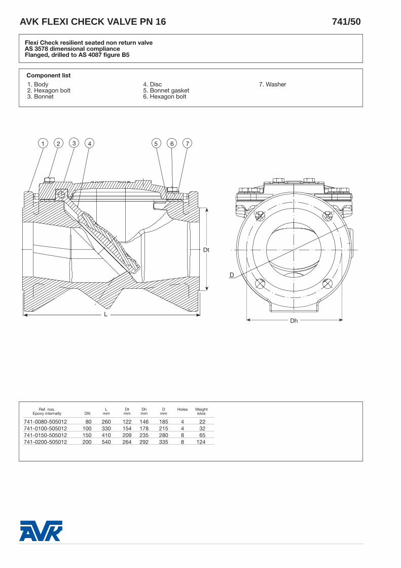
Component list 1. Body 2. Hexagon bolt 3. Bonnet
4. Disc 5. Bonnet gasket 6. Hexagon bolt
7. Washer
Ref. nos. L Dt Dh D Holes Weight Epoxy internally DN mm mm mm mm kilos
741-0080-505012 80 260 122 146 185 4 22741-0100-505012 100 330 154 178 215 4 32741-0150-505012 150 410 209 235 280 8 65741-0200-505012 200 540 264 292 335 8 124
AVK FLEXI CHECK VALVE PN 16 741/50
Flexi Check resilient seated non return valveAS 3578 dimensional complianceFlanged, drilled to AS 4087 figure B5
L
Dt
Dh
D
21 3 4 5 6 7


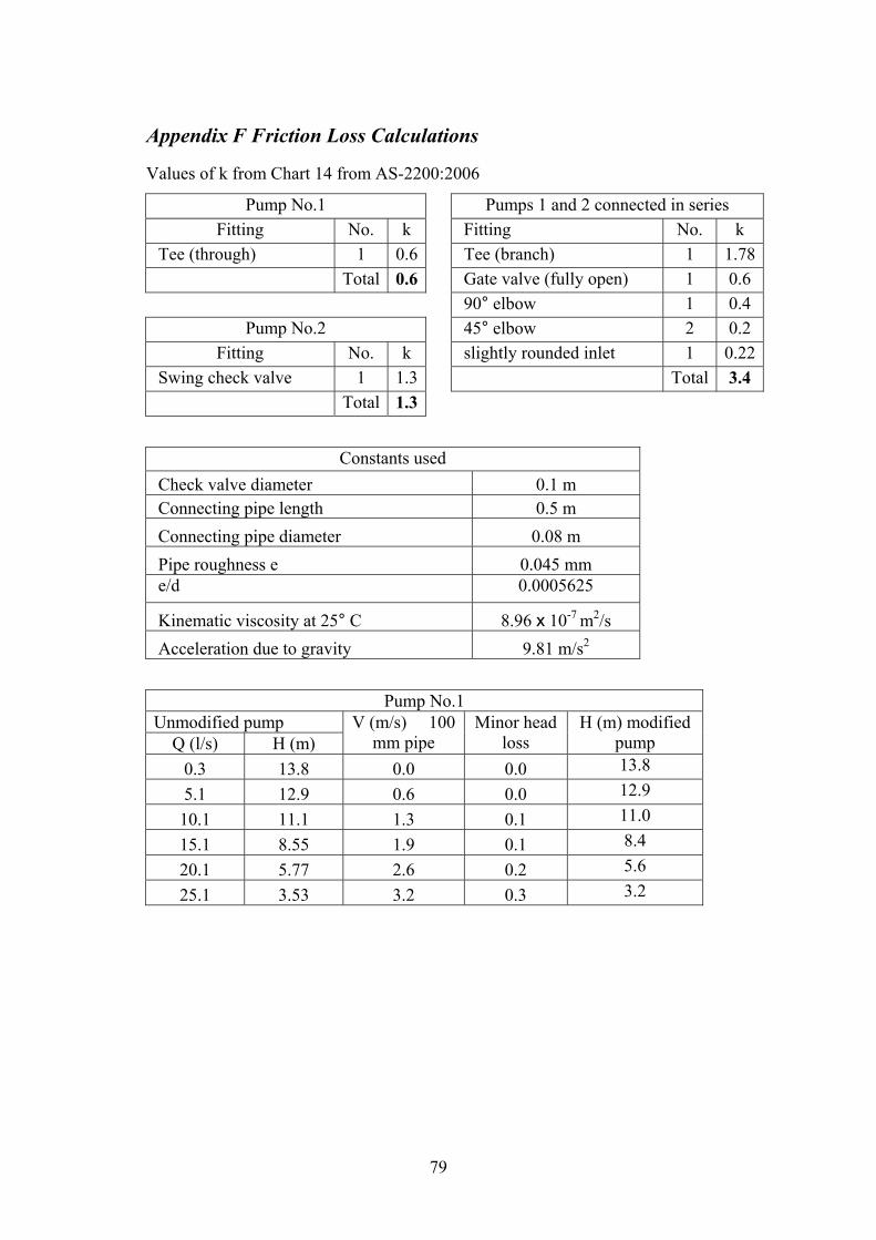
79
Appendix F Friction Loss Calculations
Values of k from Chart 14 from AS-2200:2006
Pump No.1 Pumps 1 and 2 connected in series Fitting No. k Fitting No. k
Tee (through) 1 0.6 Tee (branch) 1 1.78 Total 0.6 Gate valve (fully open) 1 0.6 90° elbow 1 0.4 Pump No.2 45° elbow 2 0.2
Fitting No. k slightly rounded inlet 1 0.22 Swing check valve 1 1.3 Total 3.4
Total 1.3
Constants used Check valve diameter 0.1 m Connecting pipe length 0.5 m Connecting pipe diameter 0.08 m Pipe roughness e 0.045 mm e/d 0.0005625
Kinematic viscosity at 25° C 8.96 x 10⁻⁷ m2/s Acceleration due to gravity 9.81 m/s2
Pump No.1 Unmodified pump
Q (l/s) H (m) V (m/s) 100
mm pipe Minor head
loss H (m) modified
pump 0.3 13.8 0.0 0.0 13.8
5.1 12.9 0.6 0.0 12.9
10.1 11.1 1.3 0.1 11.0
15.1 8.55 1.9 0.1 8.4
20.1 5.77 2.6 0.2 5.6
25.1 3.53 3.2 0.3 3.2

80
Pump No.2 Unmodified pump
Q (l/s) H (m) V (m/s) 100
mm pipe Minor head
loss H (m) modified
pump 0.3 13.8 0.0 0.0 13.8
5.1 12.9 0.6 0.0 12.9
10.1 11.1 1.3 0.1 11.0
15.1 8.55 1.9 0.2 8.3
20.1 5.77 2.6 0.4 5.3
25.1 3.53 3.2 0.7 2.9
Pumps 1 and 2 connected in series Unmodified pumps Q (l/s) H (m)
V (m/s) 80 mm
pipe
Fittings head loss
Reynold's number
f Pipe fiction
loss
H (m) modified
pump
0.3 27.6 0.1 0.001 5.33 x 10³ 0.037 0.001 27.6
5.1 25.8 1.0 0.178 9.06 x 10⁴ 0.021 0.007 25.6
10.1 22.2 2.0 0.700 1.79 x 10⁵ 0.019 0.012 21.5
15.1 17.1 3.0 1.564 2.68 x 10⁵ 0.019 0.018 15.5
20.1 11.54 4.0 2.771 3.57 x 10⁵ 0.018 0.023 8.7
25.1 7.06 5.0 4.321 4.46 x 10⁵ 0.018 0.029 2.7