DUD <aTE SCHOOL

gk ti^93943-5101

NAVAL POSTGRADUATE SCHOOLMonterey, California

THESIS

DESIGN AND PROTOTYPE DEVELOPMENT OF ANOPTIMUM SYMMETRICAL NUMBER SYSTEM

DIRECTION FINDING ARRAY

by

Panayiotis Papandreou

March 1997

Thesis Co-Advisors: Phillip E. Pace

David C. Jenn

Approved for public release; distribution is unlimited.

REPORT DOCUMENTATION PAGEForm Approved OMB No. 0704-0188

Public reporting burden for this collection of information is estimated to average 1 hour per response, including the time for reviewing instruction, searching existing data sources,

gathering and maintaining the data needed, and completing and reviewing the collection of information. Send comments regarding this burden estimate or any other aspect of this

collection of information, including suggestions for reducing this burden, to Washington Headquarters Services, Directorate for Information Operations and Reports, 1215

Jefferson Davis Highway, Suite 1204, Arlington, VA 22202-4302, and to the Office of Management and Budget, Paperwork Reduction Project (0704-0188) Washington DC20503.

1 . AGENCY USE ONLY (Leave

blank)

REPORT DATEMarch 1997

3. REPORT TYPE AND DATESCOVEREDMaster's Thesis

TITLE AND SUBTITLE TITLE OF THESIS: DESIGN ANDPROTOTYPE DEVELOPMENT OF A SYMMETRICAL NUMBERSYSTEM DIRECTION FINDING ARRAY

6. AUTHOR(S)Papandreou Panayiotis

5. FUNDING NUMBERS

7. PERFORMING ORGANIZATION NAME(S) AND ADDRESS(ES)Naval Postgraduate School

Monterey CA 93943-5000

PERFORMINGORGANIZATIONREPORT NUMBER

SPONSORING/MONITORING AGENCY NAME AND ADDRESSResearch and Development Office, Washington DC

1CSPONSORING/MONITORINGAGENCY REPORT NUMBER

1 1 . SUPPLEMENTARY NOTES The views expressed in this thesis are those of the author and do not reflect

the official policy or position of the Department of Defense or the U.S. Government.

12a. DISTRIBUTION/AVAILABILITY STATEMENTApproved for public release; distribution is unlimited.

12b.DISTRTBUTION CODE

13. ABSTRACT (maximum 200 words)

One method of estimating the direction of an electromagnetic source is based on phase comparison. In

this thesis the design and fabrication of a prototype antenna to demonstrate a new DF antenna architecture is

described. Four antenna elements are grouped into three pairs with element spacing according to a set of

symmetrical number system pairwise relatively prime moduli (ra7= 3, m2 =4, m3

= 5). The phase

difference between each pair of elements is a symmetrical folding waveform that is determined using a mixer.

The output voltage from each pair is amplitude analyzed using a small comparator ladder. In each channel, the

symmetrically folding waveform, folds in accordance with the channel modulus and thus, only requires a

precision according to that modulus. A high resolution DF is achieved after the N different SNS moduli are

used and the results of these low-precision channels are recombined to yield the direction of arrival. The

frequency of operation of the prototype is 8.5 GHz. Results based on measured and simulated data are

presented.

14. SUBJECT TERMS.Systems

Direction Finding antennas, Symmetrical number 15. NUMBER OFPAGES:

16. PRICE CODE

17. SECURITYCLASSIFICATIONOF REPORTUnclassified

18. SECURITYCLASSIFICATIONOF THIS PAGEUnclassified

19. SECURITYCLASSIFICATIONOF ABSTRACTUnclassified

20. LIMITATION OFABSTRACTUL

NSN 7540-01-280-5500 Standard Form 298 (Rev. 2-89)

Approved for public release; distribution is unlimited

DESIGN AND PROTOTYPE DEVELOPMENT OF AN OPTIMUMSYMMETRICAL NUMBER SYSTEM DIRECTION FINDING

ARRAY

Panayiotis Papandreou

Lieutenant, Hellenic Navy

B.S., Hellenic Naval Academy, 1989

Submitted in partial fulfillment of the

requirements for the degree of

MASTER OF SCIENCE IN ELECTRICAL ENGINEERING

from the

NAVAL POSTGRADUATE SCHOOL

March 1997

DUDLEY KNOX LIBRARYABSTRACT ^f-^^OOL

One method of estimating the direction of an electromagnetic source is based on

phase comparison. In this thesis the design and fabrication of a prototype antenna to

demonstrate a new DF antenna architecture is described. Four antenna elements are

grouped into three pairs with element spacing according to a set of symmetrical number

system pairwise relatively prime moduli (m;= 3, m2

= 4, m3= 5). The phase difference

between each pair of elements is a symmetrical folding waveform that is determined

using a mixer. The output voltage from each pair is amplitude analyzed using a small

comparator ladder. In each channel, the symmetrically folding waveform, folds in

accordance with the channel modulus and thus, only requires a precision according to that

modulus. A high resolution DF is achieved after the N different SNS moduli are used and

the results of these low-precision channels are recombined to yield the direction of

arrival. The frequency of operation of the prototype is 8.5 GHz. Results based on

measured and simulated data are presented.

VI

TABLE OF CONTENTS

I. INTRODUCTION 1

A. DIRECTION FINDING SYSTEMS 1

B. PRINCIPAL CONTRIBUTIONS 5

C. THESIS OUTLINE 7

II. PHASE COMPARISON DF SYSTEMS 9

A. OVERVIEW 9

B. THEORETICAL APPROACH 13

C. OPTIMUM SYMMETRICAL NUMBER SYSTEM ANTENNA 22

m. PROTOTYPE ARRAY DESIGN AND FABRICATION 33

A. OVERVIEW 33

B. MIXER DATA 35

C. LOW NOISE AMPLIFIER DATA 40

D. DESIGN OF THE ARRAY 44

E. CONSTRUCTION OF THE FIRST CHANNEL 47

F. CHECK OUT OFTHE FIRST CHANNEL 50

IV. EXPERIMENTAL RESULTS 53

A. EXPERIMENTAL SET-UP 53

Vll

B. MEASURED ARRAY RESPONSE DATA 59

V. CONCLUSIONS 63

APPENDIX A. MIXER DATA 65

APPENDIX B. LNA DATA 67

APPENDIX C. MEASURED ARRAY RESPONSE DATA 71

LIST OF REFERENCES 83

INITIAL DISTRIBUTION LIST 85

Vlll

LIST OF FIGURES

Figure 1.1: Functional elements of the direction finding process 2

Figure 2.1: Geometry of phase comparison DF 10

Figure 2.2: Phase comparison using a single-baseline antenna and a dual channel receiver

11

Figure 2.3: Linear array geometry 13

Figure 2.4: Angle of arrival vs phase difference at the elements for d = X/2 19

Figure 2.5: Phase difference at the elements vs mixer output voltage for d - X/2 19

Figure 2.6: Angle of arrival vs DC mixer output voltage for d - X/2 20

Figure 2.7: Angle of arrival vs phase difference for d = 7.5 X 21

Figure 2.8: Angle of arrival vs mixer output voltage for d = 7.5 X 21

Figure 2.9: Optimum SNS antenna architecture using moduli (ra;= 3,m2

=4) 24

Figure 2. 10: (a). Plots of the mixer outputs vs angle of arrival for the two baselines, and

(b) digitization of the plots in (a) 27

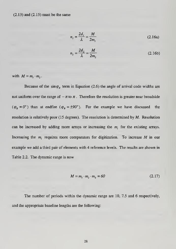
Figure 2.1 1: Plots before and after the quantization for the cases of:

(a) 3 digits / 5 X baseline,

(b) 4 digits / 3.75 X baseline, and

(c) 5 digits /3 X baseline 31

Figure 3. 1 : Block diagram of the prototype direction finding array 34

Figure 3.2: Mixer output test configuration 37

Figure 3.3: Comparison of the actual response of the mixer with the theoretical 39

IX

Figure 3.4: Input vs output power measurements for the LNAs 41

Figure 3.5: Plot of input vs output power for the four LNAs 43

Figure 3.6: Test set up for phase difference measurements of one on a branch 48

Figure 3.7: Constructed channel d = 7.5 X 49

Figure 3.8: Test of the first channel at the lab 51

Figure 4.1: LNA with a heat sink connected at the system 54

Figure 4.2: Antenna element mounted at the back side of the ground plane 55

Figure 4.3: Front side of the ground plane 55

Figure 4.4: Transmitting antenna in the anechoic chamber 56

Figure 4.5: Receiving antenna and pedestal (side view) 57

Figure 4.6: Receiving antenna and pedestal (front view) 58

Figure 4.7: Plot of theoretical vs actual results for d = 7.5 X 60

Figure 4.8: Plot of theoretical vs actual results for d = 6 X 61

Figure 4.9: Plot of theoretical vs actual results for d - 10 X 62

LIST OF TABLES

Table 2. 1 : Example of quantization of symmetrical waveforms with 2 and 3 reference

levels 25

Table 2.2: Quantization of symmetrical waveforms with 2, 3, and 4 reference levels ...29

Table A.l: Measured voltage vs phase difference for the mixer 65

Table B.l: Input power measurements vs output power for LNA 450873 67

Table B.2: Input power measurements vs output power for LNA 450874 68

Table B.3: Input power measurements vs output power for LNA 450875 69

Table B.4: Input power measurements vs output power for LNA 451376 70

Table C.l: Voltage at mixer output vs DOA measurements for d = 75X{- 90 to -39.5

deg) 71

Table C.2: Voltage at mixer output vs DOA measurements for d = 75X (- 40 to 0.5 deg)

72

Table C.3: Voltage at mixer output vs DOA measurements for d = 75X(0 to 39.5 deg)

73

Table C.4: Voltage at mixer output vs DOA measurements for d = 75X{- 40 to 89.5

deg) 74

Table C.5: Voltage at mixer output vs DOA measurements for d = 6X(- 90 to - 39.5

deg) 75

Table C.6: Voltage at mixer output vs DOA measurements for d = 6X (- 40 to - 0.5 deg)

76

XI

Table C.7: Voltage at mixer output vs DOA measurements for d = 6X (0 to 39.5 deg)..77

Table C.8: Voltage at mixer output vs DOA measurements for d = 6X (40 to - 89.5deg)

78

Table C.9: Voltage at mixer output vs DOA measurements for d = 10X (- 90 to - 39.5

deg) 79

Table CIO: Voltage at mixer output vs DOA measurements for d = 70A(-4O to -0.5

deg) 80

Table C.l 1: Voltage at mixer output vs DOA measurements for d = 10X(0 to 39.5 deg)

81

Table C.12: Voltage at mixer output vs DOA measurements for d = 70A(4O to -89.5

deg) 82

Xll

ACKNOWLEDGEMENTS

I would like to thank Professor Phillip E. Pace for giving me the chance to work

with him on this project, and for his patience, goodwill, and guidance. I also would like

to thank Professor David C. Jenn for his patience, direction, advice, and help in

constructing the antenna, and for having his door always open for me. To Bob 'Mark'

Vitale, thanks for your cooperation and help in performing the experiments, the

measurements and construction of the antenna. I learned a lot from you. To Mark Ryer,

Dave Windham, and Jason Joseph from the Radar Laboratory thank you for your help in

building the antenna. I would like to thank also the Hellenic Navy for giving me the

opportunity to come and study at the Naval Postgraduate School. Last, but not least, I

would like to thank my brothers Photis and Aris Papandreou for their help in taking the

measurements and their moral support.

This thesis was supported by the Research and Development Office, Washington

D.C.

xni

XIV

I. INTRODUCTION

A. DIRECTION FINDING SYSTEMS

A radio direction finder (RDF) is a passive device that determines the direction of

arrival (DOA) of electromagnetic energy. No transmission of electromagnetic energy by

the RDF is involved; it is a passive receiving system. It receives the incident

electromagnetic wave, processes the received signal, and thereby determines the direction

of the source. Although the radio direction finding, i.e. the use of an RDF in finding the

direction of a radio source, is only a class of direction finding, often the broad term is

used in the narrow sense.

The importance of the information provided by a direction finding (DF) system,

the emitter's bearing, is significant in several applications. For example, based on this

information the identification of a communication system or of a radar can be performed.

Also, the use of active electromagnetic counter measures (ECM) against an

electromagnetic source, requires an electronic warfare support system to measure the

direction to the victim.

A radio direction finder consists of four essential functional elements as depicted

in Figure 1.1. The antenna extracts electromagnetic energy and converts it to a signal

containing direction-of-arrival information. The receiver converts, amplifies, and

processes the signal to an intermediate frequency (IF) or baseband. The postreceiver

processor further processes the signal to obtain basic DOA information, and the DF

RDF

RF ENERGYINCIDENT AT SOME

DIRECTION-OF-ARRIVAL

v

ANTENNAWITH DIRECTIONALCHARACTERISTICS

>r

RECEIVER FORRF/IF BASEBAND

PROCESSING

>r

POST RECEIVER

PROCESSING FOR

DF INFORMATION

i f

DIRECTION-OF-ARRIVAL

INFORMATION

i '

DF INFORMATION

PROCESSING

READ-OUT DISPLAY

Figure 1.1: Functional elements of the direction finding process.

information processing-read-out-display unit prepares the basic DOA data for

transmission to users of the DF information [Ref 1].

Desirable characteristics of a DF system include: (1) wide instantaneous

bandwidth, (2) high speed, (3) minimum number of antenna elements, (4) high resolution,

and (5) wide instantaneous field of view. The antenna is a critical component of a DF

system, and frequently is the limiting factor in the system performance. It has been

difficult for traditional antenna architectures to achieve all of these attributes

simultaneously.

The DF systems are separated into three categories according to their aperture.

They are: small-aperture (or narrow-aperture), medium-aperture, and large-aperture (or

wide-aperture). Although the boundaries between them are not well specified, and some

"gray" areas occur, small-aperture systems generally have their aperture equal to half the

wavelength of the highest frequency, while the large-aperture region is considered to start

from about two times the wavelength. Medium-aperture systems are considered to start

from 0.2 to 1 .2 wavelengths.

The direction of arrival is mainly determined by one of three methods: (1)

amplitude response, (2) phase delay, or (3) time delay. In all three methods the angle of

arrival of the electromagnetic wave is converted into DC voltage, although the technique

for interpreting the voltage is different in each case.

The amplitude response method mainly uses dipole-like antenna patterns to obtain

the DF information. A radiation pattern of a dipole looks like an "eight;" it is broad at

the maximum and sharp at the minimum. By rotating the dipole it is possible to find the

direction of the emitter with a relatively high accuracy; it will be the null position, where

the voltage at the antenna terminals goes to zero. There is a 180 degree ambiguity,

because of the pattern symmetry, which can be resolved by a second antenna with a

cardioid pattern. If mechanical rotation of the dipole is not easy to accomplish, two

dipoles positioned -so as to give orthogonal patterns can be used. The values of the

electric field for the two dipoles are measured and converted to voltages which are

proportional to the sine and cosine of the incident angle, which provide angle

information.

For the phase delay method at least two separate antenna elements with a

predetermined space between them are required. Since the distances from the emitter to

the two elements are not the same (except the symmetric case), the incident wave arrives

at the two elements after traveling uneven paths, and thus it arrives with a different phase.

The phase delay is proportional to the spacing, the wavelength, and the angle of

incidence. Since the first two factors are constant, the DF information can be obtained.

Similarly the third method, time delay, uses at least two antenna elements. The

electromagnetic wave arrives at the two elements at different times. The time difference

is proportional to the distance between the antennas (which is predetermined and

constant), and the angle of incidence. Thus the direction of the emitter is obtained.

All three methods contain ambiguities and limitations, which vary for each case.

Also we have to keep in mind that the direction finding procedure is subject to several

kinds of errors, which can accumulate under certain circumstances. They include

propagation-induced errors caused by the propagation medium which introduces

deviations to the signal, environmental errors from sources in the vicinity of the direction

finder that scatter or reradiate the signal, measurement errors caused by instrument

imperfections, and observational errors.

B. PRINCIPAL CONTRIBUTIONS

This thesis is concerned with direction finders that use the phase delay method to

find the direction of an emitter. In particular, it deals with the construction of a medium

aperture radio direction finder that operates up to the frequency of 8.5 GHz and

incorporates a new signal processing approach based on symmetric number systems

(SNS). It also demonstrates how the ambiguities that occur with this method can be

overcome.

This system contains four separate antenna elements: one primary and three

secondary. The output of the primary element is mixed with the output of each of the

three secondary elements thus forming three output channels. The phase difference

between the primary and the secondary in each case is converted to a voltage. The output

phase signals are symmetrically folding waveforms that are amplitude analyzed by a

small group of comparators. In each channel, the symmetrically folding waveform, folds

in accordance with the channel modulus and thus, only requires a precision according to

that modulus. A high resolution DF is achieved after the N different SNS moduli are used

and the results of these low-precision channels are recombined to yield the direction of

arrival.

It is shown that the direction of arrival is given uniquely by the set of integer

values determined by the number of comparator threshold crossings for each modulus.

The resulting angle of arrival estimates contain quantization error, which increases with

the angle off of the electrical boresight. This is analogous to the increase in beamwidth

for an array that is scanned electronically. Several other sources of error exist: frequency

scanning error, when the emitter uses a frequency other than the design frequency, and

inaccurate comparator threshold settings.

The objective of this research is to experimentally investigate the fundamental DF

antenna concepts by building a prototype and measuring its performance in the anechoic

chamber. To reduce cost, off-the-shelf in-house hardware is used in the array. Therefore,

the array performance is not the optimum, but the array can be used to validate the

important SNS DF concepts. A simple narrow band radiating element is used. The SNS

DF antenna is designed for use with an existing comparator and encoding hardware

developed on a previous research program.

The wide-band performance of the array is primarily determined by the radiating

element design, which will not be addressed in this research. All of the fundamental

concepts can be demonstrated using narrow band elements. They include: (1) microwave

beamforming network design and the performance requirements of its components

(mixers and amplifiers), (2) DF resolution as a function of angle, (3) effect of the element

factor and signal-to-noise (SNR) level on DF accuracy, (4) resolution versus boresight,

(5) interface between each channel's phase response and the corresponding amplitude

analyzing hardware, and (6) verification of frequency compensation and interpolation

methods to maintain high resolution.

C. THESIS OUTLINE

The thesis presents the theoretical background and the design equations needed to

construct a large aperture radio direction finder based on a symmetric number system. A

DF array was fabricated, assembled and measured in the anechoic chamber. The

measured data verified the fundamental concept and performance of the new SNS DF

approach.

Chapter II presents a theoretical background in direction finders using the phase

difference between antenna elements for direction of arrival information. A design for a

8.5 GHz four-element array is presented. Chapter EI describes the actual design and the

fabrication of the direction finding system. It begins with the process of component

evaluation in the lab. Individual antenna components such as the mixers and the low

noise amplifiers were measured on the network analyzer so that differences in their

phases and amplitudes could be compensated for in the actual design. Next the design

and assembly of the system follows. This includes phase trimming and checkout in the

lab. A plane wave was simulated by exciting both branches with equal amplitude signals

that had known phase differences to verify the assembly before proceeding to the

chamber. Chapter IV presents the experimental anechoic chamber results, and Chapter V

states some conclusions and recommendations for future research.

II. PHASE COMPARISON DF SYSTEMS

A. OVERVIEW

Phase comparison DF systems consist of several antenna elements which are

arranged in a particular geometrical configuration. The number of the elements and

arrangement depends on the DOAs of interest and the method used to process the signals.

However, the minimum number of elements is two. The determination of DOA is

performed by direct phase comparison of the received signals from the different antenna

elements.

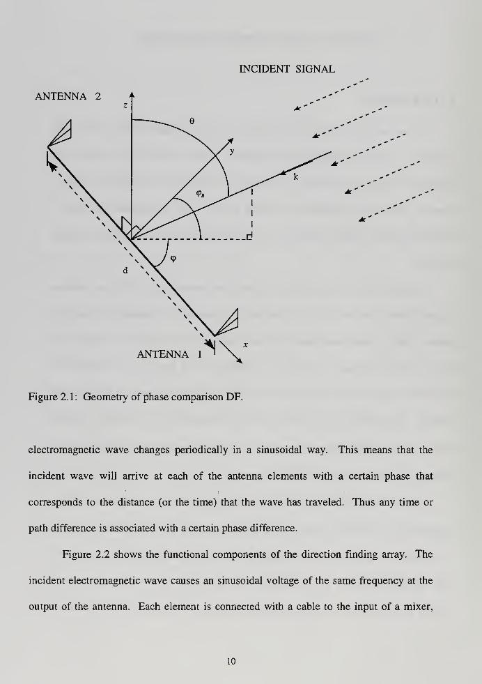
Figure 2.1 shows the geometry of a typical two element system. The two antenna

elements define a line, here the x-axis, and they are separated by a distance d, the baseline

spacing. The x-y plane corresponds to the earth's surface for a ground based system, with

the z axis the vertical axis. The source is assumed to be far away, so the wavefronts of

the incident signal are planar, and the wave arrives at the same angle at both antenna

elements. The bearing of the incident wave (pB , is measured in the horizontal x-y plane

from the v axis, while the elevation angle 6 , which for the general case is not 90 degrees,

is measured from the z axis towards the x-y plane.

For a linear array, only for the case where cpB= does the incident wave arrive at

the same time at all antenna elements. For all the other cases the wave arrives at different

time instances at the two antenna elements due to unequal paths from the source. This

time difference of arrival is a function of the angle cpB . Therefore, every horizontal

bearing cpB is related to a certain time or path difference. Also, the phase of a traveling

INCIDENT SIGNAL

ANTENNA 2

ANTENNA

Figure 2. 1 : Geometry of phase comparison DF.

electromagnetic wave changes periodically in a sinusoidal way. This means that the

incident wave will arrive at each of the antenna elements with a certain phase that

corresponds to the distance (or the time) that the wave has traveled. Thus any time or

path difference is associated with a certain phase difference.

Figure 2.2 shows the functional components of the direction finding array. The

incident electromagnetic wave causes an sinusoidal voltage of the same frequency at the

output of the antenna. Each element is connected with a cable to the input of a mixer,

10

which operates as a phase comparator. With equal cable lengths the two signals arrive at

the input of the mixer with the free space (plane wave) phase difference. At the mixer the

two AC voltages are multiplied and at the output they produce a voltage which is a

function of the phase difference of the incident wavefront. Thus an azimuthal angle of

ANTENNA 2 ANTENNA 1

DUAL-CHANNELRECEIVER

V

PHASEDETECTOR

A\|/

BEARINGCOMPUTATION

<P

INCIDENTWAVE

Figure 2.2: Phase comparison using a single-baseline antenna and a dual channel

receiver.

11

incidence <pB causes a certain time (or distance-traveled) difference between the two

antenna elements, and equivalently a certain phase difference between the two elements

that corresponds to a certain voltage value, which is measured.

In order to have unambiguous AOA estimates from -90 to +90 degrees, the phase

difference must correspond to a range of -k to n radians. Having q>B equal to 90

degrees means that the wave travels parallel to the baseline of the two elements, and

therefore d is the additional distance to reach the second element. In order to arrive there

with a phase difference of n radians d must be equal to half of a wavelength.

Although this approach avoids the ambiguity problem, there is a tradeoff: there is

a limit to resolution, because the 180 degree range of possible source bearings cannot

exceed 2n radians of phase difference. There is also a second consideration. The

distance between the two elements is going to be half the wavelength this means that for

the frequency of interest, 8.5 GHz, this distance is about 1.76 cm. This is too close for

most types of radiating elements. A better approach is to place the antenna elements at a

distance equal to a multiple of the half the wavelength, and then use multiple arrays with

different spacings to resolve the ambiguity.

Estimating the elevation angle 6 is a separate issue. For a single baseline system

all elevation angles give the same antenna response, and thus it is not possible to

determine 6 . The elevation angle can be determined with the use of a second baseline, if

the second pair of elements is placed orthogonal to the first, i.e. along the vertical axis.

This yields a set of two independent measurements, which correspond to the two angles

q>B and 6 . However, the estimation of 6 will not be a subject of this thesis. In this case

we restrict both the antenna and the signal source to lie in the x-y plane.

12

B. THEORETICAL APPROACH

The purpose of this section is to present the mathematical approach and derive the

equations that relate angle of incidence with phase difference at the elements to the

voltage at the output of the mixer. Figure 2.3 shows the geometry of the problem. As

INCIDENT n

PLANE WAVE^

ANTENNA 2

Figure2.3: Linear array geometry.

13

mentioned previously, the elevation angle is 90 degrees and we consider only waves

arriving in the x-y plane. There are two antenna elements with distance d, and the plane

wave travels with incidence angle cpB . The angle (pB is measured from the perpendicular

to the baseline axis and it takes values from +nl2 to - nil. Note that cpB is related to the

spherical polar angle (p by:

K% = 2~<P

Let k be the unit vector of the direction of wave propagation. Then

A A

k = -(x-cos(p+ v-sin<p) (2.1)

The instantaneous electric field propagating toward the array in free space is given by the

following formula:

E(t,k) = z-E -cos(27tft-Pr) (2.2)

where : E is the maximum value of the electric field,

/ is the frequency

(5 is the phase constant (or wave number)

r is the distance traveled from source

14

(3r = -p(xsm(pB +y-cos(pB )

and we assume that the wave is vertically polarized. The phase constant (5 is equal to

n 2kP =

-J(2.3)

where X is the wavelength. This last relationship implies that for every wavelength of

distance traveled, an equiphase plane undergoes a phase change of 2k radians.

The electromagnetic wave arrives first at the element 1. This element is located at

dx = —and y = . Without affecting the general case, we can assume that the phase of the

wave arriving there at time t is

Wi = 2nft (2-4)

The wave arrives at element 2 after traveling an additional distance of d-s'm(pB . Its

phase is

2ky/2

= 270 -— d sin (pB (2.5)A

From (2.4) and (2.5), the phase difference between the two elements is:

15

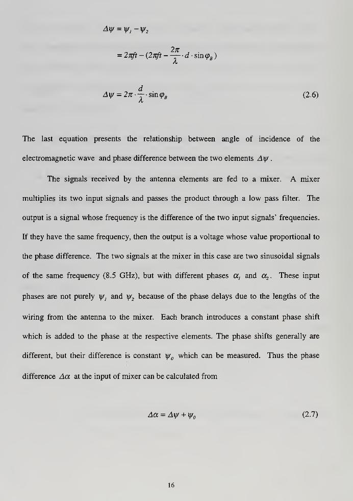
AV = Yi-Y2

2n= 27Tft - (270 -— • d • sin <pB )

dAy/ = 2n;—-sm(pB (2.6)

A

The last equation presents the relationship between angle of incidence of the

electromagnetic wave and phase difference between the two elements Ay/

.

The signals received by the antenna elements are fed to a mixer. A mixer

multiplies its two input signals and passes the product through a low pass filter. The

output is a signal whose frequency is the difference of the two input signals' frequencies.

If they have the same frequency, then the output is a voltage whose value proportional to

the phase difference. The two signals at the mixer in this case are two sinusoidal signals

of the same frequency (8.5 GHz), but with different phases a, and a2. These input

phases are not purely y/j and y/2 because of the phase delays due to the lengths of the

wiring from the antenna to the mixer. Each branch introduces a constant phase shift

which is added to the phase at the respective elements. The phase shifts generally are

different, but their difference is constant y/ which can be measured. Thus the phase

difference Aa at the input of mixer can be calculated from

Aa = Ay/ + y/ (2.7)

16

Alternately, if we choose the length of the cable to be equal for both branches, Aa = Ay/ .

The latter approach of equal paths is preferred, but sometimes is not possible to achieve

because of the circuit layout constraints.

The two inputs of the mixer are of the form

v1(t) = V-cos[27tft + a

1(t)] (2.8a)

v2(t) = V-cos[27rft + a2

(t)] (2.8b)

where, V is the maximum value of the voltage at the element terminals due to the

incident wave, and / is the frequency of 8.5 GHz. Before low pass filtering the

instantaneous mixer output voltage is

vaBt

/

(0 = v;(0-v2 (0

voJ (0 = V2

cos[27i/r + a}(t)] • cos[27tft + a2 (*)]

V 2

vj(t) =— {cos[4jrft + a, (t) + cc2(r )] + cos[a

7(r) - a2 (f)]

}

(2.9)

The low pass filtering removes the high frequency term on the right hand side of (2.9)

leaving

V 2

17

V 2

vout

(t) =— -cos(Aa)

V 2

vout

{t) =— -cos{ A\if) (2.10)

which is the required voltage. Equation (2.10) presents the relationship between the

mixer voltage output v0UJ

and phase difference at the elements. Combining equations

(2.6) and (2.10) gives

V 2 dvOM (t) =— -cos[2K---s™(<PB )'\ (2- 11 )

Equation (2.1 1) is the relationship between voltage at the output of the mixer and angle of

incidence of the electromagnetic wave.

From Equation (2.6) it is apparent that if the baseline d is half the wavelength X or

less, the phase difference is between -n and k. For every value of phase difference there

is only one unique angle of incidence. In this case no ambiguities exist. With distance

between the two elements half the wavelength, the phase difference is

Ay = n-sm{(pB ) (2.12)

and it is plotted in Figure 2.4. Figure 2.5 shows the plot of Equation (2.10); the

voltage versus phase difference. Note that this plot is independent of the baseline length

o

<D

15>>—

CO*•—

oo

c<

100

50

0_

-50

100

1

1

\

i

—I

1

r

i

-r

i

i

i

... _1 .

1

DO -150 -100 -50 50 100 150 20

Phase difference (degrees)

XFigure 2.4: Angle of arrival vs phase difference at the elements for d = —

.

300

200.

£ 100

D5CO

-200.

-300-200 -150 200

Phase difference (degrees)

Figure 2.5: Phase difference at the elements vs mixer output voltage for dX

19

and is the same for every baseline. For every voltage value there are two possible phase

differences: y/ and -y/. Figure 2.6 is a direct combination of the curves in Figures 2.4

and 2.5; it is the plot of voltage versus angle of incidence. For every value of voltage we

have only two possible values of angle of incidence. This ambiguity can be eliminated by

using a second array with a baseline that is not an integer multiple of the first.

300

-100 -80

Angle of incidence (degrees)

100

Figure 2.6: Angle of arrival vs mixer output voltage for d = —

.

For baselines greater than half the wavelength more ambiguities exist, since the

phase difference takes on multiple values outside of the interval -n to n, and thus

corresponds to more than one angle of incidence. Figures 2.7 and 2.8 show the data for a

baseline d equal to 7.5 times the wavelength. The rapid change in voltage with phase

20

CO0)CD1—

O)<D

>1—

CO

o

c<

100

50.

-50.

-100_-200 -150

Phase difference (degrees)

200

Figure 2.7: Angle of arrival vs phase difference for d = 75X

.

300

200 _

CO 100o>FQJTOCO*—

*

O> -100

-200

-300-100 -80 -60 30 -20

—-20

Angle of arrival (degrees)

60 80 100

Figure 2.8: Angle of arrival vs mixer output voltage for d = 7.5X

.

21

difference allows higher resolution AOA estimates. The tradeoff is that the voltage is

highly ambiguous; 15 angles of incidence correspond to every value of phase difference,

and 30 angles of incidence to every value of voltage. The number of periods n that

correspond to 180 degrees in a voltage versus angle plot is

2dn =— (2.13)

Figure 2.8 illustrates that the voltage period is not constant when plotted as a

function of angle. The period increases with the increase of DOA from the array

broadside {(pB =0) because of the s'm(pB dependence in Equation (2.6). This is the same

reason that the beamwidth of an electronically scanned phased array increases with scan

angle.

C. OPTIMUM SYMMETRICAL NUMBER SYSTEM ANTENNA

The optimum SNS scheme is composed of a number of pairwise relatively prime

(PRP) moduli m,. The integers within each SNS modulus are representative of a

symmetrically folded waveform with the period of the waveform equal to twice the PRP

modulus, i.e., 2m, . For m given, the integer values within twice the individual modulus

are given by the row vector

xm =[0,l,...,m-l,m-l,...,l,0].

22

From this expression, the required number of comparators for each channel is ra, -1. Due

to the presence of ambiguities, the integers within the vector do not form a complete

system of length 2ra by themselves. The ambiguities that arise within the modulus are

resolved by considering the paired values from all channels together. By recombining the

;V channels, the SNS is rendered a complete system having a one-to-one correspondence

with the residue number system (RNS). For N equal to the number of PRP moduli, the

dynamic range of this scheme is

M = Umi

N

[Ii=7

This dynamic range is also the position of the first repetitive moduli vector. For the

example of m, = 4 and m2= 3 , the first repetitive moduli vector occurs at an input of 12

[Ref6].

The ambiguity problem observed in Figure 2.8 can be eliminated by the

simultaneous use of more than one pair of antenna elements with differing baselines of

several wavelengths depending upon the modulus with each pair forming a separate

receive channel. The output of each channel or modulus is amplitude analyzed by a small

ladder of comparators. The channels are recombined and the result is a high accuracy

unambiguous estimate of the DOA.

Consider the case of two pairs of antenna elements with different baselines. The

plots of the voltage at each mixer output versus angle of arrival is a sinusoid. In order to

23

convert these analog signals to digital codes, they are quantized with respect to predefined

reference levels (see Figure 2.9). Each level represents an integer value within the

modulus. The number of possible digits m is the number of the reference levels n plus

one. If the first signal is quantized with two reference levels and the second with three,

they are converted to the two strings shown in Table 2.1.

V V Vdj

PHASE DETECTOR

PHASE DETECTOR

m=3

m=4

COMPARATORS

SNSTODECIMALLOGICBLOCK

„<PB

Figure 2.9: Optimum SNS antenna architecture using 2 moduli (m, = 3 ,m2=4).

24

m, = 3 m2=4

Angle Interval 3 digits / 2 reference levels 4 digits/3 reference levels

1

2 1 1

3 2 2

4 2 3

5 1 3

6 2

7 1

8 1

9 2

10 2 1

11 1 2

12 3

13 3

Table 2.1: Example of quantization of symmetrical waveforms with 2 and 3 reference

levels.

The entries in Table 2. 1 are the possible values that an incoming signal produces

at the output of the comparator ladder for each baseline. They are periodic with different

periods for each case (period is 2mi). If they are viewed as pairs, the first twelve of them

are unambiguous: none of them appears twice. Note that this number is the product of

25

the possible digits m, for the two cases ( M = m1m2

= 3-4 = 12), and is called dynamic

range. If within the dynamic range both plots cover exactly 180 degrees, then each table

entry corresponds to a 15 degrees interval. Thus, by knowing the two digits we know the

angle of arrival. However, since the voltage is quantized, the DOA estimate is also

quantized. Therefore the DOA can only be determined with a certain resolution. The

difference between the estimate and the true DOA is the quantization error.

Within the dynamic range the first column of integers has n}= 2 periods, while

the second has n2-SI2. From Equation (2.13) the required spacings for the

unambiguous DOA estimates are

rij

dj =— A = A

(2.14)

d7=—A = 075-A2

2

Thus, two pairs of elements with these baselines having two and three quantization levels,

respectively, yield unambiguous angle of arrival estimates with a resolution of 15°

.

Figure 2.10 shows the voltage at the mixer outputs for the two arrays versus angle of

arrival, before and after quantization. All the resulting pairs of digits are unique. The

above example has demonstrated that we can obtain unambiguous results if we use two

arrays with the appropriate combination of spacings and quantization levels. The number

of periods within the dynamic range is given by the following equation:

26

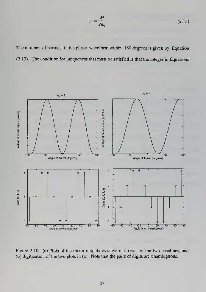
n. —M2m:

(2.15)

The number of periods in the phase waveform within 1 80 degrees is given by Equation

(2.13). The condition for uniqueness that must be satisfied is that the integer in Equations

m, = 3171^=4

TOOAngle of Arrival (degrees) Angle of Arrival (degrees)

Q l

-80 30" 3o" 3C 6 & #5 5*5 5

Angle of Arrival (degrees)

SC 3<3 3*5 3o~ 3 25 40 60 80Angle of Arrival (degrees)

Figure 2.10: (a) Plots of the mixer outputs vs angle of arrival for the two baselines, and

(b) digitization of the two plots in (a). Note that the pairs of digits are unambiguous.

27

(2.13) and (2.15) must be the same

2d, Mnj=-T =T~ <2 - 16a)

a zrrij

2d2 M••—x-s: (2 - 16b)

with M = m,m2.

Because of the sin<pB term in Equation (2.6) the angle of arrival code widths are

not uniform over the range of - n to n . Therefore the resolution is greater near broadside

( cpB=0°) than at endfire ( cpB

= ±90° ). For the example we have discussed the

resolution is relatively poor (15 degrees). The resolution is determined by M. Resolution

can be increased by adding more arrays or increasing the mi

for the existing arrays.

Increasing the mi

requires more comparators for digitization. To increase M in our

example we add a third pair of elements with 4 reference levels. The results are shown in

Table 2.2. The dynamic range is now

M = m, • m2

• m3= 60 (2.17)

The number of periods within the dynamic range are 10, 7.5 and 6 respectively,

and the appropriate baseline lengths are the following:

28

rtij = 3 m2=4 m

3=5

Angle interval 3 digits/ 2 ref. levels 4 digits/3 ref.levels 5 digits/ 4 ref. levels

1

2 1 1 1

3 2 2 2

4 2 3 3

5 1 3 4

6 2 4

7 1 3

8 1 2

9 2 1

10 2 1

11 1 2

12 3 1

13 3 2

14 1 2 3

15 2 1 4

: : : :

58 2 1 2

59 1 2 1

60 3

Table 2.2: Quantization of symmetrical waveforms with 2,3, and 4 reference levels.

29

2d, n, „

n]=—L ^>d

] =-r-A=5h (2.18a)A 2

2d7 n7 „n2=^-=>J

2 =-r--A = 375A (2.18b)A 2

2d, n, „

n1=^rL =>d

]=-±-X=>d

]=3X (2.18c)

A 2

Figure 2.11 shows the plots before and after the quantization for the three cases. Since

the 180 degrees are divided to 60 intervals, the resolution is 3 degrees at broadside. As

Equations (2.16) suggest, the desired resolution can be achieved with several different

combinations. Resolution is a tradeoff between number of arrays (element pairs) and

number of quantization levels (comparators).

30

o>E

sin (Angle of Arrival)

sin (Angle of Arrival)

sin (Angle of Arrival)

i p go go co 99 90 99 o

© co do do co so do do

TOO -160 30~ "56" 7Q0

sin (Angle of Arrival)

SB co OB co QD 99

CO CO CO CO

iosr

sin (Angle of Arrival)

^55 5 5o~

sin (Angle of Arrival)

TOO

Figure 2.11: Plots before and after the quantization for the cases of (a) 3 digits / 5 Abaseline, (b) 4 digits / 3.75 A baseline, and (c) 5 digits / 3 A baseline.

31

32

in. PROTOTYPE ARRAY DESIGN AND FABRICATION

A. OVERVIEW

The block diagram of the prototype DF array beamforming network and signal

processor is presented in Figure 3.1. It consists of three separate two-element arrays that

sample the incident wavefront and mix the signals from the two branches. In this

particular design there are four antenna elements. Element one is referred to as primary

and is shared by all pairs. The other three elements are spaced at non integer multiples of

a half wavelength. The distances are determined by the SNS that will be used to encode

the angle data. In this case the moduli m7=3, m2

= 4, and m3= 5 are used because of

the availability of existing SNS digital processing hardware.

Each channel, in addition to the two antenna elements, also contains two low

noise amplifiers (LNAs) and a mixer. The amplifiers are used to boost the incident signal

up to the operational range of the mixers. The mixer multiplies the two inputs, as

described by Equation (2.9) and low-pass filters the output so that only the baseband

phase component is present at the output. This voltage, whose level is proportional to the

phase difference between the two inputs, is then passed to the SNS digital processor. The

SNS digital processor first amplitude analyzes the phase response within each channel

and then recombines these results in a logic block that produces the DOA, as described in

the Section C of Chapter n.

33

¥LNA

V V VLNA LNA

LPF

LPF

LPF m=3

m=4

m=5

LNA

>>

Figure 3.1: Block diagram of the prototype direction finding array.

SNSTODIGITALBLOCK

<Pi

The objective of this thesis is to design and construct a three array SNS DF

antenna and verify its performance at 8.5 GHz by taking pattern measurements in the

anechoic chamber. As a first step, the performance of the individual antenna components

34

are determined. The analysis has assumed ideal device characteristics, and any deviation

from the non-ideal case must be compensated for in the design and assembly of the

antenna. The performance of each component is determined using a network analyzer.

The quantities of interest are the scattering parameters, or equivalently the reflection and

transmission coefficients at both device ports. For the mixers, we are interested in the

phase difference versus output voltage, while for the LNAs it is the input power versus

output power relationship. Note that the knowledge of the phase is necessary for correct

assembly of the beamformer.

An important step is the calculation of the appropriate length of the coaxial cables,

and their fabrication. They must be adjusted to avoid any unwanted phase differences

between the antenna elements and the mixer. The cable lengths are also used to shift the

output phase response curves so that a minimum value occurs at (pB= -90° for all

channels. When constructed in the lab the cables insertion phase may only be within

± 5° of the required phases. The remaining error is corrected by using adjustable phase

shifters. Next, each channel gets assembled and tested in the lab under similar conditions

to those expected in the chamber. That is, pairs of elements are excited with equal

amplitude phase-shifted waves to simulate an incident plane wave. Finally, data is

collected in the anechoic chamber.

B. MIXER DATA

In Chapter II we presented the operation of a mixer and we derived the formula

that relates its output voltage to the phase difference of its inputs:

35

2vout(t)=—-cos(Aa) (3.1)

This is the ideal result; an actual mixer will deviate from this. Furthermore the mixers are

not identical, i.e., there will be variations in the DC output level for similar signals at

their inputs. It is necessary to test the individual mixers and record the differences in

performance so that they may be accounted for in the design. The approach is to create a

signal of 8.5 GHz and send phase shifted versions of it through cables to both inputs of

the mixers. Phase differences were obtained with phase shifters in one branch, thus

simulating a plane wave excitation at the mixer input. The test setup includes a network

analyzer with its signal generator, a power splitter, two phase shifters, and a voltmeter as

shown in Figure 3.2.

Semi-rigid coaxial cables were used to make connections to the mixers so that

phase stability could be maintained. Since these cables are not flexible, they have to be

constructed and laid out in such a way as to fit between the radiating elements and

mixers. The vector network analyzer generated a signal of 15 dBm. Although this signal

is less than that expected in the chamber, it was the maximum possible from the analyzer.

The signal was passed through a power splitter yielding two identical signals at half of the

incident power. Each signal was sent to a mixer input. The branches included phase

shifters to introduce a phase shift. One branch included a 10 dB directional coupler to

serve as a reference. The -10 dB output of the coupler was connected to the network

36

analyzer. The circuit also included several different adapters and barrels to interconnect

different types of cables and components.

Voltage measurements were taken from a voltmeter connected at the output of the

mixer. Phase measurements should normally be measured directly at the input of the

mixer. Unfortunately there was no way to measure the phase at these points without

disconnecting the mixer every time. This is not only tedious and time consuming, but

also reduces the accuracy of the phase measurements. Connecting and disconnecting

components, moving or slightly bending cables, and connector torque can cause

2.4Female

to 3.5Male

Adaptor / Power Splitter

3.5Female to N Male

Adaptor

Figure 3.2: Mixer output test configuration.

37

variations in phase shift. Phase measurements were taken from the vector network

analyzer between the input of the power splitter and the -10 dB output of the coupler. To

be precise they were taken between the 3.5-female-to-N-male adapter and the male-to-

male-barrel. The presence of these components cause a phase shift which also has to be

taken into account. Figure 3.2 shows the test points of the measurements.

A reference phase was obtained by measuring the phase difference between

points A and B of Figure 3.2, and their respective mixer inputs C, D and then

subtracting it out to get the desired phase difference. The phase reference point was

chosen as the input of the 3.5-female-to-N-Male adapter where the first port of the vector

network analyzer was connected (A). The phase difference between this point and the

output of the phase shifter at the first branch (C) was found to be -57.1 degrees. For the

second branch the output of the male-to-male-barrel after the -10 dB output of the coupler

(B) had a phase difference of -168.3 degrees, while at the barrel before the mixer at point

D (with the -10 dB output of the coupler matched) was 150.4 degrees. The measured and

computed phase differences (in degrees) are:

AB = -57.1

AD = 150.4

AC = 168.63

BD=AD- AB =150.4 - (-57.1) = 207.5

CD=AD-AC = AB + BD -AC = AB + 207.5 -168.63 = AB + 38.87

38

For every phase measurement taken it was necessary to add 38.87 degrees to refer it to the

phase difference at the input of the mixer.

Phase shifters were used to change the phase, which was recorded at the network

analyzer, and the output voltage at the voltmeter. The results are presented at Table A. 1

in Appendix A, and a plot shown in Figure 3.3. The gray line shows the theoretical

result. The comparison of the two shows that the general behavior of the mixer was as

expected. The differences are within the measurement accuracy of the test set-up.

-200 00 -50 50 10phase difference (degrees)

150 200

Figure 3.3: Comparison of the actual response of the mixer with the theoretical.

39

C. LOW NOISE AMPLIFIER DATA

Low noise amplifiers (LNAs) are used in radar and direction finding systems to

increase signal level without introducing significant noise. Therefore, they not only

increase the signal power level, but also to improve the signal-to-noise ratio (SNR).

The antenna receives both signal and noise. Also every component in the receive

channel contributes thermal noise, which adds to the total noise. Components like mixers

SNR.have a high noise figure F, where F = ——— . LNAs on the other hand introduce little

noise, yet amplify the signal such that the SNR is increased. The noise introduced by a

mixer can be several times the noise of the LNA, but because the SNR was increased by

the LNA its effect on the total signal-to-noise ratio is negligible. A typical noise figure

for an LNA is around ldB.

LNAs can introduce signal distortions. The power input to power output response

is not linear and eventually the output power will saturate. Also, the phase shift vs

frequency can be different for every individual LNA depending on its construction, which

cannot be predicted and has to be measured. The linear and the saturation ranges are

important to know for proper operation of the antenna.

In the array, the low noise amplifiers are to be connected between the antenna

elements and the mixers. The amplifiers will be operated in the saturation region so that

the output power level remains constant for the expected variation in input level.

According to Equation (3.1) the voltage level at the output of the mixer depends not only

on the phase difference but also on the maximum voltage level of the mixer's input

signals. If the amplifiers were not included, the maximum voltage level would drop off

40

with angle from boresight due to the element factor. The output of the mixer would be

dependent on the signal strength, and the DC signal would not be a constant amplitude

sinusoid. Sources at different angles, would create different voltage levels at the mixer

output, even if they were at the same range. Operating the LNAs in the saturation region

alleviates this problem. The LNAs were manufactured to be phase matched within 10

degrees.

To determine the operating characteristics of the LNAs, a signal generator and

two power meters were used as shown in Figure 3.4. The signal generator was connected

Power GeneratorDC Volts

r+15)

Directional

coupler

T=r

-20dB

LNA

Power

Meter

-k:

Power

Meter

Figure 3.4: Input vs output power measurements for the LNAs.

41

to a - 20 dB directional coupler. A power meter connected at the -20 dB output was used

measure the input power level. The LNA was connected to the through port of the

coupler and the second power meter was connected to the output of LNA to measure the

output power level. A DC voltage source of 15 volts was connected to the LNA to

activate it. Also a heat sink was attached to the LNA to ensure that heat damage would

not occur. At this point phase was not measured, first because the LNAs were ordered to

be phased matched, and secondly, the phase difference of the entire branch will be

measured before final assembly. For these measurements the input power level was

increased and the output power level recorded. A problem that we faced was that the

output did not settle down immediately, but there were some fluctuations and it was

necessary to wait considerably to get a stable reading. This in turn increased the problem

of overheating of the LNAs.

The determination of the input power range used for the measurements was based

on the hardware limitations. The signal generator had a maximum power output of - 9

dBm. Thus this value determined the maximum signal power value used. On the other

hand the power meter input had a minimum sensitivity of - 60 dBm. Since the signal to

the power meter was passing through the - 20 dB arm of the coupler, the minimum value

of the signal before the coupler that would be detected was - 40 dBm. This input power

range of - 40 dBm to - 9 dBm was adequate for our purposes. Because of the coupler,

every measurement value taken from the power meter had to have 20 dB.

42

10

£CD

2,i_

OQ.+->

3Q.

o

^J-PH-1 1 1I " ++

5Spli

J^ 450873: +

rfx 450874:*

2$* 450875: o

-5J| 451376:-

-10- Jft*

-15r

i i i i

-40 -30 -20 -10

Input power (dBm)10

Figure 3.5: Plot of input vs output power for the four LNAs.

Figure 3.5 present the plots of input power versus output power for the four

LNAs. Tables B.l through B.4 in Appendix B present the raw data. From Figure 3.5 we

can see that the curves are matched and initially linear up to about - 28 dBm input power.

After -20 dBm they saturate. There are some minor differences in the curves between the

amplifiers, although these differences are not expected to influence the DF performance.

43

D. DESIGN OF THE ARRAY

The first task in the design of the array is to calculate the distance between the

element pairs. An array ground plane had already been fabricated for an array based on a

residue number system (RNS) [Ref 5]. Although the RNS spacings are not the same with

those for the SNS array, the existing spacings of 10/1 , 7.5 A , and 6 A were used. These

are twice what they should be for an SNS array. An SNS-to-decimal-logic-block for three

channels of two, three, and four reference levels for digitization were used because of the

availability of an existing A/D converter. For SNS arrays, the number of periods within

180 degrees are (Equation 2.13)

2d, 2 10kn, = -p- =—:— = 20 (3.2a)

1 A

2d, 2-75Xn2 =-^ =—^- = 15 (3.2b)

2d, 2-6Xn3=-^- =—^ = 12 (3.2c)

while Equation (2.15) determines how many periods can be covered unambiguously

M 60ni=^— =^ = 10 (3 -3a)

2m, 2 3

M 60

">=^;=t-4=7 -5 (33b)

44

M 60 ,

"3

Since the element spacings are twice what they should be for an SNS array, unambiguous

angle estimates will not be possible with the prototype design over the entire 180 degrees.

In fact, depending on which angles are chosen, the unambiguous interval can be from 60

to 90 degrees. This restricted sector for unambiguously determing the DOA is sufficient

to demonstrate the feasibility of the concept and detail its advantages.

Another issue needed to be taken care of is the alignment of the three array

voltage outputs so that they have a minimum value at cpB = -90°. The importance of this

is shown in Table 2.2, where we can see that the digits must start from the values (0, 0,

0). We can control the location of the voltage minima by introducing the appropriate

phase shift to the signals at a point between the elements and the mixer. The normalized

output voltage of the mixer is given by Equations (2.1 1) and (2.7):

dvout

= cos[2x •— • sin(<pB ) + y/ ]

For a minimum value, vou[=-1 at q>B

= - —- requires that

d(2k + l)7r = -27t— + y/ , k = 0, ±1, ±2,.

A

or

45

y/ = (2k + l + 2j)jc (3.4)

For each array spacing d Equation (3.4) can be used to determine the appropriate phase

shift necessary to shift a minimum to (pB= -90°

d = 10X,=s>y/0]=n

d = 75h,=>y/02 =0

d = 6X,=$ y/03 =n

The phase shift calculated above is introduced by adjusting the cable lengths. The

construction of the cables is very important in the development of the direction finder

which uses the phase delay method to determine DOA. Since direction is calculated from

phase difference, variations in phase from the ideal introduce AOA errors. Cable length

is a critical parameter especially for signals at 8.5 GHz, where the wavelength is 3.53 cm,

and thus phase changes 360 degrees within this distance. Thus a moderate error in the

length can affect the AOA estimate significantly. Other factors also introduce phase

shifts: bends in the cable, loose connections, adapters, and transitions. All of the phase

variations between the array channels must be measured. Once they are known they can

be compensated for by adjusting the cable lengths.

46

E. CONSTRUCTION OF THE FIRST CHANNEL

To describe the construction process we consider the array with the baseline of 7.5

X . It consists of the two branches, each with one antenna element, connected to a mixer.

As detailed in Section C, the signal after the antenna elements had to be amplified to a

standard level with the use of LNAs. It was clear that the LNA must operate at the

saturation level in order to provide a constant amplitude sinusoidal shaped output. The

incident signal was expected to be around - 40 dBm. But from Figure 3.5, with this input,

the output of an LNA is only around - 6 dBm and operates in the linear range. Therefore,

when operating in the anechoic chamber the amplifier outputs, and hence the mixer

outputs, will not be constant under all conditions as required to Equation (3.1). The

problem can be avoided by using two LNAs in series. The input to the second one, at - 6

dBm, gives an output around + 9 dBm, which is in the saturation region of the second

LNA. Thus two LNAs are used for every branch. Since there were only four LNAs

available, it was only possible to have only one channel operational at any given time.

The individual components in the two branches were connected together with the

semi-rigid cable. Cables of approximately the same length were used and additionally

phase shifters were added to trim any residual phase difference. The trimming of the

phase was performed with the help of the vector network analyzer. The phase differences

between the two ends of the branches were measured and the phase shifters adjusted until

they were equal. The test diagram is shown in Figure 3.6. The branch whose phase

shift is to be measured is located between the two arrows. Since the antenna element

47

7mm to APC-7 ADAPTER

PHASE SHIFTER

Figure 3.6: Test set up for phase difference measurements on a branch.

is on one end, it had to be disconnected and attached to the analyzer using adapters. This

introduces an additional phase but it is constant for all channels measured and therefore

will not contribute any error to the phase differences. The vector analyzer power output

is from -15 dBm to 15 dBm. Since we wanted a signal of - 40 dBm at the antenna, we

48

used an input power of -13 dBm and two attenuators of - 8 dB and - 19 dB. This lowers

the power at the element to the desired level.

The phase difference found in the first branch was 117 degrees while for the

second it was found to be 135 degrees. By adjusting the phase shifters both of them were

set to 125.5 degrees. After adjustment, the phase shifters were "locked" and the channel

assembly was completed. Figure 3.7 presents a picture of the beamforming circuitry for

the first array.

Figure 3.7: Constructed channel, d = 7.5A .

49

F. CHECK OUT OF THE FIRST CHANNEL

After the assembly of each channel, its operation was verified in the lab by

exciting the elements under similar conditions with those expected in the anechoic

chamber. The objective of this test was to verify that the output of the mixer was

proportional to the phase change, and that the change was sinusoidal-like. This was

accomplished using the network shown in Figure 3.8. With the use of adapters the two

antenna elements were connected to the analyzer signal source. Attenuators were inserted

to drop the power level at each antenna element to -40 dBm. One of the branches had a

phase shifter to create a phase difference, which simulates an off broadside incidence

angle. Thus we produced conditions very similar to the ones at the chamber. A voltmeter

connected at the output of the mixer measured the DC voltage.

The measurements verified the predicted performance. The DC voltage level

changed in a sinusoidal-like fashion between -295 mV to 290 mV (approximately). Also,

the procedure showed that the heat sinks on the LNAs were working properly, even for an

extended period of on time. This was very important, since in the chamber we do not

have immediate access to the board should a component have to be removed.

50

ANTENNAELEMENT

i

L

N

A

1

L

N

A1

PHASE

1

SHIFT!5R

-4DB \

POWER GENERATOR

DC VOLTAGE

(15 VOLTS)

SEMI-RIGID CABLE

ATTENUATOR

PHASESHIFTER

MIXER

ANTENNAELEMENT

L

N

A

SEMI-RIGID CABLE

J

PHASESHIFTER

^tDB

ATTENUATOR

VOLTMETER

Figure 3.8: Test of the first channel at the lab.

51

52

IV. EXPERIMENTAL RESULTS

A. EXPERIMENTAL SET-UP

Chapter HI described the design of the direction finder and the tests performed to

ensure its proper operation. After completing all these steps the two element system was

taken to the anechoic chamber for the pattern measurements. Special mounts for the

LNA DC voltage supply connectors had to be constructed, so they would not loosen up or

get disconnected while the antenna rotates inside the chamber. In the chamber there was

one DC bias connector of BNC type to which all the cables were connected. The LNA

cables had one bare end which was soldered to the LNAs and then covered with dielectric

rubber. Figure 4.1 shows an LNA with its heat sink and its permanent DC voltage

connections. The darker (red) one is the positive lead while the white one is the ground.

The other ends had banana plugs and were connected to an appropriate adapter to a BNC

connector. Finally, the beamforming circuit and the two elements were mounted on the

ground plane containing the radiating elements. For the first test the spacing between the

elements was 7.5 wavelengths. Figure 4.2 shows an element mounted on the back side of

the ground plane. Figure 4.3 shows the front side of a ground plane. The element shared

by all of the arrays is on the far right and the spacings from right to left are 6, 7.5, and 10

wavelengths, respectively.

53

Figure 4. 1 : LNA with a heat sink connected at the system.

54

Figure 4.2: Antenna element mounted at the back aside of the ground plane.

Figure 4.3: Front side of the ground plane.

55

i the chamber there is a transmitting source which is fixed on the wall facing the

pedestal where the receiving antenna is mounted. Both the transmit and receive antenna

are at the same height, so the elevation angle of arrival is = 90°. The base rotates from

-90 degrees to 90 degrees with degrees being broadside to the array axis. Thus sources

K Klocated in all directions within the interval -— ^(pB ^ — can be simulated. The

transmitter, receiver, and pedestal are all computer controlled. Figure 4.4 shows a picture

of the transmit antenna, and Figures 4.5 and 4.6 show the mounted receiving antenna

base.

Figure 4.4: Transmitting antenna in the anechoic chamber.

56

Figure 4.5: Receiving antenna and pedestal (side view).

57

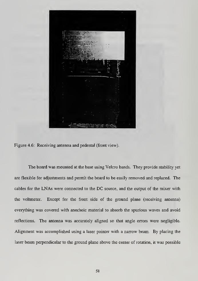
Figure 4.6: Receiving antenna and pedestal (front view).

The board was mounted at the base using Velcro bands. They provide stability yet

are flexible for adjustments and permit the board to be easily removed and replaced. The

cables for the LNAs were connected to the DC source, and the output of the mixer with

the voltmeter. Except for the front side of the ground plane (receiving antenna)

everything was covered with anechoic material to absorb the spurious waves and avoid

reflections. The antenna was accurately aligned so that angle errors were negligible.

Alignment was accomplished using a laser pointer with a narrow beam. By placing the

laser beam perpendicular to the ground plane above the center of rotation, it was possible

58

to place the laser beam on the transmit horn thereby aligning the test antenna to the

emitter.

Located in the adjacent instrumentation room are the voltmeter, the voltage source

which provides the 15 Volts DC to the LNAs, the HP8510 network analyzer, and the

computer controller. The latter is used to control the transmitter signal and the rotation of

the pedestal. It was programmed to sample the voltmeter and record the measured DC

values out of the mixer at specified angles. The data were taken manually by two people.

The first person called out the angle and the second recorded the DC voltage at that

instant. The measurements were taken every 0.5 degrees from - 90 to 90 degrees. For

each channel the measurements were taken several times so that any measurement errors

could be uncovered. However, all data repeated without any significant deviations.

B. MEASURED ARRAY RESPONSE DATA

The measurements on the first channel were taken and the ideal response vs

measured response is shown in Figure 4.7. The gray line presents the ideal and the black

the measured data. The differences are very small for angles between -60 and 60 degrees.

Outside this region the errors are larger due to the reflection and scattering from the edges

of the ground plane which are illuminated by the source at these angles. Another source

of difference is the element patterns of the open-ended waveguides. Near cpB= 0° the

element patterns vary little but towards ± 90° mutual coupling differences are significant

due to the nonperiodic spacing of the elements.

59

300

200

100

^_^>E<DO)£ -100o>

-200

300

I

—

1

1 1 .1 1 1 1

lllllill ft\

J III

1 I

1 1 1 1

1111111/ ;

_i 1 1 i i

40 -20 20 40Angle of arrival (degrees)

60 80

Figure 4.7: Plot of ideal vs measured data for d = 75X

.

The measurements of voltage mixer output versus angle of incidence as they were

taken from the computer and the voltmeter are presented in Appendix C (Tables C.l to

C4).

Response data was measured for the second channel whose baseline was 0.6

wavelengths. The construction procedure was similar to that for the first channel. As

mentioned, since we had only four LNAs, the first channel had to be disassembled in

order to construct the second. The measurements were taken using the same procedure as

described for the first channel. Figure 4.8 shows the ideal (gray curve) and the measured

60

data (black curve) for the voltage at the mixer output versus angle of incidence. Within

the area of interest (-60 to 60 degrees) the only deviation observed is a phase shift (i.e.,

translation of the curve along the horizontal axis). For this signal to be of use in the SNS

logic block, the voltage must have its minimum value at -90 degrees. Although the

channel was designed to add the appropriate y/ an unwanted phase shift occurred during

assembly, leading to a shifted curve. Additional phase trimming can eliminate this

mismatch. Tables C.5 to C.8 in Appendix C present the measurements of voltage mixer

output versus angle of incidence as they were taken from the computer and the voltmeter.

80 -60 -40 -20 20 40Angle of arrival (degrees)

300

—11 1

1 1 1 11

^x\ ftfli in \ 1 1 1 1 i\ /200 v\ llliv 1 1 1\ /

Si 1 i100

• III 1 II

1

i i/i>E

enCO

Q-100

>i

-2001

1

1

/ /

-300 Ww urn iii i i i

'fill 1 v .

-i i i i i L

60 80

Figure 4.8: Plot of ideal vs measured data ford = 6X .

61

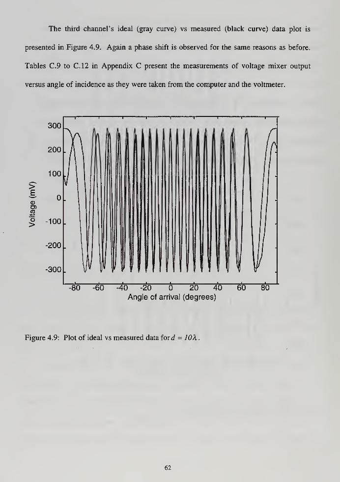
The third channel's ideal (gray curve) vs measured (black curve) data plot is

presented in Figure 4.9. Again a phase shift is observed for the same reasons as before.

Tables C.9 to C.12 in Appendix C present the measurements of voltage mixer output

versus angle of incidence as they were taken from the computer and the voltmeter.

>E.

<DO)CO

o>

-80 -60 -40 -20 20 40Angle of arrival (degrees)

300i i i i i

illinium

T 1 1 1

lillilt L200

Ai illf

100

1 1 /

1001 I-

•200 I

1

1

III/-300 ; P lllllllllll lllllliF

.

j i i i 1

60 80

Figure 4.9: Plot of ideal vs measured data ford = 10X

62

V. CONCLUSIONS

This thesis discussed the design and construction of a direction finder which uses

the phase comparison method to determine the direction of the emitter. The frequency of

interest is 8.5 GHz and the processing of the signal is performed with a logic block whose

operation is based on the symmetrical number system. Four antenna elements are used

forming three pairs, with one element common for all the pairs. The output of the two

elements of each pair are mixed together, and the DC voltage at the output is fed the logic

block. In the course of this research all the components were tested and the arrays

assembled and measured in the anechoic chamber to verify that their operation was as

expected from theory.

The use of an already fabricated and available ground plane for an array based on

a residue number system limited the angular range of unambiguous angle estimates

compared to the larger range that would exist had the array been designed for SNS

processing. Also the lack of some hardware components such as LNAs restricted the

scope of the research: only one channel could be constructed and tested at a time. Thus it

was not possible to test the whole array and beamforming network in the anechoic

chamber.

The measured results were in agreement with theory. The curves had the same

number of cycles as predicted by the equations, but were phase shifted (translated)

because of phase deviations unintentionally introduced in the assembly process. For the

curves to be usable for the SNS logic block, they must have a minimum voltage value at

- 90 degrees, which was not true for two arrays due to the unintended phase shifts. A

63

further phase trimming on the assembled antenna can easily eliminate the unwanted phase

differences. The SNS direction finding array has great promise for providing accurate,

unambiguous DOA estimates and this research has provided a proof of concept.

The next step should be the assembly of the entire array and beamforming

network. To accomplish this more amplifiers must be purchased. The three channels can

then be tested as a direction finding array by connecting the DC output to the SNS AID

converter.

After the array performance has been demonstrated a new aperture should be

constructed with the proper SNS element spacings, which are 3, 3.75, and 5 wavelengths

respectively. Using these distances between elements unambiguous DOA estimates can

be obtained.

Future studies should also examine the quantization error characteristics and the

frequency correction schemes proposed in [Ref 5].

64

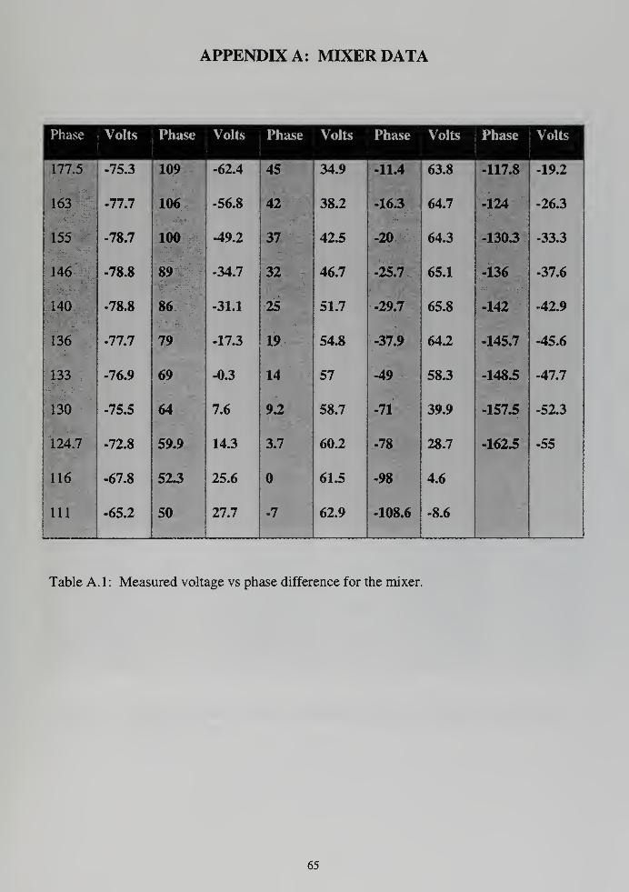
APPENDIX A: MIXER DATA

Phase Volts Phase Volts Phase Volts Phase Volts Phase Volts

177.5 -75.3 109 -62.4 45 34.9 -11.4 63.8 -117.8 -19.2

163 -77.7 106 -56.8 42 38.2 -16.3 64.7 -124 -26.3

155 -78.7 100 -49.2 37 42.5 -20 64.3 -1303 -333

146 -78.8 89 -34.7 32 46.7 -25.7 65.1 -136 -37.6

140 -78.8 86 -31.1 25 51.7 -29.7 65.8 -142 -42.9

136 -77.7 79 -17.3 19 54.8 -37.9 64.2 -145.7 -45.6

133 -76.9 69 -03 14 57 -49 58.3 -148.5 -47.7

130 -75.5 64 7.6 9.2 58.7 -71 39.9 -157.5 -52.3

124.7 -72.8 59.9 14.3 3.7 60.2 -78 28.7 -162^ -55

116 -67.8 523 25.6 61.5 -98 4.6

111 -65.2 50 27.7 -7 62.9 -108.6 -8.6

Table A. 1 : Measured voltage vs phase difference for the mixer.

65

66

APPENDIX B: LNA DATA

Input Power Output Input Power Output Input Power Output

Power Power Power

-59.4 -13.28 -45.32 0.16 -31.49 8.97

-58.2 -12.17 -44.33 1.07 -30.41 9.17

-57.8 -11.82 -43.32 2.05 -29.29 9.34

-56.8 -10.82 -42.28 2.97 -28.17 9.48

-55.8 -9.93 -41.22 3.89 -27.25 9.58

-54.78 -8.92 -40.14 4.77 -26.32 9.64

-53.7 -7.92 -39.05 5.62 -25.37 9.69

-52.6 -6.9 -37.99 6.38 -24.39 9.73

-51.55 -5.84 -37.47 6.7 -23.39 9.75

-50.45 -4.77 -36.53 7.27 -22.35 9.75

-49.31 -3.66 -35.56 7.72 -21.27 9.75

-48.16 -2.56 -34.58 8.09 -20.19 9.74

-47.24 -1.64 -33.57 8.43 -19.09 9.74

-46.29 -0.74 -32.54 8.74

Table B. 1 : Input power measurements vs output power for LNA 450873. For the real

input power values add 10 dB.

67

Input Power Output Input Output Input Output

Power Power Power Power Power

-59.5 -13.89 -45.33 -0.49 -31.7 8.09

-58.4 -12.77 -44.33 0.46 -30.6 8.28

-58 -12.44 -43.38 1.34 -29.46 8.44

-56.91 -11.5 -42.33 2.3 -28.32 8.55

-55.89 -10.55 -41.26 3.24 -27.41 8.64

-54.8 -9.55 -40.18 4.15 -26.48 8.71

-53.74 -8.56 -39.06 5.02 -25.56 8.7

-52.65 -7.52 -37.93 5.78 -2436 8.74

-51.56 -6.47 -37.43 6.08 -23.55 8.76

-50.47 -5.42 -36.49 6.56 -22.51 8.76

-49.32 -4.31 -35.53 6.97 -21.42 8.75

-48.17 -3.21 -34.54 7.33 -20.33 8.74

-47.27 -2.34 -33.54 7.65 -19.23 8.72

-46.3 -1.42 -32.51 7.94

Table B.2: Input power measurements vs output power for LNA 450874. For the real

input power values add 10 dB.

68

Input Output Input Output Input Output

Power Power Power Power Power Power

-59.79 -12.76 -45.45 0.58 -31.67 8.24

-58.43 -11.63 -44.49 1.47 -30.59 8.36

-58.04 -11.29 -43.47 2.4 -29.47 8.45

-57.01 -10.36 -42.42 3.33 -28.35 8.52

-55.98 -9.42 -41.36 4.24 -27.44 8.57

-54.91 -8.45 -40.42 4.99 -26.51 8.59

-53.84 -7.44 -39.28 5.77 -25.56 8.6

-52.76 -6.41 -38.15 6.4 -24.59 8.61

-51.66 -5.35 -37.64 6.63 -23.58 8.6

-50.54 -4.28 -36.7 7.01 -22.54 8.59

-49.4 -3.18 -35.73 7.35 -21.46 8.59

-48.25 -2.08 -34,75 7.64 -20.37 8.59

-47.34 -1.21 -33.75 7.9 -19.26 8.61

-46.39 -0.3 -32.72 8.09

Table B.3: Input power measurements vs output power for LNA 450875. For the real

input power values add 10 dB.

69

Input Output Input Output Input Output

Power Power Power Power Power Power

-59.3 -12.52 -45.39 0.4 -31.47 7.81

-58.16 -11.42 -44.38 1.55 -30.39 7.91

-57.78 -11.1 -43.36 2.44 -29.28 8

-56.74 -10.19 -42.32 3.32 -28.15 8.06

-55.72 -9.26 -41.26 4.15 -27.24 8.1

-54.68 -8.33 -40.17 4.89 -26.31 8.11

-53.62 -7.34 -39.06 5.53 -25.35 8.11

-52.54 -6.33 -37.96 6.09 -24.38 8.1

-51.46 -5.31 -37.45 6.29 -23.38 8.08

-50.35 -4.25 -36.5 6.65 -22.34 8.06

-49.2 -3.15 -35.53 6.98 -21.25 8.05

-48.05 -2.07 -34.55 7.26 -20.17 8.06

-47.35 -1.25 -33.55 7.5 -19.08 8.07

-46.38 -0.38 -32.52 7.68

:

-> V* ':r^

Table B.4: Input power measurements vs output power for LNA 451376. For the real

input power values add 10 dB.

70

APPENDIX C: MEASURED ARRAY RESPONSE DATA

Angle Volts Angle Volts Angle Volts Angle Volts Angle Volts

-90 250 -80 289.4 -70 -117 -60 226 -50 -160

-89.5 255 -79.5 289.4 -69.5 -180 -59.5 257 -49.5 -74

-89 258 -79 289.3 -69 -220 -59 280 -49 33

-88.5 262 -78.5 289.1 -68.5 -254 -583 287 -48.5 129

-88 265 -78 288.7 -68 -274 -58 293 -48 207

-87.5 268 -77.5 287.9 -67.5 -288 -85.5 284 -47.5 257

-87 271 -77 286.4 -67 -296 -57 259 -47 285

-86.5 275 -76.5 284.2 -66.5 -298 -56.5 220 -46.5 294

-86 278 -76 280 -66 -294 -56 170 -46 285

-85.5 279 -75.5 274 -65.5 -293 -55.5 99 -45.5 260

-85 284 -75 273 -65 -272 -55 28 -45 215

-84.5 286 -74.5 255 -64.5 -253 -543 -75 -44.5 154

-84 289 -74 240 -64 -220 -54 -159 -44 67

-83.5 288 -73.5 215 -63.5 -204 -53.5 -230 -43.5 -36

-83 290 -73 190 -63 -140 -53 -265 -43 -155

-82.5 290 -72.5 155 -62.5 -85 -52.5 -290 -42.5 -229

-82 290 -72 110 -62 -28 -52 -298 -42 -278

-81.5 289 -71.5 65 -61.5 51 -51.5 -292 -41.5 -296

-81 289.4 -71 47 -61 120 -51 -266 -41 -297

-80.5 289.3 -70.5 -60 -60.5 75 -50.5 -225 -405 -275

Table C. 1 : Voltage at mixer output vs DOA measurements for d = 7.5X (-90 to -39.5

deg).

71

Angle Volts Angle Volts Angle Volts Angle Volts

-40 -232 -30 -21 -20 288 -10 58

-39.5 -148 -29.5 110 -19.5 290 -95 -158

-39 -46 -29 215 -19 257 -9 -250

-38.5 95 -28.5 272 -185 191 -8.5 -289

-38 193 -28 289 -18 85 -8 -298

-37.5 258 -275 286 -175 -50 -75 -270

-37 287 -27 250 -17 -186 -7 -202

-36.5 292 -265 181 -165 -267 -65 -84

-36 270 -26 87 -16 -296 -6 75

-35.5 223 -255 -43 -155 -292 -55 200

-35 151 -25 -178 -15 -253 -5 271

-34.5 56 -245 -257 -145 -171 -45 293

-34 -81 -24 -289 -14 -33 -4 288

-33.5 -189 -235 -298 -135 108 -35 230

-33 -263 -23 -277 -13 226 -3 145

-32.5 -290 -225 -219 -125 277 -25 20

-32 -298 -22 -115 -12 294 -2 -135

-31.5 -277 -215 30 -115 272 -15 -244

-31 -228 -21 167 -11 217 -1 -287

-30.5 -145 -205 253 -105 121 -05 -297

Table C.2: Voltage at mixer output vs DOA measurements for d = 75X (-40 to 0.5 deg).

72

Angle Volts Angle Volts Angle Volts Angle Volts

-297.8 10 249 20 262 30 -168

0.5 -209 10.5 289 20.5 50 303 -245

1 -94 11 289.5 21 -70 31 -283

1.5 60 11.5 259 21.5 -203 313 -298

2 192 12 186 22 -263 32 -288

2.5 260 12.5 85 223 -293 323 -257

3 293 13 -60 23 -296 33 -191

3.5 282 13.5 -188 23.5 -270 333 -82

4 236 14 -268 24 -210 34 39

4.5 147 14.5 -295 24.5 -121 343 159

5 34 15 -293 25 -18 35 231

5.5 -127 15.5 -263 25.5 142 353 278

6 -226 16 -187 26 228 36 293

6.5 -282 16.5 -66 26.5 274 36.5 285

7 -298 17 77 27 293 37 260

7.5 -280 17.5 200 273 284 373 200

8 -236 18 272 28 248 38 121

8.5 -123 18.5 293 28.5 182 383 30

9 38 19 283 29 76 39 -97

9.5 60 19.5 234 29.5 -30 39.5 -197

Table C.3: Voltage at mixer output vs DOA measurements for d = 7_5A(0 to 39.5 deg).

73

Angle Volts Angle Volts Angle Volts Angle Volts Angle Volts

40 -257 50 1 60 291 70 -293 80 13.2

40.5 -285 50.5 -93 605 294 70.5 -285 805 42

41 -298 51 -179 61 290 71 -275 81 66 1

!

41.5 -293 51.5 -238 61.5 281 71.5 -264 815 92i

42 -272 52 -270 62 266 72 -250 82

i

111

2.5 -235 52.5 -292 62.5 246 72.5 -236 825 133

43 -172 53 -298 63 217 73 -222 83 147

43.5 -85 53.5 -291 63.5 184 73.5 -207 83.5 156

44 9 54 -271 64 146 74 -194 84 161

44.5 108 54.5 -241 64.5 95 74.5 -182 845 162

45 186 55 -200 65 40 75 -170 85 162

45.5 238 553 -140 65.5 -27.8 755 -158 85.5 1635

46 273 56 -65 66 -96 76 -147 86 167.7

46.5 290 56.5 5 66.5 -172 765 -134 865 175

47 292 57 87 67 -221 77 -118 87 188i

47.5 282 57.5 151 67.5 -257 775 -101 875 192

48 253 58 203 68 -279 78 -80 88 219

84.5 211 58.5 239 68.5 -291 78.5 -57 885 233

49 156 59 266 69 -297 79 -35 89 240

49.5 83 59.5 282 69.5 -297.5 795 -10 895i

251

Table C.4: Voltage at mixer output vs DOA measurements for d = 7.5A (40 to 89.5 deg).

74

Angle Volts Angle Volts Angle Volts Angle Volts Angle Volts

-90 239 -80 230 -70 239 -60 -286 -50 140

-89.5 240 -79.5 237 -693 213 -593 -277 -49.5 84

-89 239 -79 243 -69 187 -59 -263 -49 6

-88.5 238 -78.5 248 -68.5 151 -583 -245 -483 -79

-88 233 -78 253 -68 118 -58 -215 -48 -153

-87.5 229 -77.5 259 -67.5 108 -853 -169 -473 -217

-87 222 -77 263 -67 67 -57 -108 -47 -254

-86.5 234 -76.5 266 -663 -39 -563 -14 -463 -275

-86 205 -76 269 -66 -90 -56 63 -46 -288

-85.5 200 -75.5 273 -65.5 -140 -553 144 -45.5 -294

-85 193 -75 275 -65 -184 -55 198 -45 -290

-84.5 190.8 -74.5 277 -64.5 -213 -54.5 244 -443 -280

-84 190.8 -74 279 -64 -238 -54 265 -44 -257

-83.5 192 -73.5 280 -63.5 -256 -533 277 -433 -222

-83 196 -73 279 -63 -269 -53 281 -43 -165

-82.5i

199 -72.5 277 -62.5 -279 -52.5 277 -42.5 -71

-82 206 -72 274 -62 -287 -52 264 -42 36

-81.5 212 -71.5 267 -61.5 -292 -513 248 -413 137

i

-si 218 -71 260 -61 -293 -51 222 -41 200

|-80.5 224 -703 247 -60.5 -291 -50.5 187 -403 249

Table C.5: Voltage at mixer output vs DOA measurements for d = 6X (-90 to -39.5deg).

75

Angle Volts Angle Volts Angle Volts Angle Volts

-40 270 -30 122 -20 -55 -10 71

-39.5 281 -29.5 205 -195 134 -95 195

-39 280 -29 253 -19 216 -9 244

-38.5 266 -28.5 274 -18.5 262 -85 275

-38 241 -28 282 -18 279 -8 282

-37.5 206 -27.5 275 -175 281 -75 270

-37 147 -27 256 -17 265 -7 241

-36.5 70 -26.5 222 -165 233 -65 192

-36 -31 -26 174 -16 178 -6 104

-35.5 -125 -25.5 90 -155 102 -55 -3

-35 -211 -25 -5 -15 -15 -5 -132

-34.5 -257 -24.5 -123 -145 -142 -45 -220

-34 -282 -24 -213 -14 -232 -4 -272

-33.5 -293 -235 -265 -135 -273 -35 -292

-33 -291 -23 -288 -13 -292 -3 -292.8

-32.5 -276 -225 -294 -125 -292.8 -25 -275

-32 -250 -22 -285 -12 -277 -2 -245

-31.5 -202 -215 -260 -11.5 -240 -15 -172

-31 -109 -21 -214 -11 -179 -1 -50

-30.5 18 -205 -130 -105 -53 -05 96

Table C.6: Voltage at mixer output vs DOA measurements for d =6X (-40 to 0.5 deg).

76

Angle Volts Angle Volts Angle Volts Angle Volts

197 10 258 20 270 30 246

0.5 250 10.5 277 205 282 305 271

1 277 11 281 21 276 31 282

1.5 282 115 270 215 251 315 278

2 268 12 235 22 208 32 261

2.5 237 12.5 183 225 140 325 231

3 179 13 100 23 44 33 187

3.5 93 13.5 -15 235 -76 335 116

4- V -15 14 -143 24 -179 34 31

4.5 -153 14.5 -230 245 -243 34.5 -76

5 -233 15 -270 25 -277 35 -167

5.5 -276 15.5 -291 255 -292 35.5 -239

6 -292 16 -293 26 -294 36 -270

6.5 -291 16.5 -277 265 -281 365 -289

7 -271 17 -247 27 -256 37 -295

7.5 -230 17.5 -181 275 -211 375 -286

8 -146 18 -65 28 -127 38 -267

8.5 10 185 73 285 -7 385 -235

9 124 19 177 29 115 39 -176

9.5 207 195 242 295 195 39.5 -91

Table C.7: : Voltage at mixer output vs DOA measurements for d = 6X (0 to 39.5 deg).

77

Angle Volts Angle Volts Angle Volts Angle Volts Angle Volts

40 17 50 -294 60 260 70 -294.2 80 -140

40.5

41

111

191

505

51

-292

-284

60.5

61

248

231

705

71

-292

-289

805

81

-118

-100

41.5 238 51.5 -267 615 214 71.5 -285 815 -75

42 262 52 -242 62 194 72 -281 82 -52

2.5 277 525 -210 625 170 725 -277 825 -31

43 282 53 -160 63 145 73 -273 83 -9.9

43.5 278 535 -90 635 114 735 -268 835 5.7

44 266 54 -11.5 64 78 74 -263 84 17.7

44.5 246 54.5 56 645 34 745 -258 84.5 22.6

45 219 55 125 65 -9 75 -252 85 2.9

45.5 187 55.5 177 655 -68 755 -246 85.5 20.3

46 128 56 216 66 -125 76 -238 86 18.4

46.5 62 565 243 66.5 -185 76.5 -230 86.5 29

47 -19 57 264 67 -227 77 -220 87 59

47.5 -110 575 275 675 -255 775 -210 875 98

48 -188 58 281 68 -273 78 -200 88 126

84.5 -239 585 282 685 -285 785 -186 88.5 142

49 -266 59 278 69 -291 79 -172 89 148

49.5 -285 595 270 695 -294 795 -156 89.5 150

Table C.8: Voltage at mixer output vs DOA measurements for d = 6X (40 to 89.5 deg).

78

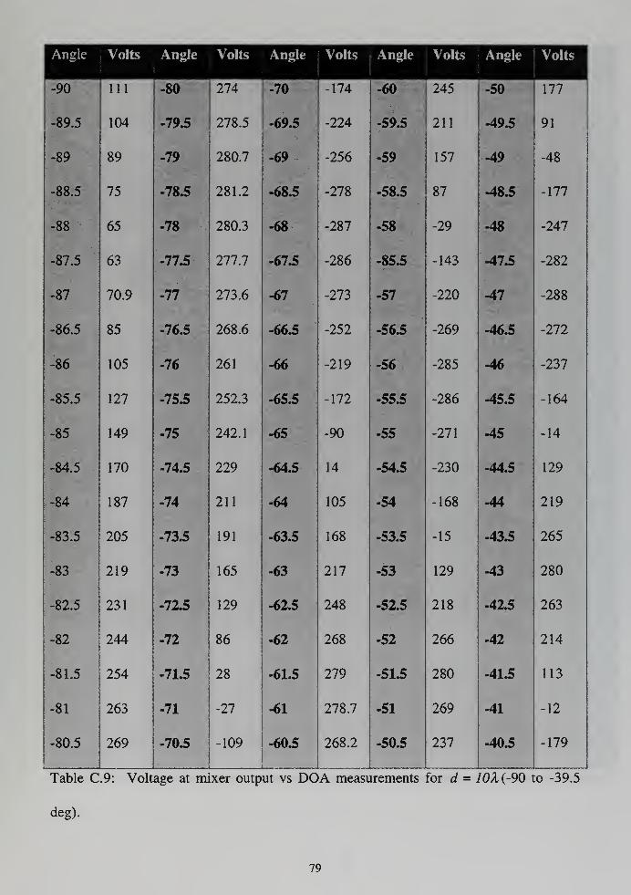
Angle Volts Angle Volts Angle Volts Angle Volts Angle Volts

-90 111 -80 274 -70 -174 -60 245 -50 177

-89.5 104 -79,5 278.5 -69.5 -224 -59.5 211 -49.5 91

-89 89 -79 280.7 -69 -256 -59 157 -49 -48

-88.5 75 -78.5 281.2 -68.5 -278 -58.5 87 -48.5 -177

-88 65 -78 280.3 -68 -287 -58 -29 -48 -247

-87.5 63 -77.5 277.7 -67.5 -286 -85.5 -143 -47.5 -282

-87 70.9 -77 273.6 -67 -273 -57 -220 -47 -288

-86.5 85 -76.5 268.6 -66.5 -252 -56.5 -269 -46.5 -272

-86 105 -76 261 -66 -219 -56 -285 -46 -237

-85.5 127 -75.5 252.3 -65.5 -172 -55.5 -286 -45.5 -164

-85 149 -75 242.1 -65 -90 -55 -271 -45 -14

-84.5 170 -74.5 229 -64.5 14 -54.5 -230 -44.5 129

-84 187 -74 211 -64 105 -54 -168 -44 219

-83.5 205 -73.5 191 -63.5 168 -53.5 -15 -43.5 265

-83 219 -73 165 -63 217 -53 129 -43 280

|

-82.5 231 -7Z5 129 -62.5 248 -52.5 218 -42.5 263

J

-82 244 -72 86 -62 268 -52 266 -42 214

-81.5 254 -71.5 28 -61.5 279 -51.5 280 -41.5 113

-81 263 -71 -27 -61 278.7 -51 269 -41 -12

-80.5 269 -70.5 -109 -60.5 268.2 -50.5 237 -40.5 -179

Table C.9: Voltage at mixer output vs DOA measurements for d = 10X(-90 to -39.5

deg).

79

Angle Volts Angle Volts Angle Volts Angle Volts

-40 -258 -30 233 -20 -289 -10 7

-39.5 -289 -29.5 275 -19.5 -271 -95 -125

-39 -282 -29 273 -19 -211 -9 -244

-38.5 -241 -28.5 233 -18.5 -38 -85 -287

-38 -150 -28 142 -18 175 -8 -273

-37.5 38 -27.5 40 -17.5 256 -75 -212

-37 187 -27 -204 -17 281 -7 -30

-36.5 256 -26.5 -275 -16.5 252 •6S 156

-36 280 -26 -289 -16 161 -6 258

-35.5 215 -25.5 -261 -155 5 -55 282

-35 115 -25 -197 -15 -200 -5 252

-34.5 60 -24.5 -15 -14.5 -274 -4.5 170

-34 -60 -24 160 -14 -285 -4 -29

-33.5 -199 -235 255 -135 -253 -35 -214

-33 -274 -23 280 -13 -144 -3 -278

-32.5 -288 -225 262 -125 85 -25 -280

-32 -266 -22 182 -12 213 -2 -230

-31.5 -211 -215 36 -11.5 276 -15 -101

-31 -47 -21 -157 -11 273 -1 120

-30.5

:

:

139 -205 -256 -105 210 -05 242

Table CIO: Voltage at mixer output vs DOA measurements for d = 10X (-40 to 0.5 deg).

80

Angle Volts Angle Volts Angle Volts Angle Volts

280 10 -81 20 -274 30 261

0.5 266 10.5 135 20.5 -261 303 201

1 197 11 251 21 -177 31 91

1.5 53 11.5 281 21.5 -9 313 -107

2 -169 12 261 22 175 32 -234

2.5 -263 12.5 177 22.5 263 323 -280

3 -287 13 16 23 282 33 -284

3.5 -260 13.5 -172 233 254 333 -256

4 -182 14 -270 24 182 34 -188

4.5 31 14.5 -287 24.5 42 34.5 -54

5 193 15 -261 25 -137 35 140

5.5 270 15.5 -184 25.5 -247 35.5 227

6 281 16 19 26 -285 36 273

6.5 237 163 191 263 -278 363 281

7 140 17 264 27 -236 37 248

7.5 -57 17.5 281 273 -133 373 181

8 -224 18 240 28 65 38 68

8.5 -284 183 140 283 202 383 -95

9 -276 19 -13 29 263 39 -194

9.5 -228

i

19.5 -207 29.5 282 393 -272

Table C.ll: : Voltage at mixer output vs DOA measurements for d = 102.(0 to 39.5

deg).

81

Angle Volts Angle Volts Angle Volts Angle Volts Angle Volts

40 -287 50 52 60 -184 70 -215 80 -102

40.5 -240 505 166 605 -125 705 -243 80.5 -72

41 -166 51 235 61 -32 71 -261 81 -38

41.5 -6 51.5 268 615 66 715 -283 815 -3

42 141 52 282 62 141 72 -284 82 43

2.5 225 525 271 625 193 725 -285 825 83

43 267 53 243 63 235 73 -284 83 118

43.5 282 535 194 635 261 735 -282 835 145

44 270 54 147 64 276 74 -278 84 172

44.5 239 545 15 645 282 745 -272 84.5 202

45 176 55 -80 65 275 75 -266 85 215

45.5 82 55.5 -188 655 259 755 -258 85.5 225\

46 -58 56 -243 66 232 76 -250 86

i

233

46.5 -171 565 -271 66.5 192 765 -241 865 239

47 -249 57 -284 67 142 77 -230 87 242.5

47.5 -286 57.5 -286 675 84 775 -212 875 242.5

48 -275 58 -279 68 20 78 -187 88 240.5

84.5 -247 58.5 -267 685 -56 785 -165 88.5 236

49 -192 59 -248 69 -122 79 -147 89 228

49.5 -111 59.5 -220 69.5 -178 79.5 -124 89.5 216

Table C 12: Voll age at mixer outpiit vs DO^, measure:ments foi• d = 10/L (40 to 89>.5 deg)

82

LIST OF REFERENCES

1. Herndon H. Jenkins, Small-Aperture Radio Direction Finding, Artech House Inc,

Norwood, MA, 1991.

2. Byron Edde, Radar Principles, Technology, Applications, Prentice-Hall, Inc, Upper

Saddle Ricer, NJ, 1993.

3. Matthew Sadiku, Elements of Electromagnetics, Saunders College Publishing,

Orlando, FL, 1994.

4. Luis E. Moita Rodrigues, "High-Resolution Residue Antenna Architectures for

Wideband Direction Finding," Naval Postgraduate School Master's Thesis, June

1996.

5. Byeong-Jun Park, "Interpolation Techniques in High-Resolution Residue Antenna

Architectures," Naval Postgraduate School Master's Thesis, September 1996.

6. P. E. Pace, J. L. Schafer, D. Styer, "Optimum Analog Preprocessing for Folding

ADCs," IEEE Transactions on Circuits and Systems-II Analog and Digital Signal

Processing, Vol. 42, No 12, pp 825-829, December 1989.

83

84

INITIAL DISTRIBUTION LIST

No of Copies

1. Defence Technical Information Center 2

8725 John J. Kingman Rd., STE 0944

Ft. Belvoir, VA 22060-6218

2. Dudley Knox Library, Code 52 2

Naval Postgraduate School

411 Dyer Rd.

Monterey, Ca 93943-5101

3. Chairman, Code EC 1

Department of Electrical and Computer Enginering

Naval Postgraduate School

Monterey, CA, 93943-5121

4. Professor Phillip E. Pace, Code EC/PC 4

Department of Electrical and Computer Engineering

Naval Postgraduate School

Monterey, CA, 93943-5121

5. Professor David C. Jenn, Code EC/JN 2

Department of Electrical and Computer Engineering

Naval Postgraduate School

Monterey, CA, 93943-5121

6. Bob Vitale, Code EC/ELDepartment of Electrical and Computer Engineering 1

Naval Postgraduate School

Monterey, CA, 93943-5121

7. Lt Panayiotis Papandreou 2

Kononos 31, Pagrati,

Athens, 11634, GREECE

8. Cmdr Ioannis Papandreou 1

Kononos 31, Pagrati,

Athens, 11634, GREECE

85

G483NPGTH

10/99 22527-200 nule

2765I