Design and Performance Calculations of a Propeller for Very High Altitude Flight

L

NASA / TM--1998-20663 7

Design and Performance Calculations of a

Propeller for Very High Altitude Flight

L. Danielle Koch

Lewis Research Center, Cleveland, Ohio

National Aeronautics and

Space Administration

Lewis Research Center

February 1998

::ii!ili!i_....

:iii!iiiiii_._

NASA Center for Aerospace Information

800 Elkridge Landing Road'Lin_icum Heights, MD 21090-2934.Price Code: A07

Available from.

National Technical Information Service

5287 Port Royal Road

Springfield, VA 221!2_)Price Code: A07

DESIGN AND PERFORMANCE CALCULATIONS OF A PROPELLER

FOR VERY HIGH ALTITUDE FLIGHT

by

L. DANIELLE KOCH

Submitted in partial fulfillment of the requirements

for the degree of Masters of Science in Engineering

Thesis Advisor: Dr. Eli Reshotko

Department of Mechanical and Aerospace Engineering

CASE WESTERN RESERVE UNIVERSITY

DESIGN AND PERFORMANCE CALCULATIONS OF A PROPELLER

FOR VERH HIGH ALTITUDE FLIGHT

:,ii!_:_iiii!il

'iiiii_

by

L. DANIELLE KOCH

ABSTRACT

Reported here is a design study of a propeller for a vehicle capable of subsonic

flight in Earth's stratosphere. All propellers presented were required to absorb 63.4

kW (85 hp) at 25.9 km (85,000 r) while aircraft cruise velocity was maintained at

Mach 0.40. To produce the final design, classic momentum and blade-element

theories were combined with two and three-dimensional results from the Advanced

Ducted Propfan Analysis Code (ADPAC), a numerical Navier-Stokes analysis code.

The Eppler 387 airfoil was used for each of the constant section propeller

designs compared. Experimental data from the Langley Low-Turbulence Pressure

Tunnel was used in the strip theory design and analysis programs written. The

experimental data was also used to validate ADPAC at a Reynolds numbers of 60,000

and a Mach number of 0.20. Experimental and calculated surface pressure

coefficients are compared for a range of angles of attack.

Since low Reynolds number transonic experimental data was unavailable,

ADPAC was used to generate two-dimensional section performance predictions for

Reynolds numbers of 60,000 and 100,000 and Mach numbers ranging from 0.45 to

vii

0.75. Surfacepressurecoefficientsarepresentedfor selectedanglesof attack, in

additionto thevariationof lift and drag coefficients at each flow condition.

A three-dimensional model of the final design was made which ADPAC used

to calculated propeller performance. ADPAC performance predictions were _iiiiii!

compared with strip-theory calculations at design point. Propeller efficiency

predicted by ADPAC was within 1.5% of that calculated by strip theory methods,

although ADPAC predictions of thrust, power, and torque coefficients were

approximately 5% lower than the strip theory results. Simplifying assumptions made

in the strip theory account for the differences seen.

iiiil

viii

ACKNOWLEDGEMENTS

!ii:_:

How fortunate I am to have so many blessings to count! For their patience

and guidance, I would like to thank Dr. Eli Reshotko and Dr. Christopher Miller. It

takes special skill to be a teacher, and I am sincerely grateful to have been able to

learn by your examples.

For their unfailing enthusiasm, I would like to thank Dave Bents and Tony

Colozza.of the ERAST team. It has been a long and bumpy road, and your optimism

has really made a difference.

For making financial support available, I would like to thank NASA, Jeff

Haas, Wayne Thomas, and Chuck Mehalie. While slightly beyond the boundaries of

my normal assigned duties, I believe that I am a better engineer because of the

experience gained through this thesis work.

ix

CONTENTS

ABSTRACT ................................................................................................................. vii

ACKNOWLEDGEMEI_S .......................................................................................... ix

NOMENCLATURE ...................................................................................................... xi

CHAPTER 1--Introduction ........................................................................................... 1

CHAPTER 2---Selection of Airfoil and Airfoil Performance Data .............................. 6

CHAPTER 3---Grid Study and ADPAC Validataion .................................................. 22

CHAPTER 4---Propeller Design Using Experimental Airfoil Data .......................... 42

CHAPTER 5---ADPAC Two-Dimensional Aerodynamic Predictions .................... 52

CHAPTER 6---Propeller Design and Analysis UsingTwo-Dimensional ADPAC Predictions ............................................ 86

CHAPTER 7---ADPAC Three-Dimensional Performance Calculations ................... 97

CHAPTER 8--Conclusion ....................................................................................... 114

REFERENCES ........................................................................................................ 116

NOMENCLATURE

....ii!!!!_'_ii!iiii!!i:i

a = speed of sound

C

Cd =

CI =

Cp

chord

drag coefficient = D/(qS)

lift coefficient = L/(qS)

pressure coefficient= ( )2 ,, 2+(r-OM (y)M,o 2 2 +(y -1)M _

CP =

CQ

CT =

power coefficient = P/(pn3d s)

torque coefficient = Q/(pn2d s)

thrust coefficient = T/(pn2d 4)

d = diameter

D = drag

e specific stored energy

advance ratio = V/(nd)

L = lift

M = Mach number = V/a

n = rotational speed

P = power

q ._. dynamic pressure = 0.5pV 2

Q = torque

xi

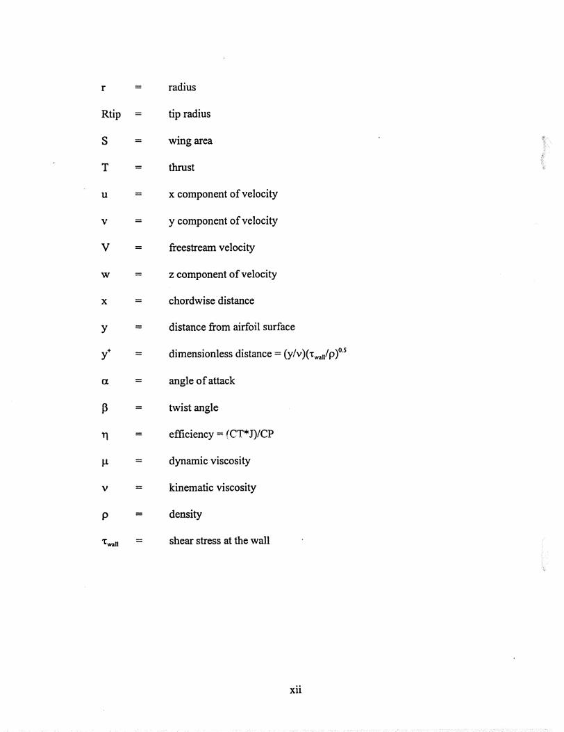
r = radius

Rtip = tip radius

T

= wing area

= thrust

ii!ili!!i_'

U x component of velocity

V y component of velocity

V freestream velocity

W z component of velocity

x = chordwise distance

ydistance from airfoil surface

dimensionless distance = (y/v)(XwJ9) °s

t_ = angle of attack

13 = twist angle

efficiency = (CT*J)/CP

dynamic viscosity

V kinematic viscosity

p = density

"l_wail = shear stress at the wallii,_i!_ i

xii

CHAPTER 1-INTRODUCTION

Background

Concern for the environment and determination to overcome a new challenge

can make very high altitude subsonic flight possible. Driven by the needs of the

atmospheric research community, a remotely piloted vehicle capable of flying

subsonically in the stratosphere is being developed by a consortium of federal,

industrial, and academic partners under NASA's Environmental Research Aircraft

and Sensor Technology (ERAST) program.

In-situ measurements at altitudes between 24.4 km (80,000 fi)and 30.5 km

(100,000 ft) are needed to further our understanding of the dynamics and chemistry

of Earth's atmosphere. These measurements would augment laboratory research, data

from samples of the lower stratosphere taken by the ER-2 aircraft, and measurements

from satellites and balloons. A better fundamental understanding of the atmosphere

can help us to make more responsible decisions in the way we choose to live, ,,v_._,rk_

and travel.

Undeniably, development of a suitable propulsion system is the most

formidable challenge. Currently, there are no existing propulsion systems capable of

meeting either the program's near term altitude goal of 25.3 km (83,000 ft) or

ultimate goal of 30.5 km (100,000 ft). Studies summarized by the ERAST program's

Leadership Team ( Ref. 1) suggest that the near term goal may be met by either a

modified gas turbine power plant or a turbocharged reciprocating combustion engine.

-:: :: : : : : ::.- :::::,:: :::::: ::::: ::::: : :::::::::::::::::::::::: ::: :: :: :: ::

Non-airbreathing or hybrid systems are the most likely candidates for propelling an

aircraft to the ultimate altitude goal.

For many of the conceptual aircraft being considered, power produced is

transferred to thrust by a propeller. Presented here is an aerodynamic design study of

a propeller to meet the near term ERAST vehicle requirements using the most readily

available computational tools, design and analysis methods, and experimental data.

Strip-theory design and analysis methods are used with two and three-dimensional

results from the Advanced Ducted Propfan Analysis Code-Version 7 (ADPAC), a

numerical Navier-Stokes analysis code, to develop a propeller design.

Propeller Requirements

Design is an iterative process. It begins with a carefully chosen set of

requirements that are based on the best results of any conceptual or experimental

studies done. The propeller requirements in Table 1 have been derived from the

Near-Term ERAST mission requirements shown in Table 2 and the expected

propulsion system performance (Ref. 1).

Table 1. Propeller Requirements

Altitude

Power

25.9 km

(85,000 ft)

63.4 kW

(85 hp)

Maximum Relative Mach Number 0.80

Cruise Mach Number 0.40

Table 2. ERAST Mission Requirements

Mission

Mission altitude

Operational Radius

Payload weight

Near-Term Goal

(1998 - 2000)

25.3 km

(83,000 ft)

1000 km

(539 nmi)

150 kg

(330 lbm)

Long-Term Goal

(2000 +)

30.5 km

( 100,000 ft)

4000 km

(2160 nmi)

225 kg

(496 lbm)

Payload accommodations Access to undisturbed free stream

Airspeed range 0.40 < M < 0.85

Operational Constraints

Crosswind Capability

Can operate in moderate turbulence

Operation in ambient air temperatures to -100 ° C

Takeoff and landing in moderate crosswinds

(minimum 15 knots)

Deployment To remote base of operations at airfields worldwide

Overview of the Design and Analysis Methods Used

Having a firm set of requirements, the designer must then decide upon a

method to meet them. The steps taken to arrive at the final design presented in this

thesis are briefly described below. Each step will be discussed in depth in the

chapters to follow.

Step 1. The Eppler 387 airfoil was chosen for the constant section propeller blade.

While this airfoil was considerably thicker than those typically used for propeller

sections, it was selected because it was known to have good perfomlance at low

Reynolds numbers. Experimental lift and drag data that could be used in the strip-

theory programs, as well as the surface static pressure data that could be used to

validate ADPAC was available for this airfoil.

;_;i:ep 2. A grid study was conducted to determine an acceptable computational mesh

density for the two-dimensional ADPAC performance calculations of the Eppler 387

airfoil. Having identified an appropriate mesh, ADPAC was validated by comparing

calculated surface pressure coefficients to experimental pressure coefficients for a

range of angles of attack.

Step 3. A strip-theory design program was written based on the procedures described

by Adkins and Liebeck (Ref. 2)° The low Reynolds number, low Mach number

experimentaldata from the Eppler 387 were incorporatedinto the programand a

seriesof propellersweredesigned.

Step4. The ADPAC codewas usedto calculatetwo-dimensionalairfoil section

performancefor higherMachnumberssinceno experimentaldatawerefoundfor this

regime. The Reynoldsnumber-Machnumbercombinationswere identified by the

resultsof Step3.

Step5. The resultsfrom Step4 were incorporatedinto the strip-theorydesignand

analysiscodes. Another setof propellerswasdesigned,examinedand comparedto

arrive at thefinal geometry. Off designperformancecalculationsweremadefor the

final propellerdesignwith thestrip-theoryanalysisprogram.

Step6. A three-dimensionalcomputationalmeshfor the final propellerdesignwas

made,andADPAC wasusedto makea three-dimensionalperformanceprediction.

TheADPAC resultwascomparedto thestrip-theoryresultat thedesignpoint.

CHAPTER 2

Selection of Airfoil and Airfoil Performance Data

The propeller designer's most critical decisions lie in the selection of blade

airfoil sections and airfoil performance data. Accuracy of a propeller design or

analysis conducted using strip theory methods will be compromised if any variation

of airfoil performance with Reynolds number and Mach number is not taken into

account. While the designer may be aided by modem numerical design and analysis

programs, results cannot be used with any confidence until calculated perfomaance is

in good agreement with experimental data.

With the renewed interest in high altitude remotely piloted vehicles,

sailplanes, and wind energy conversion, much research has been done to gain a better

understanding of the behavior of steady and unsteady, two and three dimensional

subsonic flows at low Reynolds numbers. Low Reynolds numbers are those below

10 6, as defined by Mueller in Refe_:ence 3, since the unpredic:tiblity of the boundary

layer and the effects of laminar separation and reattachment play an important role in

this regime. Results of this research has led to the development of many

computational tools to design and analyze airfoils in this regime. Even so, behavior

of the laminar boundary layer is still not completely understood and measurement and

modelling of the boundary layer over airfoils at low Reynolds numbers still presents a

challenge (Ref. 3)°

For subsonic flows, the laminar boundary layer over an airfoil at low

Reynoldsnumberhasbeenobservedto behavein threedifferentpattemsasreported

in Reference3. The laminarboundarylayer may either transition naturally to a

turbulentboundarylayer,mayfully separatefrom theairfoil surface,or mayseparate

andreattachto theairfoil surfaceformingalaminarseparationbubble.

Performanceis best if the laminarboundarylayer naturally transitionsto a

turbulent boundary layer before reaching the adversepressuregradient. With

increasedenergy, the turbulent boundary layer is able to withstand the adverse

pressuregradientandtheflow will beableto stayattachedto theairfoil surfacemuch

longeryieldinggoodlift anddragcharacteristics.

Full separationresultsin a severeperformancedegradation.The airfoil will

stall at high anglesof attackwhenthe laminarboundarylayer completelyseparates

from theairfoil surfacenearthe leadingedge. Full separationcanalsooccurat lower

anglesof attack if the laminarboundarylayer is unableto overcomean adverse

pressuregradient.

A separationbubbleis formedwhen the laminarboundarylayer, unableto

overcomean adversepressuregradient,separatesbut then reattachesto the airfoil

surfaceaftertransitioningto turbulent. Typically, the laminarshearlayerwill begin

transitioning immediately downstreamof the separationpoint. The separated

turbulentshearlayerwill thengrow quickly entrainingflow from thefreestreamuntil

it reattachesto the airfoil surface.Within the bubble is a region of slow moving

< , :NI i i:: ¸ ! i ::i:i ..... i ¸ i:::_!::!_ i!i !_i ii...... : : '_:_i:!iii Hi,!+ii?i,i ¸ ¸¸ !ii!?!?!i!:i̧ :_;ii!!!?i:!i_¸!i,:!!_!i!ii!!i!_<i!i_iiii!:i!!iii-_:'!ii!?_i'ii!i!!ii!!iii!ii!!ii_i?ii!7!!!?i'i!i!i!ii!!iiiiiii+iii!!!i!!illI_I!̧

reversed flow with the center of the vortex lying near the reattachment point. The

airfoil surface pressure remains nearly constant across the bubble region and increases

rapidly near the point where the flow reattaches.

The length of the separation bubble depends upon how rapidly the laminar

shear layer is able to transition. Generally, separation bubbles will lengthen as chord

Reynolds number is decreased. While not always clearly seen, increasing free stream

turbulence levels, airfoil surface roughness, and employing boundary layer tripping

devices have usually been effective in shortening the laminar separation bubble and

improving airfoil performance (Re£ 3). Increasing the adverse pressure gradient has

also been seen to reduce the length of the separation bubble by reducing the time

needed for transition (Ref. 4).

Preliminary studies showed that at an altitude of 25.9 km (85,000 fi) propeller

blade Reynolds numbers could vary from 50,000 to 200,000 while relative free-

stream Mach numbers could range ffc,r;_ 0.40 to the design limit of 0.80. No

experimental data was found for this transonic low Reynolds number regime.

Experimental results were found for an Eppler 387 airfoil that had been tested at the

Langley Low-Turbulence Pressure Tunnel (LTPT) at Reynolds numbers of 60,000 to

460,000 and a Mach number range of 0.03 .to 0.13 (Ref. 5). Because of the high

quality of the experimental data, and the availability of airfoil surface pressure, lift,

and drag coefficients at each angle of attack, the Eppler 387 airfoil was chosen over

other airfoils with known good performance at low Reynolds numbers for tile

constantsectionpropeller. This sectionis much thicker than the transonic airfoils

normally chosen for propellers tip sections. The simplification of one airfoil for the

entire blade was made for academic purposes only, simplifying programming and

modelling.

The variation of the lift and drag coefficients for the Eppler 387 measured at

the Langley LTPT for Reynolds numbers of 60,000, 100,000 and 200,000 are shown

in Figures 1 and 2. At a Reynolds number of 60,000, laminar separation was not

always observed to be followed by turbulent reattachment. This phenomenon can be

seen in Figure 1, as the airfoil stalls around c_ = 3.00 ° and the boundary layer did not

reattach until an angle of attack of 7.50 °. In fact, both phenomena, separation with

and without reattachment, were observed at an angle of attack of 4.00 °. The

measurement techniques used were not able to resolve the unsteady nature of the flow

at this Reynolds number. This behavior may result from short separation bubbles

bursting, although further experimentation would be needed to prove this. McGhee,

Walker, iand Millard observed no hysteresis loops for this airfoil in the Langley LTPT

in a set of experiments designed to study hysteresis effects for Reynolds numbers

from 60,000 to 300,000.

Figures 3 through 5 show the variation of pressure coefficients on the airfoil

surface for Reynolds numbers ranging from 60,000 to 200,000 for an angle of attack

of 8.00 ° . From these figures and others reported in Reference 5, surface pressure

measurements and oil flow visualization techniques showed that the length of the

10

separationbubble decreasedas Reynolds number was increased. Oil flow

visualizationindicatedthat theboundarylayer naturallytransitionedfor a Reynolds

numberof 200,000anda = 8.O0°.

TheEppler387hasbeentestedin severalotherfacilitiesandthedatafrom the

Langley Low-TurbulencePressureTunnel have been used to validate numerous

airfoil designand analysiscodes. Comparisonsof theseresults shedlight on the

manychallengesstill faced. Reference5 presentsexperimentalresultsfrom testsof

two dimensionalmodelsof the Eppler387 in the Low TurbulenceWind Tunnel at

Delft andthe Model Wind Tunnelat Stuttgart. As reportedin Reference5 andseen

again in Figures6 through11 , observationsat Langley for a Reynoldsnumberof

60,000wereconfirmedin testsof anEppler387sectionin theLow TurbulenceWind

Tunnelat Delft, but notby testsin the:ModelWind Tunnelat Stuttgart. Reasonsfor

thesediscrepanciesarestill unknownbut havebeenassociatedwith differencesin

tunnel turbulencelevels, model quality, model mountingconfigurations,and force

measurementmethods.

TheEppler-Somerscode(Re£ 5) andDrela's XFOIL andISEScodes(Ref. 6,

7) areamongthe designandanalysiscodesthathavebeenvalidatedwith the Eppler

387 data takenat Langley. The XFOIL and ISES codesusean inviscid/viscous

interaction technique while the Eppler-Somerscode couples complex mapping,

potential flow and boundary,layer techniquestogetherto solve for the flow field

around an airfoil. Generalagreementbetweenthe calculatedand experimental

11

resultswasgoodfor eachof thesecodes,althoughagreementdegradedasReynolds

number decreased.This degradationis inherent to the techniqueused since as

Reynoldsnumberdecreasesandtheboundarylayerthickensthe interactionbetween

the inviscidandviscousregiongetsstrongerandthe boundarylayer approximations

becomelessaccurate(Ref. 8). At Reynoldsnumbersabove100,000thesecodesare

practicaldesigntoolsbecausetheycansolvefor anairfoil's performancequickly.

O4

! T T l

I3 'lu°!oU2°°3 _!'I

(D

(1,)

00_,D

o. c/c:/o H IIH

oooooo

ooo

H li fl

r_

01

ol

==

=o"

k_

e_

ee

em

13

w=-,4

°v==lo

O

ol,--{

1.4 I I I I I I

0.01

! ! I I I0.02 0.03 0.04 0.05 0.06

_- Re = 60,000 M = 0.05Re = 100,000 M = 0_08

-_ Re = 200,000 M ...._,.G6

Drag Coefficient, Cd

!0.07 0.08

Figure 2" Variation of Drag Coefficient with Reynolds Number as Measured at

the Langley Low-Turbulence Pressure "Funnel

14

-5 l I I I !

2, 0 "0 ...... 0

- l'-" ---0 ..... 0 ------0 ---0 __0___0 - 0

l l l l

0 0.. 0 0 -0-0 o

0 ......0 .....0 ......0---0-_-0 ....0-----0....0 .....0 .....0 .....o- 0 ----0 ....o o

2 I I I I I I l I I 1

0 0.1 0.2 0.3 0.4 0.5 0.6 0.7 0.8 0.9 l

X/C-o- Langley Data, M = 0.05

Figure 3" Pressure Coefficient versus Non-Dimensional Chordwise Position,

Re = 60,000 and _ = 8.01°

-I-

0

:_>oooo

2

I I l I I I I I I

0

Laminar SeparationOil Flow Visualization

0 ....0 ......0 ......._....0 .......0 ..

Turbulent Reattachment

Oil Flow Visualization

0--. 0 0 -0 ....0

O- 0

0 ........0 ......0 .........0----0----0......0---0 ......0 ......0---0 ....0 -- O----0 .....O 0

l I I I I I i I I ,

0.1 0.2 0.3 0.4 0.5 0.6 0.7 0.8 0.9

-o- Langley Data_ M = 0.08X/C

o

Figure 4: Pressure Coefficient versus Non-Dimensional Chordwise Position,

Re = 100,000 and _ = 8.00 °

15

-5

-4

-2- O

--1 ""

0-

2

I I I i i i I i i

Natural Transition

Oil Flow Visualization

-O ........O-

0_0 ....0 -.

O. 0

0 .....0 ........0 ....0---0 ....O----O ....0-- -0 ....0 ....0 .....0 ....0 0 ....O- 0

I I I I I I I I I

0.1 0.2 0.3 0.4 0.5 0.6 0.7 0.8 0.9

-O- Langley Data, M = 0.06X/C

Figure 5" Pressure Coefficient versus Non-Dimensional Chordwise Position,

Re = 200,000 and t_ = 8.00 °

16

v=--4

°v==t

O

°_==l

1.3 I ! I !

-5

i _'

:/" i

// ,

_o /"

/ o ./

,/, .

,/' //'

/

_ //! /

I_1'_,///

i /

4-

I

I

\

\

I i I I0 5 10 15 20

_, degrees

-o- Langley Dats_:Tunnel Turbulence Level = 0.16%-+ Delft Data, Tuanei Turbulence Level = 0.03%->< StuttgartData, TunnelTurbulence Level - 0.08%

Figure 6- Comparison of Measured Lift Coefficients versus Angle of Attack

from Tests at Langley, Delft, and Stuttgart at Re = 60,000

17

v==-4

O

o¢=q

o

OL)

-I-,,,4

13 ! I I I i

--0.1

-0.2

, .. ,,

,?-.

<,

I !0.02 0.03 0.04

I I IO.O5 0.O6 0.07

Drag Coefficient, Cd-e- Langley Data, Tunnel Turbulence Intensity = 0.16%-x:. Dolt1 Data, Tunnel Turbul__::_=_IntcrL_ity= 0.03%--'_- Stuttgart Data, Tunnel Tur_en_ Intensity = 0.08%

0.08

Figure 7- Comparison of Measured Lift Coefficients versus Drag Coefficients

Tests at Langley, Delft, and Stuttgart at Re = 60,000

18

°p-¢

O

°v,-¢

Io4 I I I

0°2

./

/

/' I'

/..

/ /

/ / /

/.//I , ..

i / /

•/ ._. ;

/ , .

//._.

...../'//

_(÷ ..../'/ //

¢" ×/.'_ .;

, /

/? :.,I_/" //

.I.-.-4. _

//

/_" .-I-- "1--.._4.. .*I- ____.._, _.-I-" ._._q----_ "

.,,

-5

I I0 5

or, degrees

-o- Langley Data, Tunnel Turbulence Level = 006%Deltt Data, Tunnel Turbulence Level = 0.03%

-_ Stuttgart Data, Tunnel Turbulence Level = 0.08%

I10 15

Figure 8: Comparison of Measured Lift Coefficients versus Angle of Attack from


19

°v-_

O

°v-q

1.4

1.2 "-

1-

0.8-

0.6-

0.4-

0.2--

0-

-0.:

i I I

0.01

I !4

0.025 Drag Coefficient, Cd

-_- Langley Data, Tunnel Turbulence Level .... 9.06%

DeLft Data, Tunnel Turbulence Level = 0.03%


I0.055 0.07

Figure 9: Comparison of Measured Lift Coefficients versus Drag Coefficients


20

O° _=,,I

O

OO

°_,=1 J/

+'!/

t

I I I-5 0 5 10

co, degrees

-_- Langley Data.. Tunnel Turbulence Level = 0.06%-_ DclR Data, Tunnel Turbulence Level = 0_03%


!15 2O

Figure 10: Comparison of Measured Lift Coefficients versus Angle of Attack

from Tests at Langley, Delft, and Stuttgart at Re- 200,000

21

0 0.01 0.02 0.03 0.04

Drag Coefficient, Cd

-o- Langley Data, Tunnel Turbulence Level = 0.06%Delft Data, Tunnel Turbulence Level - 0.03%


0.05 0.06

Figure 11- Comparison of Measured Lift Coefficients versus Drag Coefficients


CHAPTER 3

Grid Study and ADPAC Validation

ADPAC is a three-dimensional time-marching Euler/Navier-Stokes analysis

code that was originally developed to enable researchers to study the effects of

compressor casing and endwall treatments (Ref. 9). The code is flexible enough to

allow it to be used for analysis applications other than compressors. ADPAC geins

much of its flexibility from the use of a multiple-block grid system. This feature is

helpful when studying complicated geometries where it may not be possible to create

a single structured grid of the flowfield. The multiple-block grid system allows one

to create different grids for different areas of the flowfield. Special commands are

provided to allow the different blocks to communicate with each other.

While the code had been validated for several turbomachinery and non-

turbomachinery applications, ADPAC was unvalidated in the regime of interest for

the ERAST propeller. The two-dimensional Eppler 387 experimental data from the

I,angley LTPT were used for this validation.

The first task at hand was to conduct a grid study. The purpose of the grid

study is to identify the minimum computational mesh density for which a solution is

independent of the number of grid points. For subsonic low Reynolds number flow_:_

the grid must be sufficiently dense to resolve the boundaD '_layer and any separation

bubbles formed. Several 'C' grids of the flow field around the Eppler 387 geometry

were created. Measured coordinates from the Langley pressure model of the airfoil

22

23

"Level 3" grid had23,409points,andthe"Level 2" grid had5,945points. Eachgrid

extendedten chordlengthsupstream,downstream,above,and below the blade.The

minimum acceptablenumber of points is desiredto reduce computationaltime.

Increasingthe numberof grid points past that of the Level 4 meshwasconsidered

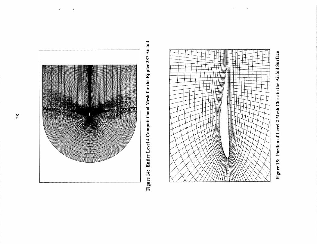
prohibitive. Views of the entirecomputationaldomainfor thethreetwo-dimensional

gridscanbe foundin Figures12through14. Figures15throl,gh 17showtheportion

of eachmeshcloseto the airfoil surfaceanddisplaythepackingof grid points in the

boundarylayerregion.

Two otherfiles arerequiredby ADPAC in orderto runa calculation,an input

file and a boundarydatafile. The input file containsparametersthat allow one to

scalethe non-dimensionalgrid. In the boundarydatafile, one canspecify theangle

of attackand how the boundariesof the grid are to be treated.A combinationof

parameterswithin the input andboundarydatafiles setthe flow conditions. For all

num_?,.rthe two-dimensionalairfoil performancecalculations,the freestreamMach _

was fixed on the horizontal straight sections of the outer boundary of the

computationalgrid. Total temperatureand total pressurewere fixed on the inlet

curved sectionof the outer boundary, and static pressure was fixed at the straight

vertical exit plane° A no-slip condition was imposed on the blade surface, forcing the

velocity at the blade to be zero. Because ADPAC is a compressible code, a freestream

Mach number of 0.20 was set. The Mach numbers for the experimental data were

generally below 0.10.

24

Eachgrid wasusedto calculatethe flow at Reynoldsnumbersof 60,000,

100,000and200,000while angleof attackwasnominally8.00°. Angle of attack was

set to match that given by the experiment. Figures 18 through 20 show the calculated

airfoil surface pressure coefficients plotted against the non-dimensionalized

chordwise position and compared to the experimental data. Good agreement between

the computations with the Level. 4 grid and the experimental data was seen even at a

Reynolds number of 60,000 which would have the longest separation bubble of all

three cases.

• Figure 21 shows a comparison of the calculated value of the lift coefficient as

a function of the inverse number of mesh points for each Reynolds number. As

Reynolds number increases, more grid lines must be packed towards the airfoil

surface to resolve the thinner boundary layer. The dimensionless distance of the grid

line away from the wall, y+, is defined by Schlichting in Reference 10 as:

+

y =

Y I "l_wallp

where y is the dimensional distance of the grid line away from the airfoil surface, x,,.,,,

is the shear stress at the wall, p is the fluid density, and v is the fluid kinematic

viscosity. The values of y+ for the first grid line of the Level 4 mesh at the quarter

chord point are 0.0624, 0.0915, and 0.1537 for Reynolds numbers of 60,000, 100,000,

and 200,000, respectively.

25

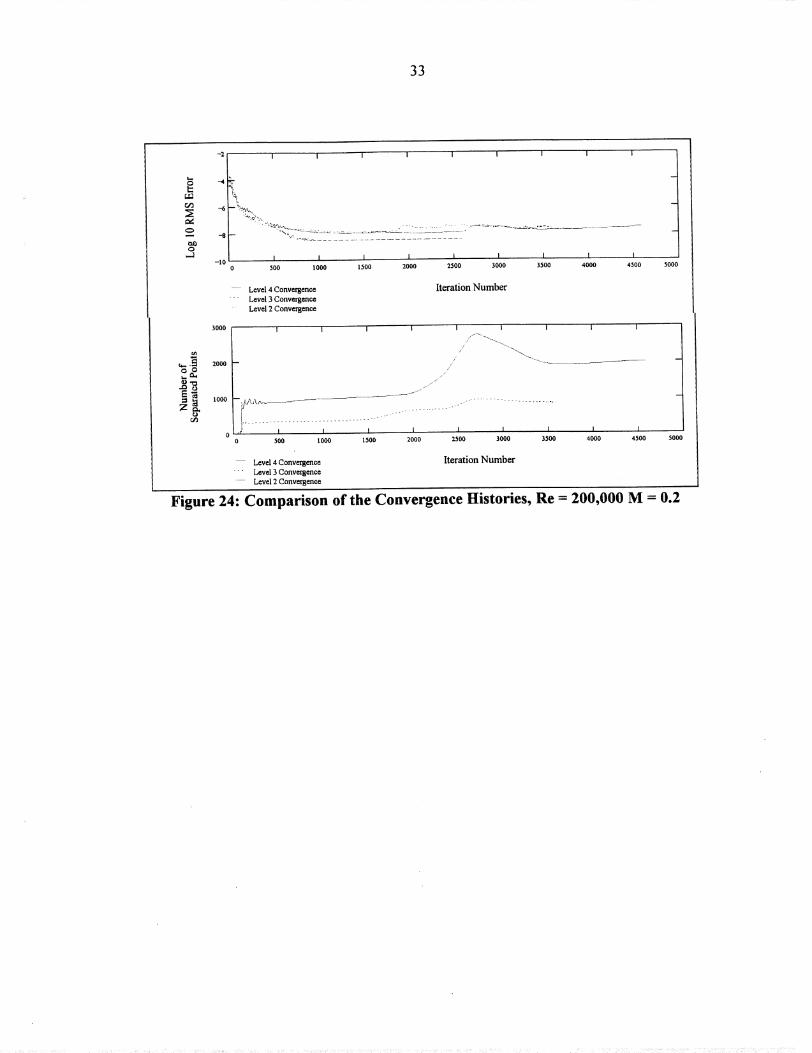
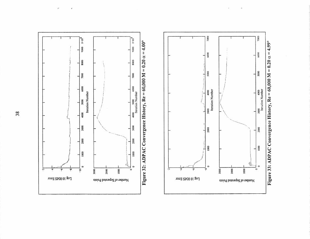
Accompanyingeach solution is a set of convergenceplots. Figures 22

through24 containtwo convergenceplots for eachsolution: the Root Mean Square

(RMS) Error, andtheNumberof Separatedpointsat eachiteration. TheRootMean

SquareErrorwasdefinedto be thesumof thesquaresof theresidualsof all the cells

in the mesh, the residualbeing the sum of the changesof the five conservative

variables,p, pu, pv, pw, andpe. TheADPAC definition of a separatedpoint wasa

cell whosevaluefor Vxwasnegative.Generally,for the low Machnumbercases,the

calculationwas run until the numberof separatedpoints seemedto be constantand

theresidualswerereducedby atleastthreeordersof magnitude.

The Level 4 grid was thenusedfor a seriesof calculationsat a Reynolds

numberof 60,000andanglesof attackrangingfrom -2.94° to 12.00°. The Level 4

grid was chosenbecauseof the good agreementbetween the surfacepressures

calculatedby ADPAC andthe experimentaldataat a Reynoldsnumberof 60,000

(Fig. 18). Lift coefficientswerecalculatedfor eachangleof attackandcanbe seen

comparedto the Langleyresultsin Figure25. Pressurecoefficientdistributionsare

presentedin Figures26 through31 for eachof the coloredpoints in Figure 25.

Figures32 through37 are the correspondingconvergencehistoriesfor eachof the

selectedADPAC calculations. Sincethe viscousdragresult wasunavailablefrom

ADPAC, it wasestimatedby calculatingskin friction dragonbothsidesof aflat plate

drag(Ref. 10):

26

Cd=1.328

The total of the viscous plus pressure drag coefficients were then plotted against the

Langley data and are shown in Figure 38.

There was generally good agreement between the ADPAC calculated values

and the experimental values. Examination of the plots shows that ADPAC, like many

other numerical analysis codes, was unable to predict the laminar stall that was

measured at Langley at angles of attack from 3.00 ° to 7.50 ° . The marked increase in

measured drag in this region was also unpredicted by this version of ADPAC. For

angles of attack less than 8.01 ° there is not good agreement between the calculated

and experimental data near the trailing edge with ADPAC predicting recompression

farther upstream than was seen in experiments in the Langley LTPT (Fig. 26 - 29).

Agreementbetween the ADPAC prediction and the experimental results at the trailing

edge improves at ar_gles of attack of 8.01 o and greater (Fig. 30 - 31).

27

=J=

/!!/

!!r/

,, ,.,_

i

Figure 12: Entire Level 2 Computational Mesh of the Eppler 387 Airfoil

Figure 13" Entire Level 3 Computational Mesh for the Eppler 387 Airfoil

00

Nomll

oml

N

m_

c_

C_oN

c_

E

c_

c_

_NonU

c_

_Oomu

mu_oj_

_uollt

c_

C_

v_

c_

omU

29

Figure 16" Portion of Level 3 Mesh Close to the Airfoil Surface

Figure 17" Portion of Level 4 Computational Mesh Close to the Airfoil Surface

30

-5 I I I I I I I ! I

0 ,_ ........ _..____,_.____._:_ __,_.... ___-___,--__-_----__---=--_----"_

1 "_"_i "_'__

2 I I I I I I ! I0 0.1 0.2 0.3 0.4 0.5 0.6 0.7 0.8 0.9

o Langley Data, M = 0.05

Lovol 4 Mosh, M = 0.20

-- Lovol 3 Mesh, M = 0.20

-- Lovol 2 Mesh, M = 0.20

X/C

Figure 18: Pressure Coefficient vs. Non-dimensional Chordwise Position and

Different Computational Mesh Densities, Re - 60,000 and _ = 8.01 °

-5 I I I I I I I ! i

4i _

3

-2!_::_. ___ ___

1 I I I I I IT_

20 0.1 0.2 0.3 0.4 0.5 0.6 0.7 0.8 0.9 1

O Langloy Data, M = 0.08

Lovel 4 Mesh, M = 0.20

-- Lovel 3 Mesh, M = 0.20

- " Lovel 2 Mesh, M = 0.20

X/C


Different Computational Mesh Densities, Re- 100,000 and _ - 8.00 °

31

<> Langley Data, M = 0.06

Level 4 Mesh, M = 0.20

Level 3 Mesh, M = 0.20

- Level 2 Mesh, M = 0.20

X/C


Different Computational Mesh Densities, Re = 200,000 and _= 8.00 °

rj

1.5 n

1 --

0.5 --

o

--o- Re = 60,000

+- Re = 100,000

-_ Re = 200,000

l/(Number of Mesh Points)

0.001

Figure 21- Calculated Lift Coefficient vs. Inverse of Number of Computational

Mesh Points at ot - 8.01°

32

-2 It-O

12: -4 ¸

rj3

o

_) -8

Q

..J

-I0

4000

Q O

Z_

I I I I I I I

<h

...... _..- . -.

u

i I I I I I I

0 500 1 000 ! 500 2000 2500 3000 3500

Level 4 Convergence

.... Level 3 Convergence


Iteration Number

4000

.

0 500

i I I I I I

/ ......../

/

/

........ :S < .............................................................................

I I .! I I !

1000 1500 2000 2500 3000 35004000

Level 4 Convergence


Level 2 Convergence

Iteration Number

Figure 22- Comparison of the Convergence Histories, Re = 60,000 M = 0.2

-2 I I I I I I

t_

r,,r.l

0

e_ -8

0

.-I

c¢I

x 6.

-I0

4000

2000

I I I I I

500 1 000 1500 2000 2500

I I

3000 3500

Level 4 Convergence

-- Level 3 Convergence

Level 2 Convergence

Iteration Number

I I I I I I I

I_&]<<-- ..... ,-"

0 50O 1000

/

/

I I I I I

1500 2000 2500 3000 3500

I

Level 4 Convergence

'- Level 3 Convergence


Iteration Number

4000

Figure 23: Comparison of the Convergence Histories, Re = 100,000 M = 0.2

40O0

33

L--

r_t3

C/3

O

r_q

L.

r./3

-2 I I I

-'-,_. _,_

'-. i'!):),._.._.,_...._

I I I-I0

0 500 1000 1500

I I I I i I

I I I I I I

2000 2500 3000 3500 4000 4500 5000

Level 4 Convergence

--- Level 3 Convergence- Level 2 Convergence

Iteration Number

3000 I I I I I I I

2000 / _"_-

//yJ

j_

...................................._..................................0IJ ......... i I , I _ _ I

0 500 1 000 1500 2000 2500 3000 3500

I

!

4O00 4500

Level 4 Convergence

-- Level 3 Convergence

Level 2 Convergence

Iteration Number

5000

Figure 24: Comparison of the Convergence Histories, Re = 200,000 M = 0.2

"::::t"

! i i i i l t__

IO 'lu0!__0o3 U!l

(Dr.,,_

o¢.-,I,::5It

o It ._

g3

r +f

r_

6Jl

0

_----,,,_

tt

0

r_

!j_ee

¢,q

e_

35

-5

-4

-3

I i I i I I I I I

o 0 o o o o o

I I I I I I I I I

O.1 0.2 0.3 0.4 0.5 0.6 0.7 0.8 0.9


ADPAC Calculation, M = 0.20X/C

Figure 26" Pressure Coefficient vs. Non-dimensional Chordwise Position,

Re = 60,000 tx = 4.00 °

I I I I I I I I I

0-0 0---0....0--_-0.......-0....0--'--0----0.....0---0 ....0 0 0

0_ - ..... 0 0

G¢oo._---o--o_o -o_---o ---o--o---o---o-o::---:_---

I I I I I I I I .......I I

0.1 0.2 0.3 0.4 0.5 0_6 0.7 0.8 0.9

O Langley Data, M = 0.05

ADPAC Calculation, M = 0.20

X/C

Figure 27: Pressure Coefficient vs. Non-dimensional Chordwise Position,

Re = 60,000 c_ = 4.99 °

36

-4-

-3_

-2-

-l

0

l

! I i I

-_:£00 0 0

,-

0 0

<Z__. 0

i I i I I

0 o o o 0 o 0 o o o

o _0 0 0 ___0___0 _.0_ 0 0- - 0-_--

2 I I I I I I I I I

0 O. 1 0.2 0.3 0.4 0.5 0.6 0.7 0.8 0.9



X/C


Re = 60,000 a = 6.01°

I I I I I I i I i

-2_O

O- -0 -0 ...._ .....0 ....0 -0--0- 0 0 0

0

0 0 0 0O-

_O__O--O--_O----O_-_----O----O--O----O--O---O-----O----O----O

if

2 I I I I I I ! ! I ,0 0.1 0.2 0.3 0.4 0.5 0.6 0.7 0.8 0.9

X/Co Langley Data, M = 0.05


-.$-__.:_

Figure 29" Pressure Coefficient VSoNon-dimensional Chordwise Position,

Re- 60,000 tx = 7.00 °

37

-5 I I I I

_2I%o<_. _ o

__|,.m

I I I I I

--0 .... O_0 _ O 0

o--o.....o o ---_----

I I l I I I I I I I

0 0.1 0.2 0.3 0.4 0.5 0.6 0.7 0.8 0.9

X/Co Langley Data, M = 0.05



Re = 60,000 t_ = 8.01°

o

I I I I I I I I

I I I I I l I I ,

0.2 0.3 0.4 0.5 0.6 0.7 0.8 0.9


ADPAC Calculation, M -0.20

X/C


Re = 60,000 c_ = 9.00 °

oo

%

! g

I °- g"l O0

- i -

- i -i

/

eet

/ °< "-_

//0

o

t-,

Z§ =

c_

J0_] SI_IOI l]0l

I

1

- //

/

(\

\

\

",.,\

'l I .......

1I-tt

L-

g g oo oeq --,

%

slu!0d p01_.1_d0Sj0 J0qtunN

-' O

oG", II

oo ¢'q

II

g oo X,D,,O

g..

Egzo

.o ;;_"_ g.," O

....,O_..,

,, =¢De_

o g:lo

I.

o =Io oo

" L)

o .<o

_ gh

° gl

I.=

om_

i I

..

l'

/

-3

5i

_ I ..-----7 i"

J0_t SI_ O[ i]0"I

,, Ez

.o

IN¢J

0 "-'0e_

[ I J '

m

-\

-._ ..

I [ "=--:o° § g °0 oeel _ ,-,I

g

oo

0o

ob-_-_

z

0._

L.

oN

m

\ ooo

ooo

"_7.

o

slu!0dp01_J_d0sj0 ._0qtunN

0

o'xO',,

II

¢.q

!i

II

e,,

I.o

'4_

om

=

¢12

I....¢D

=OL)L).,¢gh

.<oo

¢DI.

olmal

39

O

I:::

0'2

O

O

-4

-6

-I0

I I I I I I I

I I I I ! I I

0 I000 2000 3000 4000 5000 6000

IterationNumber

7000 8ooo

r._......

O

C_t...

c_

r./D

o

l..,,

E

Z

4000

2000

I I I i i I !

/.

/

I I I ! I ! !

0 1000 2000 3000 4000 5000 6000 7000Iteration Number

8000

Figure 34" ADPAC Convergence History, Re = 60,000 M = 0.20 c_ = 6.01°

O -4

o"2

-6O

O -8

-10

I I i I i i i I

I I I I I I I I

1000 2000 3000 4000 5000 6000 7000 8000

Iteration Number

9ooo

°..O

O"2

OL.

E

Z

4ooo

2000

I I I I I i I I

,- t-_---._.__._... __.... .

i

/

:

/

/

/£

//

! I I I I I I !


9000

Figure 35" ADPAC Convergence History, Re = 60,000 M = 0.20 ct = 7.00 °

4O

O

C_O

C)

...,9

O

O

CL_

Z

2L-4

-6 L_"_,..,,

0 500

I l

I I

1000 1500

I I I i

l I I

2000 2500 3000

IterationNumber

I

3500 4ooo

4000

2000

!,:l.:lj\:<.

'

/

//

/

./

J

I I I i [

I I I ! I ! I

500 i 000 ! 500 2000 2500 3000 3500Iteration Number

4000

Figure 36: ADPAC Convergence History, Re = 60,000 M = 0.20 _ = 8.01°

-2 i I

0

C/2

0

E

Z

i.i0 -4

_2

-6

_0Q -8

-10

I I i I I

I I I I I I

1000 2000 3000 4000 5000 6000

Iteration Number

60OO I I I I i I I

4OOO

2000

,/

m ./

I

/..

/

/

./

: I I I

0 1000 2000 3000

I

7000

I I I !

4000 5000 6000 7000Iteration Number

8000

8000

Figure 37" ADPAC Convergence History, Re = 60,000 M = 0,,20 tx = 9.00 °

41

L)

°v,-I

O

OL)

• v=,,l

1.4

1.3

1.2

I i i I i I I i i

- <>_----o-<>--_<>----

\<>

4"

| --

0.9--

0.8--

0.7--

40.6-- '

t/

0.5-- _

/

0.4 '

I!,,,

0.3 It"

0.2 -!_

t/

0"F

//

/

/

/

0

/' •

o' "oo----_

//

/,o

/

0/

B

\

/

@

t /,, .4.- 4" /

/

t"

'4- ....

' 0

I I ! I I ! I I !

0.03 0.04 0.05 0.06 0.07 0.08 0.09 O. 1 O. ! I

Drag Coefficient, Cd-o- Langley Data, M = 0.05

-t-- ADPAC Calculation, M = 0.20

0,12

Figure 38: Comparison of Measured and Calculated Drag Coefficient versus

Lift Coefficient for Re = 60,000

CHAPTER 4

Propeller Design Using Experimental Airfoil Data

Fundamentals of propeller theory were established by Glauert as early as 1926

(Ref. 11). Primarily because of the absence of computers, solutions of Glauert's

analysis theory could only be obtained after making a number of simplifying

assumptions. While the basic theory has remained the same, Adkins and Liebeck ::,

have recently removed most of the assumptions, establishing iterative design and -

analysis procedures which, with the aid of a computer, can solve for the geometry or

performance of a propeller quickly.

Glauert used a combination of momentum and blade element theory to model

the propeller. In the momentum theory, the flow upstream and downstream of the

propeller is considered to be a potential flow, that is, the fluid is assumed to be

inviscid, incompressible, and irrotational. The propeller is thought of to have a large

number of blades so that it could be represented as an 'actuator disc.' Further,

Glauert assumed that the axial velocity passing through the actuator disc is

continuous, and the pressure over the surface of the disc is constant although it

increases discontinuously after passing through the disc.

Glauert used a blade element theory to get more detailed information on the

performance of the propeller blades. In this theory, flow past any blade airfoil section

is assumed to be two-dimensional and the lift at each section results from the

circulation of flow around the blade. Trailing vortices are shed from the blade and

42

43

passdownstreamin a helicalvortexsheet,andinterferencefrom these vortices cause

the rise in axial and radial velocities through the propeller. Forces on the blade

elements can be resolved, and once integrated over the length of the blade, ultimately

yield propeller thrust, power, and efficiency.

Strip-theories other than Glauert's momentum-blade element theory exist,

differing only in the way in which the induced velocities are found (Ref. 12). It was

Adkins and Liebeck (Ref. 2), however, who published algorithms for iterative design

and analysis procedures in which nlany of the simplifying assumptions were

eliminated. Specifically, Adkins and Liebeck's procedures eliminated the small angle

assumption, and the lightly loaded assumption in the Prandtl approximation for

momentum loss due to radial flow. Their procedures continue to neglect contraction

of the wake. If the vortex sheet is assumed to form a rigid helical surface, the Betz

condition for minimum energy loss will be met. A design will be optimized when

viscous as well as momentum losses are minimized. To do this, the designer should

specify that each section operate at an angle of attack corresponding to the maximum

lift-to-drag ratio.

Adkins and Liebeck give eleven steps describing the iterative design

procedure in Reference 2. Briefly, the parameters specified at the beginning of a

design are: power, hub and tip radii, rotational speed, flight velocity, number of

blades, number of radial stations along the blade, and either a lift coefficient or chord

length distribution along the blade. The program iterates to find blade twist angles,

44

chordor lift coefficient distributions (depending on which was specified in the input),

radial and axial interference factors, Reynolds number, and relative Mach number.

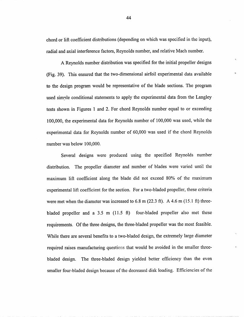
A Reynolds number distribution was specified for the initial propeller designs

(Fig. 39). This ensured that the two-dimensional airfoil experimental data available

to the design program would be representative of the blade sections. The program

used sim,91e conditional statements to apply the experimental data from the Langley

tests shown in Figures 1 and 2. For chord Reynolds number equal to or exceeding

100,000, the experimental data for Reynolds number of 100,000 was used, while the

experimental data for Reynolds number of 60,000 was used if the chord Reynolds

number was below 100,000.

Several designs were produced using the specified Reynolds number

distribution. The propeller diameter and number of blades were varied until the

maximum lift coefficient along the blade did not exceed 80% of the maximum

experimental lift coefficient for the section. For a two-bladed propeller, these criteria

were met when the diameter was increased to 6.8 m (22.3 ft). A 4.6 m (15o 1 ft) three-

bladed propeller and a 3.5 m (11.5 ft) four-bladed propeller also met these

requirements. Of the three designs, the three-bladed propeller was the most feasible.

While there are several benefits to a two-bladed design, the extremely large diameter

required raises manufacturing question, s that would be avoided in the smaller three-

bladed design. The three-bladed design yielded better efficiency than the even

smaller four-bladed design because of the decreased disk loading. Efficiencies of the

45

three-bladedpropeller and the four-bladedpropeller were 85.3% and 81.5%,

respectively. Comparisonsof the propellergeometriescanbe found in Figures40

_ough 42.

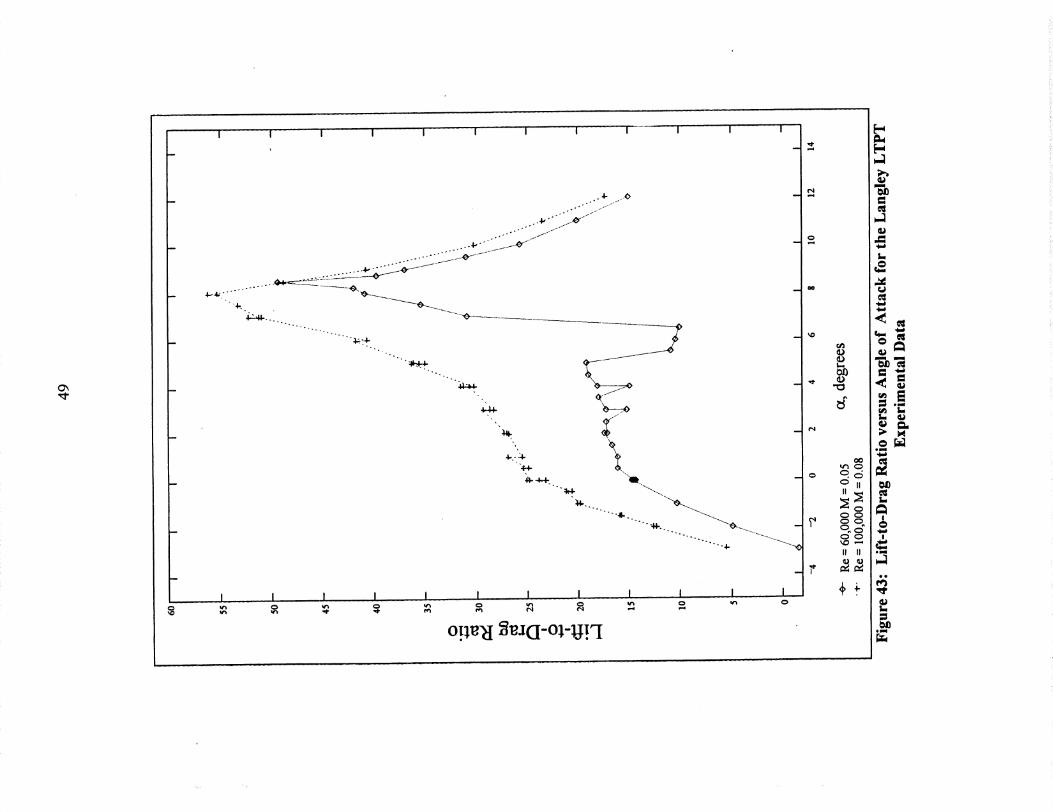
Examinationof the blade twist distributionsfor all threedesigns(Fig. 40)

showeda 'hook' in thecurveasthebladewastwistedthroughthe stalledportion of

the lift curve for the experimental data at the Reynolds number of 60,000 (Fig. 1).

Since viscous losses were not minimized in these designs, the three-bladed design

was optimized by relaxing the requirement that section lift coefficient be less than

80% of the maximum and specifying a constant lift coefficient corresponding to the

maximum lift-to-drag ratio point in the experimental data set (Fig. 43 - 44). Blade

twist, chord, lift coefficient, and chord Reynolds number distributions can be found in

Figures 45 through 47. While this eliminated the 'hook' in the twist distribution

(Fig. 40), it was clear that the lift coefficients near the hub would have to be

decreased in order to increase the chordlengths of the inboard sections. The exercise

of refining the hub sections was deferred to the next design trials.

The design studies using the Langley experimental data were useful in several

ways. These studies showed that the specified Reynolds number distribution did

yield a reasonable propeller geometry. With refinement, chordlengths of the inboard

sections could be improved and the hook in the twist distribution curve could be

eliminated. Knowing the Reynolds number and relative Mach number distribution

over the blade would help to account for compressibility effects that were so far

46

neglectedin the presentdesigns. As will be shownin the next chapter,ADPAC

wouldbeusedto makeperformancepredictionsfor theEppler387 airfoil operatingat

thesetransoniclow Reynoldsnumberconditions. Finally, the designstudieswere

usefulin identifying feasiblevaluesfor thepropellerdiameterandnumberof blades.

47

1.6-105 I I I I I I I I

1.4"10 5

"_ 1.2"I05

:::1

Z

1"105

¢D

8" 104

./

//

/

/"/'

/:

.-. //

///

/

//

/

6.1o 4 , I I

0.I 0.2 0.3

//

//

/

,/

/

I l l I0.4 0.5 n

r/Rtip

-,...,.,,

\,.

_ -\

\

I0.7 0.8 0.9 1

Figure 39: Design Reynolds Number vs. Non-dimensional Radial Position

9O

80 D

70--

60--

50--

40--

3O

I i I i i I I I I

<_L,

I I I .

0 0.I 0.2 0.3

_,:-'-...._

0.4 0.5 0.6 0.7 0.8 0.9 1

r/R.tip

-o- Blade Twist Angle, 2 Bladed Propeller, Rtip = 3.4 m

_'- Blade Twist Angle, 3 Bladed Propeller, Rtip - 2.3 m

+ Blade Twist Angle, 4 Bladed Propeller, Rtip = 1.75 m

Figure 40" Blade Twist A_gle (degrees) vs. Non-dhnensional Radial Position,

Designed Using Langley 2-D Experimental Data Only

48

t.,O

0.8

0.6 m

0.4

0.2

I I I I I I I I I

I I

0.1 0.2

.1[ --_" ._.

I I I ! I,

0.3 0.4 0.5 0.6 0.7

-e- Chord, 2 Bladed Propeller, Rtip = 3.4 m r/Rtip

_ Chord, 3 Bladed Propeller, Rtip = 2.3 m

-+- Chord, 4 Bladed Propeller, Rtip = 1.75 m

u

! ! _-LJ

0.8 0.9 1

Figure 41- Chord (meters) vs. Non-dimensional Radial Position,


O

OO

rj

° _,,,I

1.2

0.8

0.6

0.4

0.2

I i I

/ °.

//.,// ." /al_..

._/ . . / / "

I I I

0 0.1 0.2 0.3

i I I I ' ' I I ]

/..-" z<.-_ //

I I I ! I I

0.4 0.5 0.6 0.7 0.8 0.9

r/Rtip

-e- Lift Coefficient, 2 Bladed Propeller, Rtip = 3.4 m

'< LiR Coefficient, 3 Bladed Propeller, Rtip = 2.3 m

+ Lift Coefficient, 4 Bladed Propeller, Rtip = 1.75 m

Figure 42: Lift Coefficient vs. Non-dimensional Radial Position,


C_

....... °-.

..

".H-

/-"

":k4- _"

.... 4,.... _"

"4-

........ j _

50

1.2

1.18

_D0,.._ 1.160

0 1.14

1.12

1.1

I I I i I i I I

I ! ! I ! ! ! !0.1 0.2 0.3 0.4 0.5 0.6 0.7 0.8 0.9

r/Rtip

Figure 44- Lift Coefficient vs. Non-dimensional Radial Position, Three Bladed

Design, Tip Radius = 2.3 m, Langley 2-D Experimental Data Only

90

80

70

60

50

400.1

I I I I i I i i

<>

<>

<>

<><>

<>! ! I ! ..... ! ! I I. °oc_

0.2 0.3 0.4 0.5 0.6 0.7 0.8 0.9

r/Rtip

Figure 45- Blade Twist Angle (degrees) vs. Non-dimensional Radial Position,

Three Bladed Design, Tip Radius = 2.3 m, Langley 2-D Data Only

51

O

L)

0.8

0.6

0.4

0.1

I I i i i l I I

O •

O -O

"oI ! ! ! I ! ! !

0.2 0.3 0.4 0.5 0.6 0.7 0.8 0.9

r/Rtip

Figure 46: Chord (meters) vs. Non-dimensional Radial Position, Three Bladed

Design, Tip Radius = 2.3 m, Langley 2-D Experimental Data Only

1.5' 105 I i I I i i I i

1.10 5

r.,_ ¸

o

_, 1o4

_ loooo

.<>

.............................___o.,_:::i........................................................__.__..._._ooo,./

.0 0

//

I l I I l I l I

0.1 0.2 0.3 0.4 0.5 0.6 0.7 0.8 0.9

r/Rtip

Figure 47: Reynolds Number vs. Non-dimensional Radial Position, Three Bladed

Design, Tip Radius = 2.30 m, Langley 2-D Data Only

CHAPTER 5

ADPAC Two-Dimensional Aerodynamic Predictions

ADPAC two-dimensional results were combined with the strip theory design

program in an effort to account for compressibility effects so far neglected. To do so,

the blade was divided into four segments. The specified propeller Reynolds number

distribution and the resulting Mach number distribution were used to identify an

average value of the Reynolds number and the Mach number for each segment

(Figure 48). These values are listed in Table 3.

Table 3. Reynolds Number-Mach Number Combinations

Segment Reynolds Number Mach Number

1 60,000 0.45

2 100,000 0.55

3 100,000 0.65

4 60,000 0.75

The Level 4 computational mesh of the Eppler 387 (Figures 14 and 15) was

used to generate section performance predictions for a range of angles of attack for

each of the Reynolds number-Mach number combinations in Table 3. Surface

pressure coefficients were compared to Langley experimental data that had been

corrected for the elevated relative Mach number using the Prandtl-Glauert

compressibility correction (Ref. 13)

(f_P corrected --"

Cpo

52

53

whereCpo is the value of the incompressible pressure coefficient and M_ is the free

stream Mach number. The pressure coefficients calculated with ADPAC were in

turn integrated to yield lift and pressure drag coefficients. The total drag coefficient

was found by adding the viscous drag component once again estimated by drag on

both sides of a flat plate given by Schlichting in Reference 10"

Lift and drag curves are found in Figures 49 through 52. Plots of the surface pressure

coefficients and corresponding ADPAC convergence history plots for angles of attack

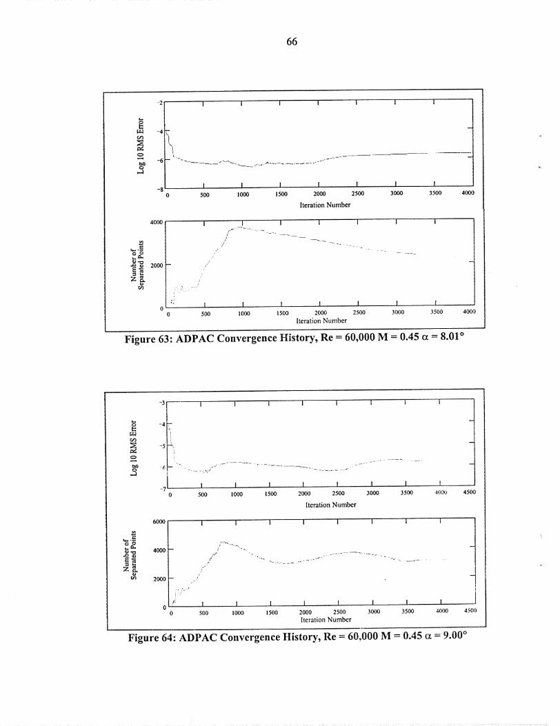
of 4 °, 5 °, 6 °, 7 °, 8 °, and 9 ° are given for Segment 1 in Figures 53 through 64,

Segment 2 in Figures 65 through 76, Segment 3 in Figures 77 through 88, and

Segment 4 in Figures 89 through 100. Where appropriate, the number of supersonic

points at each iteration are included in the convergence history plots.

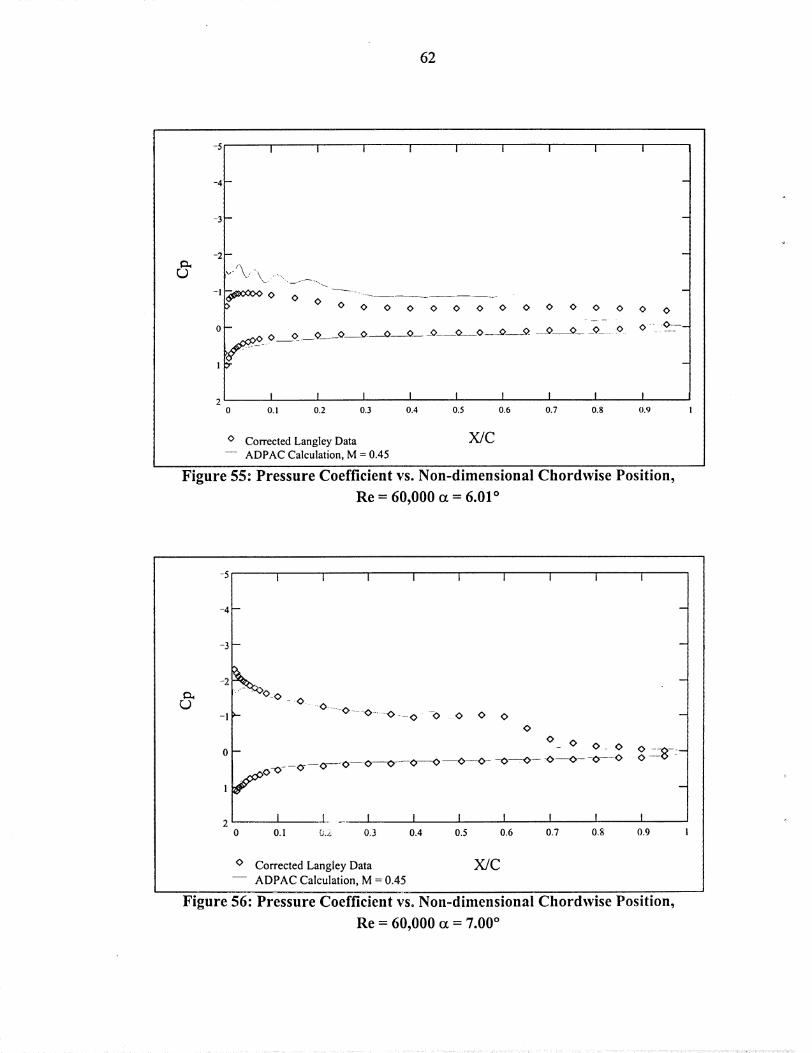
An examination of the Segment 1 results at Re = 60,000 and M = 0.45 shows

that agreement between the ADPAC calculated values and the corrected Langley data

is generally good. The calculated suction side pressure recoveries are sharper than the

corrected data would suggest for low angles of attack. Just as was seen in the code

validation, ADPAC did not predict a laminar stall at angles of attack between 5.00 °

and 6.49 ° . For angles of attack between 7.51 ° and 12.00 ° , there appears to be

periodic shedding of the separated shear layer, similar to that reported by Pauley, et.

al. in Reference 4. Figure 101 shows the pressure distribution over the airfoil at an

angle of attack at 8.01 ° and the streamlines shown in Figure 102 for the same

54

conditionindicatemultiple separationandreattac_ent points nearthetrailing edge

of thesuctionside. Theseresults,aswell asall of theotherADPAC resultspresented

here,arenot time-accurate,but representthe steadystateflow solutionachievedwith

local time stepping.Thelocal time steppingtechniqueadvanceseachcell in time by

an incrementequal to the maximum allowabletime step for that cell. Generally,

largercellsawayfrom aboundary,layerwill havealargertime stepthansmallercells

closerto asolid surface.

Examinationof the resultsin Segment2 for a Reynoldsnumberof 100,000

anda Machnumberof 0.55showsthattherewasalsogenerallygoodagreementfor

anglesof attackrangingfrom -2.88° to 4.00°. Shockwavesnearthe leadingedgeare

seenin theADPAC predictionsfor anglesof attackgreaterthan6.00°. Full stall is not

predictedat 14.04°. The Prandtl-Glauert correction is inadequate for these conditions

and an experiment would be needed to validate these predictions.

As Mach number is i_creased from 0.55 in Segment 2 to 0.65 in Segment 3,

more differences are seen between the corrected experimental data and the ADPAC

predictions. Shock waves are seen for all angles of attack above 3.00 ° , and like in

Segment 2, full stall of the airfoil at 14°04 ° is not predicted by ADPAC.

Representative of the tip sections, Segment 4 with a Reynolds number of

60,000 and a Mach number of 0.75 shows gross differences between the corrected

Langley data and the ADPAC predictions as would be expected from the inaccuracy

of the Prandtl-Glauert correction at these conditions. ADPAC solutions indicate that

55

theairfoil is unableto producea strongleadingedgesuctionasaresult of the shock

wavesseenateveryangleof attack.

56

1.5 I ' l i i • _. I I 0.89i1.4-- 0.25 + 0._5 + --

..

: d- -I-1.3-

.p1.2-

1ol- -+ [Segment2 ] [Segment3 ] _

........................................................................................................... + .......... -_0.9-- +

n

.......... 0 .....

-Isegme°t'i

........ 0 .....

@

^ _.00

-I-ra

0.8

0.7

0.6

0.5

0.4

0.3

0.2

0.1

0I ! I . I I !

0.1 0.2 0.3 0.4 0.5 0.6 0.7 0.8 0.9

-O- Relative Mach Number

+- Reynolds Number/100,000

Figure 48" Segmented Reynolds Number and Mach Number Distributions

:: .: :: : :.:::_::.:i:i ..... ._: =============================

57

4,..t

_D.vu{

O

(D

1.4

1.3

1.2

l.l

l

0.9

0.8

0.7

0.6

0.5

0.4

0.3

0.2

0.1

0--"

"-0.1

I I i I i I

>{ " 0/"/

I Ol /

//.. .. I" -

//_< d" _"".- t-/

/ y,- +1-/_ // ./

,,." ,_

,, .,," _%>

/ o_

//

•• /_//

•• _i///

t, '" L /

¢

.//_

///'/

//

//

/

/" O/"

// o .,-.........

-/'O00. ,// " /

/ _ /":." o

..

o.__.

I

//

o I I I I I--4 --2 0 2 4 6

cz, angle of attack, degreeso Re =60,000M = 0.2

LeastSquaresPolynomialFitofRe = 60,000M = 0.2Re =60,000M = 0.45

_ LeastSquaresPolynomialFitofRe =60,000M = 0.45* Re = 60,000 M = 0.75

.... Least Squares Polynomial Fit of Re = 60,000 M -- 0.75

I I8 10

Figure 49: Comparison of ADPAC Predicted Lift Coefficients at

Re = 60,000 and M = 0.20, 0.45, 0.75

_ : : ::?-: _: ":: Y::: :_ : " ?::_::::::- .... :/": :"/:Y ,, /:i_ i: ::i : :71:?!: I::I:::i:UZI_:I:L ::i:?:!?:::.... I"Y!:::!::¸ "_i:::::i:L U::III!:I:":i:::Y::Z_:::I__L:;: :?Z:i:iG::!!_ii_i_:_!:i/i:!::!!::i:!:!:!:::L:::!:i::ii:!_::?::iiii::!i!i;::¸::!:::ii:::Z:ii!:_:::::_:_::'::i::_:::::::i::::::_

58

C

t,-m

0.18

0.16

0.14

0.12

0.08

0.06

0.04

0.02

-4

I-

I I8 I0 12

I I I I I"2 0 2 4 6

or, angle of attack, degreesRe = 60,000 M = 0.2Least Squares Polynomial Fit of Re = 60,000 M = 0.2Re = 60,000 M = 0.45Least Squares Polynomial Fit of Re = 60,000 M = 0.45Re = 60,000 M = 0.75

' Least Squares Polynomial Fit of Re = 60,000 M = 0.75

Figure 50: Comparison of ADPAC Predicted Drag Coefficients vs Angle ofAttack at Re - 60,000 and M = 0.20, 0.45, 0.75

59

¢)-v.-¢

¢)O

°_

1.4 I I I I I I

0.7

0.6

0.5

/ ,,,/

,,I/./ ,,

_I ,//"/:/

/

/,{

//

//

I /N:'

//

// /

o Re=I00,000M=0.55

I I I I4 6 8 I0

or, angle of attack, degrees

Least Squares Polynomial Fit of Re = 100,000 M = 0.55)< Re = 100,000 M = 0.65

Least Squares Polynomial Fit of Re = 100,000 M =0.65

\\

Figure 51" Comparison ofADPAC Predicted LiftCoefficientsat

Re = 100,000 and M = 0.55,0.65

60

O

O

0.2

0.18

0.16

0.14

0.12

0.08

0.06

0.04

0.02

I I' I I I I I I I

//

X /,,

/ .....(>

/ ,/

/ /.

/L,. '°.._

! I I I ! I I,

-4 -2 0 2 4 6 8 10

(z, angle of attack, degreeso Re = 100,000 M = 0.55

Least Squares Polynomial Fit of Re = 100,000 M - 0.55

Re = 100,000 M = 0.65

-- Least Squares Polynomial Fit of Re = 100,000 M = 0.65

t/

/

//

/

/ o/:

///

//.

/:

///

/./

o .,/o./

/"

/

/.

!

II

II

//

/

/

//

//"

/'

/

.'/.

,/

I I12 14 16

Figure 52: Comparison of ADPAC Predicted Drag Coefficients vs Angle ofAttack at Re = 100,000 and M = 0.55, 0.65

61

I I I I I I I i I

! ! ! I ! I ! ! ! '

0 0.1 0.2 0.3 0.4 0.5 0.6 0.7 0.8 0.9 I

O Corrected Langley Data


X/C

Figure 53- Pressure Coefficient vs. Non-dimensional Chordwise Position,

Re = 60,000 t_ = 4.00 °

I I I I I I I I i

I I I ! ! I ! I !

0.1 0.2 0.3 0.4 0.5 0.6 0.7 0.8 0.9

0 Corrected Langley Data

.... ADPAC Calculation, M = 0.45

X/C


Re = 60,000 tx = 4.99 °

62

I i I I I I I I I

_0 0 0> 0 0 0 0 0 0 0 0

o_om

0 0 0 0 0

__.

9_ ....0 0 __0 ....O_

0 0

O:......0---

I I I I I I I I I J

O.1 0.2 0.3 0.4 0.5 0.6 0.7 0.8 0.9 1



X/C


Re = 60,000 _ = 6.01 °

I I i I I I I i i

--_.._

--0.....0 ....0 ......0 ......0 --0 ...0- 0 0

0

O_ 0 O_ 0 0

_ _---^_-e_------_-_O-----O----0--0- -0---70-- 0----0---0---0 --0 "-_- :-__ V V V V --

I J........ I I I I I I I

0 0. I O._ 0.3 0.4 0.5 0.6 0.7 0.8 0.9



X/C

Figure 56: Pressure Coefficient VSoNon-dimensional Chordwise Position,

Re- 60,000 ct = 7.00 °

63

-5 I I I I I l l I I

0......0__ 0

-----0-----0-_0_._0- ',0 0 -_| i-,- \\ . . _

"'' 0 " \ /0

o- ,.° °""° "/° ° o°

_o-o---°--°--°--°--° ......o......o--o- --o--o -o--o-_o-'-o---o-- ---I u

2 I I I I I I I I I0 0.1 0.2 0.3 0.4 0.5 0.6 0.7 0.8 0.9

o Corrected Langley Data


X/C

Figure 57 • Pressure Coefficient vs. Non-dimensional Chordwise Position,

Re = 60,000 _ = 8.01°

-5 i I i I i I I I I

--4

--3 _

-2 -- ----..... --..... "'" 0

- | -- _ .f"_"_"- --

0- o_ o \o /o_o_ o..8......--¢_......O---0 ....0---0 ....0---0---0- .....0-- 0----0-----0-----0....._ 0-- -0....0

2 I ! I ! ! I ! ! I0 0.I 0.2 0.3 0.4 0.5 0.6 0.7 0.8 0.9



X/C


Re- 60,000 cx = 9.00 °

64

0

f._

r./2

.,.,,,,i

o -6

i I I I i I

I I I ! I I ! !

500 1000 1500 2000 2500 3000 3500 4000

Iteration Number

4500

3000

2000

1000

I I , _.._ I I i I I I..... .

.

- //

/

/

/

/ -._ -- _ - -._,__Y

,; J

0 500

-..._

I I I I I I I

1000 1500 2000 2500 3000 3500 4000

Iteration Number

4500

Figure 59: ADPAC Convergence History, Re = 60,000 M = 0.45 c_ =4.00 °

t/-Ir.,o -4

_o -6O

-8

4OOO

t_

1.4

..t_ 2000

Or)

I I I i I I i I

it

I

0 500

I_'_............. __.._.. ,,---... , .

_ __ ...... _,' _ ..... ,--_, _,,..........................................

I I I I I I

1000 1500 2000 2500 3000 3500

Iteration Number

I ! I I i I i i

I

4O00

//

/

/,/

,/

/

4500

,_ I ! I ! I ! I !

0 500 i000 1500 2000 2500 3000 3500 4000

Iteration Number

4500

Figure 60: ADPAC Convergence History, Re = 60,000 M = 0.45 a =4.99 °

65

gr-Io'2

O,

-g_o

CCJ

4000

2OO0

I I I I i I

\\

\\-.

I2OO

I400

I I600 800

Iteration Number

! I

1000 1200

I I I I I I

.I-"

::I

/7 /f

p-

//:

/

/..i:

/- ....t

00 200 400 600 800 ! 000 1200

Iteration Number

1400

1400

Figure 61" ADPAC Convergence History, Re = 60,000 M = 0.45 Gt=6.01°

t-.O

I=: -4

O

-6

4000

c_

L_.

2ooozg.

r._

I I I I I I I I

I

.-_.o

.",'. -.-.- .........................

I ! I ! ! ! ! !1000 !500 2000 2500 3000 3500 4000

Iteration Number

0 500 450O

I I I I I I I I

--.--. _

,, ----- _....._.,_,_ ._

/.

t/

//

,/

/t

/

/XA ...... 'f

,:I I I I I ! I I !0 500 1000 1500 2000 2500 3000 3500 4000

Iteration Number4500

Figure 62" ADPAC Convergence History, Re = 60,000 M = 0.45 tz =7.00 °

66

O

I.r-1r./2

O

_0

O

-2 I I

I I !-8

0 500 Io00 1500

I i I I I

r--. _--

I ! I 1

2O00 25000 3OOO 35OO

IterationNumber

4ooo

4000

I-,

2oooO_

n

..,

/

,/

i: ":._''' " "-

0 500

I I

/

i i I 1

.-.

I I I ! I 1

1000 1500 2000 2500 3000 3500

Iteration Number

4000

Figure 63" ADPAC Convergence History, Re- 60,000 M = 0.45 c_ = 8.01°

O

I::

O'2

O

O

-3 i 1 I

m

!.,.

TL

I I i I I

I I I-70 500 1000 1500

t. .....

I ! I ! !_

2000 2500 3000 3500 4000

Iteration Number

4500

L..

Z _ca,

r,t)

6000

4000

2000

0

I I I

i' _''.--, ...... ,

f "-,..

(,,,,,'

I"

J

/

--._..

I I I I I

I I I I I I I I

500 1000 ! 500 2000 2500 3000 3500 4000Iteration Number

45oo

Figure 64- ADPAC Convergence History, Re = 60,000 M = 0.45 tx = 9.00 °

67

-3

-2

I I I I I t i i i

I I I I I I I I I0 0.1 0.2 0.3 0.4 0.5 0.6 0.7 0.8 0.9



X/C


Re = 100,000 tx = 4.00 °

L)

-4-

-3

-2 t..-

"1

o

1

I i I I i i I i 1

-0---0 ....0 .........0 .....-0-_-_0 .__/

7 o o

.......... O__ 0 ....

00_-0---_0----0 0 0_0 0 0------0---0_-----0 ---0

0 0 --0----0 --0 0 --_0- -

l l l I , l l l l I I

0.1 0.2 0.3 0.4 0.5 0.6 0.7 0.8 0.9 I

X/C

m

m

!i




Re - 100,000 tx = 5.01°

68

I I I I I I i i I

o o

I I I I I I I I I

0.1 0.2 0.3 0.4 0.5 0.6 0.7 0.8 0.9

X/Co Corrected Langley Data



Re- 100,000 ct = 6.00 °

I I I I I I I I I

_210%OOOo O --0

•--o....o....o ......o-_o ,, o--| _ -..._

o

- .o ....o- --o -o -o . o-o ---o- -0-

o------°----(r---°---°_-°----°_--°---:° _-o----o-- o----o---_ ....o- -o--o- -............oO

2 .............. i ....... I I I I I I I !0 0.1 0.2 0.3 0.4 0.5 0.6 0.7 0.8 0.9


ADPAC Calculation_ M = 0.55


Re = 100,000 tx = 7.00 °

69

I I I I I I I I I

-,0

......___.o.....o o o

o- __o____. ° _o-.._o_o_

--¢).....o---O-----O.....0----0---0-- 0---0-- "-0---0-- --0-----0--0

0 .....0.-__0-----0 ---0 -

I I I I I I I I I I

0 0. ! 0.2 0.3 0.4 0.5 0.6 0.7 0.8 0.9




Re = 100,000 cz = 8.00 °

-5

-2'-"

0--

1

I I I I I I I I I

"0

.....o o --oo

o-o

o

... o _..o._ o. -o_ --o_ -o_ --oo- -o ---

-.._-^----^----¢,,.----o---o---o---o- -o-- o----o----o --o .---o--_ v vv--

I I I I I I I I I

0.1 0.2 0.3 0.4 0.5 0.6 0.7 0.8 0.9



X/C


Re = 100,000 t_ = 9.00 °

....... :> ::: :: : :: ..... :::: ........ :'? .... .... • • Y!:/:;i, _ • • Y: .... ?!Y , :Y i:: ¸.:: ¸: : ......... ::!:::::......... : ::::::yi ¸,A:>::Yi:i!?::,:i.>; :::::/: :!:::::II:I::U̧ ?i:::::::::!:?::!i::(i/::i:Y:::,!!:::i::i:::!:::¸!!i:::ili:::il/,!!/:!:i!Y:::!i!::!i!:iii::::::::i:::::!:hli:!

7O

0

Q

I I I I I I I

I I I I I I I

500 1000 1500 2000 2500 3000 3500

Iteration Number

4000

Z _t_

r./2

3000

2000

lO00

I I I I I I I

//i

/

/

/

/

,-?...... I I l I I I i


4000

Figure 71" ADPAC Convergence History, Re - 100,000 M - 0.55 _ - 4.00 °

I--4O

r.P2

_U2O

-6

I I I I I I I

m

L]i

o.,

...... ----,-........

'_.,__ '-_ .,,.._ ../

! I I I ! 1 I

500 1000 1500 2000 2500 3000 3500 4000

Iteration Number

ta_

3000

2000

1000

I I I I I I I

//

/

//

//

/

_L I I

0 500 1000

I I I I _L..._

1500 2000 2500 3000 ."__,00 4000

Iteration Number

Figure 72" ADPAC Convergence History, Re = 100,000 M = 0.55 c_ = 5.01°

71

i.,,o

-21 i I i i i i Iu,.] L

° •-8 I ! I I I I

,I. ,4000.

400 I I i i i i i=

OL.

._'_ 200 ;_,,,

0 "" I I I I I I I.1., .4000.

400O I I I I I I i

_._O '

_,., /_'-----.

.__ 2000 ,, .................................

Z o'J ,/

m I ! I ! I I I0

0 500 1000 i 500 2000 2500 3000 3500 4000Iteration Number

Figure 73" ADPAC Convergence History, Re = 100,000 M = 0.55 cz = 6.00 °

-2 I Ii..,O

-4

-6 _.,.--, .... _ ..... _. _ jr--

O

-8 I I,.lj

.,..,=

°,.,

r_

I i 1 I I

I ! ! ! !

IO00/ I I I I I I

k500 /..__i "_

o I ""I f I ! \r -/,-L

.400q

.400(

_l 4000] I i I i I I I

_ 2000 // ....... "- ...................

O '

m i ! I I I ! !0

0 500 1000 1500 2000 2500 3000

Iteration Number3500 4000

Figure 74" ADPAC Convergence History, Re = 100,000 M = 0.55 _ = 7.00 °

¢,q

.._=

lt

i -F1

'L

t

/

I

1it -J

o"OO

......... i ...........

'h/

.,r

../"

'k.,

),,

I

,

"-,..)

/

.=_ ¢

/

_.j _

_<t .....q ...... I --0

0 0

_°-u_ISPf'd01 i_°q s)u!od 0!uosaodnsjo aoqtun N

O

t

\,

1

t

("

_ 1 ..

/)

/f'

\.

° § °oo

slu!od pole.led:) Sjo JoqtunN

Oot¢-)('-4 l,=.

(1.)

E

Z

§._gg.=(1.,)

.....

oo

0

00

II

It

e-,

II

o

Im

o

.<

<oo

om

]

I -

?

i -?

._:

[I

1

./.<

_ i,,-"I

a0aa/tSI,kr'dOI _0q

..... •

1'

// .-

//i

- [ -

\

/"1)

- I -/.

- 1 -

(.

0 0 0 '_

slu!od o!uos_adnsjo aoqtun N

r

/m

/

¢t

f

\

/

o o o

slu!od p01eaed0s20 aoqtunN

ooo 0

".

o

o

(I.)

E= II

t-0._

t... "--

o.4,,,,,)

._-

e_

o

- ¢D;;).

OL)

o

w-)

o®

¢D

0.0

73

-5i i i i i i i i i

_CCO0 0 ....¢ _ _0=____ "

> , " o o/ o

/- 0 O --

o o o --o o o------o--o--o------o--o--o--o--o--o--o - o o --:--_--_

I I l l I l t l I

0.1 0.2 0.3 0.4 0.5 0.6 0.7 0.8 0.9



X/C


Re = 100,000 ct = 4.00 °

I I i i I I I I I

-3-

-2 _

_¢oo oo---o

-| - /

/

/

0-

/6>0_0 0 0 0

1>

0 0 "\0 0 0 0

..--. __

.-- _ ___

-0 ....0 0 ....0__--

0 0 "---0 0 0 0 0 0 0 O-- -0-------0_0 ....0-'--0-

I I I l I l I t I q

0 0.1 0.2 0.3 0.4 0.5 0.6 0.7 0.8 0.9



X/C


Re = 100,000 ot = 5.01°

74

-4"-"

I I i ! I I I i I

-_O_o O

_- ...... --_

/

--/

>,/

. " ..\_

0 0 _0 0 0 0 O

\,_/': 0

..........-- -0 . 0-- -0- -0 ....O- 0 ....

0 -_----0 0 0 0--0---0_0 ----0-_0-" 0 0 0

I l

0.1 0.2

I I ! I I ! I

0.3 0.4 0.5 0.6 0.7 0.8 0.9




Re = 100,000 o_= 6.00 °

-5 I I I I I I I I I

-4

- o_ _ o_ --0 0 ......0--7_-

0 ' 0--0-----0-----0_- 0 0 .....0--

-3

-2 / 0 0 0 0 -0 0 0 • 0 0 0 0

'" ....0 -0_

..---_-o---6_,__o -0 o-- o o o o-....._._ :

lr_O_" _ i ......

2 I I i i I I I

0 0.1 0.2 0.3 0.4 0.5 0.6 0.7 0.8 0.9



X/C

Figure 80- Pressure Coefficient VSoNon-dimensional Chordwise Position,

Re = 100,000 tx = 7.00 °

....... . : ..... ...... :: .... : : ::: :: :: :... : : : : : . ..... ..... . .... ::: ..... , ......: :: : _ . :::: :: :::: : .: :: ::: ::::::::::::::::::::::::::::

75

-5 I I i I I I I I I

-4

.... -....... -----_____._O___O_ -i / o

,......

(_<:_0 0 0 0

0 0

00

0.................. 0 o

o°---°- o

0 O----_---<S ....o-- o ......o --o- -o- o _ o

I I I I I l I I I

0.1 0.2 0.3 0.4 0.5 0.6 0.7 0.8 0.9



X/C


Re = 100,000 _ = 8.00 °

I I I i I I I I I

>

0

-%_oo

m

o0 -"'0"

o'- 0

-" 0

_o o o o o o o o o

oo o

.... 0._o__o__

o ---o.....-0-- o-- o----o- -

0 0 - 0 ---_

-0....0 0 0

I I l I I I I I I

0 0.1 0.2 0.3 0.4 0.5 0.6 0.7 0.8 0.9



X/C


Re = 100,000 o_= 9.00 °

76

,. -2 I

r_ -4 __

-6

O

-8,.1,

i I I

! I I

25OO

i i

! I25oo

4000 I

t,.,

_ 20oo s _---_

¢') "'J' ]r/_ 0 "

500

_ -._../ ----..

i I i

I ! I1000 1500 2000

Iteration Number2500

Figure 83" ADPAC Convergence History, Re = 100,000 M = 0.65 ¢x= 4.00 °

I,-4O

I=tzd

Q

I I I I I I I

! ! ! ! 1 I !•4000,

o

"_ot_G,)

2000 [ I F I I I |

c,--.,,

1000 .......",___._j_.._j..-.."-,-...._J"........_ .........._,._-...._._j.-_..__....... ...........--.

o I I I I I I I•1, •4ooo.

_.)

ra_

4000 I I I I I I I

,,.._._J'-- _,.._.,/_'".,..._.__ -......._ __.. . ....-,

2000 .t"c -''" ';'(.... ".......... "--_'" ............. "-""........_

0 I I I ! ! I I0 500 1000 1500 2000 2500 3000 3500 4000

Iteration Number

Figure 84: ADPAC Convergence History, Re = 100,000 M = 0.65 ct = 5.01°

..... I .... 1.........

i

i3

I/

I -

/!

r--"

g¢'4

i .... o°

f

(

t-

aoaa_tSI_ OI i_0l s]u!od o!uosaodn S slu!od po]_aedosjo aoqmn N jo aoqtun N

t__D

E

z

o.=og.

0

_D

II

_D

il

II

o

o_

¢D

g_

o00,<

,<oe

g0

00

i-!

!

IIi

!

_J

)?

o"00

0

I o

/

1

JoJJ] SIAr_0I go1 slu!o d o!uosa0dns s]u!od po]_a_dos3o aaqtunN jo aoqtunN

0

r-:II

_D

0o II0

¢'q _D

z II

t_

o

- :=

0

o0o 0

0,<

,<

g0

1,1

._

O'Qt_

OOOOoo

_p

¢3¢3

et_

mmo

o

,,B

¢'D

II

II

oxLXa

II

O

_g

=z

C_"t,,}

Q

O

NumberofSeparated Points

Number ofSupersonic Points

Log 10 RMS Error

l-

I-

/i-

fi-

l)

0

0

!

i

f,o

0

o0

/,/il

I

1

I

,.

I

i.

o•

mm_•

II

II

II

0

_ o

xg

g

Number of

Separated Points

| _ i ....

Number of

Supersonic Points

0

m

m

,-..0

0

I

"1

(

t_/

........ l .....

Log 10RMS Error

I i

,.,,,...

.,,.,

....l .............lm

oo

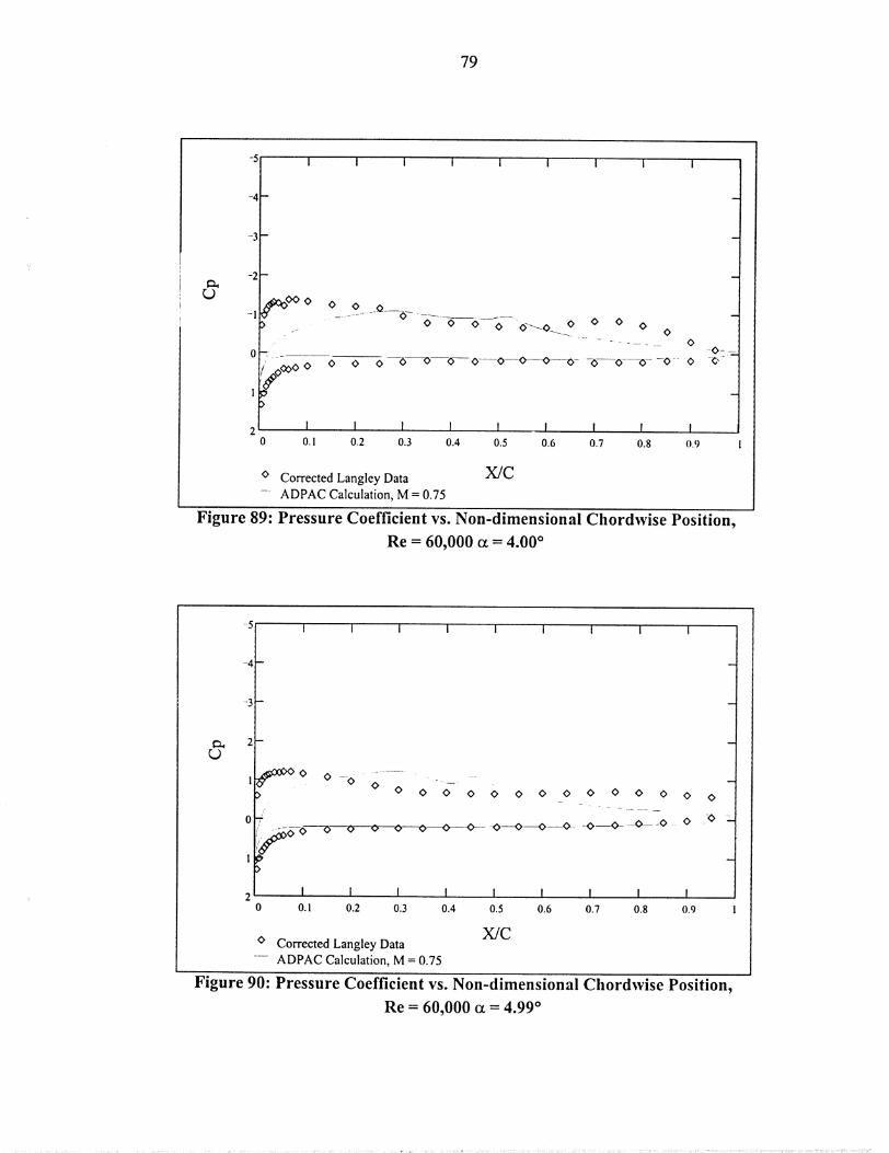
79

-5 I I i i I i i I I

-4

-3

-2

_<>oo ......?........°-_>-_ ....c--o--;_o--_.o___o....-, o_ <>o- O

0 ;'_ ...... ----- -O-

"-0_0 0 0_0----'0----0_---0- -0--0--0- --0-- 0 --00 0 00

2 I I I I I ! I ! !

0.1 0.2 0.3 0.4 0.5 0.6 0.7 0.8 0.9

O Corrected Langley Data X/C



Re = 60,000 tx = 4.00"

I I I i i i i i I

7>

/

"7

°--0 o o

o 0 0 0

0 0 0 0 o. 0 0 0 0 0 o o o_,

_.

0 _-0---0---0--0- --0--0--0---0 0 -0 --

, I I i I I I l I I

0 0.1 0.2 0.3 0.4 0.5 0.6 0.7 0.8 0.9



X/C


Re = 60,000 t_ = 4.99 °

80

-2

I I I _ I I I i I

_0> ..........-.... "0--_-00

>

[;

0 0 0 0 0 0 ....0 0 0 0 0 0

o---o-----6---o----o_o---o--o--o---o---o- -o....o ....o.--o

l I I I I I I I I

0 0.1 0.2 0.3 0,4 0.5 0.6 0.7 0.8 0.9



X/C

o o

o "-o-:-_


Re = 60,000 t_ = 6.01 °

-2

I I I I I I I I I

i __ 0 0 0 0 0 0 0 0 0-! --'-f .... - ........ 0

V ...."...._ - -0---0--_- -0

0 .....o-

I___oo o o o o o o

2L,. ! ! ! I I 1 ! ! !0 0.1 0.2 0.3 0.4 0,5 0.6 0.7 0.8 0,9


_- ADPAC Calculation, M = 0.75

X/C


Re = 60,000 t_ = 7.00 °

oo

_0o

o o

,<>o

o o

o o

0 oi

O_ 0

0 0

/

° !o

/o

o

o

-" " I ' 'I' I..... I .... |..... i ............

oo

o o

o

? o!

o

oj o

og

/

0

0 --"

0

o

0

o I o- o l o -

J , I 0

oP°̂°°_ J _::::::::::,...........-A'___

0

0

0

0

(-,,.

II

>.,,.o

o_O_

o 0

0om

o_

o

Im

o

oo_

0

E_o_

o

o_

Deml

_Do_eo

o

t_

t_

De

o

II

II

---Itji

g_II

_D_D

O

o

oo

o

oo

o

oo

_g0

z

_-go

o

Number of

Separated Points

Number of

Supersonic Points

to .1_

g

ii -

l-

_ I ......... g

to

oo

g

Log 10RMS Error

d,I

/J

/

-//

I

De

_DtJIee

¢3o

t_

_mle

o

II

II

--dLXl

II

O

o

g

g

N,-.,,

'-.I

__.

0

z

'-1

t_

g-Q

O

Number of

Separated Points

0 00 00 0

I0

0

Number of

Supersonic Points

....,

g

i

tti

g

Log 10RMS Error

I

Il

-IJ

ooIx9

Imme

t_kDO0ee

0"Q¢'D

t_

lame

oml

t_

II

II

...dL#I

g_II

",,4

O

0

--t

z

-'I O

Number of

Separated Points

l,d

Q0

1

I

,,

¢

(I:L

(?

_ 1i

J

(1

_______1______

Number of

Supersonic Points

o

............I!

..,,-

r

Log 10RMS Error

oo _, £.

f

t..¸

m

,,

.,

.,

...

..

ee

_,

_m

II

II

II

0

a"

z°

Number of

Separated Points

I

t1_

J ._

........... _ | ,,

oo

Number of

Supersonic Points

..... i .... ,

;. ; | ..............

Log 10RMS Error

oo

I

1 ,., i

ooL_

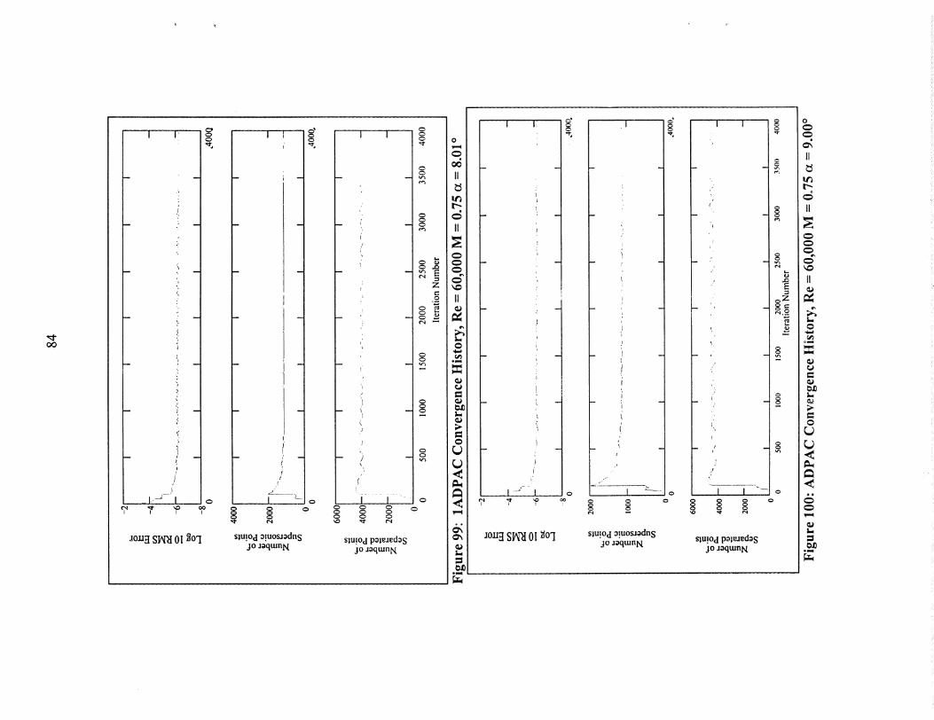
-a'-oo

I I ¸,' ¢_ IO

.I

... ._ ...

: I,

[ ',

t., t

(.,, _ ,,,p 0o _ g o

i0.I.I_[ S_ 0 [ _0"I slu't°d °!u°s't°dnsjo J0qmnN

m

I I

L

i

J

l-- i

]

f

0 0 0 00 0 0

slu!od poleaedosjo Joqtun N

1-

°_t/%t"q

x

¢...,

O t-0,2

eq --

o

odII

It3

i

II

_D

II

o

ella

_D

1,1_D

OL_L_<

o •

o_o_

t_J0ellm

I

J

t

.

O

oo

........ I :: I ....... i...... "--- o

i

I

L

r

I

i

nI

I'

,r

../.

o o

¢,,,i ,,-,

gL.¢J

E

oxo I::::

_.o_¢'3L..¢J

_0LI;:[ S_[_[ 0[ _°'I slu!od o.tuosJodnsjo aoqmn N

slu!od poleJedosjo Joqtun N

O

i

Ox

It

It%

II

o.,

_D

II¢.2

1,1O

ollm

_D_J01,1

L_L_.<

.<oe

_D

emll

85

Figure 101- Pressure Distribution for Re = 60,000 M - 0.45 cx= 8.01 °

Figure 102" Streamlines Over the Suction Surface of the Airfoil,

Re = 60,000 M = 0.45, _= 8.01 °

CHAPTER 6

Propeller Design and Analysis Using Two-Dimensional ADPAC Predictions

The designs in Chapter 4 using only the low speed Langley data neglected the

effects of compressibility. Even the Prandtl-Glauert compressibility corrections are

inadequate for the tip sections. To account for the compressibility effects, the

resulting lift and drag curves for each of the conditions listed in Table 3 were

incorporated into the strip theory design and analysis programs (Figures 49 through

52). Again, simple conditional statements were used to apply these predicted values

along the length of the blade.

The first design exercise was to see what effect elevated Mach numbers would

have on the propellers designed using only the Langley experimental data. Keeping

the number of blades, diameter, and Reynolds number distribution the same as was

used for the initial designs, new designs were made. The new twist, chord, and lift

coefficient distributions can be found in Figures 103 through 105.

Examination of the twist distribution still show a 'hook' near the tip. In these

designs, though, this 'hook' results from the degradation in performance as Mach

number is increased, rather than from the laminar stall found in the Langley data at

low angles of attack. Efficiencies of the three and four-bladed propellers using the

ADPAC predictions were 80.3% and 76.4%. These values are roughly 5% less than

the efficiencies predicted for the low speed designs using the low speed Langley data

alone.

86

87

To optimize the design, a lift coefficient distribution asymptotically reaching

the average maximum lift-to-drag ratio point along the blade was specified (Fig. 106).

This was done to increase the chordlengths of the inboard sections, as was seen to be

necessary in Chapter 4. The resulting propeller twist, chord, Reynolds number, and

relative Mach number distributions can be found in figures 107 through 110.

Efficiency for this propeller at design point was 85.1%. This propeller was

considered to be the final design.

The strip-theory analysis program was used to generate off-design propeller

performance predictions for the final design. Input to the analysis program includes

the propeller geometry, advance ratio, pitch angle, cruise Mach number, and altitude.

The program iterates to find the induced velocities and induced angle of attack. From

this information, the lift coefficient distribution along the blade can be found and

propeller thrust, power, and torque coefficients as well as efficiency can be calculated.

Among the many tests of programming integrity, performance calculated by the

design program should and did exactly match that calculated by the analysis program

at design point.

The off-design performance maps were created by changing the advance ratio

and pitch angle of the propeller. Variations of the propeller efficiency, thrust, power,

and torque coefficients for a range of pitch angles are shown in figures 111 through

114. At design point, the value of the advance ratio is 1.814 and the blade twist angle

at the 75% radial position is 42.52 ° .

88

Examinationof theoff-design performance curves for the propellers indicates

that there may be some merit to operating the propeller at a slightly higher pitch angle

than that at the design point. While maintaining the design advance ratio of 1.814,

increasing the pitch angle so that the angle at the 75% radial position is 45 °, a 25%

increase in thrust can be realized for a penalty of 5% in efficiency. Operating at this

point may be desirable if sufficient engine power is available. Increasing the pitch

setting past this point may not be recommended since the blade begins to stall when

the angle at the 75% radial station reaches 50 ° as shown in Figure 115. To decrease

the advance ratio while maintaining a constant cruise velocity may not yield the

predicted increase in thrust since as tip speeds increase, shock waves will affect a

larger portion of the blade degrading perfo_ance. A comparison of the design point

conditions and those for this high thrust case can be found in Table 4. Actual

performance for both cases will vary from the predicted values as the blades twist in

operation. A structural analysis would need to be conducted to understand the

propeller's performance more fully°

89

Table4. Comparisonof theDesignPointandMaximumThrustPoint

Efficiency

DesignPointPitchAngleat 75%R=

42.52°

0.8509

Maximum Thrust Point

Pitch Angle at 75%R =

45.00 °

0.8107

Thrust Coefficient 0.1411 0.1780

Power Coefficient 0.3007 0.3983

Torque Coefficient 0.0479 0.0634

Thrust

Power

Torque

450.9 N

(101.3 lbs)

63.4 kW

(85 hp)

703.7 N-m

(519.0 ft-lbs)

1.814Advance Ratio

569.0 N

(127.9 lbs)

83.9 kW

(112.6 hp)

932.1 N-m

(687.5 ft-lbs)

1.814

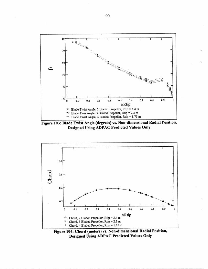
90

8O

7O

6O

5O

4O

30'

i I I

.-...

-...\

I I I I I I

I I I I I I I0 0.1 0.2 0.3 0.4 0.'i 0.6 0.7

r/Rtip

-o- Blade Twist Angle, 2 Bladed Propeller, Rtip - 3.4 m

_ Blade Twis Angle, 3 Bladed Propeller, Rtip = 2.3 m

-+ Blade Twist Angle, 4 Bladed Propeller, Rtip = 1.75 m

! I0.8 0.9 l

Figure 103: Blade Twist Angle (degrees) vs. Non-dimensional Radial Position,

Designed Using ADPAC Predicted Values Only

I-iO

r..)

0.8

0.6

0.4

0.2

I I I I I i I I i

-_- Chord, 2 Blade<_ Propeller, Rtip = 3.4 m

_ Chord, 3 Bladed Propeller, Rtip = 2.3 m

-+- Chord, 4 Bladed Propeller, Rtip = 1.75 m

! I I I

0.3 0.4 0.5 0.6

r/Rtip

I !0.7 0.8 0.9

Figure 104: Chord (meters) vs. Non-dimensional Radial Position,


\

\.\ ,, ,\

-.,

..

- III

u.

!.

', ,

_._-__

R', I

J,u0!0K40OD _,2!'1

¢:h _c,i,-;"._ II II II

d

O O O

888

o ,._t

0em

em

o

m

@om

ellll

@

em

E@

ellll

Ii

em

o

OO

O

O

¢.qo

o

O

f_

oelm

em

O

m

em

¢d

L_

em

em

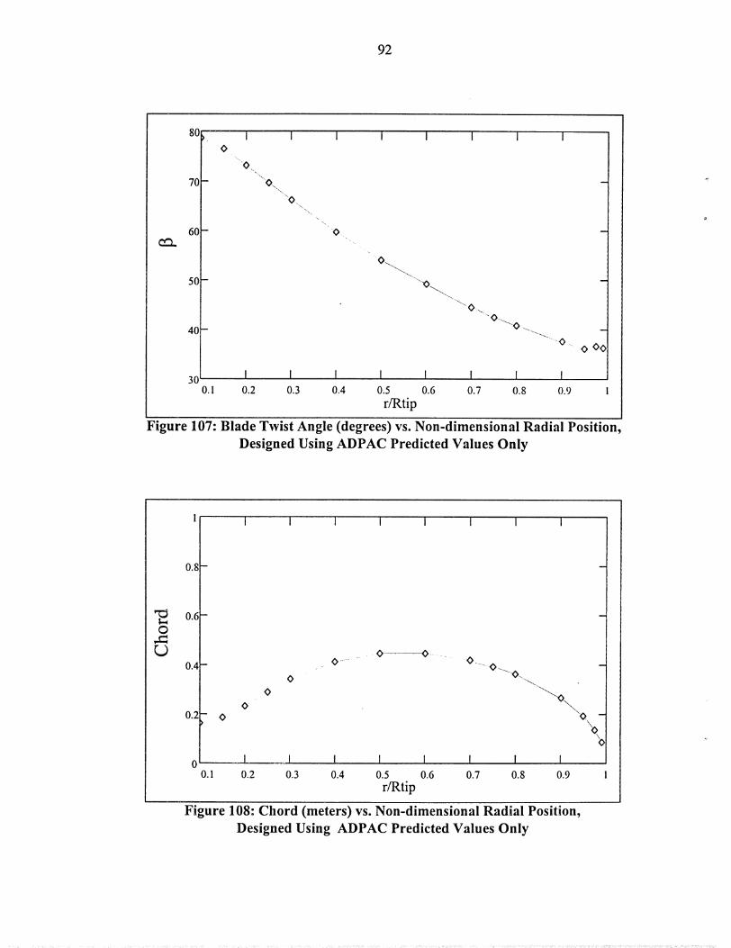
92

80

70

60

50

40

<>I i I I I I I I

\O\

""O-

" O L.,_.

! I30 I ! ! ! I !0.1 0.2 0.3 0.4 0.5 0.6 0.7 0.8 0.9

r/Rtip

Figure 107: Blade Twist Angle (degrees) vs. Non-dimensional Radial Position,


O

L)

0.8

0.6

0.4

0.2 - <>

0.1

I I I I I I I i

O-- O ........O ........... O .....

I .... ! ! ! I I !0.2 0.3 0.4 0.5 0.6 0.7 0.8

r/Rtip

I0.9 I

Figure 108: Chord (meters) vs. Non-dimensional Radial Position,


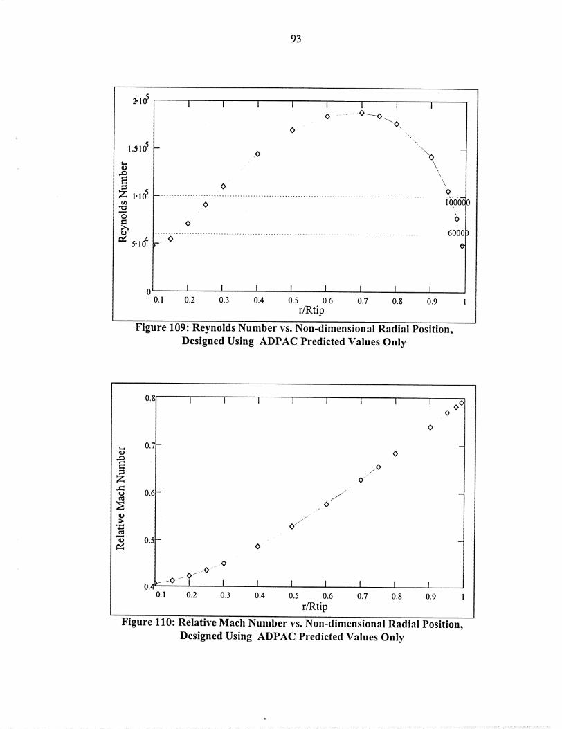
93

,.Q

1.51050

.

I I i

\.

0

1.105

o0

_:_ 5.104 0

I ! I ! I ! ! I0.2 0.3 0.4 0.5 0.6 0.7 0.8 0.9

r/Rtip

0.|

\\

\

\t>10000

O

6000

Figure 109" Reynolds Number vs. Non-dimensional Radial Position,


2:

0.8

0.7

0.6

0.5

0.4

I i I I i i I 1

rio_O _

A

,_I-O .... _J I

0.l 0.2 0.3

O

O

/

fJ

I I I I ! !0.4 0.5 0.6 0.7 0.8 0.9

r/Rtip

m

0 o0

Figure 110" Relative Mach Number vs. Non-dimensional Radial Position,


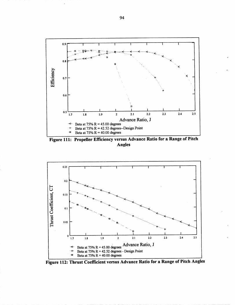
94

¢j

0.9

0.8

0.7

0.6

0.5

I I I I I I I

1.7

l I I1.8 1.9 2

"'" ''",.....,

\,

I I2.1 2.2

Advance Ratio, JBeta at 75% R = 45.00 degrees

_' Beta at 75% R = 42.52 degrees--Design Point

-_ Beta at 75% R = 40.00 degrees

_<

K

I I2.3 2.4 2.5

Figure 111" Propeller Efficiency versus Advance Ratio for a Range of Pitch

Angles

0.25

0.2

"_ 0.15_D

0.!O

4--1r_

d_ 0.05

[..,

I I I I I I I

I I I2.2 2.3 2.4 2.5

-'<- Beta at 75% R = 45.00 degrees Advance Ratio, J

÷ Beta at 75% R = 42.52 degrees- Design Point

-_ Beta at 75% R = 40°00 degrees

Figure 112: Thrust Coefficient versus Advance Ratio for a Range of Pitch Ang es

95

L_4_

.p,q

O

O@

L_

O

0.5

04

0.3

0.2

0.1

I I I I I I I

T:_L. -.

-...

"U

I I I I I

.7 1.8 19 2 2.1 2.2

Advance Ratio, J--x- Beta at 75% R = 45.00 degrees

+ Beta at75% R = 42.52 degrees-Design Point

-o- Beta at 75% R. = 40.00 degrees

! 1

2.3 2.4 2.5

Figure 113: Power Coefficient versus Advance Ratio for a Range of Pitch Angles

0.08

0 /0.06

o_

0

0.0400

rjtD

0.02

I I i I I I I

-_ 'B°--.. "4-. -....

"B

"'0_.

--....

"13

"-x...-...g...

"'._

1.7

I I I I I I I1.8 1.9 2 2.1 2.2 2.3 2.4 2.5

Advance Ratio, JBeta at 75% R. = 45.00 degrees

÷ Beta at 75% R = 42,52 degrees - Design Point

-_ Beta at 75% R = 40.00 degrees

Figure 114: Torque Coefficient versus Advance Ratio for a Range of Pitch

Angles

96

o _,..I

O

O

• _,,MI

1.5 I I I I

s

/o

.....' - - o

/K ...p'" X

/' ..

,.

_. I I k0.5 I

_,- --O - <)-- - - " -0 - <_

, / |

' I' I -

X ,K--_

/.---._'" I I

X ..... -I,-" .... I

.- _.--'I" .... I' 'Ir_o,

11 _ _ ---.a-_D .... ---B---I_|

I' I

/ I

1.5 2 2.5

Radius, meters-_- Beta at 75% R - 45.00 degrees÷" Beta at 75% R = 42.52 degrees - Design Point

-a- Beta at 75% R = 40.00 degrees

-_" Beta at 75% R = 50.00 degrees

Figure 115: Lift Coefficient Distributions for a Range of Pitch Angles

CHAPTER 7

ADPAC Three-Dimensional Performance Calculations

A three-dimensional model of the propeller was made from the twist and

chord distributions (Fig. 107-108) calculated using Adkins' and Liebeck's strip theory

design methods (Ref. 5). Views of the propeller's solid surfaces can be seen in

Figures 116 and 117. The computational mesh of the flowfield around the propeller

extends one radius upstream of the propeller, one radius downstream, and one radius

radially outward from the blade tip, The entire mesh contains 4,157,138 grid points.

The hub surface was modelled as a simple cylinder. The blade suction and pressure

surfaces were established as "no-slip" surfaces while the cylindrical hub was

established as a "slip" surface. Total temperature and total pressure were fixed on the

vertical inlet plane, and freestream static pressure was fixed at the vertical exit plane.

The freestream Mach number was fixed on the cylindrical outer boundary of the

computational grid.

A program called TCGRID written by Roderick V. Chima (Ref. 14) was used

to create a fine "C" grid around one propeller blade as well as a somewhat coarser

"H" grid farther upstream of the blade. Since TCGRID was originally intended to

generate meshes for turbomachinery blading, it was a challenge to create an

appropriate mesh for such a large blade with this program. The two grid blocks made

with TCGRID were modified so that the final mesh consisted of ten separate grid

blocks. As shown in Figure 118, the fine "C" grid block was broken into four

97

98

separateblocks (Blocks 1-4),andthecoarseinlet block is shownin yellow asBlock

5. The fine meshwas retainedfor Block 1 closestto the blade,while themeshwas

coarsenedby eliminating everyothergrid line from the original fine meshto yield

Blocks 2 through4. The coarsemeshwasbrokenat the comersof the "C" grid to

avoid possibleproblemswithin ADPAC concemingstretchingratios,or the relative

sizeof neighboringcomputationalcells. Figure 119is aview forward looking aft of

thecomputationaldomainsurroundingoneof thethreepropellerblades. Figures120 •

through122showtheportion of the computationalmeshnearthe inlet block region,

near the blade hub, and near the exit region, respectively. SeparateFORTRAN

programswere written to extend the mesh radially outwards creating Blocks 6

through10(Fig. 123).

Therearemany featureswhich aredesiredof a computationalmesh_some

for physical reasonsand some to comply with the ADPAC program format.

Physically,thereagainshouldbeenoughgrid pointspackedcloseto thebladesurface

sothat theboundarylayercanbe resolved.Thegrid shouldalsoextendwell into the

free streamaheadof the blade,behind the blade,and radially outward. It is also

recommendedthat thegridlinesfollow thetrailing edgeangleof thebladesectionsso

that separationandanyvorticesthat maybe shedcanbeseen. The challengewhen

creatinga meshis meetingall theserequirementswhile keepingthe numberof grid

points to a minimum to reducecomputationaltime. Practically, the upstreamand

downstreamextentsof the meshweresacrificedin orderto addgrid points closerto

99

the blade surface. Even so, the three-dimensional mesh is much coarser than the two-

dimensional meshes seen earlier. Values for y+ of the first grid line above the blade

surface at approximately the quarter chord location were 2.266 for the section at

r/Rtip = 0.406, 2.692 for the section at r/Rtip = 0.666, and 3.671 at r/Rtip = 0.905.

For a mesh to be suitable for an ADPAC three-dimensional calculation,

stretching ratios for the cells should be around 1.3. TCGRID did not contain input

parameters to vary stretching ratios directly, so this requirement was met by adding

grid points until the stretching ratios near the tip were within acceptable bounds.

ADPAC uses a multigrid method to speed convergence. This technique generates

intermediate solutions by coarsening the mesh by eliminating grid points. Three

levels of multigrid are recommended and can be achieved if the number of cells in

each direction for each block are divisible by four. Coordinates for the leading edge

and trailing edge of the blade must also meet this criterion if the multigrid technique

is to be used. If an "H" grid is used for an inlet block, the upstream edge of the "C"

grid must be square and must not overlap the inlet block cells. Finally, coordinates of

all grid blocks must be ordered to form a left-handed coordinate system.

ADPAC was used to calculate the steady state viscous flow over the rotating

propeller blade at the design conditions. The convergence history plots are shown in

Figure 124. After over 2500 iterations, the solution was considered to be converged

because the RMS error had decreased by three orders of magnitude and the number of

separated points was constant. Figure 125 shows three blade sections near the hub,

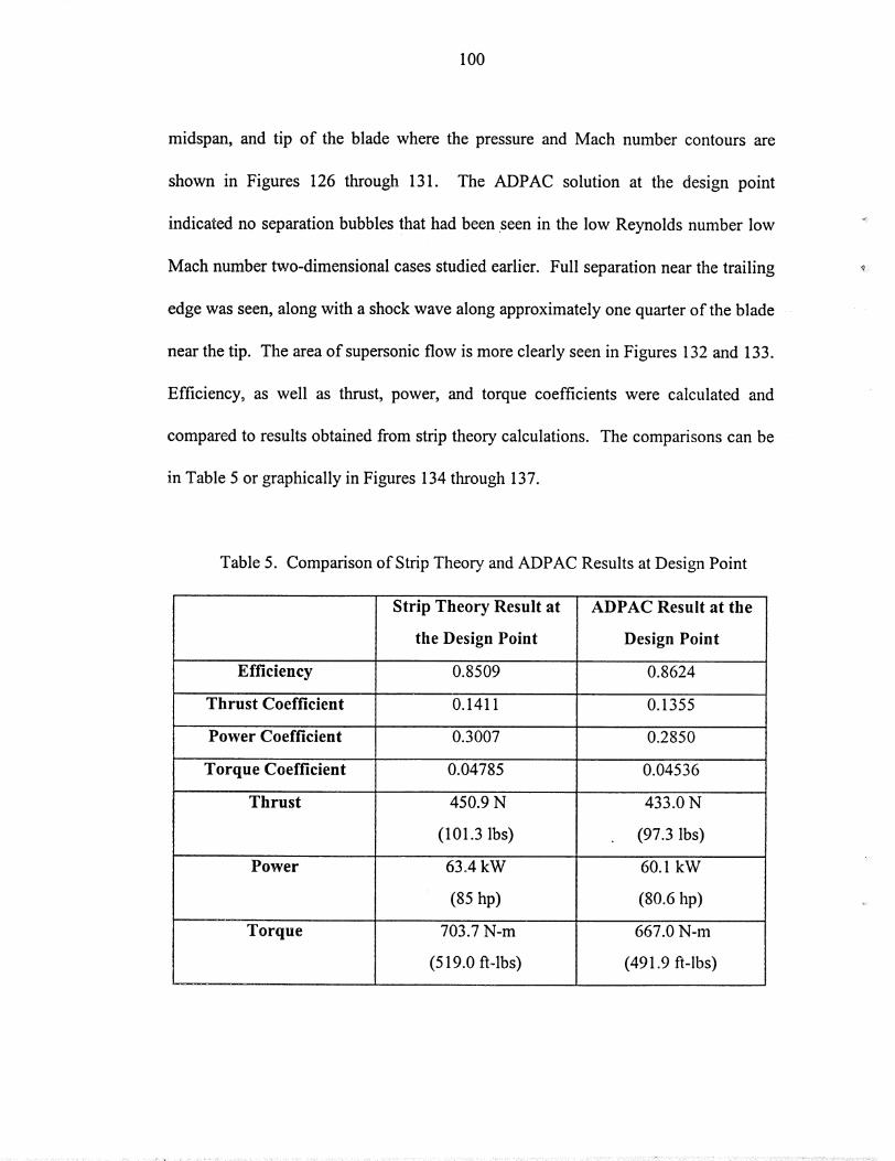
100

midspan,and tip of the blade where the pressure and Mach number contours are

shown in Figures 126 through 131. The ADPAC solution at the design point

indicated no separation bubbles that had been seen in the low Reynolds number low

Mach number two-dimensional cases studied earlier. Full separation near the trailing

edge was seen, along with a shock wave along approximately one quarter of the blade ......

near the tip. The area of supersonic flow is more clearly seen in Figures 132 and 133.

Efficiency, as well as thrust, power, and torque coefficients were calculated and

compared to results obtained from strip theory calculations. The comparisons can be

in Table 5 or graphically in Figures 134 through 137.

Table 5. Comparison of Strip Theow and ADPAC Results at Design Point

Efficiency

Thrust Coefficient

Power Coefficient

Torque Coefficient

Thrust

Power

Torque

Strip Theory Result at

the Design Point

0.8509

0.1411

0.3007

0.04785

450.9 N

(101.3 lbs)

63.4 kW

(85 hp)

703.7 N-m

(519.0 ft-lbs)

ADPAC Result at the

Design Point

0.8624

0.1355

0.2850

0.04536

433.0 N

(97.3 lbs)

60.1 kW

(80.6 hp)

667.0 N-m

(491.9 fi-lbs)

101

power, and torque coefficients were approximately 5% lower. This difference can be

attributed to several factors. First, because of the simplistic application of the two-

dimensional low Reynolds number transonic predictions, the strip theory design did

not account for the shock from r/Rtip of approximately 0.75 to 0.90. Secondly, the

three-dimensional mesh was considerably less dense than the two-dimensional

meshes and may be below the value for which the solution is independent of the

number of grid points. Finally, the tip vortices as shown in Figure 138, were not

taken into account in the strip theory design and analysis programs. The tip vortex

from one blade and the blade wake can also be seen in the Mach number distribution

at the exit of the computational domain shown in Figure 139.

102

Figure 116: The Three-Bladed Propeller and Extended Hub Surface, Side View

Figure 117: Front View of Three-Bladed Propeller

103

BIock t

Block 2Block 3

Block 4

Figure 118: Computational Mesh Blocks and Solid Surfaces, Axial View

i¸¸

Figure 119: Forward Looking Aft View of Propeller Blade and ComputationalMesh Blocks

104

Figure 120: Magnified View of Inlet Block Region

Figure 121" Magnified View of Blade Region

105

Figure 122- Magnified View of Trailing Edge Region

Figure 123: View of Computational Mesh Upstream and Above the Blade Tiw--

Forward Looking Aft

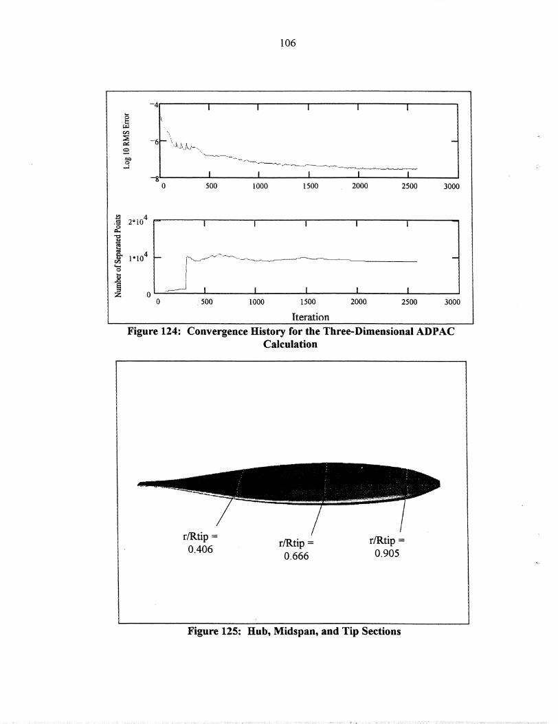
106

O,--1

-4

-{

-8'

I I I i I

, I I0 500 1000

I I I1500 2000 2500 3000

._ 2-i0 4O

_ 1.104r_

o

z 0

I I I i I

..-..

,.,-,, _",,-,,.,,.,__ ._,__"'_ "'_--._...-..._.,___

0 5O0 1000

I I I1500 2000 2500

Iteration

3OO0

Figure 124: Convergence History for the Three-Dimensional ADPACCalculation

!

r/Rtip = r/Rtip = r/Rtip =0.406 0.666 0.905

Figure 125" Hub, Midspan, and Tip Sections

107

Pressure Ratio, Ps/Pt

1.2500

0.7$00

. ,9.2500

i

Figure 126: Pressure Ratio Contours for r/Rtip = 0.406

\

Math Number \_l,

/

Figure 127- Mach Number Contours for r/Rtip - 0.0406

108

i

/

/,- . _. _ ./

!/ / .......l_mre Ralio, PI/Pt

<!/ /

i .\_-J ,: \ ,

.! \. ./

:: ",. /

Figure 128: Pressure Ratio Contours for r/Rtip = 0.666

Maeh Number

1=5000

0.7500

0.0000

....k.

/Figure 129: Mach Number Contours for r/Rtip = 0.666

Oi,,,,,,-I

C_C_

II

z,,

r_

0

C_

E

c_

ee

N)em

110

Figure 132: Suction Surface Pressure Distribution

Figure 133: Mach Number Distribution Over the Suction Side of the Blade

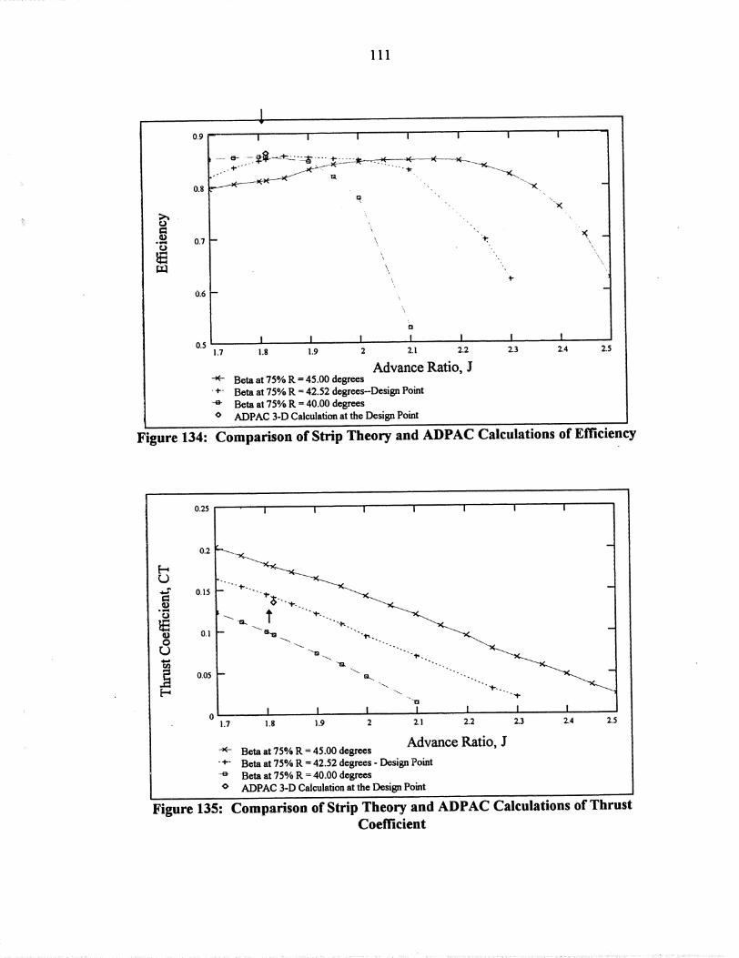
III

0.9

0.8

o

o., _,,=a

[.T-1

0.7

0.6

0.5

\

'.\

\

'\

,\

I I I I

I.g !.9 2 2.1

I, ,,

2.2

Advance Ratio, J-_- Beta at 75% R = 45.00 degrees

+ Beta at 75% R = 42.52 degrees-Design Point

Beta at 75% R = 40.00 degrees

o ADPAC 3-D Calculation at the Design Point

I I I

_-..,--,-...._.....

4"

\

I I2.3 2.4 2.5

Figure 134: Comparison of Strip Theory and ADPAC Calculations of Efficiency

aJ®p=q

QJO

4--t

0.25

0.2

0.15

0.1

0.05

I I I I I I I

I I I1.7 1.8 i.9 2

Advance Ratio, JBeta at 75% R = 45.00 degrees

+ Beta at 75% R = 42.52 degrees - Design Point

-_ Beta at 75% R = 40°00 degrees


Figure 135: Comparison of Strip Theory and ADPAC Calculations of ThrustCoefficient

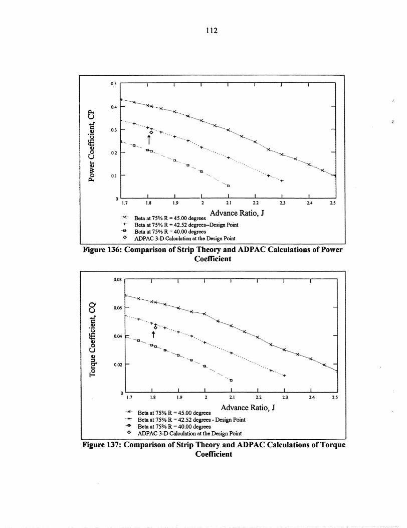
112

r,..)

0

r,..)

0

0.5

0.4

0.3

0.2

0.I

I I I I I .i i

_-rl

1.7

I I I I I I !

1.8 !.9 2 2.1 2.2 2.3 2.4 2.5

Advance Ratio, J--'<- Beta at 75% R = 45.00 degrees

_ Beta at 75% R = 42.52 degrees-Design Point

-o Beta at 75% R = 40.00 degrees


Figure 136: Comparison of Strip Theory and ADPAC Calculations of PowerCoefficient

CY

4--t

O_.vm

O

0.08

0.06

0.04

0.02

I i i I i I I

==. _

B..

13

I I I I

1.7 1.8 1.9 2 2.1

I ! , !

2.2 2.3 2.4

Advance Ratio, J-_ Beta at 75% R = 45.00 degrees

t Beta at 75% R = 42.52 degrees - Design Point

-e- Beta at 75% R = 40.00 degrees


iI

!-,i

2.5

Figure 137: Comparison of Strip Theory and ADPAC Calculations of Torque

Coefficient

111

0.9

0.8

I I ! I

o

oI,,_

o

Er.l.l

0.7

0.6

0.5

Q,

:\

\

\i

I I I I

1.8 1.9 2 2.1

-_- Beta at 75% R = 45.00 degrees

o

I2.2

Advance Ratio, J

Beta at 75% R = 42.52 degrees-Design Point

Beta at 75% R = 40.00 degrees

ADPAC 3-D Calculation at the Design Point

I I I

•"'" "4- _, -• \

\

4"

I I2.3 2.4 2.5

Figure 134: Comparison of Strip Theory and ADPAC Calculations of Efficiency

0.25

0.2

0.15

O

E0.1

0

rj)

0.05

I I I I I i i

Advance Ratio, J-3<-- Beta at 75% R = 45.00 degrees

4- Beta at 75% R = 42.52 degrees- Design Point

-o Beta at 75% R = 40.00 degrees


Figure 135: Comparison of Strip Theory and ADPAC Calculations of ThrustCoefficient

112

0o

g.,

o

0.5

0.4

0.3

0.2

O.l

I I I I I .I I

I ! I I I I !1.7 1.8 1.9 2 2.1 2.2 2.3 2.4

Advance Ratio, J-'_ Beta at 75% R = 45.00 degrees

_ Beta at 75% R = 42.52 degrees-Design Point-o Beta at 75% R = 40.00 degreeso ADPAC 3-D Calculation at the Design Point

2.5

Figure 136" Comparison of Strip Theory and ADPAC Calculations of Power

Coefficient

CY

4-a

Oo

0.08

0.06

0.04

0.02

I I i f' I I I

I I I I ! I , I1.7 1.8 1.9 2 2.1 2.2 2.3 2.4 2.5

Advance Ratio, J-_ Beta at 75% R = 45.00 degrees

_' Beta at 75% R = 42.52 degrees - Design Point

-e- Beta at 75% R = 40.00 degrees


Figure 137" Comparison of Strip Theory and ADPAC Calculations of TorqueCoefficient

113

........ :.........

Figure 138: Tip Vortex Streamlines

Exit Plane Math Number

O.3OOO O.4OOO O..._H)O

Figure 139: Pressure Distribution at the Exit Plane of the ComputationalDomain

CHAPTER 8--CONCLUSION

Comparison of the strip theory design and analysis results with those from

ADPAC, a numerical Navier-Stokes analysis code, sheds light on the strengths and

weaknesses of both techniques. Propeller efficiency predicted by ADPAC was

within 1.5% of that calculated with the strip theory methods at the design point while

ADPAC predictions of thrust, power, and torque coefficients were approximately 5%

lower than the strip theory results.

The main advantage to the strip theory design and analysis methods is speed.

Since design is an iterative process, the designer must be able to change conditions

easily and determine the propeller's geometry quickly and Adkins' and Liebeck's

procedures prove to be a useful tool. Results from strip theory analyses can be

obtained quickly as well, a necessity when calculating performance at many off-

design conditions in order to create a propeller map. Despite the simplifying

assumptions made, reasonable accuracy was achieved with Adkins' and Liebeck's

strip theory methods.

The main advantages of using ADPAC was the elimination of simplifying

assumptions required to make the performance calculation and the visualization of

results. Shocks and tip vortices ignored in the strip theory analysis were clearly seen

in viewing the ADPAC results. However, the improvement in the analysis required a

substantial amount of time to Ieam how to run the code, to create appropriate meshes,

and to post-process the output files. This time is in addition to that required to

114

115

actually run the calculation. Thethree-dimensionalmeshconsumeda greatamount

of time sinceapproximately22 hourswere neededto complete100 iterationson a

dedicatedworkstationwith anR8000processor.

In conclusion,thefusion of two dimensional strip theory design and analysis

methods with ADPAC, a three-dimensional Navier-Stokes yielded a good first-

generation propeller design for a vehicle capable of subsonic flight in Earth's

stratosphere. Lift and drag coefficients for the Eppler 387 at low Reynolds number

transonic conditions were generated with ADPAC since experimental results were

unavailable for this regime. Examination of the three-dimensional results showed

that the Eppler 387 was not a suitable airfoil for at least the tip sections of the

propeller because of the shock waves seen on the suction surface of the relatively

thick outboard sections. Improvements can be made to this design by combining two-

dimensional airfoil ADPAC results for other airfoils into the strip theory design and

analysis methods (if experimental data is unavailable), making a full three-

dimensional prediction only after several design iterations are made.

REFERENCES

[1 ] ERAST Leadership Team. 1996. A Review of Remotely Piloted Aircraft (RPA)

Technology Required for High Altitude Civil Sciences Missions.

Washington, D.C.: NASA, Office of Aeronautics (Code R), Office of Mission

to Planet Earth (Code Y). Photocopied.

[2] Adkins, C.N. and R.H. Liebeck. 1983. Design of Optimum Propellers. New York"

American Instintue of Aeronautics and Astronautics. AIAA-83-0190.

[3] Mueller, To J. 1985. Low Reynolds Number Vehicles. Neuilly-Sur-Seine, France:

Advisory Group for Aerospace Research and Development. NTIS,

AGARDograph No. 288.

[4] Pauley, LoL. and P. Moin and WoC. Reynolds. 1989. The Instability of Two-

Dimensional Laminar Separation. In Low Reynolds Number Aerodynamics:

Proceedings of the Conference in Notre Dame, Indiana. June 5-7, 1989 by

Springer-Verlag, 82-92. New York: Springer-Verlag.

[5] McGhee, R.J. and B.J. Walker and B.F. Millard. 1988. Experimental Results for

the Eppler 387 Airfoil at Low Reynolds Numbers in the Langley Low-

Turbulence Pressure Tunnel. Washington, D.C. NASA TM-4062.

[6] Drela, M.1989. XFOIL: An Analysis and Desing System for Low Reynolds

Number Airfoils. In Low Reynolds Number Aerodynamics: Proceedings of

the Conference in Notre Dame, Indiana, June 5-7. 1989. By Springer-

Verlag. 1-12. New York" Springer-Verlag

[7] Drela, M. 1992. Transonic Low-Reyonlds Number Airfoils. Journal of Aircraft.

Volo 29 No. 6 (Nov.-Deco) ° 1106-1113.

[8] Coiro, D.Po and CodeNicola. 1989. Prediction of Aerodynamic Performance of

Airfoils in Low Reynolds Number Flows. In Low Reynolds Number

Aerodynamics: Proceedings of the Conference in Notre Dame, Indiana. June

5-7, 1989. By Springer-Verlag. 13-23, New York: Springer-Verlag.

[9] Hall, E.Jo and D.A. Top and R.A. Delaney. Task 7-ADPA C Users

Manual.Cleveland: NASA Lewis Research Center, NASA CR-195472.

[ 10] Schlichting, H. 1960. Boundary Layer Theory. New York: McGraw-Hill.

116

117

[11] Glauert,H. 1926.The Elements of Aerofoil and Airscrew Theory, Cambridge"

The University Press.

[ 12] McCormick, B.W. 1979. Aerodynamics, Aeronautics, and Flight Mechanics,

New York: John Wiley and Sons.

[ 13] Anderson, J.D. 1989. Introduction to Flight. New York: McGraw-Hill Book

Company.

[ 14] Chima, R.V. 1990. TCGRID. Cleveland: NASA Lewis Research Center.

REPORT DOCUMENTATION PAGE ! FormApprovedOMB No. 0 704-0188

Public reporting burden for this collection of information is estimated to average 1 hour per response, including the time for reviewing instructions, searching existing data sources,gathering and maintaining the data needed, and completing and reviewing the collection of information. Send comments regarding this burden estimate or any other aspect of thiscollection of information, including suggestions for reducin_ this burden, to Washington Headquarters Services, Directorate for Information Operations and Reports, 1215 JeffersonDavis Highway, Suite 1204, Arlington, VA 22202-4302, and to the Office of Management and Budget, Paperwork Reduction Project (0704-0188), Washington, DC 20503.

1. AGENCY USE ONLY (Leave blank)

4. TITLE AND SUBTITLE

2. REPORT DATE

February 1998

3. REPORT TYPE AND DATES COVERED

Technical Memorandum

5. FUNDING I_IUMBERS

Design and Performance Calculations of a Propeller for Very High Altitude Flight

6. AUTHOR(S)

L. Danielle Koch

7. PERFORMING ORGANIZATION NAME(S) AND ADDRESS(ES)

National Aeronautics and Space Administration

Lewis Research Center

Cleveland, Ohio 44135-3191

9. SPONSORING/MONITORING AGENCY NAME(S) AND ADDRESS(ES)

National Aeronautics and Space Administration

Washington, DC 20546-0001

WU-529-10-I 3--00

8. PERFORMING ORGANIZATIONREPORT NUMBER

E-11102

10. SPONSORING/MONITORING

AGENCY REPORT NUMBER

NASA TMm1998-206637

11. SUPPLEMENTARY NOTES

This report was submitted as a thesis in partial fulfillment of the requirements for the degree of Masters of Science in

Engineering to Case Western Reserve University, Cleveland, Ohio, January 1998. Responsible person, L. Danielle Koch,

organization code 7565, (216) 433-5656.

12a. DISTRIBUTION/AVAILABILITY STATEMENT

Unclassified- Unlimited

Subject Categories: 02 and 07 Distribution: Nonstandard

12b. DISTRIBUTION CODE

14. SUBJECT TERMS

Propeller; High-altitude; Low Reynolds number aerodynamics; ADPAC

17. SECURITY CLASSIFICATION

OF REPORT

Unclassified

NSN 754_)-01-280-5500

18. SECURITY CLASSIIT:ICATIONOF THIS PAGE

Unclassifiedm

19. SECURITY CLASSIFICATION

OF ABSTRACT

Unclassified

15. NUMBER OF PAGES

]3016. PRICE CODE

A0720. LIMITATION OF ABSTRACT

Standard Form 298 (Rev. 2-89)

Prescribed by ANSI Std. Z39-18298-102

This publication is available from the NASA Center for AeroSpace Information, (301) 621--0390.

13. ABSTRACT (Maximum 200 words)

Reported here is a design study of a propeller for a vehicle capable of subsonic flight in Earth's stratosphere. All propellers presented

were required to absorb 63.4 kW (85 hp) at 25.9 km (85,000 ft) while aircraft cruise velocity was maintained at Mach 0.40. To produce

the final design, classic momentum and blade-element theories were combined with two and three-dimensional results from the

Advanced Ducted Propfan Analysis Code (ADPAC), a numerical Navier-Stokes analysis code. The Eppler 387 airfoil was used for each

of the constant section propeller designs compared. Experimental data from the Langley Low-Turbulence Pressure Tunnel was used in

the strip theory design and analysis programs written. The experimental data was also used to validate ADPAC at a Reynolds numbers of

60,000 and a Mach number of 0.20. Experimental and calculated surface pressure coefficients are compared for a range of angles of

attack. Since low Reynolds number transonic experimental data was unavailable, ADPAC was used to generate two-dimensional section

performance predictions for Reynolds numbers of 60,000 and 100,000 and Mach numbers ranging from 0.45 to 0.75. Surface pressure

coefficients are presented for selected angles of attack, in addition to the variation of lift and drag coefficients at each flow condition. A

three-dimensional model of the final design was made which ADPAC used to calculated propeller performance. ADPAC performance

predictions were compared with strip-theory calculations at design point. Propeller efficiency predicted by ADPAC was within 1.5% of

that calculated by strip theory methods, although ADPAC predictions of thrust, power, and torque coefficients were approximately 5%

lower than the strip theory results. Simplifying assumptions made in the strip theo_'y account for the differences seen.

Documents

Design and Performance Calculations of a Propeller for Very High Altitude Flight