Design and optimisation ofelectrocoagulation for use in

wastewater treatment.

Master’s Thesis

Silas A. C. Duus

Aalborg UniversityDepartment of Chemistry and Bioscience

Fredrik Bajers Vej 7HDK-9220 Aalborg Ø

Master studentDepartment of Chemistryand BioscienceFredrik Bajers Vej 7H9220 Aalborg Øhttp://www.bio.aau.dk

Titel:Design and optimisation of electro-coagulation for use in wastewatertreatment

Semester:3rd and 4th semester

Semestertema:Coagulation of wastewater

Project period:02.09.19 - 4.06.20

ECTS:60

Vejleder:Mads Koustrup Jørgensen

Project gruppeSeparationsgruppen

Master student:Silas Alf Christian Duus

Oplag: 1Antal sider: XXX siderAppendix: XXXBilag: Zip file

Abstract:

This project investigates the build of anelectrocoagulation cell, using a fixed cur-rent density, concentration, electrode setsand flow rate. The cell was generated inCOMSOL multiphysics 5.5, to simulate thefluid dynamics through the cell to investi-gate the turbulent velocities encounteredby the array of electrodes. Further morethe influence of the potential needed to runan electrocoagulation process will be in-vestigated using Nernst equation and thestandard reduction potentials for iron elec-trodes.

Preface 1The project ’Design and optimisation of electrocoagulation for use in wastewater treatment’was written by Silas A. C. Duus at the Department of Chemistry and Bioscience at AalborgUniversity during the 3rd and 4th semester (M.Sc) in Chemical engineering.

I would like to thank Mads Koustrup Jørgensen for supervising the project, interestingcollaboration, valuable inputs and guidance through the project.

References are listed as [number] after order of appearance at the end of the report. Thereport is split into 8 chapters. Additional pictures, schematics, calculations and data canbe found in the enclosed additional folder.

3

Contents

Chapter 1 Preface 3

Chapter 2 Abbreviations list 5

Chapter 3 Introduction 73.0.1 Treatment of waste water . . . . . . . . . . . . . . . . . . . . . . . . 73.0.2 Coagulation . . . . . . . . . . . . . . . . . . . . . . . . . . . . . . . . 9

3.1 Problem statement . . . . . . . . . . . . . . . . . . . . . . . . . . . . . . . . 103.2 Approach . . . . . . . . . . . . . . . . . . . . . . . . . . . . . . . . . . . . . 10

Chapter 4 Theory 114.1 Electrochemistry with sacrificial electrodes . . . . . . . . . . . . . . . . . . . 114.2 Concentration, ohmic potential and overpotential for electrolytic cells . . . . 124.3 Current and Current Density . . . . . . . . . . . . . . . . . . . . . . . . . . 134.4 Reactor settings and configurations . . . . . . . . . . . . . . . . . . . . . . . 164.5 Circuit . . . . . . . . . . . . . . . . . . . . . . . . . . . . . . . . . . . . . . . 184.6 Electrocoagulation process limits . . . . . . . . . . . . . . . . . . . . . . . . 19

4.6.1 Degradation of electrode . . . . . . . . . . . . . . . . . . . . . . . . . 194.6.2 Alternating and Direct Current . . . . . . . . . . . . . . . . . . . . . 194.6.3 Mass transport limit . . . . . . . . . . . . . . . . . . . . . . . . . . . 19

4.7 COMSOL . . . . . . . . . . . . . . . . . . . . . . . . . . . . . . . . . . . . . 19

Chapter 5 Experimental setups 215.1 COMSOL - Cell building . . . . . . . . . . . . . . . . . . . . . . . . . . . . . 21

Chapter 6 Results 256.1 Cell design . . . . . . . . . . . . . . . . . . . . . . . . . . . . . . . . . . . . 256.2 COMSOL simulations . . . . . . . . . . . . . . . . . . . . . . . . . . . . . . 27

6.2.1 laminar . . . . . . . . . . . . . . . . . . . . . . . . . . . . . . . . . . 276.2.2 turbulent . . . . . . . . . . . . . . . . . . . . . . . . . . . . . . . . . 28

Chapter 7 Discussion 317.1 Discussion . . . . . . . . . . . . . . . . . . . . . . . . . . . . . . . . . . . . . 31

7.1.1 COMSOL . . . . . . . . . . . . . . . . . . . . . . . . . . . . . . . . . 31

Chapter 8 Conclusion 33

Chapter 9 Perspectives 35

Bibliography 37

4

Abbreviations list 2Abbreviation Unit Explanation

EC - Electro coagulationCC - Chemical coagulationd [cm] diameter of electrodesr [cm] radius of electrodes

Res [Ohm] ResistanceU [V] potentialI [Amp] Current

S.H.E - Standard hydrogen electrodeG [kJ] Gibbs free energyE◦ [V] Standard reduction potentialF [C/mol] Faraday’s constantE [V] Cell potentialR [ J

mol·K ] Gas constantT [K] Temperaturez - Electrons

Vov [V] overpotentialVEa [V] Activation energy overpotentialVc [V] Concentration overpotentialρ [mS ] resistivityκ [ Sm ] Conductivityn [mol] Molest [s] time in secondsQ [ L

min ] Flow rateM [ g

mol ] molar massAC - Alternating currentDC - Direct currentγ - Activity coefficient

5

Introduction 3Current method for water treatment involve filtering, coagulation and sedimentation andbiological degradation. This is done to reduce and remove waste products, organic matter,such as nitrogen and phosphor and other residue ions such as heavy metals.[1]Recent research have been looking into new ways to treat surface water, ground waterand waste water, for drinking and sanitary uses. Denmark have large reservoirs of groundwater, which are pumped up and filtered before being used in households and industries.After use all water exiting from household and industries, is considered waste water, whichare transported using tilted sewage pipes and pumps to treatment plants. The waste watercontain residue organic material, waste paper, sand, gravel and rags once it reaches thetreatment plant.

3.0.1 Treatment of waste water

The sewage works in Denmark have two prominent features; one is to lead waste water totreatment plants, done by tilted pipes angled in a downwards position and pumps. Theother feature is to transport rainfall back to lakes, sea or ponds, which are larger pipesseparated from the waste water pipes. Due to this separation rainfall can be lead directlyback to nature, without any repercussions. Treatment plants deploy several steps to filtrateand clean the waste water, before leading the cleaned effluent back to nature, via lakes,creeks or the ocean. An overall process can be seen on figure 3.1, which show a simplifiedimage for waste water cycle in Odense.

7

Silas. A. C. Duus 3. Introduction

Figure 3.1: Schematic of a treatment plant in Odense, the waste water enters the plantfrom top left and leaves the treatment plant to the lower right. [1]

The process will be described further, with respect to figure 3.1. The first step in atreatment plant is removal of rags and waste, such as plastic, paper, twigs, sand andgravel. The grids withholds the waste, after which the removed mass is transferred to acontainer for later disposal at a specific landfill.The water is lead to the first tank for primary sedimentation or settlement, which aredesigned to reduce the velocity of the waste water flow, allowing heavier solids to settleat the bottom as raw sludge. The water from the primary sedimentation tank is leadto biological treatment, where bacteria present in the waste water is employed to removeorganic matter and reduce nitrogen and phosphor in the water. This process alternatesbetween anaerobic and aerobic conditions, while mixing the water greatly to keep theprocess going.The water is than lead to a secondary sedimentation tank, which works the same as theprimary sedimentation. However parts of the sludge, which still contain microorganisms,are lead back to the biological process to be reused. The effluent is lead to a final filtrationand aerated before being lead back into nature. Sometimes chemicals are added here toremove excess phosphor, if needed, such as iron or aluminum coagulation salts. [8]The sludge from the primary and secondary sedimentation tanks are lead to digesters ordigestion tanks. The sludge is left for digestion for an extended period of time dependingon the treatment plant, before being dewatered, often by a screw press, seen on image 3.2,where the water is being lead back to the start of the treatment cycle and the sludge massis send to specific landfill.

8

Aalborg University

Figure 3.2: In the screw press the water enters from the right and forced to the left, whilewater is rejected out the sides. [10]

During the digestion process large amounts of bio gases are generated. This bio gas areoften used to operate the treatment plant itself and for heating the houses around thetreatment plant workstations.

3.0.2 Coagulation

During dewatering of the sludge, coagulation agents are added such as iron chloride oraluminium sulphate to promote the sedimentation of suspended solids. These agentsare used to neutralize charged particles which allow for precipitation and decrease thetotal suspended solids, TSS, while these agents can also be deployed to decrease residuephosphor in the water, if needed. The coagulant agents are often added during heavymixing to improve the collision, which promotes destabilisation of the suspended particles.Afterwards mixing is slowed to allow flocs to form and precipitate. The mixing timesdepend on the treatment plant and type of agent used, where dispersion of coagulationagent is often 30-60 seconds. [8] The use of inorganic salts such as iron chloride [FeCl3] oraluminum sulphate [Al2(SO4)3] are often acidic in nature and require safety methods forhandling when used and stored, and alters the pH level of the treated wastewater.The most common coagulation agents are Iron or aluminium salts used in chemicalcoagulation, CC, which alter the pH level of the stream and leave residue sulphate orchloride from respectively. Sulphate is undesired in the effluent, as it is coupled withother inorganic metal cycles, which in turn can influence phosphorus concentration in thelakes and rivers. Sulphate can redox between itself, sulfide and thiosulfate. Sulfate candepending on the condition of the water generate hydrogen sulfide gas, a toxic compoundat high concentrations, which is followed by an distinctive smell of rotten eggs. [3] Largeamounts of chloride , which can either react with organic matter to form toxic chlorinatedcompounds, while chlorine [Cl2(g)] is a highly toxic gas, should the conditions for the laterbe available. Another newer coagulation method is electrocoagulation, shortened EC inthis project, which have gained increasing interest due to efficiently removing suspendedparticles in water, while negating excess amounts of chloride and sulphate.An interesting feature reported from previous research on EC, show the pH level to adjustduring operation. [5, 20] The commonly noted range adjusted to is between 7 and 8 pHfor EC, compared to CC which often is acidic, lowering the pH. The change in pH is

9

Silas. A. C. Duus 3. Introduction

not yet known, though some theories have been suggested by authors [5, 7, 9, 20] for themechanisms taking place. The most prominent theories suggest hydrogen gas evolution,with the electrodes working as catalysts.As EC is operated using cathodes and anodes of either iron or aluminium, the anodes aresacrificed providing the source of metal ions, while the cathode reduces water to hydroxidesand hydrogen gas.[12, 17] Research suggest during operation a passivation layer form atthe cathode, indicated by an increase in potential and an overall reduce in efficiency ofthe EC cell.[18] During operation it is favoured to keep the potential as low as possible, toavoid side reactions occurring.Previous designs of an EC cell include batch reactors and continuous flow reactors, whichhave investigated surface water, ground water, wastewater and sludge. [5, 11, 15, 16]. Thedesigns evolve around passing the water near the electrodes and release the metal ions intothe solution, generating the coagulation agents. EC show promising results having fewerresidue chemicals compared to CC and, produced ion, e.g Fe2+, have shown to readilyhydrolyse to Fe3+, for precipitation, when oxygen is present.

3.1 Problem statement

How can an EC cell be designed as a viable alternative to CC? The project will aim todesign an EC cell, with respect to the following:

• The current density, current, surface area and flow time for the overall efficiency.• Computer simulations of an EC cell investigating the fluid dynamics.• Investigate the concentration influence on the electrolytic cell potential using Nernst

equation.

3.2 Approach

The EC cell will be designed virtually in COMSOL multiphysics for investigating the fluiddynamics and an approach to determine dimensions of an EC cell based on theory.

10

Theory 4This section will outline initial approach for investigating the reaction mechanics occurringduring an operation of an EC cell, where the EC cell is adopt the initial conditions of anelectrolytic cell. The concentration and pH influence is investigated using Nernst equationand the equation for cell potential. Any reduction potential are given in volt [V] vs. astandard hydrogen electrode [S.H.E], unless otherwise stated.

4.1 Electrochemistry with sacrificial electrodes

An EC cell can be considered to be an electrolytic system, where the release of ions happensat the anode and the reaction at the cathode is a reduction of water. In an electrolyticsystem using sacrificial iron electrodes, the iron will be oxidized to Fe2+ at the anode, andwater will be reduced to hydrogen gas (H2) and hydroxide ions (OH−). [6] The standardS.H.E. reduction potentials and combined overall reaction can be seen in equation 4.1, 4.2and 4.3 [].

Reduction : Fe2+(aq) + 2e− Fe(s) E° = −0.44[V ] (4.1)

Reduction : 2H2O + 2e− H2(g) + 2OH−(aq) E° = −0.83[V ] (4.2)

Reaction : 2H2O + Fe(s) Fe2+(aq) +H2(g) + 2OH−(aq) E° = 0.39[V ] (4.3)

The overall cell potential for an electrolytic cell is given using the following equation 4.4:

E°cell = E°red − E°oxi (4.4)

The reduction with the lowest potential will be oxidized while the other reaction will bereduced, giving the overall cell potential for the reaction. In this case hydroxides would beoxidized generating iron and having an overall potential of 0.39 [V]. The inverted reaction,for generation of Fe2+ this potential must be applied from a power source. The reductionpotential is standardized value, measured against a S.H.E, which is the reference valuefor all other reduction potential measured, set to 0 [V] in reduction tables. Few notablereduction potential between water and iron are the following [14]:

Fe3+(aq) + 3e− Fe(s) E° = −0.036[V ] (4.5)

Fe3+(aq) + e− Fe2+ E° = 0.77[V ] (4.6)

Cl2(g) + 2e− 2Cl− E° = 1.36[V ] (4.7)

FeOOH(s) + 3H+ + e− Fe2+ + 2H2O E° = 0.74[V ] (4.8)

FeOH2+ +H+ + e− Fe2+ +H2O E° = 0.90[V ] (4.9)

The above potential show the difference in reduction potential to generate Fe3+ instead ofFe2+ in the cell, increasing the potential to from 0.39 [V] to 0.8 [V]. While the generation of

11

Silas. A. C. Duus 4. Theory

Fe2+ is more likely, depending on the pH of the solution and the oxygen level, iron is likelyto hydrolyse suggest by [6]. Under basic conditions they suggest the following reactionstake place:

cathode : 2H2O(l) + 2e− H2(g) + 2OH−(aq) (4.10)

anode : Fe(s) Fe2+(aq) + 2e− (4.11)

precipitation : Fe2+(aq) + 2OH−(aq) Fe(OH)2(s) (4.12)

While under acidic:

cathode : 8H+(aq) + 8e− 4H2(g) (4.13)

anode : 4Fe(s) 4Fe2+(aq) + 8e− (4.14)

precipitation : 4Fe2+(aq) + 10H2O(l) + 10O2(g) 4Fe(OH)3(s) + 4H2(g)

(4.15)

The two lower reduction potentials are other likely reactions to take place if iron is presentin the cell, without a power source. The cell potential for iron and chlorine should thelatter be available would be 1.8 [V] seen from the above reduction potentials, suggestingat increased potentials generation of chlorine gas is a possible side reaction.

4.2 Concentration, ohmic potential and overpotential forelectrolytic cells

In an electrolytic cell the relationship between free energy difference and the electricpotential difference can be measured using equation 4.16

∆G = −nFE (4.16)

Here ∆G is Gibbs free energy of the system, n is the transferred electrons, F is Faraday’sConstant and E is the potential difference between electrodes in the cell. When operatingan electrolytic cell, the potential difference will vary, due to changes at the surface of theelectrodes, the bulk concentration, the mass transfer and conductivity of the electrolyte.These parameters are related in the following equation:

E = Ecathode − Eanode − I ·Res− Vov (4.17)

Here Ecathode and Eanode is the reduction potentials for each the cathode and anoderesptivly, IR is the Ohmic potential and Vov is the total overpotential of the system fromseveral contributors, which will be discussed further later that must be overcome by thesystem. In the electrolytic cell the concentration influence the potentials of the anode andcathode, which can be calculated using Nernst equation 4.19, for each half cell reactiondepicted as 4.18:

aA+ ne− bB (4.18)

E = E°− RT

zF· log

γbBγaA

(4.19)

Here E° represent the reduction/oxidation potential of the cathode or anode respectivelyunder standard conditions, R is the gas constant, T is temperature, z electron transferred,

12

4.3. Current and Current Density Aalborg University

F is Faradays constant and γB and γA is the activity of the product and reactants. This givethe effective electrode potential for a given electrolytic cell reaction, as the concentrationincrease, specifically seen with batch reactions, such as batteries. The Ohmic potentialis effected by the operation current used and the resistance of the electrolyte, which willbe discussed in section 4.3 The reaction suggested from previous research taking place, isthe formation of Fe2+ and generation of hydroxides and hydrogen gas. When hydrogengas is catalysed the overall current density influence the overpotential needed to drivethe reaction. An example is the hydrogen gas evolution using an platinum electrode, atcurrent density of 10 [ A

m2 ] and 100 [ Am2 ] the overpotential are known to be 0.015 [V] and

0.03 [V] respectively [13]. The overpotential for an eletrolytic predicts the thermodynamicenergy required to promote the reaction, often being larger energy than standard reductionpotentials. Three main contributors to the total overpotential are described in equation4.20 [20].

Vov = VEa + Vc (4.20)

Here the total overpotential are summerized by the activation energy VEa for the electrontransfer to take place, Vc is the concentration overpotential which is limited by the masstransfer from the surface of the electrode to the bulk of the electrolyte. This along with theohmic potential generates an overpotential for operation of the EC. The Ohmic potentialis seen as the IR-drop in solution from equation 4.17.

4.3 Current and Current Density

Electronic circuits apply a potential difference [V] to move a current of electrons [I] overa distance, within a material, which have an inert resistance to movement [R] or the elec-trons. This correlation is described by Ohm’s law:

U = I ·Res (4.21)

This applies to potential difference in a circuit as seen on image 4.1 or when the currentmoves through a galvanic cell as seen on image 4.2, creating a potential difference.

Figure 4.1: Potential drop in an electrical circuit.

13

Silas. A. C. Duus 4. Theory

Figure 4.2: Potential difference in a galvanic cell, separated by an membrane or salt bridge.

Figure 4.3: Potential difference in an electrolytic, no separation is membrane or salt bridge,as the process is against the favourable reaction.

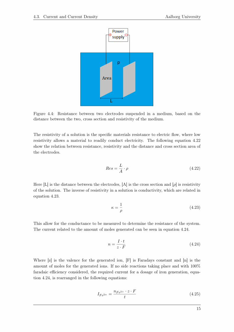
When this is applied to solutions, where the current is moving through an electrolyte, theresistance is determined by the pure solution, whereas for this project is wastewater, whichas mentioned, contain ions and organic matter that would increase or decrease resistance.The resistance in a solution can be estimated by the length and cross section area betweenelectrodes and the resistivity of the solution, shown on figure 4.4.

14

4.3. Current and Current Density Aalborg University

Figure 4.4: Resistance between two electrodes suspended in a medium, based on thedistance between the two, cross section and resistivity of the medium.

The resistivity of a solution is the specific materials resistance to electric flow, where lowresistivity allows a material to readily conduct electricity. The following equation 4.22show the relation between resistance, resistivity and the distance and cross section area ofthe electrodes.

Res =L

A· ρ (4.22)

Here [L] is the distance between the electrodes, [A] is the cross section and [ρ] is resistivityof the solution. The inverse of resistivity in a solution is conductivity, which are related inequation 4.23.

κ =1

ρ(4.23)

This allow for the conductance to be measured to determine the resistance of the system.The current related to the amount of moles generated can be seen in equation 4.24.

n =I · tz · F

(4.24)

Where [z] is the valence for the generated ion, [F] is Faradays constant and [n] is theamount of moles for the generated ions. If no side reactions taking place and with 100%faradaic efficiency considered, the required current for a dosage of iron generation, equa-tion 4.24, is rearranged in the following equations:

IFe2+ =nFe2+ · z · F

t(4.25)

15

Silas. A. C. Duus 4. Theory

dosageFe2+ = Q · c (4.26)

nFe2+

t=dosageFe2+

MFe2+(4.27)

IFe2+ =Q · c · z · FMFe2+

(4.28)

Here [Q] is the flow in[Ls

], [c] the concentration of iron at the outlet in

[ gL

]and [M] is

the molar mass of iron. Equation 4.28 than determines the current needed for a specificeffluent concentration.

4.4 Reactor settings and configurations

For setting up the EC cell the connection and setup of the electrodes can be varied. Theelectrodes can be monopolar and bipolar attuned shown on figure 4.5.

Figure 4.5: Different electrode configuration shown in an electrochemical setup by [6].

The configuration setup showed bipolar electrodes require higher voltage but lower currentto operate, hence the best electrode arrangement is based on yield, cost or efficiency.Bipolar in a series connection showed to be favouring yield, while monopolar is the mostcost effective, due to the lowest energy consumption and high pollutant removal. [6] Sincethe current is related to the amount of ions released seen from equation 4.28, keeping thepotential of the system at a low value to diminsh side reactions from taking place, it isneeded to either reduce the distance between the electrode or have a larger surface area, asseen from equation 4.22. The distance between the electrodes should as short as possible,while still allowing a stream to pass by them. To create an electrode in reasonable size,additional electrodes used will give the surface area of one large electrode, but is easierto replace when the electrodes decompose. Other research have been made using multipleelectrode sets, e.g. 3 anodes and cathode sets. With multiple electrodes used the circuitpath for the electrons are changed and defined by either being serial or parallel connected.For the following equations the subscript [sys] denotes the whole system. For electrodesconnected in a serial connected circuit the current, resistance and potential would follow

16

4.4. Reactor settings and configurations Aalborg University

equations 4.29 to 4.31:

Usys = U1 + U2 + Un... (4.29)

Ressys = Res1 +Res2 +Resn... (4.30)

Isys = I1 = I2 = Constant (4.31)

The potential of the whole system is determined by the each potential drop in the wholesystem, see figure 4.6, while the current of the system remain constant. This is due to theelectrons only having one path to take through the system, and as such will not change.

Figure 4.6: Schematic of a series connected circuit. R in the figure are the same as Res.

For electrodes in a serial connected circuit, the resistance of the system determines thepotential, and as the resistance change due to passivation layer, concentration increaseand distance between the electrodes change as they corrode, a serial connection is notfavourable. If the electrodes however are connected in a parallel circuit, the potential,resistance and current of the system is related in equation 4.32 to 4.34:

Usys = U1 = U2 = Constant (4.32)1

Ressys=

1

Res1+

1

Res2+

1

Resn... (4.33)

Isys = I1 + I2 + In... (4.34)

For this system, the electrons can take several paths across the electrolyte, with the currentof the whole system being a representation of each these paths. Since the resistance still canchange like described before, the potential will remain less affected by this, as the increasein resistance might be around one electrode. However in parallel circuits the potential forthe system will stay the same, even with multiple paths, as such the current would bethe one to drop when the resistance increase at the electrodes. For electrochemistry thepotential determines the reaction taking place, which means the parallel connected circuitgive a larger control of potential side reactions taking place. Therefore this project willchoose parallel connected circuits. A parallel circuit can be seen figure 4.7.

17

Silas. A. C. Duus 4. Theory

Figure 4.7: Schematic of a parallel connected circuit.

For this project the aim is to connect all electrodes in a parallel circuit, to have a constantpotential to avoid generation of unwanted side reactions at high potentials.

4.5 Circuit

When looking at the electrocoagulation cell, a large area is desired, creating a large reactivesurface. However, with increasing quantity of solution and concentrations, the area have toincrease. Often plates are used, which have a directing flow, but with a large plate, the flowmight become laminar at large distances, which would be undesirable for the concentrationof ions, since the diffusion and electron migration would be the primary forces to moveions from the surface to the bulk solution. In this project a cell with rods, placed in aarray with a predefined distance between each rod, would create a more turbulent flow, asseen in picture 4.8.

Figure 4.8: The flow through the cell, seen from the side.

The circles in the figure 4.8 represent the electrodes, each row alternating being cathode

18

4.6. Electrocoagulation process limits Aalborg University

and anode. The distance used for predicting the resistance between the electrodes will bedefined as follows:

Figure 4.9: The shortest distance between an anode and a cathode with the red line.

Figure 4.9 have the shortest distance between an anode and cathode, while the electrodeis enclosed by 4 opposite electrodes. This setup for the flow will disrupt the flow throughthe cell and help with mixing of the bulk.

4.6 Electrocoagulation process limits

When working with EC previous research covered a number of parameters which mayinfluence the overall efficiency of the cell.

4.6.1 Degradation of electrode

During the continued use of the EC cell, the sacrificial anode will be start to corrode, whilethe cathode have shown to create an oxide layer[18], which decrease the efficiency. Thiswill lower the overall release of ions, since less generation of hydroxides will also decreasethe generation of Fe2+, since the reaction is stoichiometric to keep the electron balance.

4.6.2 Alternating and Direct Current

The use of alternating (AC) or direct(DC) current contributes to the overall operation costfor the EC. DC is the most commonly used power supply for EC, but [19] reported thatAC can be superior in operation, where they reported an removal efficiency increase whenusing AC, and the power consumption lowered overall. This can be due to the decrease ofthe passivation layer which might form on the cathode, and was reported by [11, 17].

4.6.3 Mass transport limit

4.7 COMSOL

In this project COMSOL multi-physics 5.5 will be used to create virtual models of ECcells. All simulated designs can be found in the enclosed appendix folder. The aim for theCOMSOL simulations is to evaluate fluid dynamics and in place of physical construction.In COMSOL two physic studies will be used, Laminar and turbulent fluid flows. For thelaminar flow model, this physics is simply selected in the COMSOL multiphysics interface,

19

Silas. A. C. Duus 4. Theory

using a mesh system to solve the continuum mechanics of the generate structure. Whenmeasuring the turbulence fluid dynamics, a selection of models are available:

• Algebraic γPlus model.• L-VEL model.• κ− ε model.• κ− ω model.

The first two models, L-VEL and γPlus, simulate the eddy viscosity using algebraicexpressions using the local fluid velocity against the distance to the closest wall. Transportequations are not solved in these models. These models are the least expensive incomputation power, however also least accurate models.The κ− ε and κ− ω model are similar in solving. Here two variables are calculated, firstthe turbulent kinetic energy, k, and the rate of dissipation of turbulence kinetic energy εor specific rate of dissipation of kinetic energy ω. In these models wall functions will beused, which is computation for fluid dynamics near the wall, see figure 4.10. As simulationapproach the wall, the mesh of the geometry needs to be finer, increasing simulation times.These are the most common used turbulence models used in COMSOL, while also beingthe least computation expensive. For this project the κ − ε is used, as the model is wellsuited for flow around complex geometries, where κ−ω model are used for strong curvatureseen in pipes.[4]

Figure 4.10: Schematic of the layers and wall functions which are used by COMSOL.[2]

20

Experimental setups 5This section will cover the simulation setup for each simulation in COMSOL multiphysicswhere the fluid dynamics will be investigated. Fluid dynamics will simulate the flowthrough an EC, and measure the pressure difference between laminar and turbulentflow. Parametric sweeps models will be applied, to increase the flow through the cell,to investigate the flow patterns around the electrodes.

5.1 COMSOL - Cell building

This section will cover the aspects of building a EC cell in COMSOL multiphysics. Firsta model wizard is used to create a 3D model.

Figure 5.1: The wizard setup from new file in COMSOL multiphysics. Model wizard isselected.

Afterwards a 3D model is selected and physics are selected.

Figure 5.2: Selection of dimension, 3D for this project.

21

Silas. A. C. Duus 5. Experimental setups

Figure 5.3: The figure show a list of physics COMSOL can use, for these simulationsturbulent and laminar flows will be used under Single-Phase Flow. When physics areselected they appear in the lower confirmation box.

Laminar physics is a singular physics model which is selected, however for the turbulentmodel several physics can be chosen, where each model from top to bottom, will increasethe computation time, but increase the precision and accuarcy of the model. For thissimulation the turbulent flow κ−ε is used. When all physics are selected the Study buttonis clicked in figure 5.3 to select a study, which is either time dependant or stationary. For

22

5.1. COMSOL - Cell building Aalborg University

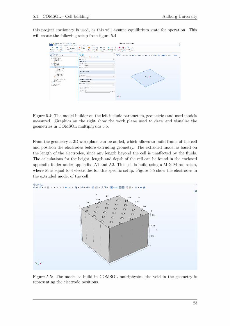
this project stationary is used, as this will assume equilibrium state for operation. Thiswill create the following setup from figure 5.4

Figure 5.4: The model builder on the left include parameters, geometries and used modelsmeasured. Graphics on the right show the work plane used to draw and visualise thegeometries in COMSOL multiphysics 5.5.

From the geometry a 2D workplane can be added, which allows to build frame of the celland position the electrodes before extruding geometry. The extruded model is based onthe length of the electrodes, since any length beyond the cell is unaffected by the fluids.The calculations for the height, length and depth of the cell can be found in the enclosedappendix folder under appendix; A1 and A2. This cell is build using a M X M rod setup,where M is equal to 4 electrodes for this specific setup. Figure 5.5 show the electrodes inthe extruded model of the cell.

Figure 5.5: The model as build in COMSOL multiphysics, the void in the geometry isrepresenting the electrode positions.

23

Silas. A. C. Duus 5. Experimental setups

Figure 5.6 in and out flow for the cell.

Figure 5.6: The blue area on the left figure show inlet and the right figure show the outlet.

A mesh is then generated for the structure, as small control volumes, which are used formeasuring the continuum mechanics affecting the fluid dynamics of the water through thecell. The mesh generated are shown in figure 5.7.

Figure 5.7: Illustrates the coarse mesh modelled on the cell. The tetrahedrons are refinednear the surfaces and boundaries using a mapped generation of finer mesh, due to thedistance between the electrodes and the walls of the cell, where coarse is free tetrahedronsare too large to model sufficiently.

Once a mess is generated under each physics, laminar and turbulent respectively, inlet andoutlet surfaces are selected. Under each study a parametric sweep is added, which will runthe simulation multiple times, and increase the flow through the cell.

24

Results 66.1 Cell design

In this project the cell design was based on having as much surface area available aspossible, while using predefined parameters. The following table show the initial selectedvalues for the cell.

Parameter Value Unit variable rangeFlow 0.05 [ gL ] 0.05 [ gL ] to 3 [ gL ]

Current Density 17.78 [Ampm2 ] 15 [Amp

m2 ] to 20 [Ampm2 ]

Conductivity 0.1 [S/m] -Concentration 0.1 [ gL ] -

Diameter of rods 0.6 [cm] 0.5 [cm] to 0.6 [cm]Electrode sets 16 - 16 anodes and 16 cathodes

Cathode || Anode distance 1.00 [cm] 0.9 [cm] to 1.0 [cm]

Using the parameters, the cell for COMSOL was designed with the rod setup. First thecurrent were determined by equation 4.28, which gave a current for the system to be:

Q · c · z · FMFe2+

= IFe2+ (6.1)

0.05 Lmin · 0.1

gL · 2 · 96485 C

mol

55.85 gmol · 60[s]

= 0.288Amp (6.2)

This allowed to determine the required surface area needed, to generate the current, atthe predefined current density.

J =I

A A =

I

J(6.3)

0.288Amp

17.78Ampm2

= 161.9[cm2] (6.4)

This surface area will be divided by the desired amount of electrodes, for this case 16anodes and cathodes will be used giving a total surface area of a single electrode to be10.12 cm2. The length of each electrode was determined using the surface area, and thedesired diameter. The following equation r is the radius of the cylinder shaped rods, andthe height is the length of the rods.

Asurface = 2 · π · r · h h =Asurface

2 · π · r(6.5)

10.12[cm2]

2 · π · 0.25cm= 5.36[cm] (6.6)

25

Silas. A. C. Duus 6. Results

This was used to generate the structure in COMSOL and the fluid dynamics was calculatedon this. The length of the cell was made to have the electrodes in an array matrix withcathode/anode distance being 0.9 [cm]. They were setup in a 4X4 array.

Figure 6.1: COMSOL worksheet of the build cell, with the electrodes in a 4X4 array setup.

The distance between each electrode was used to decide the length of the cell and width ofthe cell. The height of the cell was set to the length of the electrodes, as anything beyondwould not be simulated, or affect the simulations. The distance between two cathodeswere determined using figure 6.2

Figure 6.2: The fixed distance is set at the surface of the electrodes. The distance c isbased on the space between electrodes to the mass center of the rods. Distance b is themass center distance between two rows of electrodes and distance a is the mass centerdistance between two columns. The angles on distance c are set to 45◦.

The distance between two same polarity electrodes are equal to distance "a" times 2. For

26

6.2. COMSOL simulations Aalborg University

the first and the last electrode in each set, the length of the cell must be increased by theradius of the rods, since the distance "a" include half the distance of the current rod andthe next rod. The length of the cell calculated using:

a = c · cos(45◦) (6.7)

c = 0.9[cm] + 0.6[cm] (6.8)

a = 0.9[cm] + 0.6[cm] · cos(45◦)⇒ a = 1.06[cm] (6.9)

lengthcell = a · 2 · (4− 1) + d (6.10)

lengthcell = 1.06[cm] · 2 · 3 + 0.6[cm]⇒ lengthcell = 7.92[cm] (6.11)

Here the distance between electrodes is 0.9 [cm] and the diameter is 0.6, as the radiusof each rod are used, to get to the center for each. This was the dimensions used forgenerating the cell in COMSOL.

6.2 COMSOL simulations

In COMSOL for the study, everything was measured at stationary, assuming the reactoris at steady state.

6.2.1 laminar

For laminar simulations a single model in COMSOL is used, assuming a everything in therector flows at laminar conditions. The model simulates the change in velocity and thepressure through the cell, which can be seen from figure 6.3 and 6.4.

Figure 6.3: COMSOL simulation of the velocity change through the cell. The flow of thecell can be seen in the top left corner for each Cell defined as Q. The legend show thevelocity measured in m

s and how it increases from blue to red.

27

Silas. A. C. Duus 6. Results

Figure 6.4: COMSOL simulation of the pressure change through the cell. The flow of thecell can be seen in the top left corner for each Cell defined as Q. The legend show thepressure measured in [Pa] and how it increases from blue to red.

For the velocity in laminar conditions, the functions near the wall are not calculated, whichis seen as the no change in velocity on both high and low speed, however, inside the cell,the increase in velocity does happen around rod, this is shown in a slice velocity seen infigure 6.5

Figure 6.5: It can be seen around the rods the velocity increase, due to the disturbance ofthe rods.

From the pressure simulation, it seems the first half of the cell is under higher pressure,and dissipates as the fluid passes the next set of rods.

6.2.2 turbulent

For the turbulent simulations, the κ − ε model is used. Evaluating the data fromCOMSOL are made using convergence plots and wall resolutions, when simulatingturbulent fluid dynamics. In COMSOL the wall resolution should be low as possible,otherwise the computational domains exceed the walls, and movement is calculated through

28

6.2. COMSOL simulations Aalborg University

the boundary layers, such as the electrodes. For this model the wall resolution showedpromising results, seen in picture 6.6.

Figure 6.6: COMSOL simulation of the wall resolution for the highest flow turbulentmodel, with a flow of 3 L

min .

It can be seen from this picture that the wall resolution is 11.06 everywhere, which is thelowest value and best resolution in COMSOL. This is seen at the highest flow rate of 3L

min , which means this meshing is fine enough for fluid simulations. As mention in section5, the meshing generated for this model is Coarse in the bulk and made a finer mappedmesh near the electrodes and walls, to improve the accuracy of the model and decreasethe computation time. Next figures show the velocity of the lowest and highest flow ratethrough the cell, figure 6.7.

Figure 6.7: COMSOL simulation of velocity for the highest and lowest flow rates of 0.5L

min to 3 Lmin .

29

Silas. A. C. Duus 6. Results

Around the rods, the velocity can be seen to change, and increase as the stream meets newrods. On the front of the rods, the velocity seem to increase near the surface of the rod,compared to the back of the rods. The rods around the edges of the cell, experience theleast change in velocity, while for the cell setup, a slight space is made between the rodson the edges and the wall of the cells. The low flow rate have the higher velocity of thenear the rods at the wall of the cell.

Figure 6.8: COMSOL simulation of pressure change for the highest and lowest flow ratesof 0.5 L

min to 3 Lmin .

The pressure in the cell is less affected by the rods, compared to the laminar flow model,and the pressure change decrease through the cell. ¨

30

Discussion 77.1 Discussion

The potential attained by generating the COMSOL model, have a current of 0.288 [Amp],and with the specific conductivity of wastewater from [], the resistance of the circuit canbe determined as 98.90 [Ohm], however as the cell is using 16 electrodes the resistance ofthe system become as equation 4.33.

1

Rsys=

1 · 16

98.9[ohm]⇒ Rsys =

98.9[Ohm]

16(7.1)

Rsys = 6.18[Ohm] (7.2)

This means the effective resistance of the parallel system is far lower, then the resistancefor a single electrode set. The potential can now be estimated using Ohm’s law.

Usys = I ·Res (7.3)

0.288[Amp] · 6.18[Ohm] = 1.78[V ] (7.4)

(7.5)

This would allow the operation of releasing iron into the solution, having the operationpotential at 1.78 [V], and getting a concentration in solution to 0.1 [ gL ]. However, asthe resistance is dependant on the conductivity of the electrolyte, as the concentrationof iron and hydroxides increase near the surface of the electrode, the resistance willincrease. Between the two circuits, series and parallel, the parallel will experience lessoverall resistance increase, as each electrode will be a single circuit, as the current willremain the same. To get the most accurate conductivity of the electrolyte, it is better touse the molar conductivity, seen in equation 7.6.

Λm =κ

C(7.6)

Here the Λm denotes the molar conductivity and κ is the conductivity of the electrolyteand C is the molar concentration of the electrolyte.

7.1.1 COMSOL

In COMSOL the fluid dynamics was only simulated, as the species transport model wasnot giving proper results. To simulate the electrolytic resistance, change in potential,and release of iron and hydroxides in COMSOL some limitations were observed. Thepassivation layer which have been reported in [18], cannot be simulated in COMSOL, asthe simulation will only show the operation at steady state.

31

Silas. A. C. Duus 7. Discussion

The cell was designed to avoid having flow behind the edges of the electrodes near thewall, since the no counter electrode would be near. This was due to ensure most of thefluid flow in passed near an electrode, within the shortest distance of 1 [cm]. But whensimulation, to avoid a meshing difficulties near the electrodes at the wall and the wall, aspace was added to encounter that.

32

Conclusion 8It can be conclude the theoretical creation of a cell based on a fixed current density andconcentration generated a structure in a parallel circuit, showing a potential being lowerthan 1.8 [V]. COMSOL multiphysics as strong tool to simulate the fluid dynamics.

33

Perspectives 9To work further with this project a physical cell would be build of the same dimensions asthe one generated in COMSOL. Here the release of iron ions based on the current and flowrate would be measurable and compared to COMSOL simulation. This would be doneon wastewater, taken from before primary sedimentation, secondary sedimentation anddewatering treatment. The release of iron could be measured using qualitative inorganicanalysis using thiocyanate, to create coordination complexes in a spectrophotometer. Thiscomplex follows Le Chatelier’s principle, and along with ICP can determine Fe2+ and Fe3+

in solution. Treating the wastewater with oxygen to measure the change in Fe2+/Fe3+

compared to untreated wastewater. For COMSOL the simulations of mass transport usingeither Primary, secondary or tertiary current distribution. This can be used to understandthe how the composition of the fluid, concentration overpotential and kinetics affect theoverall process. This can be seen from figure 9.1.

35

Silas. A. C. Duus 9. Perspectives

Figure 9.1: This figure is a guideline for which model to use depending on model variablesand parameters. [4]

36

Bibliography

[1] Hvad sker der med det spildevand, du sender ud i kloakken? URL https://www.vandcenter.dk/viden/spildevand.

[2] Simulating Turbulent Flow in COMSOL Multiphysics®. URL https://www.comsol.com/video/simulating-turbulent-flow-in-comsol-multiphysics.

[3] Sulfur Cycle - an overview | ScienceDirect Topics. URL https://www.sciencedirect.com/topics/earth-and-planetary-sciences/sulfur-cycle.

[4] Which Current Distribution Interface Do I Use? | COMSOL Blog. URL https://www.comsol.com/blogs/current-distribution-interface-use/.

[5] Nafaâ Adhoum, Lotfi Monser, Nizar Bellakhal, and Jamel Eddine Belgaied.Treatment of electroplating wastewater containing Cu2+, Zn 2+ and Cr(VI) byelectrocoagulation. Journal of Hazardous Materials, 112(3):207–213, 8 2004. ISSN03043894. doi: 10.1016/j.jhazmat.2004.04.018.

[6] Zakaria Al-Qodah and Mohammad Al-Shannag. Heavy metal ions removal fromwastewater using electrocoagulation processes: A comprehensive review, 11 2017.ISSN 15205754.

[7] Pablo Cañizares, Carlos Jiménez, Fabiola Martínez, Cristina Sáez, and Manuel A.Rodrigo. Study of the electrocoagulation process using aluminum and iron electrodes.Industrial and Engineering Chemistry Research, 46(19):6189–6195, 9 2007. ISSN08885885. doi: 10.1021/ie070059f.

[8] John C. Crittenden, R. Rhodes Trussell, David W. Hand, Kerry J. Howe, andGeorge Tchobanoglous. MWH’s Water Treatment: Principles and Design: ThirdEdition. John Wiley and Sons, 3rd ed. edition, 3 2012. ISBN 9780470405390. doi:10.1002/9781118131473.

[9] Jing Ding, Liangliang Wei, Huibin Huang, Qingliang Zhao, Weizhu Hou, Felix TettehKabutey, Yixing Yuan, and Dionysios D. Dionysiou. Tertiary treatment of landfillleachate by an integrated Electro-Oxidation/Electro-Coagulation/Electro-Reductionprocess: Performance and mechanism. Journal of Hazardous Materials, 351:90–97, 6 2018. ISSN 03043894. doi: 10.1016/j.jhazmat.2018.02.038. URL https://linkinghub.elsevier.com/retrieve/pii/S0304389418301262.

[10] · Driftsomkostninger and · Levetid. ØKONOMI: MILJØ: · Energiforbrug · CO2 udled-ning CSR: · Arbejdsmiljø · Automatisering · Baeredygtighed FORBEHANDLINGPROCES SL AMBEHANDLING UDEN FOR HEGNET SERVICE. Technical re-port. URL www.stjernholm.dk.

37

Silas. A. C. Duus Bibliography

[11] Murat Eyvaz, Mustafa Kirlaroglu, Tugrul Selami Aktas, and Ebubekir Yuksel.The effects of alternating current electrocoagulation on dye removal from aqueoussolutions. Chemical Engineering Journal, 153(1-3):16–22, 11 2009. ISSN 13858947.doi: 10.1016/j.cej.2009.05.028.

[12] Sergi Garcia-Segura, Maria Maesia S.G. Eiband, Jailson Vieira de Melo, andCarlos Alberto Martínez-Huitle. Electrocoagulation and advanced electrocoagulationprocesses: A general review about the fundamentals, emerging applications and itsassociation with other technologies. Journal of Electroanalytical Chemistry, 801:267–299, 9 2017. ISSN 1572-6657. doi: 10.1016/J.JELECHEM.2017.07.047. URLhttps://www.sciencedirect.com/science/article/pii/S1572665717305337.

[13] Daniel C. Harris. Quantitative Chemical Analysis. In Quantitative Chemical Analysis,chapter Chapter 13, pages 279–307. W.H. Freeman and Co, 8th ed. edition, 2010.ISBN 978-1-4292-1815-3. doi: 10.1142/8727.

[14] Daniel C. Harris. Quantitative chemical analysis. In Quantitative Chemical Analysis,chapter Appendix H, pages AP20–AP27. W.H. Freeman and Co, 8th ed. edition, 2010.ISBN 978-1-4292-1815-3. doi: 10.1142/8727.

[15] Peter K. Holt, Geoffrey W. Barton, and Cynthia A. Mitchell. The future forelectrocoagulation as a localised water treatment technology. Chemosphere, 59(3):355–367, 2005. ISSN 00456535. doi: 10.1016/j.chemosphere.2004.10.023.

[16] Ville Kuokkanen, Toivo Kuokkanen, Jaakko Rämö, and Ulla Lassi. RecentApplications of Electrocoagulation in Treatment of Water and Wastewater—AReview. Green and Sustainable Chemistry, 03(02):89–121, 2013. ISSN 2160-6951.doi: 10.4236/gsc.2013.32013.

[17] Mohammad Y.A. Mollah, Paul Morkovsky, Jewel A.G. Gomes, Mehmet Kesmez,Jose Parga, and David L. Cocke. Fundamentals, present and future perspectivesof electrocoagulation. Journal of Hazardous Materials, 114(1-3):199–210, 10 2004.ISSN 03043894. doi: 10.1016/j.jhazmat.2004.08.009.

[18] Dina T. Moussa, Muftah H. El-Naas, Mustafa Nasser, and Mohammed J. Al-Marri.A comprehensive review of electrocoagulation for water treatment: Potentials andchallenges, 1 2017. ISSN 10958630.

[19] Subramanyan Vasudevan, Jothinathan Lakshmi, and Ganapathy Sozhan. Effects ofalternating and direct current in electrocoagulation process on the removal of cadmiumfrom water. Journal of Hazardous Materials, 192(1):26–34, 8 2011. ISSN 03043894.doi: 10.1016/j.jhazmat.2011.04.081.

[20] Eilen A. Vik, Dale A. Carlson, Arild S. Eikum, and Egil T. Gjessing. Electrocoagula-tion of potable water. Water Research, 18(11):1355–1360, 1984. ISSN 00431354. doi:10.1016/0043-1354(84)90003-4.

38