Design and modelling of optimal driveline control strategy for an electric racing car with rear in-line motors Guo, M. Submitted version deposited in CURVE March 2016 Original citation: Guo, M. (2015). Design and modelling of optimal driveline control strategy for an electric racing car with rear in-line motors. Unpublished PhD Thesis. Coventry: Coventry University Copyright © and Moral Rights are retained by the author. A copy can be downloaded for personal non-commercial research or study, without prior permission or charge. This item cannot be reproduced or quoted extensively from without first obtaining permission in writing from the copyright holder(s). The content must not be changed in any way or sold commercially in any format or medium without the formal permission of the copyright holders. Some materials have been removed from this thesis due to third party copyright. Pages where material has been removed are clearly marked in the electronic version. The unabridged version of the thesis can be viewed at the Lanchester Library, Coventry University.

CURVE is the Institutional Repository for Coventry University http://curve.coventry.ac.uk/open

DESIGN AND MODELLING OF OPTIMAL DRIVELINE

CONTROL STRATEGY FOR AN ELECTRIC RACING CAR

WITH REAR IN-LINE MOTORS

Meng Guo

A thesis submitted in partial fulfilment of the

requirements of the Coventry University

for the degree of Doctor of Philosophy

August 2015

Abstract

Interest in electric vehicles (EVs) has increased rapidly over recent years from both

industrial and academic viewpoints due to increasing concerns about environmental

pollution and global oil usage. In the automotive sector, huge efforts have been

invested in vehicle technology to improve efficiency and reduce carbon emissions

with, for example, electric vehicles. Nowadays, the safety and handling of electric

vehicles present new tasks for vehicle dynamics engineers due to the changes in

weight distribution and vehicle architecture. This thesis focuses on one design area

of the electric vehicle – torque vectoring control – with the aim of investigating the

potential benefits of improved vehicle dynamics and handling for EVs.

A full electric racing car kit developed by Westfield Sportcars based on an in-line

motors design has been modelled in ADAMS with typical subsystems, and then

simulated with computer-based kinematic and dynamic analyses. Thus, the

characteristics of the suspensions and the natural frequencies of the sprung and

unsprung masses were found, so that the model was validated for further simulation

and investigation. Different architectures of the EVs, namely the in-line motors and

the in-wheel motors, are compared using objective measurements. The objective

measurements predicted with kinematics, dynamics and handling analyses confirm

that the architecture of the in-line motors provides a superior dynamics performance

for ride and driveability. An Optimal Driveline Control Strategy (ODCS) based on the

concept of individual wheel control is designed and its performance is compared with

the more common driveline used successfully in the past. The research challenge is

to investigate the optimisation of the driving torque outputs to control the vehicle and

provide the desired vehicle dynamics. The simulation results confirm that active yaw

control is indeed achievable.

The original aspects of this work include defining the characteristics and linearity of

the project vehicle using a novel consideration of yaw rate gain; the design and

development the Optimal Driveline Control Strategy (ODCS); the analysis and

modelling the ODCS in the vehicle and the comparison of the results with

conventional drivelines. The work has demonstrated that valuable performance

benefits result from using optimal torque vectoring control for electric vehicle

I

Contents

Index for Figures ....................................................................................................... IV

Index for tables ........................................................................................................ VIII

Annotations ............................................................................................................... IX

Abbreviations ............................................................................................................. X

Acknowledgement ..................................................................................................... XI

1. Introduction ......................................................................................................... 1

1.1 Pollution and fuel consumption ..................................................................... 1

1.2 Developing electric vehicles .......................................................................... 1

1.3 Aim and objectives ........................................................................................ 3

2 Literature Review ................................................................................................ 6

2.1 Introduction ................................................................................................... 6

2.2 Electric Vehicle .............................................................................................. 6

2.3 Drivetrain Designs ......................................................................................... 7

2.3.1 Conventional mechanical drivetrains ...................................................... 7

2.3.2 Drivetrains for electric vehicle ................................................................. 8

2.4 Vehicle dynamics control ............................................................................ 10

2.4.1 Direct Yaw Control ................................................................................ 11

2.4.2 Torque Vectoring System ..................................................................... 13

2.5 Handling Control for electric vehicles .......................................................... 18

2.5.1 Driver Model ......................................................................................... 22

2.5.2 Importance of control strategy .............................................................. 24

2.6 Concluding remarks .................................................................................... 26

3. Modelling Electric Vehicle in ADAMS ................................................................ 29

3.1 Introduction ................................................................................................. 29

3.2 Project Vehicle ............................................................................................ 29

3.2.1 Driveline ................................................................................................ 30

3.2.2 Chassis and Suspension system .......................................................... 32

II

3.3 Modelling project vehicle ............................................................................. 33

3.3.1 Vehicle Body ......................................................................................... 34

3.3.2 Suspension System .............................................................................. 36

3.3.3 Steering System ................................................................................... 40

3.3.4 Aerodynamic Effects ............................................................................. 42

3.3.5 Driveline Modelling ............................................................................... 44

3.4 Tyre modelling ............................................................................................. 47

3.4.1 Modelling virtual tyre rig ........................................................................ 47

3.4.2 Tyre model for project vehicle ............................................................... 48

3.5 Conclusion .................................................................................................. 51

4 Measurement and analysis of the virtual model ................................................ 53

4.1 Introduction ................................................................................................. 53

4.2 Kinematic analysis ...................................................................................... 53

4.2.1 Quarter vehicle modelling ..................................................................... 54

4.2.2 General approach for kinematic analysis .............................................. 55

4.2.3 Suspension measurements .................................................................. 56

4.3 Dynamic analysis ........................................................................................ 60

4.3.1 Total degrees of freedom ...................................................................... 61

4.3.2 Dynamic model ..................................................................................... 62

4.4 Steady-State Handling analysis .................................................................. 68

4.4.1 Driver behaviour modelling – a ‗path following‘ controller ..................... 68

4.4.2 Driver behaviour modelling – a ‗survey‘ controller ................................ 74

4.4.3 Steering torque input ............................................................................ 75

4.5 Simulation results ........................................................................................ 77

4.5.1 Steady state cornering behaviour ......................................................... 77

4.5.2 Path following behaviour....................................................................... 78

4.5.3 Vehicle linearity .................................................................................... 79

4.6 Conclusion .................................................................................................. 81

5. Comparison of architecture for electric vehicle ................................................. 83

5.1 Introduction ................................................................................................. 83

5.2 Architecture of in-wheel motors vehicle ....................................................... 83

5.3 Modelling and validating of in-wheel motors vehicle ................................... 86

III

5.4 Modelling architecture of in-line motors vehicle........................................... 88

5.5 Simulation Results ...................................................................................... 91

5.3.1 Analysis of ride comfort ........................................................................ 91

5.3.2 Analysis of drivability check ................................................................ 100

5.5 Conclusion ................................................................................................ 107

6 Torque vectoring system with in-line motors ................................................... 109

6.1 Introduction ............................................................................................... 109

6.2 Basic principles ......................................................................................... 110

6.3 Optimal Driveline Control Strategy (ODCS) .............................................. 114

6.3.1 Definitions of Desired Dynamics Behaviour ........................................ 116

6.3.2 Secondary Control .............................................................................. 125

6.3.3 Advanced Torque Vectoring Control (ATVC) ...................................... 129

6.4 Simulation results ...................................................................................... 136

6.4.1 Steady state cornering ........................................................................ 136

6.4.2 Double lane change ............................................................................ 141

6.5 Conclusion ................................................................................................ 147

7. Conclusions and future work ........................................................................... 149

7.1. Summary and conclusions ........................................................................ 149

7.2. Future work ............................................................................................... 153

Bibliography ........................................................................................................... 154

Appendix ................................................................................................................ 161

IV

Index for Figures

Figure 2-1 Acceleration cornering performance ...................................................... 13

Figure 2-2 Schematic of the active limited-slip differentialError! Bookmark not

defined.

Figure 2-3 Vectoring torque acting on rear right and left wheels ............................. 15

Figure 2-4 Effect of torque vectoring ........................................................................ 15

Figure 2-5 Left-Right Torque Vectoring Concept ...................................................... 17

Figure 2-6 Schematics of recent torque vectoring systems ...................................... 17

Figure 2-7 Wide lane change at 70km/h (dry asphalt) .............................................. 21

Figure 2-8 Control strategy for brake-based torque vectoring .................................. 24

Figure 2-9 Control structure for torque vectoring .........Error! Bookmark not defined.

Figure 2-10 Schematic diagram of the driving control algorithm .............................. 26

Figure 3-1 Architecture of Westfield i-Racer ............................................................. 30

Figure 3-2 The position of the electric motors .......................................................... 31

Figure 3-3 The position of the battery package ........................................................ 31

Figure 3-4 The pictures for the chassis and suspensions ........................................ 32

Figure 3-5 The pictures of the front and rear suspensions ....................................... 32

Figure 3-6 Westfield i-Racer model in ADAMS/View ................................................ 33

Figure 3-7 The method for locating vehicle centre of mass height ........................... 35

Figure 3-8 The actual front and rear suspensions .................................................... 36

Figure 3-9 Front and rear suspension model in ADAMS/View ................................. 37

Figure 3-10 The 2D curve for the nonlinear damper ................................................ 38

Figure 3-11 The parts connected by the correct joints ............................................. 40

Figure 3-12 Modelling steering system in ADAMS ................................................... 41

Figure 3-13 The steering ratio for Westfield i-Racer model ...................................... 42

Figure 3-14 Aerodynamic drag forces in the lateral and longitudinal direction ........ 43

Figure 3-15 The motors position of the project vehicle ............................................. 44

Figure 3-16 Modelling the driveline in ADAMS/View ................................................ 45

Figure 3-17 The tyre test rig model .......................................................................... 48

Figure 3-18 Lateral Force Vs Slip Angle tested on the Virtual Tyre Test Rig ........... 51

Figure 3-19 Self Aligning Moment vs Slip Angle ...................................................... 51

Figure 4-1 Modelling the front of the quarter project vehicle .................................... 54

Figure 4-2 Kinematic simulation for suspension system........................................... 56

V

Figure 4-3 Half Track Change Vs Bump Movement (Front) ................................... 179

Figure 4-4 Wheel Recession Vs Bump Movement (Front) .................................... 180

Figure 4-5 Steering Axis Inclination Vs Bump Movement (Front) ........................... 180

Figure 4-6 Ground Level Offset Vs Bump Movement (Front) ................................. 180

Figure 4-7 Castor Angle Vs Bump Movement (Front) ............................................ 181

Figure 4-8 Suspension Trail Vs Bump Movement (Front) ...................................... 181

Figure 4-9 Steer Angle Vs Bump Movement (Front) .............................................. 181

Figure 4-10 Half Track Change Vs Bump Movement (Rear) .................................. 182

Figure 4-11 Wheel Recession Vs Bump Movement (Rear) .................................... 182

Figure 4-12 Steer Axis Inclination Vs Bump Movement (Rear) .............................. 183

Figure 4-13 Ground Level Offset Vs Bump Movement (Rear) ................................ 183

Figure 4-14 Castor Angle Vs Bump Movement (Rear) ........................................... 183

Figure 4-15 Suspension Trail Vs Bump Movement (Rear) ..................................... 184

Figure 4-16 Camber Angle Vs Bump Movement (Rear) ......................................... 184

Figure 4-17 Steer Angle Vs Bump Movement (Rear) ............................................. 184

Figure 4-18 Two degrees of freedom quarter vehicle model .................................... 60

Figure 4-19 The dynamic model for modal solution ................................................. 63

Figure 4-20 Animations of the modes at primary ride behaviour .............................. 66

Figure 4-21 Animations of the modes at wheel hop behaviour ................................. 67

Figure 4-22 Explanation of Ground Plane Velocity ................................................... 70

Figure 4-23 Explanation of Demanded Yaw Rate .................................................... 71

Figure 4-24 Path curvature for steady state cornering ............................................. 72

Figure 4-25 Steering torque acting on steering wheel .............................................. 76

Figure 4-26 Steering input for the ‗path following‘ model.......................................... 76

Figure 4-27 The explanation of Under-steer or Over-steer ....................................... 77

Figure 4-28 Determination of the project model ....................................................... 78

Figure 4-29 The model runs at the steady-state cornering ....................................... 78

Figure 4-30 Demanded Yaw Rate Vs Front Axle No-Slip Yaw Rate ........................ 79

Figure 4-31 The vehicle lateral acceleration versus target lateral acceleration ........ 80

Figure 4-32 Yaw rate gain versus vehicle speeds .................................................... 81

Figure 5-1 Different design of in-wheel motors ......................................................... 84

Figure 5-2 Protean Electric in-wheel motor .............................................................. 85

Figure 5-3 Architecture of in-wheel motors model .................................................... 86

Figure 5-5 Westfield I-racer with in-wheel motors in ADAMS ................................... 87

VI

Figure 5-6 Model definition for in-wheel motors ....................................................... 88

Figure 5-10 the model geometry of in-line motors for kinematic test ........................ 89

Figure 5-11 Dynamic check model for in-line motor ................................................. 89

Figure 5-12 A full vehicle model for drivability check ............................................... 90

Figure 5-13 Subjective results for ride testing .......................................................... 92

Figure 5-14 Eigenvalues for in wheel motors model................................................. 94

Figure 5-15 The animations for vehicle body ........................................................... 96

Figure 5-16 Front wheel hop modes for in-wheel motors ......................................... 97

Figure 5-17 The plotting of Eigenvalues scatter for in-line motors model ................. 97

Figure 5-18 Road profile for speed bump ............................................................... 100

Figure 5-19 Measured results for wheel hub acceleration ...................................... 100

Figure 5-20 Subjective results of steering behaviour ............................................. 101

Figure 5-21 Ground plane velocity during steady state cornering .......................... 102

Figure 5-22 The trajectories at cornering ............................................................... 103

Figure 5-23 Testing results for centripetal acceleration of in-line and in-wheel motors

............................................................................................................................... 104

Figure 5-24 Double Lane Change Test Course ...................................................... 105

Figure 5-25 Comparison of yaw rate for in-line and in-wheel motors in DLC ......... 106

Figure 5-26 Comparison body slip angle for in-line and in-wheel motors in DLC ... 106

Figure 5-27 Comparison of steering angle for in-line and in-wheel motors in DLC 107

Figure 6-1 Definition of torque vectoring differential ............................................... 110

Figure 6-2 Schematic of a mechanism torque-vectoring differential ....................... 111

Figure 6-3 Explanations of the left-and-right torque vectoring ................................ 112

Figure 6-4 Schematic of Driveline Control Strategy (DCS) ..................................... 115

Figure 6-5 Path curvature spline in ADAMS for cornering ...................................... 119

Figure 6-6 Double lane change test course .................Error! Bookmark not defined.

Figure 6-7 Cosine ramp lane change path visualisation ......................................... 120

Figure 6-8 Optimized lane change path with the behaviours of real driver ............. 120

Figure 6-9 Comparison of the lateral acceleration for cosine and optimised lane

change path ........................................................................................................... 121

Figure 6-10 Path curvature of lane change ............................................................ 121

Figure 6-11 Comparison of desired and actual lateral acceleration ....................... 122

Figure 6-12 Yaw Rate Gain (YRG) for three different vehicles ............................... 123

Figure 6-13 Explanation of torque vectoring authority envelope ............................ 124

VII

Figure 6-14 Motor efficiency map ........................................................................... 135

Figure 6-15 Vehicle model at steady state cornering ............................................. 137

Figure 6-16 Speed compensation with driving torque ............................................ 137

Figure 6-17 Trajectory of vehicle at coasting, with driving torque and TV .............. 138

Figure 6-18 Longitudinal driving forces for rear driving wheels .............................. 139

Figure 6-19 Comparison of Yaw rate correction ..................................................... 140

Figure 6-20 Explanation of torque vectoring control at 40km/h .............................. 142

Figure 6-21 Comparisons of Yaw rate without the speed controller ....................... 142

Figure 6-22 Yaw rate with speed controlled ........................................................... 143

Figure 6-23 Body slip angle for the different driving mode ..................................... 144

Figure 6-24 Explanation of torque vectoring control at 60km/h .............................. 144

Figure 6-25 Variations of yaw rate with the speed controlled at 60 km/h ............... 145

Figure 6-26 Yaw rate variations at 60 km/h ........................................................... 145

Figure 6-27 Variations of body slip angle at 60 km/h ............................................. 146

Figure 6-28 Yaw rate variation at 100km/h ............................................................. 146

Figure 6-29 Yaw rate variation with the speed controlled at 100km/h .................... 147

Figure 6-30 Comparison of body slip angles at 100km/h ....................................... 147

VIII

Index for tables

Table 3-1 Front suspension hard points ................................................................. 178

Table 3-2 Rear suspension hard points .................................................................. 178

Table 3-3 A set data for tyre model .......................................................................... 50

Table 4-1 Total degrees of freedom for the model ................................................... 62

Table 4-2 Display of the eigenvalues in tabular form ............................................... 64

Table 4-3 Explanation of the natural frequencies at each mode .............................. 65

Table 5-1 Display the eigenvalues in tabular form ................................................... 93

Table 5-2 Explanation of natural frequencies at each mode .................................... 93

Table 5-3 Natural Frequencies for in-line motors model ........................................... 98

Table 5-4 Comparison of natural frequencies for in-line and in-wheel motors model99

Table 6-1 The schematic of control modes ............................................................ 129

IX

Annotations

Ax Longitudinal acceleration

Ay Lateral acceleration

b Longitudinal distance of body mass centre from front axle

c Longitudinal distance of body mass centre from rear axle

f Natural frequency

k Path curvature

Ks Spring stiffness

kw Stiffness of equivalent spring at the wheel centre

m Mass of a body

vx Longitudinal velocity

vy Lateral velocity

Fx Longitudinal tractive or braking tyre force

Fy Lateral tyre force

Fz Vertical tyre force

FD Drag force

Af Front axle slip angle

ar Rear axle slip angle

β Side slip angle

δ Steer or toe angle

ω Yaw rate

Demanded yaw rate

Yaw rate error

Front axle no-slip yaw rate

∆T Difference in driving torque

X

Abbreviations

ALSD Active Limited-Slip Differential

AYC Active Yaw Control

ATVC Advanced Torque Vectoring Control

AWD All Wheel Drive

ADAMS Automated Dynamic Analysis of Mechanical Systems

DOF Degrees of Freedom

EV Electric Vehicles

GRG Generalized Reduced Gradient

IC Internal Combustion

LSD Limited-Slip Differential

LQG Linear Quadratic Gaussian

ODCS Optimal Driveline Control Strategy

RWD Rear-Wheel-Drive

SC Speed Compensation

YRE Yaw Rate Error

Yaw Rate Gain YRG

XI

Acknowledgement

I would like to express my gratitude to all those who gave me the possibility to

complete this thesis. I want to thank Coventry University for giving me permission to

commence this thesis in the first instance. I have furthermore to thank my second

supervisor, Dr Gary Wood, who encouraged me to go ahead with my thesis. Also I

would like to thank Mr Damian Harty for his assistance over the period of the

research study.

I am deeply indebted to my director of study Professor Mike Blundell, who gave me

huge support and helped me throughout the research project and in writing up of the

thesis.

Especially, I would like to give my special thanks to my family whose love enabled

me to complete this work.

1

1. Introduction

1.1 Pollution and fuel consumption

Fossil oil is the most important natural resource to support the world economy.

Although recent estimates vary, there is absolutely no doubt that global concerns

about the finite nature of our oil-based energy reserves are well founded (Hirsch,

Bezdek et al. 2005). Global energy demand from all sources is expected to increase

by 1.3 percent per year on average from 2005 to 2030 (ExxonMobil 2007).

Apart from the shortage of oil supply, the concerns in growth of emissions and

pollutions have been discussed every day. In fact, the transportation sector accounts

for about 21 percent of current global fossil fuel CO2 emissions to the atmosphere-

second only to emissions from power production (IPIECA 2004). According to the

Technology Strategy Board (TSB), in the UK it is estimated that transport accounts

for 24% of the UK‘s carbon emissions. Road transport accounts for 80% of this figure

(IME 2009). However, the big challenge to the automotive industry is to be

responsive to both legislation-reducing emissions and the market-growing consumer

demands.

1.2 Developing electric vehicles

There has been a massive resurgence of interest in electric vehicles (EVs) over the

past decade. Many observers now see them as the long-term solution to reducing

vehicle emissions and CO2 usage in comparison to alternative approaches such as

hybrid vehicles, fuel cells or biofuels. The public perception of electric vehicles has

changed dramatically – and recently announced vehicles such as the Tesla roadster

and Chevrolet Volt have reinforced the idea that they are now becoming seriously

competitive products. Not long ago, electric vehicles were still seen as niche

products – and associated more with ‗milk float‘ technology rather than a viable

passenger transport alternative (Chan and Chau, 2001; Husain 2003; Larminie and

Lowry 2003).

2

Massive advances have occurred in battery technology – although the progress has

been gradual and sustained, so that it has not commonly been perceived as a major

breakthrough. The vehicle range available with modern battery sets – such as

Lithium Ion – is now typically of the order of 200km, which makes electric vehicles

widely acceptable for much urban use. The high cost of the batteries is still a

problem and despite a relentless downward price trend, the battery sets are often

supplied on a leasing arrangement rather than a straightforward purchase.

As the electric vehicle market continues to grow, the chassis engineers will place

increasing emphasis on searching for dynamics control due to the new architecture

used on the electric vehicle. This process of continual improvement is central to

vehicle development of safety and handling, and has occurred for example, over

recent decades with vehicle dynamics. The industry has achieved ride comfort and

safety figures that were considered impossible twenty years ago. Of all the green

solutions, battery electric cars have the best dynamics control, individual wheel

control, of both conventional cars and hydrogen fuel-cell cars. Also the driving

efficiency is high, for example, with 1 of electricity, an EV can drive 5525 km;

while using the same amount of electricity to generate hydrogen and to drive a fuel

cell car, the distance is reduced to 1790 km (Randall, 2009).

The electric vehicle as a main test platform for this research focuses on one area of

interest in which dynamics control gains may be achievable for electric powertrains

with individual control motors. As is known, it is commonly argued that one of the

distinct advantages of an electric motor as a motive unit is its torque characteristic; it

can deliver maximum torque from zero speed and throughout the low speed range –

typically up to around 2000 rev/min. Then, the available maximum torque reduces

with speed along the motor‘s maximum power curve. This is a much better

characteristic than that associated with internal combustion engines, which cannot

deliver useful torque at low speeds and because of their relatively narrow torque and

power bands, must be used with multispeed transmissions in order to deliver tractive

power to the vehicle in a suitable form. Typical electric motors have another

desirable feature – their maximum intermittent power is considerably higher than

their rated continuous power. The limiting factor is usually related to controlling the

3

amount of heat build-up. Consequently, good acceleration times can be achieved

providing they are only used for relatively short periods – a situation which

fortunately is typical of normal driving.

1.3 Aim and objectives

The proposed research is focused on active yaw control for electric racing vehicles.

Due to this research being based on an industrial project from Westfield Sportcars,

the company is starting to investigate and develop a full electric racing vehicle that is

called – the Westfield i-Racer. The Westfield engineers have developed the world‘s

first electric race car kit that can be built at home, while also supporting the

requirement of sport racing with zero emissions vehicles.

Initially, the project vehicle with typical sub-systems such as suspension, steering

and driveline system were modelled and assembled so that the requirements of the

vehicle dynamics simulation could be fulfilled. A model audit was needed to ensure a

rigorous system was used in the following research. The audit involved calculating

the mass and inertia properties for the vehicle body and all the components in the

sub-systems, as well as finding the central of mass position for the vehicle body and

the characteristics of the spring and damper in the following section. The tyre-

sourced data is based on the Pacejka 89 version, with the manufacturer‘s

coefficients and the tyre model being run on a computing-based tyre test rig to

indicate all characteristics of the tyre.

When building the project vehicle in computer-based software, the accuracy of the

simulation results relies on the accuracy of the model and the vehicle parameters

used to build the model. Hence, there are several methods available to validate the

vehicle model, such as kinematic and dynamic manoeuvres. In order to verify the

performance of the suspension system, a range of characteristics were determined

through simulation of a quarter vehicle model. The full vehicle model was analysed in

a number of ways that provided information to support the following investigations.

Also, the steady-state cornering manoeuvre was used to define the basic driving

characteristics of the project model.

4

A main difference in architecture for the conventional vehicles is the position of the

Internal Combustion (IC) engine, which can be located at the front, the middle or the

rear of the vehicle; thus influencing the mechanical, such as the Rear-Wheel-Drive

(RWD) or the All-Wheel-Drive (AWD). A novel architecture for the electric vehicle

driveline was designed that has the freedom to move the motors to a single location

in the vehicle, for example, by mounting the motors within individual wheels. In

addition, the electric motors can also be located in the middle of the chassis at the

front, rear or both axles. The recent conformity in electric vehicle architecture, with

high driving eff/iciency of in-wheel motors now on the market, has led to some

complacency in viewing any other architecture. Westfield Sportcars, a producer of

the in-line motors, has commissioned a series of wide-ranging studies into the

effects of vehicle performance. However, a comparison will be introduced that

includes a ride comfort check and drivability check studies using the ADAMS model.

These studies provide a comprehensive overview of the implications of in-wheel and

in-line motors in this particular racing model.

Finally, the most important part of this investigation is to develop and design a novel

Torque Vectoring control strategy. In the literature, active intelligent control systems

for achieving vehicle stability and handling have been developed and implemented to

enhance the safety and performance of the driven vehicle. Some enhancements,

such as the Active Steering System and the Electronic Stability Program, can help

the driver to retain control of their vehicles when the grip between road surface and

tyre is lost. In previous investigations, ABS based Stability Control Systems have

been the principal implementation to accomplish the safety requirements with

adverse road conditions. However, the vehicle speed is degraded while the Stability

Control System implements braking force on four wheels individually to improve the

correct position of the vehicle body. Moreover, the Torque Vectoring (TV) system

can be designed to improve the vehicle handling qualities and avoid the vehicle

speed decrease, or in other words the ‗fun-to-drive‘ aspect. Thus, torque vectoring

can be used to influence the driver experience.

A new control strategy, that is called Optimal Driveline Control Strategy (ODCS), will

be design and/ developed. The ODCS involves three levels of control: Desired

5

Dynamics Behaviours, Secondary Control and Advanced Torque Vectoring Control,

more details of which will be represented in the following section. Reviewing the

basic principles for TV control on the conventional driveline helps to understand how

those control strategies on the pure electric vehicle can be implemented. The

configuration of the ODCS algorithm is clearly shown and each level of control is

explained in detail.

The project vehicle model will be taken into the typical vehicle dynamic simulations,

by running the vehicle model through the steady state cornering and lane change

manoeuvres. The results will be analysed and compared against the project model

running with the different driving modes, assuming the model has the conventional

drivelines, namely Open and Limited Slip Differentials on the rear axle, so that these

will be simulated for the same manoeuvres.

6

2 Literature Review

2.1 Introduction

The previous work on Vehicle Dynamics Control, Direct Yaw Control, Torque

Vectoring and the vehicle dynamics control strategies of Electric Vehicles (EVs) are

reviewed here. The definitions and classifications for a Final Drive Unit are

summarised and the main tools for vehicle dynamics analysis are introduced. For

control strategies, the current situation and the future trends are analysed. Torque

vectoring for electric vehicles has received a substantial amount of attention and

several different designs have been proposed over the past decade. The important

dynamics control strategies for electric racing vehicles, a crucial feature in optimizing

performance and overall performance, are reviewed.

2.2 Electric Vehicle

Vehicle industries and governments around the world appear to have a high level of

interest in electric vehicles, an interest which is growing at a substantial rate. In the

past, commercial vehicles powered by the Internal Combustion engine became

available at the end of the 19th century; while at the same time, an electric vehicle

broke the world land speed record in 1899, becoming the first car to exceed one mile

per minute. At that time, there were three propulsion systems: the electric motor, the

IC engine and the steam engine. Comparing the size and complexities of these

devices, the electric motor was a clear winner; however, it used original lead acid

batteries for the energy storage, which have 300 times lower capacity than that of

the specific energy of the gasoline-driven vehicle.

Based on the global requirement to reduce emissions, both political and

technological sectors have currently been experiencing a resurgence of interest in

electric vehicles supported by emerging battery technologies. Investigations are

mainly focused on energy density, improved specific energy and rechargability

properties. The electric motor has a great advantage in torque characteristic, which

7

means the motor can provide a more desirable spread of torque over the vehicle

speed range compared to that of the IC engine, and also electric vehicle architecture

provides the shortest driveline in contrast to conventional vehicles.

Currently, the most popular design approach for electric vehicle is to connect the

motor to the driven wheels directly, with some designs requiring a transmission unit

between the motor and the wheels. In general, the characteristics of the current

electric motor have two regions – intermittent peak torques and operating torques

that are comparatively lower; the high torques can provide desired acceleration from

very low speeds, and the top speed is constrained by the continuous torques.

Normally, the transmission unit with a fixed gear is used to control the top speed. In

addition, there is another area of interest in the case of an electric vehicle, which is

to investigate how to control the efficiency of the electric motor, so that particular

capacities of the motor are required, namely low speed with high torque, direct-drive

and excellent torque-power densities.

In a similar fashion, plug-in electric vehicle have also become a very topical subject.

For example, the ‗i MiEV‘ from Mitsubishi Motors has been commercially produced

and 200 of these vehicles have been put into the UK for test driving. Using the on-

board charger, the vehicle can be charged with a 100 V or 200 V power source in the

home. The range over one of the driving cycles, for one charge is 160 km, which is

enough for most commuting applications. For example, in the United States, half of

U.S. households have a daily mileage of less than 30 miles per day; 78% of daily

work commuters travel 40 miles or less (Babik 2006).

2.3 Drivetrain Designs

2.3.1 Conventional mechanical drivetrains

An ―Open‖ differential drives the wheels to rotate at different speeds while balancing

the torques between them. A limited slip differential allows for unequal torque

distribution between the wheels, but with a fixed kinematic relationship, and the

torque can only be transferred from the wheel spinning faster to the wheel spinning

8

slower. A torque vectoring system, while retaining the ability to function as a simple

differential, incorporates a means to vary the kinematic ratio across the differential,

thus affecting the torque distribution between the wheels. Torque vector is defined as

the torque difference between the two output torques.

During cornering, the vehicle wheels rotate at different speeds. The differential is

equipped to rotate both the driven wheels with identical torque but different angular

velocity. For this device, the capability to transfer torque and rotation is through three

shafts, one input two outputs. This is found in most vehicles, which allows each of

the driven wheels to rotate at different speeds, while supplying equal torque to each

of them. When cornering, the inside wheel is rolling in a smaller circle than the

outside wheel and without the differential, the inside wheel is spinning and the

outside wheel is dragging. This scenario may cause problematic and unexpected

handling, more tyre wear, and damage to (or possible failure of) the entire drivetrain.

2.3.2 Drivetrains for electric vehicle

Novel concepts of electric vehicle layouts are gaining more and more importance.

The first generation of fully electric vehicles was based on the conversion of internal

combustion engine driven vehicles into electric vehicles, by replacing the drivetrains,

while keeping the same driveline structure; that is, one electric motor drive, which is

located centrally between the driven wheels, and a single-speed mechanical

transmission including a differential. Such a design solution is going to be gradually

substituted by novel vehicle architecture, based on the adoption of individually

controlled electric powertrains, with the unique possibility to improve the vehicle

dynamics control because of their intrinsic high and independent controllability. The

active control of electric powertrains allows the regulation of the distribution of the

driving torques in order to achieve desired steady-state and transient vehicle

dynamics characteristics. At the same time, if implemented through in-wheel motors,

these architectural solutions allow an improvement of the overall vehicle packaging

as less space is required by the powertrain.

Current electric vehicle research is investigating different powertrain configurations,

constituted by one, two, three or four electric motors with different performance in

9

terms of vehicle dynamics behaviour and energy saving targets (Novellis, Sorniotti,

Gruber,2012 and Rinderknecht, Meier,2010) . The possible architectures are shown

in Figure 2-1 (Ehsani, Gao et al.2004), from which it can be seen that mainly two

types of transmissions are used on electric vehicles: multi-gear transmission and

single-gear transmission. Currently, single gear transmissions are used on most EVs.

For example, on the Gulliver U500 design from Tecnobus, the transmission is a

single gear with a fixed ratio of 1:4.37. For configurations like Figure 2-1 (a) and (b),

an electric propulsion motor replaces the IC engine of a conventional vehicle drive

train. The multi-gear transmissions here were originally designed for an engine, not

especially for electric motors. It is perhaps surprising, but there is very little published

research on the potential benefits from connecting the motor to driven wheels

directly by using driving shafts, it can save major components in the transmission

system reduce the weight of entire vehicle and improve driving efficiency.

Figure 2-1 Possible EV configurations (Ehsani, Gao et al. 2004)

This item has been removed due to third party copyright. The unabridged version of the thesis can be viewed at the Lanchester Library, Coventry University.

10

2.4 Vehicle dynamics control

In recent years, several researchers have invested time in, and effort on, the

improvement of vehicle dynamics control, generally focusing on agility, stability,

reliability and linearity to improve handling. These requirements have been applied to

new designs of electric and hybrid vehicles. A Limited-Slip Differential (LSD) is

based on the open differential with a type of gear arrangement that allows the

wheels to have differences in angular velocity and the driving torque. In order to

provide increased stability, alternative control systems are then considered without

the disturbance of brake-based stability control programmes. A Limited-Slip

Differential uses the electronic controller to transfer torque between the driven

wheels. Controlled torque transfer between the driven wheels can generate a yaw

moment that is able to improve the stability of vehicle; and due to the wheel torque

being redistributed without any speed reduction, this improvement in stability is less

intrusive than a brake-based stability control programme.

In general, active steering systems can help the driver to face a critical driving

situation. Zhang (2008) presented a paper that described a multi-body vehicle

dynamic model with an active steering system using a fuzzy logic control strategy.

The multi-body vehicle dynamic model was built in ADAMS and the dynamic

performance of the vehicle could be accurately predicted. The methodology of

control included active front steering and rear wheel steering by wire, to which active

steering at the front axle involved a modified steering angle added to the driver input,

and the rear wheel steering was controlled by wire. This combination was effectively

used to control both body-slip angle and the yaw rate. The controllers used in the

active front and rear steering control were based on a set of fuzzy logic rules to

adjust the body-slip angle and the yaw rate. Optimization of the fuzzy logic control in

both the active front and rear steering system was also represented. Thus, the

simulation results indicated that active front and rear steering using a fuzzy control

logic strategy enabled improved handling and stability of the vehicle comparing the

four-wheel steering with front wheel steering only.

Modification of the vehicle dynamics can also be achieved by controlling the

distribution of lateral forces using the combinations of front and/or rear steering

11

angles in four-wheel steer by wire (Ackermann and Sienel, 1993, Ackermann et al.,

1995, Kohen and Ecrick, 2004 and Vilaplana et al., 2005). Moreover, the

improvement of the vehicle safety capability for emergency avoidance, using the

optimization of both the direct yaw control and active steering control is another

research area of interest (Mokhiamar and Abe, 2002).

According to these previous works, the control designs are only for the development

of the yaw stability control algorithm. The control is based on a model with the

desired vehicle response. The model is a basic vehicle model that can be used to

calculate the desired yaw rate based on the steering input, vehicle speed and road

surface. Moreover, the Limited-Slip Differential designs generate a required torque to

transfer across the axle depending on the error between the desired and actual yaw

rate of the vehicle. The error is fed through a feedback controller, but the Limited-Slip

Differential only develops the yaw moment in the under-steer condition. Also Four-

Wheel Steer and Active steering systems have same limitation.

2.4.1 Direct Yaw Control

Due to unusual external conditions there can be unexpected dangerous behaviours

in vehicle yaw dynamics, such as unexpected side-wind force, different road surface

texture on left-right wheels, and emergency avoidance. Moreover, under-steer may

degrade the handling performance in cornering manoeuvres and cause discomfort to

the human driver. There are, however, a few solutions available in recent years to

solve these issues, and the task is still to carry out intensive research activities in

both practical and analytical studies (see e.g. Börner and Isermann, 2006, Colombo,

2005, Gaspar et al., 2005). In this case the purpose of the study was to modify the

vehicle dynamics and exploit the best combinations in longitudinal and lateral tyre

forces. Also, using the uneven longitudinal driving force on the left and right sides

can control the yaw rate. This approach involved different technologies, for example,

Anti-Lock Braking System (ABS) and Electronic Stability Program (ESP) (Zanten,

2000 and Zanten, 1995) or torque vectoring control using active differentials

(Assadian and Hancock, 2005, Colombo, 2005 and Gerhard, 2005).

12

Assadian, Hancock and Best (2010), describe some developments on mechanical

limited slip differentials which provide a low cost traction solution. However, their

passive nature means that mechanical limited slip differentials cannot adapt to

different conditions and their yaw moment generation potential cannot be used for

vehicle handling or stability control. Active limited slip differentials are becoming

popular as they are able to exploit this potential and also achieve a better traction

compromise due to their ability to adapt to different scenarios. The development of a

control algorithm for an Active Limited-Slip Differential (ALSD) fitted to a RWD sports

saloon vehicle. The ALSD uses a wet friction clutch unit to transfer the torque across

the driven axle, and a driven actuation system with an electric motor controls the

clamping force on the clutch unit through a ball and ramp device.

However, the Limited-Slip Differentials use the wet clutch unit to provide a controlled

left-and-right torque distribution on the front or rear axle, and four-wheel torque

distribution, thus resulting in improved traction control and yaw stability control

performance without being intrusive for the driver. The case speed is equal to

and the clutch always transfers the torque from its faster to its

slower shaft. The direction of torque transfer is determined by the difference in the

wheel speed across the axle. It is restricted to over-steer compensation only when

being used as a yaw stability control device, since only an under-steer torque can be

generated.

Active Yaw Control (AYC) and Super-Active Yaw Control developed by Mitsubishi

Motors (Ushiroda,2003) based on an active differential to modify the torques at the

driven wheels are reviewed in this section. These products were designed and

implemented in the series of the Mitsubishi Lancer Evolution cars, which used a

planetary gear-set, also being used in several Mitsubishi concept models, to support

a greater torque distribution than that of the existing systems.

The simulation results, as shown in Figure 2-2, show that the maximum cornering

performance is obtained by using an AYC model without limitations on torque

transfer. This concept is based on a left-and-right torque vectoring system and the

driving torque is optimally controlled depending on the vehicle conditions. A

comparison of the vehicle with and without the AYC is presented in this paper; and

13

each of the curves shows the maximum lateral acceleration during the cornering

manoeuvre for a given acceleration in the longitudinal direction. It is clear to see that

the acceleration region of the optimally controlled AYC vehicle is 25% larger than

that of the vehicle with only AYC. The torque transfer for the optimally controlled

AYC is 1.8 times larger than the torque transfer amount with AYC alone. Thus, the

increment in the amount of the torque transfer offers a target for which the authors in

this research have identified potential methods to achieve.

Figure 0-2 Acceleration cornering performance (USHIRODA 2003)

Three different torque vectoring strategies which summarise the strategies explained

in above the research have been implemented: i) constant torque distribution

(referred to as the baseline vehicle); ii) torque proportional to the wheel vertical load;

iii) torque distribution which allows achieving the same longitudinal slip ratio at each

wheel.

2.4.2 Torque Vectoring System

Torque vectoring control can have a major impact on the general driving experience.

Most of the time the driver operates the vehicle in steady-state, or slowly varying

conditions, at lateral acceleration levels as below 0.5 g (Pacejka, 2006). During

these sub-limit conditions, the continuous yaw moment control can significantly

improve the vehicle cornering response. As recently pointed out in (Crolla, 2012),

This item has been removed due to third party copyright. The unabridged version of the thesis can be viewed at the Lanchester

Library, Coventry University.

14

―despite the significant volume of theoretical studies of torque-vectoring on vehicle

handling control, there is no widely accepted design methodology of how to exploit it

to improve vehicle handling and stability significantly.‖ To address this issue, novel

tools for the design of torque vectoring control systems have to be proposed and

assessed.

Vehicle steady-state cornering response is usually assessed in terms of its

understeer characteristic, where the dynamic steering wheel angle is the difference

between the actual steering wheel angle and the kinematic steering wheel angle

(Gillespie, 1992). In general, in a passenger car, the dynamic steering wheel angle

increases monotonically and nearly linearly up to a value of lateral acceleration of

about 0.5 g for high friction conditions. Correspondingly, the understeer gradient of

the vehicle is nearly constant. Beyond this linear region is non-linear and tends to an

asymptotic value corresponding to maximum lateral acceleration when the tire friction

limits are reached. In contrast to vehicles without torque vectoring control, where the

specific understeer characteristics are determined by the tyre properties, geometrical

and inertial parameters and the suspension elasto-kinematics (Reimpell, 2001 and

Milliken, 2002), the understeer characteristics of a vehicle equipped with a TV

system can be designed to achieve almost any desired response. For example, the

understeer gradient in the linear part of the characteristic could be imposed. Also,

the width of the linear region could be increased, or the maximum lateral

acceleration could be altered, with the constraints dictated by tyre friction limits

(Zorzutti, 2007).

In addition to the advantages during pure cornering manoeuvres, continuous TV

control has the potential to improve the handling response of a vehicle while braking

or accelerating. Despite the significant influence of accelerating and braking, the

understeer characteristics for non-zero longitudinal acceleration are normally not

considered and analysed. This restriction mainly results from limitations imposed by

the typical vehicle dynamics simulation techniques or testing procedures used to

derive the zero longitudinal acceleration cornering response plots, namely, skid-pad

tests or ramp-steer manoeuvres.

15

Yaw control is effective in order to realise the active safety philosophy that makes

the likely occurrence of an accident small; and the yaw control technology by using

brake based systems has been developed in a large number of products. As a next

step, direct yaw control can be achieved using the right-and-left torque vectoring

control. This system can directly control the yaw moment acting on a vehicle by

vectoring the torques between wheels on either side with minimum energy loss.

Therefore, the strong point of this system is to be able to improve the stability of the

vehicle from the normal condition to the high marginal condition seamlessly

(Ikushima,1995).

Figure 0-1 Vectoring torque acting on rear right and left wheels (Sawase and Ushiroda, 2007)

A concept is shown in Figure 2-3; the torque flow between the right and left wheels

can be controlled by a device, so that it can make on one side of the driving forces

small, and the other side driving forces large. The difference in the longitudinal

driving torque generated on the right-and-left wheels can control the yaw moment

that acts on the vehicle, even if the engine torque and/or braking force are applied.

//Figure 0-2 Effect of torque vectoring (Sawase and Ushiroda, 2007)

This item has been removed due to third party copyright. The unabridged version of the thesis can be viewed at the Lanchester Library, Coventry University.

This item has been removed due to third party copyright. The unabridged version of the thesis can be viewed at the Lanchester Library, Coventry University.

16

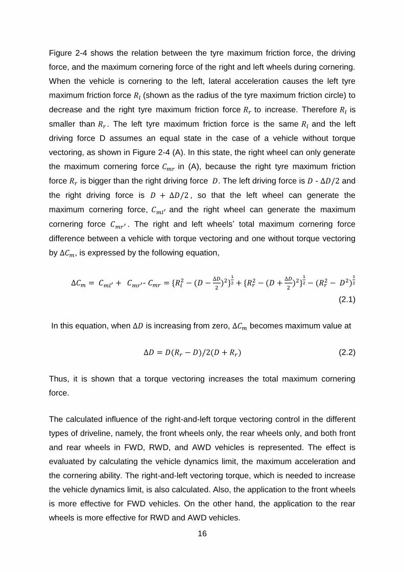
Figure 2-4 shows the relation between the tyre maximum friction force, the driving

force, and the maximum cornering force of the right and left wheels during cornering.

When the vehicle is cornering to the left, lateral acceleration causes the left tyre

maximum friction force (shown as the radius of the tyre maximum friction circle) to

decrease and the right tyre maximum friction force to increase. Therefore is

smaller than . The left tyre maximum friction force is the same and the left

driving force D assumes an equal state in the case of a vehicle without torque

vectoring, as shown in Figure 2-4 (A). In this state, the right wheel can only generate

the maximum cornering force in (A), because the right tyre maximum friction

force is bigger than the right driving force . The left driving force is - and

the right driving force is , so that the left wheel can generate the

maximum cornering force, and the right wheel can generate the maximum

cornering force . The right and left wheels‘ total maximum cornering force

difference between a vehicle with torque vectoring and one without torque vectoring

by , is expressed by the following equation,

-

(2.1)

In this equation, when is increasing from zero, becomes maximum value at

(2.2)

Thus, it is shown that a torque vectoring increases the total maximum cornering

force.

The calculated influence of the right-and-left torque vectoring control in the different

types of driveline, namely, the front wheels only, the rear wheels only, and both front

and rear wheels in FWD, RWD, and AWD vehicles is represented. The effect is

evaluated by calculating the vehicle dynamics limit, the maximum acceleration and

the cornering ability. The right-and-left vectoring torque, which is needed to increase

the vehicle dynamics limit, is also calculated. Also, the application to the front wheels

is more effective for FWD vehicles. On the other hand, the application to the rear

wheels is more effective for RWD and AWD vehicles.

17

Figure 0-3 Left-Right Torque Vectoring Concept

Figure 2-5 shows the concept of left-and-right torque vectoring control in which this

approach has the braking force applied to the left wheel and the same magnitude of

the driving force applied on the right wheel. Thus, it is able to control the yaw rate

directly as required at any time, and the control is without any constraints from the

level of the engine torque, and any conflicts between the torque vectoring control

and the operation of the driver.

Figure 0-4 Schematics of recent torque vectoring systems (Wheals, 2004)

Figure 2-6 shows a comparison between the Ricardo Torque Vectoring systems and

alternatives such as the Mitsubishi EVO VIII device and the Mimura device:

All designs provide permanent drive to the wheels via a differential when the

actuation system is inactive.

This item has been removed due to third party copyright. The unabridged version of the thesis can be viewed at the Lanchester Library, Coventry University.

18

The Ricardo design uses two brakes whereas the Mitsubishi and Mimura

designs both use two clutches. It describes a single brake design.

The Mitsubishi and Mimura designs both use joined planet gears within the

geared stage that force a speed difference between the outputs.

The Ricardo Torque Vectoring™ device uses joined sun gear, which requires

the use of additional annulus gears which are not required by the other

designs.

2.5 Handling Control for electric vehicles

Electric vehicles can have different topological layouts with in-wheel or on-line motor

drives. This design flexibility, combined with the possibility of continuous modulation

of the electric motor torque, allows the implementation of advanced torque-vectoring

(TV) control systems. In particular, based on the individual wheel torque control,

novel TV strategies aimed at enhancing active safety (Kang, 2011, Nam, 2012 and

Jonasson, 2011) and ‗fun-to-drive‘ qualities (Gruber, 2013) in all possible driving

conditions can be developed. Indeed, by directly controlling the yaw moment through

the actuation of electric drivetrains, a TV system extends the safe driving conditions

to greater vehicle velocities during emergency transient manoeuvres than a

conventional vehicle dynamics control system based on the actuation of the friction

brakes (Tseng, 1999, Doumiati, 2011). Different electric vehicle layouts are currently

analysed for the demonstration of TV control strategies, including multiple

individually controllable drivetrains (Xiong, 2009, Wang, 2009, Akaho, 2010,

Tabbache,2011, Chen,2013) or one electric motor per axle coupled with an open

mechanical differential or a TV mechanical differential.

Torque Vectoring control structures are usually organized according to a hierarchical

approach as shown in Figure 2-7. A high-level vehicle dynamics controller generates

a reference vehicle yaw rate, which is adopted by a feedback controller in order to

compute the reference tractive or braking torque and yaw moment. The feedback

controller is either based on sliding mode (Canale, 2005, Ferrara, 2009), linear

quadratic regulation (Zanten, 2000), model predictive control (Chang, 2007) or

robust control (Yin, 2007) . A feedforward contribution, , for example based on

maps, can be also included, as shown in Figure 2-7, in such a way that the control

19

yaw moment is given by

, where the feedback term

compensates the inaccuracies, the disturbances or the variation of the vehicle

parameters (such as vehicle mass, position of the center of gravity, etc…)

considered for the derivation of the feedforward maps.

Figure 2-7 Functional schematic of a typical TV controller for a FEV with multiple individually controllable drivetrains also il lustrated in (Xiong, 2009 and Wang,2009).

At a lower level, the objective of the control allocation is to generate appropriate

commands for the actuators in order to produce the desired control action in terms of

traction or braking torque and yaw moment. When the number of actuators is larger

than the number of reference control actions, the control allocation problem can be

solved by minimizing an assigned objective function. This is achieved with simplified

formulas based on the vertical load distribution (Tanaka, 1992 and Mutoh, 2012) or

with more advanced techniques such as weighted pseudo-inverse control allocation

(Tabbache, 2011 and Yim,2012), linear matrix inequality (Fallah, 2013) or quadratic

programming with inequality constraints (Tjonnas, 2010). The optimization

algorithms most commonly employed for on-line control allocation schemes are

active set, fixed point and accelerated fixed point. The published methods are shown

to be successful, but their application and analysis are limited as their tuning is

carried out through the optimization of the vehicle performance during specific

maneuvers (Naraghj, 2010) and not the full range of possible operating conditions.

More importantly, the effect of the possible alternative formulations of the objective

functions for control allocation on the overall performance is not explored in the

literature.

For example, Kim (2007) designed a new control algorithm for the stability

enhancement in which an electric vehicle with four-wheel-drive used the rear in-

wheel motor driving, regenerative braking control, and electrohydraulic brake (EHB)

This item has been removed due to third party copyright. The unabridged version of the thesis can be viewed at the Lanchester Library, Coventry University.

20

control. The control algorithm is based on a fuzzy-rule-based control that can

minimize the errors of the body-slip angle and the yaw rate. A co-simulation of

ADAMS and Simulink was used in this research, in which the vehicle was modelled

in ADAMS with the suspension system, tyres, and steering system to describe the

dynamic behaviour of the vehicle. Moreover, the driveline components of the given

vehicle with the control algorithm, such as the motor, engine, transmission and

battery, were modelled in MATLAB Simulink, and again only the chassis elements

modelled in ADAMS. The simulation results showed that the combination of the rear

motor driving and regenerative braking can improve the stability performance and

the driving efficiency of the vehicle.

Also, Shino and Nagai (2001) have investigated the use of direct yaw rate control

using a brake-based system to distribute the driving torque, thus improving the

vehicle dynamics of electric vehicles. Based on their research, the design used the

architecture of the electric vehicle with in-wheel motors that can implement the

control strategy to the vehicle to fulfil the requirements of the control performance.

Fundamentally, the control strategy based on a model following controller is able to

impel the vehicle to follow the desired dynamics. The control strategy included a

feed-forward body-slip angle regulator and the feedback control for the yaw rate. The

vehicle with the new control strategy has been simulated in several computer-based

manoeuvres to test the performance of the control. The validations clearly showed

the dynamic behaviours of the electric vehicle have been enhanced, particularly in

the handling and stability; also the improvement can be seen when the vehicle has

been put through the different conditions of the road surface.

Pinto, Aldworth and Watkinson (2011) carried out research to develop a yaw motion

control system based on torque vectoring with twin rear electric motors, with the

main objective of enhancing the driving dynamics of a hybrid vehicle without

compromising requirements on low emissions, safety or driver feedback. The distinct

advantages of the system are investigated with simulation tools and verified with field

measurements on MIRA‘s prototype Hybrid 4-Wheel Drive Vehicle.

21

Figure 0-5 Wide lane change at 70km/h (L Pinto, Aldworth and Watkinson, 2004)

The result of the testing, which measured the yaw rate, hand-wheel angle, side-slip

velocity, lateral acceleration and estimated side-slip angle are measured in a typical

evasive manoeuvre, is shown in Figure 2-7. Results show effective under-steer

compensation, enhanced agility, increased cornering speed, improved yaw damping,

and a possibility to negotiate tight corners with drifts controlled by the driver‘s

steering input. The high yaw authority is compensating under-steer, the possibility of

enforced optimal yaw tracking in sub-limit driving, and the high potential for ease of

integration with an existing ESC system. It makes the system suitable not only for

sport applications but also for enhancing the everyday driving manoeuvrability of

standard compact and subcompact vehicles. In its simplest version, it can be

retrofitted to a standard FWD vehicle, together with a relatively small battery, and it

can also be used to provide drivability functions such as launch support and 4WD

mode, or it can be fully integrated into a proper hybrid power-train management

system.

This item has been removed due to third party copyright. The unabridged version of the thesis can be viewed at the Lanchester Library, Coventry University.

22

2.5.1 Driver Model

In many situations it can be beneficial to do analysis of the driver using a virtual

representation. For real vehicle tests you can replace the driver with a steering robot,

this being superior to the human in precision and repeatability for pre-defined control

of the vehicle. If the driver is replaced with computer models, this allows the

processing of large batches of tests in desktop computer simulation programs. For

the driver input to the vehicle model you can use either open loop pre-defined

steering or driver models, which more accurately represent the human driver and

their limitations.

One of the first recognised model based driver descriptions is to be found in an early

article (Gibson and Crooks, 1938). McRuer is one author who has had great

influence on control-theory-based pilot models and driver model development, e.g. in

(Westbrook,1959, McRuer and Wier 1967, and McRuer, 1980). Other authors

(Fiala,1966, Mitschke, 1972, and Allen,1987) who have pioneered the development

of driver models. In the early eighties, MacAdam presented his work on optimal

control, which provided a much appreciated method for predicting vehicle movement

which allowed good path following. Sharp and Casanova (2000) have among other

things contributed with mathematical model and optimal control model development

(Sharp and Valtertsiotis, 2001). Another driver modelling approach was given by

Cole, who has studied neuro-muscular activities in the driver‘s steer control and

implemented this research in driver models (Pick and Cole, 2003).

Driver models have been utilised in a number of different applications in the

automotive field, such as safety, handling and fuel consumption. Driving safety is an

important area of interest since the inception of the first vehicles, and driver models

are now being used to improve safety. An understanding of driver behaviour when

alert is needed, so that deviation from this type of behaviour may indicate that the

driver is performing in an impaired state. As an example of this the frequency of

steering correction (Paul) can be used as an indicator of fatigue. Similar driver model

applications related to safety include predicting when an unsafe driver state may

occur due to tiredness, distraction or impairment. In (Onken) a driver model is used

to compare predictions with data from a computer vision system to decide whether

23

there is adequate distance from the car ahead and provide a warning if it is deemed

to be a dangerous situation.

When simulating vehicle performance over a drive cycle, it is important to consider

the effect of driver behaviour on the fuel consumption and emissions. The

regulations of the New European Driving Cycle (NEDC) stipulate that the velocity

profile is followed within a tolerance band to allow for the reaction time and sensitivity

of the driver. Compared to a closed loop PID controller historically used in simulation

to closely follow the velocity profile these driver deviations will have an effect on fuel

consumption and emissions (Froberg, 2008 and McGordon, 2011). These deviations

occur despite the use of professional test drivers with great experience of the cycle

to be followed. The research into the motivations for particular driving behaviour can

be extended to categorise certain types of behaviour into a driving style and analyse

how particular styles affect traffic flow (Treiber, 2013), accident rates (Lajunen, 1997),

and fuel consumption and emissions (Holmn,1998). Average acceleration and

standard deviation of acceleration are used in (Langari, 2005) to identify driving style,

categorised as calm, normal or aggressive using a fuzzy logic based system.

Similarly the derivative of acceleration, known as jerk, is used in (Murphey, 2009) to

classify driving style as calm, normal or aggressive.

In order to model driver performance and to determine if a driver's behaviour can be

considered appropriate, any deviation from desired behaviour can be viewed as an

error. Driving errors have some relation to vehicle safety. Driving errors can occur at

all 3 levels of the driver behaviour and are classified as either being slips/lapses or

mistakes (Parker, 2007). At the knowledge-based performance level of driver

behaviour errors are considered to be mistakes, these errors occur due to incorrect

or limited knowledge of the driving situation which results in the wrong course of

action taken by the driver. At the rule-based level errors are also classified as

mistakes, generally these errors are the result of misapplying a certain rule to the

given situation. Finally at the skill-based level, errors are regarded as slips or lapses.

In order to quantify any errors certain measures are required. Several methods for

time related measures are discussed by Horst (2007) who differentiates between

methods that can be used for either lateral control. For lateral control of the vehicle

the most heavily discussed measure is the Time-to-Line Crossing which, as the

24

name suggests, gives the amount of time before a vehicle crosses the line marking a

lane and wanders over into another lane. To calculate the Time-to-Line Crossing, the

lateral position, heading angle and speed are used. The driver has control over these

parameters through the steering angle.

2.5.2 Importance of control strategy

The design of control strategies for active or semi-active differentials is needed to

improve the handling performances of a vehicle (Cheli, Giaramita, Pedrinelli, 2005,

Resta, Teuschl, Zanchetta, Zorzutti, 2005, Cheli, Pedrinelli, Resta, Travaglio, 2006).

The purpose of this section is to discuss recent investigations (since 2000) and

conclude the current control strategy for the torque vectoring system. The discussion

will focus on knowledge of the control and the effectiveness for both situations of

simulation and practice.

Figure 0-6 Control strategy for brake-based torque vectoring (Sabbioni, Kakalis and Cheli, 2010)

Some researchers (Sabbioni, Kakalis and Cheli, 2010) have made an enhancement

in the performances of present control systems, which is by adding a Cybe™ Tyre

into a Brake Torque Vectoring control strategy. The function of brake-based torque

vectoring is to apply differential braking to the vehicle driven wheels in order to

generate a yaw moment and in a simultaneous adjustment of the throttle valve to

This item has been removed due to third party copyright. The unabridged version of the thesis can be viewed at the Lanchester Library, Coventry University.

25

avoid undesired speed reductions. The research has been developed by using

validated numerical models and carrying out a series of test-runs. The additional

information is able to exploit the potentialities of a control strategy oriented at

enhancing the vehicle handling performance, and it can ensure control action

robustness and vehicle safety under several road conditions such as dry, wet, snow,

ice. In Figure 2-8, depending on the manoeuvres at steady-state and transient, the

control logic identifies the braking torque and the eventual adjustment of the throttle

valve needed in order to improve vehicle handling.

Kaiser, Holzmann, Chretien and Korte (2011) designed a vehicle model with 14

degrees of freedom, and the two individual electric motors mounted at each wheel

centre can apply the positive and negative torque. This means it is possible for the

driven wheels to be accelerated and braked independently. As is known, the driving

torque from the electric motors has an extreme high level of quick response and

accuracy for actuating the driving wheels (Milehins, Cheng, Chu, and Jones, 2010).

In their paper, a control strategy for hybrid electric vehicle with torque vectoring

control has been presented.

In Kang‘s paper, an optimal torque vectoring strategy for 4WD electric vehicles (EV)

has been described in order to enhance vehicle manoeuvrability and lateral stability

with the vehicle rollover prevention (Kang, Yi and Heo, 2012). They designed the

4WD EV driving with an in-line motor at a front driving shaft and in-wheel motors at

the rear wheels, and the driving control algorithm involves three parts: a supervisory

controller, an upper-level controller and an optimal torque vectoring algorithm. At the

first level of control, the determinations such as the control functions, operation

region of control and desired behaviours can be made, and the upper-level controller

calculates the magnitude of driving force and yaw rate to follow the desired

behaviours. The optimal torque vectoring algorithm determines actuator commands.

The optimal torque vectoring algorithm is developed to map the desired driving force

and the yaw rate to the actuators, taking into account the actuator constraints. Also,

a wheel slip controller is designed to keep the slip ratio at each wheel below a limit

value.

26

Figure 0-7 Schematic diagram of the driving control algorithm (Juyong Kang, Yi kyongsu and Hyundong Heo, 2012)

In order to describe the overall control architecture in their research simply, Figure 2-

10 proposes a schematic diagram of the driving control algorithm, in which a control

algorithm is designed to improve vehicle manoeuvrability and lateral stability. The

control architecture involves three control levels, namely the supervisory controller,

the upper-level controller and the optimal torque vectoring algorithm. The first level of

control is to determine the control mode and desired behaviours, and the upper-level

controller is able to minimize yaw rate error and modify the driving force. As follows,

the inputs from upper-level control and wheel slip control are applied to the optimal

torque vectoring algorithm.

2.6 Concluding remarks

Interest in the Electric Vehicle has increased rapidly over recent years, from both

industrial and academic viewpoints. Research and development efforts have been

focused on developing new concepts and low cost systems, but this has proved

difficult primarily because of high battery costs. The current design trends in the

improvement of the vehicle dynamics have been summarised. Historically, the role of

the active yaw control in the overall development of vehicle dynamics control

technology has commonly been the main area of focus. Active steering control and

braking-based stability control have actually played the main crucial roles in

This item has been removed due to third party copyright. The unabridged version of the thesis can be viewed at the Lanchester Library, Coventry University.

27

controlling the yaw moment of vehicles and ensuring good safety, driveability and

manoeuvrability. It is concluded that it has been an area of rapidly changing

technology over the past decade. But perhaps more importantly, this is certain to

continue over the next decade.

The overall conclusion about the current mechanical drivelines is that whilst the first

generation, open differential has proved to be adequate in the earlier passenger car

sector, the limited-slip differential is set to have the ability to transfer the driving

torque from the faster wheel to the slower wheel. Focusing on left-and-right torque

vectoring systems, several types of torque vectoring differentials were reviewed. For

the electric vehicle, the effect of direct yaw control on the vehicle performance and

driving safety has not yet received much attention in the current research.

As mentioned previously, there are many different control strategies that have been

used to solve the dynamics issues of the electric vehicle, but the overall designs can

be summarised in only three generic types that are likely to have a future in the short

to medium term:

i) Close-Loop Control – still the most important method being used in

practical and prototype control systems.

ii) Multiple Controllers – useful applications which enable the enhancement

of the performance.

iii) Optimization – to define the optimal performance and integrate into the

close-loop control system design.

Almost all this recent work reviewed here has used standard vehicles and only

investigated understeer characteristics as a basis for comparisons. Whilst there are

good reasons to justify this, it nevertheless raises a driving response concern of

whether the industry is designing cars around arbitrarily selected conventional

Torque Vectoring control strategies using a full electric vehicle – rather than around

architectures of electric vehicle, Linearity and efficient control strategies demands.

There remains further scope for research into handling issues – in the lateral

acceleration limitation and direct yaw control associated within racing conditions. A

significant goal of benefit to the industry would be a better understanding of the

28

subjective/objective correlation of handling. There are three steps used to implement

the torque vectoring control: defining reference model, close-loop control, and

optimising the output. In this research, the close-loop control with PID controller and

Generalized Reduced Gradient (GRG) algorithm are chosen as the methodologies

most suitable for further investigation and implementation.

29

3. Modelling Electric Vehicle in ADAMS

3.1 Introduction

Vehicle design and development relies greatly on computer simulation to study

general trends before investing heavily in actual experimental testing. Testing

typically requires multiple vehicles, numerous sets of tyres and expensive

instrumentation to confirm the performance of a new design. After all this, there is

still a possibility that the results will show that the desired performance cannot be

obtained, leading to further expense. To alleviate the expenses associated, a model

is first created and simulations are run, to make sure that the design is foundational

and that one may indeed go ahead and invest in the experimentation.

In this Chapter, the project vehicle with typical sub-systems such as suspensions,

steering and driveline systems will be modelled and assembled so that the

requirements of the vehicle dynamics simulation can be fulfilled. A model audit is

needed to ensure a rigorous system model can be used in the following research.

The audit involves calculating the mass and inertia properties for the vehicle body

and all the components from the sub-systems, as well as finding the centre of mass

position of the vehicle body and the characteristics of the springs and dampers. The

tyre-sourced data is based on the Pacejka 89 version of the Magic-Formula tyre

model, with the manufacturer‘s coefficients and the tyre model being run on a

computer-based tyre test rig to indicate all characteristics of the tyre.

3.2 Project Vehicle

Due to the research being based on an industrial project from Westfield Sportcars,

the company is starting to investigate and develop a full electric racing vehicle that is

called the Westfield i-Racer (shown in Figure 3-1). The Westfield engineers have

developed the world‘s first electric race car kit that can be built at home, while also

supporting the requirement of a sports or racing vehicle with zero emissions.

30

The main specifications of the Westfield i-Racer are reasonably similar to those of

typical wingless sprint cars. The Westfield i-Racer is short 3.6 metres in length and

1.635 metres in width but not slim as midget racing cars. Moreover, the Westfield i-

Racer is heavier than a Formula One car with a limited weight of 770 kg, because of

the 200 kg of lithium iron phosphate batteries that have to be carried with the vehicle.

Figure 3-1 Architecture of Westfield i-Racer

3.2.1 Driveline

The Westfield i-Racer, equipped with two YASA-750 electric motors, has a neoteric

architecture of which the two in-line motors are located on the rear axle connected to

each of the rear wheels, as shown in Figure 3-2. The YASA motors are specially

designed for sports car and racing applications, thus the low speed with high torque,

direct-drive and excellent torque-power densities are the particular capacities of the

motors and the motors has been used in several applications and industries.

Specifically, the motor has the high torque (Peak torque 800Nm/ Continuous 400Nm)

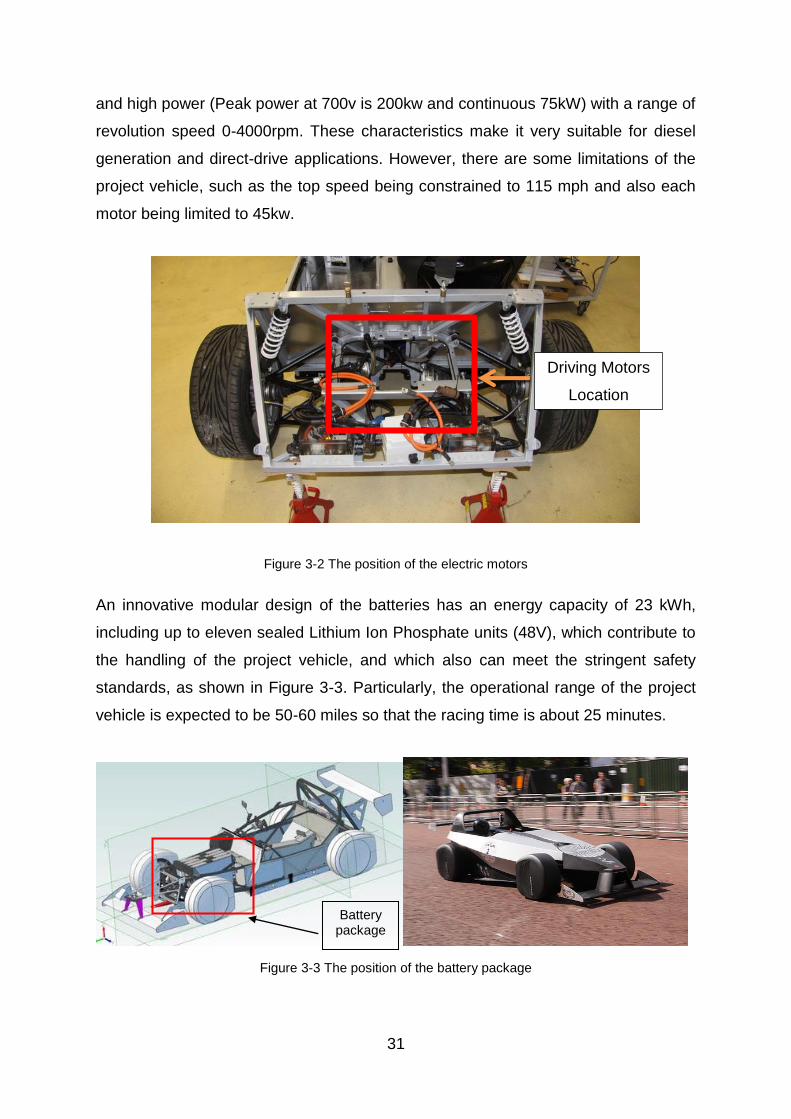
31

and high power (Peak power at 700v is 200kw and continuous 75kW) with a range of

revolution speed 0-4000rpm. These characteristics make it very suitable for diesel

generation and direct-drive applications. However, there are some limitations of the

project vehicle, such as the top speed being constrained to 115 mph and also each

motor being limited to 45kw.

Figure 3-2 The position of the electric motors

An innovative modular design of the batteries has an energy capacity of 23 kWh,

including up to eleven sealed Lithium Ion Phosphate units (48V), which contribute to

the handling of the project vehicle, and which also can meet the stringent safety

standards, as shown in Figure 3-3. Particularly, the operational range of the project

vehicle is expected to be 50-60 miles so that the racing time is about 25 minutes.

Figure 3-3 The position of the battery package

Battery package

Driving Motors

Location

32

3.2.2 Chassis and Suspension system

Westfield Sportcars have completed a ‘light-weighting‘ project working with tubing

specialist Reynolds Technology, creating a new car chassis and wishbone by

replacing much of the traditional mild steel with alloy tubing as used in Tour de

France race bicycles, as shown in Figure 3-4.

Figure 3-4 The pictures for the chassis and suspensions

The design team chose to reduce the weight of the chassis and the wishbones by

examining the possibility of using new thin-walled alloy tubing developed by

Reynolds in place of the mild steel tubes used previously, as shown in Figure 3-5.

a) Front b) Rear

Figure 3-5 The pictures of the front and rear suspensions

33

3.3 Modelling project vehicle

In this section, the main systems will be modelled and assembled in computing-

based software – ADAMS that can allow a number of vehicle subsystems to be

modelled and simulated, namely the driveline, chassis and vehicle body. The

modelling of a road as an element is also included to constitute the entire vehicle

model; and modelling the suspension system is the most important part in this

process.

The overall vehicle model is prepared using the Automated Dynamic Analysis of

Mechanical Systems (ADAMS) tool from MSC.Software. ADAMS is a widely used

tool for computing the large amplitude non-linear dynamic behaviour of systems such

as ground vehicles. For this exercise, the ADAMS/Car environment was not used in

order to make the modelling practices more transparent – the extensive use of

templates and ―sealed up‖ run-time procedures can sometimes make it difficult to

understand the exact performance of the model when using the ―Car‖ environment.

The process which has been used for modelling is planned to easily make some

modifications later in the design. So, using the graphical user interface of

ADAMS/View to create the full project vehicle as shown in Figure 3-6, the starting

point is to create hard points to indicate the different key locations of the subsystems.

As follows, these hard points are used to create the linkages; then the different joints

are added to connect the components together to finalize the system. Finally, all the

components of the project model have the mass and inertia properties.

Figure 3-6 Westfield i-Racer model in ADAMS/View

34

In the following section, a model audit is carried out so that it can ensure that the

model is more reliable and precise. More discussions are involved in this section and

the auditing aspects of the model are listed as below:

Sprung mass (The vehicle body)

Centre of Mass Position (The vehicle body)

Inertial Properties (All the components)

Un-sprung Mass

Spring and Damper Characteristics

Modal Solution

Total Degrees of freedom

Eigen Solution

3.3.1 Vehicle Body

The first concern for describing the full vehicle is to define the data set of the vehicle

body, namely the centre of mass position, the inertia properties and the masses, to

fulfil the requirements of the vehicle dynamics simulation. In this particular vehicle

model, the mass data of the vehicle body includes the mass of the body frame as

well as the additional masses of the Front Battery Module, Motors, Bracket, Coolant

and Controllers, and a passenger may even be added. Based on the project vehicle

with a conventional architecture, a summary of the main data collections will be

exhibited, namely that of the suspension geometry and the structure of the vehicle

body. The original geometric data was captured using a single point Faro arm

measuring device in the Coventry University Workshop, and all the dimensions of all

the systems such as the suspensions, the springs and dampers, and the body were

then processed using ADAMS to collate all of the data and achieve the single point

data, as required for the computer simulations.

The mass of the Westfield i-Racer model was measured in the Coventry University

Laboratory. It is important to note that the battery pack module, the complete rear

motor controller unit and the vehicle body panels, as additional masses to the mass

of the full vehicle, were assessed. The front, rear and full vertical loads are

measured so that the mass and the centre of mass position in the longitudinal are be

35

defined. Here is a method to attain the centre of mass height, which is to lift the rear

axle of the vehicle so the vehicle centreline from front to rear creates a certain angle.

A diagram of this is shown in Figure 3-7; reproduced with permission from Milliken.

Figure 3-7 The method for locating vehicle centre of mass height (Milliken, 1955)

The solution for vehicle height is given by equation (3.1).

(

)

(3.1)

This item has been removed due to third party copyright. The unabridged version of the thesis can be viewed at the Lanchester Library, Coventry University.

36

RL is the radius of the front tyre, W is the total weight of the vehicle, and WF is the

weight of the front of the vehicle during the test. The above method gave the centre

of mass height at 232 mm above the road surface. Using this approach, where the

total masses of the vehicle were the summation of the major components, the mass

centre position can also be found by using the method described above.

The inertia properties of the vehicle body need to be determined because the

dynamics of an actual vehicle are significantly affected by the yaw moment of

inertia . This data generated mainly focused on two main areas in the mass of the

chassis and four wheels. There is a detailed model to represent the mass and inertia

properties for the body that involves the overall masses of an approximate chassis,

battery Module and a motor controller which is provided by Westfield Sportcars, as

shown in Figure 3-3 above.

3.3.2 Suspension System

A completed suspension system as a most important system of the full vehicle model

will be established. In order to achieve a suspension model representing the one

installed on the actual vehicle, the use of powerful multi-body systems analysis

programs can be used. In the following discussion, modelling of a double wishbone

suspension system at both the front and rear of the vehicle is referred to as a

Linkage Model. Thus, the components of the suspension as rigid bodies can be

modelled in detail and the actual front and rear suspensions as shown in Figure 3-8.

Figure 3-8 The actual front and rear suspensions

37

The SAE coordinate system is used while modelling the vehicle, with x backward, y

to the right, and z downward. The origin is located directly below the centre of the

vehicle body geometry. SI units are used, i.e. metres for length, Newtons for force,

kilograms for mass and seconds for time. The data for the hard point locations are

measured by using a single point Faro arm-measuring device in the Coventry

University Laboratory. Table A5.1 lists the hard point coordinates of the right front

side suspensions hard points. The left side hard points are coded as mirror images

of the right points on the x-z plane. Hard-coding the left side as a mirror image of the

right makes it simpler to make changes in the suspension geometry, as changing the

coordinates of a point on the left side automatically maintains the symmetry of the

right side. Table A5.2 lists the hard point coordinates for the rear left suspension.

Here again the left side is hard coded as the mirror image of the left. The tables can

be found in Appendix 5.

The linkages of the suspension are generated by using the various shapes of the

rigid body in the Tool-box. The hard points were defined as being used to locate the

positions of each suspension linkage and to generate the completed suspension

geometry. The main components of the suspension are modelled separately and

linked to each other through the joints. Figure 3-9 shows the front and rear

suspension model in ADAMS/View. To clarity and simplify, the graphics of the

Westfield i-Racer body are modelled as a dummy part that has the same mass and

inertia properties as the body.

a) Front suspension model b) Rear suspension model

Figure 3-9 Front and rear suspension model in ADAMS/View

38

The Westfield i-Racer employs a double wishbone suspension on the front driving

axle and a deformed double wishbone suspension on the rear driving axle. For each

suspension, upper and lower A-shape arms and wheel knuckle are created as parts.

Bushings are used to connect the two A-shape control arms to the sub-frame, and

the control arms are linked to wheel knuckle by using spherical joints. The reason for

using the bushings there is to introduce some steering compliance, so that the

bushings as modelled have extremely high stiffness in the longitudinal and vertical

directions, and are comparatively soft in the lateral direction. Again, all the

components have their own mass and inertia properties.

The spring and damper configurations are created initially using the internal ADAMS

commands so that a spring damper unit can be generated automatically. The springs

are modelled by using a linear single component force that acting between the upper

and lower mounting points of the strut. The force is used to define by a constant

stiffness value with spring deflection. Westfield provided nonlinear damper data that

is modelled using a single component force acting between the same mounting

points as the spring. The nonlinear damping force is defined by a 2D curve with

deformation velocity along the x axis and force on the y axis as shown in Figure 3-10.

Figure 3-10 The 2D curve for the nonlinear damper

Velocity (mm/s)

Forc

e (

N)

39

The purpose of the software to model the suspension structure is now well

established and will be discussed further in the next chapter. The results from this

type of analysis are mainly geometric and allow the outputs to be plotted graphically,

such as the camber angle or roll centre position against the vertical wheel movement.

The double wishbone suspension model can be simplified to represent connecting

the A-shape control arms to the sub-frame. Modelling the suspension in this manner

is necessary to calculate the degrees of freedom (DOF) for both the front and rear

suspension systems.

Part 6 × 6 =36

Spherical 4 × -3 = -12

Revolute 2 × -5 = -10

Translation 1 × -5 = -5

Hook 2 × -4 = -8

ΣDOF = 1

Hence, the calculation as shown above is an example showing that the motions of all

six parts at the front suspension have been constrained by using different types of

joints, as shown in Figure 3-11. Note that the type of the joint has to be chosen

correctly in its location to attach the two parts together; otherwise the additional or

incorrect numbers of degrees of freedom may cause the suspension system failure,

or movement in the wrong direction. Also, the revolute joints that connected the

wishbones to the frame will be replaced by bushings when using the full vehicle

model for handling simulations.

40

Figure 3-11 The parts connected by the correct joints

3.3.3 Steering System

The configurations of the steering system based on linkages and steering gearboxes

are available for both cars and trucks. The steering system in the following sections

is modelled by using a conventional Rack-Pinion system. Modelling a steering

system on the actual vehicle can be represented as shown in Figure 3-12. Basically,

a cylinder is used to model the steering column connects to the vehicle body by

using the revolute joint, which the axis of the joint should align along the line of the

column. The motion or torque inputs of the steering control are applied at this

revolute joint to manoeuvre the vehicle model. Using a translational joint connecting

the steering rack to the vehicle body is represented, and the rack is linked to the tie

rods by using two universal joints. The steering ratio can be implemented into this

system by using a coupler statement that can convert the rotation of the steering

wheel inputs to the translation movement of the steering rack.

Revolute Joints

Spherical Joints

Universal

Joints

41

Figure 3-12 Modelling steering system in ADAMS

When starting the vehicle dynamics analysis, the steering ratio is always an

important parameter for the model design; the relationship between the turning the

steering hand wheel and the steer change at the front wheels has to be known. This

coupler is based on a ratio where one degree of the steering column input generates

the 0.18mm translational motion of the steering rack. This relationship is utilized to

connect the two tie rods at the front suspension, and then control the steer angle at

the wheels. Using a variable statement can measure out the steer angle of the front

wheels. A steering ratio can be determined by a common fashion, degree-to-degree,

which is the 22 degrees of hand wheel inputs relating to 1 degree of front wheel

steering, as shown in Figure 3-13. In both the linkage model and the real vehicle, the

steering ratio would vary when the wheels move in the motion of the full bump and

rebound, or the vehicle rolls.

42

Figure 3-13 The steering ratio for Westfield i-Racer model

3.3.4 Aerodynamic Effects

Some classic assessments of aerodynamics in existing text books (Milliken and

Milliken, 1995; Gillespie, 1992) that corresponds to the vehicle dynamics is

introduced. As is known, when the air flows through the vehicle body, forces and

moments can be produced because of the friction and pressure distribution between

the air and the body surface. Thus, the forces in the longitudinal, lateral and vertical

directions along with the moments in roll, pitch and yaw will arise in the same

reference frame as that of the vehicle body.

In this simulation, the project vehicle moves only in the plane so that it is going to

require at least the formulation of a longitudinal force , a lateral force . The

direction of the project vehicle will be changed during the manoeuvre, hence it is

going to be necessary to model the forces as components in the body-centred axis

system located at the mass centre. The magnitude of the aerodynamic forces can be

calculated out by using the equation 3-2 as shown below:

43

(3-2)

Where = the aerodynamic drag coefficient

= the density of air

= the frontal area of the vehicle

= the velocity of the vehicle in the direction of travel

Using this equation, there are only two forces that were applied within the model to

exert the effects on both the longitudinally and laterally direction of the vehicle. An

expected drag coefficient of 0.4 is used for the EV, and the rest of the data, such as

the frontal area of the vehicle, was included from the Westfield Sportcars. Figure 3-

14 shows that the aerodynamic drag forces act on the vehicle body when turning a

corner.

Figure 3-14 Aerodynamic drag forces in the lateral and longitudinal direction

Aero drag forces

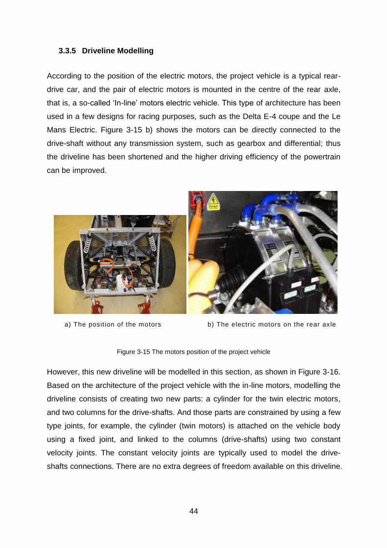
44

3.3.5 Driveline Modelling

According to the position of the electric motors, the project vehicle is a typical rear-

drive car, and the pair of electric motors is mounted in the centre of the rear axle,

that is, a so-called ‗In-line‘ motors electric vehicle. This type of architecture has been

used in a few designs for racing purposes, such as the Delta E-4 coupe and the Le

Mans Electric. Figure 3-15 b) shows the motors can be directly connected to the

drive-shaft without any transmission system, such as gearbox and differential; thus

the driveline has been shortened and the higher driving efficiency of the powertrain

can be improved.

a) The posit ion of the motors b) The electr ic motors on the rear axle

Figure 3-15 The motors position of the project vehicle

However, this new driveline will be modelled in this section, as shown in Figure 3-16.

Based on the architecture of the project vehicle with the in-line motors, modelling the

driveline consists of creating two new parts: a cylinder for the twin electric motors,

and two columns for the drive-shafts. And those parts are constrained by using a few

type joints, for example, the cylinder (twin motors) is attached on the vehicle body

using a fixed joint, and linked to the columns (drive-shafts) using two constant

velocity joints. The constant velocity joints are typically used to model the drive-

shafts connections. There are no extra degrees of freedom available on this driveline.

45

Figure 3-16 Modelling the driveline in ADAMS/View

There are some simulations required to retain the vehicle at a constant speed as in

the following studies, because if the vehicle does not have any form of the driving

torque, it will drive through the manoeuvres at a coasting condition using the

momentum available from the initial velocity. Furthermore, even ignoring the rolling

resistance and the aerodynamic drag force, the momentum of the vehicle will still

lose because of the resistant element of the cornering forces, which is generated at

the tyre during the manoeuvres. However, the means of modelling the driveline is to

implement the driving torques to the driven wheels, then produce the traction at the

contact patch; thus, the points for applying the driving torques on the driveline have

been chosen at the two cylindrical joints. It is more like a real vehicle driven with

electric motors, in which the torque generally outputs from the centric rotor of the

electric motor.

The rotation of the two rear wheels is coupled to the rotation of the rotors of the

electric motors, and the driving torque outputs are equally distributed to each of the

drive-shafts as 50% of the torque. It can be considered as an ‗open differential‘

mounted on the rear axle, which means the new driveline allows the rear wheel to

rotate at different speeds during cornering, but only by applying the same torque on

each of the driving wheels. Table 3-1 shows all bodies, joints and total DOFs have

Motors

Drive-shafts

Driving Torque

46

been calculated by using a function in ADAMS, confirming the model has 15 DOFS

and there are no redundant constraint equations.

Table 3-1 A list of all bodies, joints and DOFs

Before finishing this section to describe how to model the driveline, there is a method

that needs to be represented. Namely, the driving torque acted on the drive-shafts

can be modelled by using an existing TORQUE command in ADAMS/View. Thus,

the torque can be controlled by using a function or subroutine in the TORQUE

command that can be used to apply a control strategy for the vehicle dynamics or

stability control to the driveline. For example, if the model runs at a ‗drifting‘ condition,

the torques from the driveline are deactivated, and the driveline is also able to

produce equal torques on both the driving wheels to represent an ‗open differential‘.

It is a limitation of an open differential that the amount of total torque applied to both

drive wheels depends on the side with the least traction. For example, when one

wheel acts on a slippery surface, the torque applied to the other wheel would be the

same as that on the slippery side. Thus, the total torque could be reduced and may

be not enough for vehicle propulsion. In additional, the average of the rotational

speed of the two driven wheels equals the input rotational speed of the drive shaft,

and an increase in the speed of one wheel is balanced by a decrease in the speed of

47

the other. These characteristics can be represented by the function or subroutine

associated with the torque to improve the control strategy of the driveline.

Furthermore, even a more complex control strategy, such as torque vectoring control,

can exploit this approach to implement all the control concepts or requirements into

the driveline, and that will be discussed in Chapter 6.

3.4 Tyre modelling

The subject of extensive research, tyre modelling mainly focuses on how to model

the forces and moments generated at the contact patch where the tyres touch the

road surface. Pacejka and Sharp (1991) provided and developed the most common

tyre model, which have been broadly used, and the tyre model can compromise the

modelling of the tyres between the accuracy and complexity.

The research mainly focuses on a vehicle handling study, thus the project model is

generally manoeuvring on a flat road surface. In general, the tyre model is used to

create and model the forces and moments generating at the contact patch between

the tyre and the road surface. These forces and moments will transfer through the

suspension into the vehicle body. There are the three orthogonal forces and the

three orthogonal moments that can be calculated by the tyre model at each wheel

centre, controlling the vehicle body motion. Again, for the handling of the analysis,

the calculation of the tyre model is mainly based on the longitudinal direction (driving

and braking forces) and lateral forces, also including the formulation of rolling

resistance and aligning moments. A flat 2D road file is used as a part of the model;

furthermore it has the function to change the friction coefficient of the road surface to

represent the various surface textures, namely dry, wet and ice conditions.

3.4.1 Modelling virtual tyre rig

The aim of modelling the tyre test rig is to provide a tool to integrate a given tyre

model and its associated data set before using this with a vehicle simulation.

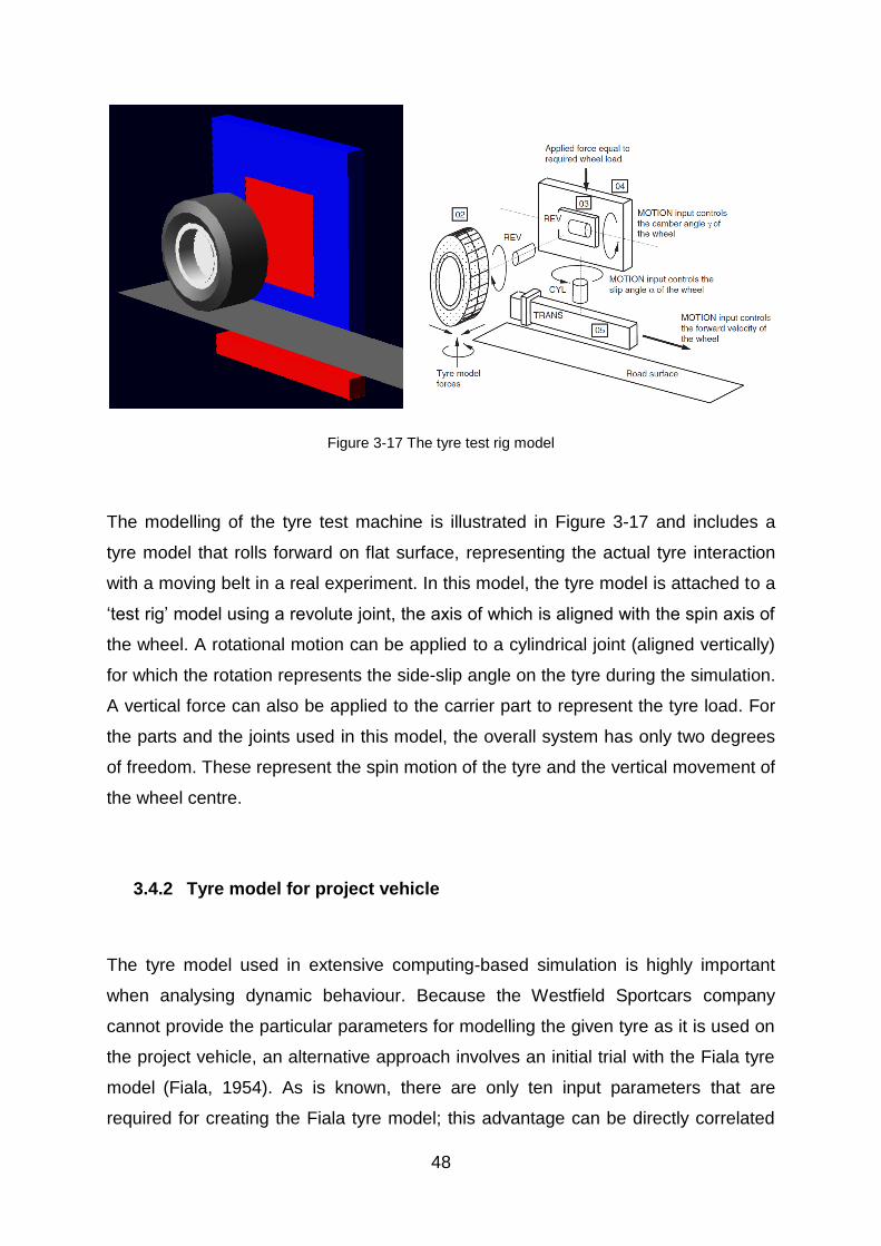
48

Figure 3-17 The tyre test rig model

The modelling of the tyre test machine is illustrated in Figure 3-17 and includes a

tyre model that rolls forward on flat surface, representing the actual tyre interaction

with a moving belt in a real experiment. In this model, the tyre model is attached to a

‗test rig‘ model using a revolute joint, the axis of which is aligned with the spin axis of

the wheel. A rotational motion can be applied to a cylindrical joint (aligned vertically)

for which the rotation represents the side-slip angle on the tyre during the simulation.

A vertical force can also be applied to the carrier part to represent the tyre load. For

the parts and the joints used in this model, the overall system has only two degrees

of freedom. These represent the spin motion of the tyre and the vertical movement of

the wheel centre.

3.4.2 Tyre model for project vehicle

The tyre model used in extensive computing-based simulation is highly important

when analysing dynamic behaviour. Because the Westfield Sportcars company

cannot provide the particular parameters for modelling the given tyre as it is used on

the project vehicle, an alternative approach involves an initial trial with the Fiala tyre

model (Fiala, 1954). As is known, there are only ten input parameters that are

required for creating the Fiala tyre model; this advantage can be directly correlated

49

to the characteristics of the tyre. Nevertheless, the major limitations of the tyre model

include the following: a) the model does not have the ability to represent the

combined situation, such as cornering and braking, or cornering and driving at the

same time. b) Lateral force and aligning moment cannot be calculated as having a

camber angle. c) When the tyre with the vertical load moves on the straight line, the

variety of the cornering stiffness is not modelled.

Another suitable alternative approach is established to fulfil the requirements of the

simulation. It is achieved by using the ‗Magic Formula‘ tyre model (Bakker et al. 1986,

1989), of which the ‗Magic Formula‘ tyre model is now most well-established, based

on the work by Pacejka (Pacejka and Bakker, 1993). This model is a ‗point follower‘

model, which uses an empirical mathematical form that can be shaped with a

relatively small number of parameters to fit more or less any measured tyre dataset.

The ―point follower‖ term refers to the fact that the tyre is idealized as a single point

of contact, which has aggregate forces and moments for the entire contact patch.

This is the way that data is recorded on a typical tyre test machine and is completely

suitable for smooth road handling calculations at low tyre slip angles. Because of the

absence in the particular coefficients of the tyre model for the project vehicle, a set of

standard data was used, as shown in Table 3-3. The coefficients need to be adjusted

in a reasonable region within which the results from testing the tyre model on the rig

can fulfil the expectations of this particular tyre model under the dynamic

manoeuvring. Then, the tyre model has been tested on the virtual tyre test rig in

ADAMS, and examination of the tyre results will be shown in the following section.

50

Table 3-1 A set data for tyre model

These coefficients of the tyre model will be used for all simulations in later Chapters.

For these simulations, the tyre model was steered in a region of the slip angle and

operated under four different vertical loads (1962N, 3924N, 5886N and 7848N). The

examination of the tyre results is shown in Figure 3-18 and Figure 3-19; the results

represent some curves for the lateral force and the self-aligning moment during the

changes of the tyre slip angle. The results show that the tyre performed in an

intended behaviour; nevertheless, the coefficients created in the tyre model were

only modified to an approximate level. Further validation of the coefficients is needed

to ensure that the data from the test rig model are as near the same as possible to

the actual tyre characteristics, which has to be taken into account when examining

all of the results generated from the simulations.

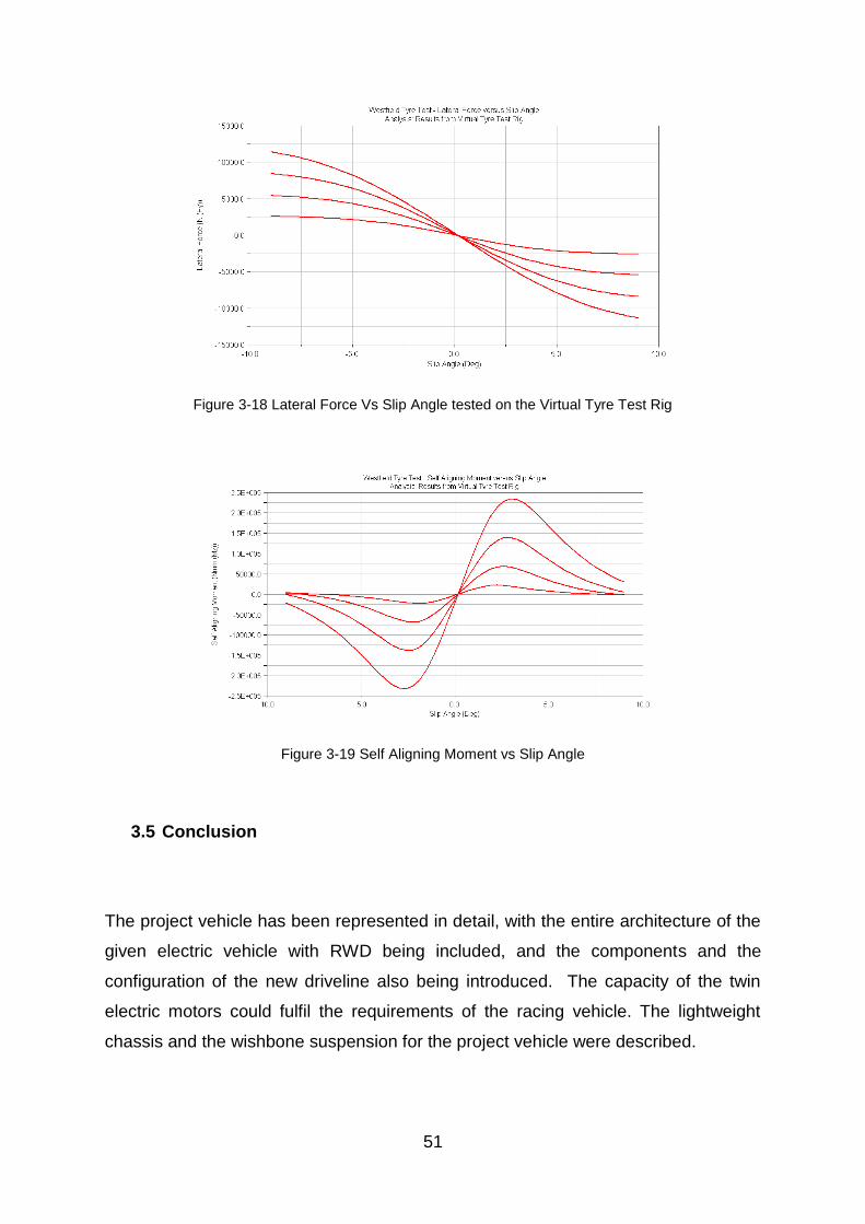
51

Figure 3-18 Lateral Force Vs Slip Angle tested on the Virtual Tyre Test Rig

Figure 3-19 Self Aligning Moment vs Slip Angle

3.5 Conclusion

The project vehicle has been represented in detail, with the entire architecture of the

given electric vehicle with RWD being included, and the components and the

configuration of the new driveline also being introduced. The capacity of the twin

electric motors could fulfil the requirements of the racing vehicle. The lightweight

chassis and the wishbone suspension for the project vehicle were described.

52

Several sub-systems of the vehicle, for example the vehicle body, the suspension

system and the driveline, have been modelled in ADAMS, and the audit was carried

out to ensure the reliability of the model. Also, the aerodynamic effects were

considered in this section. The driveline was able to produce the variable driving

torque at the wheels, so that it could represent the different driving modes, such as

the ‗open differential‘ and the torque vectoring control. The ‗Magic Formula‘ tyre

model was added on the vehicle model, and also used with the virtual test rig model

to examine characteristics of the tyre model in the intended behaviour due to

modifying the coefficients of the tyre model.

53

4 Measurement and analysis of the virtual model

4.1 Introduction

When building a vehicle model in a computer-based environment, the accuracy of

the simulation results relies on the accuracy of the model and the vehicle parameters

used to build the model. Hence, there are several methods available to validate the

vehicle model, such as kinematic studies and dynamic manoeuvres.

In order to verify the performance of the suspension system as modelled in Chapter

2, a range of characteristics will be determined through simulation of a quarter

vehicle model. In this chapter it will be shown that the full vehicle model will be

analysed in a number of ways that will provide information to support the following

investigations. Also, the steady-state cornering manoeuvre will be used to define the

basic driving characteristics of the vehicle model.

4.2 Kinematic analysis

The full vehicle model has been created in the previous chapter, where the

arrangement of the suspension system consists of the typical linkages for the

double-wishbone suspension to connect the wheels to the vehicle body. The

interaction of the linkages restricts the wheel plane to undergoing combined

translation and rotation. These motions are normally determined with respect to the

vehicle body, so the following descriptions will explain the kinematic analysis of the

wheel. For example, toe change for suspension linkages directly steers the front

wheels and generates lateral force and yaw moment. Camber angle is a

compensation angle to maintain the tyre perpendicular to the road surface when the

vehicle body rolls. Half-track change influences the lateral velocity of the tyre contact

patch via the roll rate. Hence, the slip angle of the tyre is affected, since the angle is

defined as the arctangent of the lateral and longitudinal velocities; an increase in the

lateral velocity directly increases the slip angle.

54

4.2.1 Quarter vehicle modelling

In this section, the basic function of the suspension system is represented from a

functional perspective. The front suspension of the vehicle model has been built as

one of the best-known suspension types, the so called ‗Double Wishbone system‘,

and also the double wishbone system has been created for the rear suspension.

Using the software to analyse suspension geometry is now well established and will

be discussed further in the next section of this chapter. The output from this type of

analysis is mainly geometric and allows results such as the camber angle to be

plotted graphically against the vertical wheel movement.

Modelling the quarter vehicle is discussed by using the existing double wishbone

suspension system at the front axle. Basically, the suspension model uses the

revolute joints to connect the upper and lower A-shape arms to the chassis as shown

in Figure 4-1. Imparting a vertical motion to the suspension is achieved through a

jack part that connects to the ground using a translational joint. Therefore, at the

translational joint the applied motion moves the jack through a range of vertical

movements that assumes the suspension moving between the bump and rebound

positions. An in-plane joint is applied to link the jack to the wheel knuckle where the

wheel centre is located. In addition, this joint only constrains the wheel centre at the

top of the jack to move in the plane, but the wheel can still rotate or move in the

lateral and longitudinal directions.

Figure 4-1 Modelling the front of the quarter project vehicle

55

Note that the resulting system model has a total of zero degrees of freedom. The

movement in the system is due to the introduction of a user prescribed time

dependant motion that accounts for one degree of freedom constrained from the

system. The resulting analysis is kinematic. The introduction of one or more

additional degrees of freedom would result in a dynamic analysis.

4.2.2 General approach for kinematic analysis

For a suspension system, the main function of a multi-body systems model is to

simulate the geometric position and orientation when the suspension has a vertical

movement between the full bump and full rebound positions (Blundell, 2004). When

simulating the vertical motion, the output is only suitable for a kinematic or quasi-

static analysis. As mentioned, the motion applied to the translational joint moves the

wheel between the 60mm rebound and 60mm bump positions. This results in

particular times for the movement, at 0.25 second for bump and at 0.75 second for

rebound, which enables the present of the continuous and smooth animation of the

movement cycles. The duration of the simulation time is 1 second with 100 output

steps, which ensures the results are calculated over the full bump and rebound

range. In ADAMS, a motion statement was used to move the translational joint

during all the simulations.

The motion statement is shown below, where the total movement between bump and

rebound is 120mm:

56

a) Front suspension b) Rear suspension

Figure 4-2 Kinematic simulation for suspension system

Something needs to be clarified at this stage in which the variable converts the time

in seconds to degrees in the function that represent one cycle over 1 second during

the simulation time. If implementing an asymmetric movement which involves

different distances in the bump and rebound, the motion input needs a more complex

function to operate in ADAMS.

4.2.3 Suspension measurements

Since ADAMS/View is general purpose multi-body dynamics simulation software, it

does not have any specialized tools to measure the various vehicle parameters that

need to be monitored and recorded to compare the performance of the vehicle.

Hence the different variables to measure and monitor various parameters such as

steering angle, camber angle and roll angle are created. The descriptions provided

here will be limited to the most commonly calculated outputs. The outputs shown in

Appendix 5 are for those plots that are normally used to compare simulation results

with physical test data for validation of the virtual model in ADAMS.

Bump Movement: Measuring the wheel movement upwards in the positive

vertical direction relative to the vehicle body.

Wheel Recession: Measuring the wheel movement rearwards in the positive

longitudinal direction relative to the vehicle body.

57

Half-Track Change: Measuring the wheel movement outwards in the positive lateral

direction relative to the vehicle body. All of these are shown in

Figure 4-3

Figure 4-3. A model diagram for the WR, HTC and BM (Blundell. 2004)

Camber angle: This measurement uses two markers that are positioned at the

wheel knuckle. The first marker (angle_wc) is situated at the

wheel centre on the knuckle, and the second marker (angle_sa) is

positioned on the axis of rotation of the wheel. The measure is

defined in ADAMS by the equation as shown in Figure 4-4:

Wheel Steer Angle: The road wheel steer angle is calculated using the same

markers used to measure the camber angle. The steer angle

measure is defined by the equation as shown in Figure 4-4:

This item has been removed due to third party copyright. The unabridged version of the thesis can be viewed at the Lanchester Library, Coventry University.

58

Figure 4-4. A diagram shows camber angle and steer angle

Castor Angle: The measurement of the castor angle is in degrees in the side

elevation between the vertical and the steering axis. The points for

measurement are located at the upper and lower ball joints of the

suspension system connect. Thus, the angle is defined by the

equation as shown in Figure 4-5:

Suspension Trail: The suspension trail is the length in the longitudinal direction

between intersection of the steering axis and the ground, and the

wheel base which can be described as below:

59

Figure 4-5. Calculation of castor angle and suspension trail

Steer Axis Inclination: The steer axis inclination is that the angle is measured at the

front elevation between the vertical and the steering axis

(from the upper ball joint to the lower ball joint). It can be

explained by the equation below (see Figure 4-6):

Ground Level Offset: The ground level offset is the length in the lateral direction

between intersection of the steering axis and the ground,

and the wheel base (see Figure 4-6):

Figure 4-6 Calculation of steering axis inclination and ground level offset

60

4.3 Dynamic analysis

In the automotive industry, there is considerable focus on ride and handling where

multi-body systems analysis is deployed to support design and analysis work. There

are multiple sources of ride vibration which generally fall into two areas, namely road

roughness and on-board sources. For vehicle dynamic analysis, the best starting

point is to know the basic properties of a vehicle and its suspension system i.e. the

motions of the body and axles. The body as a portion of the vehicle moves as an

integral unit on the suspension. The suspension and wheels, as the un-sprung

masses, move as a rigid body and impose excitation forces on the sprung mass.

Thus, one must look into structural modes of vibration and resonances of the sub-

system on the vehicle.

Before starting the computer-based simulation for dynamic analysis, manual

calculations are necessary to introduce how to find the natural frequencies of the

vehicle body and un-sprung between the suspension spring and the tyre spring. A

quarter vehicle model with two degrees of freedom and the data to support the

calculations is shown in Figure 4-7.

Figure 4-7 Two degrees of freedom quarter vehicle model (Blundell, 2004)

The un-damped natural frequencies for the body and for the un-sprung mass

can be estimated using the following equations. Note that for the body an equivalent

stiffness is determined to represent the combined contribution of the road and tyre

springs:

This item has been removed due to third party copyright. The unabridged version of the thesis can be viewed at the

Lanchester Library, Coventry University.

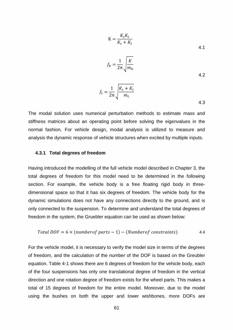
61

4.1

√

4.2

√

4.3

The modal solution uses numerical perturbation methods to estimate mass and

stiffness matrices about an operating point before solving the eigenvalues in the

normal fashion. For vehicle design, modal analysis is utilized to measure and

analysis the dynamic response of vehicle structures when excited by multiple inputs.

4.3.1 Total degrees of freedom

Having introduced the modelling of the full vehicle model described in Chapter 3, the

total degrees of freedom for this model need to be determined in the following

section. For example, the vehicle body is a free floating rigid body in three-

dimensional space so that it has six degrees of freedom. The vehicle body for the

dynamic simulations does not have any connections directly to the ground, and is

only connected to the suspension. To determine and understand the total degrees of

freedom in the system, the Gruebler equation can be used as shown below:

4.4

For the vehicle model, it is necessary to verify the model size in terms of the degrees

of freedom, and the calculation of the number of the DOF is based on the Greubler

equation. Table 4-1 shows there are 6 degrees of freedom for the vehicle body, each

of the four suspensions has only one translational degree of freedom in the vertical

direction and one rotation degree of freedom exists for the wheel parts. This makes a

total of 15 degrees of freedom for the entire model. Moreover, due to the model

using the bushes on both the upper and lower wishbones, more DOFs are

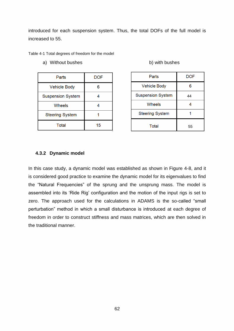
62

introduced for each suspension system. Thus, the total DOFs of the full model is

increased to 55.

Table 4-1 Total degrees of freedom for the model

a) Without bushes b) with bushes

4.3.2 Dynamic model

In this case study, a dynamic model was established as shown in Figure 4-8, and it

is considered good practice to examine the dynamic model for its eigenvalues to find

the ―Natural Frequencies‖ of the sprung and the unsprung mass. The model is

assembled into its ‗Ride Rig‘ configuration and the motion of the input rigs is set to

zero. The approach used for the calculations in ADAMS is the so-called ―small

perturbation‖ method in which a small disturbance is introduced at each degree of

freedom in order to construct stiffness and mass matrices, which are then solved in

the traditional manner.

44

55

63

Figure 4-3 The dynamic model for modal solution

The dynamic model is essentially a basic version of the full vehicle model which only

includes the suspension system and the vehicle body, thus reducing the total DOF to

10. The four tyres are replaced by a single spring unit that has the same stiffness as

the tyre, and in-plane joints are added between the spring unit and the ground part to

ensure that the unit is perpendicular to the ground, and also includes a planer

constraint ( direction) on the ground. The simulation runs in the dynamic mode for

two seconds and examines the vehicle model to find the natural frequencies for each

degree of freedom.

The results are shown in Table 4-2. The information includes: the sequential number

of the mode that is predicted by the Eigen solution, natural frequencies

corresponding to the modes, damping ratios for the modes and list the real and

imaginary parts of the eigenvalue. The table of results from ADAMS/View produces

ten modes of vibration for this full linkage vehicle model, and also includes the total

number of the parts and the joints. Finally, the model is verified to show there are ten

degrees of freedom for the model and no redundant constraint equations.

64

Table 4-2 Display of the eigenvalues in tabular form

The calculation for eigenvalues and eigenvectors can be done by using a function of

ADAMS which can give a better understanding of the model‘s natural frequencies

and mode shapes. After the calculation is complete, ADAMS can display in tabular

form the Eigenvalues, in which the particular stability behaviour of the model

depends on the existing real and imaginary parts of the eigenvalues, and the signs of

the real parts and the different values of both parts. However, the model is a stable

system in which all the real values are negative and the system has an imaginary

part in which one pair of the values corresponds to each mode. In addition, each of

the natural frequencies corresponds to the mode shapes that are the deformations of

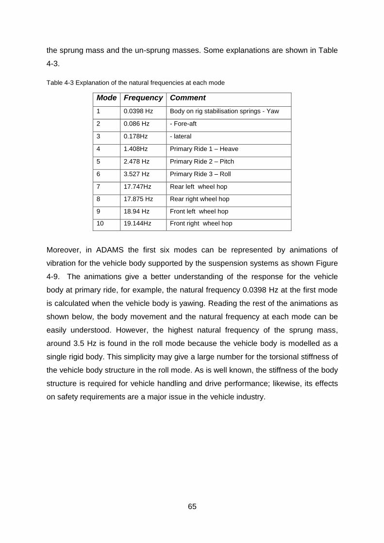
65

the sprung mass and the un-sprung masses. Some explanations are shown in Table

4-3.

Table 4-3 Explanation of the natural frequencies at each mode

Mode Frequency Comment

1 0.0398 Hz Body on rig stabilisation springs - Yaw

2 0.086 Hz - Fore-aft

3 0.178Hz - lateral

4 1.408Hz Primary Ride 1 – Heave

5 2.478 Hz Primary Ride 2 – Pitch

6 3.527 Hz Primary Ride 3 – Roll

7 17.747Hz Rear left wheel hop

8 17.875 Hz Rear right wheel hop

9 18.94 Hz Front left wheel hop

10 19.144Hz Front right wheel hop

Moreover, in ADAMS the first six modes can be represented by animations of

vibration for the vehicle body supported by the suspension systems as shown Figure

4-9. The animations give a better understanding of the response for the vehicle

body at primary ride, for example, the natural frequency 0.0398 Hz at the first mode

is calculated when the vehicle body is yawing. Reading the rest of the animations as

shown below, the body movement and the natural frequency at each mode can be

easily understood. However, the highest natural frequency of the sprung mass,

around 3.5 Hz is found in the roll mode because the vehicle body is modelled as a

single rigid body. This simplicity may give a large number for the torsional stiffness of

the vehicle body structure in the roll mode. As is well known, the stiffness of the body

structure is required for vehicle handling and drive performance; likewise, its effects

on safety requirements are a major issue in the vehicle industry.

66

a) Mode_1 Yaw b) Mode 2 Fore-aft

c) Mode 3 Lateral d) Mode 4 Heave

e) Mode 5 Pitch f) Mode 6 Roll

Figure 4-4 Animations of the modes at primary ride behaviour

67

In this model, the suspensions and the rigs are the un-sprung mass of the vehicle

that is the second largest of the masses. In general, all un-sprung masses have the

vertical hop mode that is excited by the road uneven inputs adding to the vibrations

present on the vehicle. Thus, the four-wheel hop modes are sensibly positioned with

respect to each other, and are represented in Figure 4-10. It can be seen that the

natural frequencies are much higher than the sprung mass resonance, so that the

sprung mass remains stationary during the wheel hop.

a) Wheel hop - Rear left b) Wheel hop – Rear right

c) Wheel hop – Front left b) wheel hop – Front right

Figure 4-10 Animations of the modes at wheel hop behaviour

68

For a normal driving vehicle, the calculated frequency will be approximately 10 Hz.

Friction in the suspension will increase the effective spring rate for small ride motions

which in turn will increase the frequency to 12-15Hz. However, the wheel hop

frequencies are high compared to those of the normal passenger car due to the

track-racing nature of the vehicle, which means the vertical tyre stiffness and spring

damper face are comparatively high, raising the wheel hop mode frequency. The

purpose of kinematic and ride calculations are to check the virtual model has been

built correctly using a Multi-body system for following analysis, i.e. the correct

numbers of parts and the types of joints are being used in the model. Overall, the

model behaves well dynamically and can be trusted for its intended 0-20Hz dynamic

use in a numerical sense. However, in terms of representing real vehicle behaviour

there is one important caveat – the roll stiffness distribution as modelled may be very

different to the real roll stiffness distribution due to vehicle frame flexibility, about

which no information was available.

4.4 Steady-State Handling analysis

The classical treatment of the behaviour of the vehicle model, that is called steady

state cornering, is described out in this section. Steady state means the vehicle

states are unchanging with time and speed as the vehicle travels on a constant

radius circle. This treatment will be described in more detail; running the model

around a circle with constant radius at a range of constant speeds, the increments in

the speed should correspond to the increments in the lateral acceleration. Moreover,

this approach is very practicable to perform and so it will be used for the basis of

vehicle dynamic analysis in the following discussion.

4.4.1 Driver behaviour modelling – a ‘path following’ controller

Before starting the treatment, the first consideration of modelling the steering inputs

is to represent the driver as part of the full vehicle system model. In this research,

69

the inputs to the steering wheel are designed with both open-loop and closed-loop

control. The steering input with the open-loop control requires a time-dependent

rotation that will be applied to the steering system. If applying a closed-loop control

to the steering system, the aim is to adjust the input to produce the desired trajectory.

However, the aim of the control method is to minimize the error that is the difference

between the actual output and the desired output. In the literature, there are a variety

of controller models suitable for modelling driver behaviour in existence. Some, such

as ADAMS/Driver™ developed as part of the MSC.ADAMS modelling package, are

very complete – others, such as the two-loop feedback control model are simpler

(Blundell and Harty, 2004). Some researchers prefer to use a preview distance for

controlling the trajectory of the vehicle, with an error of lateral deviation from the

intended path. However, there is usually a difficulty associated with this since the

lateral direction must be defined with respect to the vehicle. For ‗normal‘ driving this

type of model can produce acceptable results but for manoeuvres such as the ISO

3888 Lane Change the behaviour becomes unacceptably oscillatory particularly after

the manoeuvre. An alternative method, used by the authors with some success for a

variety of extreme manoeuvres, is to focus on the behaviour of the front axle. This

model fits with driver‘s experience of driving at or near the handling limit, particularly

on surfaces such as snow where large body slip angles highlight the mechanisms

used in the driver‘s mind.

Ground Plane Velocity

The ‗path following‘ controller model focuses on the behaviour of the front axle in

which the principle of the control method is to determine the yaw rate error between

the ‗No-slip yaw rate‘ of the front axle and demanded yaw rate. The demanded yaw

rate is the driver controlling the vehicle to follow the path as expected at a range of

speed. The formulation used is described below. All subscripts x and y are in the

vehicle reference frame.

In Figure 4-11, the ground plan velocity Vg is the given from the components and

using

70

√

4.5

Figure 4-115 Explanation of Ground Plane Velocity

For the reference frame used here and as the vehicle moves forward, the signs of

and are negative. A variable command is used to calculate within the model to

find out what the significance of the ground plane velocity is. The units of model work

in and will be set up in . As the simplest start, the model will run for the

steady state cornering, the driving torques will not act on this model and it only has

an initial velocity on all parts, assuming the vehicle is in a coasting condition.

Demanded Yaw Rate

The demanded yaw rate d is found from the forward velocity and path curvature

using:

4.6

4.7

71

Figure 4-12 Explanation of Demanded Yaw Rate

For example, if the model runs at a 33m constant radius circle as shown in Figure 4-

12, the path curvature is = 0.0303m-1. So the demanded yaw rate can be easily

calculated depending on the ground plane velocity of the model.

Path curvature and path length

The path curvature for a circle should be a constant value, but it needs some

transition curves with varied radiuses to link path curvature from the straight line to

the constant radius circle. This approach can avoid abrupt steering inputs while the

vehicle model follows the desired path. The desired path curvature can be converted

to a SPLINE command as used in ADAMS, shown in Figure 4-13. The X values are

path lengths depending on vehicle speed, and Y values are path curvatures. Note

that the value of the path curvature can be positive or negative, so it needs some

definitions before the simulation. In this cornering scenario, when the path curvature

is set up for a positive value the vehicle model turns to the left and the negative

value makes the model turn to the right.

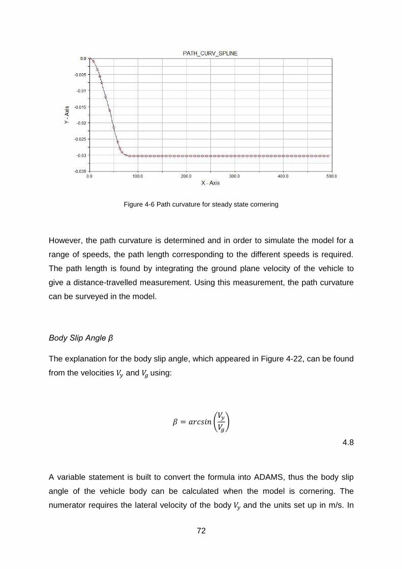
72

Figure 4-6 Path curvature for steady state cornering

However, the path curvature is determined and in order to simulate the model for a

range of speeds, the path length corresponding to the different speeds is required.

The path length is found by integrating the ground plane velocity of the vehicle to

give a distance-travelled measurement. Using this measurement, the path curvature

can be surveyed in the model.

Body Slip Angle β

The explanation for the body slip angle, which appeared in Figure 4-22, can be found

from the velocities and using:

(

)

4.8

A variable statement is built to convert the formula into ADAMS, thus the body slip

angle of the vehicle body can be calculated when the model is cornering. The

numerator requires the lateral velocity of the body and the units set up in m/s. In

73

order to avoid having the denominator equal to zero, a correction factor has been

added into the variable statement that can avert any the numerical failure. The effect

of the factor is negligible.

Centripetal Acceleration

First, the variables of lateral acceleration and longitudinal acceleration are

created and calculated in the vehicle body axis system, the units set up in m/s2.

Then, the centripetal acceleration is found from the components of acceleration

and using

4.9

The Front Axle No-Slip Yaw Rate

The front axle no-slip yaw rate ωfNs is found from the components of the centripetal

acceleration , the yaw acceleration , the distance , from the mass centre to the

front axle and the ground plane velocity using

4.10

Yaw rate error

The yaw rate error is then found from the demanded yaw rate and the front

axle no-slip yaw rate using

4.11

74

4.4.2 Driver behaviour modelling – a ‘survey’ controller

Before building the ‗survey‘ controller, some basic knowledge of the vehicle driving

characteristics during cornering needs to be mentioned. At the lowest speed, the

performance of the actual vehicle corresponds very closely with the geometric yaw

rate of the vehicle body. As vehicle speed rises, the lateral acceleration of the

vehicle is increased so that the tyres must develop lateral forces, and slip angles are

presented at each wheel. Due to the frictional limitations of the tyres, the vehicle

cannot reach the geometric yaw rate for a large steering input. Thus, the

characteristics of the vehicle are designed to have further modifications in which the

yaw rate gain should be reduced even when the tyres are not saturated. Therefore,

the over- or under-steer can be easily defined by the ratio of the geometric yaw rate

and the actual yaw rate, i.e. if the ratio is greater than one, the vehicle is under-

steering and when the vehicle is over-steering, the ratio is less than one,.

As is known, the tyre cornering force curve is treated as having linear, transitional

and frictional regions, and the project racing model may operate in all of these

regions. At the starting point, the response of the vehicle related to the driver control

will be operated in the linear region, corresponding to the lateral acceleration of the

vehicle body, which is about 0.3g (Milliken, 1995). Thus, a similar control method as

the path-following controller is used in the survey controller model in which only the

target behaviour differs slightly. The survey controller model still focuses on the

behaviour of the front axle, but the aim is to control the lateral acceleration of the

model at its linear region. Therefore, the target is set up for the body lateral

acceleration at 0.3g so that it can be converted into ADAMS by using the SPLINE

command. The SPLINE command represents the Y axis as target lateral

acceleration depending on the X values – for simulation time, and the units are

converted in m. Finally, the lateral acceleration can be found by using:

4.12

75

4.4.3 Steering torque input

The closed-loop driver model with the ‗Path Following‘ and ‗Survey‘ controllers will

be applied to the vehicle model by using a typical PID controller. As one of the

control technologies represented in the literature, the PID controller has the

advantage by which it produces continuous output and there are no steps that are

quite like the behaviour of a real driver. For example, when using the driver model

with the path-following controller, the yaw rate error is minimized in three ways: a

control effort is applied in proportion to the error, and then the error can be integrated

and also differentiated. In the PID formulation, the integral and derivative terms can

be represented by using DIF statements and variables in ADAMS. The controller

theory section for Yaw Rate Error (YRE) is shown below

∫

4.13

As stated, the simple steering system as modelled in the previous Chapter is using

the steering rack connecting the steering column and the tie rods of the front

suspension. The rotational motion of the steering column is related to the

translational motion of the steering rack through the coupler joint. This coupler is

based on a ratio where a degree of the steering column input generates the 0.18mm

translational motion of the steering rack. Therefore, the implementation of the control,

as shown in Figure 4-28 is to apply the torque to the steering column and the ‗driving‘

of the vehicle model follows the desired path.

76

Figure 4-7 Steering torque acting on steering wheel

When the driver model implements the control signal on the steering wheel, the PID

controller can modify the steering torque to minimize the yaw rate error. This is more

like the behaviour of a real driver because when the yaw rate error increases the

driver will apply more torque on the steering wheel to reduce the error and keep the

vehicle on track. The SFORCE statement in ADAMS is used for implementation of

the steering torque input as shown in Figure 4-29.

Figure 4-8 Steering input for the ‗path following‘ model

77

4.5 Simulation results

4.5.1 Steady state cornering behaviour

The cornering behaviour of a vehicle is an important performance attribute that

normally corresponds to the handling. There are three phases when a vehicle makes

a turn into a corner, turn entry, steady-state cornering and turn exit. During the

second phase, the radius of the path and velocity of the vehicle are constant. The

Ackermann angle which is the average steer angle of the wheels, δ=L/R, can be

found.

In the general steady state cornering manoeuvre, it is necessary to consider the

relationships in Figure 4-30. The under-steer region requires more steer angle than

the Ackermann angle to drive the vehicle in the desired circle. Similarly, the over-

steer region has less steer angle compared to the Ackermann angle.

Figure 4-9 The explanation of Under-steer or Over-steer (Gillespie, 1992)

To determine the characteristics of the project vehicle, such as under-steer or over-

steer, the constant radius turn test procedure, which is based on the British standard

(ISO 4138), can be used. The procedure may be summarized as follows: for the first

step, the model starts running at low speed to find the Ackermann angle

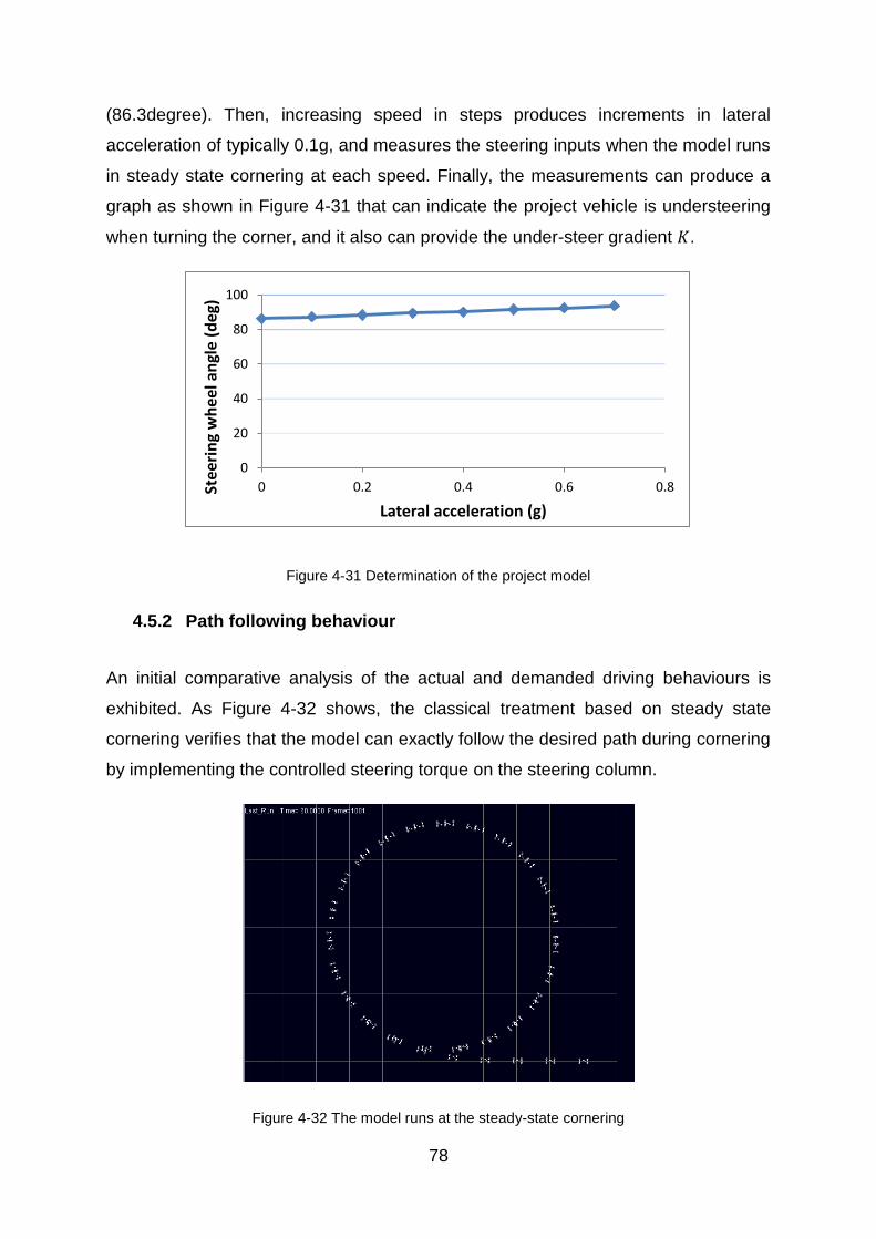
78

(86.3degree). Then, increasing speed in steps produces increments in lateral

acceleration of typically 0.1g, and measures the steering inputs when the model runs

in steady state cornering at each speed. Finally, the measurements can produce a

graph as shown in Figure 4-31 that can indicate the project vehicle is understeering

when turning the corner, and it also can provide the under-steer gradient .

Figure 4-31 Determination of the project model

4.5.2 Path following behaviour

An initial comparative analysis of the actual and demanded driving behaviours is

exhibited. As Figure 4-32 shows, the classical treatment based on steady state

cornering verifies that the model can exactly follow the desired path during cornering

by implementing the controlled steering torque on the steering column.

Figure 4-32 The model runs at the steady-state cornering

0

20

40

60

80

100

0 0.2 0.4 0.6 0.8Stee

rin

g w

hee

l an

gle

(de

g)

Lateral acceleration (g)

79

Moreover, the implementation of the closed-loop driver control with the PID controller

provides the adjustable steering torques so that the yaw rate error can be minimized

as shown in Figure 4-33.

Figure 4-10 Demanded Yaw Rate Vs Front Axle No-Slip Yaw Rate

4.5.3 Vehicle linearity

In a process similar to that for the driver model with ‗path following‘ controller, the

‗survey‘ controller operates the vehicle model running at its linear region as shown in

Figure 4-34. The linear steady-state control response characteristics are given as a

series of ratios: curvature response, yawing velocity response and lateral

acceleration response. As mentioned, the reason for steering the vehicle is to

change the direction of the vehicle by developing the yaw rate. Thus, the notion of

yaw rate gain which is a ratio of yaw rate to steer angle at the front wheels, becomes

useful to describe the yaw velocity response to control inputs.

80

Figure 4-11 The vehicle lateral acceleration versus target lateral acceleration

Again, for vehicle stability and control, the basic characteristics of the vehicle need to

be considered. If the response of the vehicle is less than what might have been

expected, the term understeer is used. When the vehicle yaws more than expected,

the term oversteer is used – the response of the vehicle exceeding what might have

been expected. So far the approach for measuring the steering inputs to define the

under- or oversteer has been discussed. Remaining with Newtonian friction to

describe the behaviour of the tyres, one further fundamental point is worth

establishing, which is the relationship between the yaw rate gains with forward

velocity as shown in Figure 4-36. When the model is at low speed, the yaw rate gain

is very close to the ideal yaw rate gain value, which means the response of the

vehicle control is more like that of a natural steer vehicle. When the vehicle speed

increases, the vehicle is unable to achieve the ideal yaw rate for large steering

angles. The characteristics of the vehicle are performed to further reduce the yaw

rate gain even when the tyres are not saturated. Furthermore, based on the vehicle

characteristics, an authority envelope of torque vectoring control is carried out in

Figure 4-36, so that the aim for the torque vectoring control which will be developed

in this research is to control the vehicle behaviour close to its own characteristics

when running at various conditions.

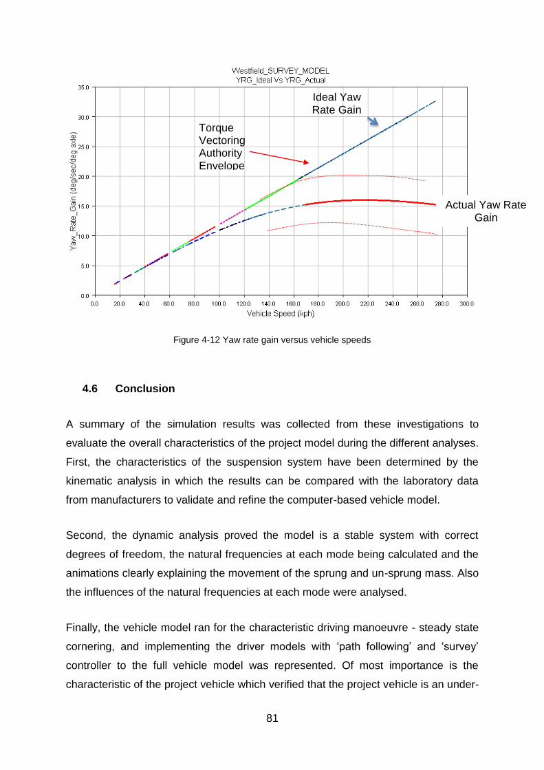
81

Figure 4-12 Yaw rate gain versus vehicle speeds

4.6 Conclusion

A summary of the simulation results was collected from these investigations to

evaluate the overall characteristics of the project model during the different analyses.

First, the characteristics of the suspension system have been determined by the

kinematic analysis in which the results can be compared with the laboratory data

from manufacturers to validate and refine the computer-based vehicle model.

Second, the dynamic analysis proved the model is a stable system with correct

degrees of freedom, the natural frequencies at each mode being calculated and the

animations clearly explaining the movement of the sprung and un-sprung mass. Also

the influences of the natural frequencies at each mode were analysed.

Finally, the vehicle model ran for the characteristic driving manoeuvre - steady state

cornering, and implementing the driver models with ‗path following‘ and ‗survey‘

controller to the full vehicle model was represented. Of most importance is the

characteristic of the project vehicle which verified that the project vehicle is an under-

Torque Vectoring Authority Envelope

Ideal Yaw Rate Gain

Actual Yaw Rate Gain

82

steer vehicle. Furthermore, Figure 4-23 for the yaw rate gain against the vehicle

speed indicated that the aim of the further control strategy for active yaw control is to

overcome all the variations, and then to dominate the vehicle running at its particular

characteristics.

83

5. Comparison of architecture for electric vehicle

5.1 Introduction

For conventional vehicles, a main difference in architecture is the position of the

Internal Combustion (IC) engine which can be located at the front, middle or rear of

the vehicle. The type of mechanical driveline also is another important factor of

vehicle architecture, such as Rear Wheel Drive (RWD) or All Wheel Drive (AWD). A

novel architecture for electric vehicle driveline was a design that includes freedom to

move the motors to a particular space in the vehicle, for example, mounting the

motors within individual wheels. In addition, the electric motors can also be located in

the middle of the chassis at the front, rear or both axles.

In recent year, the architecture of electric vehicle with in-wheel motors on the market

has high driving efficiency, thus any other architecture may be neglected. Westfield

Sportcars, a producer of in-line motors, has recommended a series of wide-ranging

studies into the vehicle stability and driveability performances. Therefore, a

comparison will be discussed in this chapter that includes ride comfort check and

drivability check by using the ADAMS model. The discussion can provide a

comprehensive overview of using in-wheel and in-line motors in this particular racing

model.

5.2 Architecture of in-wheel motors vehicle

The change in the un-sprung mass significantly affects the ride and handling

behaviour thus it is an important parameter. Many feasibility researches have been

done broadly for in-wheel motors, some specific and detailed measures for the sizes

of the effects in dynamics behaviours have been taken. The ride and handling

performance from subjective and objective measures suggests that the modern

development toolbox is easily capable of restoring dynamic performance. However,

the advantages of the in-wheel motors in terms of packaging and vehicle dynamics

control are of substantial interest to the vehicle dynamics community (Anderson and

Harty 2010).

84

In recent years, a popular novel architecture of electric vehicle has developed by

using electric motors mounted in driving wheel hubs that is effective in reducing the

components of the entire traditional drivetrain. The higher driving efficiency of the

powertrain can be improved which the fuel tank to wheel efficiency of the

conventional powertrain is about 20% (Göschel and Burkhard, 2008), that of an

electric vehicle with in-wheel motors amounts approximately 80% (Neudorfer, H and

Binder, A, 2006).

Some new designs of suspension system with in wheel motor were published in last

decades. First, Willberger and Ackerl (2010) designed an elementary model of

intergraded suspension with in wheel motor as shown in Figure 5-1, which consisted

of an electric motor, gear box and brake system. Eduardo and Rojas (2011)

developed a single wheel suspension system to integrate entire demanded

components together. The integration mainly considers in two aspects: first, if an

electric motor will be integrated into an existing suspension system, the effect on the

behaviour of the characteristic suspension parameters has to be minimized during

the adjustment should reach the target behaviours of the vehicle handling. Moreover,

it enables preventing any impact between suspension elements and the in-wheel

motor. The modification bases on an original rear axle of Ford Focus 1999

suspension system, as mentioned, an electric motor and a gearbox are equipped

into the wheel hub as the practical application example.

(a) (b)

Figure 5-1 Different design of in-wheel motors

Optimized suspension system for passenger vehicles with in-wheel

motors (Eduardo and Rojas, 2011)

Package design: 1. Electirc motor 2. Gearbox 3. Brake

disc 4. Suspension arm (Willberger and Ackerl , 2010)

85

There are several different types of in-wheel motors in the literature mainly used for

either pure and hybrid electric propulsion units in vehicles. The aim is to satisfy

different demands of workloads depending on the uses of the vehicle. For current

technologies, there are two motor types as asynchronous and synchronous

machines can represent a realistic electrical drivetrain system due to assembly and

cost reasons. The former has its advanced characteristics - robustness, simple

construction and low costs is one of the most widely used electric motor and due to

the compact design that the latter also has steadily developed in last decades.

Willberger and Ackerl (2010) have done some comparisons in which they indicated

that conclusively from a constructive point of view the synchronous motor has better

characteristics concerning an application within an ―on-demand‖ wheel hub scenario.

Furthermore, choosing the correct type of electric motor as used in the wheel hub

depends on the velocity of vehicle, which the subsequent values can define the

amplitudes of traction force acting on the driving wheels. The approach derived a

prior analysis of different load requirements, that the desired torque has significant

influence on the design of the in wheel motor. In fact, the in wheel motor has been

required with high driving torque in a limited space, that means the in wheel motor

may be redesigned due to individual diameter-length of the driving wheels for a given

design torque. Moreover, the considerations under the geometric restrictions of the

wheel hub should involve the viable gear radios, compact design of electric motor

mounting in the wheel hub with the existing cooling issue and the braking system

needs to modify in order to integrate the electric motor with a gearbox.

Figure 5-2 Protean Electric in-wheel motor

86

A more complex design is developed by a producer – Protean Electric, where the

packaging is complicated by fitting a brake that the concept removed the traditional

braking system in the wheel replacing by an inside out disc clearly shown in Figure

5-2 to preserve the track width and structural integrity of the suspension system. Due

to a smaller rubbing surface of the brake disc and reducing bending moments, twin

callipers are used to allow coupled friction forces, diametrically opposite from each

other, to stop the vehicle. The symmetric braking force can avoid any large bending

moments, air gap-closing forces and a lighter rotor results. Moreover, the size of

wheel rim has been limited at least 18‖ to accept the motor but it is also important

that the offset of the mounting flange allows the standard vehicle track and therefore

steering geometry to be maintained (Whitehead, 2012). A simplified vehicle model

for the architecture of the in-wheel motors is built by using the existing suspension

system adds a dummy part on the wheel centre to simulate the in-wheel motors

acting on the un-sprung mass as shown in Figure 5-3.

Figure 5-3 Architecture of in-wheel motors model

5.3 Modelling and validating of in-wheel motors vehicle

The ‗Ride Rig‘ model used to test the dynamic behaviour of the vehicle model

described was in the previous Chapter. This particular model has 10 degree of

freedoms in total: the vehicle body has six degree of freedoms - three in rotational

and three translational, and the suspensions each have one degree of freedom. The

87

tyre is represented by a single spring damper which has the same damping

coefficient and vertical stiffness as the tyre.

Figure 5-4 Westfield I-racer with in-wheel motors in ADAMS

Figure 5-4 shows the model built to represent the layout with in-wheel motors. In this

model, the two motors connect from the middle of the rear axle to the individual rear

wheel hubs. Thus the un-sprung mass is increased by 30 kg on the rear left and right

sides. The simplified transmission system as modelled omits the driving shafts and

constant velocity joint on both sides compared to the project vehicle model. Instead,

the two electric motors are directly fitted at the centre of the wheel knuckles. It is

good practice to examine the model for its eigenvalues to find the natural

frequencies of the body and the suspensions. The model is assembled into its ‗Ride

Rig‘ configuration and the motion of the input jacks is set to zero. The approach used

for the calculations in ADAMS is the so-called ―small perturbation‖ method in which a

small disturbance is introduced at each degree of freedom in order to construct the

stiffness and mass matrices, which are then solved in the traditional manner.

Figure 5-5 shows a complete model used for handling simulation which includes the

vehicle body, the suspension systems with a Pacejka tyre model and a closed-loop

driver model. This is closer to the project vehicle model described in the previous

chapter. Only the position of the electric motors is different. In order to check the

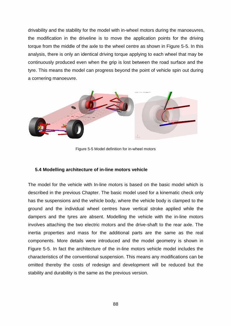
88

drivability and the stability for the model with in-wheel motors during the manoeuvres,

the modification in the driveline is to move the application points for the driving

torque from the middle of the axle to the wheel centre as shown in Figure 5-5. In this

analysis, there is only an identical driving torque applying to each wheel that may be

continuously produced even when the grip is lost between the road surface and the

tyre. This means the model can progress beyond the point of vehicle spin out during

a cornering manoeuvre.

Figure 5-5 Model definition for in-wheel motors

5.4 Modelling architecture of in-line motors vehicle

The model for the vehicle with In-line motors is based on the basic model which is

described in the previous Chapter. The basic model used for a kinematic check only

has the suspensions and the vehicle body, where the vehicle body is clamped to the

ground and the individual wheel centres have vertical stroke applied while the

dampers and the tyres are absent. Modelling the vehicle with the in-line motors

involves attaching the two electric motors and the drive-shaft to the rear axle. The

inertia properties and mass for the additional parts are the same as the real

components. More details were introduced and the model geometry is shown in

Figure 5-5. In fact the architecture of the in-line motors vehicle model includes the

characteristics of the conventional suspension. This means any modifications can be

omitted thereby the costs of redesign and development will be reduced but the

stability and durability is the same as the previous version.

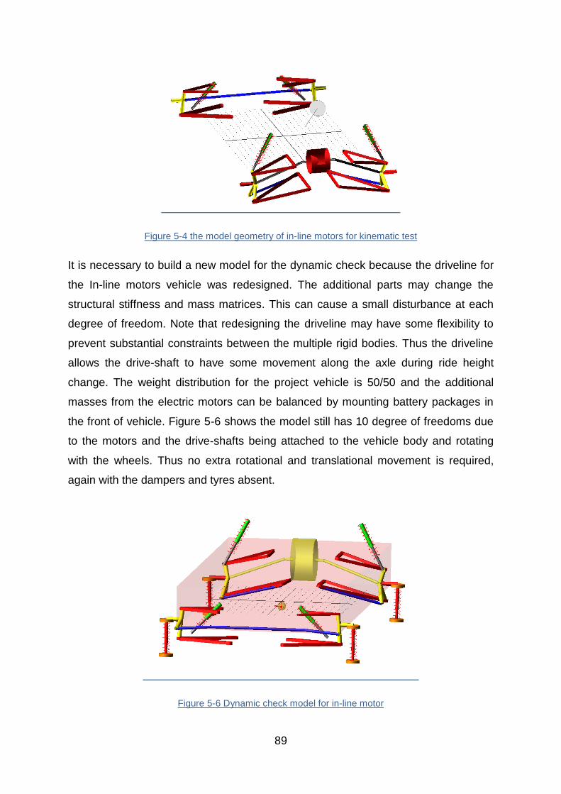
89

Figure 5-4 the model geometry of in-line motors for kinematic test

It is necessary to build a new model for the dynamic check because the driveline for

the In-line motors vehicle was redesigned. The additional parts may change the

structural stiffness and mass matrices. This can cause a small disturbance at each

degree of freedom. Note that redesigning the driveline may have some flexibility to

prevent substantial constraints between the multiple rigid bodies. Thus the driveline

allows the drive-shaft to have some movement along the axle during ride height

change. The weight distribution for the project vehicle is 50/50 and the additional

masses from the electric motors can be balanced by mounting battery packages in

the front of vehicle. Figure 5-6 shows the model still has 10 degree of freedoms due

to the motors and the drive-shafts being attached to the vehicle body and rotating

with the wheels. Thus no extra rotational and translational movement is required,

again with the dampers and tyres absent.

Figure 5-6 Dynamic check model for in-line motor

90

Figure 5-7 shows a completed model for a drivability check in which the dampers

and tyres are now present. According to the configuration for the In-line motors

vehicle model, the points for applying the driving torque move to the position where

the motor and the drive shaft connect together. These retrofits to the architecture are

intended to improve vehicle drive efficiency in which the new driveline has less

mechanical components and a direct drive design. The efficiency of a conventional

driveline is about 20% and an electric vehicle with in-wheel motors increases to

approximately 80% depending on the driving cycle. However, the common

architecture for in-wheel motors vehicles includes a shorter driveline than in-line

motors vehicles, but requires major modifications to traditional suspensions to

include the power source.

Figure 5-7 A full vehicle model for drivability check

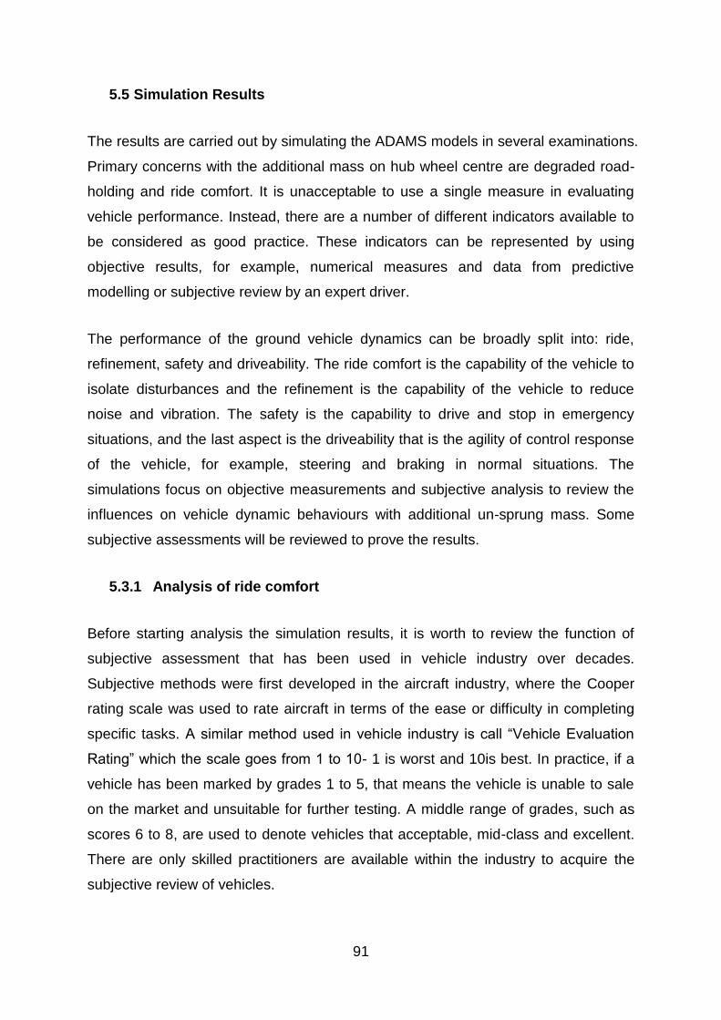
91

5.5 Simulation Results

The results are carried out by simulating the ADAMS models in several examinations.

Primary concerns with the additional mass on hub wheel centre are degraded road-

holding and ride comfort. It is unacceptable to use a single measure in evaluating

vehicle performance. Instead, there are a number of different indicators available to

be considered as good practice. These indicators can be represented by using

objective results, for example, numerical measures and data from predictive

modelling or subjective review by an expert driver.

The performance of the ground vehicle dynamics can be broadly split into: ride,

refinement, safety and driveability. The ride comfort is the capability of the vehicle to

isolate disturbances and the refinement is the capability of the vehicle to reduce

noise and vibration. The safety is the capability to drive and stop in emergency

situations, and the last aspect is the driveability that is the agility of control response

of the vehicle, for example, steering and braking in normal situations. The

simulations focus on objective measurements and subjective analysis to review the

influences on vehicle dynamic behaviours with additional un-sprung mass. Some

subjective assessments will be reviewed to prove the results.

5.3.1 Analysis of ride comfort

Before starting analysis the simulation results, it is worth to review the function of

subjective assessment that has been used in vehicle industry over decades.

Subjective methods were first developed in the aircraft industry, where the Cooper

rating scale was used to rate aircraft in terms of the ease or difficulty in completing

specific tasks. A similar method used in vehicle industry is call ―Vehicle Evaluation

Rating‖ which the scale goes from 1 to 10- 1 is worst and 10is best. In practice, if a

vehicle has been marked by grades 1 to 5, that means the vehicle is unable to sale

on the market and unsuitable for further testing. A middle range of grades, such as

scores 6 to 8, are used to denote vehicles that acceptable, mid-class and excellent.

There are only skilled practitioners are available within the industry to acquire the

subjective review of vehicles.

92

According to Anderson and Harty (2010) have tested a 2007 Model Year Ford Focus

that was added 30kg additional mass to each wheel centre. This approach assumes

rotating and non-rotating un-sprung masses in a way which broadly reflects the in-

wheel motors. No other changes were made to the vehicle, which is to say no

development was performed for the purpose of this exercise.

Subjective – Figure 5-8 shows the subjective result plot for ride evaluation. Some

degradation can be found in the pitch control, small impact feel and large impact feel.

Nothing in need of attention in the roll movement is described by the skilled

practitioner.

Figure 5-8 Subjective results for ride testing (Anderson and Harty 2010)

Objective – As well as the subjective reviews carried out, objective measurements

are made of ride comfort by using the in-line and in-wheel motors models that were

built in previous section. The vehicle body is free and the platforms under wheels

impart surface motion into the suspensions. The tyres represented by single spring

damper and can separate from platforms under large inputs. The simulation runs at

the dynamic mode for two second and to examine the vehicle models for their

eigenvalues – Natural Frequencies at each degree of freedoms. The results show in

Table 5-1. The information includes: sequential number of the mode that was

predicted by the Eigen solution, natural frequency corresponding to the mode,

damping ratio for the mode and list the real and imaginary part of the eigenvalue.

This item has been removed due to third party copyright. The unabridged version of the thesis can be viewed at the Lanchester Library, Coventry University.

93

It is often true with passenger vehicles that the primary ride roll mode is at a higher

frequency than the other two primary ride modes, since the anti-roll (―stabilizer‖) bars

add a large amount of stiffness to the roll mode. Wheel hop frequencies are high

compared to passenger car values but again the racing nature of the vehicle means

the vertical tyre stiffness is relatively high, increasing up the wheel hop frequency.

The four wheel hop modes are sensibly positioned with respect to each other, with

the front modes, influenced by the steering gear mass.

Table 5-1 Display the eigenvalues in tabular form

Table 5-2 Explanation of natural frequencies at each mode

Mode Frequency Comment

1-3 <0.2Hz Body on rig stabilisation springs – fore-aft, yaw ,lateral

4 1.389 Hz Primary Ride 1 – Heave

5 2.465 Hz Primary Ride 2 – Pitch

6 3.487 Hz Primary Ride 3 – Roll

7 12.56 Hz Rear left wheel hop

8 12.68 Hz Rear right wheel hop

9 18.94 Hz Front left wheel hop

10 19.14 Hz Front right wheel hop

94

The calculation for eigenvalues and eigenvectors can be performed using a function

of ADAMS which provides a prediction of the model‘s natural frequencies and mode

shapes. After the calculation is complete, ADAMS can display the Eigenvalues in

tabular form and also plot complex Eigenvalues scatter as shown in Figure 5-9.

Finding the stability of the system depends on the real and imaginary parts of the

Eigenvalues, along with the positive or negative signs of the real parts and the

difference of their values.

The system is unstable when the sign of the real part is positive, and its behaviour is

more like an unstable oscillator. Comparatively, the system is stable when the real

part is negative. To consider a more complex system, it is important to note that the

system should has all real parts of the Eigenvalues with the negative values, and it is

necessary condition to determine the system is stable. In additional, when the

system is stable, the Eigenvalues should have the imaginary parts and that are not

equal to zero. However, the model is a stable system in which the all real values are

negative and the system has imaginary part that a pair of the values corresponds to

the each mode.

Figure 5-9 Eigenvalues for in wheel motors model

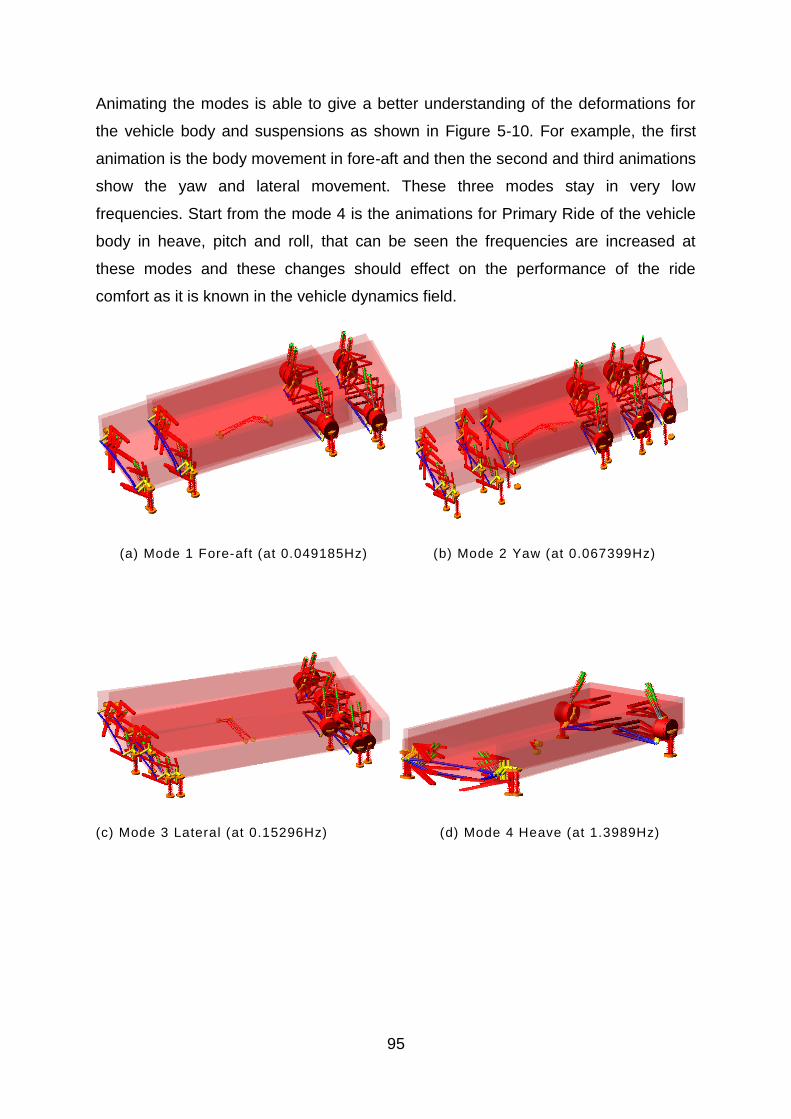
95

Animating the modes is able to give a better understanding of the deformations for

the vehicle body and suspensions as shown in Figure 5-10. For example, the first

animation is the body movement in fore-aft and then the second and third animations

show the yaw and lateral movement. These three modes stay in very low

frequencies. Start from the mode 4 is the animations for Primary Ride of the vehicle

body in heave, pitch and roll, that can be seen the frequencies are increased at

these modes and these changes should effect on the performance of the ride

comfort as it is known in the vehicle dynamics field.

(a) Mode 1 Fore-aft (at 0.049185Hz) (b) Mode 2 Yaw (at 0.067399Hz)

(c) Mode 3 Lateral (at 0.15296Hz) (d) Mode 4 Heave (at 1.3989Hz)

96

(e) Mode 5 Pitch (at 2.46543Hz) (f ) Mode 6 Roll (at 3.48793Hz)

Figure 5-10 The animations for vehicle body

It is often true with racing vehicles that the roll mode of primary ride is at a higher

frequency than other two primary ride modes, since the anti-roll bars add a large

amount of stiffness to the roll mode. In addition, the vehicle body as modelled is built

by using a single rigid body that may give large torsion stiffness for the vehicle

structure in roll mode. As well as known, the stiffness of body structure is another

open task to improve the vehicle handling and drive performance, likewise effects on

safety requirements as a major issue in vehicle industry. Figure 5-11 shows the

animations in wheel hop modes at front and rear suspensions.

(a)Mode 7 Left wheel hop (at 12.563Hz) (b) Mode 8 Right wheel hop (at 12.681Hz)

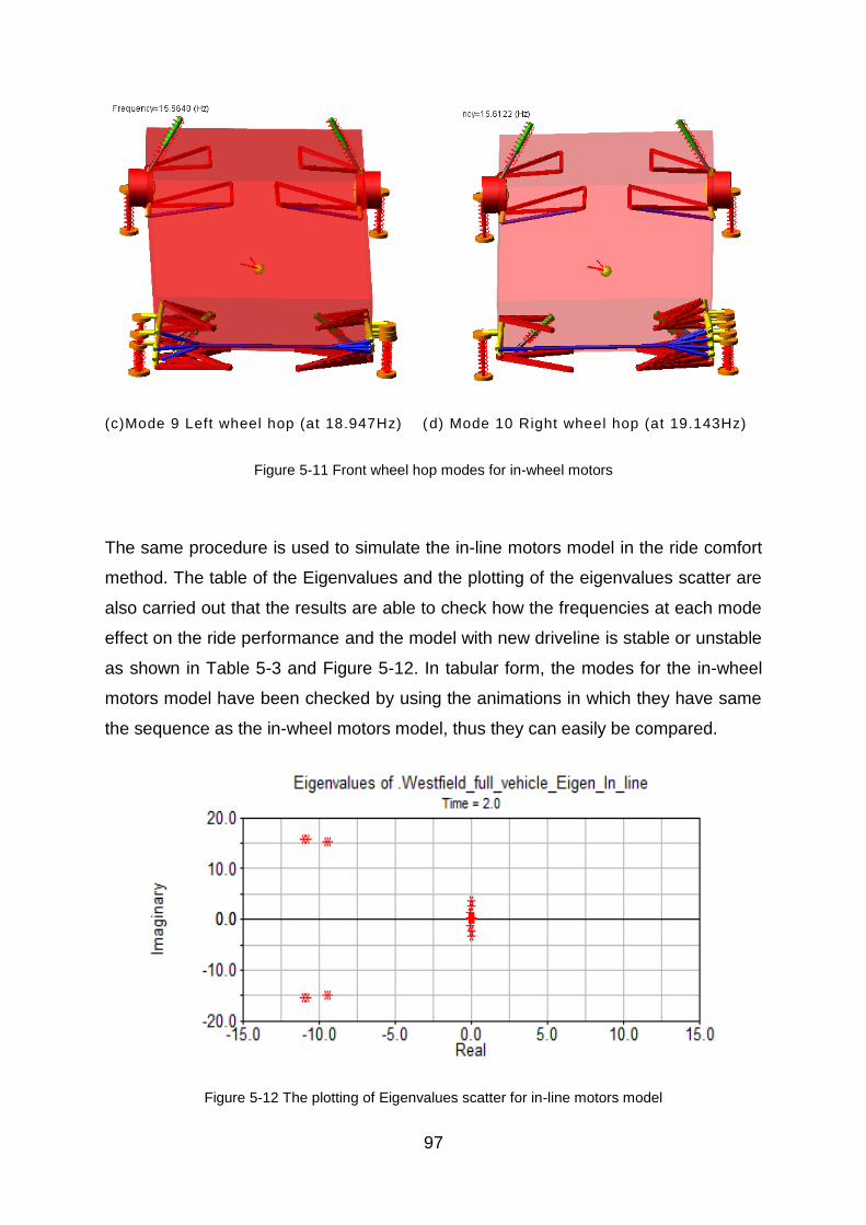
97

(c)Mode 9 Left wheel hop (at 18.947Hz) (d) Mode 10 Right wheel hop (at 19.143Hz)

Figure 5-11 Front wheel hop modes for in-wheel motors

The same procedure is used to simulate the in-line motors model in the ride comfort

method. The table of the Eigenvalues and the plotting of the eigenvalues scatter are

also carried out that the results are able to check how the frequencies at each mode

effect on the ride performance and the model with new driveline is stable or unstable

as shown in Table 5-3 and Figure 5-12. In tabular form, the modes for the in-wheel

motors model have been checked by using the animations in which they have same

the sequence as the in-wheel motors model, thus they can easily be compared.

Figure 5-12 The plotting of Eigenvalues scatter for in-line motors model

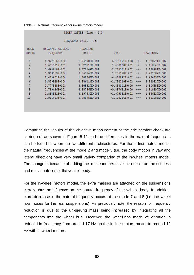
98

Table 5-3 Natural Frequencies for in-line motors model

Comparing the results of the objective measurement at the ride comfort check are

carried out as shown in Figure 5-11 and the differences in the natural frequencies

can be found between the two different architectures. For the in-line motors model,

the natural frequencies at the mode 2 and mode 3 (i.e. the body motion in yaw and

lateral direction) have very small variety comparing to the in-wheel motors model.

The change is because of adding the in-line motors driveline effects on the stiffness

and mass matrices of the vehicle body.

For the in-wheel motors model, the extra masses are attached on the suspensions

merely, thus no influence on the natural frequency of the vehicle body. In addition,

more decrease in the natural frequency occurs at the mode 7 and 8 (i.e. the wheel

hop modes for the rear suspensions). As previously note, the reason for frequency

reduction is due to the un-sprung mass being increased by integrating all the

components into the wheel hub. However, the wheel-hop mode of vibration is

reduced in frequency from around 17 Hz on the in-line motors model to around 12

Hz with in-wheel motors.

99

It is clear shown in Figure 5-11 (a), which the frequencies at the rear wheel hop

modes are obviously different, and that should change the level of response, but not

significant. There are no testing results to indicate that the vibrations of unsprung

mass from 12 to 17Hz will produce more noisome, thus it may be summarized that

the ride behaviour is not substantially changed by adding the masses on the wheel

centre.

Table 5-4 Comparison of natural frequencies for in-line and in-wheel motors model

(a) In-wheel motors (b) In -line motors

Nevertheless it is necessary to introduce another simulation for further ride comfort

check in which an inspection in the vertical wheel hub acceleration will be needed to

verify any influences of ride behaviour due to the additional masses. A typical

method has developed by Blundell (2004) who defined a motion imparted to a jack

part to represent inputs from the road surface, and a step function can also be used

to describe a profile of speed bump as shown in Figure 5-13. Motion in translational

applies on the jack to give the suspension an severe impact, and the result shows in

Figure 5-14 over a large single disturbance the in-wheel motors model gives

measurably poorer behaviour – higher and severe response, that can elucidate why

the in-wheel motors vehicle provides lower score on subjective assessment.

100

Figure 5-5 Road profile for speed bump (Blundell, 2004)

Figure 5-6 Measured results for wheel hub acceleration

5.3.2 Analysis of drivability check

As mentioned, it is very important to work out how the additional masses will effect

on the drive safety and control performance of electric vehicles with different

architectures. Reasonably, some reviews in subjective evaluations of real vehicle

testing environment will be carried out as following, and therefore the driver

sensitivity at the level of expert can define the response of the vehicle precisely and

101

give an authentic score in vehicle evaluation rating. The previous comparisons

mainly focus on the ride comfort check with extra masses on the rear wheels, and

that are very useful evidences to elucidate the advantages of architecture for in-line

motors vehicle. More objective measurements in drivability will be accomplished still

with more interested results.

Subjective – The subjective result of drivability check is shown in Figure 5-15, and

the largest deficit concern is the effort in the steering in which becomes heavier

under a large range of circumstances. The degradations obviously effect on the

drivability of the in-wheel motors vehicle at obstacle avoidance and emergency turns,

even need more efforts on parking. Nevertheless, the architecture for in-line motors

vehicle has a typical or traditional chassis in which the drivability can be expected as

same as a performed vehicle.

Figure 5-15 Subjective results of steering behaviour (Anderson and Hart, 2010)

Objective – The previous models for the drivability check are taken into the

computer-based (ADAMS) simulation. The simulation consists of two manoeuvres:

steady state cornering and double lane change. For first step, the analysis for steady

state cornering is carried on a 40m radius course, and a closed-loop driver model

uses PID controller in which strong emphasis on Integral gain gives the model

accurate path following. The simulation starts with a speed of around 5kmh and the

This item has been removed due to third party copyright. The unabridged version of the thesis can be viewed at the Lanchester Library, Coventry University.

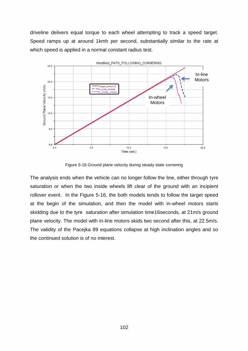
102

driveline delivers equal torque to each wheel attempting to track a speed target.

Speed ramps up at around 1kmh per second, substantially similar to the rate at

which speed is applied in a normal constant radius test.

Figure 5-16 Ground plane velocity during steady state cornering

The analysis ends when the vehicle can no longer follow the line, either through tyre

saturation or when the two inside wheels lift clear of the ground with an incipient

rollover event. In the Figure 5-16, the both models tends to follow the target speed

at the begin of the simulation, and then the model with in-wheel motors starts

skidding due to the tyre saturation after simulation time16seconds, at 21m/s ground

plane velocity. The model with in-line motors skids two second after this, at 22.5m/s.

The validity of the Pacejka 89 equations collapse at high inclination angles and so

the continued solution is of no interest.

In-line Motors

In-wheel Motors

103

Figure 5-17 The trajectories at cornering

More effects can be seen in the trajectories at steady state cornering as shown in

Figure 5-17. In side pushing effect of vehicle scenario, the model with in-wheel

motors reaches the performance limits quicker and exhibits more understeer

behaviour. The model with in-line motors induces extra yaw moment, helping the

vehicle reduces understeer behaviour, thereby reducing the steering angle required.

Figure 5-18 clearly shows that the centripetal acceleration is less with in-line motors.

104

Figure 5-7 Testing results for centripetal acceleration of in-line and in-wheel motors

In the next step, the models will be taken into double lane change manoeuvre. The

manoeuvre is essential a scaled version of ISO3888 lane change in its geometry,

only the test protocol differs slightly. It consists of a defined zone in which the vehicle

can take any path and reflects a real world avoidance manoeuvre within a finite width

road. The vehicle must displace laterally by around 3.5m minimum and then return to

its original path. The modification of the double lane change is intended to reflect

maximum effort manoeuvring at highway speeds and the length and width of the

manoeuvring zone are related to the vehicle proportions, as shown in Figure 5-19.

Also the details for optimizations of double lane change will be discussed in the next

Chapter.

In-line Motors

In-wheel Motors

105

Figure 5-8 Double Lane Change Test Course

With real vehicle, the driver skill levels modify the performance of a given vehicle

through the lane change substantially and so when comparing vehicles it is

preferable to use a panel of drivers or at least a consistent driver. In the analysis the

driver model is consistent and repeatable as well the closed-loop PID control gives

the vehicle an accurate path following.

For the simulation, the both models are driven up to the manoeuvre start at 100km/h

and the throttle released. The overrun condition is typically the most difficult in terms

of stability. Although the vehicle loses speed as it enters the second of the two

manoeuvres, it is typically unsettled dynamically and so the second transition is often

the more problematic of the two. The maximum variation of yaw rate can be seen in

the stage of centre correction and exit oscillations, there is that the increased angular

velocity in yaw around 8 degree/s emerges an overshot at the peak values

comparing to in-line motors model as shown in Figure 5-20. Also some influences of

body slip angle are shown in Figure 5-21, which is important because it effectively

grows the width of the vehicle. The changes are large enough to indicate the driver

the vehicle will be lost control. The measurements based on computing simulations

are broadly familiar with subjective assessments, which more evidences will be

shown in next section to see somewhat worse results as expected.

106

Figure 5-9 Comparison of yaw rate for in-line and in-wheel motors in DLC

Figure 5-10 Comparison body slip angle for in-line and in-wheel motors in DLC

Considering driver steering motion inputs for both models, it can be seen in Figure 5-

22, the model with the in-line motors has a large reduction about 10 degrees in first

reversal and centre correction section, also a useful improvement in overall

magnitude of steering angle inputs can be found. In addition, there is an improved

quality to the steering traces in terms of smoothness and lack of reversals when the

model with in-line motors. It may expect more significant differences in driveability

Centre correction

Exit oscillations

107

check when comparing the two architectures, nevertheless considering the change

on in-wheel motor model is only to add 5% of the entire vehicle weight into the rear

wheel centre and the extra weight is even less than a passenger.

Figure 5-11 Comparison of steering angle for in-line and in-wheel motors in DLC

5.5 Conclusion

In this chapter, the vehicle architectures of in-wheel motor and in-line motor are

introduced that the significant modifications of original suspension have been done

to integrate all components of in-wheel motors, such as braking system, cooling

system and electric motors, into the constraint volume at inside of the rim.

Furthermore, the un-sprung mass is obvious increased for implementing in-wheel

motors on a vehicle, and degraded ride and handling performance. Compare to the

architecture of in-wheel motors vehicle, the in-line motors vehicle were required the

minimum variations of suspension system thus is can remain the un-sprung masses

and reduce redesign costs.

Objective measurements were carried out by using several computing simulation

models in ADAMS, such as kinematic, dynamic and handling models. The aspects of

simulation have been examined in detail and can be concluded thus the overall

performance of ride comfort is demoted and the obvious impact of steering

First turn in

First reversal

Centre correction

Exit oscillations

108

behaviour emerge with testing the vehicle models in cornering and lane change

manoeuvres. The effects on safety and driveability are required some variations in

suspension component detail and increase in damping levels to restore agility.

Overall, developing the electric vehicle in next recent state the architecture of in-line

motors vehicle can preserve the characteristics of conventional vehicle in high

performance, and the redesign costs and efforts can be economized on improving

capacity of electric motors and battery life. Moreover the good potential of individual

wheel motor control can be implemented by using in-line wheel motors for

substantial improvements in vehicle behaviour.

109

6 Torque vectoring system with in-line motors

6.1 Introduction

Active intelligent control systems for achieving vehicle stability and handling have

been developed and implemented to enhance the driving safety and performance of

the driving vehicle. Some enhancements, such as Active Steering Systems and

Electronic Stability Programs, can help the driver to retain control of their vehicles

when the grip between road surface and tyre is lost. In previous investigations, the

ABS based Stability Control Systems are principal safety implement to accomplish

the safety requirements under adverse road conditions. However, the vehicle speed

is degraded while the Stability Control System implements braking force on four

wheels individually to improve the correct position of the vehicle body. Moreover, the

Torque Vectoring (TV) system can be designed to improve the vehicle handling

qualities and avoid the vehicle speed decrease, or in other words the ‗fun-to-drive‘

aspect. Thus, torque vectoring can be used to influence the driver experience.

In this chapter, the investigation focuses on developing and designing a novel TV

control strategy that is called Optimal Driveline Control Strategy (ODCS). The ODCS

involves three levels of control: Desired Dynamics Behaviours, Secondary Control

and Advanced Torque Vectoring Control, more details of which will be represented in

the following section. Reviewing the basic principles for TV control on the

conventional driveline helps to understand how to implement those control strategies

on the pure electric vehicle. The configuration of the ODCS algorithm is clearly

shown in this chapter, and each level of control is explained in detail.

The project vehicle model with three different types of drivelines is taken into

Computer-Based simulations. The results are carried out by running the vehicle

model through the steady state cornering and lane change manoeuvres. The results

for the vehicle model with ODCS are also compared against the conventional

drivelines, such as Open and Limited Slip Differential, during which the vehicle

speed is increased.

110

6.2 Basic principles

The conventional drivelines, such as Open Differential and Limited-Slip Differential,

have been broadly used in the rear driving vehicles. The Open Differential allows the

driving wheels to rotate at different speeds while giving the same driving torques on

both wheels. The Limited-Slip Differential is designed to improve handling and

stability while the vehicle turns into a corner, but a fixed kinematic relationship can

only transfer the driving torques from the faster spinning wheel to the slower wheel

(Mohan and Sharma, 2006). Thus, developing a Torque Vectoring system is required:

first to retain the abilities of the open differential and limited slip differential, and then

to incorporate a means to vary the kinematic ratio across the differential thus

affecting the torque distribution between the wheels.

Figure 6-1 Definition of torque vectoring differential

⁄ ⁄ (6.2.1)

⁄ ⁄ (6.2.2)

⁄ (6.2.3)

⁄ (6.2.4)

111

Figure 6-1 shows a basic principle of TV applied to the rear axle when turning the

vehicle left, the engaging clutches can transmit the engine torque via the pro-shaft

from left driving wheel to right side with transferring torque . In addition, adding or

subtracting the driving torques on the left and the right wheels give a difference

on the longitudinal driving force. The difference generates additional yaw moment

to help the vehicle turn into the corner more easily.

Here is a good example in Figure 6.2.2 to show how to accomplish the requirements

of TV by using a mechanism TV differential. The system includes planetary gears

and slipping multi-plate wet clutches, which those components are controlled by

electromechanical or electrohydraulic control systems (Li and Wu, 2011). In addition,

the functions of TV system can be applied to all types of driving vehicles, such as

Rear-Wheel-Drive (RWD), Front-Wheel-Drive (FWD), and Four-Wheel-Drive (4WD),

which the device enables to be mounted on either front, rear or both axles to modify

engine torque to each wheel. Closed-Loop Control is used in the system, thus the

vehicle speed, wheel slip ratio, yaw rate error and other parameters have to be

measured. The outputs from the measurements are used to modify the driving

torques from an Internal Combustion engine.

Figure 6-2 Schematic of a mechanism torque-vectoring differential

(Mohan and Sharma, 2006)

This item has been removed due to third party copyright. The unabridged version of the thesis can be viewed at the Lanchester Library, Coventry University.

112

Reviewing the schematic of a mechanism TV differential in Figure 6-2, the device

uses stepped planets and sun gears meshing each other to provide for a differential

action. The biasing gear-set is connected to the wet clutch as brakes that can slow

down one side and speed up on the other side thereby allowing the driven vehicle to

be turned. The secondary gears enable the reduction of the brake torque required to

steer the vehicle, and thus increase the efficiency of the system.

Figure 6-3 Explanations of the left-and-right torque vectoring

In order to explain how the functions of a TV system can be implemented on the

project vehicle clearly, a schematic that shows the relationship between driving

forces and maximum cornering forces is carried out in Figure 6-3. The project vehicle

is pure electric vehicle with the Rear-Wheel-Drive, thus a mechanism driveline is

replaced by a pair of electric motors at the middle of the rear axle where a differential

is located. Moreover, the characteristics defined in the previous chapter indicate the

project vehicle is under-steer and the weight distribution is 50/50 so the maximum

friction circles are symmetric at the front and rear wheels when driving the vehicle in

a straight line. According to the configurations of the project vehicle, only a Left-and-

Right TV control has been considered in this research. The schematic shows that

assuming the vehicle model is turning left, lateral acceleration causes the right wheel

maximum friction circle to increase and the left wheel maximum friction circle to

113

decrease. If using a function of Open Differential on project vehicle, for example, the

driving torques are identical at two rear wheels and only the right tyre generates

cornering force because the maximum tyre friction force is bigger than the

driving force. However, using a Left-and-Right TV configuration is possible to

redistribute the engine torque between the two wheels, thus the left driving force will

be and the right driving force is , so that both the driving wheels

generate the maximum cornering forces compared to the vehicle without TV control.

The additional cornering force can be expressed as below:

(6.2.5)

So √

(

)

√

(

)

(

) (6.2.6)

Based on this formula, when the vectoring torque is applied, the additional

cornering force will become a maximum value as shown below. It shows that the

vectoring torque generates the additional cornering force.

⁄ (6.2.7)

In order to implement this concept into the handling and stability control of the project

vehicle, a control strategy will be designed in the next section. Moreover, the

promise of individual motor control shows good potential for substantial

improvements in vehicle behaviour. It is worth mentioning, a mechanism TV

differential is difficult to apply the vectoring torques to the driving wheels when the

vehicle is on ―throttle off‖ position. A solution has been found by adding electric

equipment to the driving axle, thus enabling the extra propulsion forces to be

𝐹𝑙𝑚𝑐 𝑎𝑛𝑑 𝐹𝑟𝑚𝑐

: Left and right maximum cornering force with TV

𝐹𝑟𝑚𝑐: Right maximum cornering force without TV

𝐹𝑙𝑚𝑓⬚ 𝑎𝑛𝑑 𝐹𝑟𝑚𝑓

⬚ : Left and right maximum tyre friction force

𝐹𝑑: Driving force

𝐹𝑐

114

obtained. However, those issues will also be taken into account for creating a novel

control strategy.

6.3 Optimal Driveline Control Strategy (ODCS)

An Optimal Driveline Control Strategy (ODCS) is designed and developed in this

section. The aims of the control are to improve the project vehicle handling and

lateral stability; thus, to achieve those requirements the design concepts will be

based on the Left-and-Right TV control configuration and have three levels of control.

The outputs from the control strategy can dominate the pair of electric motors

individually.

A detailed diagram of the Optimal Driveline Control Strategy is exhibited in Figure 6-

4, which consists of three levels: Desired Dynamics Behaviours, Secondary Control

and Advanced Torque-Vectoring Control. The first level is created to define the

operating scope and desired behaviours. The desired behaviours are able to be

found according to the vehicle speed and path curvature calculation. The secondary

control is created to implement the desired driving torques and yaw rate error

correction for tracking the desired behaviours. The inputs from the upper levels

should dominate the electric motors through the Advanced Torque Vectoring Control

(ATVC). The use of ATVC level is to modify the vectoring torques and driving

torques outputs, and some constraints are added to avoid wheel slip while

accelerating or braking.

115

Figure 6-4 Schematic of Driveline Control Strategy (DCS)

In addition, a human driver model is required to simulate the project vehicle. The

performance of a real vehicle, through road testing, can be modified by driver skill

levels; so it is preferable to use a consistent driver when comparing the vehicles.

Moreover, the aim of the DCS is to assist the driver to cope with the extreme driving

scenarios even in the ―throttle off‖ condition. However, an Open-Loop Driver model is

used with the project vehicle to follow a desired path with consistent driving

116

performance. Thus the simulated results from the model with different driving

configurations and vehicle speeds can be compared.

6.3.1 Definitions of Desired Dynamics Behaviour

Reference model definition

The primary requirement of the ODCS is to deliver desired dynamics behaviour in

terms of the desired path, desired yaw rate, operating scope and vehicle linearity.

The vehicle as modelled in the previous chapter will be taken into a steady state

cornering manoeuvre for the first simulation. The yaw rate transfer function of the

vehicle without TV control (the so-called ―baseline vehicle‖) can be obtained from the

equations describing the lateral force and yaw dynamics of the single-track vehicle

model (Milliken, 1995). Thus

(6.2.8)

In this equation, is the mean steer angle of the front wheels. The stability

derivatives can be expressed as a function of the front and rear cornering stiffnesses,

i.e. and , respectively, as

These equations are correctly referred to as a 2-degree-of-freedom model; they are

sometimes referred to as a ‗bicycle‘ model but this description should not imply that

the description may be suitable for two-wheeled vehicles.

The next hurdle to be crossed is the representation of the intended behaviour of the

vehicle – the ‗reference‘ states. Competition-developed lap simulation tools use a

‗track map‘ based on distance travelled and path curvature. This representation

allows the reference path to be of any form at all and allows for circular or crossing

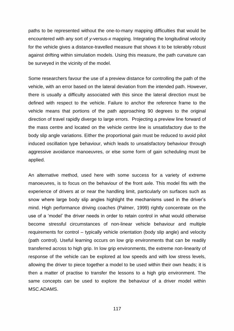
117

paths to be represented without the one-to-many mapping difficulties that would be

encountered with any sort of y-versus-x mapping. Integrating the longitudinal velocity

for the vehicle gives a distance-travelled measure that shows it to be tolerably robust

against drifting within simulation models. Using this measure, the path curvature can

be surveyed in the vicinity of the model.

Some researchers favour the use of a preview distance for controlling the path of the

vehicle, with an error based on the lateral deviation from the intended path. However,

there is usually a difficulty associated with this since the lateral direction must be

defined with respect to the vehicle. Failure to anchor the reference frame to the

vehicle means that portions of the path approaching 90 degrees to the original

direction of travel rapidly diverge to large errors. Projecting a preview line forward of

the mass centre and located on the vehicle centre line is unsatisfactory due to the

body slip angle variations. Either the proportional gain must be reduced to avoid pilot

induced oscillation type behaviour, which leads to unsatisfactory behaviour through

aggressive avoidance manoeuvres, or else some form of gain scheduling must be

applied.

An alternative method, used here with some success for a variety of extreme

manoeuvres, is to focus on the behaviour of the front axle. This model fits with the

experience of drivers at or near the handling limit, particularly on surfaces such as

snow where large body slip angles highlight the mechanisms used in the driver‘s

mind. High performance driving coaches (Palmer, 1999) rightly concentrate on the

use of a ‗model‘ the driver needs in order to retain control in what would otherwise

become stressful circumstances of non-linear vehicle behaviour and multiple

requirements for control – typically vehicle orientation (body slip angle) and velocity

(path control). Useful learning occurs on low grip environments that can be readily

transferred across to high grip. In low grip environments, the extreme non-linearity of

response of the vehicle can be explored at low speeds and with low stress levels,

allowing the driver to piece together a model to be used within their own heads; it is

then a matter of practise to transfer the lessons to a high grip environment. The

same concepts can be used to explore the behaviour of a driver model within

MSC.ADAMS.

118

Desired Yaw Rate

This section describes the methodology for the definition of desired yaw rate for the

controller implemented on the vehicle model with nonlinear dynamics. A target

under-steer characteristic is defined in terms of an analytical function relating the

dynamic steering-wheel angle (where is the actual steering-wheel

angle, and is the kinematic steering-wheel angle) to the lateral acceleration .

Therefore, Shibahata (1993) proposed a method based on the following three

characteristic parameters: the under-steer gradient ; the threshold

value , which defines the upper limit of the linear part of the under-steer

characteristic; and the maximum lateral acceleration achievable in trimmed

conditions . Thus

( )

( )

Where ), and

. The terms , , and

can be chosen according to the control design requirements. In particular, the same

value of at different values of the longitudinal acceleration have been considered,

to achieve the compensation of the variation of the under-steer gradient in traction

and braking conditions. Following Shibahata (1993), the steady-state value of the

desired yaw rate is given by

⁄

All equations allow the generation of the desired yaw rate as a function of vehicle

speed, steering-wheel angle, longitudinal acceleration, and friction coefficient at the

tyre-road contact. At the starting point, finding a desired path for testing the vehicle

model under dynamics manoeuvres, i.e. steady state cornering and double lane

change, is important and it can be defined by using path curvature . The analysis

starts when the vehicle runs on a 33m diameter circle, and then a desired yaw rate

can be calculated by using the expression above.

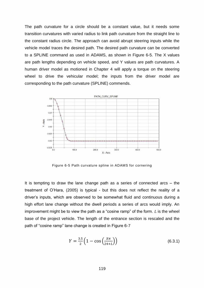
119

The path curvature for a circle should be a constant value, but it needs some

transition curvatures with varied radius to link path curvature from the straight line to

the constant radius circle. The approach can avoid abrupt steering inputs while the

vehicle model traces the desired path. The desired path curvature can be converted

to a SPLINE command as used in ADAMS, as shown in Figure 6-5. The X values

are path lengths depending on vehicle speed, and Y values are path curvatures. A

human driver model as motioned in Chapter 4 will apply a torque on the steering

wheel to drive the vehicular model; the inputs from the driver model are

corresponding to the path curvature (SPLINE) commends.

Figure 6-5 Path curvature spline in ADAMS for cornering

It is tempting to draw the lane change path as a series of connected arcs – the

treatment of O‘Hara, (2005) is typical - but this does not reflect the reality of a

driver‘s inputs, which are observed to be somewhat fluid and continuous during a

high effort lane change without the dwell periods a series of arcs would imply. An

improvement might be to view the path as a ―cosine ramp‖ of the form. is the wheel

base of the project vehicle. The length of the entrance section is rescaled and the

path of ―cosine ramp‖ lane change is created in Figure 6-7

( (

)) (6.3.1)

120

-3.5

0

0 5 10 15 20 25 30

Distance Travelled (m)

Late

ral P

ath

(m

)

Figure 6-6 Cosine ramp lane change path visualisation

When considering the task in detail, it is noted that the mid-section is wider than the

vehicle. When the position of the vehicle is fractionally away from the very edge of

the entrance gate, it is necessary to tune the relative length of the turn-in and turn-

out sections and to run out to the very widest part of the path available. Further slight

modification to the exact form is made to make it continuously differentiable as

shown in Figure 6-8. If this ―optimized cosine‖ form is compared with the initial cosine

form, a substantial reduction in centripetal acceleration is realised as shown in

Figure 6-9.

Figure 6-7 Optimized lane change path with the behaviours of real driver

-5

-4.5

-4

-3.5

-3

-2.5

-2

-1.5

-1

-0.5

0

0 5 10 15 20 25 30 35 40

Distance Travelled (m)

Insid

e W

he

el

La

te

ra

l P

ath

(m

)

Optimised Cosine

Cosine

NATO DCL Entrance

NATO DCL Mid Sect ion

NATO DCL Outer Limit for Inside Wheel

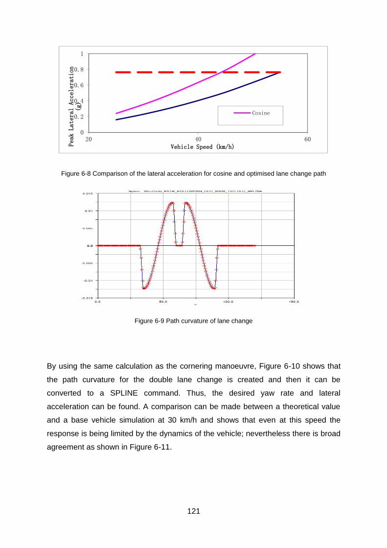
121

Figure 6-8 Comparison of the lateral acceleration for cosine and optimised lane change path

Figure 6-9 Path curvature of lane change

By using the same calculation as the cornering manoeuvre, Figure 6-10 shows that

the path curvature for the double lane change is created and then it can be

converted to a SPLINE command. Thus, the desired yaw rate and lateral

acceleration can be found. A comparison can be made between a theoretical value

and a base vehicle simulation at 30 km/h and shows that even at this speed the

response is being limited by the dynamics of the vehicle; nevertheless there is broad

agreement as shown in Figure 6-11.

0

0.2

0.4

0.6

0.8

1

20 40 60

Peak Lateral Acceleration

(g)

Vehicle Speed (km/h)

Cosine

122

Figure 6-10 Comparison of desired and actual lateral acceleration

An actual double lane change protocol calls for an increase in vehicle speed until the

driver is no longer able to complete the manoeuvre; the outcome from the test is the

highest speed at which the driver can repeatedly complete the manoeuvre. For this

simulation, the vehicle model runs from low speed 40 km/h to a high speed that is

close to the physical limitation of the vehicle model. Repeated iterations are made to

discover the optimal performance of the vehicle model that should be improved by

Driveline Control Strategy. Nevertheless, the reported vehicle behaviour is to

complete the manoeuvre at 110 km/h so that the lateral acceleration starts to exceed

the control region of the TV system. The ODCS is no longer to fulfil the safety

requirements, therefore the manoeuvre approaches an emergency stage requiring

the vehicle to reduce the speed to control its motion and diminish the kinetic energy

of the vehicle body by normal use of the braking or stability control system.

-0.25

0

0.25

-20 0 20 40 60 80 100

Ay(g)

ADAMS Ay(g)

123

Figure 6-11 Yaw Rate Gain (YRG) for three different vehicles (Blundell and Harty, 2004)

Normally, the vehicles need to be designed to reduce the Yaw Rate Gain (YRG) at

high speed to ensure the drivers still control the vehicle when faced with emergency

evasive manoeuvres. For typical road vehicles, the characteristics of the vehicle are

performed to have further modifications to reduce the yaw rate gain even when the

tyres are not saturated. These modifications are very different between different

demands as shown in Figure 6-12, in which all three vehicles are under-steer in their

linear regions, but yet the racing vehicle tends to increase yaw rate gain at higher

speed thus improving dynamic control performance for expert drivers because it is

closer to neutral steer. Reviewing the YRG characteristics for the WRC 2003 car,

some linear YRG points are very close, and are even over the neutral steer line

when the vehicle speed is around 50km/h. Moreover, the linear YRG points are

substantially decreased while the vehicle speed is over 100km/h.

Based on the YRG characteristics for racing vehicles, the TV control should

dominate the YRG of the project vehicle model close to their theoretical YRG curve.

Therefore, Figure 6-13 represents an operating region for the TV system in this

research. The theoretical YRG curve for the project vehicle was calculated in the

Chapter 4. Because of the characteristics being very close to the neutral steer when

the speed is below 80km/h, the use of TV control should maintain the model in its

own characteristics and prevent a bulk over-steer. The actual YRG may have a large

124

drop as shown while the vehicle speed is raised, thus The TV control is also required

to dominate the actual YRG approaching the theoretical curve.

Figure 6-12 Explanation of torque vectoring authority envelope

In Figure 6-13, the YRG for neutral steer and the theoretical YRG of the project

model can be calculated by using the equations below:

⁄

⁄ (6.3.5)

Note that the over-steer and under-steer can be easily known by a ratio of the

geometric yaw rate and wheel steer angle as shown in the equation 6.3.5. If the ratio

is more than 1, the vehicle is under-steer and if the ratio is less than 1, the vehicle is

over-steer.

Torque Vectoring

Authority

Neutral Steer

Theoretical YRG

𝑉: Vehicle speed

𝐿: Vehicle length

𝜔𝑔: Geometric yaw rate

𝛿

125

6.3.2 Secondary Control

The aim of secondary control design is to control the vehicle model tracking the

desired dynamics, which consists of the aspects of vehicle speed control, yaw rate

correction and control modes regulator. Rolling resistance and aerodynamic drag

forces are applied on this vehicle model, thus the vehicle speed is lost and also the

vehicle loses momentum during the resistant of the tyre cornering forces. Modelling

a speed compensation controller is required to offset the vehicle speed and the

inputs for the controller are dependent on the difference in the vehicle speed that is

measured between the ground plane velocity and the speed of the vehicle model.

Another controller for yaw rate correction is designed to minimise the difference

between the desired and the actual yaw rate. The outputs from this controller have a

substantial effect on the vectoring torques control. Finally, a regulator is added into

the Secondary Control to switch the Optimal Driveline Control Strategy (ODCS)

between the driving modes.

Speed Compensation (SC) Controller

In this simulation, a constant velocity of the vehicle needs to be maintained.

Therefore, a simple method of applying torque to the driven wheels is explained in

this section. The secondary control includes a Speed Compensation (SC) Controller

as part of the traction system, which means the torques are impart to the road

wheels and then produce tractive driving forces at the tyres. The ground plane

velocity as a reference speed can be calculated by using equation 6.3.6.

√

(6.3.6)

Hence, the tractive driving torques from the SC controller depend on the maximum

driving torques from the pair of electric motors, and the difference between the

ground plane velocity and longitudinal velocity of the vehicle model as shown

in equation 6.3.7

( | |) (6.3.7)

126

Based on ground reference frame, the direction of the velocity is negative so

using an absolute value for the velocity is necessary to ensure the driving torques

outputs in positive, which means the positive value gives the vehicle model a tractive

torque and the negative value may cause the vehicle to slow down. Note that the

maximum torque as output from the electric motors may produce large instant

tractive forces at the driven wheels when starting the simulation. It is necessary to

modify the torque to prevent the driving wheels slipping when the simulation

starts at different initial speeds. Therefore, an optimal output from the SC controller

will be taken into account in the third level of the ODCS.

Yaw Rate Error Correction (YREC)

The path curvatures for steady state cornering and lane change were detected in the

first level of the ODCS and hence the Desired Yaw Rate is found from the Path

Curvature and forward velocity using:

(6.3.8)

To apply the equation 6.3.8 to the simulation software, it needs to find out the path

length when the vehicle model runs at various speeds. Calculating the path length is

simply to integrate the ground plane velocity as shown below.

∫ ( )

6.3.9)

The body slip angle can be computed by using the equation 6.3.10 based on the

velocities of and .

(

) 3.10)

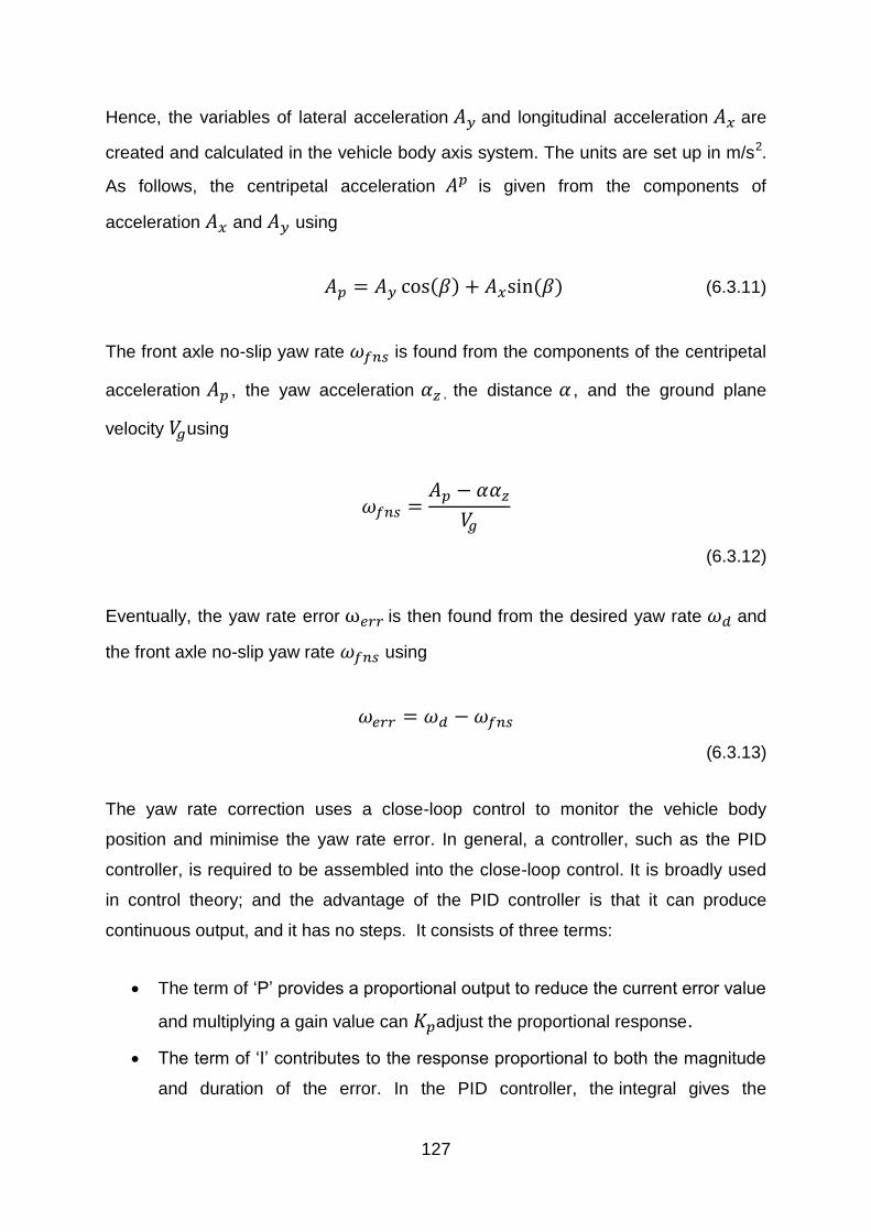
127

Hence, the variables of lateral acceleration and longitudinal acceleration are

created and calculated in the vehicle body axis system. The units are set up in m/s2.

As follows, the centripetal acceleration is given from the components of

acceleration and using

(6.3.11)

The front axle no-slip yaw rate is found from the components of the centripetal

acceleration , the yaw acceleration , the distance , and the ground plane

velocity using

(6.3.12)

Eventually, the yaw rate error is then found from the desired yaw rate and

the front axle no-slip yaw rate using

(6.3.13)

The yaw rate correction uses a close-loop control to monitor the vehicle body

position and minimise the yaw rate error. In general, a controller, such as the PID

controller, is required to be assembled into the close-loop control. It is broadly used

in control theory; and the advantage of the PID controller is that it can produce

continuous output, and it has no steps. It consists of three terms:

The term of ‗P‘ provides a proportional output to reduce the current error value

and multiplying a gain value can adjust the proportional response.

The term of ‗I‘ contributes to the response proportional to both the magnitude

and duration of the error. In the PID controller, the integral gives the

128

accumulated compensation from the previous correction and counts the total

of instantaneous error over time. Thus, the error can be minimized by

multiplying a gain value and that will be added to the controller output.

The derivative is the ‗D‘ item of the PID controller in which the derivative of the

error is calculated by determining the slope of the error over time, and the

derivative gain can adjust the rate of change.

In the ideal parallel form, the controller theory section for Yaw Rate Error Correction

(YREC) is shown below:

∫

(6.3.14)

Driving Modes Regulator

When simulating a vehicle model in manoeuvres, the use of several driving modes

enables determining the differences in vehicle dynamics handling and driving

performance. Therefore, the project vehicle is set up for three driving modes as

known: free rolling, driving with a differential, and TV control. The free rolling mode is

when the vehicle model is coasting through the manoeuvres without any propulsion

forces and only frictional force acts between road surface and tyre. The second

driving mode is to apply the use of an open differential to the model driveline to

produce an even torque at the driving wheels. The developed TV control is the third

driving mode in which the TV control should retain the function of the Open

Differential and Limited-Slip Differential, and it also has the ability to modify the

driving torque. Thus, a regulator has been designed to switch the SC controller and

YREC controller on/off between the driving modes automatically. In addition, when

the SC controller is off, the vehicle model does not have any propulsion forces at the

driving wheels. With this status, as mentioned, it is difficult for the mechanical

driveline to have the vectoring torque while retaining the position of the vehicle.

Nevertheless, the regulator can still force the ODCS to implement its function to

129

control the motors while the vehicle is turning; thus the vehicle enables having the

continuous vectoring torques at the driving wheels. To explain the use of the

regulator clearly, Table 6-1 shows how it switches between the driving modes.

Table 6-1 The schematic of control modes

Control Modes Driving Modes Speed Control Yaw Rate Error Correction

1 Coasting Deactivate Deactivate

2 Open Diff Activate Deactivate

3 Torque Vectoring Deactivate/Activate Activate

6.3.3 Advanced Torque Vectoring Control (ATVC)

In the previous section, the desired tractive driving forces from the speed

compensation and the desired yaw rate are determined. The inputs from the

secondary control level should be applied to the vehicle model through an Advanced

Torque Vectoring Control (ATVC) level. The ATVC is designed for the last level of

the ODCS and in order to modify the inputs from the previous control level. The aim

of this level should satisfy the conditions below.

Modifying the traction force for speed compensation

Optimizing the vectoring torque for yaw rate correction

Inspecting the driving efficiency

Modifying the traction force for speed compensation

In general, a speed compensation controller is derived to minimize the difference

between the ground plane speed and actual speed. The difference in the speed can

be modified by multiplying a constant gain . Normally the gain value is simply

set up for the maximum driving torque from the electronic motors; nevertheless, this

130

simplicity of the adjustment can cause some issues, such as longitudinal wheel slip,

when the vehicle runs at different speeds.

As a complex method, optimization can help and improve the overall design of the

product. If the process has a good design in early stage, the design cycle can be

shorted. In general, an optimization problem is described as a problem to minimize

or maximize an objective function over a selection of design variables, while

satisfying various constraints on the design and state variables of the system. The

objective function is normally represented by a numerical form of the quality, or

stability of the model. The aim for modifying the traction force for speed

compensation decides that the optimization chooses to find the maximum torque of

the traction as shown in Equation 6.3.15. The optimal value of this formula

corresponds to the best design possible that can give the optimal driving torques for

the speed compensation. Design variables can be thought of as the Ground Plane

Velocity for this design problem. The Ground Plane Velocity can be altered to define

the design results. In this study, the changes in the vehicle speed should result in

changes to the driving torque.

(

) | |

(6.3.15)

: Optimal torque for speed compensation

: Ground plane velocity

The difference in the vehicle speed can be minimized by multiplying an optimum gain

value as shown in Equation 6.3.16. Constraints are boundaries that directly or

indirectly eliminate unacceptable issues, thus a constraint for wheel slip is created to

keep the wheel slip ratio at driving wheels below a limit value . The constraint

only is applied when the actual wheel slip ratio is over the limitation; it also can

be explained by using the formula as below:

131

{

} | |

(6.3.16)

However, the ATVC is able to produce the optimized driving torque under the

constraint to compensate the speed. In this calculation, the design variable is set up

for the Ground Plane Velocity , thus the amplitude of the optimized torque

depends on two variables: the Ground Plane Velocity and the speed compensation.

Optimizing the vectoring torque for yaw rate error correction

A considerable change in yaw rate with vehicle speed can be perceived by the driver

as inconsistent vehicle behaviour during in normal driving conditions. To make the

vehicle behave more predictable, the TV control can be used (at least partially) to

compensate the variation of the yaw rate. However, the outputs from secondary

control are not precise enough and, thus, cannot provide a-priori definable amount of

vectoring torque.

The inputs from the yaw rate correction at the secondary control level should be

applied to the project model through the ATVC. As is known, the terms of the PID

controller can give a precise and rapid response in the yaw rate correction, but it is

still necessary to tune the gain values for the proportional, integral and derivative

terms. In general, the gain values are modified manually and are closely related to

the amplitude of the vectoring torque. Due to the variation in the vehicle speed, the

gain values over all the simulations are required in order to modify the amplitude

automatically. This means that the optimal vectoring torque inputs are able to adjust

the position of the vehicle body to reach the desired dynamic behaviours in any

conditions.

Performance Index

In this paper the parallel PID controller is used as below;

(

)

(6.3.17)

132

where, and is the proportional, integral, and derivative gain, respectively. The

parallel PID controller can have complex zeros, which we have observed can result

in several peaks for the magnitude of sensitivity function in the frequency domain.

In this paper, one of the most popular ways of quantifying controller performance is

used here is the integrated absolute error (IAE)

∫ | |

(6.3.18)

when subjecting the system to a disturbance. Both of input and output disturbances

are taken into account and chosen the weighted cost function,

( ) (6.3.19)

Where both terms are weighted equally with 0.5 to get a good balance. The and

are scaling factors from IAE-optimal PID controllers for a step load change on the

input and output, respectively.

Many methods have proven efficient and effective in special fields of application.

Such as Simplex method (Dantzing, 1963) in linear programming problems,

Conjugate gradient method (Reeves, 1964) and Quasi-Newton method (Broyden,

1967) in Non-linear Programming problems with no constraints, and Convex simplex

method (Zangwill, 1967) and Reduced gradient methods (Wolfe, 1976) in Non-linear

programming with linear constraints, etc. Researchers devote their effort to extend

these methods to wider application. The Generalized Reduced Gradient method has

been developed and proven to be one of the efficient and effective methods for the

Non-linear Programming problem with Non-linear constraints.

Based on the description of the optimization problem using the mathematical

language, the objective function (i.e. the gain values) is minimized over the selection

of the design variables. Various algorithms are available for finding a solution to an

optimization problem, thus the Generalized Reduced Gradient (GRG) algorithm that

is provided with Adams/View has been used in this study. This algorithm requires a

range of the limitation for the design variables.

133

The basic concept of GRG method entails linearizing the Non-linear objective and

constraint functions at a local solution with Taylor expansion equation. Then, the

concept of reduced gradient method is employed which divides the variable set into

two subsets of basic variables and the concept of implicit variable elimination to

express the basic variable by the non-basic variable. Finally, the constraints are

eliminated and the variable space is deduced to only non-basic variables. The

proven efficient method for non-constraints nonlinear programming problems is

involved to solve the approximated problem and then the next optimal solution for

the approximated problem should be found. The process repeats again until it fulfils

the optimal conditions.

Minimize ( )

Subject

Function and are continuous and differentiable in the

domain region }. First of all, the linearizing process at a

local feasible solution for the objective and constraint functions is performed as

follows.

(6.3.20)

Since is a feasible solution for the original problem, it must be a feasible solution

for the approximate problem, implying that

and

(6.3.21)

If is an optimal solution, the gradient of objective function must be zero, implying

that,

(6.3.22)

134

This equation is normally referred to as the reduced gradient. If the reduced gradient

at the point equal to a zero vector then it also satisfies the Lagrange stable point

conditions (Wild, 1971)

The next step is using equation (6.3.22) to calculate the gradient for the basic

variable. Consider the boundary condition for the variable and take an adequate

modification as follows

{

(6.3.23)

Checking the optimal condition, if | | then stop, otherwise, modify to construct

the searching direction . Checking the feasibility in which if at least one constraint

violates the feasibility condition, use the Newton method to pull the solution back to

the feasible region and then change the basis.

Inspecting the driving efficiency

The inspection of the driving efficiency should be taken into account in the ATVC. In

this stage, some constraints at the driving wheels should be under consideration. For

example, checking the maximum driving force during the simulation is not exceeding

the capacity of electric motors; also monitoring the driving force is not over the

maximum friction circle of the tyre at the varied vertical loads. When the speed

compensation control and the torque vectoring control operate at the same time, the

total driving torque is accumulating to approach the maximum limitation. Thus, the

function of the inspection is not only required to monitor the amount of the driving

torque, but also to check the torque at the rear wheels individually, because the

torque vectoring control may apply the different torques at each wheel.

135

Figure 6-13 Motor efficiency map

The limitation of the friction circle can be defined at each driving wheel based on the

current load and friction coefficient, which also represents the boundary of the

resultant horizontal force available at that wheel, hence the maximum friction torque

can be found as below:

|

|

Furthermore, Figure 6-14 is a motor efficiency map that shows the characteristics of

the given electric motor - the torque outputs versus the motor revolution speed.

Hence, during the simulation, the maximum motor torque outputs

correspond to the revolution speed, which is restricted, based on the motor efficiency

map. Finally, the limitations can be described as below:

136

|

| (6.3.25)

where, and are required driving torques at the left and right driving wheels in

which the torques are restricted by the limitations of the wheel friction circle and the

capacity of the electric motors.

6.4 Simulation results

In order to detect how successfully the ODCS can improve the vehicle dynamic

performance, the project model will be taken into two typical computer-based

simulations - steady state cornering and double lane change manoeuvres. The

project model with three driving modes has been modelled in the previous chapters.

Results are now generated to investigate the performance of the ODCS in the

project vehicle. The results are also compared against the project vehicle with the

two conventional driving modes.

The first driving mode is that the model runs only at its initial speed, which means no

driving torque is applied to the wheels, so it is called ‗Coasting‘. It represents the

original driveability of the project vehicle based on its own characteristics of the

settings. The second driving mode represents an open or limited-slip differential that

is commonly used in rear drive vehicles. Finally, the third mode is the project model

with the Optimal Driveline Control Strategy (ODCS).

6.4.1 Steady state cornering

The early work of vehicle dynamics experts, such as Olley, Milliken and Segel,

developed the classical treatment of the behaviour of a vehicle and they have

documented in several textbooks dealing with the subject. As following, the classical

treatment will be summarized by a consideration based on the steady state of the

project vehicle model.

However, the treatment of the behaviour of the project vehicle is based on steady

state cornering simulation. Steady state is the condition in which, if the hand wheel

remains stationary, all the vehicle states – speed, yaw rate, path curvature and so on

137

– remain constant. In this simulation, a traditional evaluation method is used that

involves running the vehicle model through the defined circle at a range of constant

speeds. The variation of the vehicle speed will cause the increments in lateral

acceleration. This approach is easily performed in a practice and so it will be used

for the basis of the following discussion as shown in Figure 6-15

Figure 6-14 Vehicle model at steady state cornering

The minimum radius available in normal driving is the turning circle (Blundell and

Harty, 2004). The coefficient of friction between tyres and road determine the turning

circle and better starting point for this treatment is at low speed. Thus, the speed

compensation controller can be examined as shown in Figure 6-16, where it can be

seen a constant speed is produced during the cornering.

Figure 6-15 Speed compensation with driving torque

With speed compensation

controller

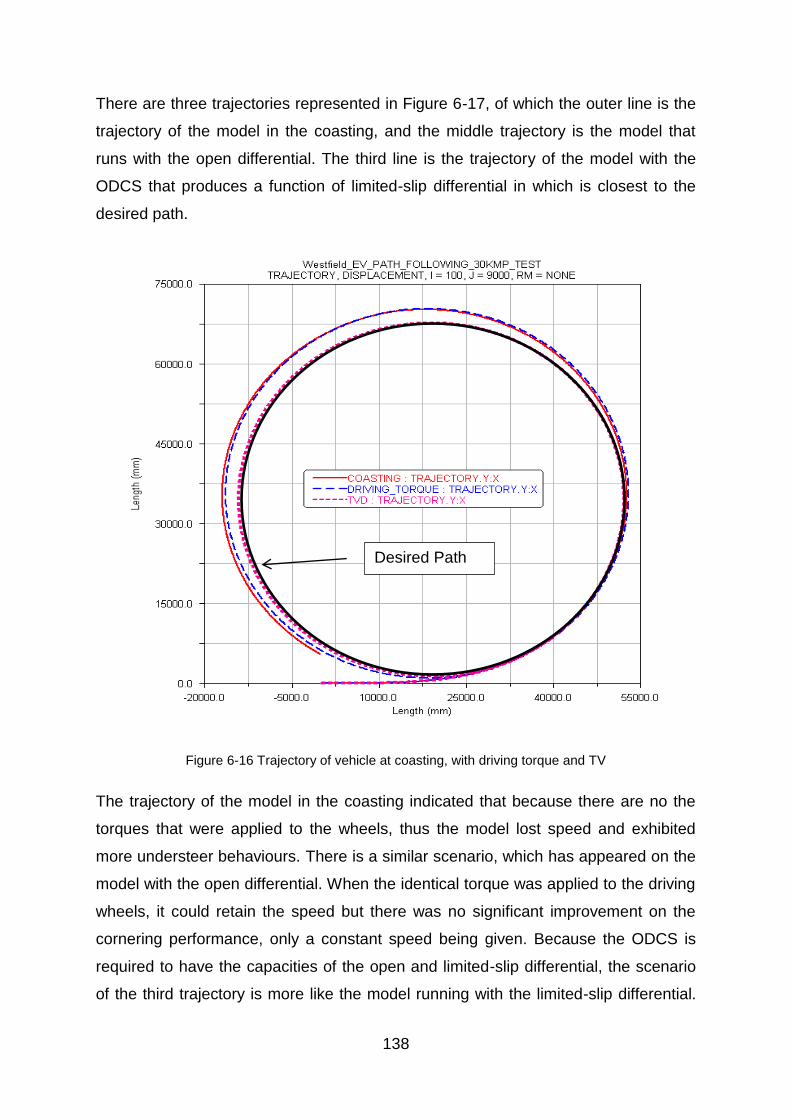
138

There are three trajectories represented in Figure 6-17, of which the outer line is the

trajectory of the model in the coasting, and the middle trajectory is the model that

runs with the open differential. The third line is the trajectory of the model with the

ODCS that produces a function of limited-slip differential in which is closest to the

desired path.

Figure 6-16 Trajectory of vehicle at coasting, with driving torque and TV

The trajectory of the model in the coasting indicated that because there are no the

torques that were applied to the wheels, thus the model lost speed and exhibited

more understeer behaviours. There is a similar scenario, which has appeared on the

model with the open differential. When the identical torque was applied to the driving

wheels, it could retain the speed but there was no significant improvement on the

cornering performance, only a constant speed being given. Because the ODCS is

required to have the capacities of the open and limited-slip differential, the scenario

of the third trajectory is more like the model running with the limited-slip differential.

Desired Path

139

The ODCS can transfer torque along the rear axle in which the difference in the

driving torque between the left and right wheels produces more yaw moment to

make the model turn more easily, to have less under-steer behaviour, and to run with

the exact desired trajectory.

Figure 6-17 Longitudinal driving forces for rear driving wheels

The measurements of the longitudinal driving force at the rear wheels are clearly

shown in Figure 6-18. The model in the coasting has none of the driving force, and

the open differential produces the identical driving force that is slightly different due

to the various vertical loads at the tyre. However, the ODCS can provide the required

driving force at each wheel, and the force is directly controlled by the PID controller

and adjusted by the ATVC. Also, it can be seen that the terms of the PID controller

produce the outputs value to reach the target proportionally around two seconds;

and then it makes some adjustment of the driving force outputs. The adjustment is

due to the desired trajectory needing some transition curvatures with varied radius to

link the path curvature from the straight line to the constant radius circle. After 4

seconds, the model has the constant driving force for turning the circle with the

constant radius.

TV right

TV left

Driving force

140

The effects on the yaw rate correction are presented in Figure 6-19. There are four

lines for describing the yaw rates of the different driving modes. The first top line is

the desired yaw rate, and the second line just below the desired yaw rate is the yaw

rate of the model with ODCS. The third line from the top is the model with the open

differential, and the bottom line is the model in the coasting condition. Obviously, the

model with the ODCS has the best result in the cornering manoeuvre. In the ODCS,

the PID controller for the yaw rate correction can reduce the error between the

desired and the actual yaw rate, and then the integral term can accelerate the

movement of the actual yaw rate towards the desired yaw rate and eliminate the

residual steady-state error that occurs from the previous proportional term. Finally,

the derivative response improves the settling time and stability of the control. It is

worth mentioning that a high proportional gain results in a large change of the output,

i.e. if the proportional gain is too high, the vehicle can become unstable. In contrast,

a small proportional gain produces a small output response to a large input error, if

the value is too low, the effects on control may not enable the enhancement of the

dynamics performance. Thus, the function of the ATVC level can solve those issues

when the PID controller is activated.

Figure 6-18 Comparison of Yaw rate correction

ODCS Desired

Yaw Rate

Coasting

With Driving Torque

Ya

w R

ate

(de

g/s

ec)

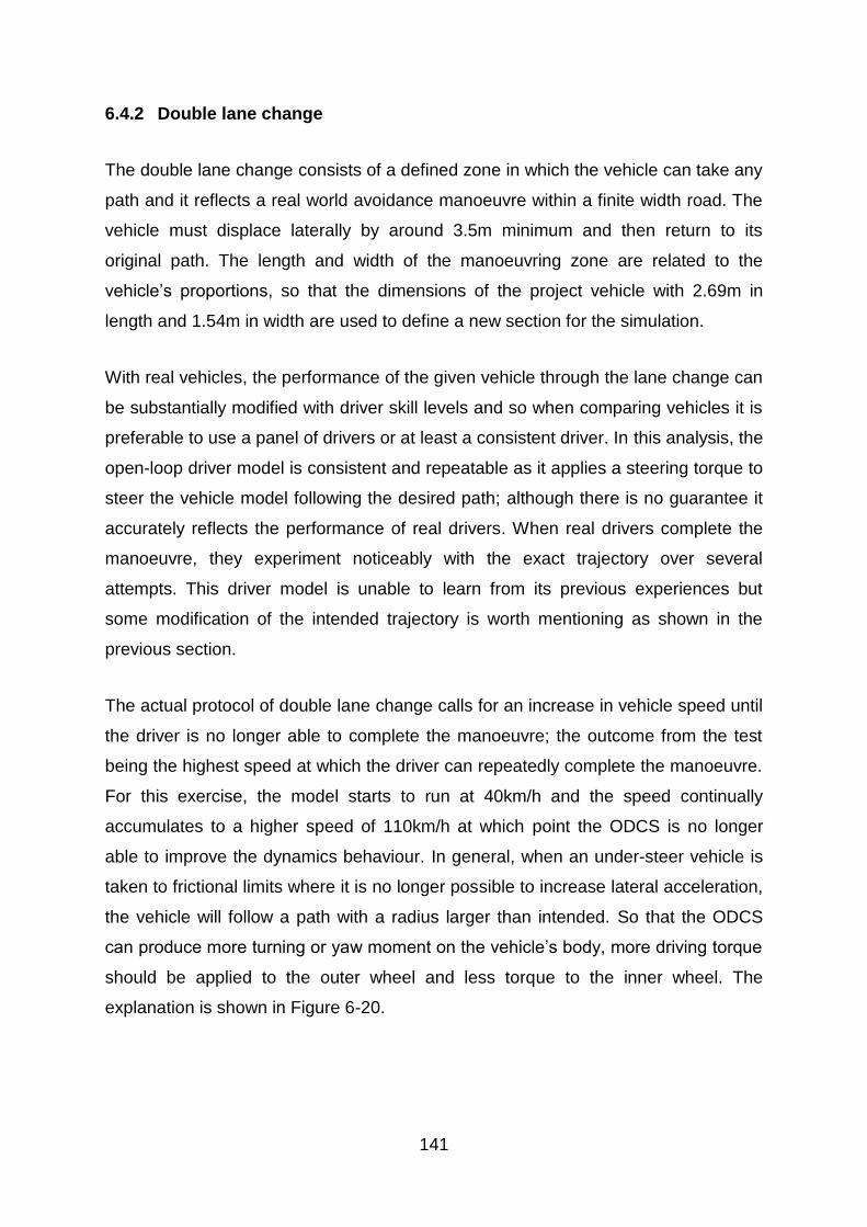
141

6.4.2 Double lane change

The double lane change consists of a defined zone in which the vehicle can take any

path and it reflects a real world avoidance manoeuvre within a finite width road. The

vehicle must displace laterally by around 3.5m minimum and then return to its

original path. The length and width of the manoeuvring zone are related to the

vehicle‘s proportions, so that the dimensions of the project vehicle with 2.69m in

length and 1.54m in width are used to define a new section for the simulation.

With real vehicles, the performance of the given vehicle through the lane change can

be substantially modified with driver skill levels and so when comparing vehicles it is

preferable to use a panel of drivers or at least a consistent driver. In this analysis, the

open-loop driver model is consistent and repeatable as it applies a steering torque to

steer the vehicle model following the desired path; although there is no guarantee it

accurately reflects the performance of real drivers. When real drivers complete the

manoeuvre, they experiment noticeably with the exact trajectory over several

attempts. This driver model is unable to learn from its previous experiences but

some modification of the intended trajectory is worth mentioning as shown in the

previous section.

The actual protocol of double lane change calls for an increase in vehicle speed until

the driver is no longer able to complete the manoeuvre; the outcome from the test

being the highest speed at which the driver can repeatedly complete the manoeuvre.

For this exercise, the model starts to run at 40km/h and the speed continually

accumulates to a higher speed of 110km/h at which point the ODCS is no longer

able to improve the dynamics behaviour. In general, when an under-steer vehicle is

taken to frictional limits where it is no longer possible to increase lateral acceleration,

the vehicle will follow a path with a radius larger than intended. So that the ODCS

can produce more turning or yaw moment on the vehicle‘s body, more driving torque

should be applied to the outer wheel and less torque to the inner wheel. The

explanation is shown in Figure 6-20.

142

Figure 6-19 Explanation of torque vectoring control at 40km/h

The project model is driven up to the manoeuvre start and the ‗throttle‘ released; the

overrun condition is typically the most difficult in terms of stability. Although the

model loses speed as it enters the second of the two manoeuvres, it is typically

unsettled dynamically and so the second transition is often the more problematic of

the two. The aim of the first run is to test what the ‗original‘ dynamics behaviour of

the model in the coasting condition is; it is also to check how the ODCS can improve

the driveability of the model in the ‗throttle off‘ condition. In Figure 6-21, the results in

the yaw rate are compared, showing a large error between the yaw rate of the model

in the coasting condition and desired yaw rate; nevertheless, the ODCS is able to

minimize the error.

Figure 6-20 Comparisons of Yaw rate without the speed controller

Desired yaw rate

With the ODCS

Coasting

143

In the second run, the speed controller is switched on to give the model traction force.

Similar results can be found in Figure 6-22 in which the ODCS can still make the

improvement in the yaw rate error correction.

Figure 6-21 Yaw rate with speed controlled

In terms of stability, reducing the body slip angle is important because it effectively

produces the width of the vehicle, and because it stores energy in the ―pendulous‖

yaw mode of vibration possessed by the running vehicle. For ordinary drivers the

storage of energy in this mode is problematic to understand and control. Figure 6-23

represents a comparison of the body slip angle for the model with the different

driving mode. In the coasting mode, the vehicle body exhibits the largest body slip

angle compared to the other two modes, and the body slip angle can be reduced

somewhat when the model runs with the driving torque. It is clear to see that the

body slip angle diminishes as the model runs with the ODCS; furthermore, the clear

improvement in the driveability can be seen throughout the trace.

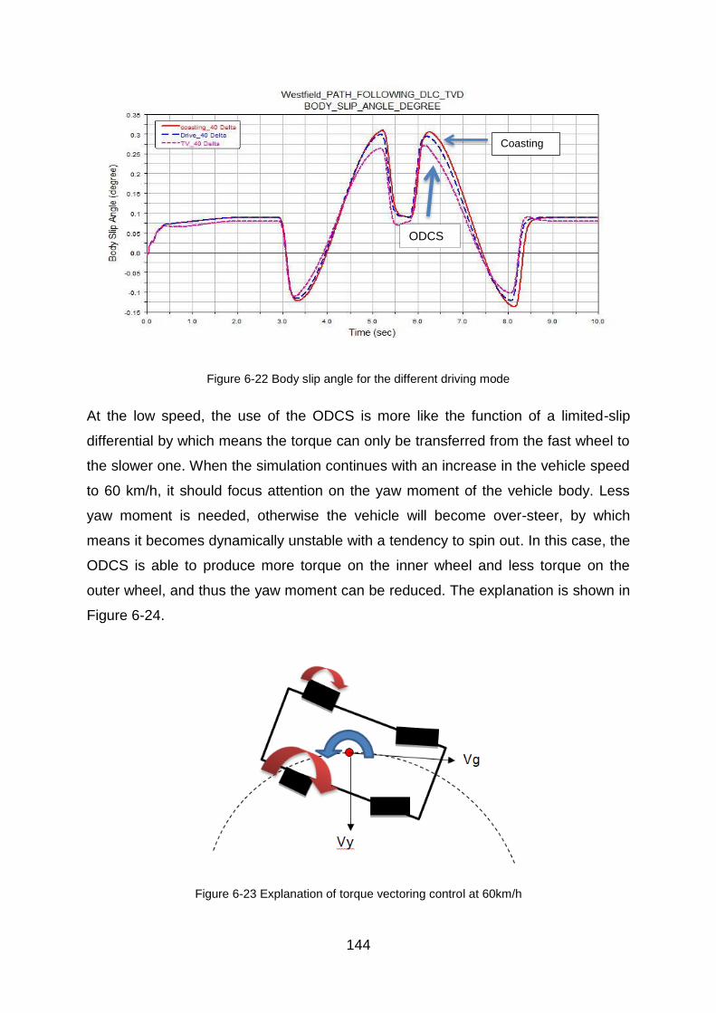
144

Figure 6-22 Body slip angle for the different driving mode

At the low speed, the use of the ODCS is more like the function of a limited-slip

differential by which means the torque can only be transferred from the fast wheel to

the slower one. When the simulation continues with an increase in the vehicle speed

to 60 km/h, it should focus attention on the yaw moment of the vehicle body. Less

yaw moment is needed, otherwise the vehicle will become over-steer, by which

means it becomes dynamically unstable with a tendency to spin out. In this case, the

ODCS is able to produce more torque on the inner wheel and less torque on the

outer wheel, and thus the yaw moment can be reduced. The explanation is shown in

Figure 6-24.

Figure 6-23 Explanation of torque vectoring control at 60km/h

ODCS

Coasting

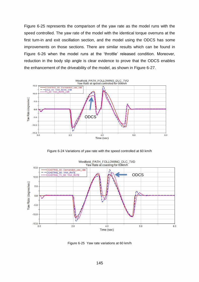
145

Figure 6-25 represents the comparison of the yaw rate as the model runs with the

speed controlled. The yaw rate of the model with the identical torque overruns at the

first turn-in and exit oscillation section, and the model using the ODCS has some

improvements on those sections. There are similar results which can be found in

Figure 6-26 when the model runs at the ‗throttle‘ released condition. Moreover,

reduction in the body slip angle is clear evidence to prove that the ODCS enables

the enhancement of the driveability of the model, as shown in Figure 6-27.

Figure 6-24 Variations of yaw rate with the speed controlled at 60 km/h

Figure 6-25 Yaw rate variations at 60 km/h

ODCS

ODCS

146

Figure 6-26 Variations of body slip angle at 60 km/h

The simulation is continued and the model is driven up to 100km/h and lateral

acceleration is about 0.65g. Figure 6-28 to 6-30 clearly show that there are some

improvements that can still be seen in the yaw rate and the body slip angle when

using the ODCS, but there are no substantial effects on the driveability. Due to the

high lateral acceleration, the model tends to be in accident-avoidance stage. Thus, it

needs to use the brakes to reduce the kinetic energy of the vehicle and to minimize

the wheel load variation for maximum grip and control. However, the limitation in the

lateral acceleration is the boundary for the operating region of the ODCS at high

speed.

Figure 6-27 Yaw rate variation at 100km/h

ODCS

147

Figure 6-28 Yaw rate variation with the speed controlled at 100km/h

Figure 6-29 Comparison of body slip angles at 100km/h

6.5 Conclusion

Based on the basic principles of torque vectoring control, the example was carried

out to explain how the mechanical TV control improves the vehicle driveability. As is

known, re-allocating the driving torque on the rear wheel results in substantial

influence on the control of the yaw moment.

There are several promising outcomes from this work listed below; these must be

interpreted in the context of the design approach used.

148

The Optimal Driveline Control Strategy (ODCS) for RWD EVs equipped with

an in-line motor at the rear wheels and the independent motor control has

been designed to enhance vehicle driveability and yaw stability.

The ODCS involves three parts: the desired dynamics behaviours, the

secondary control and the advanced torque vectoring control (ATVC). The

use of all levels has been introduced in detail, so that the desired dynamics

behaviours have been found to define the operating region and retain the

vehicle linearity. In order to track the desired dynamics, the secondary control

has been designed that can modify the traction force then to minimize the yaw

rate error and retain the vehicle speed. Since the inputs from the secondary

control should be applied to the electric motor through the ATVC, the ATVC

has been developed to map the secondary control inputs to the electric

motors.

The simulation results with the proposed driving control have been compared

to those with the two types of other driving modes in order to verify the

performance of the proposed speed control and the proposed optimal torque

vectoring algorithm. It has been shown from simulation results that the vehicle

driveability and yaw stability can be significantly improved at the same time or

individually compared to the other driving modes.

Driving control algorithms for alternative types of electric drive system, such

as a 4WD system with independently driven in-line motors, will be

investigated in the future.

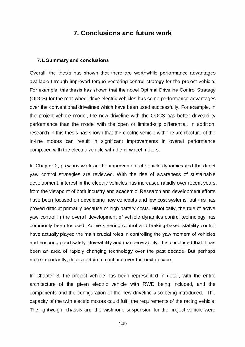
149

7. Conclusions and future work

7.1. Summary and conclusions

Overall, the thesis has shown that there are worthwhile performance advantages

available through improved torque vectoring control strategy for the project vehicle.

For example, this thesis has shown that the novel Optimal Driveline Control Strategy

(ODCS) for the rear-wheel-drive electric vehicles has some performance advantages

over the conventional drivelines which have been used successfully. For example, in

the project vehicle model, the new driveline with the ODCS has better driveability

performance than the model with the open or limited-slip differential. In addition,

research in this thesis has shown that the electric vehicle with the architecture of the

in-line motors can result in significant improvements in overall performance

compared with the electric vehicle with the in-wheel motors.

In Chapter 2, previous work on the improvement of vehicle dynamics and the direct

yaw control strategies are reviewed. With the rise of awareness of sustainable

development, interest in the electric vehicles has increased rapidly over recent years,

from the viewpoint of both industry and academic. Research and development efforts

have been focused on developing new concepts and low cost systems, but this has

proved difficult primarily because of high battery costs. Historically, the role of active

yaw control in the overall development of vehicle dynamics control technology has

commonly been focused. Active steering control and braking-based stability control

have actually played the main crucial roles in controlling the yaw moment of vehicles

and ensuring good safety, driveability and manoeuvrability. It is concluded that it has

been an area of rapidly changing technology over the past decade. But perhaps

more importantly, this is certain to continue over the next decade.

In Chapter 3, the project vehicle has been represented in detail, with the entire

architecture of the given electric vehicle with RWD being included, and the

components and the configuration of the new driveline also being introduced. The

capacity of the twin electric motors could fulfil the requirements of the racing vehicle.

The lightweight chassis and the wishbone suspension for the project vehicle were

150

described. Several sub-systems of the vehicle, for example the vehicle body, the

suspension system and the driveline, have been modelled in ADAMS, and the model

audit was carried out to ensure the reliability of the model. Also, the aerodynamic

effects were considered in this section. The driveline was able to produce the

variable driving torque at the wheels, so that it could represent the different driving

modes, such as the ‗open differential‘ and the torque vectoring control. The ‗Magic

Formula‘ tyre model was added to the vehicle model, and also used with the virtual

test rig model to examine characteristics of the tyre model in the intended behaviour

due to modifying the coefficients of the tyre model.

The analysis of the full vehicle model was presented in Chapter 4. A summary of the

simulation results was collected from these investigations to evaluate the overall

characteristics of the project model during the different analyses. First, the

characteristics of the suspension system have been determined by the kinematic

analysis in which the results can be compared with the laboratory data from

manufacturers to validate and refine the computer-based vehicle model.

Second, the dynamic analysis proved the model is a stable system with correct

degrees of freedom, the natural frequencies at each mode being calculated and the

animations clearly explaining the movement of the sprung and unsprung mass. Also

the influences of the natural frequencies at each mode were analysed. Finally, the

vehicle model ran for the characteristic driving manoeuvre - steady state cornering,

and implementing the control signal from the driver model with ‗path following‘ and

‗survey‘ controller on the steering system was represented. Of most importance is

the fact that the characteristics of the project vehicle can be defined. Furthermore,

Figure 4-23 for the yaw rate gain against the vehicle speed indicated that the aim of

the further control strategy for active yaw control is to overcome all the variations,

and then to dominate the vehicle running at its particular characteristics.

In chapter 5, the vehicle architectures of in-wheel motors and in-line motors are

introduced, and the significant modifications of original suspension have been made

to integrate all components of in-wheel motors, such as the braking system, cooling

system and electric motors, into the constrained volume at the inside of the rim.

Furthermore, the un-sprung mass is obviously increased for implementing in-wheel

151

motors on a vehicle, and degrades ride and handling performance. Compared to the

architecture of the in-wheel motors vehicle, the in-line motors vehicle required the

minimum variations of the suspension system, thus it can retain the un-sprung

masses and reduce redesign costs.

Objective measurements were carried out by using several computing simulation

models in ADAMS, such as kinematic, dynamic and handling models. The aspects of

simulation have been examined in detail and it can be concluded that the overall

performance of ride comfort is degraded, and that the obvious impact of steering

behaviour emerges with testing the vehicle models in cornering and lane change

manoeuvres. The effects on safety and driveability require some variations in

suspension component detail and increases in damping levels to restore agility.

Overall, developing the electric vehicle in its next state the architecture of the in-line

motors vehicle can preserve the characteristics of a conventional vehicle with high

performance; also, the redesign costs and efforts can be economized by improving

the capacity of the electric motors and battery life. Moreover the benefits of individual

wheel motor control can be implemented by using in-line wheel motors for

substantial improvements in vehicle behaviour.

Based on the basic principles of torque vectoring control, an example was carried

out to explain how the mechanical torque vectoring control improves the vehicle

driveability. As stated, re-allocating the driving torque on the rear wheel results in

substantial influences on the control of the yaw moment. There are several

promising outcomes from this work listed below; these must be interpreted in the

context of the design approach used.

The Optimal Driveline Control Strategy (ODCS) for RWD EVs equipped with an in-

line motor at the rear wheels and the independent motor control has been designed

to enhance vehicle driveability and yaw stability. The ODCS involves three parts: the

desired dynamics behaviours, the secondary control, and the advanced torque

vectoring control (ATVC). The use of all levels has been introduced in detail, so that

the desired dynamics behaviours have been found to define the operating region and

to retain the vehicle linearity. In order to track the desired dynamics, the secondary

152

control has been designed so that it can modify the traction force to minimize the

yaw rate error and retain the vehicle speed. Since the inputs from the secondary

control should be applied to the electric motor through the ATVC, the ATVC has

been developed to map the secondary control inputs to the electric motors.

The simulation results with the proposed driving control have been compared to

those with the other two types of driving modes in order to verify the performance of

the proposed speed control and the proposed optimal torque vectoring algorithm. It

has been shown from simulation results that the vehicle driveability and yaw stability

can be significantly improved at the same time or individually compared to the other

driving modes. Driving control algorithms for alternative types of electric drive system,

such as a 4WD system with independently driven in-line motors, will be investigated

in the future.

A procedure for the optimal PID controller design and evaluation of torque-vectoring

controller for fully electric vehicles has been presented. The results, obtained for a

vehicle with in-line motors, demonstrate the effectiveness of torque-vectoring control

in tuning vehicle response. This is achieved through a set of reference dynamics

vehicle response in conditions of constant and variable vehicle velocities. For

implementation of this torque vectoring control system, the optimal PID controller

allows to evaluate the feed forward map of the control yaw moment, as a function of

measured and estimated quantities, for a given set of vehicle and tyre parameters.

The analysis of the optimal PID control criteria shows that energy-based cost

functions provide marginal benefit in the selection of the individual wheel torque

distribution. In contrast, performance index based on driving torque output allow a

smooth variation of the wheel torques for all achievable lateral accelerations and

yield.

Overall, the novel aspects of the work are: defining the characteristics and linearity of

the project vehicle using a novel consideration of yaw rate gain; the design and

development the Optimal Driveline Control Strategy (ODCS); the analysis and

modelling the ODCS in the vehicle and the comparison of the results with

conventional drivelines. The conclusions of the research are in-line with the original

153

aim and objectives. The overall performance benefits of equipping the project vehicle

with the new control strategy have been predicted to offer significant benefits in the

dynamic control over typical driving manoeuvres.

7.2. Future work

Future work could focus on other potential benefits of vehicle dynamic control, for

instance, the driveability of an electric vehicle with individual four-wheel control. Also,

the types of subjective assessments that are used to assess driveability, for example,

the stop-start condition, the feel of acceleration or deceleration, the control pedal

response and feel, and the body slip rate control could be investigated. It is clear

there exists a research opportunity to investigate how the objective numerical

measures are relative to the subjective assessments of expert assessors, and the

effects of different architectures on drivability.

Another potential benefit of the dynamic control for the electric vehicles which could

be investigated, is whether it is possible to downsize the motor and also reduce the

weight while maintaining acceleration ability in the limited times.

The simulation in this research suggests that the idea of using an optimal control

strategy in an electric vehicle will improve the driveability performance. In future work,

a four-wheel drive model could be taken into consideration and a more complex

control strategy for individual wheel control will be developed. The research could

also be focused on attempting to quantify both driving efficiency gains and

driveability improvements.

154

Bibliography

Ackermann J, J. G. (1995). Linear and Nonlinear Controller Design for Robust

Automotive Steering. IEEE Transactions on Control Sytems Technology,

Vol.3,No.1,1995, pp. 132-143.

al., J. C. (2005). Torque Vectoring Driveline: SUV-based Demonstrator and Practical

Actuation Technologies. SAE Internationa.

Andrés Eduardo Rojas Rojas, H. N. (2010). Comfort and Safety Enhancement of

Passenger Vehicles with In-Wheel Motors. SAE International.

Andrés Eduardo Rojas Rojas, H. N. (2011). Mechanical Design of In-Wheel Motor

Driven Vehicles with Torque-Vectoring. SAE International.

Andrés Eduardo Rojas Rojas, H. N. (2011). Mechanical Design of In-Wheel Motor

Driven Vehicles with Torque-Vectoring. SAE International.

Andrés Eduardo Rojas Rojas, H. N. (2011). Mechanical Design of In-Wheel Motor

Driven Vehicles with Torque-Vectoring,. SAE International.

Assadian, F. &. (2005). A comparison of yaw stability control strategies for the active

differential. In IEEE ISIE. Dubrovnik, Croatia.

Babik, B. (2006). Advanced Technology and Energy Strategies, General Motors.

Bo rner, M. &. (2006). Model-based detection of critical driving situations with fuzzy

logic decision making. Control Engineering Practice, 14(5),527.

C Ghike, T. S. (2009). Integrated control of wheel drive–brake torque for vehicle-

handling enhancement. Proceedings of the Institution of Mechanical

Engineers, Part D: Journal of Automobile Engineering.

Chan, C. C. (2001). Modern electric vehicle technology, Oxford University Press.

Cheli, F. M. (2005). A new control strategy for a semi-active differential (Part I),. 16th

IFAC World Congress.

Colombo, D. (2005). Active differential technology for yaw moment control. In sixth

all wheel drive congress. Austria: Gratz.

155

Cong Geng, L. M. (2009). Direct Yaw-Moment Control of an In-Wheel-Motored

Electric Vehicle Based on Body Slip Angle Fuzzy Observer. IEEE

TRANSACTIONS ON INDUSTRIAL ELECTRONICS, VOL. 56, NO. 5,.

Edoardo Sabbioni, L. K. (2010). On the Impact of the Maximum Available Tire-Road

Friction Coefficient Awareness in a Brake-Based Torque Vectoring System.

SAE International.

Edoardo Sabbioni, L. K. (2010). On the Impact of the Maximum Available Tire-Road

Friction Coefficient Awareness in a Brake-Based Torque Vectoring System.

SAE International.

ExxonMobil. (2007). New Outlook for Energy: A View to 2030. Texas, ExxonMobil.

F. Assadian, M. H. (2008). Development of a Control Algorithm for an Active Limited

Slip Differential. Loughborough University / Society of Automotive Engineers

of Japan (JSAE).

F. Cheli, M. P. (2006). Development of a new control strategy for a semi-active

differential for a high-performance vehicle. Vehicle System Dynamics - VEH

SYST DYN 01/2006; 44:202-215. .

G. Kaiser, F. H. (2011). Torque Vectroing with a feedback and feed forward

controller - applied to a through the road vehicle. IEEE Intelligent Vehicle

Symposium.

Gaspar, P. S. (2005). Reconfigurable control structure to prevent the rollover of

heavy vehicles. Control Engineering Practice, 13(6), 699.

Gerd Kaiser, F. H. (2011). Torque Vectoring with a feedback and feed forward

controller - applied to a through the road hybrid electric vehicle. IEEE.

Gerhard, J. L.-C. (2005). Robust yaw control design with active differential and active

roll control systems. In 16th IFAC world congress. Prague, Czech Republic.

Gillespie, T. D. (1992). Fundamentals of Vehicle Dynamics. SAE International.

156

Göschel, B. (2008). Ausgewählte Kapitel der Verbrennungskraftmaschinen:

Alektrifizierung Antrieb. Institute for Internal Combustion Engines and

Thermodynamics, Graz University of Technology.

Harty, M. B. (2004). Multibody Systems Approach to Vehicle Dynamics. Elsevier‘s

Science and Technology Rights Department.

Hirsch, R. L. (2005). Peaking of World Oil Production: Impacts, Mitigation & Risk

Management.

Husain, I. (2003). Electric and hybrid vehicles; design fundamentals., CRC Press.

Ikushima, Y. a. (1995). "A Study on the Effects of the Active Yaw Moment Control,".

SAE Technical Paper 950303, 1995, doi:10.4271/950303.

IME. (2009). Brochure for Integrating Technologies for Low Carbon. Integrating

Technologies for Low Carbon, Norfolk, Institution of Mechanical Engineers.

Inoue, K. S. (2007). Effect of the Right-and-left Torque Vectoring System in Various

Types of Drivetrain. SAE International, 2007-01-3645.

IPIECA. (2004). Transportation and climate change: opportunities, challenges and

longterm strategies. AN IPECA workshop, Baltimore, USA.

J.C. Wheals, M. D. (2006). Design and Simulation of a Torque Vectoring™Rear Axle.

SAE International.

Johann Willberger, M. A. (2010). Motor Selection Criteria and Potentials of Electrified

All Wheel Drive Concepts for Passenger Cars by Add-on Wheel Hub Motors

on the Rear Axle. SAE International.

Johann Willberger, M. A. (2010). Motor Selection Criteria and Potentials of Electrified

All Wheel Drive Concepts for Passenger Cars by Add-on Wheel Hub Motors

on the Rear Axle. SAE International.

Johann Willberger, M. A. (2010). Motor Selection Criteria and Potentials of Electrified

All Wheel Drive Concepts for Passenger Cars by Add-on Wheel Hub Motors

on the Rear Axle. SAE International .

157

John Feltman, J. G. (2006). Mechatronic Torque Vectoring System with Enhanced

Controllability for Augmenting the Vehicle Agility and Safety. SAE

International.

Jonathan C. Wheals, H. B. (2004). Torque Vectoring AWD Driveline: Design,

Simulation, Capabilities and Control. SAE International ISBN 0-7680-1319-4.

Jonathan C. Wheals, H. B. (2004). Torque Vectoring AWD Driveline:

Design,Simulation, Capabilities and Control. SAE International.

Juyong Kang, Y. k. (2012). Control Allocation based Optimal Torque Vectoring for

4WD Electric Vehicle. SAE International.

Kakalis L., C. F. (2010). n the impact of the maximum available tire-road friction

coefficient awareness in a brake-based torque vectoring system. . In SAE

International Congress and Exposition, SAE Paper 2010-01-0116.

Kang, J. k. (2012). Control Allocation based Optimal Torque Vectoring for 4WD

Electric Vehicle. SAE Technical Paper 2012-01-0246.

Kim, D.-H. J. (2007). "Optimal brake torque distribution for a four-wheel drive hybrid

electric vehicle stability enhancement." . Proc. IMechE, Part D: J Automobile

Engineering vol. 221: 1357-1366.

Kiumars Jalali, K. B. (2008). Design of an Advanced Traction Controller for an

Electric Vehicle Equipped with Four Direct Driven In-Wheel Motors. SAE

International.

Kiumars Jalali, T. U. (2012). Development of a Fuzzy Slip Control System for Electric

Vehicles with In-wheel Motors. SAE International.

Kohen, P. &. (2004). Active steering—the BMW approach towards modern steering

technology. . In SAE Technical Paper No.2004-01-1105.

Kroppe, J. P. (2004). Dana Torque Vectoring Differential Dynamic Trak. SAE

International.

Larminie, J. a. (2003). Electric vehicle technology explained. West Sussex, England,

J. Wiley.

158

Lifu Li, Z. (2011). Study on Torque Vectoring Differential for Vehicle Stability Control

via Hardware Hardwarein-. IEEE.

M Milehins, C. C. (2010). Handling behaviour of a TTR hybrid electric vehicle with

independent rear wheel torque control. In: AVEC10.

Martyn Anderson, D. H. (2011). Unsprung Mass with In-Wheel Motors - Myths and

Realities. SAE International .

Milliken, W. a. (1995). Race car vehicle dynamics. Society of Automotive Engineers,

Inc .

Mokhiamar, O. &. (2002). Active wheel steering and yaw moment control

combination to maximize stability as well as responsiveness during quick lane

change for active vehicle handling safety. Proceedings of the Institution of

Mechanical Engineers Part D, Journal of Automobile Engineering, 216(1),

115–124.

Motoki Shino, M. N. (2001). Yaw-moment control of electric vehicle for improving

handling and stability. Society of Automotive Engineers of Japan, Inc. and

Elsevier Science B.V.

Neudorfer, H., Binder, A., & Wicker, N. (2006). Analyse von Unterschiedlichen

Fahrzyklen fur den einsatz von Elektrofahrzeugen . E&I 123 no 7-8 p,352-360.

O‘Hara, S. R. (2005). VEHICLE PATH OPTIMIZATION OF EMERGENCY LANE

CHANGE MANEUVERS FOR VEHICLE SIMULATION.

Pacejka, H. a. (1991). Shear force generation by pneumatic tyres in steady state

conditions: a review of modelling aspects. Vehicle System Dynamics, 20, pp.

121–176, 1991.

PINTO, L. A. (2011). YAW MOTION CONTROL OF A VEHICLE. International Patent

Cooperation Treaty.

Qin Liu, G. K. (2011). Two-Degree-of-Freedom LPV Control for a through-the-Road

Hybrid Electric Vehicle via Torque Vectoring. IEEE.

159

Randall, B. P. (2009). Electric cars - are they really 'green'? Low-carbon vehicles

2009, London, Institution of Mechanical Engineers.

Resta, F. G. (2005). A new control strategy of a semi-active differential (Part II). the

16th IFAC WORLD CONGRESS.

Sawase, K. U. (2007). Effect of the Right-and-left Torque Vectoring System in

Various Types of Drivetrain. SAE Technical Paper 2007-01-3645, 2007,

doi:10.4271/2007-01-3645.

Sawase, T. K. (2012). Classification and analysis of electric Classification and

analysis of electricpowered. Proceedings of the Institution of Mechanical

Engineers, Part D: Journal of Automobile Engineering.

Sharma, S. K. (2006). Torque Vectoring Axle and Four Wheel Steering: A Simulation

Study of Two Yaw Moment Generation Mechanisms. SAE International.

Sharma, S. K. (2006). Torque Vectoring Axle and Four Wheel Steering: A Simulation

Study of Two Yaw Moment Generation Mechanisms. SAE International.

Sharma, S. K. (2006). Torque Vectoring Axle and Four Wheel Steering: A Simulation

Study of Two Yaw Moment Generation Mechanisms. SAE International.

Sienel, A. J. (1993). Robust Yaw and Damping of Cars with Front and Rear Wheel

Steering. IEEE Transactions on Control Systems Technology,

Vol.1,No.1,1993,pp.15-20.

Taehyun Shim, G. A. (n.d.). Autonomous vehicle collision avoidance system using

path planning and model-predictive-control-based active front steering and

wheel torque control. Proceedings of the Institution of Mechanical Engineers,

Part D: Journal of Automobile Engineering.

Taeyoung Lee, J. K. (2010). Integration of Longitudinal and Lateral Human Driver

Models for Evaluation of the Vehicle Active Safety Systems. SAE International.

van Zanten, A. T. (1995). VDC, the vehicle dynamics control system of bosch. In

SAE Technical Paper No. 95759.

160

van Zanten, A. T. (2000). Bosch ESP systems: 5 years of experience. In SAE

Technical Paper No. 2000-01-1633.

Vilaplana, M. A. (2005). Control of yaw rate and sideslip in 4-wheel steering cars with

actuator constraints. Lecture Notes in Computer Science, (vol. 3355, pp.201–

222). Berlin: Springer.

Whitehead, A. (2012). IN-WHEEL ELECTRIC MOTORS. The Packaging and

Integration Challenges Senior Mechanical Systems Engineer Protean Electric

Ltd, UK, p. 15.

Wu, L. L. (2011). Study on Torque Vectoring Differential for Vehicle Stability Control

via Hardware-in-Loop Simulation. IEEE 978-1-61284-486-2/111.

YASA motor. (2014). Retrieved from http://www.yasamotors.com/technology

Zhang, Y. H. (2006). "Performance modelling and optimization of a novel multi mode

hybrid powertrain.". Trans. ASME, J. Mech. Design 128(1): 79-89.

161

Appendix

Appendix 1 Westfield vehicle model for kinematic analysis (part of the model)

!-------------------------- Default Units for Model ---------------------------! defaults units & length = mm &angle = deg & force = newton mass = kg &time = sec defaults units & coordinate_system_type = cartesian & orientation_type = body313 !------------------------ Default Attributes for Model ------------------------! defaults attributes & inheritance = bottom_up &icon_visibility = on grid_visibility = off & size_of_icons = 20.0 & spacing_for_grid = 1000.0 !------------------------------ Adams/View Model ------------------------------! model create &model_name = Westfield_Front_Drive_Kin_rig model attributes model_name = Westfield_Front_Drive_Kin_rig & size_of_icons = 20.0 view erase -------------------------------- Materials ----------------------------------! material create & material_name = .Westfield_Front_Drive_Kin_rig.steel & adams_id = 1 &youngs_modulus = 2.07E+005 &poissons_ratio = 0.29 & density = 7.801E-006 !-------------------------------- Rigid Parts ---------------------------------! ! Create parts and their dependent markers and graphics !----------------------------------- ground -----------------------------------! ! ****** Ground Part ****** defaults model &part_name = grounddefaults coordinate_system & default_coordinate_system = .Westfield_Front_Drive_Kin_rig.ground ! ****** Markers for current part ****** marker create & marker_name = .Westfield_Front_Drive_Kin_rig.ground.m_wheel_centre_ground adams_id = 2 & location = -1167.999, 663.971, 0.0 & orientation = 0.0d, 0.0d, 0.0d marker attributes &marker_name = m_wheel_centre_ground &size_of_icons = 20.0 marker create &marker_name = .Westfield_Front_Drive_Kin_rig.ground.MARKER_57 & adams_id = 57 & location = -1269.8, 336.933, -96.75 &orientation = 186.7030013032d, 79.0487029613d, 0.0 marker create &marker_name = .Westfield_Front_Drive_Kin_rig.ground.Body_FD_Lower_wish_rev_joint_maker & adams_id = 42 & location = -1026.439, 190.41, -135.4 & orientation = 269.7809583075d, 90.0d, 0.0d marker create &marker_nam = .Westfield_Front_Drive_Kin_rig.ground.MARKER_55 & adams_id = 55 &location = -1183.751, 279.455, 121.4 &orientation = 0.0d, 0.0d, 0.0d marker create marker_name = .Westfield_Front_Drive_Kin_rig.ground.MARKER_63 adams_id = 63 & location = -1183.751, 279.455, 121.4 &orientation = 178.4831821016d, 136.0112734674d, 0.0d marker create &marker_name = .Westfield_Front_Drive_Kin_rig.ground.MARKER_99 & adams_id = 99 & location = -1277.559, 290.911, 74.56 &orientation = 270.1944385707d, 90.0d, 90.0d marker create &marker_name = .Westfield_Front_Drive_Kin_rig.ground.MARKER_80 & adams_id = 80 location = -1167.999, 663.971, -50.0 & orientation = 0.0d, 0.0d, 0.0d marker create & marker_name = .Westfield_Front_Drive_Kin_rig.ground.ground_wheel_base &adams_id = 88 & location = -1167.999, 663.971, -266.0 &orientation = 0.0d, 0.0d, 0.0d marker create &marker_name = .Westfield_Front_Drive_Kin_rig.ground.MARKER_108 &adams_id = 108 &location = -1167.999, 663.971, -200.0 &orientation = 0.0d, 0.0d, 0.0d part create rigid_body mass_properties part_name= .Westfield_Front_Drive_Kin_rig.ground &material_type = .Westfield_Front_Drive_Kin_rig.steel ! ****** Points for current part ******

162

point create &point_name = .Westfield_Front_Drive_Kin_rig.ground.upper_wishbone_outer_ball_joint & location = -1158.169, 551.78, 74.5point attributes &point_name = upper_wishbone_outer_ball_joint & size_of_icons = 20.0 ! point create &point_name = .Westfield_Front_Drive_Kin_rig.ground.upper_wishbone_inner_Rear_joint &location = -1085.433, 291.563, 74.5 point create & point_name= .Westfield_Front_Drive_Kin_rig.ground.upper_wishbone_inner_Front_joint &location = -1277.559, 290.911, 74.56 point attributes & point_name = upper_wishbone_inner_Front_joint &size_of_icons = 20.0 point create & point_name = .Westfield_Front_Drive_Kin_rig.ground.POINT_25 & location = -1050.0, 350.0, 0.0 point create & point_name = .Westfield_Front_Drive_Kin_rig.ground.lower_wishbone_outer_ball_joint & location = -1177.704, 570.758, -135.4 point attributes point_name = lower_wishbone_outer_ball_joint &size_of_icons = 20.0 !----------------------------- FD_Upper_wishbone ------------------------------ defaults coordinate_system &default_coordinate_system = .Westfield_Front_Drive_Kin_rig.ground part create rigid_body name_and_position &part_name = .Westfield_Front_Drive_Kin_rig.FD_Upper_wishbone & adams_id = 8 & location = 0.0, 0.0, 0.0 & orientation = 0.0d, 0.0d, 0.0d part create rigid_body initial_velocity & part_name = .Westfield_Front_Drive_Kin_rig.FD_Upper_wishbone &vx = -2.7778E+004 defaults coordinate_system & default_coordinate_system = .Westfield_Front_Drive_Kin_rig.FD_Upper_wishbone ! ****** Markers for current part ****** marker create &marker_name = .Westfield_Front_Drive_Kin_rig.FD_Upper_wishbone.MARKER_98 &adams_id = 98 location = -1277.559, 290.911, 74.56 & orientation = 270.1944385707d, 90.0d, 90.0 marker create & marker_name = .Westfield_Front_Drive_Kin_rig.FD_Upper_wishbone.MARKER_35 adams_id = 35 & location = -1085.433, 291.563, 74.56 & orientation = 65.4081991848d, 0.0d, 0.0 !----------------------------- FD_Lower_wishbone ------------------------------! defaults coordinate_system &default_coordinate_system = .Westfield_Front_Drive_Kin_rig.ground part create rigid_body name_and_position & part_name = .Westfield_Front_Drive_Kin_rig.FD_Lower_wishbone & adams_id = 7 & location = 0.0, 0.0, 0.0 & orientation = 0.0d, 0.0d, 0.0d part create rigid_body initial_velocity & part_name = .Westfield_Front_Drive_Kin_rig.FD_Lower_wishbone &vx = -2.7778E+004 defaults coordinate_system &default_coordinate_system = .Westfield_Front_Drive_Kin_rig.FD_Lower_wishbone ! ****** Markers for current part ****** marker create & marker_name = .Westfield_Front_Drive_Kin_rig.FD_Lower_wishbone.MARKER_30 adams_id = 30 & location = -1177.704, 570.758, -135.4 & orientation = 291.6877938567d, 0.0d, 0.0d marker create &marker_name= .Westfield_Front_Drive_Kin_rig.FD_Lower_wishbone.MARKER_31 &adams_id = 31 & location = -1026.439, 190.41, -135.4 & orientation = 291.6877938567d, 0.0d, 0.0d marker create &marker_name = .Westfield_Front_Drive_Kin_rig.FD_Lower_wishbone.cm & adams_id = 43 & location = -1179.1194902269, 380.878555804, -135.4 & orientation = 179.2773770674d, 90.0000000007d, 89.9999999907d

163

marker create &marker_name = .Westfield_Front_Drive_Kin_rig.FD_Lower_wishbone.MARKER_32 adams_id = 32 & location = -1177.704, 570.758, -135.4 & orientation = 291.6877938567d, 0.0d, 0.0d marker create & marker_name = .Westfield_Front_Drive_Kin_rig.FD_Lower_wishbone.MARKER_33 & adams_id = 33 & location = -1334.311, 191.587, -135.4 orientation = 291.6877938567d, 0.0d, 0.0

marker create & marker_name = .Westfield_Front_Drive_Kin_rig.FD_Lower_wishbone.FD_Lower_wish_rev_joint_marker &adams_id = 41 & location = -1026.439, 190.41, -135.4 & orientation = 269.7809583075d, 90.0d, 0.0d !

marker create & marker_name = .Westfield_Front_Drive_Kin_rig.FD_Lower_wishbone.lower_wishbone_ball_joint & adams_id = 47 & location = -1177.704, 570.758, -135.4 & orientation = 0.0d, 0.0d, 0.0d ! marker create & marker_name = .Westfield_Front_Drive_Kin_rig.FD_Lower_wishbone.MARKER_70 & adams_id = 70 & location = -1178.278, 486.142, -92.79 & orientation = 0.0d, 0.0d, 0.0d ! part create rigid_body mass_properties & part_name = .Westfield_Front_Drive_Kin_rig.FD_Lower_wishbone & mass = 2.497681221 & center_of_mass_marker = & .Westfield_Front_Drive_Kin_rig.FD_Lower_wishbone.cm & ixx = 5.130318723E+004 & iyy = 3.158268078E+004 & izz = 1.984539051E+004 & ixy = 0.0 & izx = 0.0 & iyz = 0.0 ! ****** Graphics for current part ******

geometry create shape link & link_name = .Westfield_Front_Drive_Kin_rig.FD_Lower_wishbone.LINK_19 & i_marker = .Westfield_Front_Drive_Kin_rig.FD_Lower_wishbone.MARKER_30 & j_marker = .Westfield_Front_Drive_Kin_rig.FD_Lower_wishbone.MARKER_31 & width = 40.0 & depth = 20.0 !

geometry create shape link & link_name = .Westfield_Front_Drive_Kin_rig.FD_Lower_wishbone.LINK_20 & i_marker = .Westfield_Front_Drive_Kin_rig.FD_Lower_wishbone.MARKER_32 & j_marker = .Westfield_Front_Drive_Kin_rig.FD_Lower_wishbone.MARKER_33 & width = 40.0 &

depth = 20.0

part attributes & part_name = .Westfield_Front_Drive_Kin_rig.FD_Lower_wishbone & color = MAIZE & name_visibility = off

164

!---------------------------------- upright -----------------------------------!

defaults coordinate_system & default_coordinate_system = .Westfield_Front_Drive_Kin_rig.ground ! part create rigid_body name_and_position & part_name = .Westfield_Front_Drive_Kin_rig.upright & adams_id = 4 & location = 0.0, 0.0, 0.0 & orientation = 0.0d, 0.0d, 0.0d part create rigid_body initial_velocity & part_name = .Westfield_Front_Drive_Kin_rig.upright & vx = -2.7778E+004 ! defaults coordinate_system & default_coordinate_system = .Westfield_Front_Drive_Kin_rig.upright ! ****** Markers for current part ****** marker create & marker_name = .Westfield_Front_Drive_Kin_rig.upright.MARKER_34 & adams_id = 34 & location = -1167.999, 663.971, 0.0 & orientation = 0.0d, 90.0d, 0.0d !

marker create & marker_name = .Westfield_Front_Drive_Kin_rig.upright.m_upright_CG & adams_id = 17 & location = -1167.999, 561.269, 0.0 & orientation = 0.0d, 0.0d, 0.0d !

marker attributes & marker_name = m_upright_CG & size_of_icons = 20.0 ! marker create & marker_name = .Westfield_Front_Drive_Kin_rig.upright.m_upright_graphics & adams_id = 18 & location = -1177.704, 570.758, -135.4 & orientation = 45.8285909785d, 7.391038812d, 313.9325193345d ! marker attributes & marker_name = m_upright_graphics & size_of_icons = 20.0 !

marker create & marker_name = .Westfield_Front_Drive_Kin_rig.upright.m_upright_graphics2 & adams_id = 19 & location = -1298.093, 577.671, -49.847 & orientation = 82.8141733619d, 69.1856027052d, 272.5651822746d

Appendix 2 Westfield model for Eigen solution ( part of model) !-------------------------- Default Units for Model ---------------------------! defaults units & length = mm &

165

angle = deg & force = newton & mass = kg & time = sec ! defaults units & coordinate_system_type = cartesian & orientation_type = body313 ! !------------------------ Default Attributes for Model ------------------------! defaults attributes & inheritance = bottom_up & icon_visibility = on & grid_visibility = off & size_of_icons = 20.0 & spacing_for_grid = 1000.0 ! !------------------------------ Adams/View Model ------------------------------! model create & model_name = Westfield_full_vehicle_Eigen ! model attributes & model_name = .Westfield_full_vehicle_Eigen & size_of_icons = 20.0 ! view erase !-------------------------------- Data storage --------------------------------! data_element create variable & variable_name = .Westfield_full_vehicle_Eigen.YAW_RATE_VAR & adams_id = 25136 & initial_condition = 0.0 & function = "" ! data_element create spline & spline_name = .Westfield_full_vehicle_Eigen.SPLINE_G686 & adams_id = 1000 & comments = "DAMPER SPLINES", "G686 WESTFIELD 3742078" & x = -2000.0, -840.995, -800.995, -760.995, -720.995, -680.995, -660.995, & -580.995, -520.995, -460.995, -420.995, -380.995, -340.995, -300.995, & -270.995, -240.995, -228.995, -207.995, -192.887, -174.38, -161.916, & -144.542, -128.301, -113.57, -98.84, -85.998, -71.268, -57.293, & -43.696, -27.455, -15.746, 0.0, 15.746, 27.455, 38.408, 47.851, & 53.894, 64.092, 75.045, 83.354, 90.153, 100.728, 112.059, 122.257, & 130.944, 140.765, 152.096, 161.16, 167.959, 176.646, 184.2, 193.265, & 204.974, 214.974, 224.974, 234.974, 244.974, 254.974, 264.974, & 274.974, 284.974, 294.974, 304.974, 314.974, 380.0 & y = 2000.0, 1186.0, 1156.0, 1126.0, 1096.0, 1066.0, 1036.0, 1006.0, 976.0, & 946.0, 916.0, 886.0, 856.0, 826.0, 796.0, 766.0, 736.0, 706.522, & 670.29, 634.058, 606.884, 570.652, 525.362, 498.188, 461.956, 434.782, & 389.493, 362.319, 317.029, 262.681, 226.449, 0.0, -280.797, -452.899, & -625.0, -778.986, -878.623, -996.377, -1105.073, -1195.652, -1277.174, & -1385.87, -1494.565, -1603.261, -1702.899, -1802.536, -1938.406, & -2028.986, -2110.507, -2255.435, -2391.304, -2536.232, -2726.449, & -2926.0, -3126.0, -3326.0, -3526.0, -3726.0, -3926.0, -4126.0, & -4326.0, -4526.0, -4726.0, -4926.0, -8000.0 & linear_extrapolate = no ! data_element attributes & data_element_name = .Westfield_full_vehicle_Eigen.SPLINE_G686 & visibility = off

166

! data_element create spline & spline_name = .Westfield_full_vehicle_Eigen.SPLINE_West_1 & adams_id = 2000 & comments = "WESTFIELD 1" & x = -1000.0, -273.24, -262.24, -251.24, -240.24, -229.24, -218.24, & -207.24, -196.287, -182.689, -170.603, -157.006, -143.031, -130.189, & -118.858, -104.128, -87.131, -78.067, -69.002, -58.048, -41.807, & -29.343, -16.124, 0.0, 16.124, 35.764, 48.606, 60.315, 70.135, 80.333, & 90.153, 101.484, 110.549, 120.369, 131.7, 144.919, 157.383, 174.38, & 186.089, 197.797, 206.484, 216.0, 226.0, 236.0, 250.0, 267.0, 520.0 & y = 2400.0, 750.0, 720.0, 690.0, 660.0, 630.0, 600.0, 588.768, 570.652, & 534.42, 507.246, 498.188, 461.956, 434.782, 416.667, 371.377, 335.145, & 317.029, 289.855, 262.681, 199.275, 153.985, 108.696, 0.0, -63.406, & -217.391, -326.087, -434.783, -525.362, -625.0, -724.638, -824.276, & -896.739, -969.203, -1068.841, -1186.594, -1277.174, -1422.102, & -1530.797, -1630.435, -1702.899, -1772.0, -1870.0, -1970.0, -2100.0, & -2200.0, -5000.0 & linear_extrapolate = no ! data_element attributes & data_element_name = .Westfield_full_vehicle_Eigen.SPLINE_West_1 & visibility = off ! data_element create spline & spline_name = .Westfield_full_vehicle_Eigen.SPLINE_West_2 & adams_id = 3000 & comments = "WESTFIELD 2" & x = -1000.0, -272.995, -251.995, -239.995, -228.995, -215.995, -201.952, & -187.222, -170.603, -156.628, -142.653, -131.322, -118.103, -104.883, & -92.041, -81.088, -71.268, -60.692, -50.117, -38.03, -25.944, -15.746, & 0.0, 15.746, 25.566, 36.52, 47.473, 53.894, 60.315, 68.624, 79.955, & 90.153, 99.973, 109.793, 119.613, 128.678, 137.743, 149.829, 159.65, & 170.603, 180.423, 192.51, 206.484, 212.484, 231.0, 251.0, 272.0, & 1000.0 & y = 1448.5058131529, 601.0, 584.0, 551.0, 519.0, 498.188, 489.13, 461.956, & 434.782, 407.609, 380.435, 353.261, 326.087, 298.913, 271.739, & 235.507, 217.391, 190.217, 163.043, 135.869, 108.696, 90.58, 0.0, & -36.232, -63.406, -90.58, -117.754, -135.87, -181.16, -217.391, & -280.797, -344.203, -407.609, -471.015, -543.478, -606.884, -670.29, & -751.812, -806.16, -878.623, -951.087, -1032.609, -1114.131, -1210.0, & -1290.0, -1410.0, -1580.0, -6756.1418342369 & linear_extrapolate = no ! data_element attributes & data_element_name = .Westfield_full_vehicle_Eigen.SPLINE_West_2 & visibility = off ! data_element create spline & spline_name = .Westfield_full_vehicle_Eigen.LEFT_TURN_SPLINE & adams_id = 7000 & x = 0.0, 8.333, 16.666, 21.5, 24.999, 33.332, 41.665, 49.998, 58.331, & 63.0, 66.664, 74.997, 83.33, 91.663, 99.996, 108.329, 116.662, & 124.995, 133.328, 141.661, 149.994, 158.327, 166.66, 174.993, 183.326, & 191.659, 199.992, 208.325, 216.658, 224.991, 233.324, 241.657, 249.99, & 258.323, 266.656, 274.989, 283.322, 291.655, 299.988, 308.321, & 316.654, 324.987, 333.32, 341.653, 349.986, 358.319, 366.652, 374.985, & 383.318, 391.651, 399.984, 408.317, 416.65, 424.983, 433.316, 441.649, & 449.982, 458.315, 466.648, 474.981, 483.314, 491.647 & y = 0.0, 0.0, -1.0E-003, -2.7575744042E-003, -5.05E-003, -1.01E-002, &

167

-1.515E-002, -2.02E-002, -2.4997042955E-002, -2.7618766292E-002, & -2.9065236397E-002, -2.9969280214E-002, -3.03E-002, -3.03E-002, & -3.03E-002, -3.03E-002, -3.03E-002, -3.03E-002, -3.03E-002, & -3.03E-002, -3.03E-002, -3.03E-002, -3.03E-002, -3.03E-002, & -3.03E-002, -3.03E-002, -3.03E-002, -3.03E-002, -3.03E-002, & -3.03E-002, -3.03E-002, -3.03E-002, -3.03E-002, -3.03E-002, & -3.03E-002, -3.03E-002, -3.03E-002, -3.03E-002, -3.03E-002, & -3.03E-002, -3.03E-002, -3.03E-002, -3.03E-002, -3.03E-002, & -3.03E-002, -3.03E-002, -3.03E-002, -3.03E-002, -3.03E-002, & -3.03E-002, -3.03E-002, -3.03E-002, -3.03E-002, -3.03E-002, & -3.03E-002, -3.03E-002, -3.03E-002, -3.03E-002, -3.03E-002, & -3.03E-002, -3.03E-002, -3.03E-002 & linear_extrapolate = yes ! data_element attributes & data_element_name = .Westfield_full_vehicle_Eigen.LEFT_TURN_SPLINE & visibility = off !--------------------------------- Materials ---------------------------------- material create & material_name = .Westfield_full_vehicle_Eigen.steel & adams_id = 1 & youngs_modulus = 2.07E+005 & poissons_ratio = 0.29 & density = 7.801E-006 !-------------------------------- Rigid Parts ---------------------------------! ! ! Create parts and their dependent markers and graphics ! !----------------------------------- ground -----------------------------------! ! ****** Ground Part ****** defaults model & part_name = ground defaults coordinate_system & default_coordinate_system = .Westfield_full_vehicle_Eigen.ground ! ****** Markers for current part ****** marker create & marker_name = .Westfield_full_vehicle_Eigen.ground.m_wheel_centre_ground & adams_id = 2 & location = -1167.999, 663.971, 0.0 & orientation = 0.0d, 0.0d, 0.0d ! marker attributes & marker_name = .Westfield_full_vehicle_Eigen.ground.m_wheel_centre_ground & size_of_icons = 20.0 ! marker create & marker_name = .Westfield_full_vehicle_Eigen.ground.MARKER_150 & adams_id = 150 & location = 1163.586, 399.311, 419.149 & orientation = 0.0d, 0.0d, 0.0d ! marker create & marker_name = .Westfield_full_vehicle_Eigen.ground.ground_wheel_base & adams_id = 200 & location = 1169.081, 663.971, -266.0 & orientation = 0.0d, 0.0d, 0.0d ! marker create & marker_name = .Westfield_full_vehicle_Eigen.ground.MARKER_292 &

168

adams_id = 292 & location = 1163.586, -399.311, 419.149 & orientation = 0.0d, 0.0d, 0.0d ! marker create & marker_name = .Westfield_full_vehicle_Eigen.ground.MARKER_342 & adams_id = 342 & location = -1334.311, 191.587, -255.4 & orientation = 0.0d, 0.0d, 0.0d ! marker create & marker_name = .Westfield_full_vehicle_Eigen.ground.MARKER_369 & adams_id = 369 & location = 993.63, 134.002, -255.4 & orientation = 0.0d, 0.0d, 0.0d ! marker create & marker_name = .Westfield_full_vehicle_Eigen.ground.MARKER_404 & adams_id = 404 & location = -1269.8, 336.933, -33.12 & orientation = 0.0d, 0.0d, 0.0d ! marker create & marker_name = .Westfield_full_vehicle_Eigen.ground.aero_drag_marker & adams_id = 405 & location = -1.00964, 0.0, -33.7444 & orientation = 0.0d, 0.0d, 0.0d !------------------------------- upright_drive --------------------------------! defaults coordinate_system & default_coordinate_system = .Westfield_full_vehicle_Eigen.ground ! part create rigid_body name_and_position & part_name = .Westfield_full_vehicle_Eigen.upright_drive & adams_id = 13 & location = 0.0, 0.0, 0.0 & orientation = 0.0d, 0.0d, 0.0d ! part create rigid_body initial_velocity & part_name = .Westfield_full_vehicle_Eigen.upright_drive & vx = 0.0 ! defaults coordinate_system & default_coordinate_system = .Westfield_full_vehicle_Eigen.upright_drive ! ! ****** Markers for current part ****** ! marker create & marker_name = .Westfield_full_vehicle_Eigen.upright_drive.MARKER_86 & adams_id = 86 & location = -1158.169, 551.78, 74.56 & orientation = 226.0112237762d, 169.6160562249d, 46.4838491772d ! marker create & marker_name = .Westfield_full_vehicle_Eigen.upright_drive.cm & adams_id = 103 & location = -1188.6920986753, 576.0213355289, -21.7272633248 & orientation = 278.3869741337d, 153.2999544485d, 183.8203841601d ! marker create & marker_name = .Westfield_full_vehicle_Eigen.upright_drive.MARKER_87 &

169

adams_id = 87 & location = -1167.999, 561.269, 0.0 & orientation = 225.6447517964d, 174.2755531549d, 45.7879283968d ! marker create & marker_name = .Westfield_full_vehicle_Eigen.upright_drive.MARKER_88 & adams_id = 88 & location = -1298.093, 577.671, -49.847 & orientation = 82.8141733619d, 69.1856027052d, 272.5651822746d ! marker create & marker_name = .Westfield_full_vehicle_Eigen.upright_drive.MARKER_89 & adams_id = 89 & location = -1167.999, 561.269, 0.0 & orientation = 180.0d, 90.0d, 180.0d ! marker create & marker_name = .Westfield_full_vehicle_Eigen.upright_drive.MARKER_91 & adams_id = 91 & location = -1158.169, 551.78, 74.56 & orientation = 0.0d, 0.0d, 0.0d ! marker create & marker_name = .Westfield_full_vehicle_Eigen.upright_drive.MARKER_93 & adams_id = 93 & location = -1177.704, 570.758, -135.4 & orientation = 0.0d, 0.0d, 0.0d ! marker create & marker_name = .Westfield_full_vehicle_Eigen.upright_drive.MARKER_94 & adams_id = 94 & location = -1298.093, 577.671, -49.847 & orientation = 0.0d, 0.0d, 0.0d ! marker create & marker_name = .Westfield_full_vehicle_Eigen.upright_drive.MARKER_504 & adams_id = 504 & location = -1167.999, 663.971, 0.0 & orientation = 0.0d, 90.0d, 0.0d ! part create rigid_body mass_properties & part_name = .Westfield_full_vehicle_Eigen.upright_drive & mass = 7.027406137 & center_of_mass_marker = .Westfield_full_vehicle_Eigen.upright_drive.cm & ixx = 2.7196645587E+004 & iyy = 2.4214601705E+004 & izz = 1.1083130452E+004 & ixy = 0.0 & izx = 0.0 & iyz = 0.0 ! ! ****** Graphics for current part ****** ! geometry create shape cylinder & cylinder_name = .Westfield_full_vehicle_Eigen.upright_drive.CYLINDER_41 & adams_id = 41 & center_marker = .Westfield_full_vehicle_Eigen.upright_drive.MARKER_86 & angle_extent = 360.0 & length = 75.8014750582 & radius = 15.0 &

170

side_count_for_body = 20 & segment_count_for_ends = 20 ! geometry create shape cylinder & cylinder_name = .Westfield_full_vehicle_Eigen.upright_drive.CYLINDER_42 & adams_id = 42 & center_marker = .Westfield_full_vehicle_Eigen.upright_drive.MARKER_87 & angle_extent = 360.0 & length = 136.0786101707 & radius = 15.0 & side_count_for_body = 20 & segment_count_for_ends = 20 ! geometry create shape cylinder & cylinder_name = .Westfield_full_vehicle_Eigen.upright_drive.CYLINDER_43 & adams_id = 43 & center_marker = .Westfield_full_vehicle_Eigen.upright_drive.MARKER_88 & angle_extent = 360.0 & length = 140.2790000285 & radius = 15.0 & side_count_for_body = 20 & segment_count_for_ends = 20 ! geometry create shape cylinder & cylinder_name = .Westfield_full_vehicle_Eigen.upright_drive.CYLINDER_44 & adams_id = 44 & center_marker = .Westfield_full_vehicle_Eigen.upright_drive.MARKER_89 & angle_extent = 360.0 & length = 102.702 & radius = 15.0 & side_count_for_body = 20 & segment_count_for_ends = 20 ! part attributes & part_name = .Westfield_full_vehicle_Eigen.upright_drive & color = YELLOW & name_visibility = off Appendix 3 Optimal driveline control strategy in ADAMS !---------------------------- Function definitions ----------------------------! constraint modify motion_generator & motion_name = .Westfield_PATH_FOLLOWING_CORNERING_TVD.STEERING_MOTION & function = "STEP(TIME,0,0,4,-80D)" ! data_element modify variable & variable_name = .Westfield_PATH_FOLLOWING_CORNERING_TVD.VARIABLE_20000 & function = "0.4" ! data_element modify variable & variable_name = .Westfield_PATH_FOLLOWING_CORNERING_TVD.VARIABLE_21000 & function = "1.247E-9" ! data_element modify variable & variable_name = .Westfield_PATH_FOLLOWING_CORNERING_TVD.VARIABLE_22000 & function = "573300" ! data_element modify variable & variable_name = .Westfield_PATH_FOLLOWING_CORNERING_TVD.VARIABLE_23000 &

171

function = "VX(.Westfield_PATH_FOLLOWING_CORNERING_TVD.ground.aero_drag_marker,.Westfield_PATH_FOLLOWING_CORNERING_TVD.vehicle_body.aero_drag_force,.Westfield_PATH_FOLLOWING_CORNERING_TVD.vehicle_body.aero_drag_force)" ! data_element modify variable & variable_name = .Westfield_PATH_FOLLOWING_CORNERING_TVD.VARIABLE_24000 & function = "VY(.Westfield_PATH_FOLLOWING_CORNERING_TVD.ground.aero_drag_marker,.Westfield_PATH_FOLLOWING_CORNERING_TVD.vehicle_body.aero_drag_force,.Westfield_PATH_FOLLOWING_CORNERING_TVD.vehicle_body.aero_drag_force)" ! data_element modify variable & variable_name = .Westfield_PATH_FOLLOWING_CORNERING_TVD.VARIABLE_25000 & function = "1000.0" ! data_element modify variable & variable_name = .Westfield_PATH_FOLLOWING_CORNERING_TVD.GROUND_PLANE_VELOCITY & function = "((VX(.Westfield_PATH_FOLLOWING_CORNERING_TVD.vehicle_body.MARKER_9000,.Westfield_PATH_FOLLOWING_CORNERING_TVD.ground.MARKER_100)**2+VY(.Westfield_PATH_FOLLOWING_CORNERING_TVD.vehicle_body.MARKER_9000,.Westfield_PATH_FOLLOWING_CORNERING_TVD.ground.MARKER_100)**2)**0.5)/1000" ! data_element modify variable & variable_name = .Westfield_PATH_FOLLOWING_CORNERING_TVD.PATH_LENGTH & function = "DIF(.Westfield_PATH_FOLLOWING_CORNERING_TVD.DIFF_path_length)" ! data_element modify variable & variable_name = .Westfield_PATH_FOLLOWING_CORNERING_TVD.DEMANDED_YAW_RATE & function = "-VARVAL(.Westfield_PATH_FOLLOWING_CORNERING_TVD.GROUND_PLANE_VELOCITY)*AKISPL(VARVAL(.Westfield_PATH_FOLLOWING_CORNERING_TVD.PATH_LENGTH),0,.Westfield_PATH_FOLLOWING_CORNERING_TVD.PATH_CURV_SPLINE)" ! data_element modify variable & variable_name = .Westfield_PATH_FOLLOWING_CORNERING_TVD.BODY_SLIP_ANGLE & function = "ASIN((VY(.Westfield_PATH_FOLLOWING_CORNERING_TVD.ground.MARKER_100,.Westfield_PATH_FOLLOWING_CORNERING_TVD.vehicle_body.MARKER_9000,.Westfield_PATH_FOLLOWING_CORNERING_TVD.vehicle_body.MARKER_9000)/1000)/(VARVAL(.Westfield_PATH_FOLLOWING_CORNERING_TVD.GROUND_PLANE_VELOCITY)+0.00001))" ! data_element modify variable & variable_name = .Westfield_PATH_FOLLOWING_CORNERING_TVD.LAT_ACC & function = "ACCY(.Westfield_PATH_FOLLOWING_CORNERING_TVD.ground.MARKER_100,.Westfield_PATH_FOLLOWING_CORNERING_TVD.vehicle_body.MARKER_9000,.Westfield_PATH_FOLLOWING_CORNERING_TVD.vehicle_body.MARKER_9000)/1000" ! data_element modify variable & variable_name = .Westfield_PATH_FOLLOWING_CORNERING_TVD.LONG_ACC & function = "ACCX(.Westfield_PATH_FOLLOWING_CORNERING_TVD.ground.MARKER_100,.Westfield_PATH_FOLLOWING_CORNERING_TVD.vehicle_body.MARKER_9000,.Westfield_PATH_FOLLOWING_CORNERING_TVD.vehicle_body.MARKER_9000)/1000" ! data_element modify variable &

172

variable_name = .Westfield_PATH_FOLLOWING_CORNERING_TVD.CEN_ACC & function = "-(VARVAL(.Westfield_PATH_FOLLOWING_CORNERING_TVD.LAT_ACC)*COS(VARVAL(.Westfield_PATH_FOLLOWING_CORNERING_TVD.BODY_SLIP_ANGLE)))+(VARVAL(.Westfield_PATH_FOLLOWING_CORNERING_TVD.LONG_ACC)*SIN(VARVAL(.Westfield_PATH_FOLLOWING_CORNERING_TVD.BODY_SLIP_ANGLE)))" ! data_element modify variable & variable_name = .Westfield_PATH_FOLLOWING_CORNERING_TVD.FRONT_AXLE_YAW_RATE & function = "-(VARVAL(.Westfield_PATH_FOLLOWING_CORNERING_TVD.CEN_ACC)-WDTZ(.Westfield_PATH_FOLLOWING_CORNERING_TVD.ground.MARKER_100,.Westfield_PATH_FOLLOWING_CORNERING_TVD.vehicle_body.MARKER_9000,.Westfield_PATH_FOLLOWING_CORNERING_TVD.vehicle_body.MARKER_9000)*(DX(.Westfield_PATH_FOLLOWING_CORNERING_TVD.vehicle_body.MARKER_9000,.Westfield_PATH_FOLLOWING_CORNERING_TVD.vehicle_body.MARKER_139,.Westfield_PATH_FOLLOWING_CORNERING_TVD.vehicle_body.MARKER_9000)/1000))/(VARVAL(.Westfield_PATH_FOLLOWING_CORNERING_TVD.GROUND_PLANE_VELOCITY)+0.00001)" ! data_element modify variable & variable_name = .Westfield_PATH_FOLLOWING_CORNERING_TVD.YAW_RATE_ERROR & function = "VARVAL(.Westfield_PATH_FOLLOWING_CORNERING_TVD.DEMANDED_YAW_RATE)-VARVAL(.Westfield_PATH_FOLLOWING_CORNERING_TVD.FRONT_AXLE_YAW_RATE)" ! data_element modify variable & variable_name = .Westfield_PATH_FOLLOWING_CORNERING_TVD.YAW_RATE_ERROR_INTEGARL & function = "DIF(.Westfield_PATH_FOLLOWING_CORNERING_TVD.DIFF_YRE_integral)" ! data_element modify variable & variable_name = .Westfield_PATH_FOLLOWING_CORNERING_TVD.YAW_RATE_GAIN & function = "VX(.Westfield_PATH_FOLLOWING_CORNERING_TVD.ground.MARKER_100,.Westfield_PATH_FOLLOWING_CORNERING_TVD.vehicle_body.MARKER_9000,.Westfield_PATH_FOLLOWING_CORNERING_TVD.vehicle_body.MARKER_9000)/2337.0" ! data_element modify variable & variable_name = .Westfield_PATH_FOLLOWING_CORNERING_TVD.YAW_RATE_VAR & function = "WZ(.Westfield_PATH_FOLLOWING_CORNERING_TVD.ground.MARKER_100,.Westfield_PATH_FOLLOWING_CORNERING_TVD.vehicle_body.MARKER_9000)" ! data_element modify variable & variable_name = .Westfield_PATH_FOLLOWING_CORNERING_TVD.PI_CONTROLLER & function = "VARVAL(.Westfield_PATH_FOLLOWING_CORNERING_TVD.YAW_RATE_ERROR)*100000+VARVAL(.Westfield_PATH_FOLLOWING_CORNERING_TVD.YAW_RATE_ERROR_INTEGARL)*1000" ! data_element modify variable & variable_name = .Westfield_PATH_FOLLOWING_CORNERING_TVD.DRIVE_TORQUE & function = "STEP(TIME,0.5,0,1,500*(abs(.Westfield_PATH_FOLLOWING_CORNERING_TVD.VEH_LON_VEL)-VX(.Westfield_PATH_FOLLOWING_CORNERING_TVD.ground.MARKER_100,.Westfield_PATH_FOLLOWING_CORNERING_TVD.vehicle_body.MARKER_9000,.Westfield_PATH_FOLLOWING_CORNERING_TVD.vehicle_body.MARKER_9000)))" ! data_element modify variable & variable_name = .Westfield_PATH_FOLLOWING_CORNERING_TVD.TVD_Pass &

173

function = "IF(VARVAL(.Westfield_PATH_FOLLOWING_CORNERING_TVD.CEN_ACC):0,0,VARVAL(.Westfield_PATH_FOLLOWING_CORNERING_TVD.DRIVE_TORQUE)-VARVAL(.Westfield_PATH_FOLLOWING_CORNERING_TVD.PI_CONTROLLER))" ! data_element modify variable & variable_name = .Westfield_PATH_FOLLOWING_CORNERING_TVD.TVD_Drive & function = "IF(VARVAL(.Westfield_PATH_FOLLOWING_CORNERING_TVD.CEN_ACC):0,0,VARVAL(.Westfield_PATH_FOLLOWING_CORNERING_TVD.DRIVE_TORQUE)+VARVAL(.Westfield_PATH_FOLLOWING_CORNERING_TVD.PI_CONTROLLER))" ! part modify equation differential_equation & differential_equation_name = .Westfield_PATH_FOLLOWING_CORNERING_TVD.DIFF_path_length & function = "VARVAL(.Westfield_PATH_FOLLOWING_CORNERING_TVD.GROUND_PLANE_VELOCITY)" ! part modify equation differential_equation & differential_equation_name = .Westfield_PATH_FOLLOWING_CORNERING_TVD.DIFF_YRE_integral & function = "VARVAL(.Westfield_PATH_FOLLOWING_CORNERING_TVD.YAW_RATE_ERROR)" ! force modify direct single_component_force & single_component_force_name = .Westfield_PATH_FOLLOWING_CORNERING_TVD.FD_damping_force & function = "-CUBSPL(VR(.Westfield_PATH_FOLLOWING_CORNERING_TVD.FD_Lower_damper_drive.MARKER_56,.Westfield_PATH_FOLLOWING_CORNERING_TVD.FD_Upper_damper.MARKER_55),0,.Westfield_PATH_FOLLOWING_CORNERING_TVD.SPLINE_G686)" ! force modify direct single_component_force & single_component_force_name = .Westfield_PATH_FOLLOWING_CORNERING_TVD.FP_damping_force & function = "-CUBSPL(VR(.Westfield_PATH_FOLLOWING_CORNERING_TVD.FP_upper_damper_pass.MARKER_124,.Westfield_PATH_FOLLOWING_CORNERING_TVD.FP_Lower_damper_pass.MARKER_125),0,.Westfield_PATH_FOLLOWING_CORNERING_TVD.SPLINE_G686)" ! force modify direct single_component_force & single_component_force_name = .Westfield_PATH_FOLLOWING_CORNERING_TVD.RP_damping_force & function = "-CUBSPL(VR(.Westfield_PATH_FOLLOWING_CORNERING_TVD.RP_lower_damper.MARKER_366,.Westfield_PATH_FOLLOWING_CORNERING_TVD.RP_lower_damper.MARKER_296),0,.Westfield_PATH_FOLLOWING_CORNERING_TVD.SPLINE_G686)" ! force modify direct single_component_force & single_component_force_name = .Westfield_PATH_FOLLOWING_CORNERING_TVD.RD_damping_force & function = "-CUBSPL(VR(.Westfield_PATH_FOLLOWING_CORNERING_TVD.RD_lower_damper.MARKER_154,.Westfield_PATH_FOLLOWING_CORNERING_TVD.RD_Upper_damper.MARKER_153),0,.Westfield_PATH_FOLLOWING_CORNERING_TVD.SPLINE_G686)" ! force modify direct single_component_force & single_component_force_name = .Westfield_PATH_FOLLOWING_CORNERING_TVD.SFORCE_10 & function = "SIGN(1,VARVAL(.Westfield_PATH_FOLLOWING_CORNERING_TVD.VARIABLE_23000))*((VARV

174

AL(.Westfield_PATH_FOLLOWING_CORNERING_TVD.VARIABLE_20000)*VARVAL(.Westfield_PATH_FOLLOWING_CORNERING_TVD.VARIABLE_21000)*VARVAL(.Westfield_PATH_FOLLOWING_CORNERING_TVD.VARIABLE_22000)*(VARVAL(.Westfield_PATH_FOLLOWING_CORNERING_TVD.VARIABLE_23000)**2))/(2*VARVAL(.Westfield_PATH_FOLLOWING_CORNERING_TVD.VARIABLE_25000)+0.1E-20))" ! force modify direct single_component_force & single_component_force_name = .Westfield_PATH_FOLLOWING_CORNERING_TVD.RD_DRIVE_TORQUE & function = "VARVAL(.Westfield_PATH_FOLLOWING_CORNERING_TVD.DRIVE_TORQUE)" ! force modify direct single_component_force & single_component_force_name = .Westfield_PATH_FOLLOWING_CORNERING_TVD.RD_TVD & function = "IF((VARVAL(.Westfield_PATH_FOLLOWING_CORNERING_TVD.CEN_ACC)-2.943):0,0,STEP(TIME,0,0,4.5,1)*", & "(VARVAL(.Westfield_PATH_FOLLOWING_CORNERING_TVD.DRIVE_TORQUE)", & "-VARVAL(.Westfield_PATH_FOLLOWING_CORNERING_TVD.PI_CONTROLLER)))" ! force modify direct single_component_force & single_component_force_name = .Westfield_PATH_FOLLOWING_CORNERING_TVD.RP_TVD & function = "IF((VARVAL(.Westfield_PATH_FOLLOWING_CORNERING_TVD.CEN_ACC)-2.943):0,0,STEP(TIME,0,0,4.5,1)*", & "(VARVAL(.Westfield_PATH_FOLLOWING_CORNERING_TVD.DRIVE_TORQUE)", & "+VARVAL(.Westfield_PATH_FOLLOWING_CORNERING_TVD.PI_CONTROLLER)))" ! force modify direct single_component_force & single_component_force_name = .Westfield_PATH_FOLLOWING_CORNERING_TVD.RP_DRIVE_TORQUE & function = "VARVAL(.Westfield_PATH_FOLLOWING_CORNERING_TVD.DRIVE_TORQUE)"

Appendix 4 ‘Optimised Cosine’ path curvature for double lane change

Optimised Cosine

Max 0.403298928

0.012378754

Instant Centre vehicle

frame

Xcv curvature Ay(g)

0 0 0

0.5 -0.000417955 -0.013620573

1 -0.001615372 -0.052642757

1.5 -0.003430534 -0.11179639

2 -0.005618293 -0.183092446

2.5 -0.00788318 -0.256901999

3 -0.00991931 -0.323256658

3.5 -0.011451691 -0.373194859

4 -0.012273368 -0.399972172

4.5 -0.012375451 -0.403298928

5 -0.012349041 -0.402438268

5.5 -0.012296278 -0.400718784

6 -0.012217274 -0.398144146

6.5 -0.012112198 -0.394719849

7 -0.011981273 -0.390453199

175

7.5 -0.01182478 -0.385353303

8 -0.011643052 -0.379431043

8.5 -0.011436477 -0.372699058

9 -0.011205497 -0.365171715

9.5 -0.010950603 -0.356865077

10 -0.01067234 -0.34779687

10.5 -0.010371302 -0.337986448

11 -0.010048131 -0.327454746

11.5 -0.009703516 -0.316224239

12 -0.009338194 -0.304318893

12.5 -0.008952944 -0.291764115

13 -0.008548587 -0.278586698

13.5 -0.008125988 -0.264814763

14 -0.007686047 -0.2504777

14.5 -0.007229704 -0.235606105

15 -0.006757932 -0.220231715

15.5 -0.006271739 -0.204387339

16 -0.005772161 -0.18810679

16.5 -0.005260265 -0.171424812

17 -0.004737144 -0.154377005

17.5 -0.004203913 -0.136999749

18 -0.003661711 -0.119330129

18.5 -0.003111695 -0.101405852

19 -0.002555038 -0.08326517

19.5 -0.001992928 -0.064946797

20 -0.001426566 -0.046489823

20.5 -0.000857159 -0.027933638

21 -0.000285923 -0.009317841

21.5 0.000285923 0.009317841

22 0.000857159 0.027933638

22.5 0.001426566 0.046489823

23 0.001992928 0.064946797

23.5 0.002555038 0.08326517

24 0.003111695 0.101405852

24.5 0.003661711 0.119330129

25 0.004203913 0.136999749

25.5 0.004737144 0.154377005

26 0.005260265 0.171424812

26.5 0.005772161 0.18810679

27 0.006271739 0.204387339

27.5 0.006757932 0.220231715

28 0.007229704 0.235606105

28.5 0.007686047 0.2504777

29 0.008125988 0.264814763

29.5 0.008548587 0.278586698

30 0.008952944 0.291764115

30.5 0.009338194 0.304318893

31 0.009703516 0.316224239

31.5 0.010048131 0.327454746

32 0.010371302 0.337986448

32.5 0.01067234 0.34779687

33 0.010950603 0.356865077

33.5 0.011205497 0.365171715

34 0.011436477 0.372699058

34.5 0.011643052 0.379431043

35 0.01182478 0.385353303

35.5 0.011981273 0.390453199

36 0.012112198 0.394719849

176

36.5 0.012217274 0.398144146

37 0.012296278 0.400718784

37.5 0.012349041 0.402438268

38 0.012375451 0.403298928

38.5 0.012273368 0.399972172

39 0.011451691 0.373194859

39.5 0.00991931 0.323256658

40 0.00788318 0.256901999

40.5 0.005618293 0.183092446

41 0.003430534 0.11179639

41.5 0.001615372 0.052642757

42 0.000417955 0.013620573

42.5 0 0

43 0 0

43.5 0 0

44 0 0

44.5 0 0

45 0 0

45.5 0 0

46 0 0

46.5 0 0

47 0.000417955 0.013620573

47.5 0.001615372 0.052642757

48 0.003430534 0.11179639

48.5 0.005618293 0.183092446

49 0.00788318 0.256901999

49.5 0.00991931 0.323256658

50 0.011451691 0.373194859

50.5 0.012273368 0.399972172

51 0.012375451 0.403298928

51.5 0.012349041 0.402438268

52 0.012296278 0.400718784

52.5 0.012217274 0.398144146

53 0.012112198 0.394719849

53.5 0.011981273 0.390453199

54 0.01182478 0.385353303

54.5 0.011643052 0.379431043

55 0.011436477 0.372699058

55.5 0.011205497 0.365171715

56 0.010950603 0.356865077

56.5 0.01067234 0.34779687

57 0.010371302 0.337986448

57.5 0.010048131 0.327454746

58 0.009703516 0.316224239

58.5 0.009338194 0.304318893

59 0.008952944 0.291764115

59.5 0.008548587 0.278586698

60 0.008125988 0.264814763

60.5 0.007686047 0.2504777

61 0.007229704 0.235606105

61.5 0.006757932 0.220231715

62 0.006271739 0.204387339

62.5 0.005772161 0.18810679

63 0.005260265 0.171424812

63.5 0.004737144 0.154377005

64 0.004203913 0.136999749

64.5 0.003661711 0.119330129

65 0.003111695 0.101405852

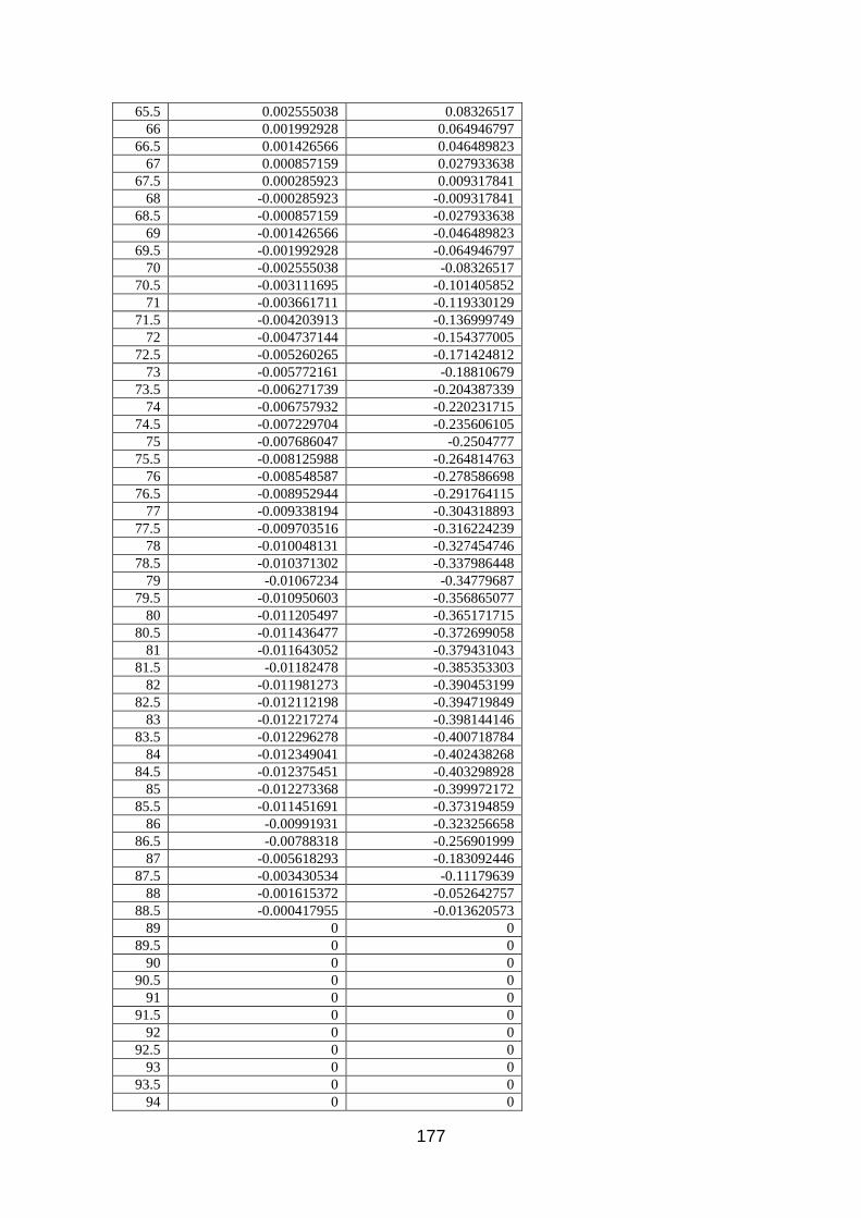
177

65.5 0.002555038 0.08326517

66 0.001992928 0.064946797

66.5 0.001426566 0.046489823

67 0.000857159 0.027933638

67.5 0.000285923 0.009317841

68 -0.000285923 -0.009317841

68.5 -0.000857159 -0.027933638

69 -0.001426566 -0.046489823

69.5 -0.001992928 -0.064946797

70 -0.002555038 -0.08326517

70.5 -0.003111695 -0.101405852

71 -0.003661711 -0.119330129

71.5 -0.004203913 -0.136999749

72 -0.004737144 -0.154377005

72.5 -0.005260265 -0.171424812

73 -0.005772161 -0.18810679

73.5 -0.006271739 -0.204387339

74 -0.006757932 -0.220231715

74.5 -0.007229704 -0.235606105

75 -0.007686047 -0.2504777

75.5 -0.008125988 -0.264814763

76 -0.008548587 -0.278586698

76.5 -0.008952944 -0.291764115

77 -0.009338194 -0.304318893

77.5 -0.009703516 -0.316224239

78 -0.010048131 -0.327454746

78.5 -0.010371302 -0.337986448

79 -0.01067234 -0.34779687

79.5 -0.010950603 -0.356865077

80 -0.011205497 -0.365171715

80.5 -0.011436477 -0.372699058

81 -0.011643052 -0.379431043

81.5 -0.01182478 -0.385353303

82 -0.011981273 -0.390453199

82.5 -0.012112198 -0.394719849

83 -0.012217274 -0.398144146

83.5 -0.012296278 -0.400718784

84 -0.012349041 -0.402438268

84.5 -0.012375451 -0.403298928

85 -0.012273368 -0.399972172

85.5 -0.011451691 -0.373194859

86 -0.00991931 -0.323256658

86.5 -0.00788318 -0.256901999

87 -0.005618293 -0.183092446

87.5 -0.003430534 -0.11179639

88 -0.001615372 -0.052642757

88.5 -0.000417955 -0.013620573

89 0 0

89.5 0 0

90 0 0

90.5 0 0

91 0 0

91.5 0 0

92 0 0

92.5 0 0

93 0 0

93.5 0 0

94 0 0

178

94.5 0 0

95 0 0

95.5 0 0

96 0 0

96.5 0 0

97 0 0

97.5 0 0

98 0 0

98.5 0 0

99 0 0

99.5 0 0

100 0 0

Appendix 5 Tables of the front and rear suspension hard points

Table 0-1 Front suspension hard points

Table 0-2 Rear suspension hard points

179

Appendix 5 Measurement outputs from the front and rear suspension system

All Figures show the outputs for the front suspension characteristics based on the

quarter car model that has been built in the previous section.

Figure 1 Half Track Change Vs Bump Movement (Front)

180

Figure 2 Wheel Recession Vs Bump Movement (Front)

Figure 3 Steering Axis Inclination Vs Bump Movement (Front)

Figure 4 Ground Level Offset Vs Bump Movement (Front)

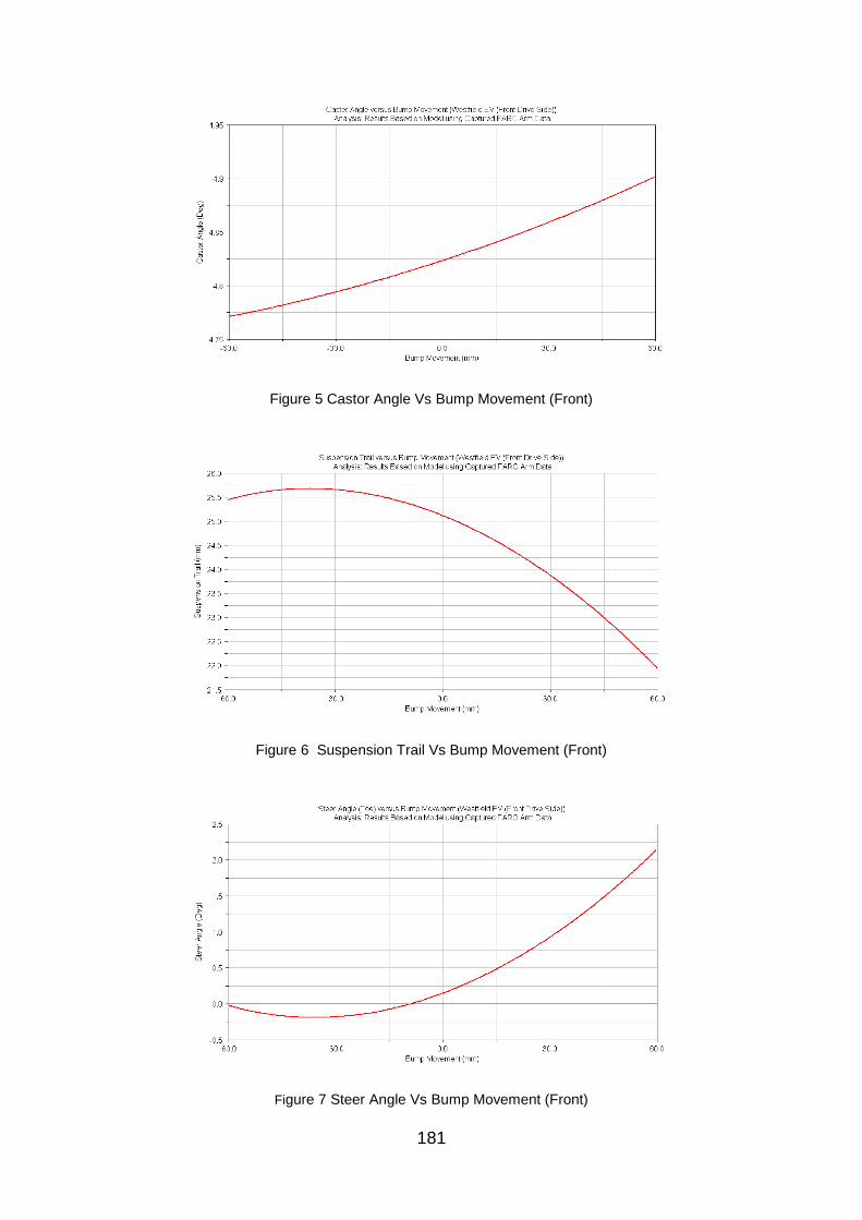
181

Figure 5 Castor Angle Vs Bump Movement (Front)

Figure 6 Suspension Trail Vs Bump Movement (Front)

Figure 7 Steer Angle Vs Bump Movement (Front)

182

Figures show the outputs for the rear suspension characteristics based on the

quarter car model that has been built in the previous section.

Figure 9 Half Track Change Vs Bump Movement (Rear)

Figure 10 Wheel Recession Vs Bump Movement (Rear)

183

Figure 11 Steer Axis Inclination Vs Bump Movement (Rear)

Figure 12 Ground Level Offset Vs Bump Movement (Rear)

Figure 13 Castor Angle Vs Bump Movement (Rear)

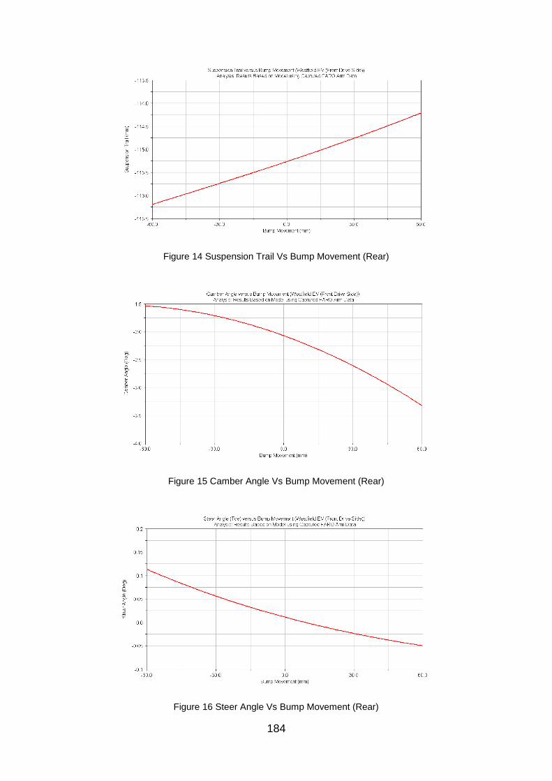
184

Figure 14 Suspension Trail Vs Bump Movement (Rear)

Figure 15 Camber Angle Vs Bump Movement (Rear)

Figure 16 Steer Angle Vs Bump Movement (Rear)