Embed Size (px)
Citation preview

1
Design and Modeling of Slender and Deep beams with Linear Finite Element Method
Master Thesis
March 2014
By Babak Dadvar

2

3
Members of the thesis committee Prof.dr.ir. D.A. Hordijk Delft University of Technology, Faculty of Civil Engineering and Geosciences Section concrete structures
Dr.ir.drs. C.R. Braam Delft University of Technology, Faculty of Civil Engineering and Geosciences Section concrete structures
Dr.ir. P.C.J. Hoogenboom Delft University of Technology, Faculty of Civil Engineering and Geosciences Section structural mechanics
Ir. F.H. Middelkoop Royal HaskoningDHV Section BLDS-SD&ABB - structural design

4

5
Acknowledgement
I would like to thank my Company Supervisor ir. F.H. Middelkoop for his guidance and support during my time at Royal HaskoningDHV. I would also like to express my deep gratitude to my direct thesis supervisor dr.ir.drs. C.R. Braam for his patience and valuable inputs during my thesis course. I am also grateful to my supervisors, prof.dr.ir. D.A. Hordijk and dr. ir. P.C.J. Hoogenboom for their guidance and for sharing their knowledge. I would like to thank ir. Y. Yang and my dear friend A. Rezaeifar for their invaluable assistance.
Finally I would like to thank my parents, who are my role models and who supported me throughout my life in Iran and in the Netherlands. Last but not least, I am also grateful to my sister and my brother for their unconditional support.
Babak Dadvar March 2014 Delft, The Netherlands

6
7
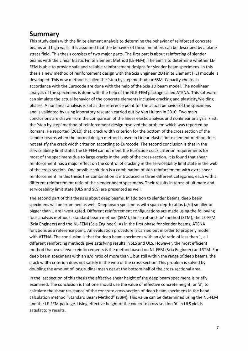
Summary This study deals with the finite element analysis to determine the behavior of reinforced concrete beams and high walls. It is assumed that the behavior of these members can be described by a plane stress field. This thesis consists of two major parts. The first part is about reinforcing of slender beams with the Linear Elastic Finite Element Method (LE-FEM). The aim is to determine whether LE-FEM is able to provide safe and reliable reinforcement designs for slender beam specimens. In this thesis a new method of reinforcement design with the Scia Engineer 2D Finite Element (FE) module is developed. This new method is called the ‘step by step method’ or SSM. Capacity checks in accordance with the Eurocode are done with the help of the Scia 1D beam model. The nonlinear analysis of the specimens is done with the help of the NLE-FEM package called ATENA. This software can simulate the actual behavior of the concrete elements inclusive cracking and plasticity/yielding phases. A nonlinear analysis is set as the reference point for the actual behavior of the specimens and is validated by using laboratory research carried out by Van Hulten in 2010. Two main conclusions are drawn from the comparison of the linear elastic analysis and nonlinear analysis. First, the ‘step by step’ method of reinforcement design resolved the problem which was reported by Romans. He reported (2010) that, crack width criterion for the bottom of the cross section of the slender beams when the normal design method is used in Linear elastic finite element method does not satisfy the crack width criterion according to Eurocode. The second conclusion is that in the serviceability limit state, the LE-FEM cannot meet the Eurocode crack criterion requirements for most of the specimens due to large cracks in the web of the cross-section. It is found that shear reinforcement has a major effect on the control of cracking in the serviceability limit state in the web of the cross section. One possible solution is a combination of skin reinforcement with extra shear reinforcement. In this thesis this combination is introduced in three different categories, each with a different reinforcement ratio of the slender beam specimens. Their results in terms of ultimate and serviceability limit state (ULS and SLS) are presented as well.
The second part of this thesis is about deep beams. In addition to slender beams, deep beam specimens will be examined as well. Deep beam specimens with span-depth ratios (a/d) smaller or bigger than 1 are investigated. Different reinforcement configurations are made using the following four analysis methods: standard beam method (SBM), the ‘strut-and-tie’ method (STM), the LE-FEM (Scia Engineer) and the NL-FEM (Scia Engineer). As in the first phase for slender beams, ATENA functions as a reference point. An evaluation procedure is carried out in order to properly model with ATENA. The conclusion is that for deep beam specimens with an a/d ratio of less than 1, all different reinforcing methods give satisfying results in SLS and ULS. However, the most efficient method that uses fewer reinforcements is the method based on NL-FEM (Scia Engineer) and STM. For deep beam specimens with an a/d ratio of more than 1 but still within the range of deep beams, the crack width criterion does not satisfy in the web of the cross-section. This problem is solved by doubling the amount of longitudinal mesh net at the bottom half of the cross-sectional area.
In the last section of this thesis the effective shear height of the deep beam specimens is briefly examined. The conclusion is that one should use the value of effective concrete height, or ‘d’, to calculate the shear resistance of the concrete cross-section of deep beam specimens in the hand calculation method “Standard Beam Method” (SBM). This value can be determined using the NL-FEM and the LE-FEM package. Using effective height of the concrete cross-section ‘d’ in ULS yields satisfactory results.

8
9
Table of Contents Design and Modeling of Slender and Deep beams with Linear Finite Element Methods ...................... 1
Members of the thesis committee ...................................................................................................... 3
Acknowledgement ............................................................................................................................... 5
Summary ............................................................................................................................................. 7
Chapter 1 Introduction, Literature and scope ....................................................................................... 13
1.1 Introduction ............................................................................................................................. 13
1.2 Literature Review .................................................................................................................... 14
1.3 Objectives and Scope .............................................................................................................. 24
1.4 Thesis Outline .......................................................................................................................... 25
References ..................................................................................................................................... 26
Chapter 2 The LE-FEM and the NL-FEM (Theory) .................................................................................. 28
2.1 Summary .................................................................................................................................. 28
2.2 Normal Slender Beams ............................................................................................................ 28
2.3 Reminder about Plates ............................................................................................................ 31
2.4 Geometrical Imperfections ...................................................................................................... 32
2.5 Non Linear Finite Element Analysis (NL-FEM Theory) ............................................................. 32
2.6 Deep Beams or Walls ............................................................................................................... 35
References ..................................................................................................................................... 44
Chapter 3 Linear Elastic and Nonlinear Finite Element Method (specifications) .................................. 46
3.1 Summary .................................................................................................................................. 46
3.2 Slender and Deep Beams ......................................................................................................... 46
References ..................................................................................................................................... 58
Chapter 4 Reinforcing the Specimens (LE-FEM & NL-FEM) ................................................................... 59
4.1 Summary .................................................................................................................................. 59
4.2 Introduction ............................................................................................................................. 59
4.3 Design of Reinforcements for Slender and Deep BEAMS in LE-FEM ....................................... 59
4.4 Process of Reinforcing ............................................................................................................. 61
4.5 Design of Reinforcements in Deep Beams in NL-FEM ............................................................. 64
References ..................................................................................................................................... 65
Chapter 5 Required Verifications in Limit States................................................................................... 66
5.1 Summary .................................................................................................................................. 66
5.2 Slender Beams ......................................................................................................................... 66
References ..................................................................................................................................... 86
10
Chapter 6 Non-Linear Finite Element Analysis: Principles, Slender and Deep beams .......................... 87
6.1 Summary .................................................................................................................................. 87
6.2 Introduction ............................................................................................................................. 87
6.3 Model Parameters and Specifications in Nonlinear Finite Element Analysis .......................... 87
6.4 Summary of Material Properties in ATENA ............................................................................. 98
6.5 Recommendations ................................................................................................................. 100
References ................................................................................................................................... 100
Chapter 7 ATENA vs Laboratory Test .................................................................................................. 102
7.1 Summary ................................................................................................................................ 102
7. 2 Introduction .......................................................................................................................... 102
7.3 ATENA vs Laboratory Test ..................................................................................................... 102
7.4 Behavior during Laboratory Test ........................................................................................... 103
7.5 Validation Process ................................................................................................................. 104
7.6 Results ................................................................................................................................... 107
7.7 Conclusion ............................................................................................................................. 107
7.8 Recommendations ................................................................................................................. 108
References ................................................................................................................................... 108
Chapter 8 ATENA vs SCIA: Analysis and Interpretation of the Results ................................................ 109
8.1 Summary ................................................................................................................................ 109
8.2 Introduction ........................................................................................................................... 109
8.3 Summary of the SBETA Material Model in ATENA ................................................................ 109
8.4 Serviceability Limit State (SLS) ............................................................................................... 110
8.5 Recommendations SLS .......................................................................................................... 116
8.6 Ultimate Limit State (ULS) ..................................................................................................... 116
8.7 Observations and Conclusions in ULS Only ........................................................................... 118
8.8 Conclusions ULS and SLS and Recommendations ................................................................. 119
8.9 Recommendations ................................................................................................................. 121
References ................................................................................................................................... 122
Chapter 9 ATENA Evaluation for Deep Beam Specimens-Analysis and Interpretation of the Results 123
9.1 Summary ................................................................................................................................ 123
9.2 Introduction ........................................................................................................................... 123
9.3 Summary of the Deep Beam Specimens ............................................................................... 123
9.4 Geometry of the Specimen D1 .............................................................................................. 123
9.5 Adjustment Procedure .......................................................................................................... 123

11
9.6 Conclusion ............................................................................................................................. 127
References ................................................................................................................................... 127
Chapter 10 Comparing SBM, STM, LE-FEM and NL-FEM Reinforcing Methods by Using ATENA for DEEP Beam Specimens ........................................................................................................................ 128
10.1 Summary .............................................................................................................................. 128
10.2 Introduction ......................................................................................................................... 128
10.3 Table of the Deep Beam Specimens .................................................................................... 128
10.4 Table of Deep Beam Specimens Based on Reinforcement Configurations ......................... 129
10.5 Serviceability Limit State (SLS) ............................................................................................. 129
10.6 Ultimate Limit State (ULS) ................................................................................................... 132
10.7 Shear Effective Height ......................................................................................................... 138
10.8 Guideline to Limit Crack Width of D2 (1<a/d<2) Deep Beam Specimens ........................... 141
10.9 Recommendations ............................................................................................................... 141
References ................................................................................................................................... 142
Chapter 11 Conclusions and recommendations ................................................................................. 143
11.1 introduction ......................................................................................................................... 143
11.2 Conclusions for Slender beams ........................................................................................... 143
11.3 Conclusions for Deep beams ............................................................................................... 145
11.4 Recommendations ............................................................................................................... 146

12
13
Chapter 1 Introduction, Literature and scope
1.1 Introduction One of the most important building materials is reinforced concrete (RC). It is widely used in many types of engineering structures. Its low price, efficiency, strength and stiffness make it an attractive material for a wide range of structural applications. Generally, concrete as a building material must satisfy the following conditions:
(1) The structure must be strong and safe. The proper application of the fundamental principles of analysis, the laws of equilibrium and the consideration of the mechanical properties of the component materials should demonstrate that the structure can take accidental overloads without collapsing.
(2) The structure must be stiff. Care must be taken to control deflections under service loads and to limit the crack width to an acceptable level.
(3) The structure must be economical. Materials must be used efficiently, since the difference in unit cost between concrete and steel is relatively large.
There is a constant need for experimental research to develop advanced design and analysis methods for modern structures.
Laboratory tests supply basic information for finite element models, such as material properties. In addition, the results of finite element models have to be evaluated by comparing them with experiments on full-scale models of structural elements or even entire structures. Given the fact that tests are time-consuming and costly and often fail to exactly simulate the loading and support conditions of the actual structure, developing reliable analytical models can reduce the number of test specimens required for the solution of a given problem.
The development of analytical models of the response of RC structures is complicated by the following three factors:
• Reinforced concrete is a composite material made up of concrete and steel, two materials that display very different physical and mechanical behavior.
• Concrete exhibits nonlinear behavior even under low level loading, environmental effects, cracking, biaxial stiffening and strain softening.
• Reinforcing steel and concrete interact in a complex way through bond-slip. Cracked concrete behavior is influenced by aggregate interlock.
These complex phenomena have led engineers to rely heavily on empirical formulas for the design of concrete structures, which were derived from numerous experiments. Advanced digital computers and powerful methods of analysis, such as the finite element method, however, have reduced the need for costly and time-consuming experiments.
Numerical calculations based on the finite element method are becoming a normal standard tool in design of structures. Linear and nonlinear finite element software packages (respectively the LE-FEM

14
and the NLE-FEM) are becoming more user-friendly and computers are becoming faster every day. These improvements have considerable potential for the numerical calculation based on finite element methods. However, doing nonlinear finite element analysis is still is a complex and time-consuming process, which means that in engineering practices it can be used only rarely. At the same time, though, software packages like Scia Engineer, which is able to do fast linear and nonlinear calculations, give ground for optimism. This kind of user-friendly software has become more and more popular in the reinforcement design of different reinforced concrete elements. Nevertheless, it remains to be seen whether a LE-FEM package can be a good replacement for NL-FEM package.
The present study is part of this continuing effort. It presents an analysis of reinforced concrete slender and deep beams with the help of Scia Engineer and a comparison of the results of nonlinear software packages like ATENA.
1.2 Literature Review In this section a brief review of previous studies about the application of the finite element method for the linear and nonlinear analysis of reinforced concrete structures is presented.
1.2.1 Romans (2010) In his thesis on the design of walls with LE-FEM, Romans [1] mentioned two possible ways in which the LE-FEM deviates from common design methods, such as the strut-and-tie method, in the reinforcement design process and the underlying principles.
Deviation 1 Common design assumes that concrete is only capable of transferring compressive forces. The strut-and-tie method (a possible approach of the actual behavior) takes into account load transfer mechanisms that correspond with the typical strength properties of the applied materials (figure 1.1).
Figure 1.1: load transfer mechanisms according to the STM [1]
LE-FEM assumes isotropic, un-cracked linear elastic isotropic behavior.

15
Figure 1.2 Stress trajectories that follow from a LE-FEM [1]
The question is whether the applied orthogonal reinforcement that is derived directly from the membrane forces (figure 1.2) will transfer loads in a similar way as is assumed in the LE-FEM.
Deviation 2 In LE-FEM the moment diagram is not shifted over a specific distance. Codes like NEN-EN 1992-1-1 [1] and NEN6720 [2] prescribe a shift in the moment line to calculate the actual longitudinal steel stresses from a vertical cross-sectional analysis.
Figure 1.3 Shifting of the moment line, NEN6720[1]
This being the case, the limited reinforcement, which according to the LE-FEM is required at supports, can cause problems.
Romans tried to find out to what extent these deviations have an influence on the structural behavior or the resistance to failure of reinforced concrete deep beams or walls. His conclusions include the following [1]:
• Regarding possible deviation 1, he found that linear elastic material behavior of concrete in LE-FEM does not approach concrete behavior in an accurate way. This approach results in the development of load transfer mechanisms that deviate from the mechanisms that are expected to develop in practice (figure 1.4 left). The development of a tension arch to transfer loads to supports as was observed in the LE-FEM, is not observed again in the NL-FEM. NL-FEM takes the effect of stress redistribution due to cracking into account. As a result, the NL-FEM’s load transfer mechanism deviates from that of the LE-FEM. To equilibrate the horizontal component of the strut forces, the longitudinal reinforcement in the tension zone has to transfer higher loads than initially assumed in the design process based on linear elastic analysis. This results in a considerable cracks and relatively high compressive forces in the compressive zone.
16
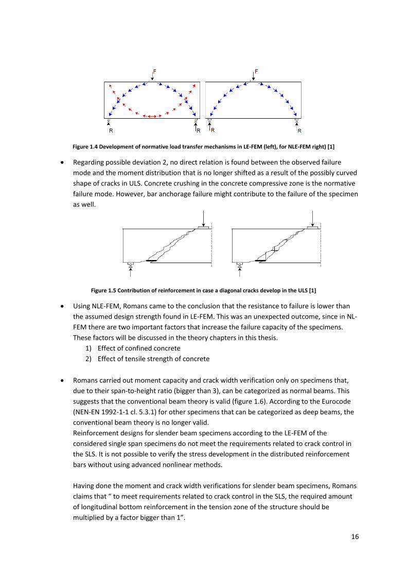
Figure 1.4 Development of normative load transfer mechanisms in LE-FEM (left), for NLE-FEM right) [1]
• Regarding possible deviation 2, no direct relation is found between the observed failure mode and the moment distribution that is no longer shifted as a result of the possibly curved shape of cracks in ULS. Concrete crushing in the concrete compressive zone is the normative failure mode. However, bar anchorage failure might contribute to the failure of the specimen as well.
Figure 1.5 Contribution of reinforcement in case a diagonal cracks develop in the ULS [1]
• Using NLE-FEM, Romans came to the conclusion that the resistance to failure is lower than the assumed design strength found in LE-FEM. This was an unexpected outcome, since in NL-FEM there are two important factors that increase the failure capacity of the specimens. These factors will be discussed in the theory chapters in this thesis.
1) Effect of confined concrete 2) Effect of tensile strength of concrete
• Romans carried out moment capacity and crack width verification only on specimens that,
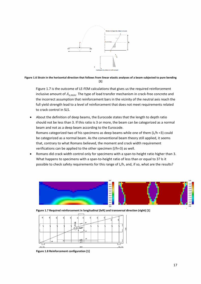
due to their span-to-height ratio (bigger than 3), can be categorized as normal beams. This suggests that the conventional beam theory is valid (figure 1.6). According to the Eurocode (NEN-EN 1992-1-1 cl. 5.3.1) for other specimens that can be categorized as deep beams, the conventional beam theory is no longer valid. Reinforcement designs for slender beam specimens according to the LE-FEM of the considered single span specimens do not meet the requirements related to crack control in the SLS. It is not possible to verify the stress development in the distributed reinforcement bars without using advanced nonlinear methods. Having done the moment and crack width verifications for slender beam specimens, Romans claims that “ to meet requirements related to crack control in the SLS, the required amount of longitudinal bottom reinforcement in the tension zone of the structure should be multiplied by a factor bigger than 1”.
17
Figure 1.6 Strain in the horizontal direction that follows from linear elastic analyses of a beam subjected to pure bending [1]
Figure 1.7 is the outcome of LE-FEM calculations that gives us the required reinforcement inclusive amount of 𝐴𝑠,𝑚𝑖𝑛. The type of load transfer mechanism in crack-free concrete and the incorrect assumption that reinforcement bars in the vicinity of the neutral axis reach the full yield strength lead to a level of reinforcement that does not meet requirements related to crack control in SLS.
• About the definition of deep beams, the Eurocode states that the length to depth ratio should not be less than 3. If this ratio is 3 or more, the beam can be categorized as a normal beam and not as a deep beam according to the Eurocode. Romans categorized two of his specimens as deep beams while one of them (L/h =3) could be categorized as a normal beam. As the conventional beam theory still applied, it seems that, contrary to what Romans believed, the moment and crack width requirement verifications can be applied to the other specimen (l/h=3) as well.
• Romans did crack width control only for specimens with a span-to-height ratio higher than 3. What happens to specimens with a span-to-height ratio of less than or equal to 3? Is it possible to check safety requirements for this range of L/h, and, if so, what are the results?
Figure 1.7 Required reinforcement in longitudinal (left) and transversal direction (right) [1]
Figure 1.8 Reinforcement configuration [1]

18
1.2.2 Mahmoud (2007) Mahmoud [2] also researched design and numerical analyses of reinforced concrete deep beams. He used two common design methods, i.e. the strut-and-tie method (STM) and the Beam method, to calculate the internal forces and to design deep beams. In addition, he also used the LE-FEM and NLE-FEM. The goal was to find the most economical way to design deep beams. It was concluded that the best deep beam design method is LE-FEM because it is fast and the results satisfy all design requirements.1
Problems, conclusions and recommendations for further study
• Mahmoud used LE-FEM package that was in fact an old version of Scia Engineer. The record regarding the use of Scia Engineer shows that newer versions may give other results than older ones. The developers of Scia Engineer are always updating the program modules, use newer methods for each version and incorporate new versions of the Eurocode or other international codes in the program. This is also why the results from the old version of Scia Engineer, which was also a student version, were not reliable anymore.
Figure 1.9 Figures shown additional horizontal (left) and vertical (right) reinforcement needed according to SCIA.ESA PT version 7.0.161 [2]
• The SLS crack width check in the LE-FEM was done using the Eurocode (NEN-EN 1992-1-1 cl. 7.3), which is based on tensile stresses in the bottom reinforcements. The crack width results from the LE-FEM at the bottom fiber of the beams were interpreted in different way than the results from the NL-FEM.
• As results of the previous point, the use of the LE-FEM and the NLE-FEM can lead to different results regarding the best design method to design deep beams.
• Mahmoud discussed the method of reinforcing for deep beams, as well as the type of finite elements to be used for modeling in Scia ESA PT. These methods and options in Scia ESA PT can be optimized in the newer versions of Scia Engineer.
1 The LE-FEM Mahmoud used, was an earlier version of Scia Engineer called ESA-PT, which was self a newer version of ESA Prima WIN. The version used in his thesis was SCIA ESA PT version 7.0.161 (student version). For nonlinear analysis an unknown version of ATENA was used.

19
• Some controls were done partly by hand calculations due to the limited capability of the old version of Scia Engineer software (SCIA.ESA PT version 7.0.161). This might be not the case anymore, since this issue may have been addressed in the full version of Scia Engineer 2011, which is used in this thesis.
Figure 1.10 Two examples of failure of specimens in ATENA software [2]
• The non-linear analyses of these deep beams reveal that the designs from the three calculation methods gave sufficient load carrying capacity for the ULS. However for some designs the capacity was much larger than needed. The principle of using nonlinear finite element method software (ATENA) will be use also in this thesis.
Some absent (in 2007 not yet) included features in SCIA.ESA PT version 7.0.161 (student version)
• The student version of SCIA.ESA PT was not able to model plates and lines and 1D and 2D elements, nor could it connect them in 3D structures.
• Adding extra reinforcement bars by the opening in a plate was not possible. • Manual user interface options were limited. • Crack width control could not be used because there was no option to add additional bars to
the mesh reinforcements. • Many of the program’s results were unclear to the user.
1.2.3 Asin (1999) Asin [3] mentions some possible deviations in behavior between deep beams and slender beams:
• Because of the characteristically small ratio between shear span and depth, deep beams behave differently from slender beams.
• The response of deep beams is characterized by a nonlinear strain distribution and a significant direct load transfer from the point of loading to the supports.
• Deep beams are generally very stiff, which makes them sensitive to imposed deformations such as differential support settlements.
• As the shear deformation, unlike bending moment deformation, is not negligible, the conventional beam theory is not able to predict the load distribution within continuous deep beams.

20
Starting out from of these differences and at a time when the structural behavior of continuous deep beams was not yet completely understood, Asin has carried out an experimental and numerical research project. He specifically studied the contribution of and the interaction between the different load bearing mechanisms and developed a model that describes the observed behavior. The aim of this research project was to study the structural behavior of reinforced concrete continuous deep beams as influenced by the ratio of top and bottom reinforcement, the level of shear reinforcement, and the slenderness. Asin’s research could be divided into five important parts:
1. Review of earlier published work 2. Experimental research 3. In chapter 3 he gave a description of load bearing mechanisms in continuous deep beams. He
then went on to describe the specimens in terms of geometry, reinforcement and boundary conditions. Then he reported on the loading scheme and the arrangement of measuring devices. The experimental program consisted of 14 large scale continuous deep beams with different levels of the slenderness, different top and bottom reinforcement ratios, and different levels of vertical web reinforcement.
Figure 1.11 Load bearing mechanisms [3]
4. Numerical simulations In chapter 5 Asin focused on nonlinear finite element analysis. Finite modeling of a deep beam, constitutive relations and comparison of simulations with an experiment is reviewed. In the last part the prediction of the structural behavior of the tested continuous deep beam by using the program SBETA is discussed.
5. The development of a description model. In chapter 6 he develops a description model based on the observed behavior. The model’s basic component is a strut-and-tie model.

21
Conclusions with regard to overall structural response (after the test)
• The crack pattern development suggests that the behavior of continuous deep beams is fundamentally different from that of slender beams.
• The load-deflection response is very stiff and depends on the slenderness. The ratio between top and bottom reinforcement does not have a pronounced influence. The level of shear reinforcement largely determines the ultimate load.
• With increased slenderness the strut-and-tie action decreased. • The best results are reportedly generated by smeared crack models in which perfect bond is
assumed. • Correct modeling of shear transfer in cracked concrete, and the modeling of compressive
softening are important to adequately predict the correct failure mode. • Quite some agreement was found between the experiment and the simulation over the
whole experimental range. This went for both overall and for local behavior, which suggests that nonlinear analysis adequately predicts the behavior of continuous deep beams.
1.2.4 Van Hulten (2011) Van Hulten’s [4] work is something of a sequel to the earlier work of Romans [1]. Van Hulten began his work by noting that in Romans’ report stated that the load bearing capacity as determined by the LE-FEM did not match with the maximum acting load that was found in the NLE-FEM package. The capacity according to NLE-FEM is lower than the load capacity according to LE-FEM. In order to come to a full understanding of this discrepancy, Van Hulten carried out an experiment in the Stevin laboratory. He started out from the possibility that an LE-FEM software package could be useful in designing a concrete deep beam. His research question was whether this is indeed the case and whether this way of working yields results that meet the safety requirements? His sub-questions were the following:
• What is the actual bearing capacity according to the Diana finite element model? • Do the results from DIANA (another nonlinear finite element program) differ substantially
from those of ATENA? • How can we interpret the test result for further research? • Which stress relation is the most accurate reflection of reality?
The steps he has followed in his research can be summarized as following:
• Literature study • Experiment in Stevin Laboratory. Romans’ specimen S-2-4 from Romans is 3 meters long, 1
meter high and 0.2 meters thick (figure 1.12). It has no reinforcement mesh and is designed as much as possible in accordance with the LE-FEM results.
• Calculation with DIANA and comparison of the experiment results. Different combinations have been examined with the DIANA input.
• Different reinforcement configurations • Evaluation of the results

22
Figure 1.12 Reinforcement drawing of specimen S-2-4
Related results, conclusions and recommendations
The ultimate load according to DIANA is lower than the design load according to LE-FEM. (This confirms Romans’ conclusion that the assumed design strength (LE-FEM) is higher than the resistance to failure results of NLE-FEM.)
• Shortening or extension of the reinforcement mesh has a strong influence on the bearing capacity.
• The “smeared cracking model” that was used, gives a very widespread pattern of cracks. • The results of the FEM models give a lower capacity than the design load. However, the
analysis in the DIANA model and test results correspond very closely. Thus, the DIANA model yielded good results and can be used for further research. The lower bearing capacity according to the FEM models are in accordance with the possible overestimation of the nominal load.
• An appropriate bond-slip model is desirable.
1.2.5 Kwak and Filippou Kwak and Filippou [5] wrote about finite element analysis of the monotonic behavior of reinforced concrete beams, slabs and beam column joint sub-assemblages. An assumption was made to allow the description of the behavior of these members by a plane stress field. Concrete and reinforcing steel were represented by separate material models that were combined with a model of the interaction between reinforcing steel and concrete through bond-slip. Together, these models describe the behavior by two failures in the biaxial stress space and one failure surface in the biaxial strain space.
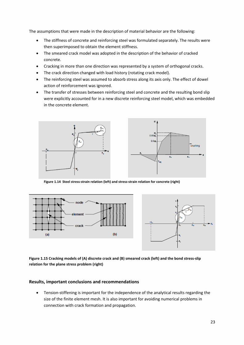
Concrete was assumed as linear elastic material for the stress states inside the initial yield surface. For stresses outside this surface the behavior of concrete was described by a nonlinear orthotropic model, whose orthotropic axes paralleled the principal strain directions.
The behavior of cracked concrete was described by a system of orthogonal cracks, which follow the principal strain directions and were thus rotating during the load history.
Comparisons of analytical and experimental results were conducted to establish the validity of the proposed models and to determine the importance of various effects on the local and global response of reinforced concrete (RC) members.
23
The assumptions that were made in the description of material behavior are the following:
• The stiffness of concrete and reinforcing steel was formulated separately. The results were then superimposed to obtain the element stiffness.
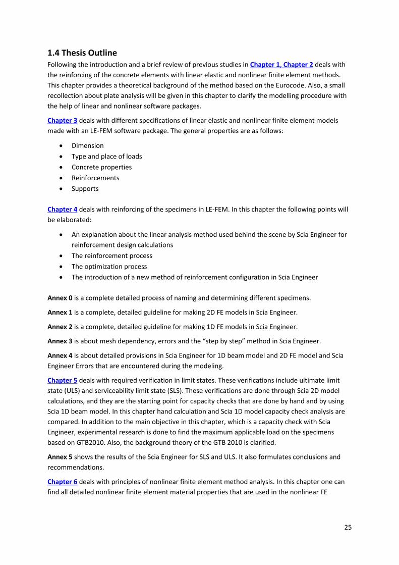
• The smeared crack model was adopted in the description of the behavior of cracked concrete.
• Cracking in more than one direction was represented by a system of orthogonal cracks. • The crack direction changed with load history (rotating crack model). • The reinforcing steel was assumed to absorb stress along its axis only. The effect of dowel
action of reinforcement was ignored. • The transfer of stresses between reinforcing steel and concrete and the resulting bond slip
were explicitly accounted for in a new discrete reinforcing steel model, which was embedded in the concrete element.
Figure 1.14 Steel stress-strain relation (left) and stress-strain relation for concrete (right)
Figure 1.15 Cracking models of (A) discrete crack and (B) smeared crack (left) and the bond stress-slip relation for the plane stress problem (right)
Results, important conclusions and recommendations
• Tension-stiffening is important for the independence of the analytical results regarding the size of the finite element mesh. It is also important for avoiding numerical problems in connection with crack formation and propagation.

24
• Tension-stiffening and bond-slip have opposite effects on the response of RC members. Tension-stiffening accounts for the concrete tensile stresses between cracks, and it increases the stiffness of the member. Bond-slip causes reduction in stiffness. In lightly reinforced beams, these two effects can compensate each other at certain load stages. This may give the false impression that they can be neglected in the analysis. Bond-slip increases with loading, while tension-stiffening does not. For the sake of consistency, reliable results can only be obtained when both effects are included in the model. It is important to know that the effect of bond-slip clearly outweighs the contribution of tension stiffening in heavily reinforced beams. In these cases ignoring the bond-slip effect can cause a major over-estimation of the stiffness of the member.
• Present smeared models are too stiff in connection with large finite elements. A new criterion that limits the effect of tension stiffening to the vicinity of the integration point yields very satisfactory results.
• The tensile strength of concrete has no significant effect on the load-displacement response of reinforced concrete (RC) beams (SLS). Fracture energy is the most important factor that influences crack formation and propagation.
1.2.6 Other related literatures “The earliest publication on the application of the finite element method to the analysis of RC structures was presented by Ngo and Scordelis [6]. In their study, simple beams were analyzed with a model in which concrete and reinforcing steel were represented by constant strain triangular elements, and a special bond link element was used to connect the steel to the concrete and describe the bond-slip effect. A linear elastic analysis was carried out on beams with predefined crack patterns to determine principal stresses in concrete, stresses in steel reinforcement and bond stresses. Since the publication of this pioneering work, the analysis of reinforced concrete structures has enjoyed a growing interest and many publications have appeared.”
1.3 Objectives and Scope The present research is an analysis using the finite element method of the reinforcement design process of beams in the first phase and deep beams in the second phase.2 This thesis builds on the research results and recommendations from other researchers and is limited to structural elements that frequently occur in practice. Slender and deep beams loaded in their plane (membrane state) are two such structural elements.
The main objectives of this study are:
• To improve the reinforcement design method in the LE-FEM, for slender and deep beams. • To investigate whether the results from LE-FEM are comparable to the actual behavior. • To investigate the possible use of nonlinear finite element analysis with Scia Engineer. • To investigate and compare different design methods for analyzing of deep beam specimens.
2 The LE-FEM and NL-FEM analysis with specific module which is implemented into Scia Engineer are used for the design method.
25
1.4 Thesis Outline Following the introduction and a brief review of previous studies in Chapter 1, Chapter 2 deals with the reinforcing of the concrete elements with linear elastic and nonlinear finite element methods. This chapter provides a theoretical background of the method based on the Eurocode. Also, a small recollection about plate analysis will be given in this chapter to clarify the modelling procedure with the help of linear and nonlinear software packages.
Chapter 3 deals with different specifications of linear elastic and nonlinear finite element models made with an LE-FEM software package. The general properties are as follows:
• Dimension • Type and place of loads • Concrete properties • Reinforcements • Supports
Chapter 4 deals with reinforcing of the specimens in LE-FEM. In this chapter the following points will be elaborated:
• An explanation about the linear analysis method used behind the scene by Scia Engineer for reinforcement design calculations
• The reinforcement process • The optimization process • The introduction of a new method of reinforcement configuration in Scia Engineer
Annex 0 is a complete detailed process of naming and determining different specimens.
Annex 1 is a complete, detailed guideline for making 2D FE models in Scia Engineer.
Annex 2 is a complete, detailed guideline for making 1D FE models in Scia Engineer.
Annex 3 is about mesh dependency, errors and the “step by step” method in Scia Engineer.
Annex 4 is about detailed provisions in Scia Engineer for 1D beam model and 2D FE model and Scia Engineer Errors that are encountered during the modeling.
Chapter 5 deals with required verification in limit states. These verifications include ultimate limit state (ULS) and serviceability limit state (SLS). These verifications are done through Scia 2D model calculations, and they are the starting point for capacity checks that are done by hand and by using Scia 1D beam model. In this chapter hand calculation and Scia 1D model capacity check analysis are compared. In addition to the main objective in this chapter, which is a capacity check with Scia Engineer, experimental research is done to find the maximum applicable load on the specimens based on GTB2010. Also, the background theory of the GTB 2010 is clarified.
Annex 5 shows the results of the Scia Engineer for SLS and ULS. It also formulates conclusions and recommendations.
Chapter 6 deals with principles of nonlinear finite element method analysis. In this chapter one can find all detailed nonlinear finite element material properties that are used in the nonlinear FE

26
software package (ATENA). Different options in the program will be briefly described and explained. The following material properties will be discussed:
• Concrete model • Crack models • Steel model • Reinforcement models • Bond model • Interface element
Annex 6 is a guideline for modelling in the nonlinear FE software package ATENA. This chapter is specifically written for this thesis. By following the steps in this chapter, one can reproduce the specimens that are examined in his thesis.
Chapter 7 Deals with the validation procedure of ATENA results. The aim of this chapter is to show that nonlinear analysis results from ATENA analysis are reliable.
Annex 7 gives some example files for ATENA validation process.
Chapter 8 compares between Scia Engineer and ATENA results, which will be interpretation and analyzed. In the final part of this chapter contains conclusions and recommendations that can be drawn from this comparison.
Annex 8 lists all Scia Engineer checks and design calculations.
Chapter 9 is about evaluation of ATENA models for analysis of deep beam specimens.
Annex 9 lists all Maple sheets that are used in this thesis.
Chapter 10 outlines the results of the deep beam analysis and contains a comparison of various reinforcement configuration methods. The behavior of deep beam specimens in SLS and ULS is analyzed. The results are then compared to the ATENA results. Annex 10 gives some Scia Engineer and ATENA models related to deep beams. Chapter 11 gives conclusions and recommendations related to the objectives and scope of this thesis
References [1] Master thesis “Design of walls with linear elastic finite element methods” Marc Romans
2010, TU Delft, concrete structures [2] Master thesis “Design and numerical analysis of the reinforced concrete deep beams” Moufaq Noman Mahmoud (2007), TU Delft, concrete structures [2]

27
[3] PhD thesis “The behavior of reinforced concrete continuous deep beams” Melvin Asin 1999, TU Delft, concrete structures
[4] Master thesis “Loading capacity of reinforced concrete deep beams”, Bart van Hulten (2011), TU Delft, concrete structures [5] Report “Finite element Analysis of reinforced concrete structures under Monotonic Loads” H.G. Kwak and Filip C. Flippou, Civil Engineering, University of California, Nov 1990
[6] Journal of ACI “Finite Element Analysis of Reinforced Concrete Beams” Ngo. D and Scordelis, October 2009 [7] “Challenges and changes in the design of concrete structures” J.G MacGregor 1984
28
Chapter 2 The LE-FEM and the NL-FEM (Theory)
2.1 Summary In this chapter the theory of linear elastic and nonlinear analysis is introduced. This theory is underpins all linear and nonlinear analyses in this thesis. It is also mentioned that all relations are based on Eurocode NEN-EN 1992-1-1. One of the main subjects discussed in this chapter is the subjection of membrane elements to in-plane forces. Another is the Eurocode-based method of reinforcing that will be outlined. In order to deal with the complexity of the different options in the LE-FEM software package, the theory of plates is briefly introduced. In the nonlinear theory part, different nonlinearities are defined. Finally, different analysis methods for deep beam specimens with their global design procedures are introduced.
2.2 Normal Slender Beams
2.2.1 Introduction Simplified methods for determining reinforcement according to NEN-EN 1992-1-1 cl. 5.1.1 (3), enable engineers to determine the required amount of reinforcement from the in-plane stress fields. Since the 1960s authors like Baumann, Braestrup and Nielsen [10] have made a design for reinforced concrete elements subjected to membrane states. This process resulted in formulas for reinforcement design and the checking of concrete strength in the CEB-FIP Code 1990 for concrete structures. The ‘three layer sandwich’ model and the Wood-Armer method [11] were introduced for this purpose. According to NEN-EN-1992-1-1 cl.5.1.1 (3), these models are all possible and acceptable simplified models. For the sake of full compliance to the Eurocode, during this thesis it was tried to make references to the specific Eurocode articles.
2.2.2 Reinforcement design using linear analysis The design of reinforced concrete structures involves the following steps:
1. Select the initial dimensions of all structural elements 2. Execute a global structural analysis to calculate the internal forces 3. Verify concrete initial dimensions and calculate and design the reinforcement capable of
resisting the internal forces.
In this chapter a design method called the ‘three layer sandwich’ model is used for reinforcement design of membrane states. This method is also elaborated in NEN-EN 1992-2 cl. 6.109 [4].
2.2.3 Idealizations According to NEN EN 1992-1-1 cl 5.1.1 (6), common idealizations of the behavior used for analysis are:
• Linear elastic behavior • Linear elastic behavior with limited redistribution • Plastic behavior, including strut-and-tie models (see the sections 2.5 and 2.6) • Nonlinear behavior (see section 2.5)

29
In general, shear walls and deep and normal beams are thin 2D flat spatial structures that are loaded by forces parallel to the mid-plane of the membrane. According to NEN-EN 1992-2-2 cl. 6.109(101), membrane elements may be used for the design of two-dimensional concrete elements subjected to a combination of internal forces. The elements will be evaluated by means of a linear finite element analysis. Membrane elements are subjected only to in-plane forces, namely 𝜎𝐸𝑑𝑥 , 𝜎𝐸𝑑𝑦 and 𝜏𝐸𝑑𝑥𝑦 as shown in Figure 1.1.
Figure 2.1 Membrane element (106 NEN-EN-1992-2-2) [4]
According to NEN-EN 1992-1-1 cl.5.1.1 (4), structural analysis can be done through an idealization of both geometry and the behavior of the structure. Idealizations based on NEN-EN 1992-1-1 cl. 5.1.1(6) can be categorized in four types [3].
• Linear elastic behavior that assumes uncracked cross sections and perfect elasticity. The design procedures for linear analysis are given in NEN-EN 1992-1-1 cl.5.4. This category is going to be used in the “slender beam” section of this thesis.
• Linear elastic behavior with limited redistribution (NEN-EN 1992-1-1 cl.5.5). It is a design procedure (not an analysis) based on mixed assumptions derived from both the linear and the non-linear analysis.
• Plastic behavior. Its kinematic approach (NEN-EN 1992-1-1 cl.5.6) assumes at ultimate limit state the transformation of the structure into a mechanism through the formation of plastic hinges. In its static approach, the structure is made up of compressed and tensioned elements (strut-and-tie model).
• Nonlinear behavior that takes into account cracking, plasticization of reinforcement steel beyond yielding, and plasticization of compressed concrete. The design procedures for non-linear analysis are given in NEN-EN 1992-1-1 cl. 5.7. This category is used by NL-FEM software packages.
Reinforced concrete is a composite, inhomogeneous material that displays very complex nonlinear material behavior. Designing an exact model to simulate the nonlinear behavior of these elements is far too challenging for daily structural design. Therefore, the calculations of the member forces are mostly based on a linear elastic material model.
According to NEN-EN 1992-1-1 2011 cl.5.4, which pertains to the determination of load effects, linear analysis may be used assuming crack-free cross sections, linear stress-strain relationships and the mean value of the modulus of elasticity.

30
According to EN-1992-1-1 cl.5.1.1 (2), local analysis may be used if the assumption of linear strain distribution is not valid, that is, in the vicinity of supports, near concentrated load, in beam-column intersections, in anchorage zones and at changes in cross-sections.
The design of plane shell or membrane elements in the LE-FEM is based on the following assumptions [2].
• Concrete takes no tension. This assumption does not apply to SLS. To get realistic results one has to take into account a reasonable tensile strength of concrete. (NEN-EN 1992-1-1 2011 section 6.1). It is important to mention that initially tension is introduced in the membrane elements, so the assumption of ‘concrete takes no tension’ can be interpreted in different ways.
• Cracks are oriented orthogonally to the principal tensile stress. The location of the cracks depends not only on the location of the stresses but rather on the reinforcement rebar configurations.
• Mohr’s failure criterion is applied. Research is still being done to develop a consistent model to describe the behavior of reinforced concrete member.
• Sufficient ductility. Redistribution of forces after cracking limits the capacity of the reinforced concrete section. Because of this, the assumed load path after cracking should be similar to the elastic flow of forces. A reduction factor about 0.8 should be used to account for concrete’s compressive strength and for the tensile stresses that are lower than the uni-axial compressive strength (EN-1992-1-1 cl. 3.1.6 (1)).
2.2.4 Three layer sandwich model (Eurocode) According to NEN-EN 1992-1-1 cl. 5.1.1 (3), a simplified method for determining reinforcement may be used for in-plane stress fields. Regarding bending (with or without axial force) vis-à-vis the determination of the ultimate moment resistance of reinforced concrete cross-sections, the following assumptions are made [3]:
• Plane sections remain plane. • The strain in bonded reinforcement or bonded pre-stressing tendons, whether in tension or
in compression, is the same as that in the surrounding concrete. • The tensile strength of the concrete is ignored. • The stresses in the concrete in compression are derived from the design stress-strain
relationship given in NEN-EN 1992-1-1 cl. 3.1.7. • The stresses in the reinforcement are derived from the design curves in 3.2 (Figure 3.8) and
3.3 (Figure 3.10) from NEN-EN 1992-1-1. The following expressions from NEN-EN 1992-1-1 Annex F can be used to derive the tension reinforcement in an element subjected to in-plane orthogonal stresses directly from the known membrane force. This method is also explained more elaborately in chapter 16 of the Blaauwendraad’s book [1].
The tensile strength provided by reinforcement should be determined from:
tdx x ydf fρ= tdy y ydf fρ=
31
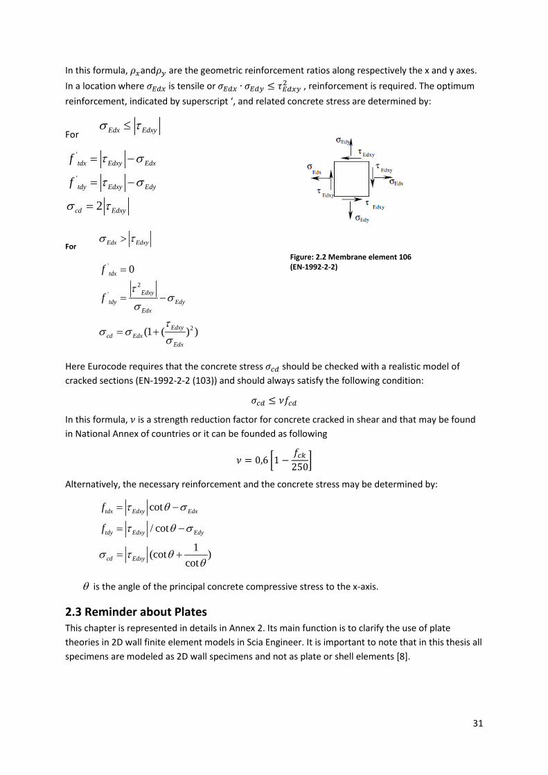
In this formula, 𝜌𝑥and𝜌𝑦 are the geometric reinforcement ratios along respectively the x and y axes. In a location where 𝜎𝐸𝑑𝑥 is tensile or 𝜎𝐸𝑑𝑥 ∙ 𝜎𝐸𝑑𝑦 ≤ 𝜏𝐸𝑑𝑥𝑦2 , reinforcement is required. The optimum reinforcement, indicated by superscript ‘, and related concrete stress are determined by:
For Edx Edxyσ τ≤
'
'
2
tdx Edxy Edx
tdy Edxy Edy
cd Edxy
f
f
τ σ
τ σ
σ τ
= −
= −
=
For Edx Edxyσ τ>
'
2'
2
0
(1 ( ) )
tdx
Edxytdy Edy
Edx
Edxycd Edx
Edx
f
fτ
σσ
τσ σ
σ
=
= −
= +
Here Eurocode requires that the concrete stress 𝜎𝑐𝑑 should be checked with a realistic model of cracked sections (EN-1992-2-2 (103)) and should always satisfy the following condition:
𝜎𝑐𝑑 ≤ 𝜈𝑓𝑐𝑑
In this formula, 𝜈 is a strength reduction factor for concrete cracked in shear and that may be found in National Annex of countries or it can be founded as following
𝜈 = 0,6 �1 −𝑓𝑐𝑘250�
Alternatively, the necessary reinforcement and the concrete stress may be determined by:
cot
/ cot
1(cot )cot
tdx Edxy Edx
tdy Edxy Edy
cd Edxy
f
f
τ θ σ
τ θ σ
σ τ θθ
= −
= −
= +
θ is the angle of the principal concrete compressive stress to the x-axis.
2.3 Reminder about Plates This chapter is represented in details in Annex 2. Its main function is to clarify the use of plate theories in 2D wall finite element models in Scia Engineer. It is important to note that in this thesis all specimens are modeled as 2D wall specimens and not as plate or shell elements [8].
Figure: 2.2 Membrane element 106 (EN-1992-2-2)
32
2.4 Geometrical Imperfections According to EN-1992-1-1 cl. 5.2, imperfections too, should be taken into account in ultimate limit states, but they do not need to be considered in serviceability limit states. In this thesis the effect of imperfections are not taken into account.
2.5 Non Linear Finite Element Analysis (NL-FEM Theory)
2.5.1 Introduction The behavior of nonlinear systems in mathematics cannot be presented as the sum of the behavior of its descriptors. The principle of the superposition, which is applicable to linear systems, does not apply to nonlinear systems. In other words, “a nonlinear system is one whose behavior is not the sum of its parts or their multiples.”
The use of linear approximations is convenient for the solution of many engineering problems. These approximations are as the following [12]:
• Negligible small displacements in equilibrium equations • The strain is proportional to the stress • Loads are conservative and do not depend on displacements • Supports of the structure remain unchanged during loading
The abovementioned approximations lead to the conclusion that the set of equations representing the structural behavior is linear. LE-FEA is based on:
1. Linearized geometrical or kinematic equations (strain-displacement relations):
{𝜀} = [𝐵]{𝑑}
2. Linearized constitutive equations (stress-strain relations):
{𝜎} = [𝐸][𝐵]{𝑑}
3. Equation of equilibrium or static relation :
[𝐾]{𝐷} = {𝑅}
In these formulas, stiffness and forces are not functions of displacements. Many materials, including concrete, behave nonlinearly, and loads may change their orientations based on displacements. From this, it follows that the set of equilibrium equations becomes nonlinear. The nonlinear behavior happens as stiffness and loads become functions of displacement or deformation:
[𝐾]{𝐷} = {𝑅}
Structural stiffness [𝐾] and load vector {𝑅} become functions of the displacements {𝐷}. It is not possible to find the displacements when stiffness matrix and load vector are unknown. The iterative processes are needed to find displacement vector {𝐷} and associated [𝐾] and{𝑅}.
2.5.2 Definitions
2.5.2.1 Categorization of structural nonlinearities 1. Geometrical nonlinearities: the displacements depend on the strains in a nonlinear way 2. Material nonlinearities: models with the following material models

33
a. Nonlinear elastic (refer to concrete) b. Elastoplastic (refer to Steel bars) c. Viscoelastic d. Viscoplastic
3. Boundary nonlinearities (local nonlinearity): for example displacement dependent boundary conditions
The abovementioned nonlinearities are entered into the Scia Engineer, which suggests a series of nonlinearity options. They are developed for specific use or specific structures [7], [17].
1. Physical nonlinearity (1D members) (see the sections 2.5.2.4 and 2.6.3.4) 2. Initial deformations and curvature 3. Pressure-only 2D members (see the sections 2.5.2.3 and 2.6.3.3) 4. 2nd geometrical nonlinearity 5. Plate and shell nonlinearity 6. Support nonlinearity/soil spring 7. Friction support/soil spring 8. Membrane elements 9. Sequential analysis
2.5.2.2 Considerations for NL-FEM analysis a. The principle of superposing is not valid anymore, so the results of several load cases cannot
be combined. b. The sequence of application of loads may be important. Generally, small steps are necessary
to simulate nonlinear response of structure with satisfactory accuracy. c. The structural behavior is disproportional vis-à-vis the applied load. d. The initial state of stress (residual stresses from heat, welding, cold formation) may be
important.
Large strain
The shape change of the elements needs to be taken into account
Rigid body effects
Large rotations are also taken into account.
Finite strain
Strains are not negligible but finite amount.
Small deflection and small strain in contrast with large strain
Assumes that displacements are small and that the resulting change is insignificant.
2.5.2.3 Geometrical nonlinearity (1D and 2D structures) In geometrical nonlinearity there are three different categories [17]:
a. Small displacements, small rotations and small strains
34
This category is reserved for cases in which both displacements and strains can be treated as infinitesimal before losing the stability by buckling (initially stresses members such as buildings and non-suspended bridges. Here it is assumed that displacements are small enough for the resulting change in stiffness to be insignificant.
b. Large displacements, large orations (rigid body effects) and small strains
This category encompasses slender structures with finite displacements and rotations whose deformational strains can be treated as infinitesimal. Examples include cables, springs, arches, bars, and thin plates.
c. Large displacements, large rotation and large strains, like rubber structures, membrane and metal forming.
2.5.2.4 Physical nonlinearity (only for 1D structures) The stresses depend on the strains in a nonlinear way. In Scia Engineer the physical and geometrical nonlinear calculations can be applied only to frame structures. Physical nonlinearity (PNL) takes into account the effects of cracks, plasticity and other factors that impact on stiffness. So for places where cracks are most likely to appear, the stiffness is modified and the calculation is run once more. The internal forces that are based on the modified stiffness are calculated. As a result the new internal forces usually no longer correspond to the stiffness, which has to be determined once more. To meet the convergence criterion this iterative procedure is repeated as many times as necessary. In Scia Engineer two physical nonlinearities have been implemented, namely plastic hinges for steel structures and physical nonlinear analysis for concrete structures [17].
It is important to note that Scia Engineer’s current ability to do physical nonlinearity analysis for 1D structure seems limited. Therefore, this method was not used in this thesis except for slender beam specimen 1-2-4. PNL analysis is used only for serviceability limit state, and even then only partially.
2.5.2.5 Pressure-only 2D members This model is developed for concrete wall or deep beam analysis. An iterative process is the main principle behind this model. An orthotropy will be introduced in every finite element, where tension is found; in such a way that stiffness in the direction of tension is lower. This enables the force to find its way through the elements in the direction of pressure lines where the element has higher stiffness. Until an equilibrium is found this iteration process continues. However, the value of stiffness can never be less than 5% in a direction. This model is being used in Scia Engineer for deep beam specimens (see also Annex 2) [17].
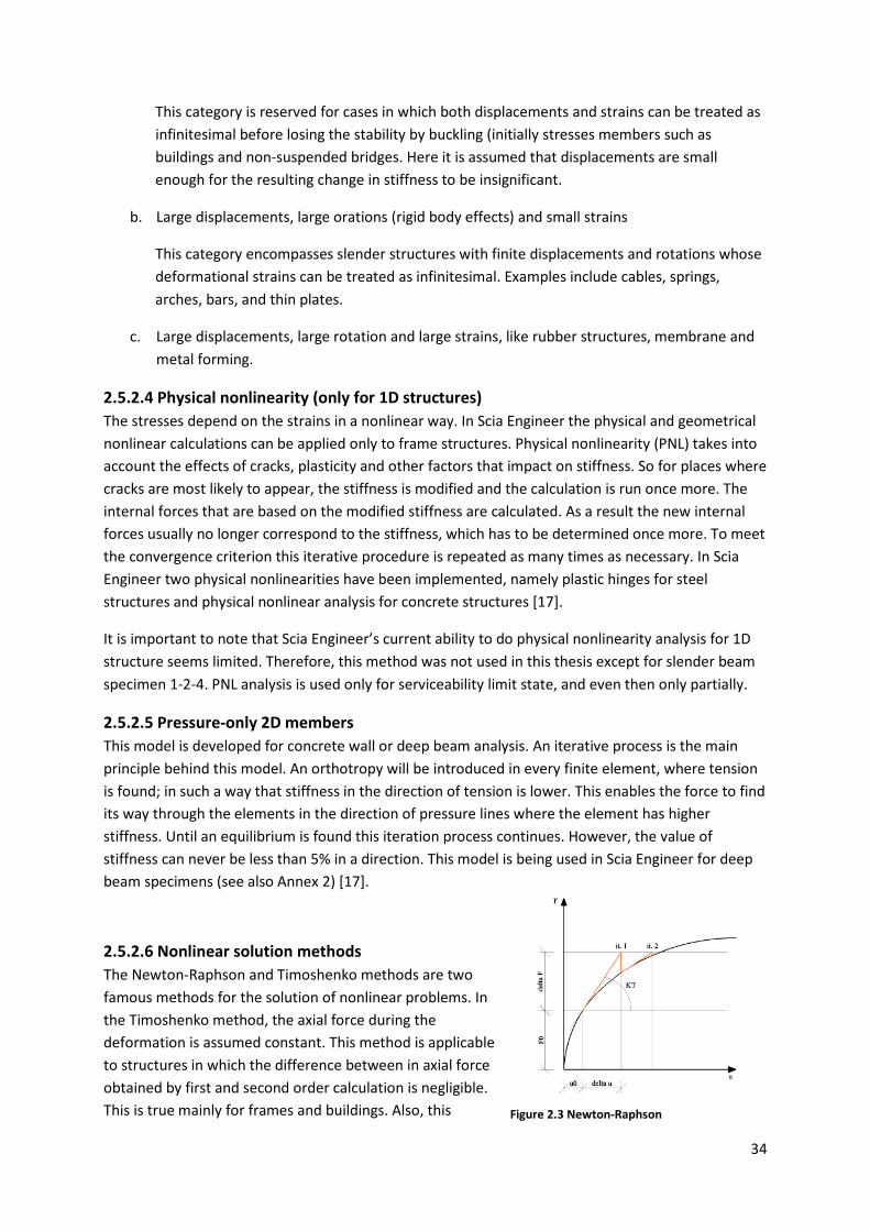
2.5.2.6 Nonlinear solution methods The Newton-Raphson and Timoshenko methods are two famous methods for the solution of nonlinear problems. In the Timoshenko method, the axial force during the deformation is assumed constant. This method is applicable to structures in which the difference between in axial force obtained by first and second order calculation is negligible. This is true mainly for frames and buildings. Also, this Figure 2.3 Newton-Raphson

35
method assumes small rotations and small strains. On the other hand, Newton-Raphson method is very solid and more general for most cases. It can be used for very large deformations and rotations, but the limitations of small strains are still applicable. In this thesis Newton-Raphson has been chosen for the analysis of nonlinear problems.
2.6 Deep Beams or Walls
2.6.1 Introduction Deep beams are structural elements that frequently occur as transfer structures like transfer girders, pile caps and foundation walls. Because of the small ratio between shear span and height, deep beams behave differently from slender beams. Unlike slender beams, the response from deep beams is characterized by nonlinear strain distributions and a significant direct load transfer from the point of loading to the support area. Due to their large stiffness, deep beams are also highly sensitive to imposed deformations, such as differential support settlements. The shear deformations are not negligible and the conventional beam theory is not able to predict the load distribution in continuous deep beams.
2.6.2 Idealizations According to NEN EN 1992-1-1 cl 5.1.1 (6) a common idealization for structural behavior is plastic behavior (including the strut-and-tie model) and nonlinear behavior.
2.6.3 Analysis methods In relation with nonlinear analysis and structures whose behavior can not any more be idealized by linear elastic behavior, the following methods (which are only used for deep beam specimens) will be used in this thesis;
• Standard Beam Method (SBM), [9] • Strut-and-Tie Method (STM), [13], [14], [16], [18] • Nonlinear analysis using Scia Engineer 2D pressure only, [17] • Nonlinear analysis using ATENA
2.6.3.1 SBM (tie arc method) This method of reinforcing and detailing deep beams is a combined method, as it encompasses Eurocode and Dutch code [9].
SBM Design procedure (figure 2.5)
Step 1: Determine the boundary conditions and the theoretical span Note: The effective span is the distance between places on the beam where moment line is zero. For simply supported slender or deep beams this distance is equal to the distance between two supports where the moments are zero.
Step 2: Determine the shear forces, moments and reaction of supports
Step 3: Determining the mesh reinforcements According to NEN EN 1992-1-1 cl 9.7 (1), or NABY- NEN EN 1992-1-1 cl 9.7 deep beams should
36
normally have an orthogonal reinforcement mesh near each face with a minimum of 𝐴𝑠,𝑑𝑏𝑚𝑖𝑛 which is:
𝐴𝑠,𝑑𝑏𝑚𝑖𝑛=0,001𝐴𝑐 ≥ 150 𝑚𝑚2/𝑚
The distance between two adjacent bars should not exceed 300 mm and twice the deep beam thickness.
Step 4: Determining the flexural reinforcements The amount of reinforcement in deep beams should not be smaller than 𝜌𝑚𝑖𝑛 or 1,25 𝐴𝑠;𝑟𝑒𝑞. The amount of minimum reinforcement in walls is generally is bigger than the design-calculated reinforcements. It is possible to use the second condition, which goes as follows:
Needed tensile reinforcement equals
𝐴𝑠,𝑟𝑒𝑞 = 𝑀𝐸𝑑𝑓𝑦𝑑𝑧
≥ 𝐴𝑠,𝑚𝑖𝑛 ,
𝐴𝑠,𝑚𝑖𝑛 = 𝑀𝑐𝑟𝑎𝑐𝑘𝑓𝑦𝑑𝑧
≤ 1,25 𝑀𝐸𝑑𝑓𝑦𝑑𝑧
,
𝐴𝑠,𝑚𝑖𝑛 = 1,25
𝑀𝐸𝑑
𝑓𝑦𝑑𝑧
In these three formulas, z can be determined based on NABY NEN-EN 1992-1-1 cl6.1 (10) or NEN 6720 cl 8.1.4. For statically determined structures the formula goes as follows:
𝑧 = 0,2𝑙 + 0,4ℎ ≤ 0,6𝑙 𝑧 ≤ 0,8𝑙
Step 5: Placing the reinforcement Eurocode contains no information about reinforcement placing in deep beams, which is done according to NEN 6720 cl 9.11.3 (a). The tensile reinforcements are distributed over a specific height, which is the lowest value of 0.2l and 0.2h.
Step 6: Check the anchorage length Anchorage length is checked on the basis of NEN EN 1992-1-1 cl 8.4.3 and 8.4.4.
𝑙𝑏,𝑟𝑞𝑑 = (∅4
)(𝜎𝑠𝑑𝑓𝑏𝑑
)
𝑙𝑏𝑑 = 𝛼1𝛼2𝛼3𝛼4𝛼5𝑙𝑏,𝑟𝑞𝑑 ≥ 𝑙𝑏,𝑚𝑖𝑛 𝑓𝑏𝑑 = 2,25 𝑓𝑐𝑡𝑑
𝑙𝑏,𝑟𝑞𝑑 𝑖𝑠 𝑡ℎ𝑒 𝑏𝑎𝑠𝑖𝑐 𝑟𝑒𝑞𝑢𝑖𝑟𝑒𝑑 𝑎𝑛𝑐ℎℎ𝑜𝑟𝑎𝑔𝑒 𝑙𝑒𝑛𝑔ℎ𝑡 𝑖𝑛 𝑚𝑚 ∅ 𝑖𝑠 𝑡ℎ𝑒 𝑏𝑎𝑟 𝑑𝑖𝑎𝑚𝑒𝑡𝑒𝑟 𝑖𝑛 𝑚𝑚 𝜎𝑠𝑑 𝑖𝑠 𝑡ℎ𝑒 𝑑𝑒𝑠𝑖𝑔𝑛 𝑠𝑡𝑟𝑒𝑠𝑠 𝑜𝑓 𝑡ℎ𝑒 𝑏𝑎𝑟 𝑎𝑡 𝑡ℎ𝑒 𝑎𝑛𝑐ℎ𝑜𝑟𝑎𝑔𝑒 𝑝𝑜𝑠𝑡𝑖𝑜𝑛 𝑓𝑏𝑑 𝑖𝑠 𝑡ℎ𝑒 𝑑𝑒𝑠𝑖𝑔𝑛 𝑣𝑎𝑙𝑢𝑒 𝑜𝑓 𝑢𝑙𝑡𝑖𝑚𝑎𝑡𝑒 𝑏𝑜𝑛𝑑 𝑠𝑡𝑟𝑒𝑠𝑠 𝑓𝑐𝑡𝑑 𝑖𝑠 𝑡ℎ𝑒 𝑑𝑒𝑠𝑖𝑔𝑛 𝑣𝑎𝑙𝑢𝑒 𝑜𝑓 𝑐𝑜𝑛𝑐𝑟𝑒𝑡𝑒 𝑡𝑒𝑛𝑠𝑖𝑙𝑒 𝑠𝑡𝑟𝑒𝑛𝑔𝑡ℎ
𝑙𝑏,𝑚𝑖𝑛 ≥ max �0,3𝑙𝑏,𝑟𝑞𝑑;10∅; 100𝑚𝑚�
Step 7: Check the shear reinforcements using formulas according to NEN EN 1992-1-1 cl6.2.2 and cl6.2.3. This way, one can determine the amount of shear reinforcement that is needed.
𝑉𝑅𝑑,𝑐 = �𝐶𝑅𝑑,𝑐𝑘(100𝜌𝑙𝑓𝑐𝑘)1/3 + 𝑘1𝜎𝑐𝑝�𝑏𝑤𝑑 ≥ (𝑉𝑚𝑖𝑛 + 𝑘1𝜎𝑐𝑝)𝑏𝑤𝑑
𝑉𝑚𝑖𝑛 = 0,0035𝐾3/2𝑓𝑐𝑘1/2

37
𝑘 = 1 + �200𝑑≤2,0
𝜌𝑙 =𝐴𝑠𝑙𝑏𝑤𝑑
≤ 0,02
𝑉𝑅𝑑,𝑠 =𝐴𝑠𝑤𝑠𝑧𝑓𝑦𝑤𝑑𝑐𝑜𝑡𝜃
𝑉𝑅𝑑,𝑚𝑎𝑥 = 𝛼𝑐𝑤𝑏𝑤𝑧𝑣1𝑓𝑐𝑑/(𝑐𝑜𝑡𝜃 + 𝑡𝑎𝑛𝜃)
𝛼𝑐𝑤 and 𝑣1 are 1,0 𝐴𝑠𝑤 is the cross-sectional area of the shear reinforcement S is the spacing of the stirrups 𝑓𝑦𝑤𝑑 is the design yield strength of the shear reinforcement 1 ≤ 𝑐𝑜𝑡𝜃 ≤ 2,5 Step 8: Checking the crack width and crack formation, this can be determined according to NEN EN 1992-1-1 cl 7.3.3 and cl 7.3.4
𝑊𝑘 = 𝑆𝑟,𝑚𝑎𝑥
⎝
⎛𝜎𝑠 − 𝑘𝑡
𝑓𝑐𝑡,𝑒𝑓𝑓𝜌𝑝,𝑒𝑓𝑓
�1 + 𝑎𝑒𝜌𝑝,𝑒𝑓𝑓�
𝐸𝑠≥ 0,6
𝜎𝑠𝐸𝑠⎠
⎞
𝑆𝑟,𝑚𝑎𝑥 is the maximum crack spacing 𝜎𝑠 is the steel stress in the tension reinforcement in SLS, which can be calculated as follows:
𝜎𝑠𝑑 =𝑀𝑆𝐿𝑆
𝑧 ∙ 𝐴𝑠
𝑧 can be found by doing step 4.
𝑘𝑡 is a factor that depends on the duration of the load short term 0.6 and long term 0.4.
2.6.3.2 STM In engineering, the strut-and-tie model (STM) is considered the appropriate basis for the design of cracked reinforced concrete beams loaded in bending, shear and torsion. This method was presented by Schlaich in 1987 and also included in the text by Collins and Mitchell in 1991 and MacGregor in 1992. The strut-and-tie model is a unified approach that considers all load effects for moment, torsion, and axial and shear force. The STM has also the capability to predict more accurately the shear strength of the beams for which a/d is less than 2.5. This method is used also for shear design of disturbed regions. The STM design procedure and the complete definitions can be found in ACI 318-02 Appendix A. In Eurocode NEN EN 1992-1-1 cl 6.5, only the general design procedure for designing strut, ties and nodes is given. Eurocode lacks extensive coverage of the STM design procedures.

38
Definitions
• Hydrostatic nodes: Hydrostatic nodes are loaded with the stress that is applied perpendicularly to each face of the node. This stress is equal in magnitude on all faces of the node.
• B region (Bernoulli region): a portion of a member in which the plane sections assumption of flexure theory can be applied.
• D region (Discontinuity region): abrupt change in geometry or load. St Venant’s principle indicates that stresses due to axial load and bending approaches a linear distribution at a distance approximately equal to the height of the member. For this reason, discontinuity assumes an extension of distance h from the section where the load or change in geometry occurs.
Figure 2.4 Loading and geometric discontinuities [18]
According to NEN En 1992-1-1 cl 5.6.4, a strut and tie model may be used under the following conditions:
• For design in ULS in continuity regions and for the design in ULS and detailing of discontinuity regions.
• Verification in SLS may also be carried out using strut-and-tie models. Here the position and direction of important struts should be oriented in accordance with linear elasticity theory (SBM). This means that another strut-and-tie model should be constructed for SLS. For example, in a single triangular strut and tie model in SLS, the value z should be used the height of the triangle. (Figure 2.5). The important difference is the angle between compression struts and tie. This angle in STM in SLS is smaller, which leads to bigger steel stresses and consequently to bigger cracks. Theoretically, the reinforcement results from STM in crack width calculations should be approximately the same as in SBM.

39
Figure 2.5 STM in SLS (left) and STM in ULS (right)
Possible means to develop suitable strut and tie models include stress trajectories and distributions from linear-elastic theory or the load path model. All strut and tie models may be optimized by energy criteria.
Design procedure
Step 1: Separate B and D regions: with the help of St Venant’s principle one can easily distinguish B and D regions in the structure.
Step 2: Run linear analysis and determine the stress trajectories in the structure [14]: this step is highly recommended, especially for unexperienced engineers. For more accurate results one can also run the NL-FEM with the help of Scia Engineer, but this is more complicated.
Step 3: Make a strut-and-tie model: with the help of step 3, one can simply develop a strut-and-tie model that gives a good estimate of the flow of forces.
Important considerations
Compression struts have two functions in the STM:
1. They serve as the compression chord of the truss mechanism that resists moment
2. They serve as the diagonal struts that transfer shear to the supports.
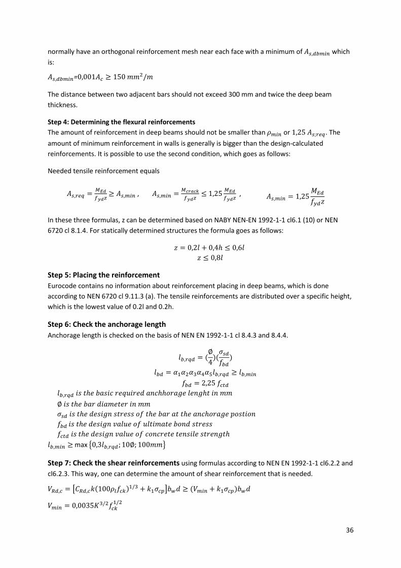
There are three types of struts
1. The simplest type is the ‘prism’, which has a constant width. In this thesis all struts are assumed to be prisms.
2. The second form is the ‘bottle’ in which the struts expands or contracts along its length.
3. The final form is the ‘fan’, where an array of struts with varying inclinations meet at or radiate from a single node.
40
Figure 2.6 Prism (left), fan (middle) and bottle shape (right) struts
Step 4: Make an assumption of strut and tie widths and of the dimension of nodes
Step 5: Perform nodal strength checks (strut and tie widths) according to NEN EN 1992-1-1 cl 6.5
Important considerations
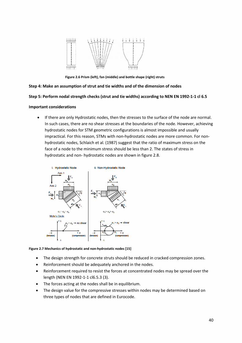
• If there are only Hydrostatic nodes, then the stresses to the surface of the node are normal. In such cases, there are no shear stresses at the boundaries of the node. However, achieving hydrostatic nodes for STM geometric configurations is almost impossible and usually impractical. For this reason, STMs with non-hydrostatic nodes are more common. For non-hydrostatic nodes, Schlaich et al. (1987) suggest that the ratio of maximum stress on the face of a node to the minimum stress should be less than 2. The states of stress in hydrostatic and non- hydrostatic nodes are shown in figure 2.8.
Figure 2.7 Mechanics of hydrostatic and non-hydrostatic nodes [15]
• The design strength for concrete struts should be reduced in cracked compression zones. • Reinforcement should be adequately anchored in the nodes. • Reinforcement required to resist the forces at concentrated nodes may be spread over the
length (NEN EN 1992-1-1 cl6.5.3 (3). • The forces acting at the nodes shall be in equilibrium. • The design value for the compressive stresses within nodes may be determined based on
three types of nodes that are defined in Eurocode.

41
C-C-C Node
𝜎𝑅𝑑,𝑚𝑎𝑥 = 𝑘1𝑣′𝑓𝐸𝑐𝑑 𝑘1 = 1.0
C-C-T Node
𝜎𝑅𝑑,𝑚𝑎𝑥 = 𝑘2𝑣′𝑓𝐸𝑐𝑑 𝑘2 = 0.85
C-T-T Node
𝜎𝑅𝑑,𝑚𝑎𝑥 = 𝑘3𝑣′𝑓𝐸𝑐𝑑 𝑘3 = 0.75
T-T-T Node (Schlaich 1987)
Figure 2.11
• According to NEN-EN 1992-1-1 cl. 6.5.4 (5) the design compressive stress value may be increased by 10% under the following conditions:
o Triaxial compression is assured o All angles between struts and ties are bigger than 55 degrees o The stresses applied at supports or at point loads are the same, and the node
is confined by stirrups
Figure 2.8
Figure 2.9
Figure 2.10

42
o The reinforcement is arranged in multiple layers o The node is reliably confined by means of bearing arrangement or friction
Step 6: calculate required reinforcements in the ties
𝐴𝑠,𝑡𝑖𝑒[𝑚𝑚2] =𝐹𝑡𝑖𝑒 [𝑁]
𝜎𝑦𝑖𝑒𝑙𝑑−𝑠𝑡𝑒𝑒𝑙[𝑁
𝑚𝑚2]
Step 7: calculate required anchorage length according to NEN EN 1992-1-1 cl 8.4.3 and cl 8.4.4. [Step 6 SBM design procedure]
After using Eurocode to find the necessary anchorage length, the available length for anchoring the tensile ties can be estimated using ACI 318-08. According to ACI 318-08 cl A.4.3.1, “nodal zones shall develop the difference between tie force on one side of the node and the tie force on the other side”. The reinforcement in the tie should be anchored before it leaves the extended nodal zone at the intersection of the centroid of the bars in the tie and the extensions of the outlines of either the strut or the bearing area (see figure 2.12).
Step 8: perform crack control checks in the ties according to NEN EN 1992-1-1 cl 7.3.3 and cl 7.3.4. (see Step 8 SBM design procedure)
Complementary step: perform shear check according to step 3 and step 7 from SBM
The literature contains many different flowcharts for the STM procedure. In the figures 2.12 and 2.13 two examples of different flowcharts are visualized. In spite of the different flowcharts for STM, the main principles are the same. One always can optimize these flowcharts for the best optimum use.
Figure 2.12

43
2.6.3.3 NL-FEM 2D pressure only Design Procedure [17]
1. Definition of material properties 2. In the funtionality tab, press-only 2D members for nonlinearity should be chosen. 3. Defining the geometry and support conditions 4. Defining the load combinations 5. Putting Ribs (reinforcement bars) into the 2D pressure only member 6. Refinement of the mesh (number of tiles of 1D member data) 7. Running the nonlinear calculation using SSM (Step by Step Method)
A detailed example of a design procedure can be found in Annex 2.
2.6.3.4 Physical nonlinearity (1D structures) Design Procedure
1. Definition of material properties 2. Input of the structure model including load and boundary conditions 3. Input of member-related parameters 4. Refinement of the mesh (number of tiles of 1D member data)
Figure 2.14 STM tree diagram[13] Figure 2.13 STM tree diagram [15]
44
5. Linear calculation to be able to design or provide input for the reinforcement 6. Design or input of reinforcement 7. Defining nonlinear load combination 8. Non-linear calculation 9. Review and assessment of results
An detailed example of a design procedure can be found in Annex 2 [21].
References
[1] “Plates and FEM surprised and Pitfalls”, Solid Mechanics and its applications Volume 171, Johan Blaauwendraad, professor Emeritus of Structural Mechanics, TU Delft, The Netherlands 2010
[2] “Finite-element Design of Concrete Structures”, Practical problems and their solutions, Second edition, G.A. Rombach University of Hamburg, Hamburg, 2011
[3] Eurocode 2: Design of concrete structures Part 1-1: General rules and rules for buildings NEN-EN-1992-1-1
[4] Eurocode 2: Design of concrete structures, Concrete bridges –design and detailing rules EN-1992-2-2
[5] www.Colorado.edu
[6] “Design of walls with linear elastic finite element methods” Mark Romans, April 2010, TU Delft, concrete structures
[7] Theory Scia Engineer “design of concrete structures” 2008
[8] “Plates and slabs” Prof.dr.ir. J. Blaauwendraad volume 1 theory CT3130, Department of mechanics, materials and structures, section of structural Mechanics, TU-delft, July 2003
[9] Ontwerp in Gewapend Beton, studieboek voor het HBO, de opleiding Bouwkunde en Civiele Techniek, dr.ir.drs. C.D. Braam
[10] Nielsen, M.P., Limit Analysis and Concrete Plasticity, 2nd ed., CRC Press, Boca Raton, London, New York, Washington DC, 1998.
[11] Wood R.H., The reinforcement of slabs in accordance with field of moments, Concrete Mag. 2, 1968, 69–75.
[12] Nonlinear Finite Element Analysis, Script of lectures, dr.ing. Vladimit Ivanco, PhD, Faculty of Mechanical Engineering, TU- Kosice, Slovakia, June 2011
[13] Strut-and-Tie Model Design Examples for Bridges: Final Report, Chris Williams, Dean Deschenes, Oguzhan Bayrak, The University of Texas at Austin, June 2012
[14] Strut-and-Tie Modeling following AASHTO LRFD, Trevor Pullen, Master of Scence, Civil Engineering, Structural Engineering, January 2013
45
[15] Verification of Implementation of Strut-and-Tie Model in LRFD Bridge Design Specifications, requested by AASHTO, November 2007
[16] The Strut and Tie Model of concrete structures, Dr. C. C. Fu, Ph.D., P.E, THE BEST Center University of Maryland, August 2001
[17] Advanced Concept Training, Reinforced concrete (EN 1992)- Adv. Modules, Scia Engineer, 2011
[18] ACI 318-08, Building Code Requirement for Structural Concrete, January 2008.
[20] Theory Physical and Geometrical Nonlinear Analysis of Frame Structures, Scia Engineer, 2006

46
Chapter 3 Linear Elastic and Nonlinear Finite Element Method (specifications)
3.1 Summary This chapter will address the definitions of the geometry of specimens, support conditions and all material properties that are going to be used in remainder of this thesis. All descriptions of geometrical and material properties are based on Eurocode. This chapter also describes various types of load and load combinations and makes suggestions for the incorporation of these data into the LE-FEM software package.
3.2 Slender and Deep Beams
3.2.1 Introduction This thesis is focused on relatively basic, statically determined single-span structures. Slender beams will be examined first, and then deep beams. The relevant theories have already been introduced in the previous chapter. This chapter deals with the following model specifications:
• Dimension • Type and place of loads • Concrete properties • Reinforcements • Supports
3.2.2 Geometry of specimens In this section the geometry of the different specimens based on Eurocode, American code and some other research results will be determined and discussed. According to NEN-EN-1992-1-1 cl. 5.3.1 (3), a beam is a member for which the span to overall depth ratio is bigger or equal to 3 [2].
𝐿ℎ≥ 3 Normal Slender Beam
𝐿ℎ
< 3 Deep beam
According to ACI 318-08: 2007 cl.10.7.1, deep beams have a clear span to overall depth ratio equal to or less than 4. Deep beams can have regions with concentrated loads up to twice the member depth from the face of the support [4].
𝐿ℎ
< 4
Or 𝑎ℎ
< 2
In beams under point load in the center 𝑎 = 𝐿2

47
According to the ACI Structural Journal there are two categories of Deep Beams [7],[4]
• a/d <1,0 • 1<a/d<4
In beams with only one point load at the middle is a=L/2 and ‘d’ can be approximated as ‘h’, which is the height of the beam.
• Lh
< 2 Deep beams are commonly assumed to transfer the total load through tie and arch action[7]
• 2 < L
h< 8 Deep beams transfer loads through a
combination of both ‘tie and arch’ and ‘truss action’ mechanisms.
• 𝐿
ℎ> 8 for slender beams [7]
According to Sergio and Nathan [7], who base their findings on ACI 318-08[4], deep beams with a/d ratios of less than 1 are commonly assumed to transfer the total load through tie-arch action. For slender beams with a/d ratios higher than 4 load transfer mechanism is based on truss action. Loads in deep beams with a/d ratios between 1 and 4 are transferred through a combination of these two mechanisms. EN-1992-1-1 cl. 9.6.1 holds that reinforced walls should have a length-to-thickness ratio of 4 or higher and that the reinforcement should be into account in the strength analysis.
𝐿𝑑≥ 4
In this formula, ‘d’ stands for the thickness of the concrete element.
Rombach [5] claims that shear walls are continuously supported plane members loaded by normal forces. The maximum width of the cross section (l or h) is more than 4 times its minimum width (l or h > 4t). If this is not the case, the member
is column (figure 3.3), which corresponds with NEN-EN 1992-1-1 cl.9.6.1.
Deep beams are plane members that are not continuously supported and whose height (h) is more than half their effective span (𝑙𝑒𝑓𝑓). This is almost in accordance with Eurocode NEN-EN 1992-1-1 cl.5.3.1.
Figure 3.1 Tie arch action
Figure 3.2 Truss action
Figure 3.3 Geometric difference between shear walls and deep beams [5]
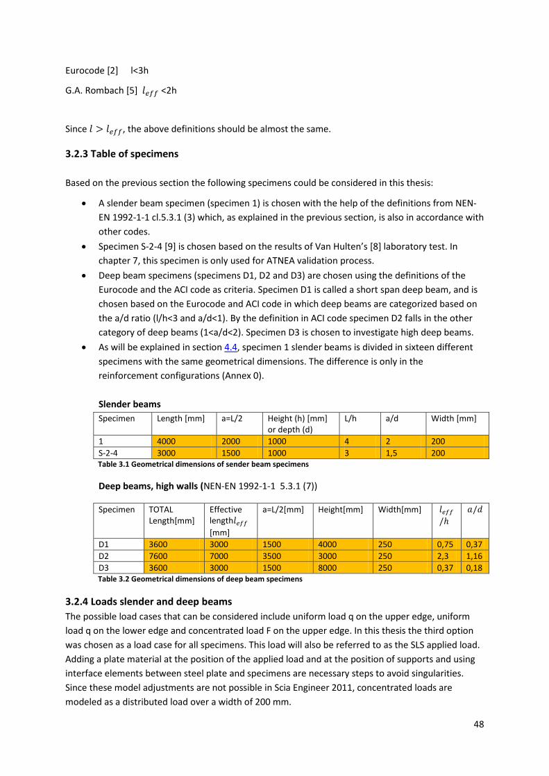
48
Eurocode [2] l<3h
G.A. Rombach [5] 𝑙𝑒𝑓𝑓 <2h
Since 𝑙 > 𝑙𝑒𝑓𝑓, the above definitions should be almost the same.
3.2.3 Table of specimens Based on the previous section the following specimens could be considered in this thesis:
• A slender beam specimen (specimen 1) is chosen with the help of the definitions from NEN-EN 1992-1-1 cl.5.3.1 (3) which, as explained in the previous section, is also in accordance with other codes.
• Specimen S-2-4 [9] is chosen based on the results of Van Hulten’s [8] laboratory test. In chapter 7, this specimen is only used for ATNEA validation process.
• Deep beam specimens (specimens D1, D2 and D3) are chosen using the definitions of the Eurocode and the ACI code as criteria. Specimen D1 is called a short span deep beam, and is chosen based on the Eurocode and ACI code in which deep beams are categorized based on the a/d ratio (l/h<3 and a/d<1). By the definition in ACI code specimen D2 falls in the other category of deep beams (1<a/d<2). Specimen D3 is chosen to investigate high deep beams.
• As will be explained in section 4.4, specimen 1 slender beams is divided in sixteen different specimens with the same geometrical dimensions. The difference is only in the reinforcement configurations (Annex 0). Slender beams Specimen Length [mm] a=L/2 Height (h) [mm]
or depth (d) L/h a/d Width [mm]
1 4000 2000 1000 4 2 200 S-2-4 3000 1500 1000 3 1,5 200
Table 3.1 Geometrical dimensions of sender beam specimens
Deep beams, high walls (NEN-EN 1992-1-1 5.3.1 (7))
Specimen TOTAL Length[mm]
Effective length𝑙𝑒𝑓𝑓 [mm]
a=L/2[mm] Height[mm] Width[mm] 𝑙𝑒𝑓𝑓/ℎ
𝑎/𝑑
D1 3600 3000 1500 4000 250 0,75 0,37 D2 7600 7000 3500 3000 250 2,3 1,16 D3 3600 3000 1500 8000 250 0,37 0,18 Table 3.2 Geometrical dimensions of deep beam specimens
3.2.4 Loads slender and deep beams The possible load cases that can be considered include uniform load q on the upper edge, uniform load q on the lower edge and concentrated load F on the upper edge. In this thesis the third option was chosen as a load case for all specimens. This load will also be referred to as the SLS applied load. Adding a plate material at the position of the applied load and at the position of supports and using interface elements between steel plate and specimens are necessary steps to avoid singularities. Since these model adjustments are not possible in Scia Engineer 2011, concentrated loads are modeled as a distributed load over a width of 200 mm.
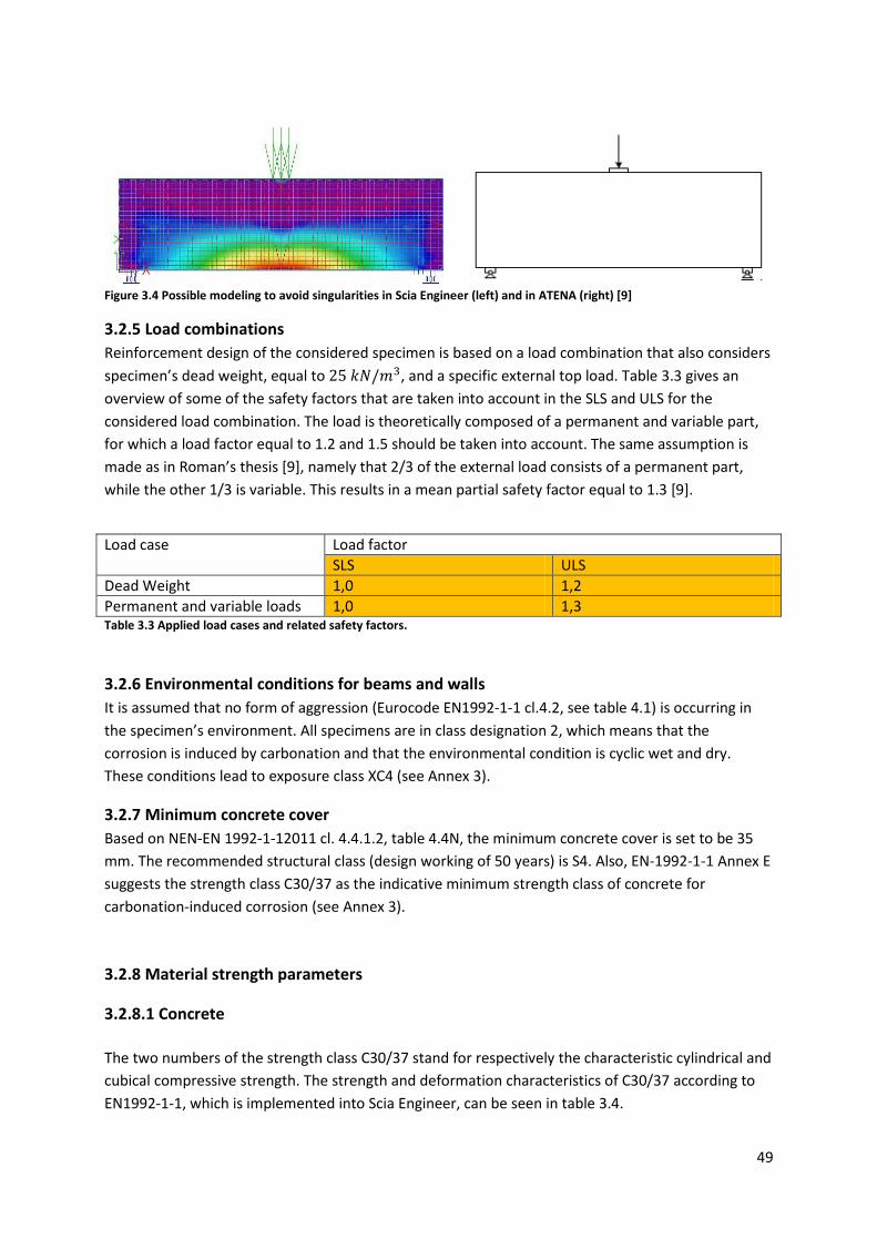
49
Figure 3.4 Possible modeling to avoid singularities in Scia Engineer (left) and in ATENA (right) [9]
3.2.5 Load combinations Reinforcement design of the considered specimen is based on a load combination that also considers specimen’s dead weight, equal to 25 𝑘𝑁/𝑚3, and a specific external top load. Table 3.3 gives an overview of some of the safety factors that are taken into account in the SLS and ULS for the considered load combination. The load is theoretically composed of a permanent and variable part, for which a load factor equal to 1.2 and 1.5 should be taken into account. The same assumption is made as in Roman’s thesis [9], namely that 2/3 of the external load consists of a permanent part, while the other 1/3 is variable. This results in a mean partial safety factor equal to 1.3 [9].
Load case Load factor SLS ULS
Dead Weight 1,0 1,2 Permanent and variable loads 1,0 1,3 Table 3.3 Applied load cases and related safety factors.
3.2.6 Environmental conditions for beams and walls It is assumed that no form of aggression (Eurocode EN1992-1-1 cl.4.2, see table 4.1) is occurring in the specimen’s environment. All specimens are in class designation 2, which means that the corrosion is induced by carbonation and that the environmental condition is cyclic wet and dry. These conditions lead to exposure class XC4 (see Annex 3).
3.2.7 Minimum concrete cover Based on NEN-EN 1992-1-12011 cl. 4.4.1.2, table 4.4N, the minimum concrete cover is set to be 35 mm. The recommended structural class (design working of 50 years) is S4. Also, EN-1992-1-1 Annex E suggests the strength class C30/37 as the indicative minimum strength class of concrete for carbonation-induced corrosion (see Annex 3).
3.2.8 Material strength parameters
3.2.8.1 Concrete The two numbers of the strength class C30/37 stand for respectively the characteristic cylindrical and cubical compressive strength. The strength and deformation characteristics of C30/37 according to EN1992-1-1, which is implemented into Scia Engineer, can be seen in table 3.4.
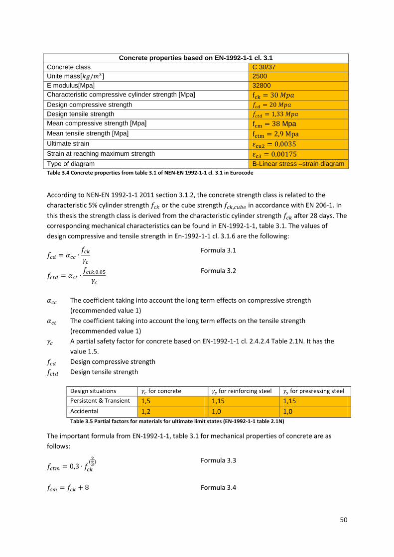
50
Concrete properties based on EN-1992-1-1 cl. 3.1
Concrete class C 30/37 Unite mass[𝑘𝑔/𝑚3] 2500 E modulus[Mpa] 32800 Characteristic compressive cylinder strength [Mpa] fck = 30 𝑀𝑝𝑎 Design compressive strength 𝑓𝑐𝑑 = 20 𝑀𝑝𝑎 Design tensile strength 𝑓𝑐𝑡𝑑 = 1,33 𝑀𝑝𝑎 Mean compressive strength [Mpa] fcm = 38 Mpa Mean tensile strength [Mpa] fctm = 2,9 Mpa Ultimate strain εcu2 = 0,0035 Strain at reaching maximum strength εc3 = 0,00175 Type of diagram B-Linear stress –strain diagram Table 3.4 Concrete properties from table 3.1 of NEN-EN 1992-1-1 cl. 3.1 in Eurocode
According to NEN-EN 1992-1-1 2011 section 3.1.2, the concrete strength class is related to the characteristic 5% cylinder strength 𝑓𝑐𝑘 or the cube strength 𝑓𝑐𝑘,𝑐𝑢𝑏𝑒 in accordance with EN 206-1. In this thesis the strength class is derived from the characteristic cylinder strength 𝑓𝑐𝑘 after 28 days. The corresponding mechanical characteristics can be found in EN-1992-1-1, table 3.1. The values of design compressive and tensile strength in En-1992-1-1 cl. 3.1.6 are the following:
𝑓𝑐𝑑 = 𝛼𝑐𝑐 ∙𝑓𝑐𝑘𝛾𝑐
Formula 3.1
𝑓𝑐𝑡𝑑 = 𝛼𝑐𝑡 ∙𝑓𝑐𝑡𝑘,0.05
𝛾𝑐
Formula 3.2
𝛼𝑐𝑐 The coefficient taking into account the long term effects on compressive strength
(recommended value 1) 𝛼𝑐𝑡 The coefficient taking into account the long term effects on the tensile strength
(recommended value 1) 𝛾𝑐 A partial safety factor for concrete based on EN-1992-1-1 cl. 2.4.2.4 Table 2.1N. It has the
value 1.5. 𝑓𝑐𝑑 Design compressive strength 𝑓𝑐𝑡𝑑 Design tensile strength
Design situations 𝛾𝑐 for concrete 𝛾𝑠 for reinforcing steel 𝛾𝑠 for presressing steel Persistent & Transient 1,5 1,15 1,15 Accidental 1,2 1,0 1,0
Table 3.5 Partial factors for materials for ultimate limit states (EN-1992-1-1 table 2.1N)
The important formula from EN-1992-1-1, table 3.1 for mechanical properties of concrete are as follows:
𝑓𝑐𝑡𝑚 = 0,3 ∙ 𝑓𝑐𝑘(23)
Formula 3.3
𝑓𝑐𝑚 = 𝑓𝑐𝑘 + 8
Formula 3.4
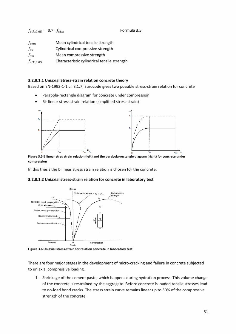
51
𝑓𝑐𝑡𝑘;0.05 = 0,7 ∙ 𝑓𝑐𝑡𝑚 Formula 3.5
𝑓𝑐𝑡𝑚 Mean cylindrical tensile strength 𝑓𝑐𝑘 Cylindrical compressive strength 𝑓𝑐𝑚 Mean compressive strength 𝑓𝑐𝑡𝑘;0.05 Characteristic cylindrical tensile strength
3.2.8.1.1 Uniaxial Stress-strain relation concrete theory Based on EN-1992-1-1 cl. 3.1.7, Eurocode gives two possible stress-strain relation for concrete
• Parabola-rectangle diagram for concrete under compression • Bi- linear stress strain relation (simplified stress-strain)
Figure 3.5 Bilinear stres strain relation (left) and the parabola-rectangle diagram (right) for concrete under compression
In this thesis the bilinear stress strain relation is chosen for the concrete.
3.2.8.1.2 Uniaxial stress-strain relation for concrete in laboratory test
Figure 3.6 Uniaxial stress-strain for relation concrete in laboratory test
There are four major stages in the development of micro-cracking and failure in concrete subjected to uniaxial compressive loading.
1- Shrinkage of the cement paste, which happens during hydration process. This volume change of the concrete is restrained by the aggregate. Before concrete is loaded tensile stresses lead to no-load bond cracks. The stress strain curve remains linear up to 30% of the compressive strength of the concrete.

52
2- If concrete is subjected to stresses greater than 30 to 40% of its compressive strength, the stresses on the inclined surface of the aggregate particles will exceed the tensile and shear strength of the paste-aggregate interfaces. In such cases, new cracks are likely to appear. These so-called bond cracks are stable and develop only if the load increases. After these cracks occur any additional load is redistributed to the remaining intact interfaces and to the mortar. As a result, a gradual bending of the stress-strain curve for stresses above 40 percent of the short time strength may occur.
3- As the load increases above 50 or 60% percent, mortar cracks develop between bond cracks. These cracks develop parallel to the compressive loading and are due to the transverse tensile strains. The start of this stage of loading is called the discontinuity limit.
4- At 75 to 80% of the ultimate load the number of mortar cracks begins to increase. As a result there are fewer intact portions to carry the load, and the stress-strain curve becomes even more nonlinear. The start of this stage of cracking is called critical stress.
3.2.8.1.3 Biaxial loading of uncracked unreinforced concrete Concrete is said to be loaded biaxially when it is loaded in two perpendicular directions with no stress or restraint of deformation in the third direction. This type of stress-strain relation will be explained in the nonlinear analysis. In linear analysis the simplified uniaxial stress strain diagram is used.
Figure 3.7 Strength and modes of failure of unreinforced concrete subjected to biaxial stresses (left) and the biaxial state of stress in the web of a beam (right)
3.2.8.2 Reinforcement
3.2.8.2.1 Reinforcement design using GTB2010, NEN6008 and EN 1992-1-1 Annex C The applied reinforcement quality is B 500B, which typically has a characteristic tensile strength of 500 N/mm2. The corresponding design strength is 435 N/mm2. The table below shows the properties of the reinforcing bars in accordance with NEN-EN 1992-1-1.
Reinforcement type B 500B Specific weight[𝑘𝑔/𝑚3] 7850 E- modulus [MPa] 200000
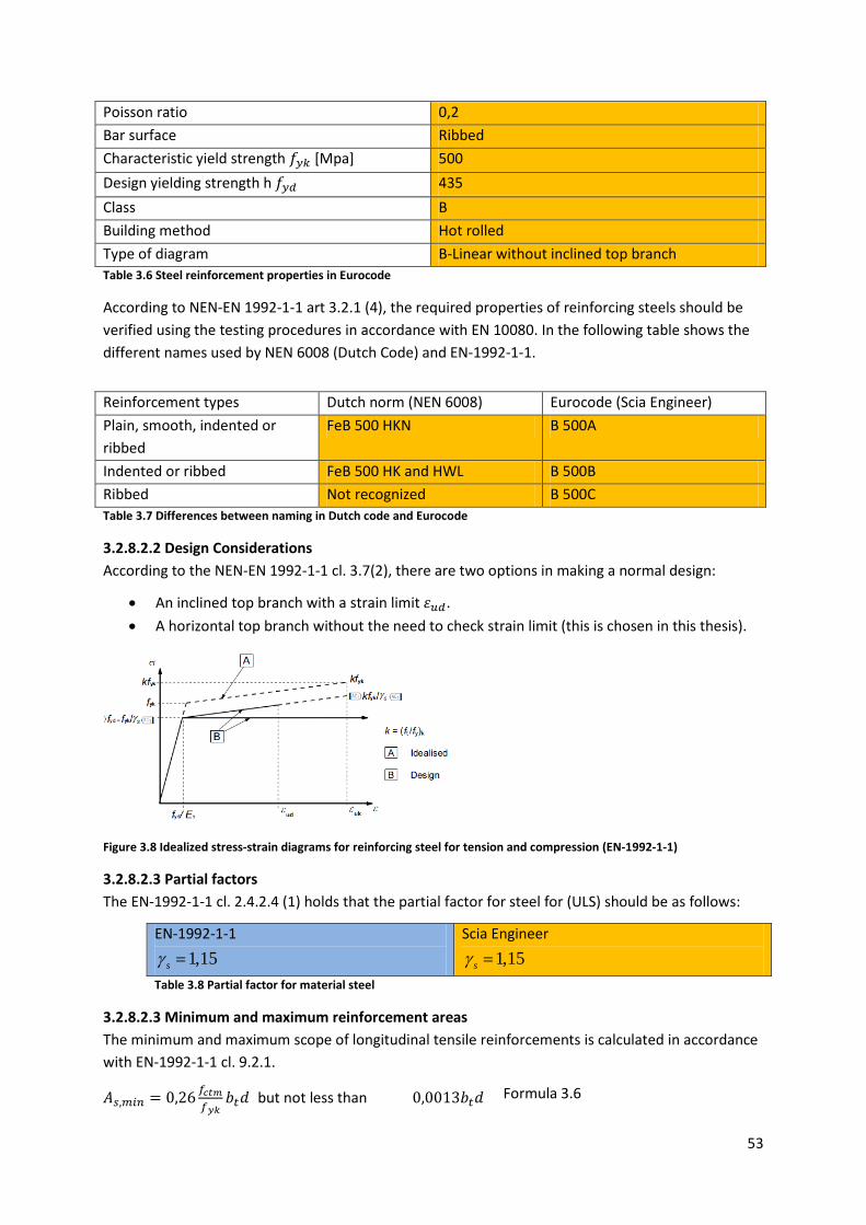
53
Poisson ratio 0,2 Bar surface Ribbed Characteristic yield strength 𝑓𝑦𝑘 [Mpa] 500 Design yielding strength h 𝑓𝑦𝑑 435 Class B Building method Hot rolled Type of diagram B-Linear without inclined top branch Table 3.6 Steel reinforcement properties in Eurocode
According to NEN-EN 1992-1-1 art 3.2.1 (4), the required properties of reinforcing steels should be verified using the testing procedures in accordance with EN 10080. In the following table shows the different names used by NEN 6008 (Dutch Code) and EN-1992-1-1.
Reinforcement types Dutch norm (NEN 6008) Eurocode (Scia Engineer) Plain, smooth, indented or ribbed
FeB 500 HKN B 500A
Indented or ribbed FeB 500 HK and HWL B 500B Ribbed Not recognized B 500C Table 3.7 Differences between naming in Dutch code and Eurocode
3.2.8.2.2 Design Considerations According to the NEN-EN 1992-1-1 cl. 3.7(2), there are two options in making a normal design:
• An inclined top branch with a strain limit 𝜀𝑢𝑑. • A horizontal top branch without the need to check strain limit (this is chosen in this thesis).
Figure 3.8 Idealized stress-strain diagrams for reinforcing steel for tension and compression (EN-1992-1-1)
3.2.8.2.3 Partial factors The EN-1992-1-1 cl. 2.4.2.4 (1) holds that the partial factor for steel for (ULS) should be as follows:
EN-1992-1-1
1,15sγ =
Scia Engineer
1,15sγ = Table 3.8 Partial factor for material steel
3.2.8.2.3 Minimum and maximum reinforcement areas The minimum and maximum scope of longitudinal tensile reinforcements is calculated in accordance with EN-1992-1-1 cl. 9.2.1.
𝐴𝑠,𝑚𝑖𝑛 = 0,26 𝑓𝑐𝑡𝑚𝑓𝑦𝑘
𝑏𝑡𝑑 but not less than 0,0013𝑏𝑡𝑑 Formula 3.6

54
𝐴𝑠,𝑚𝑎𝑥 = 0,04𝐴𝑐 (This will be elaborated on in chapter 5) Formula 3.7
𝑏𝑡 is the mean width of the tension zone 𝑓𝑐𝑡𝑚 is the mean axial tensile strength
𝐴𝑐 Is the area of concrete cross-section
3.2.8.2.4 Curtailment of longitudinal tension reinforcement EN-1992-1-1 cl. 9.2.1.3 (2) holds that the additional tensile force 𝛥𝐹𝑡𝑑 for members with shear reinforcement should be calculated in accordance with NEN-EN 1992-1-1 cl.6.2.3 (7). For members without shear reinforcement 𝛥𝐹𝑡𝑑 maybe estimated by shifting the moment curve a distance 𝑎𝑙 = 𝑑 according to NEN-EN 1992-1-1 cl.6.2.2 (5). This shift rule may also be used as an alternative for members with shear reinforcement where:
𝑎𝑙 = 𝑧(𝑐𝑜𝑡𝜃 − 𝑐𝑜𝑡𝛼)/2 Formula 3.8
Α The angle between shear reinforcement and the beam axis perpendicular to the shear force 𝜃 The angle between the concrete compression strut and the beam axis perpendicular to the
shear force 𝐹𝑡𝑑 The design value of the tensile force in the longitudinal reinforcement 𝐹𝑐𝑑
The design value of the concrete compression force in the direction of the longitudinal member axis
Z The inner level arm
There are two approaches, both of which are implemented in a smart way in Scia Engineer:
1. The ‘shear effect’ approach laid down in EN-1992-1-1 cl.6.2.3 (7) is the default approach used in 2D finite element analysis in Scia Engineer under the name ‘Shear effect considered in SR2’ (see also Annex 4).
2. The classic ‘moment shift’ approach as explained in EN-1992-1-1 cl. 9.2.1.3 (2). This approach is used in ‘hand calculations’ and ‘1D beam models’ (see also Annex 4).
Figure 3.9 Illustration of the curtailment of the longitudinal reinforcement (EN-1992-1-1, figure 9.2)

55
Note: Taking into account the research results of Romans [9], who concludes that there is no direct relation between the observed failure mode and the moment distribution that is no longer shifted, it was decided to focus this thesis on the default values in 2D and 1D modeling in Scia Engineering, which includes the two approaches mentioned above: shear effect and moment shift.
3.2.9 Mesh reinforcement According to NEN-EN 1992-1-1 cl.9.7 (1), deep beams should normally be provided with an orthogonal reinforcement mesh near each face with a minimum amount of:
2, min 0,001 150 /s db cA A mm m= ≥
Note: This is only applicable to deep beam specimens. For slender beam specimens no reinforcement mesh is necessary.
3.2.10 Anchorage of reinforcement for beams The minimum anchorage length may depend on the required anchorage length. This can be calculated when the design value of the tensile stresses in the reinforcement bars is known. As yet, however, this value is unknown.
𝑙𝑏,𝑟𝑞𝑑 = (𝜙4
)(𝜎𝑠𝑑𝑓𝑏𝑑
)
Formula 3.9
𝜙 bar diameter 𝜎𝑠𝑑 the design stress of the bar at the position from which the anchorage is measured 𝑓𝑏𝑑 the design value of the ultimate bond stress (EN-1992-1-1 cl. 8.4.2 (2))
As the first design stress of the bars is not yet available, minimum length of the anchorage can be approximated by using NEN-EN-1992-1-1 cl. 8.4.4(1).
𝑙𝑏,𝑚𝑖𝑛 ≥ 𝑚𝑎𝑥{10𝜙; 100 𝑚𝑚} Formula 3.10
Bar Diameter 𝜙[mm] Anchorage Length [mm]
8 100 10 100 12 120 16 160 Table 3.9 Anchorage lengths in EN-1992-1-1 cl.8.4.4 (1)
Note: Taking into account the anchorage length in Scia Engineer models is considered redundant. For details, see section chapter 5.2.2.3.
3.2.11 Mesh size for beam specimens The 2D finite element models of the considered specimens in Scia Engineer are subdivided into a number of square four nodded finite elements on the basis of which the membrane forces and

56
strains are calculated. Determining mesh density is an important step in finite element modeling. Convergence of the results can be achieved by choosing an adequate number of elements in the models. A practical convergence study was done using Scia Engineer. An overall finite element mesh consisting of square elements of 50 mm turned out to provide adequate analysis results (see Annex 1 for the convergence study).
3.2.12 Supports and loads for beams In many structures the supports are not fully or only partly restrained. Therefore, the deflection at the supports cannot be ignored. Possibilities to model a support include the following [5]:
• Individual spring elements • Special interface elements • Continuous elastic supported elements • Plane or 3D shell or volume elements • Or some combination of above mentioned possibilities
High concentrated point loads on structural elements causes singularities, or infinite stress and internal forces. Simplifications and assumptions of element behavior causes singularity problems in numerical models. For example, in the area of pin support the assumption of linear strain distribution in a slab or beams is not valid. Examples of singularities and ways to avoid them include corners and concentrated loads or pin supports:
1- Corners (free or fully restrained) This could be avoided by positioning of supports at a specific distance from the edges of the beam. For the supports, a free distance of 100 mm is applied between the edge of the beam and the supports. Also, to be able to avoid singularities pin joined supports should be avoided in modeling. It is recommended to use several pin joints close to each other [5].
2- Concentrated loads or pin supports
In Scia Engineer numerical problems can be avoided by applying concentrated load as a distributed load on the certain area, also considering the width of the load area. In real structures singularities do not happen, and in case of high stresses the yielding of the material occurs. In such cases, the concrete in the tensile regions will crack.
Beam support
G.A. Rombach [5] has showed that the stiffness of the supports of statically indeterminate structures must be considered in the design model. In this thesis all specimens are statically determined, so initially there is no need to model the supports with springs, especially for slender beams. As these singularities do not influence the overall reinforcement configuration of the specimens in this thesis, one can simply ignore these singularities. However, it was decided that the following two kinds of support will be used in the models in this thesis.
• Rigid supports
This type of support is used for slender beam specimens, especially for small loads, because at lower loads singularities will not happen. On the other hand, for higher loads the

57
singularities will become more visible. In that case the flexible spring option is better for accurate modeling.
Figure 3.10 E6 (crushing of the concrete error) in Scia Engineer due to the singularities caused by rigid support (left) and flexible support in Scia Engineer (right)
• Spring supports
As mentioned above, to avoid singularities the spring flexible support is a better choice for modeling in a proper manner, especially for higher loads. Beams or deep beams are often supported by columns or walls. To consider the stiffness of the bearing structure, one can model them by using individual springs. There is no need to model the bearing structure, e.g. the column or wall itself. Bending and normal stiffness of the column should both be modeled by individual springs. It is important to know that bending springs cannot be used in conjunction with plane membrane elements, because they have no freedom for rotation.
The axial stiffness of springs 𝐶𝑁 for the column is obtained from the following expression (slender beams).
𝐶𝑁 =𝐸.𝐴𝐶𝐿
Formula 3.11
L Height of the column
3.2.13 Finding axial stiffness for slender beams 𝐸𝑐𝑚 = 33000𝑁/𝑚𝑚2 𝑙 = 3600 𝑚𝑚 𝐴𝑐 = 1000 𝑚𝑚 ∙ 200 𝑚𝑚 𝐶𝑁 = 𝐸𝑐𝑚∙𝐴𝑐
𝑙= 33000∙200∙100
3600= 183000 𝑁
𝑚𝑚 𝑐𝑜𝑛𝑣𝑒𝑟𝑡 𝑡𝑜 𝑆𝑐𝑖𝑎 𝐸𝑛𝑔𝑖𝑛𝑒𝑒𝑟 𝑢𝑛𝑖𝑡 𝑔𝑖𝑣𝑒𝑠1830𝑀𝑁/𝑚2
3.2.14 Finding axial stiffness for deep beams Pile stiffness is assumed to be 1∙ 105 kN/m
The length of the support area is 0,4 m
Stiffness per meter length of the support area 1∙105 kN/m0,4
=250∙ 103kN/𝑚2 or 250 MN/𝑚2
58
3.2.15 Horizontal restraint (general) Horizontal restraints caused by incorrect modeling of the support conditions in beam or deep beam analysis is a really important issue, because they may result in considerable reduction in the design tensile forces. There are two possible support systems.
System 1: both supported are fixed in the vertical direction, and only one support is fixed in the horizontal direction. The use of this system yields realistic results, which is why this system is going to be used in this thesis.
System 2: both supports are fixed in both directions.
References
[1] “Reinforced concrete: mechanics and design”, James G. MacGregor and James K. Wight
[2] Eurocode 2: Design of concrete structures Part 1-1: General rules and rules for buildings NEN-EN-1992-1-1
[3] Eurocode- Basis of structural design NEN-EN-1990 [4] ACI 318-08 “Building Code Requirements for Structural Concrete and Commentary” [5] “Finite-element Design of Concrete Structures”, Practical problems and their
solutions, Second edition, G.A. Rombach University of Hamburg, Hamburg, 2011
[6] NEN Dutch code 6008
[7] “Evaluation of load transfer and strut strength of deep beams with short longitudinal bar anchorages” ACI Structural Journa, Sergio F. Brena and Nathan C. Roy, 2009
[8] Master thesis “Loading capacity of reinforced concrete deep beams”, Bart van Hulten (2011), TU Delft, concrete structures
[9] “Design of walls with linear elastic finite element methods” Mark Romans April 2010, concrete structures
[10] GTB “Grafieken en Tabellen voor Beton” Leading committee: ing. R.Sagel, ir. W.C. Dees, ing. F.P.J van Geest, dr.ir.drs. C.R. Braam, November 2010
59
Chapter 4 Reinforcing the Specimens (LE-FEM & NL-FEM)
4.1 Summary In this chapter background and the theory of the LE-FEM software package used in this thesis will be explained. The LE-FEM software package used in this thesis is Scia Engineer 2011. Knowing the history and the theoretical background of this software is essential for a better understanding of it’s analysis results. At the end of this chapter the process of optimization is introduced and the reader becomes familiar with the methods in this software to reinforce concrete elements. The last part of this chapter will also provide a brief explanation about NL-FEM module of the same software package.
4.2 Introduction This chapter includes the following sections:
• Brief background theory of Scia Engineer • Using Scia to determine longitudinal and vertical reinforcements • Method of reinforcing the specimens
a) Normal method b) Step by Step Method (SSM)
• Comparison between these two methods • Optimization process • How to do reinforcement design of 2D structures in Scia Engineer (see the Annexes 0 to 4) • Reinforcement design with the LE-FEM software package for both slender and deep beams is
the same • Reinforcement design with the NL-FEM software package for deep beams is explained in the
last section of this chapter • Both LE-FEM and NL-FEM is done with the help of Scia Engineer software package
4.3 Design of Reinforcements for Slender and Deep BEAMS in LE-FEM
4.3.1 Introduction to reinforced concrete design of 2D structures in Scia Engineer NEDIM is the generic name for 2D reinforcement concrete design modules PRC.72.xx (ESA-Prima Win or EPW) as well as ESACD.02.xx (SCIA.ESA PT). Both EPW and ESA PT have been using the same NEDIM package, however there are differences in Input/Output handling; ESA PT allows for some additional, more advanced I/O control options. NEDIM has been developed by a group of organizations [1]. The name NEDIM has been chosen to allow for efficient communication between developers, testers and supporters. Three types of analysis can be distinguished by NEDIM: walls, plates and shells. From these, the shell analysis is the most general one.
Shell models can be reduced mechanically to produce plates and walls. The true task of the structural engineer is the creation of FEM model. Scia Engineer is a tool that enables the user to create and manage competent mechanical models by using sub-structure techniques. Such structural parts are also called macro-elements.

60
The aim of the module NEDIM is the reinforcement of concrete design and SLS proofs (crack proof) in compliance with national standards of plates, walls and shell structures. In this thesis the Eurocode with national Annex is chosen in Scia Engineer project properties (see the Annexes 0 through 4].
4.3.2 Features of NEDIM • Processing and reporting of compression reinforcement (the theory of Baumann). • Reliable system of detection of non-design abilities (errors, see also Annex 4) • Ability to deal with 2, 3 course of reinforcement nets almost deliberate geometry.
4.3.3 Transformation of inner forces of the FEM solution to design forces [1] Once the reinforcement design input data is read and analyzed and the FEM data base approached, the NEDIM design model can be created respecting all NORM rules. As has already been mentioned, NEDIM distinguishes between wall, plate and shell analyses. As this thesis is about slender beam specimens, wall elements are chosen in Scia Engineer model.
Estimation of the inner design forces for each item to be designed is the first essential step of the design procedure. Under the actual FEM solver there is only one design item, the finite element node. Inner forces of FEM analysis cannot be used as direct design forces. The inner forces transformation procedure is essential to enable the 2D design. The NEDIM transformation procedure is based on general transformation formula by Baumann (see Annex 4).
𝑐𝑖 =�𝑠𝑖𝑛𝑎𝑗𝑠𝑖𝑛𝑎𝑘 + 𝑘𝑐𝑜𝑠𝑎𝑖𝑐𝑜𝑠𝑎𝑘��𝑠𝑖𝑛(𝑎𝑗 − 𝑎𝑖)𝑠𝑖𝑛(𝑎𝑘−𝑎𝑘)�
(𝑖, 𝑗,𝑘, . . . = 1,2,3,1, … )
Formula 4.1
𝑎𝑖,𝑗,𝑘 angles between individual reinforcement/strut directions and the direction of the first principal membrane force n1 (walls)
k Quotient n2/n1; it can be assumed negative, zero or positive value
𝑐𝑖 transformation coefficient associated with the transformation direction i
In the formula 4.1 the cyclic formula the subscripts i, j, and k denote one of the three reinforcement directions according to figure 4.1 or two reinforcement directions and the direction of the virtual concrete strut.
The design forces 𝑛𝑖 is defined by the following
relation:
𝑛𝑖 = 𝑐𝑖𝑛1
Formula 4.2
Figure 4.1 Reinforcement geometry, upper and lower face [1]

61
The transformation formulas 4.1 and 4.2 in walls transform the basic inner forces [𝑛𝑥 ,𝑛𝑦,𝑛𝑥𝑦]. Basically, the design forces according to the formulas 4.1 and 4.2 meet the following generalized first tensor invariant condition, no matter what model they represent:
𝑛1𝑑 + 𝑛2𝑑 + 𝑛3𝑑 = 𝑛1 + 𝑛2 = 𝑐𝑜𝑛𝑠𝑡
Formula 4.3
In the formula above, 𝑛1 and 𝑛2 are the principal normal forces. The inner forces 𝑛𝑥, 𝑛𝑦, and 𝑛𝑥𝑦 of the FEM solution resulted from the FEM database for each design item, and have been transformed by the method mentioned above into the design forces 𝑛1𝑑 ,𝑛2𝑑 , and 𝑛3𝑑. Once the positive design force has been assigned to its associated reinforcement course, the corresponding statically required reinforcement level 𝑎𝑖 is calculated from the following relation:
𝑎𝑖 = 𝑛𝑖𝜎𝑠𝑑
(i= 1,2, (,3)) Formula 4.4
Important note: With 2D LE-FEM with Scia Engineer the reduction factor for concrete compression strength in the compression struts is taken into account (𝑓𝑐𝑑,𝑟𝑒𝑑 = 0,8𝑓𝑐𝑑). This is due to the cracks parallel to the compression struts. (Annex 4).
4.4 Process of Reinforcing 1. First, by using a 2D finite element model in Scia Engineer the needed reinforcement
configuration is found. Scia Engineer gives its output per element for required reinforcement in 𝑚𝑚2/𝑚. To obtain the actual required reinforcement area 𝐴𝑠 in longitudinal direction, the output must be multiplied by a chosen height of the finite element model. This height is the designer’s choice. The results from different chosen heights should be almost the same. In this thesis the chosen height for slender beam models to determine each layer of reinforcement is about 75 mm. For the vertical direction (shear reinforcements) the output must be multiplied by the chosen length of the finite element model. In this thesis the length is 1 meter [2].
2. For verifications of the reinforcement configuration as a result of a 2D finite element model analysis by Scia Engineer, the reinforcement configuration is applied to a 1D beam model in Scia Engineer.
3. In applying the reinforcement from 2D to 1D model, the following options are examined in this thesis. • Longitudinal and vertical reinforcement is optimized • Only vertical reinforcement is optimized • Reinforcement configuration based on 2D Scia finite element model
4.4.1 Important design considerations in using 2D finite element model
1) To process 2D models, Scia Engineer requires longitudinal reinforcement bars along almost the entire height of the slender beams. This is because of the finite element calculations that are done by Scia in the scale of mesh elements. Scia Engineer calculates the amount of required reinforcements in all mesh elements in the considered beam.

62
2) In Scia Engineer 2D model, there is no possibility to add Stirrups for Shear stresses, so it is decided to just add vertical mesh only. As can be seen in the verification steps by hand and by 1D modeling in Scia, the results are reliable and correct.
4.4.2 Why optimization in SCIA? Annex 4 shows how one can explain how Scia Engineer considers the Eurocode and non-Eurocode rules (in 2D finite element model) to determine the amount of required reinforcements. Also, in the 1D beam model Scia Engineer also takes too many detailing provisions into account.
Consequently theses extra measurements causes conservative results from Scia Engineer both in 2D finite element model and also in 1D beam model. Some errors may occur in the results or capacity checks in the 1D beam model and in the 2D FE model in Scia Engineer which should be studied and if it is necessary they could be ignored (see annex 3 for error explanation). Optimizing the reinforcement configurations is done by ignoring the longitudinal skin (flankwapening) reinforcement or by the application vertical shear reinforcements based on hand calculations or 1D beam models
The linear elastic finite element method (LE-FEM) derives the required reinforcement directly from the membrane forces, which are calculated in individual nodes of the finite element mesh.
4.4.3 Two methods of configurations 1. Normal method, also used by Romans [2]
Generally this method is based on ‘one time reinforcement’. The required reinforcement is given by Scia Engineer. The reinforcement is added to the specimen in one go-time. To apply this method, the following steps should be followed.
• Calculation by Scia Engineer for the required amount of reinforcement • Find required dimensions of reinforcement • Put all necessary reinforcements in the whole specimen in different layers • Let Scia recalculate and check whether more reinforcements are needed • If more reinforcement is needed, one has to through the previous steps again
Note: From the steps mentioned above it seems that this method is iterative, but it is not. The last step is just an adjustment of the reinforcements in one time. The whole process happens only once.
2. New method “Step by Step Method” or SSM [Annex 3]
This method is developed by the author of this thesis. In this method, the general procedure for the calculation of reinforcement, mentioned in the normal method as used by Romans [2], is also valid. This method is based on the behavior of the material and redistribution of stresses after putting each layer of the reinforcements. This method can be formulated as follows:
• Calculation by Scia Engineer • Find dimensions of the required reinforcement at the bottom edge of the specimen, with a
required specific height

63
• Putting one or two bottom reinforcement layers • Calculation by Scia Engineer (again) • Find amount of the required reinforcement at the second or third layer from bottom with a
specific height. • Calculation by Scia Engineer. • User is required to repeat these above steps till the need for more reinforcement is fulfilled
according to the Scia Engineer calculation.
Tip 1: after adding two or three layers of reinforcement, Scia Engineer might require more reinforcement in layer 1 or 2. The user can adjust some parameters of that specific layer, for example by choosing a higher diameter, or by adding extra reinforcements.
Tip 2: At the end of configuration Scia still requires some reinforcements at the bottom edge or top edge of the specimens, but these requirements can be ignored. Scia Engineer calculates the necessary reinforcement for each small finites mesh element. Due to the finite element calculations , the program also proposes reinforcement at the edge of the slender beam. Such suggestions can safely be ignored.
Note: For the first or second layer of longitudinal reinforcements full anchorage is assumed based on the Eurocode and the results of the Romans work.
4.4.3.1 Comparison between two methods of reinforcing: As an example, the new ‘step by step’ method is applied for a specimen under 200 kN loading (Annex 3).
Reinforcement configuration Description 1d1d In which both horizontal and vertical reinforcements are optimized and can be called 1d1d.
1d2d In which only horizontal reinforcements are optimized (1d). Vertical reinforcements are still
based on the (2D) Scia finite element model, and can be called 1d2d.
2d1d In which only vertical reinforcements are optimized (1d). Horizontal reinforcements are still based on the (2D) Scia finite element model, and can be called 2d1d.
2d2d In which none of the horizontal or vertical reinforcements are optimized. They can be called 2d2d (this is derived directly from 2D finite element model in SCIA).
Specimen Applied point load (SLS)[kN] Reinforcement configuration 1-1-1 200 1d1d
1-1-2 1d2d
1-1-3 2d1d
1-1-4 2d2d
Table 4.1 Naming method for specimens based on reinforcement configurations
Specimen Rein. config
Method Steel [𝑘𝑔/𝑚3]
Unity check crack width [-]
Unity check max moment [-]
Unity check max shear [-]
1-1-1 1d1d Normal 80 0,76 0,44 0,59 Step by Step 80.6 0,66 0,46 0,61
Table 4.2 Analysis results for Normal and step by step method for specimen 1-1-1

64
Two preliminary observations can be made. First, from looking at the unity checks it is clear that initially both methods give the same results for moment and shear capacity. Second, both methods use roughly the same amount of steel. Initially here means without any more optimization. For example, for shear reinforcement it is always possible to place the shear reinforcements more efficiently (more rebars near supports and fewer rebars in the middle). However, the smart placement of the shear reinforcements will not be considered here. Reinforcing according to the ‘normal’ method needs more trial and error before it becomes a feasible option. SSM is faster and more efficient. For instance, less manpower is needed because of its practical approach to detailing, which may involve combining the small reinforcement bars together and placing the rebars in the critical places can be easily achieved.
4.5 Design of Reinforcements in Deep Beams in NL-FEM In this thesis deep beam specimens are reinforced in the LE-FEM and the NL-FEM in Scia Engineer. In the previous section the method of reinforcing in LE-FEM has been discussed. As has been explained in section 2.5.2.4, about the design method of pressure-only members in Scia Engineer, to be able to do the NL-FEM in Scia Engineer, the reinforcing can be done by using steel ribs. This is the big difference with the LE-FEM in Scia Engineer, in which desired reinforcements can be added to the specimens and the program checks whether the specimens need more reinforcement or not. Pressure-only members in Scia Engineer provide the ability to simulate the behavior of deep beams or walls in a more realistic, nonlinear method. It is important to mention that applying ribs is done according to SSM as illustrated in section 4.4.3. The design procedure is illustrated in Annex 2.
4.5.1 Process of reinforcing 1- In Scia Engineer’s nonlinear module the use of reinforcement is no longer possible. Through
engineering logic and the stress trajectories from the LE-FEM, one can decide where to put steel ribs into the specimen. In order to do this, one has to know about the principle behind STM.
2- By running the nonlinear calculations, Scia Engineer gives the amount of forces and stresses in the specimen and in the ribs themselves.
3- A simple calculation is enough to establish the number of reinforcements from the forces in the ribs.
4- Forces are given in KN/m. By multiplying amount of forces in distances in the x and the y direction, one can check whether the specimen needs reinforcements. Note: It is not possible to add mesh net to the model, so the amount of mesh nets should be included into the calculations for needed reinforcements. The amount of mesh nets can be calculated by using NEN EN 1992-1-1 cl 9.7.
5- No verifications of the reinforcement configuration can be done by Scia Engineer. For verification of reinforcement configuration specimens are modeled in ATENA.
65
4.5.2 Important design considerations in using 2D finite element model
1- In 2D models Scia Engineer requires longitudinal reinforcement bars along almost the entire height of the slender beams. This is because of the finite element calculations that are done by Scia in the scale of mesh elements. Scia Engineer calculates the number of required reinforcements in all mesh elements in a given beam.
2- Ribs should be seen as indicators of the reinforcement area. It is recommended to use ribs with a 20 mm diameter in places where tensile stresses are likely to occur.
3- As has is already been mentioned, basic knowledge of STM is essential to use 2D pressure only (nonlinear module).
References
[1] “Theory Design of Concrete Structures” Scia Engineer Group 2008
[2] “Design of walls with linear elastic finite element methods” Mark Romans April 2010, concrete structures

66
Chapter 5 Required Verifications in Limit States
5.1 Summary In this chapter all needed verifications in limit states (both SLS and ULS) are going to be done in accordance with Eurocode. Verification of specimens is done with the help of hand calculation and the 1D beam model in LE-FEM software package. Also, a comparison will be made between hand calculation and Scia’s 1D model. The conclusion is that Scia Engineer’s 1D model can very accurately predict the behavior of the specimen in SLS and ULS. Therefore, in this thesis the Scia Engineer 1D module is used for all slender beam specimens and for analyses in SLS and in ULS. This chapter also contains a brief introduction about PNL analysis for nonlinear 1D beam models. PNL analysis to for analyze slender beams in SLS shows that this module in Scia Engineer can predict the cracking behavior, deflection and stiffness reduction of the specimens.
5.2 Slender Beams Important note
• Verifications of specimens are done by the following methods: o Hand calculations o Scia 1D model calculations o Scia 2D model calculations o Brief PNL 1D beam model analysis (only for Specimen 1.2.4 in SLS)
• Both hand calculation and Scia 1D model checks are based on well-known cross-sectional analyses using Bernoulli’s theorem.
• Scia Analysis and ATENA Nonlinear analysis are compared in chapter 8. • Information about cross-sections, dimensions and the naming of the different
reinforcement configurations can be found in Annex 0. • Ultimate limit state (ULS) control is based on NEN-EN-1992-1-1 cl. 6.1. • Serviceability limit state (SLS) control is based on NEN-EN-1992-1-1 cl. 7. • Verifications are done on specimens that are made by the process of optimization (see
Annex 0 for details about reinforcement configuration).
5.2.1 Introduction If a structure or structural element disqualifies for its intended use, the limit state is reached. The limit state for reinforced concrete structures can be divided into three groups [4], [5]:
1. ULS or ultimate limit states These involve a structural collapse of (parts of) the structure. Such a limit state leads to loss of life and major financial losses. Its likelihood should be reduced as much as possible. The major ultimate limit states are:
a. Loss of equilibrium b. Rupture, a critical part of structure c. Progressive collapse d. Formation of a plastic mechanism e. Instability due to deformations of the structure f. Fatigue
67
Following assumptions are valid in (linear elastic) ultimate limit state (NEN-EN 1992-1-1 cl. 6.1 (2)):
• Plain section remains plane • The tensile strength of the concrete is ignored • The strain in bonded reinforcement is the same as that in the surrounding concrete,
whether in tension or compression
2. SLS or serviceability limit states These involve interruption of the functional use of the structure, but does not mean failure. The major serviceability limit states are:
a. Excessive crack width b. Excessive deflection, deformation c. Undesirable vibrations
3. Special limit states
This class of limit states involves damage or failure due to extreme conditions of abnormal loadings.
5.2.2 Verifications in SLS for slender beams • According to NEN-EN 1992-1-1: 2011 cl. 7.1, common serviceability limit states are:
o Cl. 7.2 Stress limitation o Cl. 7.3 Crack control o Cl. 7.4 Deflection
• Checks for slender beams are done by hand calculation and through using Maple [Annex 9] • SLS checks for slender beam specimens are done by using the 1D element beam model in
Scia Engineer 2011 (see Annex 3). • The maple calculations can be found in Annex 9.
5.2.2.1 Hand calculation vs. Scia 1D capacity check Stress limitation
According to the NEN-EN 1992-1-1 cl.7.2, the following points should be considered in verification of stress limitation:
• The compressive stress in concrete should be limited in order to avoid longitudinal cracks, micro-cracks or high levels of creep, all of which could result in unacceptable effects on the function of the structure.
• Longitudinal cracks might occur if the stress level under the characteristic combination of loads exceeds a critical value. Such cracking may lead to a reduction of durability.
• Tensile stresses in the reinforcement should be limited in order to avoid inelastic strain, unacceptable cracking or deformation.
• To avoid the unacceptable appearance cracking or deformation under the characteristic combination of loads, depends on the situation, the tensile strength in the reinforcement should be limited according to [NEN-EN 1992-1-1 cl.7.2 (5).

68
Crack Control
Crack control checks have been done in accordance with the following Eurocode NEN-EN-1992-1-1 clauses requirements:
Cl. 7.3.1 lists descriptions of related requirements
• Cracking should be limited to maintain the proper functioning of the structure • All reinforced concrete structures have cracks • Cracks that arise from other causes like plastic shrinkage, expansive chemical reactions,
thermal reactions and creep are not considered in this thesis.
Cl. 7.3.1 (5), table 7.1N depends on the exposure class. Eurocode gives the recommended values for the maximum acceptable crack width.
Exposure class 𝑊𝑀𝐴𝑋 [mm]
XC4 0,3
Table 5.1 Recommended values of 𝑾𝑴𝑨𝑿 (Cl. 7.3.1 (5), table 7.1N)
Cl. 7.3.3 (2): to control cracking without direct calculation, one can use tables 7.2N and 7.3N from NEN-EN 1992-1-1.
Note: It is important to mention that Eurocode explicitly says: “For cracks caused mainly by loading, either the provisions of Table 7.2N or the provisions of Table 7.3N are complied with.” This means that only one of these table should be used, not both.
To be able to use Table 7.2N or 7.3N from NEN-EN 1992-1-1, one first has to find the maximum steel stress at the bottom of the element. From the theory in the lecture notes [6], the following formulas to calculate the steel stresses at the bottom of the slender beam elements can be derived:
, ,
,,
,
,
1
strain in reinforcement bar number idistance between bar number i and the bottom edgeof the beamdistanceof concrete pressure zone
s i bar i u
c u
bar is i c
u
s i
bar i
u
h h xx
h hx
hx
εε
ε ε
ε
− −=
− = ⋅ −
Formulas 5.1

69
, , ,
,, ,
,
,
1
axial forceinthe reinfrocement bar number i(inclusive reinfrocement bars inthe pressure zone)
area ofthe reinforcement bar number istrain in theconcrete(unkn
s i s i s s i
bar is i s i s c
u
s i
s i
c
N A E
h hN A E
x
N
A
ε
ε
ε
= ⋅ ⋅
− = ⋅ ⋅ ⋅ −
own)height of theelementh
Formulas 5.2
It is assumed that the strain in the concrete compressive zone does not exceed 0.00175, so the concrete compressive force can be calculated as follows:
12
pressure forcein theconcretemodulus of elasticityof concretewidth of theelement crosssection
c u c c
c
c
N x b E
NEb
ε= ⋅ ⋅ ⋅ ⋅
Formula 5.3
Force equilibrium
Equation1 ∑𝑁𝑠,𝑖 = 𝑁𝑐 Formula 5.4
∑𝑁𝑠,𝑖 is the total axial forces of reinforcement bars i
Moment equilibrium
Equation 2 ∑𝑀𝑠,𝑖 + 𝑀𝑐 = 𝑀𝑆𝐿𝑆 Formula 5.5
∑𝑀𝑠,𝑖 = ∑(𝑁𝑠,𝑖 ∙ ℎ𝑏𝑟,𝑖)
∑𝑀𝑠,𝑖 is the total moment due to the reinforcement bars with respect to bottom edge
𝑀𝑆𝐿𝑆 is the moment in SLS in the middle
By solving equation 1 and 2 in Maple (see Annex 9) one can find 𝑥𝑢 and 𝜀𝑐. Consequently one can find stresses in the steel bars at the bottom of the beam. At this point the tables 7.2N or 7.3N from NEN-EN 1992-1-1 can be used.
Cl. 7.3.4: Calculation of crack widths. Using formulas from Eurocode, crack width calculation for some of the specimens is done by hand calculation. Crack width calculation is done through the 1D Beam model in Scia Engineer. The aim is to check whether hand calculation and Scia’s 1D Beam model give the same results or not (see the tables 5.2, 5.3 and 5.4).
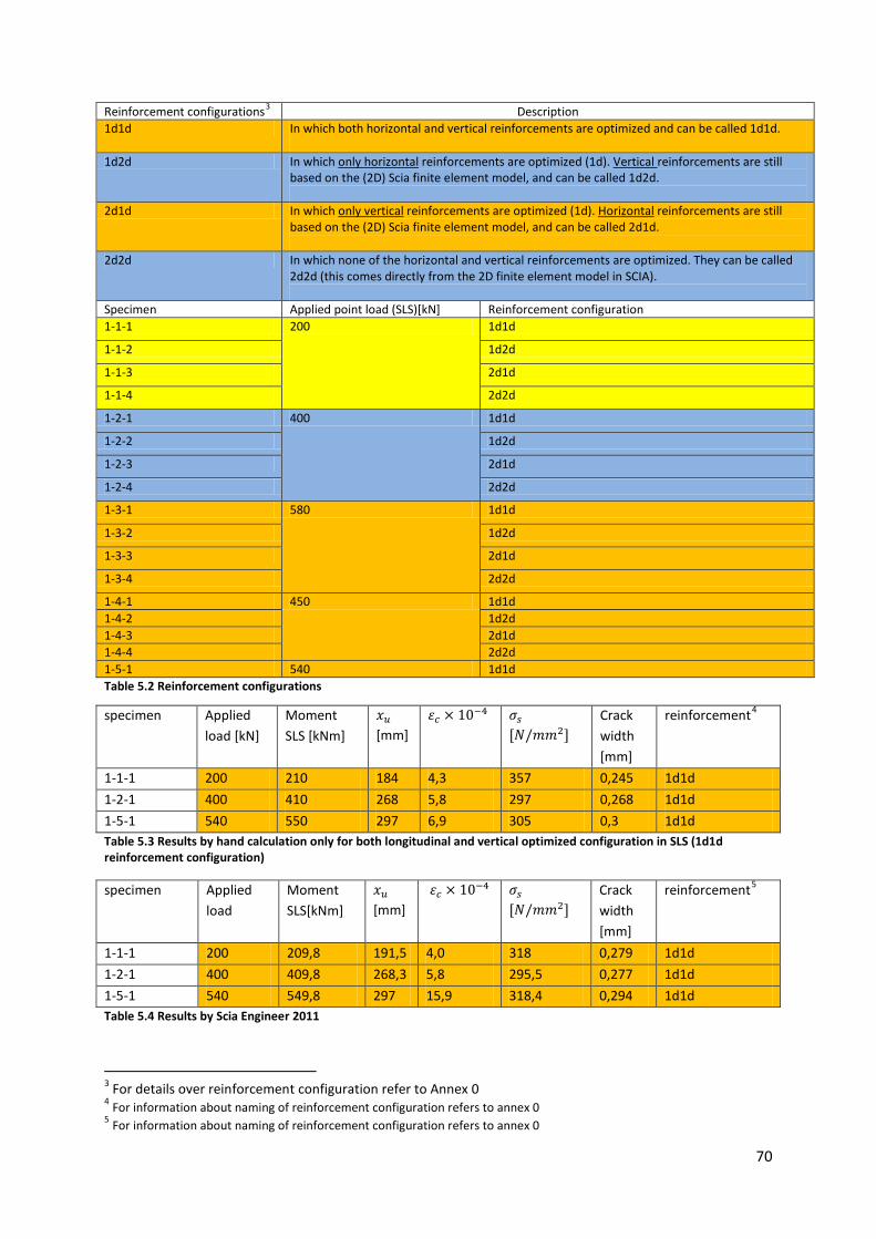
70
Reinforcement configurations3 Description 1d1d In which both horizontal and vertical reinforcements are optimized and can be called 1d1d.
1d2d In which only horizontal reinforcements are optimized (1d). Vertical reinforcements are still
based on the (2D) Scia finite element model, and can be called 1d2d.
2d1d In which only vertical reinforcements are optimized (1d). Horizontal reinforcements are still based on the (2D) Scia finite element model, and can be called 2d1d.
2d2d In which none of the horizontal and vertical reinforcements are optimized. They can be called 2d2d (this comes directly from the 2D finite element model in SCIA).
Specimen Applied point load (SLS)[kN] Reinforcement configuration 1-1-1 200 1d1d
1-1-2 1d2d
1-1-3 2d1d
1-1-4 2d2d
1-2-1 400 1d1d
1-2-2 1d2d
1-2-3 2d1d
1-2-4 2d2d
1-3-1 580 1d1d
1-3-2 1d2d
1-3-3 2d1d
1-3-4 2d2d
1-4-1 450 1d1d 1-4-2 1d2d 1-4-3 2d1d 1-4-4 2d2d 1-5-1 540 1d1d Table 5.2 Reinforcement configurations
specimen Applied load [kN]
Moment SLS [kNm]
𝑥𝑢 [mm]
𝜀𝑐 × 10−4 𝜎𝑠 [𝑁/𝑚𝑚2]
Crack width [mm]
reinforcement4
1-1-1 200 210 184 4,3 357 0,245 1d1d 1-2-1 400 410 268 5,8 297 0,268 1d1d 1-5-1 540 550 297 6,9 305 0,3 1d1d Table 5.3 Results by hand calculation only for both longitudinal and vertical optimized configuration in SLS (1d1d reinforcement configuration)
specimen Applied load
Moment SLS[kNm]
𝑥𝑢 [mm]
𝜀𝑐 × 10−4 𝜎𝑠 [𝑁/𝑚𝑚2]
Crack width [mm]
reinforcement5
1-1-1 200 209,8 191,5 4,0 318 0,279 1d1d 1-2-1 400 409,8 268,3 5,8 295,5 0,277 1d1d 1-5-1 540 549,8 297 15,9 318,4 0,294 1d1d Table 5.4 Results by Scia Engineer 2011
3 For details over reinforcement configuration refer to Annex 0 4 For information about naming of reinforcement configuration refers to annex 0 5 For information about naming of reinforcement configuration refers to annex 0

71
5.2.2.2 Maximum applicable loading GTB 2010
GTB 2010 [7] is the Dutch acronym for Graphics and Tables for Concrete. GTB has a long-standing reputation in civil engineering, since it allows for fast design calculations without using complex computer calculations. GTB 2010 is completely adapted to the new European regulations. Technological standards like NEN-206-1/NEN 8005 and Eurocode 0, 1 and 2 are incorporated in GTB 2010. In GTB 2010 cl. 5.1, the concrete properties are based on Eurocode 2.
Theory background “Moment without normal force for rectangular cross sections” [7] The tables 11.2 to 11.10 in GTB2010, which are also used to find the maximum applicable load (see the following section), are based on the following:
1
1
11
(1)(2)
(3)(4)(5)
(1) , (2) (6)
(2), (3), (4), (5) (7) ( )
(6) into (7) ( )
c u cd
s s yd
Rd s c
u
s l
ydc s u
cd
Rd yd u
ydRd yd
cd
N b x fN A fM N z N zz d xA b d
fN N x d
fM b d f d x
fM b d f d d
f
α
βρ
ραρ β
ρρ β
α
= ⋅ ⋅ ⋅= ⋅
= ⋅ = ⋅= − ⋅= ⋅ ⋅
⋅→ = → = ⋅
⋅→ = ⋅ ⋅ ⋅ ⋅ − ⋅
⋅= ⋅ ⋅ ⋅ ⋅ − ⋅ ⋅
⋅
Formulas 5.6
For cross section to carry the design moment 𝑀𝐸𝑑 via 𝑀𝐸𝑑 = 𝑀𝑅𝑑
112(8) 1 ydEd
ydcd
fM fbd f
ρρ β
α⋅
= ⋅ − ⋅ ⋅
Formula 5.7
If 𝑓𝑐𝑑 and 𝑓𝑦𝑑 are known, 𝜌𝑙 is the only unknown, and can be calculated by the following relation
Concrete strength class
≤ 𝐶50/60 𝐶55/67 𝐶70/85 𝐶90/105
𝛼 0,75 0,71 0,62 0,56 𝛽 0,39 0,37 0,35 0,34
𝑥𝑢,𝑚𝑎𝑥𝑑
for yielding of concrete rebars
0,617 0,59 0,55 0,545
Table 5.5 values for , 𝜷 and 𝒙𝒖,𝒎𝒂𝒙𝒅
based on concrete strength class
With 𝑓𝑦𝑑𝑓𝑐𝑑
= 𝑘 , b and d are in m and 𝑓𝑦𝑑 and 𝑓𝑐𝑑 in 𝑁/𝑚𝑚2 and 𝑀𝐸𝑑 in kNm the above
1 2
4(9) 1 12 1000
Ed
cd
Mf bd
α βρβ α
= − −
Formula 5.8

72
Formula (9) gives the value of 100𝑘𝜌𝑙
12
1 41 12 1000
1
cd Edu u x x
yd cd
u z z x
f Mx d x k d kf f bd
z d x z k d k k
ρ βα β α
β β
= → = → = − −
= − → = = −
Formulas 5.9
With value of 𝑘𝑠from tables 11.3 till 11.10 𝐴𝑠 can be determined:
Eds
s
MAk d
=
21
Ed Eds
s
M MkA d bdρ
= =
Formulas 5.10
With b and d in m; 𝐴𝑠 𝑚𝑚2 and 𝑀𝐸𝑑 in kNm :
6 2110
Ed Eds
s
M MkA d bdρ
= = Formulas 5.11
The tables 11.2 to 11.10 in GTB2010 [7] are based on the yielding of the reinforcement and the maximum compression zone 𝑥𝑢,𝑚𝑎𝑥 as a relation with effective height d, α and β. This value is based on the following assumptions:
• strain in the highest pressure zone of concrete is 𝜀𝑐𝑢3 • highest strain in ensile rebars is 𝜀𝑦𝑑
If there is a redistribution of forces the compression height zone should be limited.
Concrete strength class
≤ 𝐶50/60 𝐶55/67 𝐶70/85 𝐶90/105
𝛿 1
0,9 0,8 0,7
0,535 0,435 0,335 0,235
0,547 0,407 0,307 0,207
0,466 0,366 0,266 0,166
0,461 0,361 0,261 0,161
Table 5.6 Adjusted relation 𝒙𝒖,𝒎𝒂𝒙
𝒅 as a function of the degree of redistribution.
Finding the maximum applicable load
It was assumed that to find the maximum capacity of the specimens with the help of the 2D finite element model in Scia Engineer one can make use of occurring of E6 errors (concrete crushing) in Scia Engineer (see the error reference annex 3), but according to ATENA’s nonlinear models the local crushing of the concrete compression zone in some parts of the beam does not mean failure of the specimens.

73
It has been decided that the maximum applicable load should be found via the maximum allowable reinforcement ratio. According to NEN-EN 1992-1-1 art 9.2.1.1, the maximum allowable reinforcement ratio is 4%, but according to GTB 2010 [7], which is based on the practical reinforcement, 2.13 % is the maximum value for reinforcement ratio.
Problem According to Wight [4] “the reinforcement ratio is the tension steel area divided by effective area of concrete.”
Because of the complexity of the reinforcement configuration, the two ways that are used in this thesis to find the maximum applicable load are the following:
• A limit reinforcement ratio of 2.13 % based only on effective tensile reinforcements in the bottom (580 kN is found to be the maximum applicable load).
• A limit reinforcement ratio of 2.13 % that is also based on skin reinforcement (flankwapening in Dutch) with a negligible tensile force (450 kN is found to be the maximum applicable load).
Specimens which are considered in analysis Specimen Applied load [kN] Reinforcement configuration6 1-1-1 200 1d1d 1-1-2 200 1d2d 1-1-3 200 2d1d 1-1-4 200 2d2d 1-2-1 400 1d1d 1-2-2 400 1d2d 1-2-3 400 2d1d 1-2-4 400 2d2d 1-3-1 580 1d1d 1-3-2 580 1d2d 1-3-3 580 2d1d 1-3-4 580 2d2d 1-4-1 450 1d1d 1-4-2 450 1d2d 1-4-3 450 2d1d 1-4-4 450 2d2d Table 5.7 Considered specimens for capacity checks [Annex 1]
6 For the definitions of reinforcement configurations refer to Annex 0 or in 5.2.2.1 table 5.2

74
Figure 5.1 Scia Engineer analyses of strains (left) stresses (middle) and the height (right) of compression zone xu.
Cl. 7.3.2 (2), to be able to calculate minimum reinforcement areas, Eurocode gives the following formula
𝐴𝑠,𝑚𝑖𝑛𝜎𝑠 = 𝑘𝑘𝑐𝑓𝑐𝑡,𝑒𝑓𝑓𝐴𝑐𝑡 Formula 5.12 𝐴𝑐𝑡 Exactly half the area of the concrete cross section, because in the beginning before cracking
occurs, reinforcements does interact with concrete, it is just like when no reinforcement is there. So the strains at top and bottom of the cross section are the same.
𝑓𝑐𝑡,𝑒𝑓𝑓 Is the mean value of the tensile strength of the concrete effective at the time when the cracks may first be expected to occur.
𝑘𝑐 Is a coefficient which takes account of the stress distribution within the section immediately prior to cracking and of the change of the lever arm.[3]
𝜎𝑠 Is the absolute value of the maximum stress permitted in the reinforcement immediately after formation of the crack.
k Is the coefficient which allows for the effect of non-uniform self-equilibrating stresses which lead to a reduction of restraint
Cl. 7.3.3 (2) has already been discussed in previous chapters.
Cl. 7.3.3 (3) According to Eurocode, beams with a total depth of 1000 mm or more and reinforcements only in some small part of the cross-section might be helpful to avoid having cracks in the additional skin reinforcement (flankwapening). The amount and spacing of these skin reinforcements can be determined by using NEN-EN 1992-1-1 cl. 7.3.2 (2) and cl.7.3.4. The possibility of applying additional skin reinforcement can be check by using the following relations [6].
max 2
22
2
max
(1)1/ 2 1/ 2(2)
combination (1)and (2)
1/ 2
s
ss s
s u u
su
w tt t
d x d x
twd x
εε ε εε
ε
= ⋅
⋅ ⋅= → =
− −
⋅=
−
Formulas 5.13
𝑤𝑚𝑎𝑥 Maximum acceptable crack width T The crack is at its largest at about 1/2t under the natural line

75
𝜺𝒔=0,0015 Strain in cross section at the distance of 𝒅 − 𝒙𝒖 𝜺𝒔𝟐 Strain in cross section at the distance of 1/2t from neutral line 𝒙𝒖 Compression zone 𝒅 Effective height of cross section
Important Note:
Skin reinforcements translates in Dutch as ‘flankwapening’, not as ‘huidwapening’. This latter term refers to what is called ‘actual surface reinforcements’ in Eurocode.
NEN-EN 1992-1-1 cl. 9.2.4 and Annex J.1 or GTB 2010 -16.1.c surface reinforcement
The purposes of surface reinforcements are to resist spalling and to control cracks in the reinforced concrete elements. The surface reinforcements, or ‘huidwapening’ in Dutch, should consist of wire mesh or small diameter bars and it is placed outside the links. They should be used when the following reinforcement configuration is applied:
1- Rebars with diameter greater than 32 mm or 2- Bundled rebars with equivalent diameter greater than 32 mm
Figure 5.2 Example of the surface reinforcement; x is the depth of the neutral axis at ULS [3]
In this thesis the possibility of spalling and surface cracks are not considered.
Cl. 7.3.3 (4). According to Eurocode, large cracks are likely to occur in sections where sudden changes of stress are happening, for example:
• At changes of section (not applicable to this thesis) • Near concentrated loads (applicable to this thesis) • Positions where bars are curtailed (applicable to this thesis) • Areas of high bond stress, particularly at the ends of laps (applicable to this thesis)
Cl. 7.3.4 is used for calculation of crack widths.
Cl. 7.4.1 (4), (5): Deflection control is checked according to the Eurocode and all specimens pass the checks.
5.2.2.3 Detailing of reinforcement The vertical and horizontal spacing of the reinforcing bars is checked for compliance with EN-1992-1-1 cl. 8.2 (2).
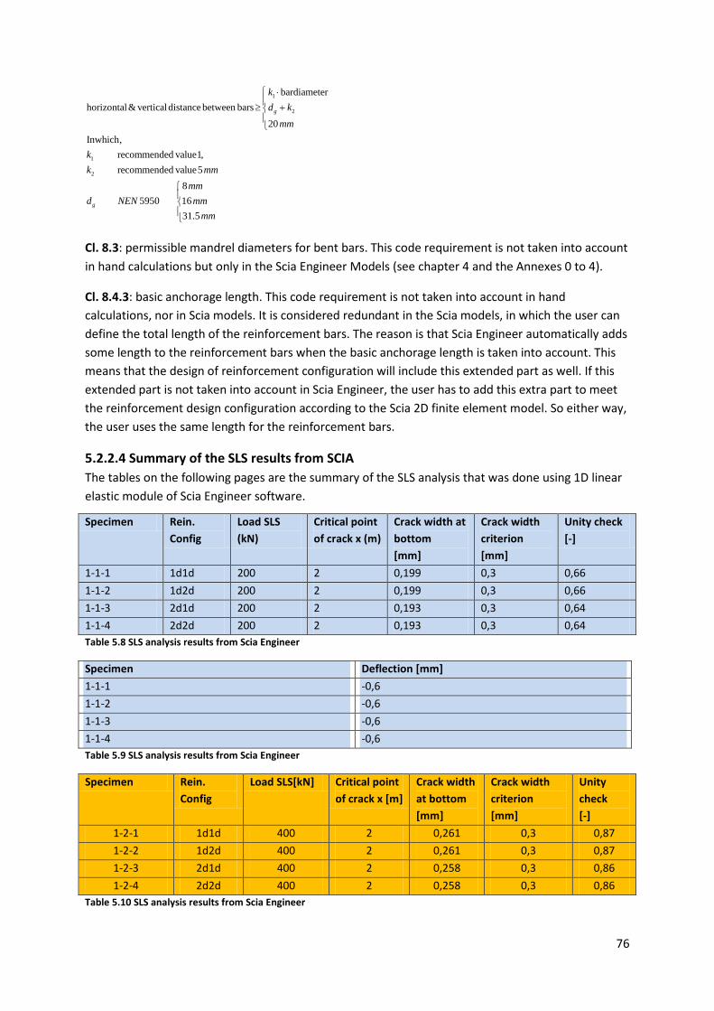
76
1
2
1
2
bardiameterhorizontal& verticaldistance between bars
20Inwhich,
recommended value1,recommended value5
85950 16
31.5
g
g
kd k
mm
kk mm
mmd NEN mm
mm
⋅≥ +
Cl. 8.3: permissible mandrel diameters for bent bars. This code requirement is not taken into account in hand calculations but only in the Scia Engineer Models (see chapter 4 and the Annexes 0 to 4).
Cl. 8.4.3: basic anchorage length. This code requirement is not taken into account in hand calculations, nor in Scia models. It is considered redundant in the Scia models, in which the user can define the total length of the reinforcement bars. The reason is that Scia Engineer automatically adds some length to the reinforcement bars when the basic anchorage length is taken into account. This means that the design of reinforcement configuration will include this extended part as well. If this extended part is not taken into account in Scia Engineer, the user has to add this extra part to meet the reinforcement design configuration according to the Scia 2D finite element model. So either way, the user uses the same length for the reinforcement bars.
5.2.2.4 Summary of the SLS results from SCIA The tables on the following pages are the summary of the SLS analysis that was done using 1D linear elastic module of Scia Engineer software.
Specimen Rein. Config
Load SLS (kN)
Critical point of crack x (m)
Crack width at bottom [mm]
Crack width criterion [mm]
Unity check [-]
1-1-1 1d1d 200 2 0,199 0,3 0,66 1-1-2 1d2d 200 2 0,199 0,3 0,66 1-1-3 2d1d 200 2 0,193 0,3 0,64 1-1-4 2d2d 200 2 0,193 0,3 0,64 Table 5.8 SLS analysis results from Scia Engineer
Specimen Deflection [mm] 1-1-1 -0,6 1-1-2 -0,6 1-1-3 -0,6 1-1-4 -0,6 Table 5.9 SLS analysis results from Scia Engineer
Specimen Rein. Config
Load SLS[kN] Critical point of crack x [m]
Crack width at bottom [mm]
Crack width criterion [mm]
Unity check [-]
1-2-1 1d1d 400 2 0,261 0,3 0,87 1-2-2 1d2d 400 2 0,261 0,3 0,87 1-2-3 2d1d 400 2 0,258 0,3 0,86 1-2-4 2d2d 400 2 0,258 0,3 0,86
Table 5.10 SLS analysis results from Scia Engineer

77
Specimen Deflection [mm] 1-2-1 -1,2 1-2-2 -1,2 1-2-3 -1,2 1-2-4 -1,2 Table 5.11 SLS analysis results from Scia Engineer
Specimen Rein. config
Load SLS[kN] Critical point of crack x [m]
Crack width at bottom [mm]
Crack width criterion [mm]
Unity check [-]
1-3-1 1d1d 580 2 0,295 0,3 0,98 1-3-2 1d2d 580 2 0,294 0,3 0,98 1-3-3 2d1d 580 2 0,287 0,3 0,96 1-3-4 2d2d 580 2 0,287 0,3 0,96 Table 5.12 SLS analysis results from Scia Engineer
Specimen Deflection [mm] 1-3-1 -1,7 1-3-2 -1,7 1-3-3 -1,7 1-3-3 -1,7 Table 5.13 SLS analysis results from Scia Engineer
Specimen Rein. config
Load SLS[kN] Critical point of crack x [m]
Crack width At bottom [mm]
Crack width criterion [mm]
Unity check [-]
1-4-1 1d1d 580 2 0,258 0,3 0,86 1-4-2 1d2d 580 2 0,265 0,3 0,88 1-4-3 2d1d 580 2 0,249 0,3 0,83 1-4-4 2d2d 580 2 0,256 0,3 0,85 Table 5.14 SLS analysis results from Scia Engineer
Specimen Deflection [mm] 1-4-1 -1,3 1-4-2 -1,3 1-4-3 -1,3 1-4-3 -1,3 Table 5.15 SLS analysis results from Scia Engineer
5.2.2.5 Brief results from PNL analysis (specimen 1-2-4) Stiffness diagram
As has already been explained, stiffness is modified in locations where cracks are occurring in the specimen. This results in a decrease of the stiffness in the middle of the span, where cracks are occurring as a result of the bending. The dimension is 𝑀𝑝𝑎 ∙ 𝑚2, from which module of elasticity of concrete can be easily derived.
At support area
𝐸𝑐𝐴𝑐 = 6801 𝑀𝑝𝑎 ∙ 𝑚2

78
𝐴𝑐 = 0,2 𝑚 ∙ 1,0 𝑚 = 0,2 𝑚2
𝐸𝑐 =6801 𝑀𝑝𝑎
0,2 𝑚2 ≈ 34000 𝑀𝑝𝑎
At middle section
𝐸𝑐𝐴𝑐 = 2866 𝑀𝑝𝑎 ∙ 𝑚2
𝐴𝑐 = 0,2 𝑚 ∙ 1,0 𝑚 = 0,2 𝑚2
𝐸𝑐 = 6801 𝑀𝑝𝑎0,2 𝑚2 ≈ 14300 𝑀𝑝𝑎
Deflection
As a direct result of decreasing stiffness of the slender beam, the deflection increases to -2,80 mm.
Figure 5.4 Deflection of the beam as predicted by PNL analysis in SLS
5.2.2.6 Conclusions and recommendations 1- In the serviceability limit state, all specimens meet the Eurocode requirements. 2- Using the 1D beam model in Scia for ULS, SLS and crack width control is fast and more
accurate. Accuracy here means that Scia is able to quickly calculate the right values of stresses and strains in the bar reinforcements. In simplified hand calculation the flawed assumption is made that in ULS all bar reinforcements are yielding. Also, finding the accurate values by hand calculation takes a lot of time.
3- For crack width control requirements, one would do wise to use the 1D model in Scia Engineer. It is more accurate and time efficient.
4- The difference between reinforcement configurations and reality (ATENA analysis) will be discussed in chapter 8.
5- There is no difference between the various reinforcement configurations in Scia Engineer. All reinforcement configurations lead to almost the same results.
6- Going by the previous point, one can conclude only on the basis of SLS results from Scia Engineer that the reinforcement configuration 1d1d is the most efficient reinforcement configuration because of the following reasons:
• Lower amount of longitudinal reinforcements • Lower amount of shear reinforcements
Figure 5.3 Results of PNL analysis in SLS of reduction of stiffness at cracked areas

79
7- Further research into the abilities of PNL analysis in 1D beam structures in Scia Engineer is needed.
5.2.3 Verification of moment and shear capacity in ULS
5.2.3.1 Introduction • Capacity check for slender beams is done by hand calculation and through Maple. • ULS checks for Slender beam specimens also is done by using Scia Engineer 2011’s 1D
element • This chapter contains the Eurocode requirements for ULS • Ultimate limit state is checked based on NEN- EN 199-1-1 cl. 6.1 • Bending for the beams is check based on NEN- EN 199-1-1 cl. 9.2 • Shear for the beams is checked based on NEN- EN 199-1-1 cl.6.2.2
5.2.3.2 Bending with or without axial force General points According to NEN-EN 1992-1-1 cl.6.1 (2), the following assumptions are made in determination of the ultimate moment resistance of reinforced concrete cross-sections:
• Plane sections remain plane. • The strain in bonded reinforcement, whether in tension or in compression, is the same as
that in the surrounding concrete. • The tensile strength of the concrete is ignored.
According to NEN-EN 1992-1-1 cl.6.1 (3), the compressive strain in the concrete should be limited to 𝜀𝑐𝑢2 or 𝜀𝑐𝑢3 depending on the stress-strain diagram that is used (NEN-EN 1992-1-1 cl. 3.1.7 and Table 3.1). The strains in the reinforcing steel should be limited to 𝜀𝑢𝑑 (where applicable).
5.2.3.3 Mean distance of reinforcement bars from bottom to the top ‘d’ Most of the specimens have multiple layers of reinforcements. To find out the ‘d’ value, one can use the following center of area formulas:
𝑌𝑐 = ∑𝐴𝑖∙𝑦𝑐,𝑖∑𝐴𝑖
Formula 5.14
𝑦𝑐,𝑖 The distance of bars with respect to a reference point
𝐴𝑖 The area of the reinforcement bars
𝑑 = ℎ − 𝑦𝑐
According to NEN-EN 1992-1-1 cl. 9.2.1.1 (1), the minimum amount of reinforcement can be calculated as following

80
,min t
2/3
0.26 but not less than 0.0013b d
3.1, 1992 1 1
0.3
ctms t
yk
ctm
ctm ck
fA b df
f Table ENf f
= ⋅ ⋅ ⋅
− −
= ⋅
Formula 5.15
NEN-EN 1992-1-1 Art 9.2.1.1 (3) According to Eurocode, there are two possible solutions for maximum possible amount of reinforcement:
(1) National annex GTB 2010- 11.5 C30/37 B500 (Graphics and tables for concrete). According to GTB, the maximal reinforcement is 2.13 % of the cross-section.
(2) ,max 0.04s cA A=
Requirements according to NEN-EN 1992-1-1 cl.9.2.1.3, are already explained in chapter 3 in reinforcement section.
5.2.3.4 Moment capacity The bilinear stress strain relation for concrete suggests that the maximum strain that can be absobed by concrete is 3 0.0035cuε = . Higher strains will cause the crushing of the concrete.
By using equilibrium formulas from the lecture notes [6] one can find the moment capacity at each cross-section of the beam elements.
Assumption:
During hand calculation, it is assumed that all reinforcement bars in ULS are yielding. The following formulas are used to find moment capacity and strains in rebars.
𝑓𝑦𝑑 = 435 𝑁/𝑚𝑚2
𝑁𝑠 = 𝐴𝑠 ∙ 𝐸𝑠 ∙ 𝜀𝑠,𝑖 Formulas 5.16
𝜀𝑠,𝑖 = �ℎ−ℎ𝑏𝑎𝑟,𝑖𝑥𝑢
− 1� ∙ 𝜀𝑐𝑢3
ℎ𝑏𝑎𝑟,𝑖 The distance between rebars and bottom edge 𝑥𝑢 The distance of concrete compressive zone (unknown) 𝜀𝑠,𝑖 Strain in steel rebars 𝜀𝑐𝑢3 ultimate concrete strain 𝑁𝑐 = 0,75 ∙ 𝑏 ∙ 𝑥𝑢 ∙ 𝑓𝑐𝑑 𝑓𝑐𝑑 design value of concrete compressive strength Cl.3.6.1(1) 𝑓𝑐𝑑 = 𝑓𝑐𝑘
𝛾𝑐
Cl.2.4.2.4(1) 𝛾𝑐 = 1,15
Equation1 𝑁𝑐 = 𝑁𝑠

81
By solving equation (1), the unknown 𝑥𝑢 can be found.
Moment capacity 𝑀𝑢 = ∑𝑁𝑠𝑦,𝑖 ∙ (𝑑𝑖 − 0,39𝑥𝑢) Formulas 5.17
𝑁𝑠𝑦,𝑖 steel bar yielding force
𝑁𝑠𝑦,𝑖 = 𝐴𝑠,𝑖 ∙ 𝑓𝑦𝑘
The assumption about the yielding of all tensile reinforcement bars can be checked with the simple expression below.
, 3( )i u
s i cuu
d xx
ε ε −= ⋅
Formula 5.18
Hand calculations are done at the following points. The results generated by the Maple software (Annex 9) are in the following tables.
1) At the middle of the beam (x=0) 2) At one point that is calculated by Scia and has a critical unity check value of about 1
The Scia Engineer results are presented in table 5.16.
Specimens Applied load[kN]
Position section x [m]
ydM Design
moment [kNm] uM Moment
capacity[kNm]
/yd uM M
[-] 1-1 200 2 272 325 0,83 1-2 400 2 532 690 0,77 1-5 540 2 714 857 0,83 Table 5.15 Hand calculations only for vertical and horizontal optimized reinforcement configuration (1d1d).
Specimens Applied load[kN]
Position section x [m]
ydM Design
moment[kNm] uM Moment
capacity[kNm]
/yd uM M
[-] 1-1 200 2 271 331 0,82 1-2 400 2 531,7 677,5 0,78 1-5 540 2 713 833 0,85 Table 5.16 Scia Engineer results
5.2.3.5 Shear capacity NEN-EN 1992-1-1 cl. 6.2.2 (1) formula (6.2.a and 6.2.b) Shear capacity for elements without shear reinforcement has been calculated, to check whether the element need shear reinforcements or not. NEN-EN 1992-1-1 art 6.2.3 (3) If shear reinforcement is needed the following formulas can be used to find out the required shear reinforcement. These relations also are explained in reference [6].
Needed 𝐴𝑠𝑤𝑠
= 𝑉𝐸𝑑𝑧𝑓𝑦𝑤𝑑𝑐𝑜𝑡𝜃
Formula 5.19
𝐴𝑠𝑤
𝑠 The area of 2 vertical shear reinforcements (loop) 𝑧 The distance between shear reinforcement loops

82
𝑓𝑦𝑤𝑑 435 𝑁/𝑚𝑚2 1 < 𝑐𝑜𝑡𝜃 < 2,5
One can use the formula above to find 𝐴𝑠𝑤 , the needed shear reinforcement. It is possible to find 𝑉𝑅𝑑, the shear resistance of the element with shear reinforcement, by using the value of the known𝐴𝑠𝑤. The value of 𝑉𝑅𝑑 can be calculated on the basis of the smaller value of the two following formulas from NEN-EN 1992-1-1 cl. 6.2.3 (3).
,
,max 1
cot
/ (cot tan )
swRd s ywd
Rd cw w cd
AV zfs
V b zv f
θ
α θ θ
=
= +
Formulas 5.20
𝐴𝑠𝑤 The cross-sectional area of the shear reinforcements s The spacing of the stirrups 𝑓𝑦𝑤𝑑 The design yield strength of the shear reinforcements 𝑣1 A strength education factor for concrete cracked in shear 𝛼𝑐𝑤 A coefficient that takes the state of the stress in the compression chord into account. As
this thesis is about reinforced concrete (not pre-stressed) the recommended value is 1.
The recommended value for 𝑣1 is 𝑣 = 0,6 �1− 𝑓𝑐𝑘250
�, but if the design stress of the shear
reinforcement is below 80% of the characteristic yield stress 𝑓𝑦𝑘 there are two possible values for 𝑣1:
𝑣1=0,6 For 𝑓𝑐𝑘 ≤ 60 𝑀𝑃𝑎
𝑣1=0,9-𝑓𝑐𝑘2
200 > 0,5 For 𝑓𝑐𝑘 ≥ 60 𝑀𝑃𝑎
In hand calculation 𝜃 = 45, 𝑐𝑜𝑡𝜃 = 1 but in the Scia Engineer1D beam model analysis 𝜃 = 40, 𝑐𝑜𝑡𝜃 = 1,192 (for Scia Engineer requirements refer to Annex 4). With bigger 𝜃, more shear reinforcement is calculated, which result in higher shear capacities.
5.2.3.6 Hand calculations Specimen Applied
load 𝑉𝐸𝑑ends [kN]
𝑉𝑅𝑑𝑐[kN] Shear reinforcement
𝑉𝑅𝑑,𝑚𝑎𝑥 [kN]
𝑉𝑅𝑑 [kN]
Unity check
1-1 200 142 83 10-300 780 199 0,7 1-2-1 400 272 99 10-200 871 272 1 1-3 540 363 93 10-100 864 491 0,7 Table 5.17
5.2.3.7 Scia calculations Specimen Applied
load 𝑉𝐸𝑑 ends [kN]
𝑉𝑅𝑑𝑐 [kN]
Shear reinforcement
𝑉𝑅𝑑,𝑚𝑎𝑥 [kN]
𝑉𝑅𝑑 [kN]
Unity check
1-1-1 200 130 78,2 10-300 811 229 0,57 1-2-1 400 260 102,2 10-200 812 318 0,82 1-5 540 351 110 10-100 801 627 0,56 Table 5.18

83
5.2.3.8 Possible failure mode in Scia In this section the possible failure mechanism in Scia Engineer 2011 is determined by simply looking at the capacity check ratios for the moment and shear forces. The most critical capacity check ratio (whether moment or shear) determines the failure mechanism.
Table 5.19 Loading process and results for specimens with applied load 200 kN
Applied Load [kN]
Specimens Reinforcement configuration8
X [m] 𝑀𝑦/𝑀𝑢 Critical point x coordinate
Vy/vrd Crack width
400 1-2-1 1d1d 0,7 0,8 All x 0,87 0,87 1-2-3 2d1d 0,7-2 0,75-0,74 All x 0,89 0,86 1-2-2 1d2d 0,7 0,8 All x 0,56 0,87 1-2-4 2d2d 0,7-2 0,75-0,74 All x 0,57 0,87
450 1d1d 0,7-2 0,9-0,84 All x 0,97 - 2d1d 0,7-2 0,84-0,83 0,7 1,02 - 1d2d 0,7-2 0,9-0,84 All x 0,63 - 2d2d 0,7-2 0,84-83 0,4 0,66 -
570 1d1d 0,7-0,2 1,1-1,02 All x 1,2 - 2d1d 0,7-2 1,06-1,04 All x 1,28 - 1d2d 0,7-2 1,13-1,06 All x 0,8 - 2d2d 0,7-2 1,06-1,04 0,4 0,82 -
Table 5.20 Loading process and results for specimens with applied load 400 kN
7 For reinforcement configuration refer to Annex 0 8 For reinforcement configuration refer to Annex 0
Applied Load [kN]
Specimens Reinforcement configuration7
X [m] 𝑀𝑦/𝑀𝑢 Critical point x coordinate
𝑉𝑦/𝑉𝑅𝑑 Crack width
200 1-1-1 1d1d 2 0,61 All x 0,59 0,66 1-1-3 2d1d 2 0,58 All x 0,6 0,64 1-1-2 1d2d 2 0,61 All x 0,5 0,66 1-1-4 2d2d 2 0,58 All x 0,5 0,64
300 1d1d 2 0,9 0,4,0,7 0,87 - 2d1d 2 0,85 All x 0,87 - 1d2d 2 0,9 All x 0,7 - 2d2d 2 0,85 All x 0,76 -
450 1d1d 0,5-2 1-1,34 All x Greater than 1,2
-
2d 1d 2 1,26 All x Greater than 1,3
-
1d2d 2-0,5 1,34-1 All x Round 1,1 - 2d2d 2 1,26 All x 1,14 -

84
Applied Load [kN]
Specimens
Rein config
Critical point x coordinate
My/muy Critical point x coordinate
Vy/vrd Crack
580 1-3-1 1d1d 2 0,85 All x 0,64 0,98 1-3-3 2d1d 2 0,84 Allx 0,65 0,96 1-3-2 1d2d 2 0,85 All x About 0,58 0,98 1-3-4 2d2d 2 0,84 Allx 0,58 0,96
650 1d1d 2 0,95 All x 0,72 2d1d 2 0,94 All x 0,7 1d2d 2 0,95 All x About 0,64 2d2d 2 0,94 All x 0,65
750 1d1d 2 1,09 Allx-near support 0,83 2d1d 2 1,08 All x-near support 0,84 1d2d 2 1,09 All x About 0,74 2d2d 2 1,08 All x 0,75
Table 5.21 Loading process and results for specimens with applied load 580 kN
Applied Load [kN]
Specimens Reinforcement configuration
Critical point x coordinate
My/muy Critical point x coordinate
Vy/vrd crack
450 1-4-1 1d1d 2 0,75 All x 0,8 0,86 1-4-3 2d1d 2 0,73 All x 0,83 0,83 1-4-2 1d2d 2 0,75 All x 0,49 0,88 1-4-4 2d2d 2 0,74 All x 0,51 0,85
Table 5.22
Specimen Rein. Config Possible failure mechanism 1-1-1
1d1d Bending
1-2-1 1-4-1
Shear
1-3-1 Bending 1-1-3 1-2-3 1-4-3
2d1d
Shear
1-3-3 Bending in the middle is governing for failure. 1-1-2 1-2-2 1-3-2 1-4-2
1d2d
Bending is governing
1-1-4 1-2-4 1-3-4 1-4-4
2d2d
Bending is governing
Table 5.23 Possible failure mechanism
From table 5.23 can recognize the possible failure mechanism in the above models. This can be compared with the results of the failure mechanisms which is found with help of ATENA in chapter 8.
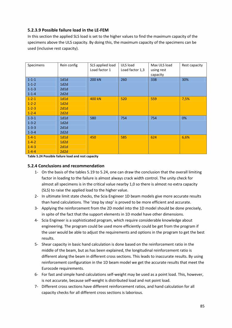
85
5.2.3.9 Possible failure load in the LE-FEM In this section the applied SLS load is set to the higher values to find the maximum capacity of the specimens above the ULS capacity. By doing this, the maximum capacity of the specimens can be used (inclusive rest capacity).
Specimens Rein config SLS applied load Load factor 1
ULS load Load factor 1,3
Max ULS load using rest capacity
Rest capacity
1-1-1 1-1-2 1-1-3 1-1-4
1d1d 1d2d 2d1d 2d2d
200 kN 260 338 30%
1-2-1 1-2-2 1-2-3 1-2-4
1d1d 1d2d 2d1d 2d2d
400 kN 520 559 7,5%
1-3-1 1-3-2 1-3-3 1-3-4
1d1d 1d2d 2d1d 2d2d
580 754 754 0%
1-4-1 1-4-2 1-4-3 1-4-4
1d1d 1d2d 2d1d 2d2d
450 585 624 6,6%
Table 5.24 Possible failure load and rest capacity
5.2.4 Conclusions and recommendation 1- On the basis of the tables 5.19 to 5.24, one can draw the conclusion that the overall limiting
factor in loading to the failure is almost always crack width control. The unity check for almost all specimens is in the critical value nearby 1,0 so there is almost no extra capacity (SLS) to raise the applied load to the higher value.
2- In ultimate limit state checks, the Scia Engineer 1D beam models give more accurate results than hand calculations. The ‘step by step’ is proved to be more efficient and accurate.
3- Applying the reinforcement from the 2D model into the 1D model should be done precisely, in spite of the fact that the support elements in 1D model have other dimensions.
4- Scia Engineer is a sophisticated program, which require considerable knowledge about engineering. The program could be used more efficiently could be get from the program if the user would be able to adjust the requirements and options in the program to get the best results.
5- Shear capacity in basic hand calculation is done based on the reinforcement ratio in the middle of the beam, but as has been explained, the longitudinal reinforcement ratio is different along the beam in different cross sections. This leads to inaccurate results. By using reinforcement configuration in the 1D beam model we get the accurate results that meet the Eurocode requirements.
6- For fast and simple hand calculations self-weight may be used as a point load. This, however, is not accurate, because self-weight is distributed load and not point load.
7- Different cross sections have different reinforcement ratios, and hand calculation for all capacity checks for all different cross sections is laborious.

86
5.2.5 Disadvantages of Scia Engineer • The user must have a good computer to be able to run the 2D finite element model in
fine mesh of 10 mm. • The Scia Engineer 2D finite element model is not capable of giving the exact failure load.
This means that it is not possible to determine the maximum capacity of the specimen on the basis of the Scia Engineer 2D model.
• In theory, if the concrete crushing occurs at the compression zone, the element is locally failing and all bottom reinforcements are already yielding. But in reality the local crushing of the concrete means neither failure nor yielding of all bottom reinforcements. This will be also elaborated with the help of ATENA (nonlinear analysis) in chapter 8 and annex 8.
• Mesh dependency in the results of the Scia Engineer’s finite element model analysis is observed. This mesh dependency makes it impossible to determine failure mode by looking at the E6 error (concrete crushing error (Annex 4)) in the finite element mesh.
References
[1] “Theory Design of concrete structures” Scia Engineer 2008
[2] Master thesis “Design of walls with linear elastic finite element methods” Marc Romans 2010, TU Delft , concrete structures
[3] Eurocode 2: Design of concrete structures Part 1-1: General rules and rules for buildings NEN EN 1992-1-1 [4] Book “Reinforced concrete” James K. Wight and James G. MacGregor, Fifth Edition
[5] Building structures 2 CIE4148, TU Delft , lecture book.
[6] CIE 2052 “Gewapend Beton” Civil Engineering, TU Delft ,March 2010 Prof.dr.ir. –Ing.h.c. J.C. Walraven
[7] GTB 2010, Graphics and Tables for Concrete, based on Eurocode, 2010

87
Chapter 6 Non-Linear Finite Element Analysis: Principles, Slender and Deep beams
6.1 Summary In this chapter the principles of nonlinear finite element analysis will be explained. The order of the subchapters is the same as the order of the modeling in the NL-FEM software package ATENA. In this chapter the instructions are introduced to ease the decision-making in the modeling process. All model parameters that are needed to make a model are explained in detail and clarified with the help of references to annexes. The chapter closes with a summary of the important material properties and some recommendations are represented.
6.2 Introduction Nonlinear analysis according to Eurocode
As was mentioned in the previous chapters, non-linear finite element analysis is an essential part of this thesis. With the help of nonlinear analysis one can simulate the real behavior of concrete elements. The aim of non-linear analysis in this thesis is to compare different reinforcement configurations which are determined by Scia Engineer 2011 for SLS and ULS with real behavior of the reinforced concrete elements. These results are going to be used to determine whether one can use the Scia Engineer 2D finite element module to reinforce different concrete elements in a reliable manner. The non-linear finite element software that is used during this thesis is ATENA 2D version 4.3.1.0. Other researchers may have used the name SBETA, the older name of ATENA, in their theses. The name “SBETA” is an abbreviation of the analysis of reinforced concrete in German: (StahlBETonAnalyse) [1].
Note:
• The principles of nonlinear finite element analysis are given in this chapter. • The parameters in this chapter are presented in an order that corresponds with the modeling
procedure in the ATENA software. • Material properties are made mostly the same as in chapter 3 (Eurocode NEN-EN 1992-1-1). • To enable the reader to follow the theory as well as the ATENA program, figures from the
ATENA interface are included after each theoretical section. • For reinforcement configurations and naming, see annex 0. • For details on making the ATENA model, see annex 6.
Some related articles from Eurocode about nonlinearity are collected which are the basics for non-linear analysis:
NEN-EN 1992-1-1 cl.3.1.5, NEN-EN 1992-1-1 cl.5.7, NEN-EN-1992-2+C1 cl.5.7
6.3 Model Parameters and Specifications in Nonlinear Finite Element Analysis
6.3.1 Concrete constitutive model SBETA (CCSbetaMaterial) In this thesis the material model SBETA is going to be used [4], [5], [6]. The SBETA constitutive model includes 20 material parameters. If the parameters are not known, they can be automatically generated ATENA. The automatic generation in ATENA needs only one input, which is the cubic

88
strength of the concrete. The formulas from which all other parameters can be derived are all taken from CEB-FIP model code 90 [7]. Figure 6.1 shows an example of the SBETA material model configuration in ATENA.
Figure 6.1 SBETA material interface
Concept of Material Model SBETA
The material model SBETA includes the following effects of concrete behavior:
• Non-linear behavior in compression, including hardening and softening;
• Fracture of concrete in tension based on the nonlinear fracture mechanics;
• Biaxial strength failure criterion; • Reduction of compressive strength
after cracking; • Tension stiffening effect; • Reduction of the shear stiffness after
cracking (variable shear retention); • Two crack models: fixed crack
direction and rotated crack direction;
6.3.1.1 Stress-strain relations for concrete Equivalent uniaxial law
In the figure below the nonlinear behavior of the concrete in the biaxial stress state is shown by
means of the effective stress (in most cases a principal stress) 𝜎𝑐𝑒𝑓 and the equivalent uniaxial
strain 𝜀𝑒𝑓.
ef ci
ciEσε =
Formula 6.1
Table 6.1 Default formulas of material parameters according to CEB-FIP Model Code 90 [7]

89
Figure 6.2 Uniaxial stress-strain law [4]
Figure 6.3 SBETA material properties in ATENA
The equivalent uniaxial strain can be derived by the stress σci in a uniaxial test with elasticity modules Eci associated with the direction i. In the stress-strain diagram in figures 6.1 and 6.3 one can recognize four different material state numbers which correspond to four different phases of the stress-strain state.
Material state number 1
Tension before cracking (un-cracked)
The behavior of the concrete before cracking in the tension zone is assumed to be linear elastic, and
the slope is equal to the initial module of elasticity of the concrete. In figure 6.2 𝑓𝑡′𝑒𝑓 is the effective
tensile strength derived from the biaxial failure function:
𝜎𝑐𝑒𝑓 = 𝐸𝑐𝜀𝑒𝑞 , 0 ≤ 𝜎𝑐 ≤ 𝑓𝑡
′𝑒𝑓
Formula 6.2
Material state number 2
Tension after cracking (process zone)
Due to a bridging effect, crack formation occurs in the process zone with decreasing tensile stress on a crack face and after process zone crack opening continues without the stress. Crack width can be calculated with the following formula:
𝑤 = 𝜀𝑐𝑟𝐿′𝑡 Formula 6.3

90
𝜀𝑐𝑟 The crack opening strain equal to the crack direction in the cracked state after the complete stress release.
There are two types of formulations which can be used for crack opening:
• A fictitious crack model based on a crack opening law and fracture energy. This is a proper model for crack developments in concrete. This is the model that is used in this thesis.
• Another formulation, which is not suitable for normal case of crack developments in concrete, is ‘A stress-strain relation in a material point’.
Figure 6.4 Crack opening law
Material state number 3
Compression before peak stress
Figure 6.5 Compression strain
The CEB/FIP model code 90 recommends the following formula for the ascending part of the diagram:
Figure 6.6 Compressive stress-strain diagram
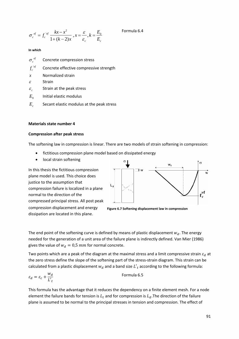
91
2' 0, ,
1 ( 2)ef ef
c cc c
Ekx xf x kk x E
εσε
−= = =
+ −
Formula 6.4
In which
efcσ Concrete compression stress 'ef
cf Concrete effective compressive strength
x Normalized strain ε Strain
cε Strain at the peak stress
0E Initial elastic modulus
cE Secant elastic modulus at the peak stress
Materials state number 4
Compression after peak stress
The softening law in compression is linear. There are two models of strain softening in compression:
• fictitious compression plane model based on dissipated energy • local strain softening
In this thesis the fictitious compression plane model is used. This choice does justice to the assumption that compression failure is localized in a plane normal to the direction of the compressed principal stress. All post peak compression displacement and energy dissipation are located in this plane.
The end point of the softening curve is defined by means of plastic displacement 𝑤𝑑. The energy needed for the generation of a unit area of the failure plane is indirectly defined. Van Mier (1986) gives the value of 𝑤𝑑 = 0,5 𝑚𝑚 for normal concrete.
Two points which are a peak of the diagram at the maximal stress and a limit compressive strain 𝜀𝑑 at the zero stress define the slope of the softening part of the stress-strain diagram. This strain can be calculated from a plastic displacement 𝑤𝑑 and a band size 𝐿′𝑡 according to the following formula:
𝜀𝑑 = 𝜀𝑐 +𝑤𝑑𝐿′𝑡
Formula 6.5
This formula has the advantage that it reduces the dependency on a finite element mesh. For a node element the failure bands for tension is 𝐿𝑡 and for compression is 𝐿𝑑.The direction of the failure plane is assumed to be normal to the principal stresses in tension and compression. The effect of
Figure 6.7 Softening displacement law in compression
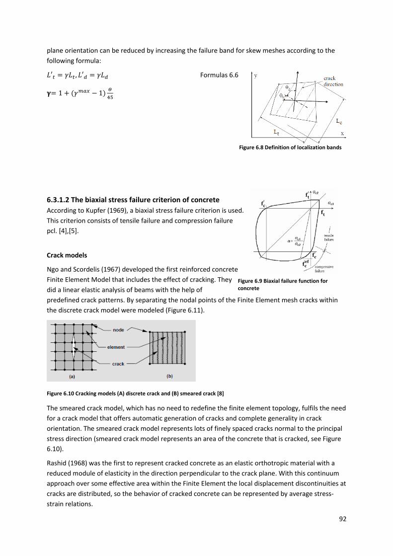
92
plane orientation can be reduced by increasing the failure band for skew meshes according to the following formula:
𝐿′𝑡 = 𝛾𝐿𝑡 ,𝐿′𝑑 = 𝛾𝐿𝑑
𝛄= 1 + (𝛾𝑚𝑎𝑥 − 1) 𝛩45
Formulas 6.6
6.3.1.2 The biaxial stress failure criterion of concrete According to Kupfer (1969), a biaxial stress failure criterion is used. This criterion consists of tensile failure and compression failure pcl. [4],[5].
Crack models
Ngo and Scordelis (1967) developed the first reinforced concrete Finite Element Model that includes the effect of cracking. They did a linear elastic analysis of beams with the help of predefined crack patterns. By separating the nodal points of the Finite Element mesh cracks within the discrete crack model were modeled (Figure 6.11).
Figure 6.10 Cracking models (A) discrete crack and (B) smeared crack [8] The smeared crack model, which has no need to redefine the finite element topology, fulfils the need for a crack model that offers automatic generation of cracks and complete generality in crack orientation. The smeared crack model represents lots of finely spaced cracks normal to the principal stress direction (smeared crack model represents an area of the concrete that is cracked, see Figure 6.10).
Rashid (1968) was the first to represent cracked concrete as an elastic orthotropic material with a reduced module of elasticity in the direction perpendicular to the crack plane. With this continuum approach over some effective area within the Finite Element the local displacement discontinuities at cracks are distributed, so the behavior of cracked concrete can be represented by average stress-strain relations.
Figure 6.9 Biaxial failure function for concrete
Figure 6.8 Definition of localization bands

93
The model SBETA material model in ATENA is using the smeared crack approach to model the cracks. There are two options available within the smeared approach: the fixed crack model and the rotated crack model. The following points apply to both models:
• A crack occurs when the principal stress exceeds the tensile strength. • It is assumed that the cracks are uniformly distributed within the material volume.
In this thesis a fixed crack model is being used. In the fixed crack model the crack direction is given by the principal stress direction at the moment of the crack initiation. This direction does not change during further loading and represents the material axis of the orthotropy. As a general case principle stress directions do not need to be coincide with the axis of the orthotropy, as it can rotate during the loading process. This assumption produces a shear stress in crack surface. In order to prevent the effect of this artificially generated shear stress a shear retention factor is introduced as a reduction coefficient [8], [9], [4, [5], [10].
Figure 6.11 SBETA material model properties in ATENA software (left) and fixed crack model “Stress and strain state” (right)
6.3.2 Steel plates
6.3.2.1 Supports and loading points As was mentioned in chapter 3, an easy way to avoid singularities is using steel plates with a thickness of 50 mm at the position of applied load and pin supports (at the two ends of the slender beam). To get a similar situation as in the linear elastic method, the width of the plates and supports are the same as the width of the beam.
6.3.2.2 Stress-strain relationship (steel plate) The behavior of steel plats considered to be perfectly elastic (see Figure 6.14).
Figure 6.12 ATENA interface about the steel plate material property.
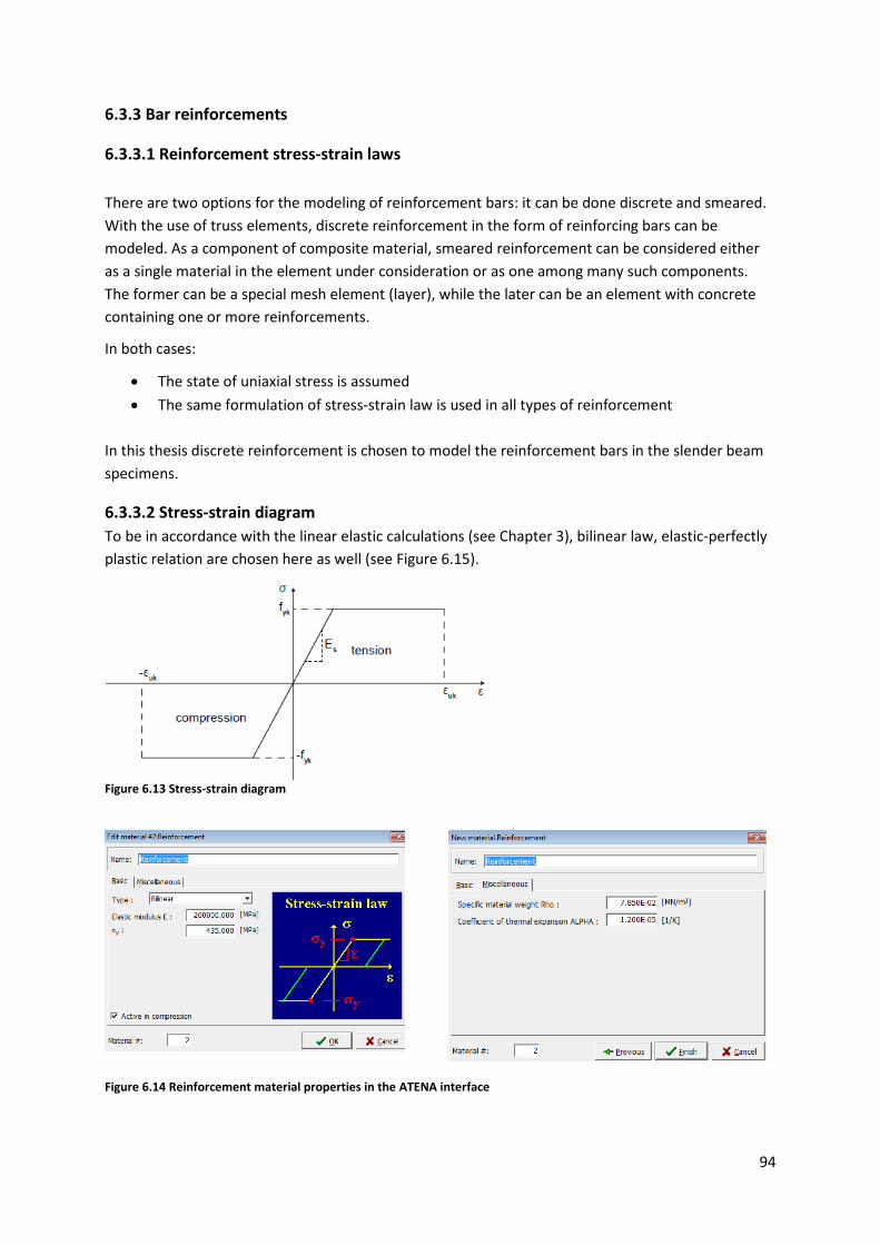
94
6.3.3 Bar reinforcements
6.3.3.1 Reinforcement stress-strain laws There are two options for the modeling of reinforcement bars: it can be done discrete and smeared. With the use of truss elements, discrete reinforcement in the form of reinforcing bars can be modeled. As a component of composite material, smeared reinforcement can be considered either as a single material in the element under consideration or as one among many such components. The former can be a special mesh element (layer), while the later can be an element with concrete containing one or more reinforcements.
In both cases:
• The state of uniaxial stress is assumed • The same formulation of stress-strain law is used in all types of reinforcement
In this thesis discrete reinforcement is chosen to model the reinforcement bars in the slender beam specimens.
6.3.3.2 Stress-strain diagram To be in accordance with the linear elastic calculations (see Chapter 3), bilinear law, elastic-perfectly plastic relation are chosen here as well (see Figure 6.15).
Figure 6.13 Stress-strain diagram
Figure 6.14 Reinforcement material properties in the ATENA interface

95
6.3.3.3 Reinforcement bond models Bond behavior The interaction between reinforcing steel and surrounding concrete is called ‘bond’. Three different phenomena cause a transformation of force from steel to concrete:
• Chemical adhesion between mortar paste and the bar surface • Friction and wedging of small particles between the reinforcements and the concrete • Mechanical interaction between concrete and steel reinforcements
Even though there is some mechanical interlocking introduced by the roughness of the bar surface, bond of plain bars is the result of the first two mechanisms just mentioned. Due to the fact that most of the steel force is transferred through the lugs to concrete, deformed bars have better bond than plain bars.
The effect of friction and chemical adhesion forces cannot be ignored, and has a tendency to decrease as the reinforcing bars start to slip. Since change in the steel force along the length causes bond stresses in reinforced concrete members, the effect of bond becomes more important at end anchorages of reinforcing bars and nearby cracks.
Figure 6.15 Tri-linear bond stress-slip models [9]
Complete compatibility of strains between reinforcement bars and concrete in simplified analysis of reinforced concrete structures is usually assumed, which implies perfect bond. However, this assumption is only realistic in regions where the stress transfer between the two components is negligible. In other cases, bond stress is related to the relative displacement between reinforcing steel and concrete, especially in regions of high transfer of stresses along the interface between reinforcing steel and surrounding concrete (such as near cracks).
In reality bond slip, which is the relative displacement between steel and concrete, is caused by strain conflict between reinforcing steel and concrete near cracks and the crack propagation. The bond-slip relationship is the basic property of the reinforcement bond model. Bond strength bτ is
defined by this relationship, and depends on the value of the current slip between the reinforcement and the surrounding concrete. There are three predefined bond-slip models in ATEBA:
• According to the CEB-FIB model code 1990 [7] • The slip law by Bigaj
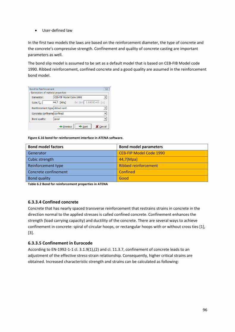
96
• User-defined law In the first two models the laws are based on the reinforcement diameter, the type of concrete and the concrete’s compressive strength. Confinement and quality of concrete casting are important parameters as well.
The bond slip model is assumed to be set as a default model that is based on CEB-FIB Model code 1990. Ribbed reinforcement, confined concrete and a good quality are assumed in the reinforcement bond model.
Figure 6.16 bond for reinforcement interface in ATENA software.
Bond model factors Bond model parameters Generator CEB-FIP Model Code 1990 Cubic strength 44,7[Mpa] Reinforcement type Ribbed reinforcement Concrete confinement Confined Bond quality Good Table 6.2 Bond for reinforcement properties in ATENA
6.3.3.4 Confined concrete Concrete that has nearly spaced transverse reinforcement that restrains strains in concrete in the direction normal to the applied stresses is called confined concrete. Confinement enhances the strength (load carrying capacity) and ductility of the concrete. There are several ways to achieve confinement in concrete: spiral of circular hoops, or rectangular hoops with or without cross ties [1], [3].
6.3.3.5 Confinement in Eurocode According to EN-1992-1-1 cl. 3.1.9(1),(2) and cl. 11.3.7, confinement of concrete leads to an adjustment of the effective stress-strain relationship. Consequently, higher critical strains are obtained. Increased characteristic strength and strains can be calculated as following:

97
, 2 2
, 2 2
22, 2 ,
2, 2 2
(1,000 5,0 / ) 0,05(1,125 2,5 / ) 0,05
( / )0,2 /
ck c ck ck ck
ck c ck ck ck
c c c ck c ck
cu c cu ck
f f f for ff f f for f
f ff
σ σ
σ σ
ε ε
ε ε σ
= + ≤
= + ≥
=
= +
Formulas 6.7
In these formulas 𝜎2 = 𝜎3 is the effective lateral compressive stress at the ULS due to confinement and 𝜀𝑐2 and 𝜀𝑐𝑢2 follow from NEN-EN 1992-1-1, table 3.1.
Figure 6.17 Stress-strain relationships for confined concrete (EN-1992-1-1 Figure 3.6)
Figure 6.18 Confining stress provided by different arrangements of transverse reinforcement [11]
6.3.3.6 Confinement further in Eurocode Confinement has also influence on anchorage and laps (EN-1992-1-1 cl. 6.6 and 8.4.4). According to EN-1992-1-1, cl. 7.2, in the absence of other measurements, such as an increase in the cover to reinforcement in the compressive zone or confinement by transverse reinforcement, it may be appropriate to limit the compressive stress to a specific value in areas exposed to environments of exposure classes XD, XF and XS [2].
Figure 6.19 Slip and bond stresses in ATENA interface (left) and bond slip law by CEB-FIP model code 1990 (right)

98
6.3.4 Interface element To model a contact between two surfaces the interface elements are used and it is defined by two lines on the opposite side of interface. These lines of interface elements have the same position and are separated by small distance which has nonzero thickness (see Figure 6.20). The interface elements have two states:
• Open (no interaction of the contact sides) • Closed (full interaction of the contact sides)
Figure 6.20 Interface element in ATENA
Figure 6.21 2D interface material properties in ATENA
6.4 Summary of Material Properties in ATENA Concrete properties ATENA E [Mpa] 3,548E+4 Poisson coefficient 0,2 Specific weight 2500 Tensile strength [Mpa] Ft=3,023 Compressive strength [Mpa] Fc=-38 Cubic strength 44,7 Specific fracture energy 7,557E-05 Type of tension softening Exponential Crack model Fixed Reduction of compressive strength due to cracks 0,8 Compressive strain at compressive strength in the uniaxial compressive test
-2,142E-03
Type of compressive softening Crush band Critical compressive displacement 𝑊𝑑 -5.0E-04 Shear retention factor Variable Tension –compression interaction Linear Coefficient of thermal expansion 1,20E-05 Table 6.3 Concrete properties
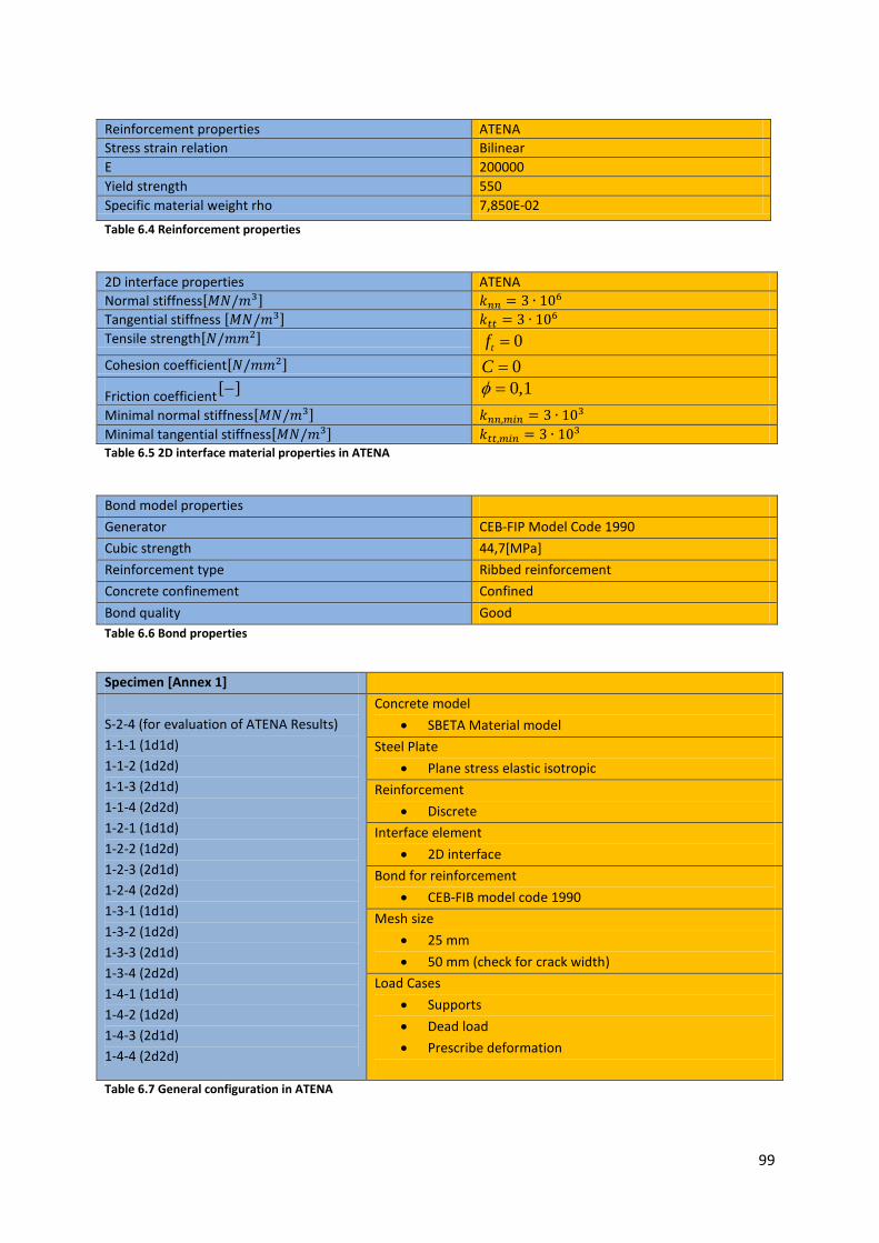
99
Reinforcement properties ATENA Stress strain relation Bilinear E 200000 Yield strength 550 Specific material weight rho 7,850E-02
Table 6.4 Reinforcement properties
2D interface properties ATENA Normal stiffness[𝑀𝑁/𝑚3] 𝑘𝑛𝑛 = 3 ∙ 106 Tangential stiffness [𝑀𝑁/𝑚3] 𝑘𝑡𝑡 = 3 ∙ 106 Tensile strength[𝑁/𝑚𝑚2] 0tf = Cohesion coefficient[𝑁/𝑚𝑚2] 0C =
Friction coefficient[ ]− 0,1φ = Minimal normal stiffness[𝑀𝑁/𝑚3] 𝑘𝑛𝑛,𝑚𝑖𝑛 = 3 ∙ 103 Minimal tangential stiffness[𝑀𝑁/𝑚3] 𝑘𝑡𝑡,𝑚𝑖𝑛 = 3 ∙ 103 Table 6.5 2D interface material properties in ATENA
Bond model properties Generator CEB-FIP Model Code 1990 Cubic strength 44,7[MPa] Reinforcement type Ribbed reinforcement Concrete confinement Confined Bond quality Good Table 6.6 Bond properties
Specimen [Annex 1] S-2-4 (for evaluation of ATENA Results) 1-1-1 (1d1d) 1-1-2 (1d2d) 1-1-3 (2d1d) 1-1-4 (2d2d) 1-2-1 (1d1d) 1-2-2 (1d2d) 1-2-3 (2d1d) 1-2-4 (2d2d) 1-3-1 (1d1d) 1-3-2 (1d2d) 1-3-3 (2d1d) 1-3-4 (2d2d) 1-4-1 (1d1d) 1-4-2 (1d2d) 1-4-3 (2d1d) 1-4-4 (2d2d)
Concrete model • SBETA Material model
Steel Plate • Plane stress elastic isotropic
Reinforcement • Discrete
Interface element • 2D interface
Bond for reinforcement • CEB-FIB model code 1990
Mesh size • 25 mm • 50 mm (check for crack width)
Load Cases • Supports • Dead load • Prescribe deformation
Table 6.7 General configuration in ATENA

100
Reinforcement configurations
(More detail [Annex 0])
• Longitudinal and vertical reinforcements according to the optimized configurations in beam model in Scia.(1d1d)
• Longitudinal reinforcement based on the beam model in Scia l and vertical reinforcement based on the 2D finite element model in Scia.(1d2d)
• Longitudinal reinforcement based on 2D Scia model and vertical reinforcement based on practical optimized reinforcement according to beam model in Scia.(2d1d)
• Longitudinal and vertical reinforcements according to 2D Scia finite element model (2d2d)
Table 6.8 Explanation about different naming of reinforcement configuration
6.5 Recommendations • Assessments of different possible constitutive models in ATENA are possible. It is important
to know that some constitutive models are more complex. Also, having a good computer is crucial. These models are newer models and have lower mesh dependencies. These other possible constitutive models are 3D NonlinCementitious 2 and 3D NonlinCementitious 3.
• Investigation about the influence of type of reinforcements smeared in comparison with discreet.
• Investigation about the support dimensions of the slender beam elements. • Investigation about the differences in results between fixed and rotated crack model. • Investigation about nonlinear analysis method which is done with ATENA
References
[1] STRENGTH ENHANCEMENT IN CONCRETE CONFINED BY SPIRALS U, Department of Civil Engineering, University of Moratuwa, U. Kaneswaran, 2011
[2] Eurocode 2: Design of concrete structures Part 1-1: General rules and rules for
buildings NEN-EN-1992-1-1
[3] “Theoretical Stress-Strain Model for Confined Concrete”, J.B. Mander
[4] ATENA Program documentation part 1 [5] ATENA program documentation part 4-1 tutorial for ATENA 2D.
[6] ATENA on the web http://www.cervenka.cz/products/atena/documentation/
[7] CEB-FIP model code 90
[8] Report “Finite element Analysis of reinforced concrete structures under Monotonic Loads” H.G. Kwak and Filip C. Flippou, Civil Engineering, University of California, November 1990
[9] “Non-Linear Finite Element Analysis of Shear Critical Reinforced Concrete Beams”, Thijs Claus

101
[10] “EXPERIMENTAL AND ANALYTICAL STUDY ON RC DEEP BEAM BEHAVIOR UNDER MONOTONIC LOAD” Mohammad Reza SALAMY, Hiroshi Kobayashi and Shigeki Unjoh.

102
Chapter 7 ATENA vs Laboratory Test
7.1 Summary In this chapter it will be examined whether the NL-FEM software package (ATENA) is reliable enough to act as a reference point for this thesis? A comparison is made between ATENA and a laboratory test. The conclusion is that ATENA can simulate the behavior of the structure correctly. Building on this conclusion, in the next chapter different models in Scia Engineer will be compared to the real behavior of the structure (ATENA model).
7. 2 Introduction It is important to note that the nonlinear analysis that is going to be used in this thesis is properly able to simulate reality. In this thesis the ATENA results have been validated with the help of the results of the experiment carried out by Van Hulten in the Stevin Laboratory at TU-Delft [2]. Melvin Asin [3] also did experiments regarding the continuous deep beams. More specifically, he did nonlinear analysis using SBETA (ATENA) software. He concluded that the non-linear analysis results (ATENA) can be used to complement experiments (see Chapter 1). The laboratory test is based on specimen S-2-4 as used by Romans [1].
7.3 ATENA vs Laboratory Test Before the ATENA analysis of the specimens, first a comparison was made between ATENA results and the laboratory test. Van Hulten [2] did laboratory tests on the specimen S-2-4 as used by Romans [1]. The aim of this chapter is to qualitatively compare the overall behavior of the specimen during the test and during the loads steps in ATENA.
• For details about the test setup, see Van Hulten’s thesis [2]. • The exact ATENA model is not available from Van Hulten’s work, so a new ATENA model is
made for this validation process. This model is based on the known reinforcement configuration from Van Hulten [2].
• As has already been mentioned, Van Hulten derived his reinforcement design from Romans’ [1] work. Figure 7.1 shows the reinforcement configuration.
Figure 7.1 Reinforcement configurations [1], [2]

103
For the sake of consistency and accuracy, the 2D model (see Figure 7.1) is also made in Scia Engineer 2011. The result of the Scia Engineer calculations leads to the conclusion that Scia Engineer still needs reinforcement bars in the 2D finite element model. This suggests that reinforcement configuration, which was made by Romans [1] in 2010, is not able to satisfy the required amount of reinforcements based on Scia Engineer’s 2D finite element 2011 calculations. Possible explanations for this difference in results include the different version of Scia Engineer and the different options in Scia Engineer that were used by Romans.
• The abovementioned deviation has no influence on the validation procedure, because the validation process is actually a comparison between ATENA and laboratory results, not between ATENA and Scia Engineer results.
• This thesis is focused on the overall behavior of the specific specimen in ATENA and in laboratory. Some factors which are important in the validation process, and any flaws could result in inaccuracy. These factors include:
a) The test setup b) The exact reinforcement configurations c) Detailed information about the ATENA model this laboratory test is based on d) Detailed results from Laboratory test (SLS and ULS)
7.4 Behavior during Laboratory Test
Load[kN]
Laboratory ATENA
250
300

104
400
500
700
800
900
Figure 7.2 Laboratory and ATENA specimens during loading phase
7.5 Validation Process Van Hulten used several test cubes to determine concrete properties in the Stevin Laboratory at TU Delft. The procedure for determining compressive strength was based on NEN-EN 12390-3[7]. Following NEN-EN 12390-1, the cube’s dimensions were set at 150 mm. The procedure from NEN-EN 12390-6 [8] was followed the tensile strength.
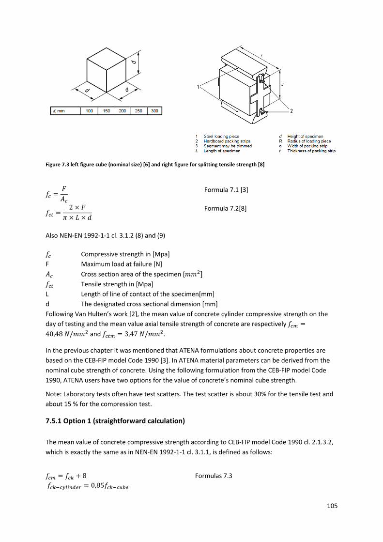
105
Figure 7.3 left figure cube (nominal size) [6] and right figure for splitting tensile strength [8]
𝑓𝑐 =𝐹𝐴𝑐
Formula 7.1 [3]
𝑓𝑐𝑡 =2 × 𝐹
𝜋 × 𝐿 × 𝑑
Also NEN-EN 1992-1-1 cl. 3.1.2 (8) and (9)
Formula 7.2[8]
𝑓𝑐 Compressive strength in [Mpa] F Maximum load at failure [N] 𝐴𝑐 Cross section area of the specimen [𝑚𝑚2] 𝑓𝑐𝑡 Tensile strength in [Mpa] L Length of line of contact of the specimen[mm] d The designated cross sectional dimension [mm] Following Van Hulten’s work [2], the mean value of concrete cylinder compressive strength on the day of testing and the mean value axial tensile strength of concrete are respectively 𝑓𝑐𝑚 =40,48 𝑁/𝑚𝑚2 and 𝑓𝑐𝑡𝑚 = 3,47 𝑁/𝑚𝑚2.
In the previous chapter it was mentioned that ATENA formulations about concrete properties are based on the CEB-FIP model Code 1990 [3]. In ATENA material parameters can be derived from the nominal cube strength of concrete. Using the following formulation from the CEB-FIP model Code 1990, ATENA users have two options for the value of concrete’s nominal cube strength.
Note: Laboratory tests often have test scatters. The test scatter is about 30% for the tensile test and about 15 % for the compression test.
7.5.1 Option 1 (straightforward calculation) The mean value of concrete compressive strength according to CEB-FIP model Code 1990 cl. 2.1.3.2, which is exactly the same as in NEN-EN 1992-1-1 cl. 3.1.1, is defined as follows:
𝑓𝑐𝑚 = 𝑓𝑐𝑘 + 8 𝑓𝑐𝑘−𝑐𝑦𝑙𝑖𝑛𝑑𝑒𝑟 = 0,85𝑓𝑐𝑘−𝑐𝑢𝑏𝑒
Formulas 7.3

106
In ATENA the input parameter for concrete is f_cu or fck−cube , as can be found above in the formulas for Option 1.
Note: The mean concrete compressive strength from the laboratory test is fcm = 40,48 N/mm2, for accuracy in the results between ATENA and laboratory this mean value from laboratory should be equal to the characteristic cylinder strength of concrete fck−cylinder or f′c (in ATENA formulation).
Using mean value of concrete compressive strength fcm = 40,48 N/mm2 into the following formula from ATENA formulation:
𝑓′𝑐 = −0,85 𝑓′𝑐𝑢 Formula 7.4
Formula 7.4 is identical to 𝑓𝑐𝑘−𝑐𝑦𝑙𝑖𝑛𝑑𝑒𝑟 = 0,85𝑓𝑐𝑘−𝑐𝑢𝑏𝑒 from CEB-FIP model Code 1990 and Eurocode. By using formulas 7.3 and 7.4 one can find the correct input ATENA parameter, which is: 𝑓′𝑐𝑢 = 𝑓_𝑐𝑢 = −47,6 𝑁/𝑚𝑚2. The tensile strength of steel reinforcement 𝜎𝑦= 550𝑁/𝑚𝑚2.
7.5.2 Option 2 (reverse calculation) The mean value of the axial tensile strength of concrete according to CEB-FIP model Code 1990 cl.2.1.3.3.1 which is identical to NEN-EN 1992-1-1 Table 3.1 is defined as follows:
CEB-FIP model Code 1990
𝑓𝑐𝑡𝑚 = 𝑓𝑐𝑡𝑘0,𝑚 �𝑓𝑐𝑘𝑓𝑐𝑘0
�2/3
,𝑓𝑐𝑡𝑘0,𝑚 = 1,4 𝑀𝑃𝑎, 𝑓𝑐𝑘0 = 10 Formula 7.5
NEN-EN 1992-1-1 𝑓𝑐𝑡𝑚 = 0,3𝑓𝑐𝑘
(23)
Formula 7.6
The mean value of axial tensile strength of concrete is used into the following formula from ATENA formulations:
𝑓′𝑡 = 0,24 𝑓′𝑐𝑢23
Formula 7.7
𝑓′𝑡 The tensile strength is roughly equal to 𝑓𝑐𝑡𝑚 from CEB-FIP model code 1990 and Eurocode
𝑓′𝑐𝑢 Nominal cube strength
Note: There is a 20% difference between formula 7.7 and the formulas 7.5 and 7.6. Moreover, as has been mentioned, the tensile test in the laboratory has about 30% test scatter. These deviations make option 1 more favorable than option 2.
𝑓′𝑐 = 𝑓𝑐𝑚 Cylinder strength
𝑓′𝑐𝑢 Nominal cube strength

107
The input from laboratory test is: 𝑓𝑐𝑡𝑚 = 3,47 𝑁/𝑚𝑚2 𝑓𝑐𝑡𝑚 = 𝑓′𝑡 Which leads to 𝑓′𝑐𝑢 = 55 𝑁/𝑚𝑚2
The tensile strength of steel reinforcement 𝜎𝑦=550𝑁/𝑚𝑚2.
The rest of the material properties will automatically be derived using option 1 and 2 and by entering 𝑓′𝑐𝑢 in the ATENA interface instead of f_cu, [chapter 6, Table 6.1].
7.6 Results To be able to estimate crack width with the help of ATENA, photos from the experiment in different load steps are used. This involved the following steps:
1) Reading the maximum crack width from the ATENA results
2) Estimating the distance between cracks from photos taken during the experiment
3) Using the distance between cracks from the laboratory test into the ATENA results
4) Estimate the crack width in ATENA (based on the previous step)
Load steps (ATENA)[kN] Approximately
Load Steps (Lab)[kN]
ATENA Deflection Option 1 [mm]
ATENA Deflection Option2 [mm]
Deflection Lab [mm]
Crack ATENA Option 1 [mm]
Crack ATENA Option 2 [mm]
Crack Lab [mm]
261 250 0,3 0,3 0,24 0,08 0,1 0,1
329 300 0,7 0,5 0,52 0,15 0,1 0,1
389 400 1,9 1,1 1,1 0,15 0,1 0,1
510 500 2,9 2,5 1,8 0,3 0,23 0,2
691 700 4,8 4,8 3,8 0,4 0,3 0,25
780 - 5,8 5,5 - 0,4 0,4 0,35
836 800 6,8 6,8 4,8 05 0,5 0,35
870 960 (ULS) - 9,0 12 - 0,7 0,6
Table 7.1 Option 1 and 2
7.7 Conclusion By comparing the results of the laboratory test and ATENA results, the following conclusions can be drawn from option 1 and option 2:
• In ULS there is a small difference of 4% between option 1 and option 2. In spite of this small difference both options lead to the same overall behavior in ULS and SLS.
• In option 2, the failure load is about 10% lower than the failure load in laboratory test. For option 1, the difference is 14%. These differences are acceptable and can be explained by the following factors:

108
1) At the end of laboratory test something went wrong with the supports, so the results from laboratory test in the failure load is not exact.
2) The material properties used in ATENA may have had an impact as well 3) Scatter in material propertied which is derived from laboratory test (cube
compression 10% and tensile test 30%). 4) Some information about the exact reinforcement configuration is missing.
• If the results from option 1 and 2 are anything to go by, the behavior of the specimen in
laboratory and in ATENA is almost the same, so the following key conclusion can be drawn:
ATENA is a reliable tool for making exact simulations of the behavior of concrete elements.
7.8 Recommendations • Because of the deviations in the Scia Engineer model, new laboratory tests should be made
with the latest Scia Engineer software and the recommended method. The new laboratory test should be carried out in high details (test setup, reinforcement and concrete configurations).
• More research should be carried out to explain the small deviations between the results of the laboratory test and those of the ATENA model (see also the recommendation in section 6.5).
• The details about the method and procedure used by Van Hulten to find the concrete properties fcm and fctm of the specimens in laboratory are unknown.
References
[1] “Design of walls with linear elastic finite element methods” Marc Romans, Master thesis, civil engineering, concrete structures, TU Delft, April 2010
[2] “Loading capacity of reinforced concrete deep beams” Bart van Hulten, Master
thesis, Civil Engineering, Concrete Structures, TU Delft, June 2011 [3] CEB-FIP Model Code 90 [4] Eurocode 2: Design of concrete structures Part 1-1: General rules and rules for
buildings NEN-EN-1992-1-1 [5] “ATENA Program Documentation Part 1 Theory” Vladimir Cervenka, Libor Jendele
and Jan Cervenka, March 2012 [6] NEN-EN 12390-1, Testing hardened concrete –Part 1: Shape, dimensions and other
requirements for specimens and moulds, September 2012 [7] NEN-EN 12390-3 Testing hardened concrete – Part 3: Compressive strength of test
specimens, March 2009 [8] NEN-EN 12390-6 Testing hardened concrete – Part 6: Tensile splitting strength of test
specimens, December 2009
109
Chapter 8 ATENA vs SCIA: Analysis and Interpretation of the Results
8.1 Summary This chapter covers the analysis and interpretation of the results insofar as they pertain to slender beam specimens. In this chapter LE-FEM and NL-FEM analyses, for both SLS and ULS, are compared. The conclusions, the results and a guideline are represented at the end of this chapter. SLS analysis shows that the crack width criterion at the bottom of the cross-section is met, but not at the web. Section 8.8.2 provides a guideline to solve this problem. ULS analysis shows that the ultimate failure load in ATENA is sometimes twice as big as the ULS design load. This can be explained by the tensile strength and the confinement of the concrete which is taken into account in ATENA.
8.2 Introduction • The details of the properties in Scia Engineer can be found in chapter 4 and in the annexes 0
to 4. • Information about SLS, ULS and crack behavior in SCIA can be found in chapter 5 and annex
5. • Information about the naming and details about the various reinforcement configurations
can be found in annex 0. • Details and figures about the interpretations of the ATENA results can be found in chapter 6
and annex 6.
8.3 Summary of the SBETA Material Model in ATENA ATENA Concrete compressive strength mean or characteristic? The characteristic strength of concrete is the strength of the concrete below which no more than 5 % of the test results are expected to fail (figure 8.1). In NEN-EN 1992-1-1 cl. 3.1.6 the value of the design compressive strength is defined as:
𝑓𝑐𝑑 = 𝑓𝑐𝑘/𝛾𝑐
𝑓𝑐𝑘 stands for the characteristic compressive strength of concrete. 𝛾𝑐 , derived from NEN-EN 1992-1-1 art 2.4.2.4, table 2.1N, is 1,15.
In the previous chapter it was proven that to get more realistic results in ATENA it is better to use mean compressive strength. In ATENA there is still discussion going on about the exact definition of the input parameters (see Tables 8.1, 8.2 and 8.3).
Note: It is also checked the effect of yield strength of reinforcing bars if characteristic value is used. As was demonstrated in the previous chapter, the increase in yield strength of reinforcing bars from 435 𝑁/𝑚𝑚2 to 550 𝑁/𝑚𝑚2 does not lead to any major differences between the results in SLS and ULS.
Figure 8.1

110
Concrete properties ATENA Scia [NEN-EN 1992-1-1] E 3,3E+4 [𝑀𝑝𝑎] 3,28E+4 [𝑀𝑝𝑎] Poisson coefficient 0,2[-] 0,2[-] Specified weight 2500[𝑘𝑔/𝑚3] 2500[𝑘𝑔/𝑚3] Tensile strength 𝐹𝑐𝑡 = 3,03 [𝑀𝑝𝑎] 𝐹𝑐𝑡𝑚 = 2,9 [𝑀𝑝𝑎] Compressive strength 𝐹𝑐 = −38 [𝑀𝑝𝑎] 𝐹𝑐𝑚 = −38 [𝑀𝑝𝑎] Cubic strength 𝐹𝑐,𝑐𝑢𝑏𝑒 =44,7 [𝑀𝑝𝑎] 𝐹𝑐𝑘,𝑐𝑢𝑏𝑒 = 37 [𝑀𝑝𝑎] Stress strain relation Uniaxial stress/strain law-biaxial
failure criterion Bilinear
Table 8.1 Concrete properties
Reinforcement properties ATENA Scia E 200000[𝑀𝑝𝑎] 200000[𝑀𝑝𝑎] Stress strain relation Bilinear Bilinear Yield strength 𝑓𝑦 = 550 [𝑀𝑝𝑎] 𝑓𝑦𝑑 =435[𝑀𝑝𝑎] Specific material weight 7850[𝑘𝑔/𝑚3] 7850[𝑘𝑔/𝑚3] Table 8.2 steel reinforcement properties
8.4 Serviceability Limit State (SLS) For serviceability limit state the following aspects are examined:
8.4.1 Deflection Deflection control can easily be carried out by ATENA, and can then be compared with the Scia Engineer (and/or hand calculation) results from previous chapters. According to NEN-EN 1992-1-1 cl 7.4.1 (4) and (5) there are two criteria to keep in mind:
Criterion 1: The appearance and general utility of the structure could be impaired and the deflection should be limited to Span/250
Criterion 2 Deflection could damage adjacent parts of the structure should be limited to
Span/500.
8.4.2 Crack width Up to this point, crack width control is done through linear calculations with Scia Engineer and by hand calculation that are based on EN-1992-1-1 cl. 7.3. In this chapter ATENA nonlinear analysis is done to find the crack width in SLS. According to theory in chapter 6, ATENA calculates crack width in each element mesh separately. In reality small cracks join together to make larger cracks. Based on NEN EN-1992-1-1 cl. 7.3.4, maximum crack spacing is already found from the mentioned article from the Eurocode. This value 𝑆𝑟,𝑚𝑎𝑥 can also be found in Scia Engineer results for each specimen. To approximate the actual crack width in ATENA models the average value of maximum distance between cracks is taken into account [1].
𝑆𝑟,𝑎𝑣𝑔 = 0,75𝑆𝑟,𝑚𝑎𝑥 𝑆𝑟,𝑚𝑎𝑥 = 𝑘3𝑐 + 𝑘1𝑘2𝑘4∅/𝜌𝑒𝑓𝑓
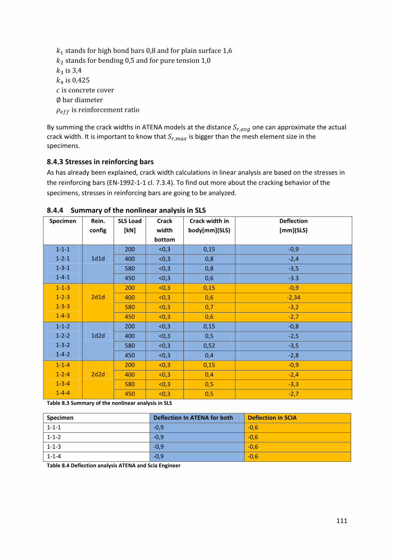
111
𝑘1 stands for high bond bars 0,8 and for plain surface 1,6 𝑘2 stands for bending 0,5 and for pure tension 1,0 𝑘3 is 3,4 𝑘4 is 0,425 𝑐 is concrete cover ∅ bar diameter 𝜌𝑒𝑓𝑓 is reinforcement ratio
By summing the crack widths in ATENA models at the distance 𝑆𝑟,𝑎𝑣𝑔 one can approximate the actual crack width. It is important to know that 𝑆𝑟,𝑚𝑎𝑥 is bigger than the mesh element size in the specimens.
8.4.3 Stresses in reinforcing bars As has already been explained, crack width calculations in linear analysis are based on the stresses in the reinforcing bars (EN-1992-1-1 cl. 7.3.4). To find out more about the cracking behavior of the specimens, stresses in reinforcing bars are going to be analyzed.
8.4.4 Summary of the nonlinear analysis in SLS Specimen Rein.
config SLS Load
[kN] Crack width
bottom
Crack width in body[mm](SLS)
Deflection [mm](SLS)
1-1-1 1-2-1 1-3-1 1-4-1
1d1d
200 <0,3 0,15 -0,9 400 <0,3 0,8 -2,4 580 <0,3 0,8 -3,5 450 <0,3 0,6 -3.3
1-1-3 1-2-3 1-3-3 1-4-3
2d1d
200 <0,3 0,15 -0,9 400 <0,3 0,6 -2,34 580 <0,3 0,7 -3,2 450 <0,3 0,6 -2,7
1-1-2 1-2-2 1-3-2 1-4-2
1d2d
200 <0,3 0,15 -0,8 400 <0,3 0,5 -2,5 580 <0,3 0,52 -3,5 450 <0,3 0,4 -2,8
1-1-4 1-2-4 1-3-4 1-4-4
2d2d
200 <0,3 0,15 -0,9 400 <0,3 0,4 -2,4 580 <0,3 0,5 -3,3 450 <0,3 0,5 -2,7
Table 8.3 Summary of the nonlinear analysis in SLS
Specimen Deflection In ATENA for both Deflection in SCIA 1-1-1 -0,9 -0,6 1-1-2 -0,9 -0,6 1-1-3 -0,9 -0,6 1-1-4 -0,9 -0,6 Table 8.4 Deflection analysis ATENA and Scia Engineer

112
Specimen Deflection In ATENA for both
Deflection in SCIA Deflection in PNL
1-2-1 -2,4 -1,2 -2,8 1-2-2 -2,4 -1,2 -2,8 1-2-3 -2,5 -1,2 -2,8 1-2-4 -2,4 -1,2 -2,8 Table 8.5 Deflection analysis ATENA and Scia Engineer
Specimen Deflection In ATENA for both Deflection in SCIA 1-3-1 -3,5 -1,7 1-3-2 -3,5 -1,7 1-3-3 -3,2 -1,7 1-3-4 -3,2 -1,7 Table 8.6 Deflection analysis ATENA and Scia Engineer
Specimen Deflection In ATENA for both Deflection in SCIA 1-4-1 -3,3 -1,3 1-4-2 -3,0 -1,3 1-4-3 -2,9 -1,3 1-4-4 -3,1 -1,3 Table 8.7 Deflection analysis ATENA and Scia Engineer
RED NOT acceptable according to on Eurocode Green Acceptable according to Eurocode Specimen Load (SLS) Rein.
config Deflection in ATNEA
Deflection in Scia
1-1-1 1-2-1 1-3-1 1-4-1
200 1d1d
-0,9 -0,6 400 -2,44 -1,2 580 -3,5 -1,7 450 -3,3 -1,3
1-1-2 1-2-2 1-3-2 1-4-2
200 1d2d
-0,9 -0,6 400 -2,44 -1,2 580 -3,5 -1,7 450 -3,0 -1,3
1-1-3 1-2-3 1-3-3 1-4-3
200 2d1d
-0,9 -0,6 400 -2,54 -1,2 580 -3,2 -1,7 450 -2,9 -1,3
1-1-4 1-2-4 1-3-4 1-4-4
200 2d2d
-0,9 -0,6 400 -2,44 -1,2 580 -3,2 -1,7 450 -3,1 -1,3
Table 8.8 Deflection analysis ATENA and Scia Engineer
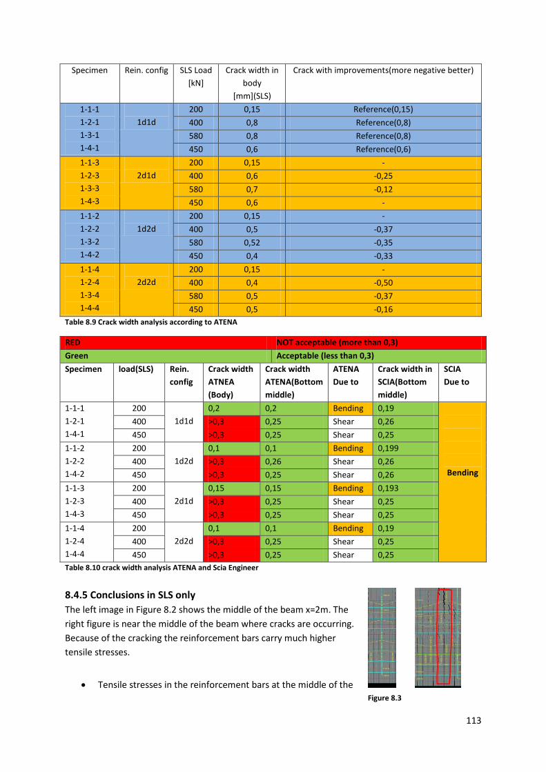
113
Specimen Rein. config SLS Load [kN]
Crack width in body
[mm](SLS)
Crack with improvements(more negative better)
1-1-1 1-2-1 1-3-1 1-4-1
1d1d
200 0,15 Reference(0,15) 400 0,8 Reference(0,8) 580 0,8 Reference(0,8) 450 0,6 Reference(0,6)
1-1-3 1-2-3 1-3-3 1-4-3
2d1d
200 0,15 - 400 0,6 -0,25 580 0,7 -0,12 450 0,6 -
1-1-2 1-2-2 1-3-2 1-4-2
1d2d
200 0,15 - 400 0,5 -0,37 580 0,52 -0,35 450 0,4 -0,33
1-1-4 1-2-4 1-3-4 1-4-4
2d2d
200 0,15 - 400 0,4 -0,50 580 0,5 -0,37 450 0,5 -0,16
Table 8.9 Crack width analysis according to ATENA
RED NOT acceptable (more than 0,3) Green Acceptable (less than 0,3) Specimen load(SLS) Rein.
config Crack width ATNEA (Body)
Crack width ATENA(Bottom middle)
ATENA Due to
Crack width in SCIA(Bottom middle)
SCIA Due to
1-1-1 1-2-1 1-4-1
200 1d1d
0,2 0,2 Bending 0,19
Bending
400 >0,3 0,25 Shear 0,26 450 >0,3 0,25 Shear 0,25
1-1-2 1-2-2 1-4-2
200 1d2d
0,1 0,1 Bending 0,199 400 >0,3 0,26 Shear 0,26 450 >0,3 0,25 Shear 0,26
1-1-3 1-2-3 1-4-3
200 2d1d
0,15 0,15 Bending 0,193 400 >0,3 0,25 Shear 0,25 450 >0,3 0,25 Shear 0,25
1-1-4 1-2-4 1-4-4
200 2d2d
0,1 0,1 Bending 0,19 400 >0,3 0,25 Shear 0,25 450 >0,3 0,25 Shear 0,25
Table 8.10 crack width analysis ATENA and Scia Engineer
8.4.5 Conclusions in SLS only The left image in Figure 8.2 shows the middle of the beam x=2m. The right figure is near the middle of the beam where cracks are occurring. Because of the cracking the reinforcement bars carry much higher tensile stresses.
• Tensile stresses in the reinforcement bars at the middle of the
Figure 8.3

114
beam are lower in ATENA in than in Scia Engineer. The reason for this is that ATENA also considers cracking in the concrete, so it acknowledges that reinforcement bars carry more tensile stresses at places where cracks are occurring (see Annex 8).
• Shear reinforcement has a much bigger impact in controlling the cracks in SLS than the longitudinal reinforcements, including skin reinforcements (tensile and compression). This was anticipated because of the higher number of added shear reinforcements.
• The extra shear reinforcement that is designed with the 2D finite element model in Scia Engineer (reinforcement configuration 1d2d) is necessary for the reinforcement design.
• Skin reinforcements (1d2d and 2d2d) do little in the way of controlling the crack width in the middle of the cross-section of the specimens. This too was also anticipated on the basis of the lower number of extra skin reinforcements.
• The skin reinforcement design with the 2D finite element model in Scia Engineer (reinforcement configuration 2d1d and 2d2d) is not necessary for the reinforcement design.
• The stresses in the reinforcement bars in ATENA vary. ATENA considers cracked concrete, so the stresses in the reinforcement bars are dependent to the place of cracks. Tensile stresses in the reinforcement bars are higher around large cracks.
• In ATENA (SLS) most of the cracks that go beyond the crack width criterion (0.3 mm) are inclined shear cracks. (This is not entirely true because the influence of longitudinal reinforcements and shear reinforcements in controlling cracks of 45 degrees is the same.) That these inclined cracks are being addressed by the shear reinforcements is mostly because of the following practical advantages of shear reinforcements:
1) Additional confinement (EN-1992-1-1 cl.3.1.9(1) ,(2)) 2) Supporting role 3) Smart placing (effective, cost, manpower)
• In Scia, which uses NEN-EN 1992-1-1 art 7.3.3, crack width at the bottom of the cross section
can be calculated on the basis of the tensile stresses in the longitudinal bottom reinforcement bars. This means that a shear reinforcement configuration determined either with or without optimization in the Beam model is not enough to avoid inclined cracks in the middle of the cross section.
• The crack width in the bottom of the cross-section in Scia Engineer and in ATENA both satisfy the crack width criterion in NEN-EN 1992-1-1 Table 7.1N.
• The crack width in the middle of cross-section in SCIA and in ATENA do not satisfy the crack width criterion in NEN-EN 1992-1-1 Table 7.1N, except in case of low level loads (200 kN).
• In specimens that do not satisfy the crack width criterion, the cause of cracking in all of them in SLS is due to shear cracking (Preferably addressed to shear), and is different with Scia Engineer.
• All deflections in specimens at SLS are approximately twice as big as in the Scia Engineer models. This can be explained by the fact that ATENA works with cracked concrete, which has lower stiffness than the un-cracked concrete that Scia Engineer works with (chapter 4.3.3 and annex 4). Lower stiffness of the specimens leads to higher deflection. However, those deflections all easily fall into the range suggested in NEN-EN 1992-1-1 cl. 7.4.
• It should be noted that in Scia Engineer, one usually manually lowers the elasticity module to be able to simulate the real deformation of the structural elements. The comparison of the

115
ATENA results and Scia Engineer results suggests the following allowable elasticity module reduction in Scia Engineer. With these reduction factors in Scia Engineer one can simulate the real deformation of the slender beams. These reduction factors can be used for slender beams with the same reinforcement ratio and cracking area as the specimens that are designed in this thesis. In the next point this result will be compared with NEN 6720 Dutch code [4].
Specimens Applied
load Original E module in Scia [MPa]
E module that gives the real deformation based on ATENA[Mpa]
Allowable reduction factor in Scia
Allowable reduction factor in NEN 6720 art 8.6.3
E Module in PNL [MPa]
1-1-1 1-1-2 1-1-3 1-1-4
200 kN 32800 20000 0,6 0,4-0,6 (instant deformation)
-
1-2-1 1-2-2 1-2-3 1-2-4
400 kN 32800 15000 0,45 0,45-0,53 (instant deformation)
14300
1-4-1 1-4-2 1-4-3 1-4-4
450 kN 32800 13000 0,39 0,33-0,34 (total deformation)
-
Table 8.11 Adjusting E module to get the realistic deformation results in Scia engineering, and comparing with NEN and PNL analysis.
• According to NEN 6720 8.6.1 and 8.6.3 [4] for RC beams with rectangular cross-section that are under bending moment and without axial normal load, the module of elasticity should be reduced by a facto 𝛼. This reduction depends on the reinforcement ratio and can be determined using Table 35 in NEN 6720 cl. 8.6.3. The comparison of the 𝛼 factor with table 8.11 suggests the conclusion that the results from Table 8.11 for low and middle range load level so for 200 kN (with rein. ratios between 0,5% and 0,9%) and 400 kN (with rein. ratios between 1,2% and 1,5%) almost fall in the ‘instant deformation’ (onmiddelijk optredende doorbuiging in Dutch) range or in NEN 6720. For high load levels of 450 kN (with rein. ratios between 1,6% and 1,9%) the results from table 8.11 are in the same range as in NEN 7620 for ‘total deformation’ (totale doorbuiging in Dutch).
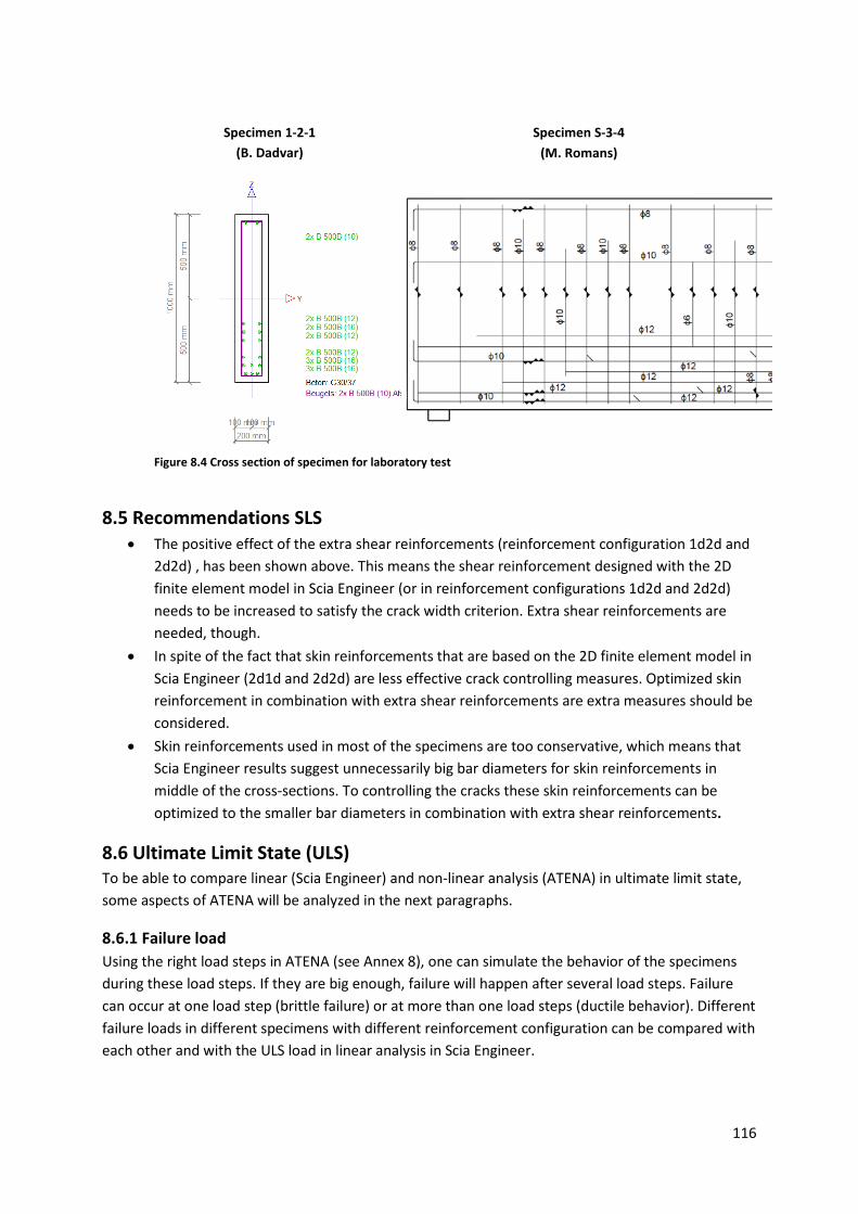
116
Specimen 1-2-1
(B. Dadvar) Specimen S-3-4
(M. Romans)
Figure 8.4 Cross section of specimen for laboratory test
8.5 Recommendations SLS • The positive effect of the extra shear reinforcements (reinforcement configuration 1d2d and
2d2d) , has been shown above. This means the shear reinforcement designed with the 2D finite element model in Scia Engineer (or in reinforcement configurations 1d2d and 2d2d) needs to be increased to satisfy the crack width criterion. Extra shear reinforcements are needed, though.
• In spite of the fact that skin reinforcements that are based on the 2D finite element model in Scia Engineer (2d1d and 2d2d) are less effective crack controlling measures. Optimized skin reinforcement in combination with extra shear reinforcements are extra measures should be considered.
• Skin reinforcements used in most of the specimens are too conservative, which means that Scia Engineer results suggest unnecessarily big bar diameters for skin reinforcements in middle of the cross-sections. To controlling the cracks these skin reinforcements can be optimized to the smaller bar diameters in combination with extra shear reinforcements.
8.6 Ultimate Limit State (ULS) To be able to compare linear (Scia Engineer) and non-linear analysis (ATENA) in ultimate limit state, some aspects of ATENA will be analyzed in the next paragraphs.
8.6.1 Failure load Using the right load steps in ATENA (see Annex 8), one can simulate the behavior of the specimens during these load steps. If they are big enough, failure will happen after several load steps. Failure can occur at one load step (brittle failure) or at more than one load steps (ductile behavior). Different failure loads in different specimens with different reinforcement configuration can be compared with each other and with the ULS load in linear analysis in Scia Engineer.
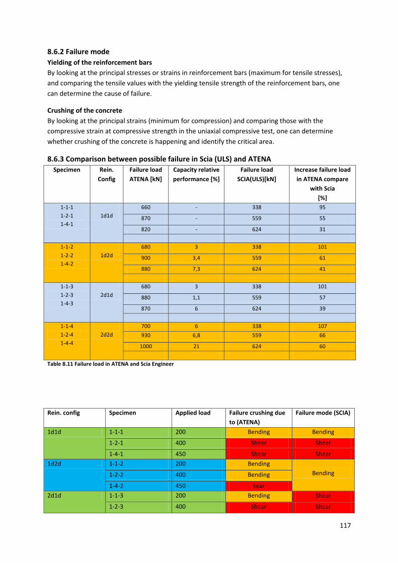
117
8.6.2 Failure mode Yielding of the reinforcement bars By looking at the principal stresses or strains in reinforcement bars (maximum for tensile stresses), and comparing the tensile values with the yielding tensile strength of the reinforcement bars, one can determine the cause of failure.
Crushing of the concrete By looking at the principal strains (minimum for compression) and comparing those with the compressive strain at compressive strength in the uniaxial compressive test, one can determine whether crushing of the concrete is happening and identify the critical area.
8.6.3 Comparison between possible failure in Scia (ULS) and ATENA Specimen Rein.
Config Failure load ATENA [kN]
Capacity relative performance [%]
Failure load SCIA(ULS)[kN]
Increase failure load in ATENA compare
with Scia [%]
1-1-1 1-2-1 1-4-1
1d1d
660 - 338 95
870 - 559 55
820 - 624 31
1-1-2 1-2-2 1-4-2
1d2d
680 3 338 101
900 3,4 559 61
880 7,3 624 41
1-1-3 1-2-3 1-4-3
2d1d
680 3 338 101
880 1,1 559 57
870 6 624 39
1-1-4 1-2-4 1-4-4
2d2d
700 6 338 107 930 6,8 559 66
1000 21 624 60
Table 8.11 Failure load in ATENA and Scia Engineer
Rein. config Specimen Applied load Failure crushing due to (ATENA)
Failure mode (SCIA)
1d1d 1-1-1 200 Bending Bending
1-2-1 400 Shear Shear
1-4-1 450 Shear Shear 1d2d 1-1-2 200 Bending
Bending 1-2-2 400 Bending
1-4-2 450 Sear 2d1d 1-1-3 200 Bending Shear
1-2-3 400 Shear Shear

118
1-4-3 450 Shear Shear 2d2d 1-1-4 200 Bending
Bending 1-2-4 400 Bending
1-4-4 450 Bending
Table 8.12 Failure mode in ATENA and Scia Engineer
8.7 Observations and Conclusions in ULS Only Having chosen the reinforcement configuration 1d1d as a reference point and having compared the rest of the specimens with this one, the following conclusions suggest themselves:
• The Influence of extra shear reinforcements in reinforcement configurations (1d1d to 1d2d
and 2d1d to 2d2d) has more definite positive influence than extra skin reinforcements (1d1d to 2d1d and 1d2d to 2d2d).
• The difference between concrete and reinforcement properties 1 and 2 in ULS is just 6 %, so a ULS failure load with more concrete compressive strength and more yield strength of steel rebars (respectively concrete and reinforcement configuration 2) is 6% higher than concrete and reinforcement properties 1.
• Sometimes extra skin reinforcements in the middle of cross-sections (2d1d and 2d2d) have a positive effect.
• The effect of extra shear reinforcements in specimens (1d1d to 1d2d and 2d1d to 2d2d) does not always mean that there will be extra failure capacity.
• A load level 580 kN is considered ‘out of range’ by GTB 2010 (Chapter 5) because at this load level specimens display ‘brittle failure’. In engineering practice, this is not acceptable.
• The maximum applicable load on the specimen is 450 kN. At this load level the specimens still display ductile behavior.
• At higher load levels, the difference between failure loads in ATENA and in Scia Engineer is smaller.
• All specimens except 1-3-1, 1-3-2, 1-3-3, 1-3-4, 1-1-3, and 1-4-4) show the same behavior in ATENA as in Scia when in the failure mode.
• The ATENA results suggest that for the mid and maximum level loading (400 kN and 450 kN) the governing failure mode, in those specimens with fewer optimized shear bars (1d1d and 2d1d), is crushing of the compression struts due to shear.
• For the highest load level (580 kN) the failure mode suggests the pure crushing of the concrete. None of the reinforcement bars are yielding. At this maximum load, brittle failure may suddenly occur, which can be dangerous. As has been explained in chapter 5, this load is based on GTB 2010 in which the maximum possible reinforcement ratio for C 30/37 is 2,13%. The reinforcement ratio is 2,11% excluding the skin reinforcement (still tensile reinforcement) and 2,38% including skin reinforcement. The ULS results show that in spite of the fact that skin reinforcement has little influence on the cross-section, it should still be counted in the reinforcement ratio.
• As Table 8.11 shows, the resistance to failure which follows from the non-linear analysis is in all specimens higher than the design strength calculated by Scia Engineer.

119
8.8 Conclusions ULS and SLS and Recommendations
8.8.1 Best reinforcement configuration So far the only possible reinforcement configuration based on ATENA results is 1d1d for low level loads (applied load 200 kN SLS). Other configurations do not meet the Eurocode requirement in SLS due to the crack width problem in the middle of the cross-section.
In ATENA the best reinforcement configuration can be determined on the basis of the level of reinforcement (kg/m3) and the maximum load capacity of the specimen before failure.
Specimens Applied
load[kN] Rein.config ATENA SCIA
1-1-1 1-1-2 1-1-3 1-1-4
200 1d1d Meets Eurocode Meets Eurocode 1d2d 2d1d 2d2d
1-2-1 1-2-2 1-2-3 1-2-4
400 1d1d Does not meet Eurocode
Meets Eurocode
1d2d
2d1d
2d2d
1-3-1 1-3-2 1-3-3 1-3-4
580 1d1d Does not meet Eurocode
Meets Eurocode
1d2d
2d1d
2d2d
1-4-1 1-4-2 1-4-3 1-4-4
450 1d1d Does not meet Eurocode
Meets Eurocode
1d2d
2d1d
2d2d Table 8.13
• In ATENA models in SLS, some mesh dependencies can be observed. Mesh dependencies mostly come from the concrete model SBETA that is used in ATENA modeling (see also the recommendation in chapter 6).
• There is a difference 20 to 100% difference between the failure load in SCIA (ULS) and in ATENA. Possible explanations for this gap between failure loads in ATENA and Scia Engineer include: a) Non-linear analysis takes the concrete tensile strength into account b) ATENA takes the favorable effect of confined concrete in the compressive zone in to
account
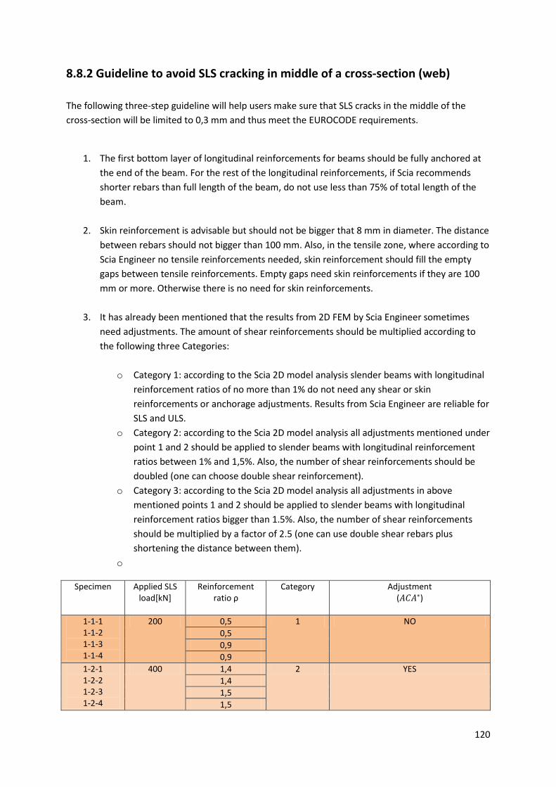
120
8.8.2 Guideline to avoid SLS cracking in middle of a cross-section (web) The following three-step guideline will help users make sure that SLS cracks in the middle of the cross-section will be limited to 0,3 mm and thus meet the EUROCODE requirements.
1. The first bottom layer of longitudinal reinforcements for beams should be fully anchored at the end of the beam. For the rest of the longitudinal reinforcements, if Scia recommends shorter rebars than full length of the beam, do not use less than 75% of total length of the beam.
2. Skin reinforcement is advisable but should not be bigger that 8 mm in diameter. The distance between rebars should not bigger than 100 mm. Also, in the tensile zone, where according to Scia Engineer no tensile reinforcements needed, skin reinforcement should fill the empty gaps between tensile reinforcements. Empty gaps need skin reinforcements if they are 100 mm or more. Otherwise there is no need for skin reinforcements.
3. It has already been mentioned that the results from 2D FEM by Scia Engineer sometimes need adjustments. The amount of shear reinforcements should be multiplied according to the following three Categories:
o Category 1: according to the Scia 2D model analysis slender beams with longitudinal reinforcement ratios of no more than 1% do not need any shear or skin reinforcements or anchorage adjustments. Results from Scia Engineer are reliable for SLS and ULS.
o Category 2: according to the Scia 2D model analysis all adjustments mentioned under point 1 and 2 should be applied to slender beams with longitudinal reinforcement ratios between 1% and 1,5%. Also, the number of shear reinforcements should be doubled (one can choose double shear reinforcement).
o Category 3: according to the Scia 2D model analysis all adjustments in above mentioned points 1 and 2 should be applied to slender beams with longitudinal reinforcement ratios bigger than 1.5%. Also, the number of shear reinforcements should be multiplied by a factor of 2.5 (one can use double shear rebars plus shortening the distance between them).
o
Specimen Applied SLS load[kN]
Reinforcement ratio ρ
Category Adjustment (𝐴𝐶𝐴∗)
1-1-1 1-1-2 1-1-3 1-1-4
200 0,5 1 NO 0,5 0,9 0,9
1-2-1 1-2-2 1-2-3 1-2-4
400 1,4 2 YES 1,4 1,5 1,5

121
1-4-1 1-4-2 1-4-3 1-4-4
450 1,6 3 Yes 1,6 1,9 1,9
Table 8.14 * Avoid Crack Adjustments or ACA
8.8.3 The result from above adjustments in SLS and ULS are as following • After the abovementioned adjustments have been made, there are no differences in SLS and
in moment capacity in Scia Engineer. Only the shear capacity is now a factor approximately 2,0 in category 2 and 2,5 in category 3, higher than without adjustments.
• Table 8.14 shows the failure capacity according to ATENA. With the same concrete and steel properties, ‘Avoiding crack adjustments’ has less than 1% more failure load. This suggests that the abovementioned adjustments to avoid cracking in SLS do not have much impact on failure load in ULS.
8.9 Recommendations • The guideline above should be validated comprehensively by doing a laboratory test on the
basis of new methods of reinforcing as well as the conclusions and recommendations of this thesis.
• Further research is needed to adjust the guideline to slender beams with different dimensions.
• Further research is needed for a full understanding of the influence of bearing size and dimensions on the bearing capacity and behavior of the specimens under applied loads.
• Further research is needed to make more accurate conversions from 2D models in Scia Engineer into 1D modeling.
• Further research is needed for a full understanding of the impact of the free distance between bearings and the edge of the specimens on the bearing capacity and behavior of the specimens under applied loads.
• Further research into PNL analysis of the 1D slender beam is needed. • As this thesis was being written, NEMETSCHEK Scia developed a new program, Scia Design
Forms, for concrete cross sectional analysis. This package contains the following features:
Easy to use for day-to-day design: the user interface is more user-friendly. High-quality calculation reports: detailed calculation reports, especially for interaction with clients engineering practice. Clear output of formulas: mathematical formulas with symbols, substituted numbers and final results are all included in the program Dynamic pictures Interactive workflow: live updates of all results Write your own code checks: the designer can write and share his own checks Integration with Scia Engineer: the input values for a given calculation can be taken directly from Scia Engineer (geometry, loads, etc.)
This program may be very helpful for future researchers in this field.
122
References
[1] “Gewapend Beton” lecture book CT2052, Civil Engineering, TU Delft- Prof.dr.ir.-Ing.h.c. J.C. Walraven, March 2010
[2] ”Design of walls with linear elastic finite element methods” master thesis, TU Delft,
Concrete Structures, Marc Romans April 2010 [3] Report “Finite element Analysis of reinforced concrete structures under Monotonic
Loads” H.G. Kwak and Filip C. Flippou , Civil Engineering, University of California, November 1990
[4] NEN 6720-1995 TGB (Technical fundamentals for building construction) 1990 VBC1995
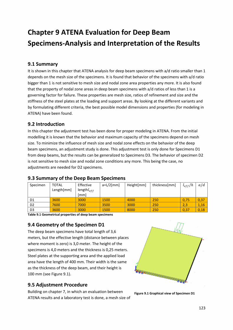
123
Chapter 9 ATENA Evaluation for Deep Beam Specimens-Analysis and Interpretation of the Results
9.1 Summary It is shown in this chapter that ATENA analysis for deep beam specimens with a/d ratio smaller than 1 depends on the mesh size of the specimens. It is found that behavior of the specimens with a/d ratio bigger than 1 is not sensitive to mesh size and nodal zone area properties any more. It is also found that the property of nodal zone areas in deep beam specimens with a/d ratios of less than 1 is a governing factor for failure. These properties are mesh size, ratios of refinement and size and the stiffness of the steel plates at the loading and support areas. By looking at the different variants and by formulating different criteria, the best possible model dimensions and properties (for modeling in ATENA) have been found.
9.2 Introduction In this chapter the adjustment test has been done for proper modeling in ATENA. From the initial modelling it is known that the behavior and maximum capacity of the specimens depend on mesh size. To minimize the influence of mesh size and nodal zone effects on the behavior of the deep beam specimens, an adjustment study is done. This adjustment test is only done for Specimens D1 from deep beams, but the results can be generalized to Specimens D3. The behavior of specimen D2 is not sensitive to mesh size and nodal zone conditions any more. This being the case, no adjustments are needed for D2 specimens.
9.3 Summary of the Deep Beam Specimens Specimen TOTAL
Length[mm] Effective length𝑙𝑒𝑓𝑓 [mm]
a=L/2[mm] Height[mm] thickness[mm] 𝑙𝑒𝑓𝑓/ℎ 𝑎/𝑑
D1 3600 3000 1500 4000 250 0,75 0,37 D2 7600 7000 3500 3000 250 2,3 1,16 D3 3600 3000 1500 8000 250 0,37 0,18
Table 9.1 Geometrical properties of deep beam specimens
9.4 Geometry of the Specimen D1 The deep beam specimens have total length of 3,6 meters, but the effective length (distance between places where moment is zero) is 3,0 meter. The height of the specimens is 4,0 meters and the thickness is 0,25 meters. Steel plates at the supporting area and the applied load area have the length of 400 mm. Their width is the same as the thickness of the deep beam, and their height is 100 mm (see Figure 9.1).
9.5 Adjustment Procedure Building on chapter 7, in which an evaluation between ATENA results and a laboratory test is done, a mesh size of
Figure 9.1 Graphical view of Specimen D1
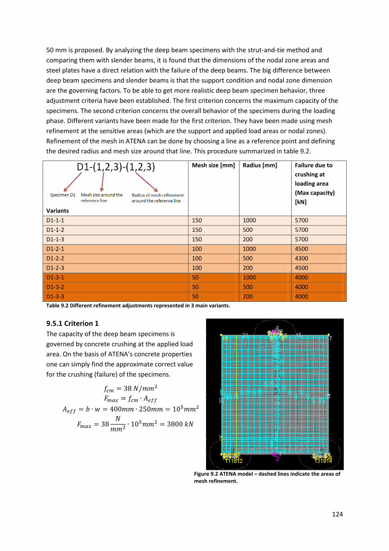
124
50 mm is proposed. By analyzing the deep beam specimens with the strut-and-tie method and comparing them with slender beams, it is found that the dimensions of the nodal zone areas and steel plates have a direct relation with the failure of the deep beams. The big difference between deep beam specimens and slender beams is that the support condition and nodal zone dimension are the governing factors. To be able to get more realistic deep beam specimen behavior, three adjustment criteria have been established. The first criterion concerns the maximum capacity of the specimens. The second criterion concerns the overall behavior of the specimens during the loading phase. Different variants have been made for the first criterion. They have been made using mesh refinement at the sensitive areas (which are the support and applied load areas or nodal zones). Refinement of the mesh in ATENA can be done by choosing a line as a reference point and defining the desired radius and mesh size around that line. This procedure summarized in table 9.2.
Variants
Mesh size [mm] Radius [mm] Failure due to crushing at loading area (Max capacity) [kN]
D1-1-1 150 1000 5700 D1-1-2 150 500 5700 D1-1-3 150 200 5700 D1-2-1 100 1000 4500 D1-2-2 100 500 4300 D1-2-3 100 200 4500 D1-3-1 50 1000 4000 D1-3-2 50 500 4000 D1-3-3 50 200 4000 Table 9.2 Different refinement adjustments represented in 3 main variants.
9.5.1 Criterion 1 The capacity of the deep beam specimens is governed by concrete crushing at the applied load area. On the basis of ATENA’s concrete properties one can simply find the approximate correct value for the crushing (failure) of the specimens.
𝑓𝑐𝑚 = 38 𝑁/𝑚𝑚2 𝐹𝑚𝑎𝑥 = 𝑓𝑐𝑚 ∙ 𝐴𝑒𝑓𝑓
𝐴𝑒𝑓𝑓 = 𝑏 ∙ 𝑤 = 400𝑚𝑚 ∙ 250𝑚𝑚 = 105𝑚𝑚2
𝐹𝑚𝑎𝑥 = 38𝑁
𝑚𝑚2 ∙ 105𝑚𝑚2 = 3800 𝑘𝑁
Figure 9.2 ATENA model – dashed lines indicate the areas of mesh refinement.

125
9.5.2 Criterion 2 The second criterion which can results in the best nonlinear model is the behavior of the specimens during the prescribed deformation or loading phase. This criterion is based on the laboratory tests
that have been done in chapter 7 and on experiments done by Tuchscherer and Asin [2]. The occurrence of bottle-shaped struts is the critical factor for the evaluation of the behavior of the different variants. As Figure 9.3 shows, the behavior of the deep beam specimens with radius of refinement between 200 and 500 mm has the strongest resemblance to the behavior displayed in laboratory tests (figures 9.4 and 9.5). The best behavior is chosen on the basis of the laboratory tests and the logical cracking behavior for specimens with radios of refinements of 200 mm and 500 mm.
Figure 9.4 the cracking behavior of deep beam specimens
Figure 9.5 The cracking behavior of S-2-4 specimen
Figure 9.3 Radius of refinement 200mm (left), 500mm (middle) and 1000 mm (right) at load level 3500 kN

126
9.5.3 Criterion 3 According to the first criterion, also taking into account the effect of confinement of concrete, the maximum capacity of the specimen is about 4000 kN. Table 9.2 demonstrates that variant D1-3-(1,2,3) has the best configuration towards maximum capacity. The reason is that the model can correctly predict the failure load of 4000 kN which is the same as the calculated design failure load for criterion 1. The second criterion shows that the variants D1-3-1 and D1-3-2 give the desirable behavior of the specimens. On the basis of the criteria 1 and 2, variant D1-3-2 has been chosen for further research in this thesis. To allow for a comparison of different reinforcement configurations something extra has to be done. To prevent the crushing of concrete at an early stage before the yielding of the reinforcements and to get more equally distributed stresses at supports and loading areas, the following two options should be considered:
9.5.3.1 Option 1: expand the loading area from 400 mm to 800 mm This adjustment grants the ATENA model more capacity, especially at the loading area. One can simply calculate the impact of this adjustment on the failure capacity load:
𝑓𝑐𝑚 = 38 𝑁/𝑚𝑚2 𝐹𝑚𝑎𝑥 = 𝑓𝑐𝑚 ∙ 𝐴𝑒𝑓𝑓
𝐴𝑒𝑓𝑓 = 𝑏 ∙ 𝑤 = 800𝑚𝑚 ∙ 250𝑚𝑚 = 2 ∙ 105𝑚𝑚2
𝐹𝑚𝑎𝑥 = 38𝑁
𝑚𝑚2 ∙ 2 ∙ 105𝑚𝑚2 = 7600 𝑘𝑁
THIS IS THE SAME THEORETICAL CAPACITY AS IN THE SUPPORTING AREA.
9.5.3.2 Option 2: increase the steel plate height from 100 mm to 200 mm This adjustment makes for a more equal distribution and transfer of stresses due to prescribe deformation at the top middle of the loading plate. For this adjustment three possible variants are considered. Based on the abovementioned options for the adjustment of the boundary conditions at nodal zone areas, in this case steel plates, the following three variants are examined:
Variant 1 This variant uses the original default dimensions that lead to early failure at a load level of 4000 kN. To prevent the crushing of the concrete at an early stage, variants 2 and 3 have been developed.
Figure 9.6 Adjustments for Variant 1 (left), and variant 2(right)
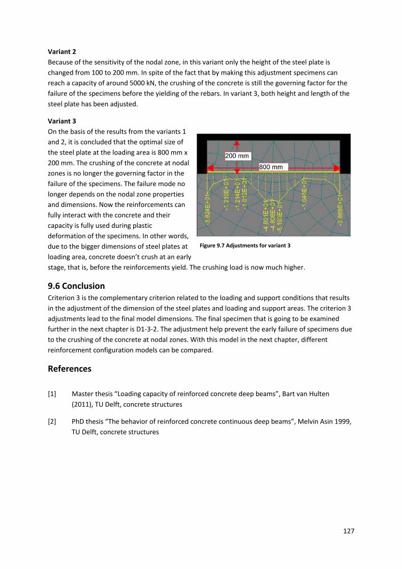
127
Variant 2 Because of the sensitivity of the nodal zone, in this variant only the height of the steel plate is changed from 100 to 200 mm. In spite of the fact that by making this adjustment specimens can reach a capacity of around 5000 kN, the crushing of the concrete is still the governing factor for the failure of the specimens before the yielding of the rebars. In variant 3, both height and length of the steel plate has been adjusted.
Variant 3 On the basis of the results from the variants 1 and 2, it is concluded that the optimal size of the steel plate at the loading area is 800 mm x 200 mm. The crushing of the concrete at nodal zones is no longer the governing factor in the failure of the specimens. The failure mode no longer depends on the nodal zone properties and dimensions. Now the reinforcements can fully interact with the concrete and their capacity is fully used during plastic deformation of the specimens. In other words, due to the bigger dimensions of steel plates at loading area, concrete doesn’t crush at an early stage, that is, before the reinforcements yield. The crushing load is now much higher.
9.6 Conclusion Criterion 3 is the complementary criterion related to the loading and support conditions that results in the adjustment of the dimension of the steel plates and loading and support areas. The criterion 3 adjustments lead to the final model dimensions. The final specimen that is going to be examined further in the next chapter is D1-3-2. The adjustment help prevent the early failure of specimens due to the crushing of the concrete at nodal zones. With this model in the next chapter, different reinforcement configuration models can be compared.
References [1] Master thesis “Loading capacity of reinforced concrete deep beams”, Bart van Hulten (2011), TU Delft, concrete structures
[2] PhD thesis “The behavior of reinforced concrete continuous deep beams”, Melvin Asin 1999, TU Delft, concrete structures
Figure 9.7 Adjustments for variant 3

128
Chapter 10 Comparing SBM, STM, LE-FEM and NL-FEM Reinforcing Methods by Using ATENA for DEEP Beam Specimens
10.1 Summary In this chapter the different reinforcement configurations methods are compared with the ATENA results. Regarding SLS for D1 (a/d<1) deep beam specimens, it is concluded that crack width and deflection are not governing factors. Crack width analysis of D1 specimens shows almost no cracks in SLS. For D2 deep beam specimens (a/d>1) in SLS, crack width’s behavior is more like slender beam specimens. This means that in D2 specimens, crack width in the web is not satisfied. The solution is to double the longitudinal mesh net to cover half of the height of the specimens. For ULS design for D1 specimens, a high failure load is measured in ATENA. The difference between ATENA failure load (ULS ATENA) and ULS design load is sometime the factor 6,7. Explanations for this difference include internal level arm assumption in hand calculations (SBM), different nodal dimensions (STM), the tensile strength of the concrete and the confinement of the concrete. On the other hand, failure load in ATENA for D2 (a/d>1) specimens is just like slender beams, twice as big as the ULS design load. The end of the chapter contains a small investigation into the effective shear height for D1, D2 and D3 specimens. Investigation shows that effective shear height for specimens equals the value ‘d’.
10.2 Introduction The reinforcement of deep beams in practice is usually done on the basis of the SBM method or the LE-FEM. In this chapter will touch on four methods to reinforce the deep beam specimens:
• The Standard Beam Method (SBM) (chapter 2) • The Strut-and-Tie Method (STM) (chapter 2) • The LE-FEM (using Linear elastic module of Scia Engineer-chapter 4 –Annex 1) • The NL-FEM (using None Linear elastic module of Scia Engineer-Chapter 2 –Annex 2)
All four methods are going to be compared with ATENA. This chapter tried to assess which reinforcement method for deep beam specimens is the most efficient. The ATENA results, including visualizations, can be found in Annex 10.
10.3 Table of the Deep Beam Specimens Specimen Total
length [mm] Effective length𝑙𝑒𝑓𝑓 [mm]
a=L/2 [mm]
Height [mm]
Width[mm] 𝑙𝑒𝑓𝑓/ℎ 𝑎/𝑑
D1 3600 3000 1500 4000 250 0,75 0,37 D2 7600 7000 3500 3000 250 2,3 1,16 D3 3600 3000 1500 8000 250 0,37 0,18
Table 10.1

129
10.4 Table of Deep Beam Specimens Based on Reinforcement Configurations
Specimens Reinforcement configurations D1 D1P1SBM
D1P2SBM D1P1STM D1P1STM (Eurocode) D1P2STM D1P2STM (Eurocode) D1P1LFEM D1P2LFEM D1P1NLFEM D1P2NLFEM
D2 D2P1SBM D2P1STM (1) D2P1STM (2) D2P1STM (3) D2P1LFEM D2P1NLFEM
D3 Only conclusions are made based on D1 results Table 10.2
Note: Specimens D1P1STM (Eurocode) and D1P2STM (Eurocode) are designed by taking into account the NEN-EN 1992-1-1 cl.5.6.4 (2), which is explained in chapter 2.6.3.2 of this thesis.
10.5 Serviceability Limit State (SLS) In serviceability limit state the following aspects are going to be investigated:
10.5.1 Deflection Deflection control can easily be carried out from ATENA, and can be compared with Scia Engineer (and/or hand calculation) results. Deflection criteria have been discussed in chapter 8. It was decided to limit the amount of displacement to the value of Span/500.
10.5.2 Crack width Crack width control for deep beam specimens is done according to the following two methods:
1. In SBM and STM the crack width control is done according to NEN EN 1992-1-1 cl 7.2.3, which has been discussed in previous chapters. In these methods crack width is calculated by taking into account the mesh net reinforcements if they are applied at the level where calculation of crack width is taking place.
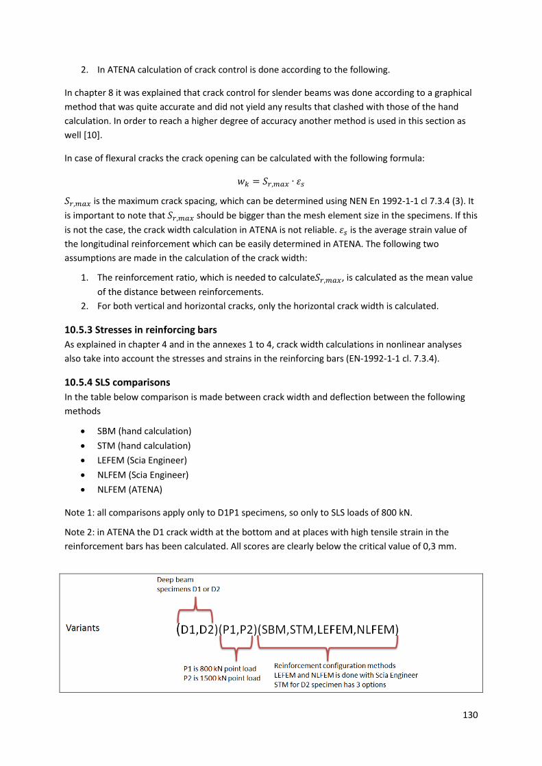
130
2. In ATENA calculation of crack control is done according to the following.
In chapter 8 it was explained that crack control for slender beams was done according to a graphical method that was quite accurate and did not yield any results that clashed with those of the hand calculation. In order to reach a higher degree of accuracy another method is used in this section as well [10].
In case of flexural cracks the crack opening can be calculated with the following formula:
𝑤𝑘 = 𝑆𝑟,𝑚𝑎𝑥 ∙ 𝜀𝑠
𝑆𝑟,𝑚𝑎𝑥 is the maximum crack spacing, which can be determined using NEN En 1992-1-1 cl 7.3.4 (3). It is important to note that 𝑆𝑟,𝑚𝑎𝑥 should be bigger than the mesh element size in the specimens. If this is not the case, the crack width calculation in ATENA is not reliable. 𝜀𝑠 is the average strain value of the longitudinal reinforcement which can be easily determined in ATENA. The following two assumptions are made in the calculation of the crack width:
1. The reinforcement ratio, which is needed to calculate𝑆𝑟,𝑚𝑎𝑥, is calculated as the mean value of the distance between reinforcements.
2. For both vertical and horizontal cracks, only the horizontal crack width is calculated.
10.5.3 Stresses in reinforcing bars As explained in chapter 4 and in the annexes 1 to 4, crack width calculations in nonlinear analyses also take into account the stresses and strains in the reinforcing bars (EN-1992-1-1 cl. 7.3.4).
10.5.4 SLS comparisons In the table below comparison is made between crack width and deflection between the following methods
• SBM (hand calculation) • STM (hand calculation) • LEFEM (Scia Engineer) • NLFEM (Scia Engineer) • NLFEM (ATENA)
Note 1: all comparisons apply only to D1P1 specimens, so only to SLS loads of 800 kN.
Note 2: in ATENA the D1 crack width at the bottom and at places with high tensile strain in the reinforcement bars has been calculated. All scores are clearly below the critical value of 0,3 mm.

131
Variants SLS load [kN]
Displacement [mm]
Crack width at bottom [mm]
ATENA Dis. [mm]
ATENA Crack bottom [mm]
ATENA Crack middle [mm]
Dis criterion [mm]
Crack width criterion [mm]
D1P1SBM 800 - 0,2 0,14 0,012 0,02 6,0 0,3 D1P2SBM 1500 - 0,29 0,27 0,02 0,05 6,0 0,3 D1P1STM 800 - 0,25 0,14 0,012 0,019 6,0 0,3 D1P1STM Eurocode
800 - 0,25 0,14 0,01 small 6,0 0,3
D1P2STM 1500 - 0,28 0,27 0,024 0,04 6,0 0,3 D1P2STM Eurocode
1500 - 0,3 0,27 0,017 small 6,0 0,3
D1P1LEFEM 800 -0,1 - 0,14 0,02 0,04 6,0 0,3 D1P2LEFEM 1500 -0,2 - 0,27 0,019 0,023 6,0 0,3 D1P1NLFEM 800 - - 0,13 0,012 0,027 6,0 0,3 D1P2NLFEM 1500 - - 0,27 0,03 0,06 6,0 0,3 D2P1SBM 800 - 0,26 0,9 0,22 0,4 6,0 0,3 D2P1STM(1) 800 - 0,29 1,2 0,15 0,86 6,0 0,3 D2P1STM(2) 800 - 0,29 1,1 0,15 0,8 6,0 0,3 D2P1STM(3) 800 - 0,24 1,5 0,16 0,6 6,0 0,3 D2P1LEFEM 800 -1,0 - 0,9 0,2 0,4 6,0 0,3 D2P1NLFEM 800 - - 0,9 0,25 0,5 6,0 0,3 Table 10.3 SLS analysis results of ATENA and other reinforcement methods.
Specimens 𝑺𝒓,𝒎𝒂𝒙 ATENA[mm] Bottom
𝑺𝒓,𝒎𝒂𝒙 Hand calculation [mm] bottom
𝜺𝒔𝒕𝒆𝒆𝒍,𝑺𝑳𝑺 ATENA
𝜺𝒔𝒎 − 𝜺𝒄𝒎 NEN-EN 1992.1.1 cl.7.3.4 (2)
D1P1SBM 275 344 4,7 ∙ 10−5 5,8 ∙ 10−4 D1P2SBM 288 340 7,4 ∙ 10−5 8,7 ∙ 10−4 D1P1STM 272 340 4,5 ∙ 10−5 7,35 ∙ 10−4 D1P1STM Eurocode
238 255 4,0 ∙ 10−5 9,8 ∙ 10−4
D1P2STM 322 267 9,1 ∙ 10−5 0,1 ∙ 10−4 D1P2STM Eurocode
236 236 7,2 ∙ 10−5 1,4 ∙ 10−3
Table 10.4 maximum crack spacing and strains of rebars in SLS for ATENA and hand calculation methods (SBM and STM)
10.5.5 Conclusions SLS
• The amount of reinforcement mesh should also be taken into account in calculations of crack width in hand calculation according to NEN EN 1992-1-1 cl 7.2.3 (SBM and STM- if applicable).
• If the dimension of the assumed tensile tie has a little bit difference( about 50 or 60 mm) with the effective height according to NEN-EN 1992-1-1 cl.7.3.2 (3) (which is 2,5(h-d)), it doesn’t matter which of them is used for calculation of effective reinforcement ratio in STM. They both give approximately the same results for crack width.
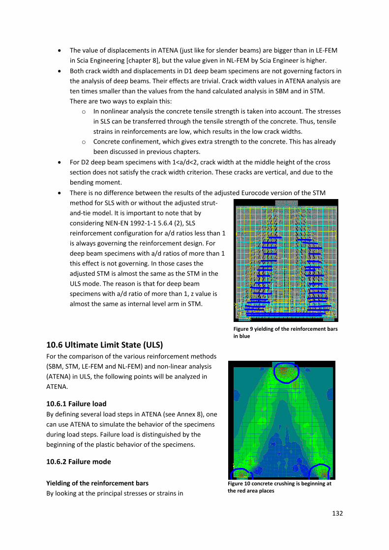
132
• The value of displacements in ATENA (just like for slender beams) are bigger than in LE-FEM in Scia Engineering [chapter 8], but the value given in NL-FEM by Scia Engineer is higher.
• Both crack width and displacements in D1 deep beam specimens are not governing factors in the analysis of deep beams. Their effects are trivial. Crack width values in ATENA analysis are ten times smaller than the values from the hand calculated analysis in SBM and in STM. There are two ways to explain this:
o In nonlinear analysis the concrete tensile strength is taken into account. The stresses in SLS can be transferred through the tensile strength of the concrete. Thus, tensile strains in reinforcements are low, which results in the low crack widths.
o Concrete confinement, which gives extra strength to the concrete. This has already been discussed in previous chapters.
• For D2 deep beam specimens with 1<a/d<2, crack width at the middle height of the cross section does not satisfy the crack width criterion. These cracks are vertical, and due to the bending moment.
• There is no difference between the results of the adjusted Eurocode version of the STM method for SLS with or without the adjusted strut-and-tie model. It is important to note that by considering NEN-EN 1992-1-1 5.6.4 (2), SLS reinforcement configuration for a/d ratios less than 1 is always governing the reinforcement design. For deep beam specimens with a/d ratios of more than 1 this effect is not governing. In those cases the adjusted STM is almost the same as the STM in the ULS mode. The reason is that for deep beam specimens with a/d ratio of more than 1, z value is almost the same as internal level arm in STM.
10.6 Ultimate Limit State (ULS) For the comparison of the various reinforcement methods (SBM, STM, LE-FEM and NL-FEM) and non-linear analysis (ATENA) in ULS, the following points will be analyzed in ATENA.
10.6.1 Failure load By defining several load steps in ATENA (see Annex 8), one can use ATENA to simulate the behavior of the specimens during load steps. Failure load is distinguished by the beginning of the plastic behavior of the specimens.
10.6.2 Failure mode Yielding of the reinforcement bars By looking at the principal stresses or strains in
Figure 9 yielding of the reinforcement bars in blue
Figure 10 concrete crushing is beginning at the red area places
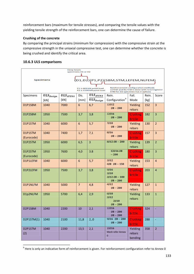
133
reinforcement bars (maximum for tensile stresses), and comparing the tensile values with the yielding tensile strength of the reinforcement bars, one can determine the cause of failure.
Crushing of the concrete By comparing the principal strains (minimum for compression) with the compressive strain at the compressive strength in the uniaxial compressive test, one can determine whether the concrete is being crushed and identify the critical area.
10.6.3 ULS comparisons
Specimens 𝑼𝑳𝑺𝑫𝒆𝒔𝒊𝒈𝒏 [kN]
𝑼𝑳𝑺𝑨𝑻𝑬𝑵𝑨 [kN]
Dis. [mm]
𝑼𝑳𝑺𝑨𝑻𝑬𝑵𝑨𝑼𝑳𝑺𝑫𝒆𝒔𝒊𝒈𝒏
Rein. Configuration9
Fail. Mode
Rein. [kg]
Score
D1P1SBM 1040 7000 6 6,7 12∅𝟏𝟐 ∅𝟖 − 𝟐𝟎𝟎
Yielding rebars
152 3
D1P2SBM 1950 7500 3,7 3,8 12∅𝟏𝟔 ∅𝟖 − 𝟐𝟎𝟎
Crushing brittle
182 3
D1P1STM 1040 6000 6 5,7 7∅𝟏𝟎 ∅𝟖 − 𝟐𝟎𝟎
Yielding rebars
130 2
D1P1STM (Eurocode)
1040 7400 1,7 7,1 8∅𝟏𝟔 ∅𝟖 − 𝟐𝟎𝟎
Crushing brittle
157 3
D1P2STM 1950 6000 6,5 3 8∅𝟏𝟐 ∅𝟖 − 𝟐𝟎𝟎 Yielding rebars
139 2
D1P2STM (Eurocode)
1950 7600 4,0 3.8 𝟏𝟐∅𝟏𝟔 ∅𝟖− 𝟐𝟎𝟎
Crushing brittle
180 3
D1P1LEFM 1040 6000 6 5,7 2∅𝟏𝟐 4∅𝟖 ∅𝟖 − 𝟏𝟓𝟎
Yielding rebars
153 4
D1P2LEFM 1950 7500 3,7 3,8 5∅𝟏𝟔 2∅𝟏𝟎 2∅𝟏𝟐 ∅𝟖 − 𝟏𝟎𝟎
∅𝟖 − 𝟐𝟎𝟎
Crushing brittle
203 4
D1P1NLFM 1040 5000 7 4,8 4∅𝟏𝟐 ∅𝟖 − 𝟐𝟎𝟎
Yielding rebars
127 1
D1p2NLFM 1950 5700 6,4 2,9 6∅𝟏𝟎 2∅𝟏𝟐
𝟐∅𝟏𝟎 ∅𝟖 − 𝟐𝟎𝟎
Yielding rebars
133 1
D2P1SBM 1040 2200 10 2,1 12∅𝟏𝟔 ∅𝟖 − 𝟐𝟎𝟎 ∅𝟖 − 𝟐𝟎𝟎
Crushing brittle
324 -
D2P1STM(1) 1040 2100 11,8 2,.0 9∅𝟏𝟔 ∅𝟖 − 𝟐𝟎𝟎 ∅𝟖 − 𝟐𝟎𝟎
Crushing brittle
288 -
D2P1STM (2)
1040 2200 13,5 2,1 10∅𝟏𝟔 Mesh refer Annex 0
Yielding rebars bending
358 2
9 Here is only an indicative form of reinforcement is given. For reinforcement configuration refer to Annex 0

134
D2P1STM (3)
1040 2200 14 2,1 10∅𝟏𝟔 Mesh refer annex 0
Yielding rebars bending
367 3
D2P1LEFEM 1040 2200 12 2,1 5∅𝟏𝟔 4∅𝟏𝟐 2∅𝟖 ∅𝟖 − 𝟏𝟎𝟎
∅𝟖 − 𝟐𝟎𝟎
Crushing brittle
310 -
D2P1NLFEM 1040 1950 13 1,9 4∅𝟏𝟎 4∅𝟏𝟐 4∅𝟏𝟔1 ∅𝟖 − 𝟐𝟎𝟎
∅𝟖 − 𝟐𝟎𝟎
Yielding rebars bending
270 1
Table 10.5 ULS analysis of ATENA and other design methods
10.6.4 Conclusions related to ULS related to D1 (a/d<1) deep beam specimens
• The failure mode as a result of the yielding of the bars in D1 deep beam specimens in ATENA is the governing failure mode. This is mainly due to the effect of shear stresses. A shear resistance design is included into the calculation of STM within the design of compression struts. In SBM shear resistance design is based on Eurocode. Shear stresses in combination with compression struts (direct transfer of forces from applied load area to the support area) can be visualized as bottle shape effects of tensor trajectories in the specimens.
• All methods to reinforce D1 deep beam specimens generally lead to extra capacity (factor between 4,8 and 6,7). This suggests that all methods are conservative.
• The first explanation for this huge difference between ULS design in hand calculations and ATENA analysis concerns the internal level arm. The internal level arm in the SBM method is based on NABY NEN-EN 1992-1-1 cl6.1 (10) or NEN 6720 cl 8.1.4. ,𝑧 = 0,2𝑙 + 0,4ℎ ≤ 0,6𝑙 , 𝑧 ≤ 0,8𝑙 . With ATENA results it can be shown that the internal level arm is much bigger than is assumed in the SBM method. A simple calculation including the effect of web reinforcements shows that this difference between the internal level arm has factor 3,7 influence in the ULS load in ATENA analysis. Figure 17.2 shows the differences between ATENA analysis and SBM method or hand calculation analysis.
𝐼𝑛 𝑆𝐵𝑀 𝑚𝑒𝑡ℎ𝑜𝑑 𝑀𝐸𝑑(𝑆𝐵𝑀) = 𝑧1𝐹1
𝐼𝑛 𝐴𝑇𝐸𝑁𝐴 𝑎𝑛𝑎𝑙𝑠𝑦𝑠𝑖𝑠 𝑀𝐸𝑑(𝐴𝑇𝐸𝑁𝐴) = 𝑧2𝐹1 + 𝑧3𝐹2
Figure 10.4 bottle shape stress-strain tensor and shear stresses at 3 different cuts
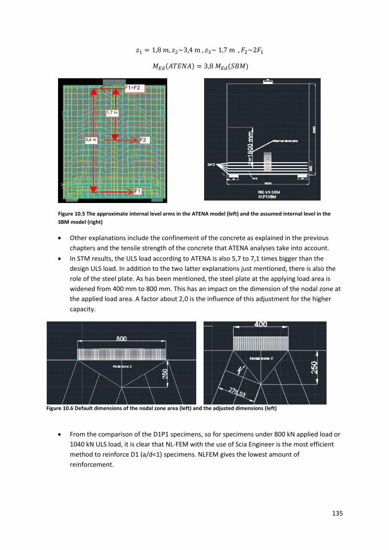
135
𝑧1 = 1,8 𝑚, 𝑧2~3,4 m , 𝑧3~ 1,7 m ,𝐹2~2𝐹1
𝑀𝐸𝑑(𝐴𝑇𝐸𝑁𝐴) = 3,8 𝑀𝐸𝑑(𝑆𝐵𝑀)
Figure 10.5 The approximate internal level arms in the ATENA model (left) and the assumed internal level in the SBM model (right)
• Other explanations include the confinement of the concrete as explained in the previous chapters and the tensile strength of the concrete that ATENA analyses take into account.
• In STM results, the ULS load according to ATENA is also 5,7 to 7,1 times bigger than the design ULS load. In addition to the two latter explanations just mentioned, there is also the role of the steel plate. As has been mentioned, the steel plate at the applying load area is widened from 400 mm to 800 mm. This has an impact on the dimension of the nodal zone at the applied load area. A factor about 2,0 is the influence of this adjustment for the higher capacity.
Figure 10.6 Default dimensions of the nodal zone area (left) and the adjusted dimensions (left)
• From the comparison of the D1P1 specimens, so for specimens under 800 kN applied load or 1040 kN ULS load, it is clear that NL-FEM with the use of Scia Engineer is the most efficient method to reinforce D1 (a/d<1) specimens. NLFEM gives the lowest amount of reinforcement.

136
• The most reliable methods to reinforce D1 deep beams are NL-FEM and STM, because even at high design loads D1P2 (1500 kN applied load or 1950 kN ULS) these two methods lead to the plastic deformation before failure.
• About the Eurocode version of STM, which is based on NEN-EN 1992-1-1 5.6.4 (2), we can conclude that SLS design for deep beam specimens with a/d ratios of less than 1 is always governing reinforcement design. This is the case because in specimens with a/d<1 the angle difference between the compression strut and ties is big (figure 10.7). This leads to higher forces in ties, and requires a higher number of longitudinal reinforcements (theoretically the same number as in SBM). The results from table 10.5 shows that one can use fewer tie reinforcements when NEN-EN 1992-1-1 cl.5.6.4 (2) is ignored. This means that the specimen has enough ultimate capacity and that the crack width criterion still satisfies the Eurocode requirements if one uses the default ULS strut and tie model in SLS design of STM. This suggests the following conclusion: in STM (a/d<1), it is not necessary to use another adjusted strut-and-tie model based on NEN-EN 1992-1-1 5.6.4 (2) (in SLS).
Figure 10.7 Strut-and-tie model for SLS (left) and ULS (right)
• About the specimens with a/d ratios of more than 1, so for D2 specimen, the Eurocode
version and the default version of STM both lead to the same results because the angles between the compression strut and ties are approximately the same. This means that when the a/d ratio is bigger than 1, one can simply ignore the NEN-EN 1992-1-1 5.6.4 (2). There is no need to construct another STM for SLS design (see figure 10.8).

137
Figure 10.8 Strut-and-tie models for ULS (top) SLS (bottom)
• The governing factors for all D1 (a/d<1) deep beam specimens are the dimensions and situations at support and applied load areas. The dimensions of the supports and applied load areas are directly related to the failure load. In spite of plastic deformation, failure always happens at the support or at the applied load area (sensitive nodal zones).
• For D1 (a/d<1) deep beam specimens the effect of support and load area conditions are local. This conclusion is especially important for higher walls. The local disturbance of stresses due to the structure’s high nonlinear behavior in the discontinuity regions is characteristic of deep beam specimens. This effect for high walls will be briefly addressed in the next section.
• Table 10.5 makes clear that for high design load for D1 deep beam specimens almost the same amount of reinforcements is being used, regardless of the design load. This confirms the previous conclusion that support, applied load conditions and dimensions are always the governing factors. This is why almost the same number of reinforcements for higher loads is being used.
• SBM and LE-FEM are the least efficient with regard to the number of reinforcements for D1 deep beam specimens. The amount of reinforcement in NL-FEM is about 25 kg less than the amount of reinforcement that is used on the basis of SBM. This difference is not big for deep beams, which have only one span. Continuous deep beams will sometimes be used in real structures. In those cases this difference in the amount of reinforcement is probably higher. This can be an important governing factor in the choice between different reinforcement configuration methods.
10.6.5 Conclusions related to ULS related to D2 (1<a/d<2) deep beam specimens • ULS ATENA loads for D2 Specimens are all twice as big as the ULS design load. This result is
the same as the results from slender beam specimens in chapter 8. Possible explanations include the following: a) Non-linear analysis takes the concrete tensile strength into account

138
b) ATENA takes the favorable effect of confined concrete in the compressive zone into account
• The best reinforcement configuration is based on NL-FEM with the help of Scia Engineer and option 2 and option 3 from the STM methods. The amount of reinforcement that is used on the basis of NL-FEM is about 50 kg less than in SBM. This difference for one span deep beam is not a major governing factor. However, in continuous deep beams this can be an important governing factor for the choice between different analysis methods.
• Reinforcement configurations SBM and LE-FEM are both acceptable because they have resulted in a capacity which is twice as big as the ULS design load, but they are not efficient. Efficiency is about the number of reinforcements and the plastic behavior of the specimens that indicates that the capacity of the reinforcements is also used in the design of the specimens.
10.7 Shear Effective Height The shear resistance of the deep beams is calculated only in SBM (hand calculation) according to NEN-EN 1992-1-1 cl.6.2.2 (1) and cl. 6.2.3(3). In all other hand calculation methods, like STM, the determination of the shear resistance of the specimens is already included in the calculation procedures. Because of the nonlinear behavior of the deep beam specimens, one can ask whether the shear effective height is the same in linear analysis (normal slender beams). This is investigated in this chapter with the help of nonlinear analysis software package (ATENA).
10.7.1 Arguments Two kinds of shear effective height have been examined: shear effective height in ULS design and shear effective height in ULS ATENA. According to the background document for EC-2[3], the formulations in Eurocode to determine shear capacity and shear reinforcements are based on slender beam specimens. For deep beam specimens other methods of analysis, like the strut-and-tie method are recommended. This may raise the question whether using Eurocode in the SBM method and discussing the actual shear effective height for deep beam specimens is the right line of argument.
10.7.2 Procedure The effective shear height of various deep beam specimens is examined with a nonlinear software package. Table 10.6 shows the results based on ULS design load and on ULS ATENA. It can be seen from the Figures 10.9, 10.10 and 10.11 that the shear effective height for D1, D2 and D3 specimens is more or less equal to the effective height ‘d’ of the cross section. This can be partly explained by the discontinuity regions at the bottom and top of the deep beam specimens. This value is taken into account in SBM’s calculation of shear reinforcements according to NEN-EN 1992-1-1 cl6.2.2 formula 6.2.a,b.
Figure 10.7 shear stresses near by support area

139
In SBM the following formula suffices to find the effective height of the short wall specimen.
𝑧 = 0,2𝑙 + 0,4ℎ ≤ 0,6𝑙 (𝑐ℎ𝑎𝑝𝑡𝑒𝑟 2) 𝑧 ≤ 0,6 𝑙 (𝑐ℎ𝑎𝑝𝑡𝑒𝑟 2) 𝑧 ≤ 0,8 ℎ (𝑐ℎ𝑎𝑝𝑡𝑒𝑟 2)
𝑑 = ℎ − 𝑧2
According to paragraph 6.2 a,b of the Eurocode, shear reinforcements is necessary for D1 specimens under high loads (1500 kN). According to the ATENA analysis, the effective shear height is ‘d’. When using the ‘d’ value in the formulas 6.8 and 6.9 from NEN-EN 1992-1-1, the following results are important:
• The 𝜃 value for using formulas in 6.8 and 6.9 is based on Figure 10.8 is set to be 67 degrees.
• Formula 6.8 from NEN-EN 1992-1-1 can be rewritten as follows:
𝐴𝑠,𝑛𝑒𝑒𝑑𝑒𝑑 = 𝑉𝑅𝑑,𝑠∙𝑠𝑧∙𝑓𝑦𝑤𝑑∙𝑐𝑜𝑡𝜃
In this formula, 𝑉𝑅𝑑,𝑠 = 𝛽𝑉𝐸𝑑
- 𝛽 can be found on the basis of NEN-EN 1991-1-1 cl.6.2.2 (6) - Value 𝑠 is the assumed distance of the shear reinforcement - 𝑓𝑦𝑤𝑑 is the yield strength of the steel, which is 435 𝑁/𝑚𝑚2 - 𝑧 for z value, based on the ATENA results figure 10.9 for both cases of ULS design and ULS ATENA, the value “d” is used
• Formula NEN-EN 1992-1-1 (6.9)
𝑉𝑅𝑑,𝑚𝑎𝑥 = 𝛼𝑐𝑤𝑏𝑤𝑧𝑣1𝑓𝑐𝑑/(𝑐𝑜𝑡𝜃 + 𝑡𝑎𝑛𝜃)
The values of 𝜃 and 𝑧 the same as in the formula in 6.8. This results to the fact that 𝑉𝑅𝑑,𝑚𝑎𝑥 is never a governing factor because of the high value in comparison with 𝑉𝑅𝑑,𝑠.
• In ATENA failure load the effective shear height for D3 specimens is ‘d’. LE-FEM too, (see figure 10.10) shows that effective shear height is ‘d’. The formula from NEN-EN 1992-1-1 (6.2 a, b) to calculate the shear resistance leads to the conclusion that there is no need for extra shear reinforcements in D3 specimens. It is very important to mention that an effective shear height of ‘d’ gives the reasonable results in ULS analysis which has already been discussed.
Figure10.9 D1 specimen in ULS design (left) and in Failure ATENA (right)
Figure 10.8 Tie arch model in SBM and approximation of the 𝜽 value in the deep beam specimens D1 and D3
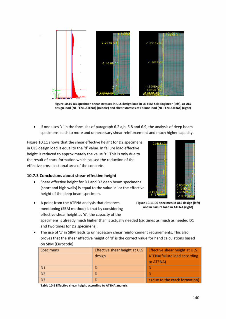
140
.
• If one uses ‘z’ in the formulas of paragraph 6.2 a,b, 6.8 and 6.9, the analysis of deep beam
specimens leads to more and unnecessary shear reinforcement and much higher capacity.
Figure 10.11 shows that the shear effective height for D2 specimens in ULS design load is equal to the ‘d’ value. In failure load effective height is reduced to approximately the value ‘z’. This is only due to the result of crack formation which caused the reduction of the effective cross-sectional area of the concrete.
10.7.3 Conclusions about shear effective height • Shear effective height for D1 and D2 deep beam specimens
(short and high walls) is equal to the value ‘d’ or the effective height of the deep beam specimen.
• A point from the ATENA analysis that deserves mentioning (SBM method) is that by considering effective shear height as ‘d’, the capacity of the specimens is already much higher than is actually needed (six times as much as needed D1 and two times for D2 specimens).
• The use of ‘z’ in SBM leads to unnecessary shear reinforcement requirements. This also proves that the shear effective height of ‘d’ is the correct value for hand calculations based on SBM (Eurocode). Specimens Effective shear height at ULS
design Effective shear height at ULS ATENA(failure load according to ATENA)
D1 D D D2 D D D3 D z (due to the crack formation) Table 10.6 Effective shear height according to ATENA analysis
Figure 10.10 D3 Specimen shear stresses in ULS design load in LE-FEM Scia Engineer (left), at ULS design load (NL-FEM, ATENA) (middle) and shear stresses at Failure load (NL-FEM ATENA) (right)
Figure 10.11 D2 specimen in ULS design (left) and in Failure load in ATENA (right)
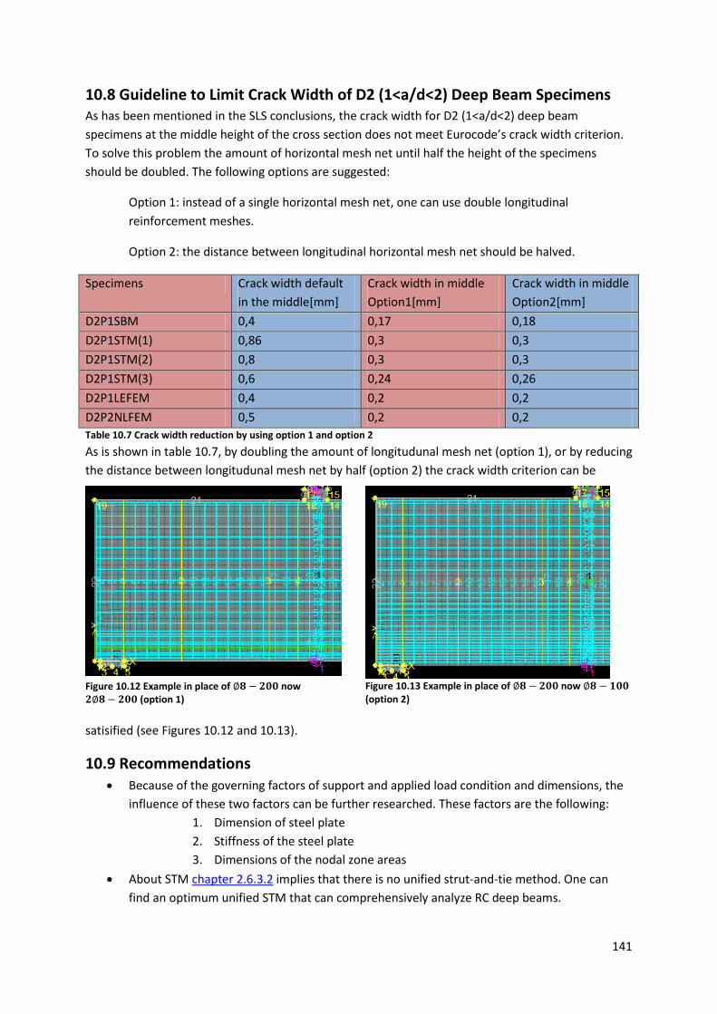
141
10.8 Guideline to Limit Crack Width of D2 (1<a/d<2) Deep Beam Specimens As has been mentioned in the SLS conclusions, the crack width for D2 (1<a/d<2) deep beam specimens at the middle height of the cross section does not meet Eurocode’s crack width criterion. To solve this problem the amount of horizontal mesh net until half the height of the specimens should be doubled. The following options are suggested:
Option 1: instead of a single horizontal mesh net, one can use double longitudinal reinforcement meshes.
Option 2: the distance between longitudinal horizontal mesh net should be halved.
Table 10.7 Crack width reduction by using option 1 and option 2
As is shown in table 10.7, by doubling the amount of longitudunal mesh net (option 1), or by reducing the distance between longitudunal mesh net by half (option 2) the crack width criterion can be
satisified (see Figures 10.12 and 10.13).
10.9 Recommendations • Because of the governing factors of support and applied load condition and dimensions, the
influence of these two factors can be further researched. These factors are the following: 1. Dimension of steel plate 2. Stiffness of the steel plate 3. Dimensions of the nodal zone areas
• About STM chapter 2.6.3.2 implies that there is no unified strut-and-tie method. One can find an optimum unified STM that can comprehensively analyze RC deep beams.
Specimens Crack width default in the middle[mm]
Crack width in middle Option1[mm]
Crack width in middle Option2[mm]
D2P1SBM 0,4 0,17 0,18 D2P1STM(1) 0,86 0,3 0,3 D2P1STM(2) 0,8 0,3 0,3 D2P1STM(3) 0,6 0,24 0,26 D2P1LEFEM 0,4 0,2 0,2 D2P2NLFEM 0,5 0,2 0,2
Figure 10.12 Example in place of ∅𝟖 − 𝟐𝟎𝟎 now 𝟐∅𝟖 − 𝟐𝟎𝟎 (option 1)
Figure 10.13 Example in place of ∅𝟖 − 𝟐𝟎𝟎 now ∅𝟖 − 𝟏𝟎𝟎 (option 2)
142
• There is a program called “CAST” (Computer Aided Strut-and-Tie).This program has a graphical design tool and makes the design process in STM more efficient. The ACI 318-08 design procedure is incorporated in this program. One can assess the efficiency and use of this program within the Eurocode and other STM design procedures.
References
[1] “Gewapend Beton” lecture book CT2052 Prof.dr.ir.-ing.h.c. J.C. Walraven, TU Delft, March 2010
[2] Eurocode 2: Design of concrete structures Part 1-1: General rules and rules for buildings NEN-EN-1992-1-1
[3] Background document for EC-2, Chapter 6.2 Shear, J.C. Walraven, TU Delft, January 2012

143
Chapter 11 Conclusions and recommendations
11.1 introduction This chapter gives conclusions and recommendations related to the objectives and scope of this thesis, which are as follows:
• To improve the reinforcement design method in the LE-FEM, for slender and deep beams. • To investigate whether the results from LE-FEM represent the actual behavior. • To investigate the possible use of nonlinear finite element analysis with Scia Engineer. • To investigate and compare different design methods for analyzing deep beam specimens.
Figure 11.1 Tree chart for designing slender and deep beams with the help of a LE-FEM software package
11.2 Conclusions for Slender beams • Romans claimed that by using the normal reinforcement method in LE-FEM for high slender
beam specimens (in this thesis a high slender beam has height of at least 1,0 meter), the crack width criterion at the bottom of the cross-section might not be met. In this thesis a new reinforcement design method in LE-FEM is introduced. The Main feature of this method is that one gradually adds (step by step) reinforcement at the bottom part of a slender beam. It is demonstrated that the crack width criterion at the bottom can now be met without
Slender beams L/h≥3
Using 'step by step' design in LE-FEM
specimens with high height h~1 m
cracks in the web
Use guideline
Deep beams L/h<3
Deep beams a/d<1
Using 'step by step' design in LE-FEM &NL-
FEM
ULS and SLS control OK
Deep beams a/d>1
Using 'step by step' design in LE-FEM &NL-
FEM
cracks in the web
Double amount of skin rein. till half
height of the specimens

144
laborious iteration procedure.
• Nonlinear analysis of slender beams using the step by step method in LE-FEM shows that the crack width in the web might not satisfy the crack width criterion. To resolve this problem a guideline is introduced (figure 11.2). The main recommendations are as follows:
1. Upper limit for bar diameter of skin reinforcement (8 mm) 2. Upper limit for distance between skin reinforcement in the web (100 mm) 3. Lower limit for the length of the rebars (0,75 ∙ 𝑡𝑜𝑡𝑎𝑙 𝑠𝑝𝑎𝑛) 4. Multiplying the amount of shear reinforcement by a specific factor depending on the
reinforcement ratio (table 11.1)
Figure 11.2 occurring of the cracks in the web of the slender beam specimens
Reinforcement ratio ρ Multiplication factor ρ <1,0 1,0 1<ρ<1,5 2,0 ρ >1,5 2,5 Table 11.1 multiplication factor for amount of shear reinforcement
• In nonlinear analysis a higher ULS capacity in comparison with a hand calculation result is found. The main reason is that after cracking, part of the tensile force is carried by cracked concrete state that is in the softening branch (figure 11.3).
Figure 11.3 Uniaxial stress, strain law
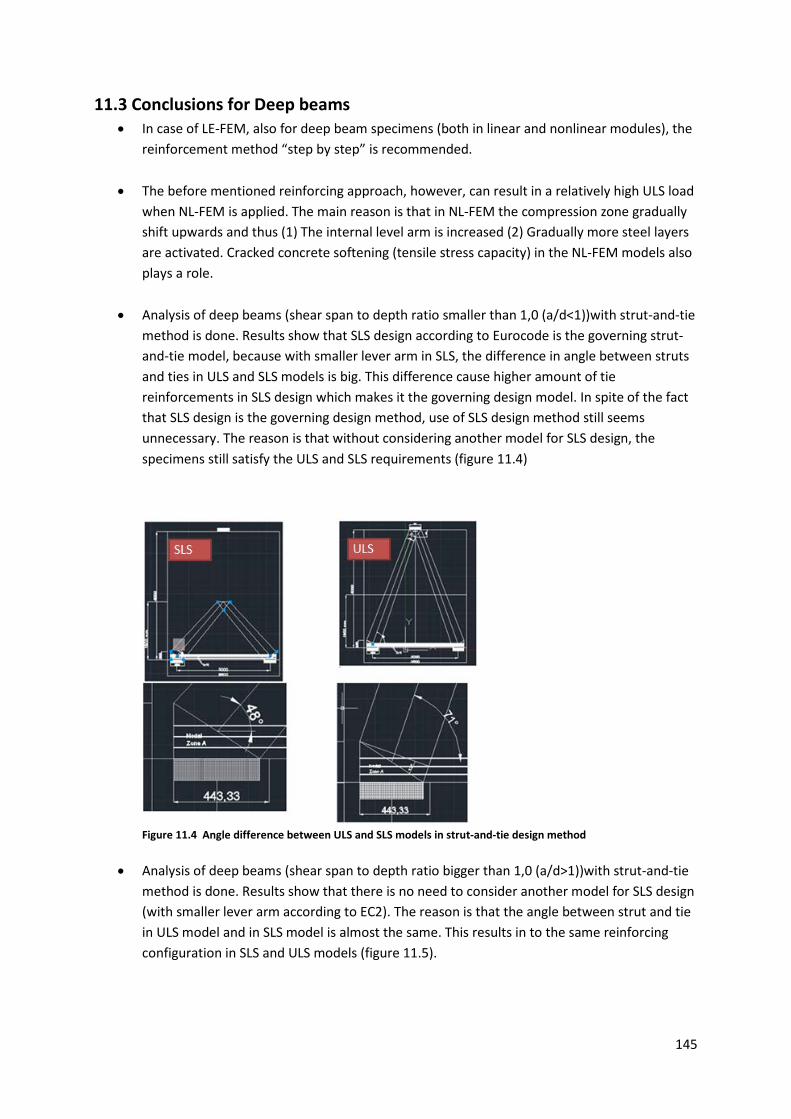
145
11.3 Conclusions for Deep beams • In case of LE-FEM, also for deep beam specimens (both in linear and nonlinear modules), the
reinforcement method “step by step” is recommended.
• The before mentioned reinforcing approach, however, can result in a relatively high ULS load when NL-FEM is applied. The main reason is that in NL-FEM the compression zone gradually shift upwards and thus (1) The internal level arm is increased (2) Gradually more steel layers are activated. Cracked concrete softening (tensile stress capacity) in the NL-FEM models also plays a role.
• Analysis of deep beams (shear span to depth ratio smaller than 1,0 (a/d<1))with strut-and-tie method is done. Results show that SLS design according to Eurocode is the governing strut-and-tie model, because with smaller lever arm in SLS, the difference in angle between struts and ties in ULS and SLS models is big. This difference cause higher amount of tie reinforcements in SLS design which makes it the governing design model. In spite of the fact that SLS design is the governing design method, use of SLS design method still seems unnecessary. The reason is that without considering another model for SLS design, the specimens still satisfy the ULS and SLS requirements (figure 11.4)
Figure 11.4 Angle difference between ULS and SLS models in strut-and-tie design method
• Analysis of deep beams (shear span to depth ratio bigger than 1,0 (a/d>1))with strut-and-tie method is done. Results show that there is no need to consider another model for SLS design (with smaller lever arm according to EC2). The reason is that the angle between strut and tie in ULS model and in SLS model is almost the same. This results in to the same reinforcing configuration in SLS and ULS models (figure 11.5).

146
Figure 11.5 Angle difference between ULS and SLS models in strut-and-tie design method
• This leads to the conclusion that in strut-and-tie analysis for deep beam specimens, it is not
necessary to make different models for SLS and ULS. This is in contrary to Eurocode 2 which suggests that one have to use another strut and tie model for SLS design based on linear elastic theory.
• NL-FEM analysis for deep beam specimens (SLS) with a shear span to depth ratio smaller than 1,0 (a/d<1) , shows that the crack width might be much smaller than in a hand calculation. As mentioned before, see figure 11.3, using tension softening and smeared cracks implies that cracked concrete might still transfer a relatively high tensile stress, even at high strains. As a result, tensile stresses in the reinforcement crossing the cracks are low and the crack width is relatively small.
• NL-FEM analysis for deep beam specimens (SLS) with a shear span to depth ratio bigger than 1,0 (a/d>1), shows that the crack width at the web of the cross section does not satisfy the crack width criterion. To resolve this problem a guideline is introduced. This guideline is basically based on doubling the amount of longitudinal mesh net (relative to default mesh reinforcement from EC2) till the half of the height of specimens.
11.4 Recommendations • To be able to get the best practical reinforcement design in LE-FEM and NL-FEM for both
slender and deep beam specimens, it is recommended to use the step by step reinforcing method.
• In deep beam specimens with an a/d ratio smaller than 1, the properties of the loaded nodal zone areas and boundary conditions have a governing effect on the behavior of the specimens in ULS and SLS (local crushing of the concrete). Further research in this area is recommended.

147
• New laboratory test both for slender and deep beams is recommended. These laboratory tests could verify the step-by-step reinforcement design method introduced in this thesis.
• Using a nonlinear module (pressure only 2D members) in a LE-FEM, for reinforcement design is a promising replacement for laborious nonlinear analysis. Further research on the use of nonlinear modules in Scia Engineer is recommended.