Embed Size (px)
Citation preview

Development of a Six Sigma Transceiver Design Tool
By
James M. Hart
A MASTER OF ENGINEERING REPORT
Submitted to the College of Engineering at
Texas Tech University in
Partial Fulfillment of
The Requirements for the
Degree of
MASTER OF ENGINEERING
Approved
______________________________________ Dr. A. Ertas
______________________________________ Dr. T. T. Maxwell
______________________________________ Dr. M. M. Tanik
______________________________________ Dr. J. Smith
October 18, 2003

ii
ACKNOWLEDGEMENTS
This report would not have been possible without the support and thanks of many people.
First, to Raytheon and Texas Tech University for developing the Systems Engineering Master’s
Program. Special thanks go to Greg Norby and Hector Reyes for allowing me the opportunity to
participate in this program and to Dr. Atila Ertas, Dr. Timothy Maxwell, and Dr. Murat Tanik for their
guidance throughout the year. To Brenda Terry for her unending and unwavering support of the
Raytheon students whenever issues arose, and there were many! To the many guest speakers and
instructors that gave of their time to present new and insightful ways for looking at issues and resolving
problems.
Second, to the members of the LPS Design Team for pitching in and performing some of my
tasks while I was attending my classes.
Third, to my fellow students for sharing their knowledge, sharing their experience, sharing their
time, and having fun. In particular, I would like to express my deepest thanks to Tim Smith and John
Wright – we worked on every group project, had fun, and made a great team working together – without
your help, support, and friendship, it would have been a longer journey.
Fourth, to my colleagues (Gordon Scott, Wayne Hunter, Mike Black, and Tom Howard) for their
assistance in their reviews, comments, and help in creating this tool and for saving my backside when my
computer hard-drive crashed.
Finally, and most importantly, to both my first and second family – my parents, my brother and
his family for their love and support, for their confidence in my ability, and for understanding my
inability to “get away” during the past year; to my second family – Stephanie, Darin, Savannah, and Evan
Wolfe, for encouraging and supporting me and for being my “stress relief” during the past year – I am
blessed with your love and friendship and the two most beautiful godchildren in the world. What fun it is
to be able to play with children and forget about everything else going on around you for hours on end!

iii
TABLE OF CONTENTS
ACKNOWLEDGEMENTS.....................................................................................................II
DISCLAIMER .........................................................................................................................V
ABSTRACT ........................................................................................................................... VI
LIST OF FIGURES .............................................................................................................. VII
LIST OF TABLES ................................................................................................................. IX
NOMENCLATURE............................................................................................................... IX
CHAPTER I INTRODUCTION ....................................................................................................................1
CHAPTER II STATISTICAL DESIGN..........................................................................................................5 2.1 Six Sigma 5
2.1.1 Six Sigma: What is it?...............................................................................................5 2.1.2 Six Sigma Methodology............................................................................................6 2.1.3 Six Sigma Capability ................................................................................................8 2.1.4 Six Sigma Statistics.................................................................................................11
2.1.4.1 Mean and Standard Deviation .....................................................................11 2.1.4.2 Probability Distributions .............................................................................12 2.1.4.3 Standard Transformation.............................................................................13 2.1.4.4 Specifications .............................................................................................13 2.1.4.4.1 One-Sided Specifications .........................................................................14 2.1.4.4.2 Two-Sided Specifications.........................................................................16
2.1.5 Six Sigma Savings ..................................................................................................17 2.2 Product Design 20
2.2.1 Product Design Flow...............................................................................................20 2.2.2 Design Philosophy: Historical vs. Six Sigma...........................................................22
2.3 Key Systems Engineering Objectives 24 2.3.1 Requirements Analysis and Flow-down ..................................................................24
CHAPTER III TRANSCEIVER DESIGN......................................................................................................27 3.1 Transceivers 27 3.2 Basic Building Blocks 30
3.2.1 Filters......................................................................................................................31 3.2.2 Mixers ....................................................................................................................31 3.2.3 Multipliers ..............................................................................................................32 3.2.4 Power Dividers/Combiners .....................................................................................32 3.2.5 Amplifiers...............................................................................................................33 3.2.6 Attenuators .............................................................................................................35 3.2.7 Sub-Assemblies ......................................................................................................35
3.2.7.1 Low Noise Front-End .................................................................................36 3.2.7.2 Down-Converter .........................................................................................36 3.2.7.3 IF Section ...................................................................................................37

iv
3.2.7.4 Up-Converter ..............................................................................................37 3.2.7.5 Power Amplifier .........................................................................................37 3.2.7.6 Local Oscillator Section..............................................................................37
3.3 Dynamic Range 38 3.3.1 Noise Figure ...........................................................................................................38 3.3.2 Input/Output Intercept Point ....................................................................................39 3.3.3 1dB Compression Point...........................................................................................39 3.3.4 Bandwidth ..............................................................................................................40
3.4 Variations 40 3.4.1 Manufacturing Variations........................................................................................40 3.4.2 Temperature Variations...........................................................................................43
CHAPTER IV SOFTWARE ...........................................................................................................................45 4.1 Excel 45 4.2 Crystal Ball 45
4.2.1 Distributions ...........................................................................................................47 4.2.2 Assumptions ...........................................................................................................49 4.2.3 Correlation..............................................................................................................51 4.2.4 Results and Yields...................................................................................................51 4.2.5 Reports ...................................................................................................................55 4.2.6 Charts and Graphs...................................................................................................57
CHAPTER V TRANSCEIVER DESIGN TOOL .........................................................................................58 5.1 The Tool Itself 58 5.2 Color-Coding 58 5.3 Inputs (and Results) 59 5.4 LO Noise 66 5.5 DC Power 67 5.6 Sensitivity 69 5.7 Alignment 70 5.8 Macro(s) 71 5.9 Cost 71 5.10 Chart Data (and Graphs) 73 CHAPTER VI CONCLUSION .......................................................................................................................74
REFERENCES .......................................................................................................................75
APPENDIX A SIMULATION REPORT – TYPICAL TRANSMITTER ......................................................1

v
DISCLAIMER
The opinions expressed in this report are strictly those of the author and are not necessarily those
of Raytheon, Texas Tech University, nor any U.S. Government agency.

vi
ABSTRACT
Today’s design of transceivers used in state-of-the-art, high volume commercial and low volume
defense industry products requires a change in the historical/traditional design approach. Historically,
design engineers have developed simple but effective tools for predicting transceiver performance based
upon nominal and/or worst-case component capabilities. However, these historical tools have lacked the
capability to address the universally recognized key to performance, reliability, and producibility
improvements. The key to these improvements is the reduction in a product’s sensitivity to typical
variations such as component, environmental, process, and manufacturing variations. The methodology
typically employed by companies to address these variations by making informed decisions based upon
statistical information is called Six Sigma. Today’s industry focus on Six Sigma is aimed chiefly at
increasing engineering productivity in the manufacturing phase of a program by reducing process and
manufacturing variations to achieve repeatable, predictable assembly processes. However, an increased
focus must also be placed on increasing engineering productivity during the early conceptual and detailed
design phases of a program by reducing component, environmental, and circuit variations.
Addressing variations early in the conceptual and detailed design phases of a product allows
increased design margin and failures to be reduced or even eliminated before a product’s production
phase begins because the design is optimized for insensitivity to component, environmental, and circuit
variations. Fewer failures during the production phase leads to increased manufacturing cycle times and
increased productivity which both lead to increased profitability.
Historical transceiver design tools must be pushed aside and variations must be accounted for. In
this report a simple, effective transceiver design tool that utilizes statistical Six Sigma design
methodologies to account for component and environmental variations is presented. In addition, this
report provides: a comparison between historical design and statistical Six Sigma design methodologies,
details on various aspects of Six Sigma design, benefits of Six Sigma design methodology, product design
flow and requirements flow-down, and basic transceiver design.

vii
LIST OF FIGURES
Figure 1 Six Sigma DMAIC Model. 7
Figure 2 Normal Distribution. 9
Figure 3 Area Under Normal Distribution. 12
Figure 4 Tail Area of a Normal Distribution. 14
Figure 5 Typical Product Design Flow. 20
Figure 6 Cost of Defect Reduction Versus Design Flow Phase. 21
Figure 7 Potential Savings from Early Defect Reduction. 22
Figure 8 Generic Transmitter/Receiver Cascade Block Diagram. 29
Figure 9 Typical Transceiver Cascade Block Diagram. 29
Figure 10 Typical Transceiver Showing Sub-Assembly Partitions. 36
Figure 11 Main Aspects of Crystal Ball. 47
Figure 12 Commonly Used Probability Distributions Available in Crystal Ball. 48
Figure 13 Assumption Definition (Generic) in Transceiver Design Tool. 49
Figure 14 Assumption Definition (Specific) in Transceiver Design Tool. 50
Figure 15 Assumption Definition (Truncated) in Transceiver Design Tool. 50
Figure 16 Crystal Ball Simulation Output Forecast Window (Poor Yield). 52
Figure 17 Crystal Ball Simulation Output Forecast Window (Improved Yield). 53
Figure 18 Typical Report Format from Crystal Ball Simulation Output. 56
Figure 19 Typical Trend Chart from Crystal Ball Simulation Output. 57
Figure 20 Inputs: System Parameters and Specifications. 59
Figure 21 Inputs: Component Electrical Performance (Ambient) Input Section. 60
Figure 22 Inputs: Component Standard Deviations Input Section. 61
Figure 23 Inputs: Component Temperature Coefficients Input Section. 62
Figure 24 Inputs: Calculated Cold and Hot Nominal Inputs. 63

viii
Figure 25 Inputs: Cumulative Results (Cold) of Cascade. 64
Figure 26 Inputs: Calculation of System Linear Degradation. 64
Figure 27 Inputs: System Linear Degradation Results and Limiting Component. 65
Figure 28 Inputs: Final Results Section. 66
Figure 29 LO Noise: LO Noise Degradation to System Noise Figure. 67
Figure 30 DC Power: DC Power Dissipation. 68
Figure 31 Sensitivity: Sensitivity Analysis Calculations and Graphs. 69
Figure 32 Alignment: Variable Attenuator Input Section. 70
Figure 33 Macro: Single and Dual Alignment Macros. 71
Figure 34 Cost: Cost Worksheet 72

ix
LIST OF TABLES
Table 1 Sigma Capability Defect Rates. 10
Table 2 Six Sigma Cost and Savings by Company. 18
Table 3 Typical Amplifier Performance Parameters. 34

x
NOMENCLATURE
Macro – A single computer instruction that result in a series of instructions in machine language Monte Carlo – A method involving statistical techniques using random samples to find solutions to mathematical or physical problems Receiver – A communication device that receives information or a signal(s) from a source Spreadsheet – A program that manipulates numerical data and formulas in rows and columns Transceiver – A single communication device that performs both transmitting and receiving functions Transmitter – A communication device that transmits information or a signal(s) to a source

1
CHAPTER I INTRODUCTION
“Customer satisfaction, including quality, reliability, service, and support, is now the ultimate
differentiator in business success. As a cornerstone of customer satisfaction…is a key element that
separates a winning company from its competitors.” [Junkins]. Customer satisfaction. Simply stated and
yet these two words mean so much. So much, in fact that customer satisfaction is the true key to any
company’s survival in today’s marketplace. Today’s customers are continuously requiring higher and
higher levels of product quality at lower and lower costs while today’s competitors aggressively challenge
a company everyday to meet or exceed these customer requirements and remain market-leaders. In order
to meet these requirements and challenges, a company must implement a process of continuous
improvement that extends to all levels of the company.
Company products and product lines are extremely varied across today’s marketplace. A
company can be a high volume manufacturer of components, a developer of small volume, highly
complex systems, or a combination of both. Complicating matters is that companies have expanded
globally in order to increase their business stance in the global marketplace, which leads to cross-
continent continuous improvement activities. In the case of the high volume manufacturer, customers
demand that products, no matter where a company manufactures them, are consistent to their
requirements. In the case of the developer, customers demand timely design and manufacturing which in
turn requires that the developer is able to tightly control their entire process from design to delivery.
Failure to meet these demands, of course, will result in a lack of customer satisfaction. But what are the
potential causes of failures? And how can a company ensure that these demands are met?
The primary cause of failures is variation. Variation is defined as a change in value of any
measured parameter. While there are many sources of variation that can occur at any time during the
design and manufacture of a product, according to Harry and Lawton [1990] these sources can be
classified into three primary categories:
1. Inadequate design margin,

2
2. Insufficient process control,
3. Unstable material or components.
These sources can act independently or in combination with each other to create failures. However, just
as these sources of variation create failures – the reduction in these same sources increases a company’s
productivity by increasing design margins, increasing process capability and control, and stabilizing or
increasing material or component yields.
But how does a company reduce these variations - through the development of initiatives that use
statistical techniques to gather and analyze data. In particular the development of initiatives that rely on
statistical analysis similar to or based upon the Motorola Six Sigma initiative developed in the early
1980s and presented publicly in the 1990s, to ensure that company processes and products can be
reproduced, without failure, such that they meet the internal and external (functional and physical)
requirements of the customer. Statistical analysis not only provides a firm foundation for these initiatives
to reduce variation, to improve and maintain process control, and to strive for continuous improvement
but also allows a company to achieve competitive advantage by improving product quality, reducing
design-to-delivery schedules (cycle-time), and by reducing operating expenses through improved
processes and reduced waste.
Over the past several years, engineering design processes in many businesses and across a wide
variety of product fields have been undergoing a shift to make engineering decisions based upon
statistical information – the very core of the Six Sigma design methodology introduced by Motorola.
This information is most often presented using techniques that allow people to infer decisions based upon
conditions of uncertainty that exist in a wide range of engineering activities [Ertas and Jones, 1996]. The
most common technique employed today is the calculation of simple arithmetical means and standard
deviations of a product’s assembly processes and performance parameters followed by the use of these
calculated values in determining the capability of the product to meet its assembly process and
performance requirements. A large majority of engineering effort is traditionally focused on the actual
design of the product, and understandably so because 70 – 80 percent of a product’s final production cost

3
is incurred as a direct result of the detailed design [Bhote, 1996 and Walpole and Myers, 1978] and
traditionally 90 – 95 percent of a product’s Life Cycle Cost (LCC) as well.
The early focus of Six Sigma was on understanding both how and why assembly processes varied
and on improving these assembly processes in order to ensure that they were repeatable, predictable, and
controllable. Once this was achieved a manufacturing company would be able to increase their
throughput and the associated cycle-time. While focusing on manufacturing assembly processes is
beneficial, it does not address all of the sources of variation that will affect the end product but more
importantly it does not address these sources of variation at the correct program phase. With the majority
of engineering effort being focused on the design of a product there must be an increased focus on
understanding how variations affect the initial designs. This must be done at the earliest opportunity in a
program’s life, the conceptual and design phases.
Historically design engineers have developed tools for predicting product performance based
upon nominal or worst-case component capabilities. These historical tools have lacked the capability to
address the reduction in a product’s sensitivity to the primary sources of variation. With the shift in how
engineering decisions are being made by focusing on statistical information and applying concepts
established from the Motorola Six Sigma initiative, architects and designers of today’s transceivers (dual
transmitter/receiver), transmitters, and receivers for state-of-the-art, high volume commercial and low
volume defense industry products requires a change in the traditional design approach. Addressing
variations early in the design phase of a transceiver, or any product, allows design margin to be increased
and failures to be reduced or even eliminated before a product’s production phase begins because the
design is optimized for insensitivity to variations. Development time on similar products is decreased and
fewer failures in production lead to increased cycle time and increased profit margins. Additionally, by
focusing on the elimination of failures due to variations product specifications can be established from the
product top-level, down through the assembly and subassembly levels, and finally down to the various
component levels. Historical transceiver design tools must be pushed aside and statistical design

4
methodologies must be used to account for variations during the early conceptual and design phases of
programs.
The objective of this report is to introduce a simple, effective transceiver design tool that utilizes
Six Sigma / statistical design methodologies to account for component and environmental variations that
effect transceiver dynamic range analyses. In addition, this report addresses: the Six Sigma methodology,
Six Sigma capability, benefits of Six Sigma, a comparison between historical design and statistical Six
Sigma, product design flow, requirements flow-down, transceiver building blocks and sources of
variation, and software application programs used to run the transceiver design tool being presented.

5
CHAPTER II STATISTICAL DESIGN
2.1 Six Sigma
2.1 .1 Six Sigma: What is i t?
Six Sigma is an industry initiative approach to process improvement, reduced costs, and increased
profits. Its primary goal is focused on customer satisfaction through the reduction of defects within a
product with its final goal being defect free processes and products, which is statistically measured as 3.4
or fewer defects per 1 million opportunities when tied to upper and lower specification limits as
applicable. Sigma, σ, from the Greek alphabet has long been used by statisticians as a statistical unit of
measurement which defines the standard deviation of a population where the standard deviation is defined
as the amount of variability a set of data has about its average. By combining the goal of fewer than 3.4
defects per 1 million opportunities with the statistical use of sigma one obtains the term “six sigma”.
Defects can be related to any aspect of a process or product and all defects can be linked directly
back to customer satisfaction. An increased number of defects will result in poor company productivity
and more importantly, to an increased in a customer’s dissatisfaction. Six Sigma uses analytical rigor to
define and estimate the opportunities for error and to calculate the defects in the same way every time
[Motorola, 2002]. This analytical approach establishes any number of metrics that can be calculated and
monitored but the most common metrics utilized across industry are: defect rate, sigma level, process
capability indices, defects per unit, and yield.
On the surface, Six Sigma would appear to be a “statistics-based methodology that aims to
achieve nothing less than perfection in every company process and product” [Arnold, 1999] but it is much
more than that. Mikel Harry, the world’s foremost expert, says “Ninety percent of Six Sigma doesn’t
have a thing to do with statistics” and that “it’s about learning, behavior, questioning” [Arnold, 1999].
For many, Six Sigma’s roots can be traced back to the origins of “statistical thinking” which began when,
the principals of complex mathematics and science were beginning to be studied and which was defined

6
by the American Statistical Association, Quality and Productivity Section [1996] as “a philosophy of
learning and action based on the following fundamental principles:
1. All work occurs in a system of interconnected processes,
2. Variation exists in all processes,
3. Understanding and reducing variations are keys to success.”
While perfection is strived for, it is important to realize that every process or product cannot
achieve the Six Sigma goal. There are real world factors that limit a company from being able to reach
this goal. An easy example to consider is that of technological advances. Technology continues to grow
in leaps and bounds over the previous year’s capability and with these technological advances come new
processes, new components and products, new services, new materials, and above all new customer
requirements. For example, the telecommunications industry has been experiencing a huge market
growth in an effort to meet the growing demands of their customer’s requirements – wanting to be able to
transfer information across the world at any time, from any place, and at ever increasing transmission
speeds – which has resulted in state-of-the-art transceivers being designed to meet and exceed these
newfound customer requirements. In order to meet the customer’s growing demands, new components
are being developed and used in “state-of-the-art” transceivers but these components have limited
information available, in particular limited lifetime, process sensitivity, and performance data which gives
rise to the introduction of new sources of variation that must be understood, reduced, and controlled in
order for a company to succeed. By thinking statistically, gathering data, and applying a simple
methodology the ultimate power of Six Sigma can be realized with increased customer satisfaction which
in turn increases both productivity and profitability. In fact, since the inception of Six Sigma at Motorola
in 1986 the company has documented that they have saved over $16 billion in savings [Motorola, 2002].
2.1 .2 Six Sigma Methodology
The Six Sigma methodology consists of five steps that are used systematically to analyze and
improve business processes. These five steps, shown in Figure 1: Define, Measure, Analyze, Improve,

7
and Control form the “DMAIC model” which is used as a roadmap for companies in achieving these
improvements:
• Define the opportunities (establishes the baseline for the process/product to be improved)
• Measure the performance (gather data on the process/product and establish metrics)
• Analyze the opportunity (establish the root cause(s) of the variation(s))
• Improve the performance (conduct experiments and implement improvement activities)
• Control the performance (implement controls, stat. or non-stat. to maintain improvements)
Figure 1 Six Sigma DMAIC Model.
The first step in the process is to identify a process or product whose variation is excessive and
then define its current capability. After the process/product has been identified it is reviewed to
determine if it must be broken down into further pieces that are more manageable. It is here that an
improvement team is given the ability to determine the defect criteria and the method(s) that will be used
to collect information, traditionally done by the measurement of any number of selected parameters.
Once these actions are complete, the improvement team follows systematically steps through each of the
remaining steps. Depending on the results at each step, improvement teams may need to iteratively repeat
the three inner steps of Measure, Analyze, and Improve. When several items have been defined, it is
Step #5Control
Step #2Measure
Step #1Define
Step #3Analyze
Step #4Improve
Step #5Control
Step #2Measure
Step #1Define
Step #3Analyze
Step #4Improve

8
important to recognize that not every source of variation will significantly contribute to the process or
product improvement. The Analysis step is used to establish the level of improvement required for each
item in such a way as to achieve the final defect rate being targeted. Six sigma performance is not
required for every process or product, in fact, for state-of-the-art technology it is very difficult to ever
achieve a complete six sigma design. However, by following the DMAIC model, processes and products
can be optimized to their fullest extent such that customer satisfaction, producibility, and profitability are
all increased.
2.1 .3 Six Sigma Capabi l i ty
As stated above, some processes and products cannot achieve the six sigma capability goal of
fewer than 3.4 defects per million but these processes and products can be optimized to their fullest extent
by applying the Six Sigma methodology. The same can be said for specific companies as well as entire
industry markets. While many businesses have been adopting Six Sigma programs and have been
shifting their engineering design and production processes to make engineering decisions based upon
statistical information over the past several years, it is difficult to obtain six sigma capability information
from these companies or for entire industry markets as well. However, it is widely accepted that the
current industry average for United States companies is in the range of 3 – 4 sigma. To put this in
perspective, companies with 3 and 4 sigma capabilities have defect rates of 2700 and 63 defective parts
per million as opposed to the six sigma capability goal. Of course, with an industry average of 3 – 4
sigma there is a variation around this average. Today companies with capabilities at or less than 2 sigma
are considered to be non-competitive while companies with capabilities at or greater than 5 sigma are
considered to be world-class. Consider this, when riding in a car or flying in an airplane, would you
rather be in a car or plane produced by a 2 sigma company or a 5 sigma company?

9
Achieving a centered process or product is a key requirement in being able to reduce variations
but being able to maintain this centering over time is just as critical for the success of any company.
Manufacturing processes show a tendency to drift over time such that process averages are shifted while
the standard deviations of these processes remain constant. When a process has achieved a six sigma
capability the process has a normal distribution with an average and the upper and lower specification
limits are 6 standard deviations away from the average. The area under the distribution curve beyond the
specification limits accounts for only 0.002 defects per million. (Since the distribution is symmetrical
about the average there is 0.001 defects per million on either side.) If a process shift occurs due to long-
term variation, in either direction, the number of defects per million will obviously increase. While the
amount of shift that can be experienced is not fixed, the widely accepted level of shift used to describe
long-term variation is 1.5 sigma [Harry and Lawton, 1990]. When a 1.5 sigma shift is experienced, the
area under the distribution curve beyond the specification limits accounts for 3.4 defects per million.
Figure 2 below shows two normal distributions with the number of defects per million against a 3 sigma
specification range, the first distribution is well centered while the second distribution is shifted by 1.5
sigma as a result of a long-term variation. Table 1 shows the defect rates for various sigma capability
levels both with and without the long-term variations.
Figure 2 Normal Distribution.
-6 -5 -4 -3 -2 -1 0 1 2 3 4 5 6
1.5 sigmashift
3 sigma Specification Range
67,000 dpm
1,350 dpm 1,350 dpm
-6 -5 -4 -3 -2 -1 0 1 2 3 4 5 6
1.5 sigmashift
1.5 sigmashift
3 sigma Specification Range
67,000 dpm
1,350 dpm 1,350 dpm

10
Table 1 Sigma Capability Defect Rates.
Process Capability
at Specification Limits
Defective Parts per Million
(without long-term shift)
Defective Parts per Million
(with long-term shift)
± 1.0 Sigma 317,300 1,000,000
± 1.5 Sigma 133,614 500,000
± 2.0 Sigma 45,500 308,300
± 2.5 Sigma 12,419 158,650
± 3.0 Sigma 2,700 67,000
± 3.5 Sigma 465 22,700
± 4.0 Sigma 63 6,220
± 4.5 Sigma 6.9 1,350
± 5.0 Sigma 0.57 233
± 5.5 Sigma 0.042 32
± 6.0 Sigma 0.002 3.4
Both Figure 2 and Table 1 above show just how important long-term variation is to the final
development of a process or design of a product and why it must be considered during all aspects of a
design. For example, if a state-of-the-art transceiver conceptual design, using technologically advanced
new components with limited information, was completed and the designer had achieved a design margin
of 4 sigma but had failed to account for any long-term variations over time then the number of defects, in
this case failure to meet performance specifications, could increase from 63 defects per million to 6,220
defects per million. This is a substantial increase in defect count and it would result in a larger support
staff being required in order to troubleshoot and repair the defective parts which would still have
opportunities for failure due to the unaccounted for long-term variation and impacting profitability.

11
2.1 .4 Six Sigma Stat is t ics
The mathematics involved with Six Sigma is both simple and complex as it involves simple
calculations of population means, standard deviations, and transformations and the complexity of
probability distributions – a curve that shows all of the values that a random variable can take and the
likelihood that each will occur – by having to calculate the probability of a parameter exceeding a
requirement. There are two types of data that can be collected on a parameter. Attribute data simply
indicates whether or not the parameter met a requirement and is generally stored as pass or fail. Variables
data is derived from a measurement of a parameter and indicates how close the parameter is to the
requirement. From each of these data types a database over a group of parameters can be developed
which statistically describes a parameter's performance over that group. Estimations of the future
performance can then be projected from this group. From this performance estimation a defect rate for a
given parameter can be calculated and used in variation reduction / elimination. This report and the
transceiver design tool deals strictly with variables data.
2.1 .4 .1 Mean and Standard Deviat ion
Once variables data is collected and placed into a database it is compared to various probability
distributions. If the data is found to follow a normal distribution then the mean and standard deviation are
calculated. The mean is the average data point within a data set. To calculate the mean, all of the
individual data points are added together and then divided by the total number of data points. The
standard deviation is a measure of the variation within the distribution of the data set. If the total
population of a data set is measured then the mean and standard deviation, obviously, represent the entire
population; however, if only a sample of the population has been measured then the mean and standard
deviations are labeled as “sample mean and sample standard deviation” and represent approximations of
the total population. The larger the sample size is to the total population the more accurate the
representation. If the data does not follow a normal distribution then additional calculations will be
required to establish the distributions characteristics. The majority of components (more accurately the

12
majority of component electrical parameters) follow a normal distribution so means and standard
deviations have been used in the transceiver design tool.
2.1 .4 .2 Probabi l i ty Di str ibut ions
Using a normal distribution and equating the sigma capability defect rates shown in Table 1, the
area under the distribution curve can be determined based upon the upper and lower limits of a process or
product requirement that are set. The area corresponds to the probability of a single value from the data
set being taken out and having it fall within the established limits. This probability is expressed in terms
of a percentage and defines the first-pass yield, which is the number of items that pass divided by the total
number of items tested. Figure 3 shows a normal distribution and the percentages associated with some
sigma limits [Harry and Lawton, 1990]. The mathematics to determine the area under the curve requires
repeated integration but statisticians have already calculated these areas and numerous books (e.g., Harry
and Lawton; Ertas and Jones) and software application programs have published this information.
Figure 3 Area Under Normal Distribution.
-6 -5 -4 -3 -2 -1 0 1 2 3 4 5 6
68.26 %
99.73 %
99.9999998 %
-6 -5 -4 -3 -2 -1 0 1 2 3 4 5 6
68.26 %
99.73 %
99.9999998 %
± 1.0 68.26 %
± 2.0 95.46 %
± 3.0 99.73 %
± 4.0 99.9937 %
± 5.0 99.999943 %
± 6.0 99.9999998 %
SigmaLimits
Area(Yield)
± 1.0 68.26 %
± 2.0 95.46 %
± 3.0 99.73 %
± 4.0 99.9937 %
± 5.0 99.999943 %
± 6.0 99.9999998 %
SigmaLimits
Area(Yield)

13
2.1 .4.3 Standard Transformation
As stated above, the mathematics involved with probability distributions requires complex,
repeated integration but statisticians have already completed these calculations with their results available
in books as well as software application programs. The transceiver design tool uses two such application
programs that will be discussed later to handle the advanced computational mathematics during analysis
simulations. Given that this information is available, the ability to determine the probability of exceeding
requirement limits is greatly simplified and accomplished through the use of the standard Z transform.
The Z transform transforms any given data set such that the mean of the data set is equal to zero
and the standard deviation of the data set is equal to one [Harry and Lawton, 1990]. By applying the Z
transform to determine the probability of exceeding a requirement limit the following two equations can
be used:
Z = (SLmax – µ) / σ Eq. (1)
Z = (µ – SLmin) / σ Eq. (2)
Where: SLmax = Upper Specification Limit (also USL)
SLmin = Lower Specification Limit (also LSL)
µ = Population (or sample size) mean
σ = Population (or sample size) standard deviation
2.1 .4 .4 Speci f icat ions
In order to aid the systems engineer in real-time transceiver analysis and design while accounting
for key sources of variation, the transceiver design tool relies on verifying that the customer’s system
level requirements are being met (as well as self-imposed lower levels requirements based upon the
design created). The transceiver design tool has been designed so that the specification limits are simply
entered into the spreadsheet along with all of the component, sub-assembly, and sub-system data. Once
the analysis simulation is begun each result is verified against the requirements using the statistical
packages contained within the application programs to establish the defect rates or potential defects per

14
unit, DPUV, and yields. The summation of these results and the verification of the results against the
specification limits can then be reported in the form of a single potential defect per unit, DPU, and rolled-
throughput yield, RTY (the RTY is the multiplication of the individual yields for each requirement).
2.1 .4 .4 .1 One-Sided Spec i f icat ions
If the distribution of a parameter is fully known and the normal distribution can be used as a
model, then the DPU level for that parameter can be calculated as:
)-SL( cnorm-1 = DPU
or
)SL-( cnorm-1 = DPU
V
V
σµ
σµ
max
min
Eq. (3)
The cumulative normal function or cnorm, returns the integral of the standard normal distribution
curve from minus infinity to the argument. The value (1 - cnorm) gives the tail area of the normal
distribution identifying the percentage of measurements exceeding the requirement as shown in Figure 4.
Figure 4 Tail Area of a Normal Distribution.

15
Converting the standard Z transform into a tail area probability is incorporated directly into the
transceiver design tool in terms of a lengthy, yet simple, spreadsheet equation:
(P) = (((((((0.049867347*P11) + 0.0211410061*P11^2) + 0.0032776263*P11^3) + 0.0000380036*P11^4) + 0.0000488906*P11^5) + 0.000005383*P11^6)^ - 16/2)
Eq. (4)
Where: (P) = Tail area probability
P11 = The cell reference containing the Z value within the spreadsheet
If only a sample of the population has been measured then the distribution of a population must
be approximated based upon the sample data. If the number of data points is at least 30, the variability
can be accurately estimated by the standard deviation. The possible error between the calculated mean of
the data points and the true distribution mean is given by [Walpole and Myers, 1978]:
n sz=e c Eq. (5)
Where: s = Standard deviation of the data points
n = Number of data points
zc = Value of the argument of the cumulative normal function
c = Confidence level expressed as a fraction returned by cnorm
For example, for a 90% confidence level we would have:
1.29=z_
) z( cnorm=0.90
c
c Eq. (6)
If the actual distribution mean can be shifted from the measured mean by as much as the error
estimate, then the DPU level for that parameter at a given confidence level can be at most:
)s
e-X-SL( cnorm-1 = DPU
or
)sSL-e-X
( cnorm-1 = DPU
V
V
max
min
Eq. (7)

16
Where: X = the mean of the measured data.
Replacing the error term with its equivalent expression yields:
) n
z-sSL-X
( cnorm-1 = DPU c V
min Eq. (8)
for a one-sided minimum type specification and;
) n
z-s
X-SL( cnorm-1 = DPU c V
max Eq. (9)
for a one-sided maximum type specification.
For example, if a parameter has been simulated on 50 components and is found to be 3 standard
deviations better than the specification, to a 90% confidence level the DPU level for this parameter over
all of the components would be:
0.0024 =
)50
1.29 - (3 cnorm-1 = DPUV
Eq. (10)
2.1 .4 .4 .2 Two- Sided Speci f icat ions
For a two-sided specification the effect of the mean moving in either direction must be
considered. Therefore, the value zc for a two-sided specification is the value of the argument of the
cumulative normal distribution that returns a value of (1+c)/2. For example, for a 90% confidence level
we would have:
1.65=z_
ication) specifsided-(two ) z( cnorm =)20.9+1
(
c
c Eq. (11)
To determine the worst potential DPU level the difference between the calculated mean and both
specification limits must be considered. The maximum potential DPU will occur when the mean value of
the true distribution is closest to one of the specification limits. Thus for a two-sided specification and a
distribution whose calculated mean is between the specification limits, we have:

17
)s
e)(X-USL( cnorm-1+)
sLSL-e)(X
( cnorm-1 = DPUV±±
Eq. (12)
The plus or the minus value of error term must be chosen to yield the greatest DPUV value.
Reducing this expression yields:
)n
z s
X-USL( cnorm -)
nz
sLSL-X
( cnorm - 2 = DPU ccV m± Eq. (13)
As an example, assume a component parameter has an LSL of 8 and a USL of 10. If calculations
of the mean and standard deviation on 50 components measured show the values to be 9.3 and 0.4,
respectively, then using the +, - combination of equation 13 would yield:
0.065 =
)50
1.65 -
0.49.3-10
( cnorm -)50
1.65 +
0.48-9.3
( cnorm - 2 = DPUV Eq. (14)
If the -, + combination of equation 13 had been used, the DPUV value calculated would be 0.025
which would not be the correct answer as it is less than the 0.065 value shown in equation 14.
2.1 .5 Six Sigma Savings
As more and more companies implement Six Sigma programs more and more success stories are
being shared with the general public. While the amounts of money being saved is typically shared as a
result of these successes; the amount of money being invested is usually not disclosed. According to
research by Waxer [2003] various companies have been able to achieve “savings as a percentage of
revenue vary from 1.2% to 4.5%” which “is significant and should catch the eye of any CEO or CFO”.
Waxer’s tabulated results are shown in Table 2, which shows company’s yearly revenues, Six Sigma
investments (if available), and Six Sigma savings.

18
Table 2 Six Sigma Cost and Savings by Company.
Year Revenue ($B) Invested ($B) % Revenue Invested Savings ($B) % Revenue
Savings Motorola 1986-2001 356.9(e) ND - 16 4.5 Allied Signal 1998 15.1 ND - 0.5 9.9 GE 1996 79.2 0.2 0.3 0.2 0.2 1997 90.8 0.4 0.4 1 1.1 1998 100.5 0.5 0.4 1.3 1.2 1999 111.6 0.6 0.5 2 1.8 1996-1999 382.1 1.6 0.4 4.4 1.2 Honeywell 1998 23.6 ND - 0.5 2.2 1999 23.7 ND - 0.6 2.5 2000 25.0 ND - 0.7 2.6 1998-2000 72.3 ND - 1.8 2.4 Ford 2000-2002 43.9 ND - 1 2.3 Key: $B = $ Billions, United States (e) = Estimated, Yearly Revenue 1986-1992 Could Not Be Found ND = Not Disclosed Note: Numbers Are Rounded To The Nearest Tenth
From the author’s own personal experiences, I was a Texas Instruments Six Sigma Black Belt and
I am currently a Raytheon Six Sigma Specialist (Raytheon purchased the Texas Instruments Defense
Systems and Electronics Group, which I work in, in 1997). I have personally saved these two companies
over $15,000,000 since 1996 by incorporating the Six Sigma design methodology into streamlining final
acceptance testing based upon statistical information gathered during acceptance testing on a number of
products as well as into the conceptual and design phases of new products.
Without delving into the terminology too much because many companies today are using their
own names for personnel that have completed different levels of training, a Black Belt – developed by
Motorola, Texas Instruments, IBM, Xerox, and other companies – is an individual who is both

19
knowledgeable and skilled in the use of the Six Sigma methodology and available tools and is responsible
for implementing process improvement projects within a company or business in order to increase
customer satisfaction, productivity, and profitability. Black Belts have typically completed four to six
weeks of Six Sigma training and demonstrated their mastery of the material through the successful
completion of at least one project. Finally, Black Belts are responsible for being the “change agents”
within a company or business and for training and mentoring others. As stated above, different
companies are now using different names for individuals with different levels of training and
expectations. For example, Raytheon has four different names: Specialist, Expert, Master Expert, and
Champion. Regardless of the name or names used by these companies the underlying goal of all these
individuals is the development of a common “culture” at their place of employment that strives for the
reduction of defects in order to increase customer satisfaction, productivity, and profitability.

20
2.2 Product Des ign
2 .2 .1 Product Design Flow
As customers increase their desire to field higher quality, more reliable, products sooner, the early
identification of potential problems becomes more important everyday and saves a company cycle-time
and money. A typical product design flow is shown in Figure 5.
Figure 5 Typical Product Design Flow.
The conceptual phase, sometimes referred to as the “proposal”, “architectural”, or “requirements
definition” phase, is the foundation for any product design flow. Ensuring that the requirements precede
the design is essential to any product’s successful development. Systems engineers need tools that are
easy to use, provide continuous feedback to the customer’s requirements, and account for sources of
variations. By having continuous feedback requirements compliance and by accounting for sources of
Phase #1: Conceptual
Phase #2: Design
Phase #3: Build
Phase #4: Test
Phase #5: IV&V*
Phase #6: Pre-Production
Phase #7: Production
Phase #8: Field
*Integration, Verification, and Validation

21
variation during the conceptual phase, systems engineers are able to identify defects or weaknesses in
their architectures and conceptual designs that would otherwise become huge production problems if they
were not uncovered. The earlier these defects and weaknesses are identified and addressed in the design
flow, the lower the cost of the design changes needed to reduce or eliminate the defects. Likewise, the
longer any defect or weakness is left uncovered, the greater the cost to reduce or eliminate defects
especially during the pre-production and production phases. Having to eliminate defects during the pre-
production and production phases requires much larger than desired support staffs having to be in place to
address the defect reduction activities. In a transceiver design, the first step is to complete a static design
of the dynamic range of the system – look at specific response parameters such as gain, noise figure, and
output power – and establish that the customer’s requirements have been met. Figure 6 illustrates the cost
of defect reduction versus design flow phase. Figure 7 illustrates potential savings, typical, that can be
realized during the design flow as a result of early identification of defects.
Figure 6 Cost of Defect Reduction Versus Design Flow Phase.
System Definition
Detailed Design
Production
$ Cost of Defect
Reduction

22
Figure 7 Potential Savings from Early Defect Reduction.
2.2 .2 Design Phi losophy: Historical vs . S ix Sigma
As shown above, failure to account for these sources of variation can be costly based upon when
the defect is found. Historically design engineers have developed tools for predicting transceiver
performance based upon nominal and/or worst-case component capabilities that provide a measure of
“goodness” but have lacked the capability to address the reduction in a product’s sensitivity to sources of
variation. As a result, companies would assemble and build these products but would fail to achieve high
rates of production with low staffing requirements because of the defects that would be found during
production. The traditional approach to handling defects found this late in a program is two-fold: (1) to
assemble additional product and yield through the defects and (2) to form teams focused on resolving the
defect. The problem with the “build-to-yield” aspect is, of course, cost due to increased staff, increased
material costs, increased labor to assemble and test product, increased assembly/test equipment to handle
the unanticipated higher volumes, and schedule delays. The problem with the second aspect is that more
often than not the solutions developed where considered “band-aids” to the problem and quite often these
“band-aid” solutions would result in additional defects being surfaced because circuit tolerances were
being pushed to their nominal limits. Each additional defect found, of course, would require the
Do
llars
Desired
Typical
Development I&T Production
Potential Savings: Non-Recurring
Potential Savings: Recurring
Do
llars
Desired
Typical
Development I&T Production
Potential Savings: Non-Recurring
Potential Savings: Recurring

23
resolution team to remain working on the program even longer. Most importantly during this time the
company’s customer satisfaction levels are dropping and comments like “cost too much” and “takes too
long” begin to be heard about the company.
By recognizing that variations occur throughout the lifetime of a product, and by incorporating
the Six Sigma / statistical deign methodologies to identify, analyze, and reduce sources of variation
during the conceptual and detailed design phases of a program the opportunities of having defects occur
in the later phases (Build through Production) of a program are drastically reduced. Setting product
defect and cost goals and designing for variability to achieve these goals through process and
performance goals ensures smooth transitions from design to production without the added expense and
increased staffing required with historical designs. The financial savings gained from the application of
statistical design methodologies to designs versus historical design techniques is significant. It is also
very important for a systems engineer to actively involve their customers in making decisions based upon
the known sources of variation. Ideally these decisions are based on data that has been collected on the
variation but sometimes it must be based simply on the fact that certain variations are known to exist and
standard design practices are reasonable predictors to future capability. More times than not, when a
customer is directly involved with these decisions and is presented with data showing why certain
requirements cannot be met or can be met at the relaxation of other less important requirements
(according to the customer’s desires of course) the customer is willing to trade-off requirements. Jointly
resolving and developing the requirements based with variations accounted for will help to achieve the
desired defect rates and cost goals. In total, designing products by using Six Sigma / statistical design
methodologies will result in increased customer satisfaction.
Using statistical design methodologies is a true shift in design engineering. Nominal and/or
worst-case design methodologies tend to drive a design into having tight tolerances and strict
requirements established on the various components used in the product architecture resulting in the
higher costs and longer design times previously discussed without providing any insight into being able to
predict the capability to meet performance requirements. Statistical design methodologies allow designs

24
to be developed that are both insensitive to variations and predictable. The transceiver design tool being
presented here will allow the systems engineer to understand how component and environmental
variations effect their design as well as provide them the ability to predict their design’s compliance to
their customer’s requirements long before any hardware is ever built.
2.3 Key Systems Engineerin g Object ives
While the level of systems engineering involvement is varied, systems engineers have key
objectives that must be satisfied during each phase in a product’s design flow. The transceiver design
tool being presented here can be applied to a transceiver product during every phase of the design flow;
however, its primary benefit is best recognized during the conceptual and detailed design phases.
Through the application of this transceiver design tool during these first two phases the systems engineer
will be able to satisfy four key objectives:
1. System, sub-system, sub-assembly, and component requirements definition,
2. System, sub-system, and sub-assembly physical and functional architectures,
3. System, sub-system, and sub-assembly preliminary designs,
4. Statistical Design Margin and Yield predictions.
2.3 .1 Requirements Analys is and Flow-down
As stated above, ensuring that the requirements precede the design is essential to any product’s
successful development. During the conceptual phase one of the systems engineers many duties is to
perform a Requirements Analysis whose purpose is:
1. To ensure that the customer’s and user’s, if different from the customer, objectives are
mutually understood and agreed upon by the company, the customer and the user,
2. To define a system concept of top-level functions and requirements that conforms to the
internal and external constraints,
3. To ensure that the requirements, such as technical constraints and cost, are feasible,

25
4. To work to achieve a design balance that satisfies customer’s and user’s and returns a
profit to the company
5. To validate the completeness of the requirements [Norby and Kollman, 2002].
By following these steps, one of the key outputs from a Requirements Analysis will be the
generation of specifications that can be flowed down to the various project designers. Depending on the
complexity of the project the number of specifications will vary but specifications will need to be
generated for the top-level system, sub-systems, sub-assemblies, and critical components.
When a system architecture is initially developed the systems engineer will attempt to efficiently
allocate performance criteria across the system to the various sub-systems, across the sub-systems to the
subassemblies, and across the sub-assemblies to the components in order to meet or exceed the system
requirements. By accounting for design margin and sources of variation the systems engineer will also be
attempting to achieve the lowest cost design against these very same requirements. Seldom, if ever, is
this initial allocation a first-pass success because the allocations established for one sub-system may not
allow another sub-system to be able to meet its allocation. At this point, an iterative process begins and
the systems engineer must reallocate the performance criteria from the top-level system down to the
critical components until a feasible design has been achieved.
Through the use of the transceiver design tool presented in this report, the systems engineer will
be able to quickly iterate and allocate requirement levels for the components, sub-assemblies, and sub-
systems being used in their dynamic range analysis until acceptable performance levels have been
achieved not only for the system but for the components, sub-assemblies, and sub-systems as well which
is equally as important. The final allocations set during the analysis form the basis for the various
specifications that must then be generated. While this tool was developed with a focus on individual
components that comprise a specific transceiver, transmitter, or receiver design, it can easily be adapted to
incorporate a mixture of components, sub-assemblies, and/or sub-systems. Any sub-assembly or sub-
system used in the top-level analysis can be broken down into its respective components through
additional applications of the transceiver design tool (i.e., multiple analyses) simply by treating each sub-

26
assembly or sub-system as its own individual ‘system’. Of course, if a supplier is providing a sub-
assembly, for example, then the systems engineer would not be required to breakdown the sub-assembly
into its various components and component specifications, that would be the job of the supplier’s systems
engineering staff.

27
CHAPTER III TRANSCEIVER DESIGN
3.1 Transceivers
Transceivers are two-way communication devices that perform both transmitting and receiving
functions from within a single chassis and whose electronic circuitry may either be shared or separated
within this same chassis. The most common (perhaps the better word to use here is “prolific”) use of
transceivers in today’s marketplace is telephones; in particular cellular phones. The term “transceiver” is
derived from these two functions “trans” from transmitting, or more precisely transmitter and “ceiver”
from receiving, or more precisely receiver. Transmitters are communication devices that transmit
information or a signal(s) from one point to another. Receivers are communication devices that receive
information or a signal(s) from a source, i.e., a transmitter.
Transceivers are used throughout the world in military and commercial communication products
(e.g., the aforementioned cellular phones) as well as military defense products and are produced in both
low and high volumes depending on the need and application of the customers. For many years, the
widespread use of transceivers as communication devices has been focused on voice communication
only. Recently, though, technological advances and the need for data as well as voice information has
opened both the commercial and military marketplaces to (broadband) wireless access applications that
are adding new and exciting requirements to yesterday’s transceivers. Some of these commercial and
military wireless access applications are: wireless Internet connectivity, high-speed Internet access with
voice over capability, high-speed Internet access combined with cable television, medical and financial
data-share activities, and battlefield systems control. The sheer volume of these potential applications is
staggering and given that most of these applications are commercial in nature, time-to-market is
extremely important for the success of one company against another. The need for transceiver design
tools employing statistical design methodologies in order to decrease design time while increasing design

28
margin and reducing the chances for failures to occur during or after production is even more important
today than in the past.
The basic function of the transmitter is to amplify a signal with maximum efficiency and
minimum distortion to the original signal. Transmitters can have fixed or variable output power levels
dependent upon the application. A transmitter that requires a variable output power level is more difficult
to design and produce than it’s fixed output power level counterpart. Traditionally transmitters are also
required to convert low frequency signals into high frequency signals through a mixer prior to
amplification and output of the desire signal and signal level adding even more complexity to the
transmitter design. The process of converting a low frequency signal to a higher frequency is called up-
conversion or up-converting and is accomplished through the use of a mixer(s) and filters within the
transmitter cascade and local oscillators (LO), which may or may not be part of the actual transmitter.
The number of mixers used within a design establishes the type of conversion (e.g., if one mixer is used
the design is given the name “single-conversion”; two mixers is “dual-conversion”; three mixers is
“triple-conversions”; four or more mixers is “multiple-conversion”). Most communication systems
require up-converting, variable output power level transmitters, which results in rather complex
transmitter designs.
The basic function of the receiver is to process incoming signals, over a range of signal strengths
from the weakest to the strongest as a result, typically, of distance from the transmitter, with minimum
distortion to the original signal. Like transmitters, receivers can have fixed or variable output power
levels to the processing equipment downstream depending on the application, but as already stated,
receivers must also be able to handle variable input levels which makes receiver design even more
complicated especially if variable input and output control is required. Traditionally receivers are also
required to convert high frequency signals into low frequency signals through a mixer prior to processing
the input signal and outputting the processed signal downstream adding even more complexity to the
receiver design. The process of converting a high frequency signal to a lower frequency is called down-
conversion or down-converting and is accomplished through the use of a mixer(s) and filters within the

29
receiver cascade and local oscillators, which may or may not be part of the actual receiver. Most
communication systems require down-converting, variable input and output power level receivers, which
results in rather complex receiver designs. Figure 8 shows a simple cascade block diagram of a generic
transmitter or receiver, single-conversion with variable gain/power control, whose complexity would
decrease/increase based upon the requirements and applications. Figure 9 shows a typical transceiver
cascade block diagram utilizing a single-conversion variable gain control receiver and a dual-conversion
variable control transmitter with off system local oscillators.
Figure 8 Generic Transmitter/Receiver Cascade Block Diagram.
Figure 9 Typical Transceiver Cascade Block Diagram.
Amp Filter Mixer
Level ControlLO Input
Input OutputAmp Filter Mixer
Level ControlLO Input
Input Output
Level Control
RXin RXout
LO2in
TXout
LO1in
TXin
Level Control
Level Control
RXin RXout
LO2in
TXout
LO1in
TXin
Level Control

30
With a seemingly ever-increasing volume of communication devices combined with recent
technology advances and wireless access applications, there is a marked increase in the electronic noise
being presented to transmitters and receivers that must be designed around. Many of the two-way
communication wireless applications being developed today are being designed for use with
geosynchronous (GEO) satellite systems because of the successes of Direct Broadcast Satellites (DBS) in
use for television viewing. Today’s satellites are capable of complex on-board processing, on-board
switching, and multiple signal transmissions. These capabilities are increasing not only the complexity
and capability of the transmitters and receivers being used in the satellites but in the communication
equipment on the earth that communicate directly to the satellites as well. All of this is resulting in
increased output power requirements and increased signal detection requirements and because of these
increased requirements it is imperative that criteria for evaluating today’s transmitters and receivers
quickly and effectively be established through the use of statistical design methodologies to make
informed decisions.
While technology advances, applications grow, and requirements increase in number and
complexity the basic building blocks (components and sub-assemblies) of transmitters and receivers
remains the same, typically changing only in form, components, packaging, and performance capability.
A brief discussion of these basic building blocks is needed to provide additional insight into transceiver
design and their use in the transceiver design tool being presented in this report. Specific design
information and detailed explanation of some parameters will not be presented here as there are numerous
textbooks covering, perhaps, every conceivable aspect to these building blocks.
3.2 Basic Bui lding Blocks
The electrical components used in transmitters and receivers can be classified as either passive or
active. A component that does not require a source of power or energy for its operation is called a passive
device. Passive devices exhibit signal lose in communication systems. Some examples of key building
blocks of passive devices used in transceiver designs are: filters, mixers, multipliers, and power

31
dividers/combiners. A component that does require a source(s) of power or energy for its operation is
called an active device. Active devices exhibit signal amplification in communication systems. Some
examples of key building blocks of active devices in transceiver designs are: amplifiers and attenuators.
3.2 .1 Fi l ters
Filters are devices or circuits used to (1) limit the operational bandwidth frequency spectrum (i.e.,
the pass-band) and (2) to suppress undesired signals, generated either externally or internally, from
entering the operational bandwidth around the desired signal. Filters can be either passive or active
components based on the specific application; however, the majority of communication systems utilize
passive filters designed and produced on various materials (FR4™, ceramic alumina, or Duroid™) for
easy of assembly, reduction in parts count, and given the material type – the material may form the basis
of the “floor” for all of the components being used in the design (e.g., FR4™ is typically used for circuit
card assemblies and filters can be incorporated directly into the traces). The four most common filter
configurations used in transceiver designs are: low-pass, high-pass, band-pass, and band-stop. Briefly,
low-pass filters only pass signal below specific, high-pass filters only pass signals above specific
frequencies, band-pass filters only pass signals within specific bandwidth, and band-stop filters
suppresses signals within a specific bandwidth while passing all other signals. The design of the filter
(type and order) determines the transmission loss of desired signals through the pass-band as well as the
level of suppression of undesired signals. For the transceiver design tool the primary parameter of
interest is the insertion loss; however, system level suppression levels can also be analyzed with some
manipulation of input levels and component performance parameters.
3.2 .2 Mixers
As previously discussed, mixers are used for frequency translation when converting
communication signals from low-to-high and from high-to-low frequencies. The key performance
attribute of mixers is that they preserve the amplitude and phase characteristics of the converted signal(s)
which allows the various modulation properties (AM, FM, and PM used in communication systems) to

32
remain unchanged. As with filters, mixers can be either passive or active components based on the
specific application; however, the majority of communication systems utilize passive mixers in order to
minimize complexity of the overall design and because passive mixer designs can be realized on the same
materials used for filters. Selection of the type of mixer is left to the systems engineer designing the
transceiver as the various advantages and disadvantages between the two types would need to be
compared as the design develops. Regardless of the type of mixer chosen, the most important parameters
of any mixer are: conversion loss, intercept point, LO-to-RF isolation, LO noise rejection, and to a lesser
extent, depending on the system architecture, image noise suppression. For the transceiver design tool the
primary parameters of interest are the conversion loss and the intercept point; again as with filter, system
level isolation and noise suppression levels can also be analyzed with some manipulation of input levels
and component performance parameters.
3.2 .3 Mult ipl iers
Multipliers are similar to mixers in that they are frequency translators; however, they differ in that
amplitude and phase information is lost during the multiplication process. Multiplier outputs are also
very “dirty” because multiplication of a signal produces a large number of harmonic frequencies and the
desired output frequency must be selected using a band-pass filter while all of the undesired harmonic
frequencies are suppressed. For these reasons, multipliers are not used as up-or-down converters in
transceivers but they can be used to multiply local oscillator signals that are inherently narrow-band
signals from low-to-high frequencies. As with filters and mixers, multipliers can be either passive or
active components based on the specific application; however, the majority of communication systems
utilize active multipliers for their component size at low frequencies. For the transceiver design tool the
primary parameters of interest are the conversion loss and the output power compression point.
3.2 .4 Power Dividers /Combiners
Power dividers and power combiners are used when power needs to be divided or combined
while maintaining impedance matches in order to minimize amplitude and phase mismatch. Power

33
dividers and power combiners are actually the same device; it is only on how they are used within a
cascade that determines how it operates. Most communication systems utilize passive dividers/combiners
in order to minimize complexity of the overall design and because passive dividers/combiners designs can
be realized on the same materials used for filters and mixers. The most important parameters of any
power divider/combiner are: insertion loss, amplitude balance, phase balance, impedance match, and
output port isolation. Power divider/combiner combinations are typically used on the input of receivers to
increase front-end gain in order to minimize system level noise figure and on the output of transmitters to
increase system level output power and linearity at lower voltage/current power dissipation levels. For
the transceiver design tool the primary parameters of interest are the insertion loss and the impedance
match (as a transmission loss). Amplitude balance can be used; however, average balance is typically
used in simpler tools such as the transceiver design tool.
3.2 .5 Ampli f iers
Amplifiers are active devices used to increase signal level strengths to allow for higher output
power levels and gain control when overcoming circuit losses. There are a number of different amplifier
types and designs available to the systems engineer when developing transceiver architectures but the
three most commonly used applications are: low noise amplifiers, power amplifiers, and general
amplifiers. As the names imply, each of these amplifiers have specific applications within a transceiver
design and their associated performance requirements vary.
The low noise amplifier is placed on the receiver front-end and is used to minimize the system
level noise figure and can also be used, at times, as local oscillator amplifiers depending on the design
requirements of the LO chain and the mixer input power level requirements. Low noise amplifiers are
designed for medium to high gain levels, low noise figure levels, increased linearity, reduced output
power capability, and low DC power consumption. Care must be taken to insure that the low noise
amplifier will not become compressed or saturated by high input levels into the receiver or the system
linearity will be set at the front of the cascade rather than at the end of the cascade.

34
The power amplifier is placed on the transmitter output and is used to set the system level output
power and linearity levels. Power amplifiers are designed to achieve maximum output power and
linearity relative to the expected output load; this results in amplifiers that have, typically, low gain levels,
high noise figure levels, and high DC power consumption.
The general amplifier is an intermediate amplifier having characteristics between low noise
amplifiers and power amplifiers. These amplifiers are placed throughout receiver and transmitter
cascades wherever increased gain and power handling capabilities are required but that do not required
the specialized low noise and power amplifiers. General amplifiers are designed medium to high gain
levels, medium low noise figure levels, average linearity and output power, and medium DC power
consumption.
The majority of amplifiers designed for high frequency operation are MMIC’s (Microwave
Monolithic Integrated Circuits) and MIMIC’s (Millimeterwave Monolithic Integrated Circuits) are
designed on Gallium Arsenide (GaAs) wafers and low frequency amplifiers are designed on Silicon
wafers.
For the transceiver design tool the primary parameters of interest are presented in Table 3, which
also shows a simple comparison between the three amplifier types discussed. There are countless devices
available in today’s marketplace so the selection of the right amplifier can be both easy and complex.
Table 3 Typical Amplifier Performance Parameters.
Parameter
Low Noise General Power
Gain (dB) 15.0 – 22.0 18.0 – 24.0 7.0 – 14.0 Noise Figure (dB) 1.5 – 3.5 4.5 – 6.5 6.5 – 8.5 Output 1dB Compression Point (dBm) 11.0 – 16.0 21.0 – 27.0 24.0 – 31.0 Third-Order Intercept Point (dBm) 17.0 – 24.0 28.0 – 34.0 31.0 – 38.0 DC current draw (mA) 50 – 100 250 – 600 750 – 1250

35
3.2 .6 Attenuators
Attenuators are used to adjust signal strength levels, improve mismatch between components, and
isolate circuit stages. The most important parameters of any attenuator are: insertion loss, attenuation
flatness, attenuation range, impedance, and power handling capability. For the transceiver design tool the
primary parameters of interest are the insertion loss, the attenuation range, and the power handling
capability. Attenuation flatness is not used because the transceiver design tool is used at single
frequencies; for multiple frequencies, multiple analyses would have to be performed at which time
attenuation flatness could be applied.
3.2 .7 Sub-Assembl ies
As transceiver designs are developed key sub-assemblies can be identified that can be built as
standalone sub-assemblies with their own requirements allocations. Figure 10 shows a typical transceiver
partitioned into the traditional sub-assemblies.
Level Control
RXin RXout
LO2in
TXout
LO1in
TXin
Level Control
A B C
CDDE
F
A Low Noise Front-End
B Down-Converter
C IF Section
D Up-Converter
E Power Amplifier
F LO Section
Label Sub-Assembly
Level Control
RXin RXout
LO2in
TXout
LO1in
TXin
Level Control
A B C
CDDE
F Level Control
RXin RXout
LO2in
TXout
LO1in
TXin
Level Control
Level Control
RXin RXout
LO2in
TXout
LO1in
TXin
Level Control
A B C
CDDE
F
A Low Noise Front-End
B Down-Converter
C IF Section
D Up-Converter
E Power Amplifier
F LO Section
Label Sub-Assembly
A Low Noise Front-End
B Down-Converter
C IF Section
D Up-Converter
E Power Amplifier
F LO Section
Label Sub-Assembly

36
Figure 10 Typical Transceiver Showing Sub-Assembly Partitions.
3.2 .7 .1 Low Noise Front- End
The Low Noise Front-End sub-assembly is typically a single low noise amplifier or a pair of low
noise amplifiers combined through a power divider/combiner combination that serves as the initial gain
stage of a receiver to set the majority of the system level noise figure. The Low Noise Front-End sub-
assembly is not required in all communication systems and is typically used only in specific applications
when extremely low system level noise figure requirements are required (typically lower than 3.0 – 4.0
dB) across the receiver’s operational frequency and temperature ranges.
3.2 .7 .2 Down- Converter
The Down-Converter sub-assembly typically consists of a low noise amplifier, a band-pass filter,
and a down-converting mixer. Additionally, secondary stages of low noise amplifiers as well as local
oscillator signal amplification via a general amplifier can be included in the sub-assembly. Most
communication systems are designed with the Down-Converter sub-assembly as the front-end of the
receiver. If an image reject mixer is used then the filter between the amplifier and the mixer is simply a
band-pass filter. However, if a simple mixer is used then the band-pass filter must also reject the image
frequency caused by the mixing process in order to minimize its contribution to the system level noise
figure because the signal at the image frequency is equal in strength, if unsuppressed, to the primary
signal. Multiple Down-Converter sub-assemblies are often required in wireless access communication
systems when converting signals received from GEO satellites for processing through personal computer
modems (e.g., a typical GEO satellite frequency might by 30 Gigahertz and personal computer modems
that operate at 70 Megahertz; the only way to down-convert the 30 GHz signal and insure LO and image
rejection is to split the conversion into two or three down-conversions.)

37
3.2 .7 .3 IF Sect ion
The Intermediate Frequency (IF) Section sub-assembly(s) of transceivers typically consist of
various general amplifiers, temperature compensation attenuators, automatic gain control attenuators,
filtering, and the DC power circuitry. Transmitters and receivers each have IF Section sub-assemblies but
the cascades vary greatly based upon the design requirements placed on the system. The majority of
components used in transceiver IF sections are available from high-volume commercial companies that
provide statistical data for all of their components that is invaluable when performing simulations.
3.2 .7 .4 Up- Converter
The Up-Converter sub-assembly typically consists of a up-converting mixer, a band-pass filter,
and a general amplifier. Additionally, secondary stages of general amplifiers as well as local oscillator
signal amplification via a general amplifier can be included in the sub-assembly. The band-pass filter is
used to suppress the LO leakage signal coming through the mixer to insure that it does not saturate the
transmitter cascade or rob power from the desired signal. Similar to receivers, multiple Up-Converter
sub-assemblies are often required in wireless access communication systems when converting signals
(e.g., when converting personal computer modems operating are 70 Megahertz to GEO communication
satellites operating at 30 Gigahertz; the only way to up-convert the 70 MHz signal and insure LO
rejection is to split the conversion into two or three up-conversions.)
3.2 .7 .5 Power Ampli f ier
The Power Amplifier sub-assembly is typically a single power amplifier or a pair of power
amplifiers combined through a power divider/combiner combination that serves as the final gain stage of
a transmitter to set the system level output power and linearity levels.
3.2 .7 .6 Local Osci l lator Sect ion
The Local Oscillator Section sub-assembly(s) of transceivers typically consist of various general
amplifiers, multipliers, and filtering. Transmitters and receivers each have LO Section sub-assemblies

38
and wherever possible the sub-assemblies share circuitry in an effort to reduce component count and
complexity in transceiver designs. However, careful frequency planning is required in order to achieve
common LO Section sub-assemblies while maintaining spurious free operational bandwidths.
3.3 Dynamic Range
The primary electrical performance parameters of components and sub-assemblies that affect
transceiver dynamic range are:
• Noise Figure
• Input/Output Intercept Points
• 1dB Compression Point
• Bandwidth
While there are other parameters (such as gain, intermodulation distortion, output power, phase
noise, internal spurious signals, cross modulation, and adjacent channel power) that affect system level
dynamic range performance these affects can typically be predicted from the primary parameters. The
transceiver design tool uses the following parameters as inputs for the dynamic range analysis: gain, noise
figure, output intercept point, and 1dB compression point
3.3 .1 Noise Figure
Noise is unwanted energy present in a transceiver that interferes with a receiver’s signal detection
capability or robs power from a transmitter’s output power capability. For receivers, controlling the level
of noise is one of the most critical aspects in defining the receiver’s performance whereas in transmitters
higher levels of noise can be tolerated based on the design developed. Passive and active devices supply
thermal noise while active devices also supply electronic noise. Noise figure is a common factor that
defines the level of noise out of a receiver or transmitter relative to a perfect system and establishes the
“noise floor” of a system; therefore, the noise figure can be interpreted as a measure of the degradation in
signal level relative to the noise. The noise figure of any system degrades with each successive stage in

39
the cascade and varies as a result of temperature and frequency. In addition, noise figure of a transceiver
can be affected by LO noise so careful attention must be paid to the LO Section sub-assembly design.
3.3 .2 Input/Output Intercept Point
Intercept points are measures of system linearity. The primary intercept points that affect
linearity of transceivers is the second- and third-order intercept points. The second- and third-order input
intercept points are the levels at which the curves of a linear output intersect with the second- and third-
order distortion thus being equal. The second-order intercept point is primarily used to predict mixer
performance of the one-half IF spurious response, which in receivers is a very difficult spurious response
to filter out. The third-order intercept point is the most common intercept point used in transceiver
analyses because it determines the amount of intermodulation distortion produced when the transceiver is
subjected to high levels of interference. Intermodulation distortion affects a receiver’s ability to
distinguish the desired signal from the undesired signals and a transmitter’s output power capability.
Power levels and gain at the various stages in tandem with filtering are used limit distortion levels.
3.3 .3 1dB Compress ion Point
The 1dB compression point is a measure of performance that indicates the input level at which a
component, sub-assembly, etc. begins to deviate from its linear amplitude response. In a linear device as
the input level is increased by 1 dB the output increases by 1 dB until deviation begins. The point at
which the input level causes the output level to deviate from the linear amplitude response by 1 dB is
called the 1dB compression point. Second- and third-order intercept points are typically higher than 1dB
compression points but predicting one value from the other is not reliable. However, rules-of-thumb are
known to transceiver designers based upon the frequency of the device and device technology.

40
3.3 .4 Bandwidth
The bandwidth of transceivers establishes the operational frequency range over which undesired
signals (mixer harmonics, intermodulation distortion, LO leakage, LO rejection, etc.) are rejected through
the use of filtering that is typically specified at –3dB and –60dB points.
3.4 Variat ions
The primary source of variation that affects a transceiver’s dynamic range is changes in
component and/or sub-assembly electrical performance parameters. These parameter changes are a result
of: variations to the actual components and/or sub-assemblies being built or variations in the raw
materials being used to build components. Having the ability to address these parameter changes using
the transceiver deign tool before a product is ever built will allow a substantial decrease in the number of
defects historically found during the production phases of programs.
3.4 .1 Manufacturing Variat ions
Manufacturing variations in components are typically seen in passive circuits such as filters and
power dividers/combiners that are designed directly onto raw materials more so than in active circuits.
This is because building passive circuits directly onto raw materials is accomplished through chemical
etching processes where resist material is placed on the raw material and unwanted material is removed
with various chemical baths. Preparing the material, controlling the chemical solutions and soak times,
and insuring repeatable processes between separate production runs is key to being able to control tight
tolerances, especially at higher and higher frequencies, to achieve the necessary line-widths and line-
spacings. Line-widths and line-spacings are the most critical design features because they establish the
component’s performance capabilities. Failure to control these dimensions during manufacturing will
result in shifts in some of the more important performance parameters: insertion loss, transmission loss,
dividing/combining efficiency, port impedance, coupling strength, and rejection levels. Active devices
have similar tolerances on line-widths and line-spacings but the processes involved with these devices,

41
MMIC’s and MIMIC’s, in particular are much more controlled because of the precision equipment being
used. For example, while many features of passive circuits may be small (e.g., line-spacing of 0.001 to
0.002 inches) they are visible to the human eye but active devices routinely have line-spacings that are on
the order of microns thus requiring the precision equipment over chemical etching processes. The
performance shifts seen as a result of these variations that affect transceiver design simulations are
reflected primarily as shifts in nominal performance only; however, as variations increase or the number
of different variations increases, the parameter’s standard deviations begin to be adversely affected as
well.
Manufacturing variations in raw materials such as thickness of the material and various material
properties affect the performance parameters of both passive and active circuits. Similar to line-width and
line-spacing variations, material thickness variations typically result in shifts to nominal performance.
However, most designs are rather insensitive to material thickness variations and controlling material
thickness through tolerance requirements is usually all that is required in order to insure that these
variations do not affect the transceiver design. Variations in raw material properties have much more
affect on components; however, tolerance control on these parameters by the transceiver designer is not
an option because various companies whose designs and processes are proprietary in nature supply the
components. This is particularly true of suppliers of MMIC’s and MIMIC’s; the workhorse components
of modern, state-of-the-art transceivers. Manufacturers of these components must control a large number
of process parameters that starts when raw wafers are fabricated, proceeding through a number of steps
until the components are built on the wafer (through lithography) and eventually tested, until the final
process step of dicing the wafer to obtain the components is completed. At any time during this process
variations to any processes, process parameters, or material properties can affect the device yield of a
wafer. Wafers are produced in lot sizes from three to ten wafers at a time and the number of devices on a
wafer can range for several hundred (e.g., power amplifiers) to several thousand (low noise amplifier or
mixer diodes) depending on the size and type of component. Losing a single wafer in a lot is problem
enough but losing entire wafer lots can be devastating to the supplier and their customer. In addition,

42
wafer lots are typically not produced as regularly as other products and months may pass before another
lot is started. Within that time any number of variations or process improvements may have occurred that
could affect the long-term statistics of the component in questions. Therefore, it is important to recognize
and be cognizant of performance variations within a single wafer, across a single lot of wafers, and across
multiple wafers lots.
Component performance shifts across a single wafer due to variations are typically small;
however, available data shows that some areas of a wafer may behave differently than others (e.g.,
components on the edges of wafers tend to have slightly different means and standard deviations from
components in the center of a wafer. When wafers within a lot are compared, larger shifts can be seen
because each wafer is not processed at the exact same time or day, and sometime not by the same
operator. In addition, sometimes wafer lots are split apart in order to expedite deliveries. This can result
in some wafers within a wafer lot having much higher (or lower) nominal performance parameters (i.e.,
shifted means). This spread across component performance will show an increase in standard deviations
as well when all of the data from a single lot is compiled. Finally, there are different wafer lots. Similar
to the wafers within a single lot, different wafer lots are processed at different times (in fact entire
processes may have changed, for producibility improvements of course, between wafer lot fabrications).
When this happens entire wafer lots of the same component can be produced resulting in entirely different
means and standard deviations. Compiling information across lots can lead to very different statistics for
the component in question. Fortunately suppliers have begun to accurately measure components using
on-wafer probe techniques in an effort to obtain data on every component on every wafer and, perhaps
more importantly, are willing to share the statistics on their components. Obtaining as much of this
information and history of the components is essential to any systems engineer. For components that
have seen a number of wafer lots produced the available data provides reasonable assurance that the
statistics are both long-term and will not change very much. For new components or components that
have only seen one or two wafer lots the long-term sigma shift should be applied during dynamic range

43
simulations unless statistics from a similar, more mature design can be used as a guide to predict the
component’s future performance.
3.4 .2 Temperature Variat ions
The operational temperature range of communication systems varies depending on the application
and fielding of the product. For instance, satellite system transceivers located in space will typically see
temperatures that range from –65 degrees Celsius up to +0 degrees Celsius while ground system
transceivers located on earth will typically see temperatures that range from –35 degrees Celsius up to
+60 degrees Celsius. Some ground system transceivers can even see temperatures that range from –55
degrees Celsius up to +125 degrees Celsius depending on location and thermal dissipation characteristics
of the system.
Companies can and do produce products that work over these temperature ranges. However, data
is extremely limited and obtaining sufficient data to determine variations in performance parameters due
to temperature changes, which is typically seen as shifts in performance parameter means only and not
their standard deviations, is extremely difficult especially for the typical components used in state-of-the-
art transceivers – namely MMIC’s and MIMIC’s that are built on GaAs wafers. Limited data exists for
two reasons. First, whenever new products are developed using a new technology, extensive testing must
be conducted to prove-out the technology and to verify that the devices will perform as required over the
specified temperature range(s). Once a new technology has been proven, any future products designed
using the same technology are automatically assumed to be able to meet the necessary requirements.
Second, having to re-verify every product or just simply testing every product at temperature is a costly
venture that requires temperature chambers and associated equipment and training. Expenses that
companies will only commit if absolutely necessary.
Fortunately for the transceiver designer, the temperature characteristics determined while a
technology was being proven out do not change with each new product so temperature coefficients can be
established based upon the available data on hand. In addition, most companies do typically measure a

44
small sample of new products over temperature to re-affirm performance. However, the sample sizes
chosen are sometimes not statistically valid (sample sizes of 30 or more devices are required to be
statistically valid). This is particularly true of MMIC and MIMIC suppliers because obtaining samples
means removing components from a wafer (called dicing) and obtaining enough samples to address
wafer, wafer-to-wafer, and wafer lot-to-lot variations is both costly and time consuming. When data does
not exist it is the systems engineer’s job to obtain samples and data through testing in order to establish
the temperature coefficients necessary for dynamic range analysis.

45
CHAPTER IV SOFTWARE
Software. The bane of any hardware engineer’s existence but becoming more and more prevalent
in today’s society as it works its way into even the most basic of applications such as a simple light
switch on an office wall. Fortunately, this transceiver design tool relies on two proven software packages
that are commercially available: Microsoft’s Excel and Decisioneering’s Crystal Ball. With the
proliferation of computers today the vast majority of computer uses are familiar with Microsoft Excel so
only a brief description is provided here. Decisioneering’s Crystal Ball is an add-in package to Microsoft
Excel that allows analytical simulations.
4.1 Excel
Excel is a powerful spreadsheet program used to manipulate numerical data and formulas in a
structured row and column format. It allows for easy entry, access, and analysis of the data contained
within each file. Excel inputs are fixed so users can only see one solution at a time to any fixed input. In
order to see different solutions, the inputs have to be manually changed for each new result. This easily
becomes a very time consuming process if multiple inputs and results need to be determined.
Considering the number of possible variations and the mathematical complexity in analyzing transceiver
designs that can affect the final results of a product it is impractical to manually step through the
combinations and permutations of variations. Automated analytical simulations must be performed in
order to shorten analysis times by quickly generating and analyzing results.
4.2 Crystal Bal l
Crystal Ball is a powerful spreadsheet simulation program and is a fully integrated add-in to
Excel. It inserts its own toolbar and menu within the Excel framework for ease of use. It allows the user
to perform analytical spreadsheet simulations that approximate mathematically complex systems. It uses
a spreadsheet simulation called a Monte Carlo simulation, which uses random samples to repeatedly
generate values for the system’s input parameters to produce solutions to the complex mathematical or

46
physical problems. The output of the one of these Monte Carlo simulations is in the form of a forecasted
range of possible results that can be used to provide confidence levels that show the likelihood of
achieving each of the possible results being forecasted [Decisioneering, 2003].
The first step in using Crystal Ball is to develop a model. In simple terms, a spreadsheet is a data
organizer that is used to hold and manipulate data and it may or may not contain formulas and equations.
A model is an extension of a spreadsheet in that it is a data organizer that is also being used as an analysis
tool in order to predict results based upon the data it contains. Through the use of a random number
generator Crystal Ball is able to vary any number of pre-defined inputs (data) in order to generate the
forecasted range of possible results. In the case of a transceiver dynamic range analysis, these pre-defined
inputs are most often the key sources of variations, which are component electrical performance
parameters. For each input, a pre-condition is defined in the form of a probability distribution that is
selected by the systems engineer based upon the data available about the input condition. In setting up
the simulation parameters, the systems engineer must establish the number of trials to be performed
during a simulation. Crystal Ball simulations can take very short periods of time, depending of course,
on the complexity of the model. The transceiver design tool developed is somewhat complex but it can
easily run 10,000 trials in less than 10 minutes on a typical computer (e.g., a 1.0 GHz microprocessor).
After the simulation has been started, Crystal Ball uses the random number generator to automatically
select new input values that conform to the chosen distribution. As the simulation proceeds through each
trial individual results are tracked and stored for post processing to determine the likelihood of achieving
each of the possible results being forecasted – referred to as the certainty. Certainty is the percent chance
that a forecasted result will be within the established specification range [Decisioneering, 2000].
With the speed of Crystal Ball Monte Carlo simulations and the ability to determine design
certainty, systems engineers can make statistical decisions quickly by examining all of the possible
scenarios that can be defined or imagined for a given system and thereby speed up the development cycle
time over the more historical nominal and worst-case analysis techniques. Additionally, the ability to
view the forecasted range of results allows those inputs (sources of variations) that most adversely affect

47
the forecasts or the uncertainty of the design to be identified. Recall, that the first step in defect reduction
called out in the Six Sigma methodology approach is to identify the process or product whose variation is
excessive and that in the case of a transceiver dynamic range analysis, the “process or product” being
identified is most likely a component’s electrical performance parameter.
The main aspects of Crystal Ball, shown in Figure 11, will be briefly explained.
Figure 11 Main Aspects of Crystal Ball.
4 .2 .1 Dis tr ibut ions
As previously stated, Crystal Ball uses probability distributions in order to define the boundaries
from which a random number generator creates variables. There are sixteen pre-set distributions
available and any number of custom distributions can be created if a parameter’s data does not match any
of the pre-set distributions. Data for components must be gathered and/or analyzed to determine which
distribution best matches the available data. Systems engineers rarely have the luxury of having large
amounts of data to determine which distributions to use. This is particularly true for new components
being developed using the latest technological advances; for example, new MMIC’s and MIMIC’s are
Distributions Assumptions Correlation
Results/Yields Reports Charts & Graphs
Distributions Assumptions Correlation
Results/Yields Reports Charts & Graphs

48
constantly being developed using new design techniques/circuits and on new raw materials (for example,
Silicon Germanium). Fortunately, while the various electrical parameters distributions’ on new
components might shift left/right or loosen/tighten, they rarely change from one type of distribution to
another. It is still in the systems engineer’s best interest, however, to obtain as much information as
possible on any component, especially on new components being evaluated for use. It is often the case
that these new components are required to meet newer customer requirements being flowed down for
today’s transceivers. While it may not sound like a lot; having information on just thirty devices allows
for statistically valid decisions to be made and distributions established and when long-term variations are
accounted for by using the 1.5 sigma shift reasonable simulations can be performed.
The sixteen pre-set distributions in Crystal Ball are easily selected through a pop-up window. All
of the pre-defined inputs within the transceiver tool have been pre-set with a normal distribution based
upon historical and current data on the majority of components being used in today’s transceivers. The
distributions will not be discussed in this report but the more commonly used ones are shown in Figure
12.
Figure 12 Commonly Used Probability Distributions Available in Crystal Ball.

49
4.2 .2 Assumptions
The pre-defined inputs used in model simulations are called assumptions in Crystal Ball. These
assumptions are the numerical values in spreadsheet cells that contain the parameters whose values the
system engineer will need to vary as independent variables. Assumptions must be numerical values;
equations and text are not allowed in an assumption cell. To fully define an assumption the operator must
select a distribution and enter a starting value [Decisioneering, 2000]. The transceiver design tool
assumptions have been setup using generic boundaries that are controlled by the starting values, the mean
and the standard deviation, placed in specific regions of the spreadsheet which are shown as referenced
cell locations. Figure 13 shows the assumption for one of the cells in the transceiver design tool. Figure
8 also shows two buttons “Static” and “Dynamic” that are used to establish the speed of the simulation as
well as the “Perfs” and “Parms” buttons that allow the distribution to simply be viewed in a number of
different ways. Figures 14 and 15 show the same assumption but without the generic settings and with a
truncated distribution, respectively, to simulate truncated performance allocations as well as the ease at
being able to set the boundary values.
Figure 13 Assumption Definition (Generic) in Transceiver Design Tool.

50
Figure 14 Assumption Definition (Specific) in Transceiver Design Tool.
Figure 15 Assumption Definition (Truncated) in Transceiver Design Tool.

51
4.2 .3 Correlat ion
Correlation is used when two variables depend on one another either in whole or in part.
Correlating these variables will increase the accuracy of a simulation. A correlation factor between –1
and +1 is used to establish the dependency between the two variables. Correlation factors of –1 and +1
indicate strongly correlated variables. If one variable increases and the other variable decrease the
correlation is called negative and given a value between 0 and –1 based upon the strength of the
correlation. If one variable increases and the other variable increase the correlation is called positive and
given a value between 0 and +1 based upon the strength of the correlation. The closer the correlation
factor is to 0; the more the two variables are uncorrelated to each other [Decisioneering, 2000].
Passive devices exhibit signal loss in communication systems. The gain (or more accurately the
loss) of a passive device is negatively correlated, strongly, to the noise figure so the correlation factor
must be set to –1. Active devices exhibit signal gain in communication systems. The gain of an active
device is uncorrelated to the noise figure so the correlation factor must be set to 0.
4.2 .4 Results and Yie lds
The results obtained from a model simulation are called forecasts in Crystal Ball. These forecasts
are the outputs of complex analysis equations in spreadsheet cells that are tied back to the assumptions.
Defining a forecast is simplistic and comprised of mainly of specifying names, units, and window sizes.
Once a simulation has been performed the results of each forecast can be viewed in a forecast chart that
uses frequency distributions to show the number of occurrences within a specific interval (histograms).
The certainty levels (yields) with respect to the performance specifications can be read directly
from the forecast charts. The specification levels can be easily manipulated on the forecast chart as well
so yield impact can be studied in real-time after a simulation has been completed.
Figure 16 shows a default forecast chart from the transceiver design tool adjusted to show a
receiver’s system level noise figure one-sided upper specification limit of 5.60 dB at an elevated (Hot)
temperature. The yield on this single performance requirement after 1,000 trials is only 85.90% to an

52
upper specification limit of 5.60 dB. Notice the color difference in the figure as well. Blue indicates the
simulation trials that passed while red indicates the simulation results that failed. The number of trials
(1,000) and outliers (8) is also indicated on the chart. Outliers are results that fell outside of the Crystal
Ball default display range, which is set to all values within 2.6 standard deviations from the mean.
Obviously with a yield of 85.90% additional design or tighter control of some of the assumptions on key
components that affect this result is in order. However, if the customer were open to a relaxed
specification for this performance requirement then by opening the upper specification limit to 6.25 dB
the yield could be improved to 99.30%, as shown in Figure 17.
Figure 16 Crystal Ball Simulation Output Forecast Window (Poor Yield).

53
Figure 17 Crystal Ball Simulation Output Forecast Window (Improved Yield).
It is important to remind the reader that a single performance requirement resulting in a yield of
99.30% will not be a truly effective design. Recall from the probability of a normal distribution that
99.73% of all values fall within a +/- 3 sigma range (or a +/- 3 sigma design). If the same performance
requirement were normally distributed with a yield of 99.30% it would be a +/- 2.45 sigma design.
Although for this example the yield would actually be higher because it is a one sided specification;
however, there is still concern with the overall product yield. Recall that the rolled-throughput yield,
RTY, of a product is the multiplication of the individual yields for each requirement. If, for example,
there were a total of ten requirements in this product and all ten requirements had a yield of 99.30% then
the rolled-throughput yield of the design would be equal to .993^10 = 93.21% which is slightly less than a
+/- 2.0 sigma design. Certainly not a world-class design, in fact, it would not even be considered a
competitive design.
It is also important to discuss the rolled-throughput yield in terms of the transceiver design tool
being presented here. The transceiver design tool was developed to assist the systems engineer with

54
completing a traditional transceiver dynamic range analysis. While a transceiver dynamic range analysis
addresses the most important electrical performance requirements of any transceiver design (e.g., gain,
output power, noise figure, linearity, etc.), it does not address all of the specifications typically placed on
a transceiver. For this reason the rolled-throughput yield achieved during the dynamic range analysis is
not the final rolled-throughput yield of the system. The transceiver design tool determines the
probabilities associated with the ten most important electrical performance requirements but typically
there are another ten to twenty electrical performance requirements and another ten mechanical
requirements. To carry our previous example even farther we have seen that if ten parameters each had a
yield of 99.30% then the rolled-throughput yield would be equal to .993^10 = 93.21% which is
approximately a +/- 1.5 sigma design. Now if these same ten parameters were the ten dynamic range
requirements there would be another twenty to thirty requirements that would have to be statistically
analyzed to determine the rolled-throughput yield of the complete system. And if, for example, all forty
of the requirements had a yield of 99.30% then the rolled-throughput yield of the design would be equal
to .993^40 = 75.5%. Obviously this would not be a design that the systems engineer would want to
proceed with developing. With this aspect of the limited specification coverage of a typical transceiver
design using this tool the systems engineer to strive to achieve a perfect (100%) rolled-throughput yield
when using the transceiver design tool. This will insure that the most important electrical performance
requirements are optimized to their fullest extent, and typically, the secondary electrical performance
requirements will be optimized as well. However, the secondary requirements should never be ignored
and should be statistically analyzed as well in order to insure that the overall design is sufficient to meet
or exceed the customer’s requirements as well as the company’s cost, schedule, and producibility goals.

55
4.2 .5 Reports
After a simulation has been performed a report can quickly and easily be created using Crystal
Ball’s built-in Report command. Any or all of the following items can be included in a typical report
with some items having any number of different views:
1. Overlay charts
2. Trend charts
3. Sensitivity charts (the transceiver design tool has a separate sensitivity section/graphs)
4. Forecast summaries
5. Forecast statistics
6. Forecast charts
7. Forecast percentiles
8. Forecast frequency counts
9. Assumption parameters
10. Assumption charts
11. Decision variables
For real-time analyses and from the author’s own personal experiences the most beneficial items
on the list above are items 2, 4 - 7 and the transceiver design tools built-in sensitivity charts from item 3.
The overlay, trend, and sensitivity charts (Crystal Balls’) are all somewhat “busy” and difficult to read
and even more difficult to manually scale. Likewise, the assumptions are simply repeated from those that
were defined prior to the simulation; not overly important during real-time analysis but extremely
important to document after each simulation so allocations (and re-allocations) can be captured. Figure
18 shows items 4 through 7 from a typical report for a single forecasted result – in this case, the noise
figure example used in the previous discussion on Results and Yields. A typical report is included in
Appendix A.

56
Figure 18 Typical Report Format from Crystal Ball Simulation Output.
Forecast: Noise Figure (Hot) Cell: L12
Summary:Display Range is from 4.00 to 6.25 dBEntire Range is from 3.99 to 6.63 dBAfter 1,000 Trials, the Std. Error of the Mean is 0.01
Statistics: ValueTrials 1000Mean 5.16Median 5.12Mode ---Standard Deviation 0.40Variance 0.16Skewness 0.28Kurtosis 3.17Coeff. of Variability 0.08Range Minimum 3.99Range Maximum 6.63Range Width 2.64Mean Std. Error 0.01
Forecast: Noise Figure (Hot) (cont'd) Cell: L12
Percentiles:
Percentile dB0% 3.99
10% 4.6620% 4.8230% 4.9540% 5.0350% 5.1260% 5.2470% 5.3380% 5.4890% 5.69
100% 6.63
End of Forecast
Frequency Chart
dB
.000
.008
.016
.023
.031
0
7.75
15.5
23.25
31
4.00 4.56 5.13 5.69 6.25
1,000 Trials 8 Outliers
Forecast: Noise Figure (Hot)

57
4.2 .6 Charts and Graphs
The Crystal Ball overlay and sensitivity charts will not be discussed here. However, the trend
chart is a somewhat useful graph because it allows the certainty ranges of multiple forecast results to be
viewed on the same chart. However, for a traditional dynamic range the performance parameters are
extremely different in levels and a single chart showing all results will result in an unreadable chart. In
the transceiver design tool the recommended approach is to select a single performance parameter and
show all three temperature forecasts. Figure 19 shows a typical trend chart for a single parameter at the
three simulation temperatures - in this case, again, the noise figure example used in the previous
discussion on Results and Yields.
Figure 19 Typical Trend Chart from Crystal Ball Simulation Output.

58
CHAPTER V TRANSCEIVER DESIGN TOOL
5.1 The Tool It se l f
The transceiver design tool is a single Microsoft Excel workbook with several individual
worksheets used during the dynamic range analysis. The worksheets are:
1. Inputs (and Results)
2. LO Noise
3. DC Power
4. Sensitivity
5. Alignment
6. Macro(s)
7. Cost
8. Chart Data (and Graphs)
Each of these worksheets will be discussed separately as an introduction of the tool. The
examples were pulled from a typical transmitter design that was completed using the tool. The simulation
report found in Appendix A was created using this transmitter design.
5.2 Color-Coding
Throughout the transceiver tool the following colors have been used in a color-coding scheme:
Yellow - Represents inputs that are supplied by the system engineer/designer
White - Locations were calculations or cell references have been placed
Light Blue - Represents items associated with Cold Temperature results
Light Green - Represents items associated with Ambient (Room) Temperature results
Light Red - Represents items associated with Hot Temperature results
Purple - Component names (input by user) and section labeling
Grey - Final results of electrical performance parameters

59
5.3 Inputs (and Results)
The “Inputs” worksheet is the primary worksheet of the transceiver design tool. This is where the
majority of information is entered and calculations are made. The user will input system (or lower level)
specifications and operational parameters, component parameters, component parameter distributions,
component parameter temperature coefficients, and automatic gain alignment parameters. In addition, the
results of the DPU and Yield calculations are displayed here so rapid changes in components and
component parameters can be viewed real-time and provide insight into design capability prior to any
Monte Carlo simulation.
Figure 20 shows the section used to input system (or lower level) specifications and operational
parameters. In this example of a typical transmitter the operating temperature ranges from –30 to +75
degrees Celsius and the primary system level specifications can be seen. The “OK” to the right of the
Output P1dB (Output 1 dB Compression Point) indicates that no items in the transmitter chain, based on a
nominal response, have exceeded their individual Output P1dB as used in the architecture.
Figure 20 Inputs: System Parameters and Specifications.
T RaytheonFile: Thesis_TX_DynRng
Cold Room HotTemperature C -30 25 75Input Power Level / tone dBm -17.00Noise Bandwidth Hz 01.0 E+0IMR Summation
Upper Average LowerGain dB 35.00 32.00 29.00Noise Figure dB 19.00Output Power / tone dBm 15.00Output P1dB dBm 25.00 7.00 OKOutput IP3 dBm 32.00Input IP3 dBmIMR Level (per tone) dBc -34.00Noise Power dBm/BW -124.00S/N RatioPower Dissipation Watts 17.00
SPECIFICATIONS
Average

60
Figure 21 shows the section used to input the component names / types as well as the
components’ primary electrical performance parameter averages at the ambient temperature.
Additionally, the selection of whether or not the component is a passive device or an active device is
made for correlation during the simulation. At this time the third-order input intercept point is not used
within this tool so any inputs into this section will be meaningless to the simulation results. The
transceiver design tool has been setup to allow for a maximum of twenty-one components in a design
cascade. Components may be placed anywhere within these twenty-one locations and do not have to be
placed immediately after a predecessor. This allows for rapid architectural changes as the design cascade
is being developed.
Figure 21 Inputs: Component Electrical Performance (Ambient) Input Section.
Figure 22 shows the section used to input the standard deviations for the components’ three
primary electrical performance parameters used in dynamic range analyses: Gain, Noise Figures, and
Third-Order Output Intercept Point as well as the attenuation limits for variable attenuators used in
Gain NF OIP3 IIP3 OP1dBElement PASSIVE Mean Mean Mean Mean Mean
Value Value Value Value Value (dB) (dB) (dBm) (dBm) (dBm)
1 Connector/Inteface Y -0.3 0.3 80.0 99.02 Amplifier 13.5 2.5 31.0 23.03 Pad Y -8.0 8.0 80.0 99.04 Mixer Y -8.5 8.5 10.5 3.55 Filter Y -2.5 3.0 80.0 99.06 Amplifier 22.0 7.0 32.0 25.07 0.0 0.0 99.0 99.08 Filter Y -2.5 3.0 80.0 99.09 Attenuator -14.9 14.9 11.5 3.0
10 0.0 0.0 99.0 99.011 0.0 0.0 99.0 99.012 0.0 0.0 99.0 99.013 0.0 0.0 99.0 99.014 0.0 0.0 99.0 99.015 Power Amplifier 22.0 7.0 32.0 25.016 0.0 0.0 99.0 99.017 2 Way Hybrid Y -3.8 3.8 99.0 99.018 Power Amp - Pair 13.5 7.3 36.7 29.019 2 Way Hybrid Y 2.2 0.5 80.0 99.020 Coupler Y -0.3 0.3 80.0 99.021 Connector/Inteface Y -0.5 0.5 99.0 99.0

61
automatic gain compensation. Component names and correlation factors are automatically supplied from
the component input section discussed above. Notice the value above the Gain column. This is the
system level gain distribution obtained by calculating the square root of the sum of the squares of the
individual gain standard deviations. Because component gains are normally distributed this calculation
can be made and has been verified during Monte Carlo simulations when automatic gain compensation
has not been applied. Noise figure and OIP3 are not calculated since these parameters are not always
normally distributed in components.
Two key reminders:
1. The values used in the standard deviation section cannot equal zero due to mathematical
computations; unused cells should have a number no larger than 0.0001 placed in them
2. All simulations should be run using long-term standard deviations; if short-term data is
all that is available then the 1.5 sigma multiplier should be applied to the inputs.
Figure 22 Inputs: Component Standard Deviations Input Section.
Element Factor 1.78Gain Fn OIP3 Min Max(dB) (dB) (dB) (dB) (dB)
1 Connector/Inteface -1.0 0.05 0.05 0.052 Amplifier 0.0 0.35 0.20 1.003 Pad -1.0 0.05 0.05 0.054 Mixer -1.0 0.20 0.20 1.005 Filter -1.0 0.05 0.05 0.056 Amplifier 0.0 1.00 0.50 1.007 0 0.0 0.00 0.00 0.008 Filter -1.0 0.05 0.05 0.059 Attenuator 0.0 0.00 0.00 1.00 Y -3.0 -35.010 0 0.0 0.00 0.00 0.0011 0 0.0 0.00 0.00 0.0012 0 0.0 0.00 0.00 0.0013 0 0.0 0.00 0.00 0.0014 0 0.0 0.00 0.00 0.0015 Power Amplifier 0.0 1.00 0.50 1.0016 0 0.0 0.00 0.00 0.0017 2 Way Hybrid -1.0 0.05 0.05 0.0518 Power Amp - Pair 0.0 1.00 0.50 1.0019 2 Way Hybrid -1.0 0.05 0.05 0.0520 Coupler -1.0 0.02 0.02 0.0221 Connector/Inteface -1.0 0.05 0.05 0.05
Standard DeviationsAttenuation Level

62
Figure 23 shows the section used to input the temperature coefficients used to calculate the
“Cold” and “Hot” nominal responses based upon the “Ambient or Room” nominal inputs. Many times
temperature data is not available so measurements must be made to determine these coefficients. There
are two sections, one per temperature transition from room temperature, because component parameters
do not change at the same rate across temperature. All component coefficients are input as positive
numbers except for automatic gain compensation coefficients, which are negative. In addition, the
following assumptions have also been applied based upon available technology and experience:
Cold-to-Room
1. For active devices: Gain, OIP3, and OP1dB are higher; NF is lower
2. For passive devices: Loss and NF are lower; OIP3 and OP1dB are higher
Room-to-Hot
3. For active devices: Gain, OIP3, and OP1dB are lower; NF is higher
4. For passive devices: Loss and NF are higher; OIP3 and OP1dB are lower
Figure 23 Inputs: Component Temperature Coefficients Input Section.
Temperature Coefficients Temperature Coefficients (Cold to Room, dB/deg) (Room to Hot, dB/deg)
Gain NF OIP3 OP1dB Gain NF OIP3 OP1dB
0.010 0.010 0.010 0.010 0.010 0.010
0.010 0.010 0.025 0.010 0.010 0.025
0.045 0.010 0.015 0.045 0.020 0.015
-0.140 -0.140 -0.140 -0.140
0.045 0.010 0.015 0.045 0.020 0.015
0.030 0.010 0.015 0.030 0.020 0.015

63
Figure 24 shows the section used to calculate the “Cold” and “Hot” nominal inputs based upon
the “Ambient” nominal inputs and the temperature coefficients discussed above. These nominal values
are then used as the starting values during simulation. Notice the single white background cell in each
section; this is a special lookup equation used to determine the OIP3 value for the associated attenuation
level. As applied, the equation is:
=VLOOKUP(N61,Alignment!K$29:Alignment!L$66,2)+NORMINV(RAND(),0,Alignment!$K$11)
Figure 24 Inputs: Calculated Cold and Hot Nominal Inputs.
Figure 25 shows one (Cold) of three sections used to calculate the cumulative results for nine
requirements at each temperature. The results are shown at each point within the cascaded chain.
Component names are automatically supplied from the component input section discussed above.
Cold 'Inputs' (Calculated) Hot 'Inputs' (Calculated)Gain Fn OIP3 OP1dB Gain Fn OIP3 OP1dBMean Mean Mean Mean Mean Mean Mean MeanValue Value Value Value Value Value Value Value(dB) (dB) (dBm) (dB) (dB) (dB) (dBm) (dB)-0.25 0.21 80.00 99.00 -0.25 0.30 80.00 99.0014.05 1.95 31.55 23.00 13.00 3.00 30.50 23.00-8.00 7.36 80.00 99.00 -8.00 8.68 80.00 99.00-7.95 7.31 11.88 3.50 -9.00 9.70 9.25 3.50-2.50 2.18 80.00 99.00 -2.50 2.86 80.00 99.0024.48 6.45 32.83 25.00 19.75 8.00 31.25 25.000.00 0.00 99.00 99.00 0.00 0.00 99.00 99.00-2.50 2.18 80.00 99.00 -2.50 2.86 80.00 99.00
-22.55 22.55 17.00 3.00 -7.85 7.85 32.00 3.000.00 0.00 99.00 99.00 0.00 0.00 99.00 99.000.00 0.00 99.00 99.00 0.00 0.00 99.00 99.000.00 0.00 99.00 99.00 0.00 0.00 99.00 99.000.00 0.00 99.00 99.00 0.00 0.00 99.00 99.000.00 0.00 99.00 99.00 0.00 0.00 99.00 99.00
24.48 6.45 32.83 25.00 19.75 8.00 31.25 25.000.00 0.00 99.00 99.00 0.00 0.00 99.00 99.00-3.80 3.37 99.00 99.00 -3.80 4.28 99.00 99.0015.15 6.75 37.53 29.00 12.00 8.30 35.95 29.002.20 1.91 80.00 99.00 2.20 2.53 80.00 99.00-0.30 0.25 80.00 99.00 -0.30 0.36 80.00 99.00-0.50 0.42 99.00 99.00 -0.50 0.59 99.00 99.00

64
Figure 25 Inputs: Cumulative Results (Cold) of Cascade.
Figure 26 shows the three temperature sections used to calculate the degradation to the system
linearity at each stage. This is a measure of “goodness” to indicate how far away from “perfect” the
cascade is with respect to system linearity.
Figure 26 Inputs: Calculation of System Linear Degradation.
COLD WarningElement Cmltive Cmltive Cmltive Cmltive Cmltive Cmltive Cmltive Cmltive Exceed
Gain NF OIP3 IIP3 IMR Lvl Pout/tone NPwr OP1dB OP1dB(dB) (dB) (dBm) (dBm) (dBc) (dBm) (dBm/Hz) (dBm) (1=True)
1 Connector/Inteface -0.25 0.21 80.00 80.25 -194.50 -17.25 -174.02 73.00 02 Amplifier 13.80 2.17 31.55 17.75 -69.50 -3.20 -158.00 24.55 03 Pad 5.80 2.64 23.55 17.75 -69.50 -11.20 -165.54 16.55 04 Mixer -2.15 4.76 10.97 13.12 -60.25 -19.15 -171.37 3.97 05 Filter -4.65 6.08 8.47 13.12 -60.25 -21.65 -172.54 1.47 06 Amplifier 19.83 11.47 30.63 10.80 -55.61 2.83 -142.68 23.63 07 0 19.83 11.47 30.63 10.80 -55.61 2.83 -142.68 23.63 08 Filter 17.33 11.47 28.13 10.80 -55.61 0.33 -145.18 21.13 09 Attenuator -5.23 12.39 5.48 10.71 -55.41 -22.23 -166.81 -1.52 0
10 0 -5.23 12.39 5.48 10.71 -55.41 -22.23 -166.81 -1.52 011 0 -5.23 12.39 5.48 10.71 -55.41 -22.23 -166.81 -1.52 012 0 -5.23 12.39 5.48 10.71 -55.41 -22.23 -166.81 -1.52 013 0 -5.23 12.39 5.48 10.71 -55.41 -22.23 -166.81 -1.52 014 0 -5.23 12.39 5.48 10.71 -55.41 -22.23 -166.81 -1.52 015 Power Amplifier 19.25 14.58 28.83 9.58 -53.16 2.25 -140.15 21.83 016 0 19.25 14.58 28.83 9.58 -53.16 2.25 -140.15 21.83 017 2 Way Hybrid 15.45 14.58 25.03 9.58 -53.16 -1.55 -143.94 18.03 018 Power Amp - Pair 30.60 14.60 36.33 5.73 -45.46 13.60 -128.78 29.33 019 2 Way Hybrid 32.80 14.60 38.53 5.73 -45.46 15.80 -126.58 31.53 020 Coupler 32.50 14.60 38.23 5.73 -45.46 15.50 -126.88 31.23 021 Connector/Inteface 32.00 14.60 37.73 5.73 -45.46 15.00 -127.38 30.73 0
Linear (dB) Linear (dB) Linear (dB)112.25 0.00 0.00 112.25 0.00 0.00 112.25 0.00 0.0049.75 0.08 0.27 49.75 0.07 0.21 49.75 0.06 0.19
106.20 0.00 0.00 106.75 0.00 0.00 107.25 0.00 0.0046.03 0.19 0.63 45.75 0.17 0.53 45.50 0.15 0.50
116.65 0.00 0.00 117.75 0.00 0.00 118.75 0.00 0.0045.00 0.25 0.79 47.75 0.11 0.34 50.25 0.05 0.17
111.18 0.00 0.00 114.75 0.00 0.00 118.00 0.00 0.0094.68 0.00 0.00 98.25 0.00 0.00 101.50 0.00 0.0054.22 0.03 0.10 44.60 0.22 0.70 61.35 0.00 0.01
136.23 0.00 0.00 132.10 0.00 0.00 128.35 0.00 0.00136.23 0.00 0.00 132.10 0.00 0.00 128.35 0.00 0.00136.23 0.00 0.00 132.10 0.00 0.00 128.35 0.00 0.00136.23 0.00 0.00 132.10 0.00 0.00 128.35 0.00 0.00136.23 0.00 0.00 132.10 0.00 0.00 128.35 0.00 0.0045.58 0.22 0.70 43.10 0.32 0.98 40.85 0.45 1.46
111.75 0.00 0.00 110.10 0.00 0.00 108.60 0.00 0.00115.55 0.00 0.00 113.90 0.00 0.00 112.40 0.00 0.0038.93 1.00 3.22 38.10 1.00 3.11 37.35 1.00 3.2879.20 0.00 0.00 79.20 0.00 0.00 79.20 0.00 0.0079.50 0.00 0.00 79.50 0.00 0.00 79.50 0.00 0.0098.50 0.00 0.00 98.50 0.00 0.00 98.50 0.00 0.00
1.77 2.48 1.89 2.76 1.71 2.34
OIP3 Degradation / StageOIP3 Degradation / Stage OIP3 Degradation / Stage

65
Figure 27 shows the resultant of the linearity degradation calculations discussed above. The
primary item to address here is the “*****” value. This value indicates which component is the limiting
component in the cascade that is setting the system linearity. For transmitters, the final amplification
stage must be the limiting factor. This section is placed next to the component input section and can be
used real-time as architectures are developed to determine the limiting component prior to any Monte
Carlo simulation. This saves time by insuring that repeated simulations are kept to a minimum.
Figure 27 Inputs: System Linear Degradation Results and Limiting Component.
Figure 28 shows the final, and perhaps, the most important section of the Inputs page: the final
results (not shown is the system specification section, which is located to the immediate left of the results
for easy view and print capability). The average results obtained from the cumulative calculations are
Cold Room Hot2.48 2.76 2.34
0.27 0.21 0.19
0.63 0.53 0.50
0.79 0.34 0.17
0.70
0.70 0.98 1.46
***** ***** *****
Output IP3 Degradation/StageShown only if > 0.1 dB

66
shown on the left; the anticipated sigma levels and sigma margins or simulated responses, which are
entered by the user after a simulation has been run, are shown in the center; the DPU and yields for each
performance parameter and the rolled-throughput yield are shown on the right. In addition, the final cost
per unit is included based upon the cost estimate determined from the “Cost” worksheet.
Figure 28 Inputs: Final Results Section.
5 .4 LO Noise
The “LO Noise” worksheet is used to determine the degradation to the system level noise figure
due to the noise contribution of the local oscillator. This is often a forgotten element in any dynamic
range analysis but its effects can be devastating to the system level performance if it is not addressed
early during the conceptual design phase. This is important because local oscillators are typically
developed and produced by specialized suppliers to the transceiver producers and if improper
specifications were flowed down to the local oscillator supplier then the transceiver company would have
no recourse when system failures began being attributed to the local oscillator noise degradation. Figure
29 shows the input section for the local oscillator cascade (upper left), the final results of the system level
noise figure degradation that is automatically supplied the final results section of the “Inputs” (upper
right), and the calculation section (bottom).
Cost per Unit$727.40
LO SigmaCold Room Hot Noise Sigma Margin DPU Yield32.00 32.00 32.00 0.5 6.00 0.00 100%14.60 14.42 15.60 0.20 0.8 4.14 0.00 100%15.00 15.00 15.00 - 0.00 100%30.73 29.72 29.11 0.8 5.40 0.00 100%37.73 36.72 36.11 0.8 5.40 0.00 100%5.73 4.72 4.11 - 0.00 100%
-45.46 -43.44 -42.21 1.5 5.37 0.00 100%-127.38 -127.56 -126.37 0.8 2.65 0.00 100%142.38 142.56 141.37 - 0.00 100%13.39 12.17 10.95 0.5 7.23 0.00 100%
ROLLED YIELD
100%RESULTS
Transmitter Analysis

67
Figure 29 LO Noise: LO Noise Degradation to System Noise Figure.
5 .5 DC Power
The “DC Power” worksheet is used to determine the DC power dissipation of the cascade.
Depending on the transceiver application DC power can be a very critical design parameter. For example,
in communication satellites DC power is an extremely limited resource due to the expense and reliability
of power supplies so it must be accounted for during the analysis. Figure 30 shows the “DC Power”
section input section. Components names in both the transceiver cascade (transmitter in this example)
and local oscillator cascade are automatically supplied. Voltages and currents are input based upon
component requirements. Finally, the rise and/or fall in currents as seen over temperature are included
such that power dissipation at all three temperature extremes can be calculated.
Local Oscillator Temp = 75
Gain Noise Figure Output CP Output Power 4(dB) (dB) (dBm) (dBm)
1 Oscillator 20.0 15.0 10.02 Pad -3.0 3.0 80.0 7.0 Noise Power Noise Figure3 Buffer Amp 10.0 3.0 13.0 14.0 (dBm) (dBm)4 Tripler -3.0 3.0 7.0 8.0 Room -171.07 14.625 Divider -4.0 4.0 80.0 4.0 Hot -170.68 15.796 LO Amplifier 20.0 7.0 21.0 22.07 Filter -25.0 25.0 80.0 -3.08 Line Loss and Pad -5.0 5.0 80.0 -8.0
0.20Isolation L-I & L+I -> IF 25 <<-- Assumes SSB Isolation measurement but DSB noise -->> -184.5 0.19
Gain NF Gain NFElement Mean Mean Mean Mean Room Hot Room Hot
Value Value Value Value(dB) (dB) (dB) (dB) (dBm) (dBm) (dB) (dB)
1 Connector/Inteface -0.3 0.3 -0.3 0.3 -174.0 -173.1 0.25 0.302 Amplifier 13.5 2.5 13.0 3.0 -158.0 -157.5 2.75 3.273 Pad -8.0 8.0 -8.0 8.7 -165.4 -165.0 3.29 3.924 Mixer -8.5 8.5 -9.0 9.7 -171.3 -170.9 5.97 7.215 Filter -2.5 3.0 -2.5 2.9 -171.9 -171.7 7.82 8.896 Amplifier 22.0 7.0 19.8 8.0 -144.5 -145.8 13.25 15.177 0 0.0 0.0 0.0 0.0 -144.5 -145.8 13.25 15.178 Filter -2.5 3.0 -2.5 2.9 -147.0 -148.3 13.25 15.179 Attenuator -14.9 14.9 -7.9 7.9 -161.6 -156.1 13.50 15.2310 0 0.0 0.0 0.0 0.0 -161.6 -156.1 13.50 15.2311 0 0.0 0.0 0.0 0.0 -161.6 -156.1 13.50 15.2312 0 0.0 0.0 0.0 0.0 -161.6 -156.1 13.50 15.2313 0 0.0 0.0 0.0 0.0 -161.6 -156.1 13.50 15.2314 0 0.0 0.0 0.0 0.0 -161.6 -156.1 13.50 15.2315 Power Amplifier 22.0 7.0 19.8 8.0 -138.7 -136.0 14.40 15.5916 0 0.0 0.0 0.0 0.0 -138.7 -136.0 14.40 15.5917 2 Way Hybrid -3.8 3.8 -3.8 4.3 -142.5 -139.8 14.41 15.5918 Power Amp - Pair 13.5 7.3 12.0 8.3 -129.0 -127.8 14.42 15.6019 2 Way Hybrid 2.2 0.5 2.2 2.5 -126.8 -125.6 14.42 15.6020 Coupler -0.3 0.3 -0.3 0.4 -127.1 -125.9 14.42 15.6021 Connector/Inteface -0.5 0.5 -0.5 0.6 -127.6 -126.4 14.42 15.60
Noise Power at LO+IF Freq
Effective Noise Figure Degradation (dB)
(dBm)
-132.9
Element # of the Mixer?
-148.0-141.0-147.0
-157.7
Local Oscillator & Receiver paths combined
Room Temp Hot Temp Cascaded
-162.5
-145
-151.0
Noise FigureOutput Noise PowerCascaded
Room (Delta) =Hot (Delta) =

68
Figure 30 DC Power: DC Power Dissipation.
6 -5 0 0 0 0
1 Connector/Inteface2 Amplifier 853 Pad4 Mixer5 Filter6 Amplifier 220 27 08 Filter9 Attenuator 220 2
10 011 012 013 014 015 Power Amplifier 220 216 017 2 Way Hybrid18 Power Amp - Pair 920 419 2 Way Hybrid20 Coupler21 Connector/Intefacea Oscillator <-- Other (LO)b Pad <-- Other (LO)c Buffer Amp <-- Other (LO) 100 2d Tripler <-- Other (LO)e Divider <-- Other (LO)f LO Amplifier <-- Other (LO) 250 4g Filter <-- Other (LO)h Line Loss and Pad <-- Other (LO)I <-- Otherj <-- Other
Delta Current at COLD: 10% 201.5 1.6 0 0 0 0Delta Current at HOT: -10% -201.5 -1.6 0 0 0 0
Total Current (mA) 2015 16 0 0 0 0
13.299 0.088 0 0 0 013.38712.09 0.08 0 0 0 012.17
10.881 0.072 0 0 0 010.953
Power Dissipation, Hot (W)Total Power Dissipation, Hot (W)
Input Voltage (V) ----->
Total Power Dissipation, Room (W)Power Dissipation, Room (W)
Power Dissipation, Cold (W)Total Power Dissipation, Cold (W)

69
5.6 Sensi t iv i ty
The “Sensitivity” worksheet is used to determine the sensitivity of the components to the system
level noise figure and system level linearity requirements based upon the noise figure and gain of the
components or the third-order output intercept point and gain of the components, respectively. Figure 31
shows one (Cold) of three sections used to calculate the component sensitivities at each temperature along
with associated graphs that provide rapid indication of the component(s) that are impacting the system
level performance normalized to relative levels. Component names are automatically supplied from the
component input section discussed above.
Figure 31 Sensitivity: Sensitivity Analysis Calculations and Graphs.
COLDElement Noise Sens Noise Sens OTOI Sens OTOI Sens
wrt Noise wrt Gain wrt OTOI wrt Gain dB / dB dB / dB dB / dB dB / dB
1 Connector/Inteface 0.036 -0.964 0.000 0.0002 Amplifier 0.058 -0.943 0.025 0.0003 Pad 0.008 -0.936 0.000 0.0254 Mixer 0.049 -0.896 0.078 0.0255 Filter 0.094 -0.859 0.000 0.1036 Amplifier 0.447 -0.514 0.107 0.10378 Filter 0.001 -0.513 0.000 0.2119 Attenuator 0.115 -0.399 0.006 0.211
101112131415 Power Amplifier 0.510 -0.004 0.090 0.2171617 2 Way Hybrid 0.001 -0.004 0.000 0.30718 Power Amp - Pair 0.005 0.000 0.693 0.30719 2 Way Hybrid 0.000 0.000 0.000 1.00020 Coupler 0.000 0.000 0.000 1.00021 Connector/Inteface 0.000 0.000 0.000 1.000
Noise Figure Sensitivities - Cold
-1.200
-1.000
-0.800
-0.600
-0.400
-0.200
0.000
0.200
0.400
0.600
1 3 5 7 9 11 13 15 17 19 21
Element Number
Sen
siti
vity
(d
B /
dB
)
NF GainOutput TOI Sensitivities - Cold
0.000
0.200
0.400
0.600
0.800
1.000
1.200
1 3 5 7 9 11 13 15 17 19 21
Element Number
Sen
siti
vity
(d
B /
dB
)
TOI Gain

70
5.7 Al ignment
The “Alignment” worksheet is used to establish the automatic gain compensation parameters and
to input the electrical performance requirements for variable attenuators used in the transceiver design.
Gain control is important in any transceiver in order to control signal strength between devices due to
weather conditions or proximity between devices. Figure 32 shows the input section for the first of up to
two variable attenuators.
Figure 32 Alignment: Variable Attenuator Input Section.

71
5.8 Macro(s)
The “Macro” worksheet is used in conjunction with the “Alignment” worksheet. It contains
simple copy-paste macros that transfer gain compensation information during Monte Carlo simulations.
Each Monte Carlo simulation will change the actual gain of the system and the macro implements a pause
between Monte Carlo trials vary the attenuator(s) to reset the actual gain to the desired gain before the
next Monte Carlo trial is executed. These results can be then captured (forecasted) to determine the
attenuation range required during the Monte Carlo simulation to insure the attenuator(s) has enough range
to handle the system gain variability. There are actually two macro worksheets; the first handles a single
variable attenuator while the second hands dual variable attenuators. Figure 33 shows both macros.
Figure 33 Macro: Single and Dual Alignment Macros.
5 .9 Cost
The “Cost” worksheet is used to determine an initial cost per unit estimate based on material and
labor estimates for the transceiver, transmitter, or receiver being designed. A cost design goal is set by
the user and compared against the calculated cost per unit. Company overhead rates can be included in
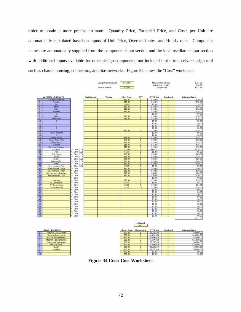
72
order to obtain a more precise estimate. Quantity Price, Extended Price, and Costs per Unit are
automatically calculated based on inputs of Unit Price, Overhead rates, and Hourly rates. Component
names are automatically supplied from the component input section and the local oscillator input section
with additional inputs available for other design components not included in the transceiver design tool
such as chassis housing, connectors, and bias networks. Figure 34 shows the “Cost” worksheet.
Figure 34 Cost: Cost Worksheet
Design Goal: Cost/Unit $750.00
Number of Units 10,000
MATERIAL - ESTIMATE Part Number Vendor Unit Price QTY QTY Price Overhead1 Connector/Inteface $10.00 1 $10.00 12 Amplifier $15.00 1 $15.00 13 Pad $5.00 1 $5.00 14 Mixer $10.00 1 $10.00 15 Filter $10.00 1 $10.00 16 Amplifier $15.00 1 $15.00 17 0 $0.00 18 Filter $10.00 1 $10.00 19 Attenuator $15.00 1 $15.00 110 0 $0.00 111 0 $0.00 112 0 $0.00 113 0 $0.00 114 0 $25.00 1 $25.00 115 Power Amplifier $0.00 116 0 $0.00 117 2 Way Hybrid $15.00 1 $15.00 118 Power Amp - Pair $45.00 2 $90.00 119 2 Way Hybrid $15.00 1 $15.00 120 Coupler $15.00 1 $15.00 121 Connector/Inteface $10.00 1 $10.00 122 Oscillator <-- Other (LO) $125.00 1 $125.00 123 Pad <-- Other (LO) $5.00 1 $5.00 124 Buffer Amp <-- Other (LO) $25.00 1 $25.00 125 Tripler <-- Other (LO) $25.00 1 $25.00 126 Divider <-- Other (LO) $25.00 1 $25.00 127 LO Amplifier <-- Other (LO) $25.00 1 $25.00 128 Filter <-- Other (LO) $10.00 1 $10.00 129 Line Loss and Pad <-- Other (LO) $5.00 1 $5.00 130 Bias Network - Amp <-- Other $10.00 2 $20.00 131 Bias Network - Atten <-- Other $10.00 1 $10.00 132 Bias Network - PwrAmp <-- Other $10.00 3 $30.00 133 Bias Networks - LO <-- Other $10.00 3 $30.00 134 <-- Other $0.00 135 Housing <-- Other $75.00 1 $75.00 136 IF Connectors <-- Other $5.00 1 $5.00 137 RF Connectors <-- Other $8.00 3 $24.00 138 DC Connectors <-- Other $1.00 18 $18.00 139 <-- Other $0.00 140 <-- Other $0.00 141 <-- Other $0.00 142 <-- Other $0.00 143 <-- Other $0.00 144 <-- Other $0.00 145 <-- Other $0.00 146 <-- Other $0.00 147 <-- Other $0.00 148 <-- Other $0.00 149 <-- Other $0.00 150 <-- Other $0.00 1
Hrs/Month160
LABOR - ESTIMATE Hourly Rate Manmonths QTY Price Overhead1 Program Management $50.00 1 $8,000.00 12 Systems Engineering $50.00 2 $16,000.00 13 Electrical Engineering $50.00 3 $24,000.00 14 Mechanical Engineering $50.00 2 $16,000.00 15 Specialty Engineering $50.00 1 $8,000.00 16 Manufacturing $50.00 2 $16,000.00 17 Quality $50.00 1 $8,000.00 18 Drafting $50.00 1 $8,000.00 19 $50.00 $0.00 110 $50.00 $0.00 1
$15.00$0.00
$10.00$15.00$0.00
$10.00
Extended Price
$15.00$5.00
$10.00
$10.00
$0.00$0.00$0.00
$25.00$0.00$0.00
$15.00$90.00$15.00$15.00$10.00
$125.00$5.00
$25.00$25.00$25.00$25.00$10.00$5.00
$20.00$10.00$30.00$30.00$0.00
$75.00$5.00
$24.00$18.00$0.00$0.00$0.00$0.00$0.00$0.00$0.00$0.00$0.00$0.00$0.00$0.00
$8,000.00
Extended Price$8,000.00
$16,000.00$24,000.00
$717.00
$16,000.00$8,000.00
$16,000.00
Material Cost per UnitLabor Cost per Unit
Cost per Unit
$717.00$10.40
$727.40
$8,000.00$0.00$0.00

73
5.10 Chart Data (and Graphs)
The “Chart Data” worksheet is used to capture the cumulative responses for graphing purposes.
Pre-set graphs are available but views are user dependent so additional detail will not be discussed here.

74
CHAPTER VI CONCLUSION
The inability to understand, analyze, and predict sources of variations in the design and
manufacturing of products will result in failures occurring during the production phase resulting in profit
lose and decreased customer satisfaction. The reduction of these variations in products such as state-of-
the-art transceivers to meet continuous customer demands of higher quality at reduced costs requires a
shift in traditional engineering design practices and decision-making processes. The design practices and
decision-making processes used today – nominal and worst-case design methodologies that only provide
a measure of design “goodness” – must be tossed away and replaced with statistical design methodologies
that allow informed decisions to be made based upon statistical information. Increased focus must be
placed on increasing engineering productivity during the early conceptual and detailed design phases of a
program by reducing a design’s sensitivity to component, environmental, and circuit variations and
thereby increasing design margins. The transceiver design tool presented here uses statistical design
methodologies and was designed as an aid to the systems engineer during the proposal, conceptual, and
early design phases of a program in developing variation insensitive designs.
These statistical design methodologies and transceiver design tool have been successfully used in
engineering design and product test applications. The transceiver design tool was used to achieve first-
pass yields of greater than 95% on three different sub-assemblies used in over 3,000 transceivers around
the world and to reduce standard transceiver design cycle times from eight months down to five months
and in one case down to 1.5 months with a savings of over $2,000,000. Statistical based decisions have
been used to reduce the amount of testing on products meeting requirements with sufficient margin and
save over $15,000,000. The application of this tool and the methodology behind it shows the benefits of
understanding the variability of designs early and their assembly processes along with the value of
reducing this variability whenever and wherever it is practical.

75
REFERENCES
Junkins, Jerry, “Texas Instruments Customer Satisfaction Through Total Quality – Management Perspective”. Harry, M. and Lawton, J, 1990, “Six Sigma Producibility Analysis and Process Optimization” pp. 1-3, 5-6 to 5-11
Ertas, A. and Jones, J., 1996, “The Engineering Design Process”, John Wiley & Sons, New York, p. 30.
Bhote, K., 2003, “The Power of Ultimate Six Sigma”, American Management Association, New York, p. 16-25.
Walpole, R. E., and Myers, R. H, 1978, “Probability and Statistics for Engineers and Scientists”, Macmillan, New York, Second Edition. Motorola University, 2002, (online). Available at: http://mu.motorola.com/
- Available at: http://mu.motorola.com/sixsigma.shtml - Available at: http://mu.motorola.com/history.shtml - Available at: http://mu.motorola.com/experience.shtml
Arnold, P., 1999, “Pursuing the Holy Grail”, MRO Today, (online).
Available at: http://www.mrotoday.com/mro/archives/Editorials/editJJ1999.htm American Statistical Association, Quality and Productivity Section, 2001, “Enabling Broad Application of Statistical Thinking”, Glossary of Statistical Terms, Quality Press, (online). Available at: http://web.utk.edu/~asaqp/thinking.html Waxer, C., 2003, “Six Sigma Costs and Savings”, iSixSigma LLC (online). Available at: http://www.isixsigma.com/library/content/c020729a.asp Norby, G. and Kollman, T., 2002, “Systems Engineering Principles”, Raytheon/Texas Tech ME-5354, p. 157. Decisioneering, 2003, (online). Available at: http://www.decisioneering.com/crystal_ball/index.html Decisioneering, 2000, “Crystal Ball 2000, User Manual” pp. 55 – 60, 122, 130-131, 232.

A-1
APPENDIX A SIMULATION REPORT – TYPICAL TRANSMITTER
Crystal Ball Report
Simulation started on 10/1/03 at
21:14:59
Simulation stopped on 10/1/03 at
21:18:05

A-2

A-3
Forecast: Gain (Cold) Cell: J11
Summary:Display Range is from 32.00 to 32.01 dBEntire Range is from 32.00 to 32.00 dBAfter 1,000 Trials, the Std. Error of the Mean is 0.00
Statistics: ValueTrials 1000Mean 32.00Median 32.00Mode ---Standard Deviation 0.00Variance 0.00Skewness 0.02Kurtosis 1.80Coeff. of Variability 0.00Range Minimum 32.00Range Maximum 32.00Range Width 0.01Mean Std. Error 0.00
Forecast: Gain (Cold) (cont'd) Cell: J11
Percentiles:
Percentile dB0% 32.00
10% 32.0020% 32.0030% 32.0040% 32.0050% 32.0060% 32.0070% 32.0080% 32.0090% 32.00
100% 32.00
End of Forecast
Frequency Chart
dB
.000
.005
.010
.015
.020
0
5
10
15
20
32.00 32.00 32.00 32.00 32.01
1,000 Trials 0 Outliers
Forecast: Gain (Cold)

A-4
Forecast: Gain (Room) Cell: K11
Summary:Display Range is from 32.00 to 32.01 dBEntire Range is from 32.00 to 32.00 dBAfter 1,000 Trials, the Std. Error of the Mean is 0.00
Statistics: ValueTrials 1000Mean 32.00Median 32.00Mode ---Standard Deviation 0.00Variance 0.00Skewness 0.02Kurtosis 1.82Coeff. of Variability 0.00Range Minimum 32.00Range Maximum 32.00Range Width 0.01Mean Std. Error 0.00
Forecast: Gain (Room) (cont'd) Cell: K11
Percentiles:
Percentile dB0% 32.00
10% 32.0020% 32.0030% 32.0040% 32.0050% 32.0060% 32.0070% 32.0080% 32.0090% 32.00
100% 32.00
End of Forecast
Frequency Chart
dB
.000
.005
.010
.015
.020
0
5
10
15
20
32.00 32.00 32.00 32.00 32.01
1,000 Trials 0 Outliers
Forecast: Gain (Room)

A-5
Forecast: Gain (Hot) Cell: L11
Summary:Display Range is from 31.95 to 32.01 dBEntire Range is from 31.42 to 32.00 dBAfter 1,000 Trials, the Std. Error of the Mean is 0.00
Statistics: ValueTrials 1000Mean 32.00Median 32.00Mode ---Standard Deviation 0.02Variance 0.00Skewness -27.66Kurtosis 825.04Coeff. of Variability 0.00Range Minimum 31.42Range Maximum 32.00Range Width 0.59Mean Std. Error 0.00
Forecast: Gain (Hot) (cont'd) Cell: L11
Percentiles:
Percentile dB0% 31.42
10% 32.0020% 32.0030% 32.0040% 32.0050% 32.0060% 32.0070% 32.0080% 32.0090% 32.00
100% 32.00
End of Forecast
Frequency Chart
dB
.000
.018
.036
.053
.071
0
17.75
35.5
53.25
71
31.95 31.96 31.98 31.99 32.01
1,000 Trials 4 Outliers
Forecast: Gain (Hot)

A-6
Forecast: Noise Figure (Cold) Cell: J12
Summary:Display Range is from 12.50 to 17.00 dBEntire Range is from 12.45 to 17.70 dBAfter 1,000 Trials, the Std. Error of the Mean is 0.03
Statistics: ValueTrials 1000Mean 14.67Median 14.64Mode ---Standard Deviation 0.82Variance 0.67Skewness 0.29Kurtosis 2.92Coeff. of Variability 0.06Range Minimum 12.45Range Maximum 17.70Range Width 5.24Mean Std. Error 0.03
Forecast: Noise Figure (Cold) (cont'd) Cell: J12
Percentiles:
Percentile dB0% 12.45
10% 13.6520% 13.9430% 14.1840% 14.4150% 14.6460% 14.8670% 15.0880% 15.3490% 15.79
100% 17.70
End of Forecast
Frequency Chart
dB
.000
.008
.016
.023
.031
0
7.75
15.5
23.25
31
12.50 13.63 14.75 15.88 17.00
1,000 Trials 5 Outliers
Forecast: Noise Figure (Cold)

A-7
Forecast: Noise Figure (Room) Cell: K12
Summary:Display Range is from 13.00 to 16.00 dBEntire Range is from 12.47 to 16.37 dBAfter 1,000 Trials, the Std. Error of the Mean is 0.02
Statistics: ValueTrials 1000Mean 14.47Median 14.45Mode ---Standard Deviation 0.56Variance 0.32Skewness 0.13Kurtosis 2.99Coeff. of Variability 0.04Range Minimum 12.47Range Maximum 16.37Range Width 3.90Mean Std. Error 0.02
Forecast: Noise Figure (Room) (cont'd) Cell: K12
Percentiles:
Percentile dB0% 12.47
10% 13.7520% 13.9930% 14.1640% 14.3050% 14.4560% 14.6170% 14.7780% 14.9590% 15.19
100% 16.37
End of Forecast
Frequency Chart
dB
.000
.007
.014
.021
.028
0
7
14
21
28
13.00 13.75 14.50 15.25 16.00
1,000 Trials 8 Outliers
Forecast: Noise Figure (Room)

A-8
Forecast: Noise Figure (Hot) Cell: L12
Summary:Display Range is from 14.00 to 17.50 dBEntire Range is from 13.70 to 17.29 dBAfter 1,000 Trials, the Std. Error of the Mean is 0.02
Statistics: ValueTrials 1000Mean 15.63Median 15.59Mode ---Standard Deviation 0.54Variance 0.30Skewness 0.13Kurtosis 2.94Coeff. of Variability 0.03Range Minimum 13.70Range Maximum 17.29Range Width 3.59Mean Std. Error 0.02
Forecast: Noise Figure (Hot) (cont'd) Cell: L12
Percentiles:
Percentile dB0% 13.70
10% 14.9220% 15.1930% 15.3340% 15.4650% 15.5960% 15.7470% 15.9180% 16.0990% 16.33
100% 17.29
End of Forecast
Frequency Chart
dB
.000
.008
.015
.023
.030
0
7.5
15
22.5
30
14.00 14.88 15.75 16.63 17.50
1,000 Trials 1 Outlier
Forecast: Noise Figure (Hot)

A-9
Forecast: Output Power / tone (Cold) Cell: J13
Summary:Display Range is from 15.00 to 15.01 dBmEntire Range is from 15.00 to 15.00 dBmAfter 1,000 Trials, the Std. Error of the Mean is 0.00
Statistics: ValueTrials 1000Mean 15.00Median 15.00Mode ---Standard Deviation 0.00Variance 0.00Skewness 0.02Kurtosis 1.81Coeff. of Variability 0.00Range Minimum 15.00Range Maximum 15.00Range Width 0.01Mean Std. Error 0.00
Forecast: Output Power / tone (Cold) (cont'd) Cell: J13
Percentiles:
Percentile dBm0% 15.00
10% 15.0020% 15.0030% 15.0040% 15.0050% 15.0060% 15.0070% 15.0080% 15.0090% 15.00
100% 15.00
End of Forecast
Frequency Chart
dBm
.000
.005
.010
.015
.020
0
5
10
15
20
15.00 15.00 15.00 15.00 15.01
1,000 Trials 0 Outliers
Forecast: Output Power / tone (Cold)

A-10
Forecast: Output Power / tone (Room) Cell: K13
Summary:Display Range is from 15.00 to 15.01 dBmEntire Range is from 15.00 to 15.00 dBmAfter 1,000 Trials, the Std. Error of the Mean is 0.00
Statistics: ValueTrials 1000Mean 15.00Median 15.00Mode ---Standard Deviation 0.00Variance 0.00Skewness 0.02Kurtosis 1.80Coeff. of Variability 0.00Range Minimum 15.00Range Maximum 15.00Range Width 0.01Mean Std. Error 0.00
Forecast: Output Power / tone (Room) (cont'd) Cell: K13
Percentiles:
Percentile dBm0% 15.00
10% 15.0020% 15.0030% 15.0040% 15.0050% 15.0060% 15.0070% 15.0080% 15.0090% 15.00
100% 15.00
End of Forecast
Frequency Chart
dBm
.000
.005
.010
.015
.020
0
5
10
15
20
15.00 15.00 15.00 15.00 15.01
1,000 Trials 0 Outliers
Forecast: Output Power / tone (Room)

A-11
Forecast: Output Power / tone (Hot Cell: L13
Summary:Display Range is from 14.94 to 15.01 dBmEntire Range is from 14.42 to 15.00 dBmAfter 1,000 Trials, the Std. Error of the Mean is 0.00
Statistics: ValueTrials 1000Mean 15.00Median 15.00Mode ---Standard Deviation 0.02Variance 0.00Skewness -27.66Kurtosis 825.04Coeff. of Variability 0.00Range Minimum 14.42Range Maximum 15.00Range Width 0.59Mean Std. Error 0.00
Forecast: Output Power / tone (Hot (cont'd) Cell: L13
Percentiles:
Percentile dBm0% 14.42
10% 15.0020% 15.0030% 15.0040% 15.0050% 15.0060% 15.0070% 15.0080% 15.0090% 15.00
100% 15.00
End of Forecast
Frequency Chart
dBm
.000
.020
.039
.059
.078
0
19.5
39
58.5
78
14.94 14.96 14.98 14.99 15.01
1,000 Trials 4 Outliers
Forecast: Output Power / tone (Hot

A-12
Forecast: Output IP3 (Cold) Cell: J15
Summary:Display Range is from 35.50 to 39.50 dBmEntire Range is from 35.46 to 39.74 dBmAfter 1,000 Trials, the Std. Error of the Mean is 0.02
Statistics: ValueTrials 1000Mean 37.62Median 37.62Mode ---Standard Deviation 0.72Variance 0.52Skewness -0.01Kurtosis 2.94Coeff. of Variability 0.02Range Minimum 35.46Range Maximum 39.74Range Width 4.28Mean Std. Error 0.02
Forecast: Output IP3 (Cold) (cont'd) Cell: J15
Percentiles:
Percentile dBm0% 35.46
10% 36.7120% 36.9930% 37.2540% 37.4350% 37.6260% 37.7970% 38.0180% 38.2590% 38.54
100% 39.74
End of Forecast
Frequency Chart
dBm
.000
.008
.016
.023
.031
0
7.75
15.5
23.25
31
35.50 36.50 37.50 38.50 39.50
1,000 Trials 7 Outliers
Forecast: Output IP3 (Cold)

A-13
Forecast: Output IP3 (Room) Cell: K15
Summary:Display Range is from 34.50 to 38.50 dBmEntire Range is from 34.35 to 38.69 dBmAfter 1,000 Trials, the Std. Error of the Mean is 0.02
Statistics: ValueTrials 1000Mean 36.47Median 36.47Mode ---Standard Deviation 0.70Variance 0.49Skewness 0.00Kurtosis 2.90Coeff. of Variability 0.02Range Minimum 34.35Range Maximum 38.69Range Width 4.34Mean Std. Error 0.02
Forecast: Output IP3 (Room) (cont'd) Cell: K15
Percentiles:
Percentile dBm0% 34.35
10% 35.5720% 35.8530% 36.0840% 36.2950% 36.4760% 36.6770% 36.8480% 37.0590% 37.39
100% 38.69
End of Forecast
Frequency Chart
dBm
.000
.007
.015
.022
.029
0
7.25
14.5
21.75
29
34.50 35.50 36.50 37.50 38.50
1,000 Trials 5 Outliers
Forecast: Output IP3 (Room)

A-14
Forecast: Output IP3 (Hot) Cell: L15
Summary:Display Range is from 34.00 to 38.00 dBmEntire Range is from 33.78 to 38.34 dBmAfter 1,000 Trials, the Std. Error of the Mean is 0.02
Statistics: ValueTrials 1000Mean 36.00Median 36.01Mode ---Standard Deviation 0.76Variance 0.58Skewness -0.01Kurtosis 2.89Coeff. of Variability 0.02Range Minimum 33.78Range Maximum 38.34Range Width 4.56Mean Std. Error 0.02
Forecast: Output IP3 (Hot) (cont'd) Cell: L15
Percentiles:
Percentile dBm0% 33.78
10% 35.0520% 35.3430% 35.5940% 35.8250% 36.0160% 36.1970% 36.4280% 36.6590% 36.98
100% 38.34
End of Forecast
Frequency Chart
dBm
.000
.007
.013
.020
.026
0
6.5
13
19.5
26
34.00 35.00 36.00 37.00 38.00
1,000 Trials 9 Outliers
Forecast: Output IP3 (Hot)

A-15
Forecast: Input IP3 (Cold) Cell: J16
Summary:Display Range is from 3.50 to 7.50 dBmEntire Range is from 3.46 to 7.74 dBmAfter 1,000 Trials, the Std. Error of the Mean is 0.02
Statistics: ValueTrials 1000Mean 5.62Median 5.61Mode ---Standard Deviation 0.72Variance 0.52Skewness -0.01Kurtosis 2.94Coeff. of Variability 0.13Range Minimum 3.46Range Maximum 7.74Range Width 4.28Mean Std. Error 0.02
Forecast: Input IP3 (Cold) (cont'd) Cell: J16
Percentiles:
Percentile dBm0% 3.46
10% 4.7120% 4.9930% 5.2540% 5.4350% 5.6160% 5.8070% 6.0180% 6.2590% 6.53
100% 7.74
End of Forecast
Frequency Chart
dBm
.000
.007
.015
.022
.029
0
7.25
14.5
21.75
29
3.50 4.50 5.50 6.50 7.50
1,000 Trials 7 Outliers
Forecast: Input IP3 (Cold)

A-16
Forecast: Input IP3 (Room) Cell: K16
Summary:Display Range is from 2.50 to 6.50 dBmEntire Range is from 2.35 to 6.69 dBmAfter 1,000 Trials, the Std. Error of the Mean is 0.02
Statistics: ValueTrials 1000Mean 4.47Median 4.48Mode ---Standard Deviation 0.70Variance 0.49Skewness 0.00Kurtosis 2.90Coeff. of Variability 0.16Range Minimum 2.35Range Maximum 6.69Range Width 4.34Mean Std. Error 0.02
Forecast: Input IP3 (Room) (cont'd) Cell: K16
Percentiles:
Percentile dBm0% 2.35
10% 3.5720% 3.8430% 4.0840% 4.2950% 4.4860% 4.6770% 4.8380% 5.0590% 5.39
100% 6.69
End of Forecast
Frequency Chart
dBm
.000
.007
.015
.022
.029
0
7.25
14.5
21.75
29
2.50 3.50 4.50 5.50 6.50
1,000 Trials 5 Outliers
Forecast: Input IP3 (Room)

A-17
Forecast: Input IP3 (Hot) Cell: L16
Summary:Display Range is from 2.00 to 6.00 dBmEntire Range is from 1.78 to 6.34 dBmAfter 1,000 Trials, the Std. Error of the Mean is 0.02
Statistics: ValueTrials 1000Mean 4.00Median 4.01Mode ---Standard Deviation 0.76Variance 0.58Skewness -0.01Kurtosis 2.89Coeff. of Variability 0.19Range Minimum 1.78Range Maximum 6.34Range Width 4.55Mean Std. Error 0.02
Forecast: Input IP3 (Hot) (cont'd) Cell: L16
Percentiles:
Percentile dBm0% 1.78
10% 3.0520% 3.3430% 3.5940% 3.8150% 4.0160% 4.1970% 4.4280% 4.6590% 4.98
100% 6.34
End of Forecast
Frequency Chart
dBm
.000
.007
.014
.020
.027
0
6.75
13.5
20.25
27
2.00 3.00 4.00 5.00 6.00
1,000 Trials 9 Outliers
Forecast: Input IP3 (Hot)

A-18
Forecast: IMR Level (Cold) Cell: J17
Summary:Display Range is from -49.00 to -41.00 dBcEntire Range is from -49.48 to -40.92 dBcAfter 1,000 Trials, the Std. Error of the Mean is 0.05
Statistics: ValueTrials 1000Mean -45.24Median -45.24Mode ---Standard Deviation 1.44Variance 2.07Skewness 0.01Kurtosis 2.94Coeff. of Variability -0.03Range Minimum -49.48Range Maximum -40.92Range Width 8.57Mean Std. Error 0.05
Forecast: IMR Level (Cold) (cont'd) Cell: J17
Percentiles:
Percentile dBc0% -49.48
10% -47.0720% -46.5130% -46.0240% -45.6050% -45.2460% -44.8870% -44.5080% -43.9990% -43.43
100% -40.92
End of Forecast
Frequency Chart
dBc
.000
.007
.015
.022
.029
0
7.25
14.5
21.75
29
-49.00 -47.00 -45.00 -43.00 -41.00
1,000 Trials 7 Outliers
Forecast: IMR Level (Cold)

A-19
Forecast: IMR Level (Room) Cell: K17
Summary:Display Range is from -47.00 to -39.00 dBcEntire Range is from -47.39 to -38.71 dBcAfter 1,000 Trials, the Std. Error of the Mean is 0.04
Statistics: ValueTrials 1000Mean -42.94Median -42.96Mode ---Standard Deviation 1.40Variance 1.95Skewness 0.00Kurtosis 2.90Coeff. of Variability -0.03Range Minimum -47.39Range Maximum -38.71Range Width 8.68Mean Std. Error 0.04
Forecast: IMR Level (Room) (cont'd) Cell: K17
Percentiles:
Percentile dBc0% -47.39
10% -44.7920% -44.1130% -43.6740% -43.3450% -42.9660% -42.5870% -42.1780% -41.6990% -41.15
100% -38.71
End of Forecast
Frequency Chart
dBc
.000
.007
.015
.022
.029
0
7.25
14.5
21.75
29
-47.00 -45.00 -43.00 -41.00 -39.00
1,000 Trials 5 Outliers
Forecast: IMR Level (Room)

A-20
Forecast: IMR Level (Hot) Cell: L17
Summary:Display Range is from -46.00 to -38.00 dBcEntire Range is from -46.68 to -37.57 dBcAfter 1,000 Trials, the Std. Error of the Mean is 0.05
Statistics: ValueTrials 1000Mean -42.01Median -42.02Mode ---Standard Deviation 1.53Variance 2.33Skewness 0.01Kurtosis 2.89Coeff. of Variability -0.04Range Minimum -46.68Range Maximum -37.57Range Width 9.11Mean Std. Error 0.05
Forecast: IMR Level (Hot) (cont'd) Cell: L17
Percentiles:
Percentile dBc0% -46.68
10% -43.9720% -43.3230% -42.8540% -42.3950% -42.0260% -41.6370% -41.1980% -40.7190% -40.10
100% -37.57
End of Forecast
Frequency Chart
dBc
.000
.007
.014
.020
.027
0
6.75
13.5
20.25
27
-46.00 -44.00 -42.00 -40.00 -38.00
1,000 Trials 9 Outliers
Forecast: IMR Level (Hot)

A-21
Forecast: Noise Power (Cold) Cell: J18
Summary:Display Range is from -129.50 to -125.00 dBm/BWEntire Range is from -129.52 to -124.28 dBm/BWAfter 1,000 Trials, the Std. Error of the Mean is 0.03
Statistics: ValueTrials 1000Mean -127.31Median -127.33Mode ---Standard Deviation 0.82Variance 0.67Skewness 0.29Kurtosis 2.92Coeff. of Variability -0.01Range Minimum -129.52Range Maximum -124.28Range Width 5.24Mean Std. Error 0.03
Forecast: Noise Power (Cold) (cont'd) Cell: J18
Percentiles:
Percentile dBm/BW0% -129.52
10% -128.3220% -128.0330% -127.7940% -127.5650% -127.3360% -127.1270% -126.9080% -126.6390% -126.19
100% -124.28
End of Forecast
Frequency Chart
dBm/BW
.000
.007
.015
.022
.029
0
7.25
14.5
21.75
29
-129.50 -128.38 -127.25 -126.13 -125.00
1,000 Trials 5 Outliers
Forecast: Noise Power (Cold)

A-22
Forecast: Noise Power (Room) Cell: K18
Summary:Display Range is from -129.00 to -126.00 dBm/BWEntire Range is from -129.51 to -125.60 dBm/BWAfter 1,000 Trials, the Std. Error of the Mean is 0.02
Statistics: ValueTrials 1000Mean -127.51Median -127.53Mode ---Standard Deviation 0.56Variance 0.32Skewness 0.13Kurtosis 2.99Coeff. of Variability 0.00Range Minimum -129.51Range Maximum -125.60Range Width 3.90Mean Std. Error 0.02
Forecast: Noise Power (Room) (cont'd) Cell: K18
Percentiles:
Percentile dBm/BW0% -129.51
10% -128.2320% -127.9930% -127.8240% -127.6850% -127.5360% -127.3770% -127.2180% -127.0390% -126.79
100% -125.60
End of Forecast
Frequency Chart
dBm/BW
.000
.006
.013
.019
.025
0
6.25
12.5
18.75
25
-129.00 -128.25 -127.50 -126.75 -126.00
1,000 Trials 8 Outliers
Forecast: Noise Power (Room)

A-23
Forecast: Noise Power (Hot) Cell: L18
Summary:Display Range is from -128.00 to -124.50 dBm/BWEntire Range is from -128.27 to -124.68 dBm/BWAfter 1,000 Trials, the Std. Error of the Mean is 0.02
Statistics: ValueTrials 1000Mean -126.35Median -126.38Mode ---Standard Deviation 0.54Variance 0.30Skewness 0.13Kurtosis 2.94Coeff. of Variability 0.00Range Minimum -128.27Range Maximum -124.68Range Width 3.59Mean Std. Error 0.02
Forecast: Noise Power (Hot) (cont'd) Cell: L18
Percentiles:
Percentile dBm/BW0% -128.27
10% -127.0620% -126.7930% -126.6540% -126.5250% -126.3860% -126.2470% -126.0780% -125.8990% -125.65
100% -124.68
End of Forecast
Frequency Chart
dBm/BW
.000
.008
.016
.024
.032
0
8
16
24
32
-128.00 -127.13 -126.25 -125.38 -124.50
1,000 Trials 1 Outlier
Forecast: Noise Power (Hot)

A-24
Forecast: S/N Ratio (Cold) Cell: J19
Summary:Display Range is from 140.00 to 144.50 Entire Range is from 139.28 to 144.52 After 1,000 Trials, the Std. Error of the Mean is 0.03
Statistics: ValueTrials 1000Mean 142.31Median 142.33Mode ---Standard Deviation 0.82Variance 0.67Skewness -0.29Kurtosis 2.92Coeff. of Variability 0.01Range Minimum 139.28Range Maximum 144.52Range Width 5.24Mean Std. Error 0.03
Forecast: S/N Ratio (Cold) (cont'd) Cell: J19
Percentiles:
Percentile Value0% 139.28
10% 141.1820% 141.6330% 141.8940% 142.1150% 142.3360% 142.5670% 142.7980% 143.0390% 143.32
100% 144.52
End of Forecast
Frequency Chart
.000
.008
.015
.023
.030
0
7.5
15
22.5
30
140.00 141.13 142.25 143.38 144.50
1,000 Trials 5 Outliers
Forecast: S/N Ratio (Cold)

A-25
Forecast: S/N Ratio (Room) Cell: K19
Summary:Display Range is from 141.00 to 144.00 Entire Range is from 140.60 to 144.51 After 1,000 Trials, the Std. Error of the Mean is 0.02
Statistics: ValueTrials 1000Mean 142.51Median 142.52Mode ---Standard Deviation 0.56Variance 0.32Skewness -0.13Kurtosis 2.99Coeff. of Variability 0.00Range Minimum 140.60Range Maximum 144.51Range Width 3.90Mean Std. Error 0.02
Forecast: S/N Ratio (Room) (cont'd) Cell: K19
Percentiles:
Percentile Value0% 140.60
10% 141.7920% 142.0330% 142.2040% 142.3750% 142.5260% 142.6770% 142.8280% 142.9990% 143.23
100% 144.51
End of Forecast
Frequency Chart
.000
.006
.013
.019
.025
0
6.25
12.5
18.75
25
141.00 141.75 142.50 143.25 144.00
1,000 Trials 8 Outliers
Forecast: S/N Ratio (Room)

A-26
Forecast: S/N Ratio (Hot) Cell: L19
Summary:Display Range is from 139.50 to 143.00 Entire Range is from 139.68 to 143.28 After 1,000 Trials, the Std. Error of the Mean is 0.02
Statistics: ValueTrials 1000Mean 141.35Median 141.38Mode ---Standard Deviation 0.54Variance 0.30Skewness -0.13Kurtosis 2.94Coeff. of Variability 0.00Range Minimum 139.68Range Maximum 143.28Range Width 3.59Mean Std. Error 0.02
Forecast: S/N Ratio (Hot) (cont'd) Cell: L19
Percentiles:
Percentile Value0% 139.68
10% 140.6420% 140.8830% 141.0740% 141.2450% 141.3860% 141.5270% 141.6480% 141.7990% 142.05
100% 143.28
End of Forecast
Frequency Chart
.000
.008
.017
.025
.033
0
8.25
16.5
24.75
33
139.50 140.38 141.25 142.13 143.00
1,000 Trials 1 Outlier
Forecast: S/N Ratio (Hot)


![A Contemporary Design Tool [TOC] Embedded Systems](https://img.dokumen.tips/doc/110x75/577cc12a1a28aba7119270b7/a-contemporary-design-tool-toc-embedded-systems.jpg)