Embed Size (px)
Citation preview
Design and Implementation of a Constant Envelope OFDM Waveform in a Software Defined
Radio Platform
Amos Vershima Ajo Jr.
Thesis submitted to the faculty of the Virginia Polytechnic Institute and State University in
partial fulfillment of the requirements for the degree of
Master of Science
in
Electrical Engineering
Carl B. Dietrich, Chair
A. A. (Louis) Beex, Chair
Allen B. MacKenzie
May 5, 2016
Blacksburg, Virginia
Keywords: OFDM, Constant Envelope OFDM, Peak-to-Average Power Ratio, Software Defined
Radio, GNU Radio

Design and Implementation of a Constant Envelope OFDM Waveform in a Software Defined
Radio Platform
Amos Vershima Ajo Jr.
ABSTRACT
This thesis examines the high peak-to-average-power ratio (PAPR) problem of OFDM and other
spectrally-efficient multicarrier modulation schemes, specifically their stringent requirements for
highly linear, power-inefficient amplification. The thesis then presents a most intriguing answer
to the PAPR-problem in the form of a constant-envelope OFDM (CE-OFDM) waveform, a
waveform which employs phase modulation to transform the high-PAPR OFDM signal into a
constant envelope signal, like FSK or GMSK, which can be amplified with non-linear power
amplifiers at near saturation levels of efficiency. A brief analytical description of CE-OFDM and
its suboptimal receiver architecture is provided in order to define and analyze the key parameters
of the waveform and their performance impacts.
The primary contribution of this thesis is a highly tunable software-defined radio (SDR)
implementation of the waveform which enables rapid-prototyping and testing of CE-OFDM
systems. The digital baseband processing of the waveform is executed on a general purpose
processor (GPP) in the Ubuntu 14.04 Linux operating system, and programmed using the GNU
Radio SDR software framework with a mixture of Python and C++ routines. A detailed description
of the software implementation is provided, and baseband simulations of the SDR CE-OFDM
receiver in additive white Gaussian noise (AWGN) validate the performance of the implemented
signal processing.
A fully-functional CE-OFDM radio system is proposed in which GPPs executing the software
defined transmitter and receiver routines are interfaced with Ettus Universal Software Radio
Peripheral (USRP) transceiver front ends. A software ‘test bench’ is created to enable rapid
configuration and testing of the CE-OFDM waveform over all permutations of its parameters, over
both simulated and physical RF channels, to draw deeper insights into the characteristics of the
waveform and the necessary design considerations and improvements for further development and
deployment of CE-OFDM systems.
Design and Implementation of a Constant Envelope OFDM Waveform in a Software Defined
Radio Platform
Amos Vershima Ajo Jr.
GENERAL AUDIENCE ABSTRACT
Orthogonal Frequency Division Multiplexing (OFDM) is a modulation scheme which has become
virtually ubiquitous in the world of wireless communications; from the radio frequency (RF)
signals transmitted to and from our Wi-Fi routers, to the RF signals transmitted to and from our
mobile carrier’s LTE cellular towers, the transmission and reception of OFDM signals has become
nearly essential to our daily life. OFDM’s virtues include its outstanding versatility and ability to
deliver high-data rate communications over harsh mobile radio channels, but its primary downfall
is the demand it makes for significant energy waste upon amplification. A novel modulation
scheme called constant-envelope OFDM (CE-OFDM) is a unique solution power inefficiency
problem of traditional OFDM, as it offers nearly optimal levels of power efficiency at the power
amplifier (PA).
In this thesis, CE-OFDM is described qualitatively and analytically to, respectively, motivate an
understanding of the waveform’s advantages over traditional OFDM, and detail an implementation
of a CE-OFDM transmitter and receiver in which the waveform’s key performance-affecting
parameters are easily tunable in software. Using software-defined radio (SDR), a paradigm of radio
design in which a significant amount of dedicated circuitry in a radio is replaced with
programmable hardware, a fully-functional, highly configurable, CE-OFDM radio system was
implemented. This system forms a platform which can simultaneously simulate the performance
of CE-OFDM in a purely-software environment, where its various nuances and performance over
a variety of radio environments can be analyzed, and also interface with SDR RF hardware to
implement real CE-OFDM radio links. The promise of this work is to enhance the knowledge of
CE-OFDM waveform performance and behavior, shorten the lifecycle between the simulation and
the implementation of CE-OFDM systems, and promote further research and development of CE-
OFDM systems for a greener telecommunications industry.

iv
ACKNOWLEDGEMENTS
I would like to give my deepest thanks to my advisor and committee chair, Dr. Dietrich for his
mentorship, support, assistance and patience during the development of this thesis and throughout
my graduate education at Virginia Tech. I would also like to express my gratitude to the members
of my thesis committee, Dr. Beex and Dr. MacKenzie for offering their time, guidance, and critical
insights.
I would like to especially thank Dr. Dietrich and Dr. Beex for inspiring me to pursue my graduate
education at Virginia Tech, during my NSF Research Experience for Undergraduates (REU)
Internship in the summer of 2013.
I would like express my deepest gratitude to Joe Molnar of the Naval Research Laboratory for
providing me the opportunity to begin my research, and I would also like to thank Frank Fu and
Andrew Robertson for their guidance and mentorship.
Finally but not the least, I would like to express my deepest appreciation for my Mom and Dad
who have offered me unending love, support, and encouragement throughout my entire life, and
vitally so during my graduate studies. I dedicate this thesis to them.
v
TABLE OF CONTENTS
Abstract .......................................................................................................................................... ii
Acknowledgements ...................................................................................................................... iv
Table of Contents ...........................................................................................................................v
Glossary of Terms ...................................................................................................................... viii
List of Figures ............................................................................................................................... xi
1 Introduction ............................................................................................................................1
1.1 Motivation ........................................................................................................................1
1.2 Contribution .....................................................................................................................2
1.3 Organization .....................................................................................................................3
2 Software-Defined Radio Background ..................................................................................4
2.1 SDR Concept ...................................................................................................................4
2.2 SDR Hardware .................................................................................................................5
2.2.1 SDR Radio Frequency Front-End ................................................................................5
2.2.2 SDR Digital Front-End ................................................................................................6
2.2.3 SDR Baseband Digital Processor.................................................................................6
2.3 SDR Software ..................................................................................................................7
2.4 Proposed SDR Platform ...................................................................................................7
3 Orthogonal Frequency-Division Multiplexing Background ..............................................9
3.1 Multipath Fading Phenomena ..........................................................................................9
3.1.1 Time-Domain Representation of a Multipath Channel ..............................................10
3.1.2 Frequency-Domain Representation of a Multipath Channel .....................................11
3.1.3 Impairments of Multipath on Single-Carrier Modulation ..........................................11
3.2 OFDM in Multipath Channels .......................................................................................13
3.2.1 Frequency-Selective Fading Immunity of OFDM .....................................................14
3.2.2 Inter-Symbol-Interference Immunity of OFDM ........................................................14
3.3 Analytical Description of OFDM ..................................................................................15
3.3.1 Digital Implementation of OFDM .............................................................................16
3.4 Benefits of OFDM .........................................................................................................18
4 The Problem of Peak-to-Average Power Ratio in OFDM ...............................................20

vi
4.1 PAPR Statistics of OFDM .............................................................................................20
4.2 Power Amplification of High-PAPR OFDM .................................................................21
4.2.1 Power Amplifier Basics .............................................................................................22
4.2.2 OFDM Linearity Requirement ...................................................................................26
4.3 Power Consumption Considerations ..............................................................................29
5 Constant-Envelope OFDM ..................................................................................................31
5.1 CE-OFDM Concept .......................................................................................................31
5.2 CE-OFDM Signal Definition .........................................................................................32
5.3 CE-OFDM Waveform Parameters .................................................................................34
5.3.1 Symbol Mapping {𝐼𝑖, 𝑘} : ...........................................................................................34
5.3.2 Subcarrier Set {𝑞𝑘(𝑡)}: ..............................................................................................34
5.3.3 Normalization Constant 𝐶𝑛: ......................................................................................36
5.3.4 Modulation Index 2𝜋ℎ: ..............................................................................................36
5.3.5 Memory Phases 𝜃𝑖: ....................................................................................................36
5.4 CE-OFDM Discrete-Domain Processing .......................................................................37
5.5 CE-OFDM Performance Consideration .........................................................................38
5.5.1 Spectral Analysis .......................................................................................................39
5.5.2 The Sub-Optimal CE-OFDM Receiver .....................................................................41
5.6 Critical Performance and Design Considerations ..........................................................44
5.6.1 The Challenges of CE-OFDM ...................................................................................44
5.6.2 The Strengths of CE-OFDM ......................................................................................47
5.7 Nonlinear Power Amplification of CE-OFDM..............................................................48
6 SDR Implementation of CE-OFDM Waveform................................................................50
6.1 GNU Radio SDR Development .....................................................................................50
6.1.1 Signal Processing Blocks ...........................................................................................50
6.1.2 GNU Radio Scheduler ...............................................................................................51
6.1.3 Python Programmatic Interface .................................................................................51
6.1.4 GNU Radio Companion Graphical Interface .............................................................51
6.1.5 Creating Custom GNU Radio Blocks ........................................................................51
6.2 CE-OFDM Transmitter Implementation........................................................................53
6.3 CE-OFDM Receiver Implementation ............................................................................55
vii
7 Simulation Methodology andd Resultss .............................................................................57
7.1 Simulation Methodology ...............................................................................................57
7.2 Simulation Results .........................................................................................................59
8 Conclusions ...........................................................................................................................66
8.1 Further Research ............................................................................................................66
8.1.1 Extending Waveform Implementation .......................................................................66
8.1.2 Extending Simulation and Analysis ...........................................................................66
8.1.3 RF Testing ..................................................................................................................67
8.1.4 Improving Computational Efficiency ........................................................................67
8.1.5 Cognitive Radio Integration .......................................................................................67
9 References .............................................................................................................................68
viii
GLOSSARY OF TERMS
3GPP . . . . . . . . . 3rd Generation Partnership Project
ACI . . . . . . . . . . Adjacent Channel Interference
ADC. . . . . . . . . . Analog to Digital Converter
AM . . . . . . . . . . . Amplitude Modulation
AM-AM . . . . . . . Amplitude-to-Amplitude Transfer Function
AWGN ………… Additive White Gaussian Noise
BER …………… Bit Error Rate
BPSK . . . . . . . . . Binary Phase-Shift Keying
C++ ……………. C-Plus-Plus, programming language
CCDF . . . . . . . . . Complimentary Cumulative Distribution Function
CDM . . . . . . . . . Code Division Multiplexing
CNR . . . . . . . . . . Carrier-to-Noise Ratio
CP. . . . . . . . . . . . Cyclic Prefix
CPU. . . . . . . . . . . Central Processing Unit
CR. . . . . . . . . . . Cyclic Redundancy Check
DAC . . . . . . . . . Digital to Analog Converter
DC . . . . . . . . . . . Direct Current
DDC . . . . . . . . . . Digital Downconverter
DFT…………….. Discrete Fourier Transform
DSL ……………. Digital Subscriber Line
DSP . . . . . . . . . . . Digital Signal Processor
DUC . . . . . . . . . . Digital Upconverter
EER . . . . . . . . . . Envelope Elimination and Restoration
EM . . . . . . . . . . . . Electromagnetic Wave
FDM . . . . . . . . . Frequency-Division Multiplexing
FEC……………. Forward Error Correction
FFT . . . . . . . . . . Fast Fourier Transform
FIR . . . . . . . . . . . Finite-Impulse Response
FM . . . . . . . . . . . Frequency Modulation
ix
FOBP . . . . . . . . . Fractional Out of Band Power
FPGA . . . . . . . . . Field-Programmable Gate Array
FSM . . . . . . . . . . Finite State Machine
GHz……………. Gigahertz (1000 MHz)
GNU . . . . . . . . . . “GNU’s Not UNIX” Open-Source Software System
GPP . . . . . . . . . . . General Purpose Processor
GRC . . . . . . . . . . GNU Radio Companion
GUI . . . . . . . . . . Graphical User Interface
i.i.d. . . . . . . . . . . Independent and Identically Distributed
IBO . . . . . . . . . . Input-Power Backoff
ICI . . . . . . . . . . Inter-Carrier Interference
IDFT . . . . . . . . . Inverse Discrete Fourier Transform
IEEE. . . . . . . . . Institute of Electrical and Electronics Engineers
IF . . . . . . . . . . . Intermediate Frequency
IFFT . . . . . . . . . . Inverse Fast Fourier Transform
IIP3 . . . . . . . . . . Third-Order Intercept Point
IIR . . . . . . . . . . . Infinite-Impulse Response
IMD . . . . . . . . . . Intermodulation Distortion
ISM . . . . . . . . . . Industrial, Scientific and Medical
kHz . . . . . . . . . . Kilohertz (1000 Hz)
LAN. . . . . . . . . . Local Area Network
LINC . . . . . . . . . Linear Amplification in Nonlinear Components
LTE . . . . . . . . . . . 3GPP Long Term Evolution
MAC. . . . . . . . . . Media Access Control
MHz…………… Megahertz (1000 kHz)
ML. . . . . . . . . . . Maximum Likelihood
OBO . . . . . . . . . . Output-Power Backoff
OFDM . . . . . . . Orthogonal Frequency-Division Multiplexing
OOP …………… Object Oriented Programming
PAPR………… Peak-to-Average Power Ratio
PC. . . . . . . . . . . . Personal Computer
x
PDF…………… Probability Density Function
PN . . . . . . . . . . . Pseudorandom Noise
PPM ………….. Parts Per Million
PSD . . . . . . . . . . Power Spectral Density
PSK . . . . . . . . . . Phase-Shift Keying
QAM . . . . . . . . . Quadrature Amplitude Modulation
QPSK . . . . . . . . Quadrature Phase-Shift Keying
RAM. . . . . . . . . Random Access Memory
RF. . . . . . . . . . . Radio Frequency
RMS…………. Root Mean Square
SC-FDMA. . . . . Single Carrier Frequency Division Multiple Access
SDR . . . . . . . . . . Software Defined Radio
SER…………. . Symbol Error Rate
SNR . . . . . . . . . . Signal-to-Noise Ratio
SWIG. . . . . . . . . Simplified Wrapper and Interface Generator
USB . . . . . . . . . . Universal Serial Bus
USRP . . . . . . . . . Universal Software Radio Peripheral
USRP N210 . . . . Universal Software Radio Peripheral Network-Series Model 210
VCO . . . . . . . . . . Voltage-Controlled Oscillator
Wi-Fi . . . . . . . . . 802.11 Wireless Local Area Network
WiMAX . . . . . . . Worldwide interoperability for Microwave Access
WLAN . . . . . . . . Wireless Local Area Network
XML . . . . . . . . . . Extensible Markup Language
xi
LIST OF FIGURES
Figure 2.1: SDR Concept .............................................................................................................. 4
Figure 2.2: General SDR Architecture .......................................................................................... 5
Figure 2.3: SDR System w/ USRP and GNU Radio .................................................................... 7
Figure 3.1: Multipath Signal Propagation ..................................................................................... 9
Figure 3.2: Multipath Channel Time-Domain Impulse Response .............................................. 10
Figure 3.3: Multipath Channel Frequency-Domain Response ................................................... 11
Figure 3.4: Inter-Symbol Interference on Short Symbols ........................................................... 12
Figure 3.5: Single Carrier Modulation …………………………………………………………13
Figure 3.6: Multi-Carrier Modulation ………………………………………………………….13
Figure 3.7: OFDM Modulation …………………………………………………………………14
Figure 3.8: Subchannelization of Wideband Multipath Channel ................................................ 14
Figure 3.9: ISI Compensation with Long Symbols .................................................................... 15
Figure 3.10: ISI Elimination w/ Cyclic Prefix ............................................................................ 15
Figure 3.11: OFDM Transmitter Block Diagram ....................................................................... 17
Figure 3.12: OFDM Receiver Block Diagram .............................................................................. 17
Figure 4.1: Instantaneous OFDM Signal Power over Symbol Period ........................................ 20
Figure 4.2: PA AM/AM Transfer Function ................................................................................ 23
Figure 4.3: PA Simple Diagram ………………………………………………………………...23
Figure 4.4: Effect of Operation Region on Drain Efficiency ...................................................... 24
Figure 4.5: Linearity-Efficiency Tradeoff among Class-C, B, and A PAs ................................. 26
Figure 4.6a: Nonlinear Amplification of OFDM ………………………………………………...27
Figure 4.6b: Linear Amplification of OFDM ………………………………………………........27
Figure 4.6c: Linear Amplification of OFDM with IBO ………………………………………....27
Figure 5.1: CE-OFDM Envelope vs. OFDM Envelope .............................................................. 31
Figure 5.2: Instantaneous Power of CE-OFDM vs OFDM ........................................................ 32
Figure 5.3: Simplified CE-OFDM Block Diagram..................................................................... 33
Figure 5.4: Inter-Symbol Continuity for Sine and Cosine Subcarriers ....................................... 35
Figure 5.5: Memory Phase Continuity after Cyclic Prefixing .................................................... 37
xii
Figure 5.6: CE-OFDM Transmitter Block Diagram ................................................................. 38
Figure 5.7: CE-OFDM Power Spectral Density Estimate FOBP ………………………….….40
Figure 5.8: Suboptimal CE-OFDM Receiver Block Diagram .................................................. 41
Figure 5.9: CE-OFDM Symbol Error Rate vs SNR vs various 2πh ........................................ 44
Figure 5.10: Phase Excursions of CE-OFDM vs h ..................................................................... 45
Figure 5.11a: Class C Nonlinear Amplification of CE-OFDM …………………………………49
Figure 5.11b: Class A Linear Amplification of OFDM …………………………………………49
Figure 6.1: GNU Radio Block Inheritance ................................................................................ 52
Figure 6.2: Graphical Interface of CE-OFDM Transmitter Block ............................................. 53
Figure 6.3: Transmitter Frame Structure Diagram ..................................................................... 54
Figure 6.4: Hierarchical Diagram of CE-OFDM Receiver ......................................................... 55
Figure 6.5: Graphical Interface of CE-OFDM Receiver ............................................................ 56
Figure 7.1: GNU Radio Simulation Flowgraph .......................................................................... 57
Figure 7.2: Python CE-OFDM Simulation Excerpt .................................................................... 59
Figure 7.3: 8-PAM, N=32, os factor=8 ....................................................................................... 61
Figure 7.4: 16-PAM, N=32, os factor=8 ..................................................................................... 62
Figure 7.5: 32-PAM, N=32, os factor=8 ..................................................................................... 63
Figure 7.6: 64-PAM, N=32, os factor=8 ..................................................................................... 64
Figure 8.1: GNU Radio Flowgraphs of RF CE-OFDM System ................................................. 67
1
1 INTRODUCTION
1.1 Motivation
Orthogonal Frequency Division Multiplexing (OFDM) is a multi-carrier modulation scheme
which has become virtually indispensable in the world of wireless communications. OFDM has
been the physical layer backbone and key enabler for the development of some our most important
wireless protocols, from the IEEE 802.11 standards for Wi-Fi to both the 3GPP Long Term
Evolution (LTE) and IEEE 802.16 Wi-MAX standards for 4G cellular communications. The
mathematical properties of OFDM make it a proverbial "Swiss army knife" for tackling some of
the most constraining challenges of wireless radio communications, particularly in enabling high
data rate communications over harsh mobile channels.
The multi-carrier nature of OFDM provides the modulation an inherent resilience to the frequency-
selective fading effects characteristic of broadband multipath radio channels, far surpassing the
multipath performance of its single-carrier (SC) modulation rivals. OFDM effectively reduces the
impact of a broadband multipath channel to that of several narrowband, single-path subchannels –
each requiring minimal, single-tap, equalization to compensate for multipath fading across the full
signal bandwidth. The orthogonality of OFDM subcarriers enables the modulation to utilize
bandwidth with greater efficiency, higher throughput and capacity than the traditional Frequency
Division Multiplexing (FDM) techniques. OFDM also leverages this subcarrier orthogonality to
enable such ingenious technologies as adaptive subcarrier allocation and bit-loading, as well as the
OFDM multiple access (OFDMA) scheme which has become a foundation of the 4G standards.
Moreover, the complex computations which OFDM requires can be executed with great efficiency
using the fast Fourier Transform (FFT) algorithm and digital signal processor (DSP) hardware.
However, for the nearly perfect harmony that it orchestrates in enabling spectrally-efficient
broadband wireless communications, OFDM generates an almost perfect storm for the crucial task
of power amplification. As OFDM subcarriers combine additively, the OFDM signal experiences
sporadic spikes of instantaneous signal power which, over a single symbol period, will commonly
be more than 15 decibels (dB) above the average signal power [7] – this is called the peak-to-
average-power ratio (PAPR) of a signal, and spectrally efficient OFDM modulations experience
exceedingly high PAPR.
2
High PAPR signals require highly linear power amplification, and this demand for highly linear
amplification presents the OFDM system designer with the fundamental power amplifier (PA)
design tradeoff of choosing linearity versus efficiency. A highly linear PA is very expensive and
also very power inefficient – wasting much of the DC power supply of the amplifier as heat during
an RF cycle. Furthermore, even the most linear amplifiers are still non-linear devices and to avoid
non-linear operation – specifically, the non-linear effects of amplitude distortion, spurious
intermodulation distortion, and spectral regrowth - OFDM signals must be attenuated or “backed-
off” to position their high-PAPR dynamic signal range within a sufficiently linear regime of the
PA, before being presented to the PA input. This backoff breeds further wastefulness of precious
power resources in the system. Various signal processing techniques for PAPR reduction exist to
decrease the amount of power backoff required by OFDM, however these methods are often either
distorting or add undesirable overhead, and do not address the fundamental inefficiency of a highly
linear PA.
Constant-Envelope OFDM (CE-OFDM) has been suggested as a novel solution for PAPR-
reduction in OFDM [1][2][11-13]. Via phase-modulation, CE-OFDM embeds the information
contained in a high-PAPR message signal onto the phase of a carrier rather than its amplitude,
resulting in an RF signal with a constant-envelope - an optimal 0 dB PAPR. This fundamentally
eliminates the need for linearity throughout the entire RF signal processing chain, and as a result
provides an incredibly green solution to the PAPR problem of OFDM. CE-OFDM signals can be
amplified in the most efficient regimes of the most efficient PAs – providing an unsurpassed
efficiency of power utilization to OFDM systems. The constant-envelope of CE-OFDM also
eliminates the linearity burden on other nonlinear devices in the RF transceiver chain, such as
analog-to-digital and digital-to-analog converters (ADC and DAC). These reasons make CE-
OFDM an incredibly intriguing solution to the PAPR problem of OFDM and its multi-carrier
variants.
1.2 Contribution
Much research has been conducted to establish theory for the performance of the CE-OFDM
waveform, but still little fruit has come in the way of consideration for standardization and even
system implementation. A litany of performance-affecting parameters and design considerations
and tradeoffs must be judiciously weighted to perform fair and legitimate comparisons between
3
CE-OFDM and traditional PAPR-reduction solutions. While some research purports that the
decided PAPR-reduction advantages of CE-OFDM make it a near good-as-advertised solution to
the OFDM PAPR problem, others draw more pessimistic inferences due to some of its
disadvantages, such as its purely real baseband signal requirement. This inconclusiveness has
seemingly hindered the pace of adaption of CE-OFDM in the heavily-standardized field of OFDM-
based research as well as efforts to move beyond theory and simulation into the design and
hardware implementation of CE-OFDM systems.
This motivates the main purposes of this work:
1. Provide a fully-functional, highly tunable software-defined radio (SDR) implementation of
a CE-OFDM waveform to enable rapid-prototyping of CE-OFDM systems.
2. Establish an experimental procedure for rapidly testing CE-OFDM systems over all
permutations of its parameters, in both simulated and physical RF channels.
1.3 Organization
This thesis opens with 2 chapters of background. Chapter 2 provides fundamental context about
software-defined radio (SDR), providing the reader a sufficient understanding of the basics of
SDR and the SDR tools used in this thesis. Chapter 3 provides further background about OFDM,
considering its essential characteristics, the mathematics which explains these, and details
regarding practical implementation of OFDM systems. Chapter 4 considers the OFDM PAPR
problem from a PA-perspective to motivate an understanding of the penalty it places on power
inefficiency in OFDM systems. Chapter 5 introduces the CE-OFDM waveform as a very
promising PAPR-reduction solution for OFDM, providing a breakdown of its fundamental
parameters, a discussion of a sub-optimal CE-OFDM receiver architecture, a discussion of
spectral and error-rate performance, and consideration of its fundamental characteristics and
design tradeoffs. Chapter 6 is a description of the SDR implementation of a CE-OFDM system
that details the hardware and software components of the SDR platform as well as the
fundamental building blocks of the waveform and their software implementations. Chapter 7
describes the experimental methodology used to test and analyze the performance characteristics
of the CE-OFDM waveform. Chapter 8 provides conclusions and practical design considerations
drawn from the test results, and outlines a framework for further development of CE-OFDM
research upon the SDR platform implemented in this work.
4
2 SOFTWARE-DEFINED RADIO BACKGROUND
This chapter is the first background chapter of the thesis. This chapter serves the purpose of
introducing the basic concepts behind SDR, describing its hardware and software components, and
introducing the SDR platform upon which this thesis was built.
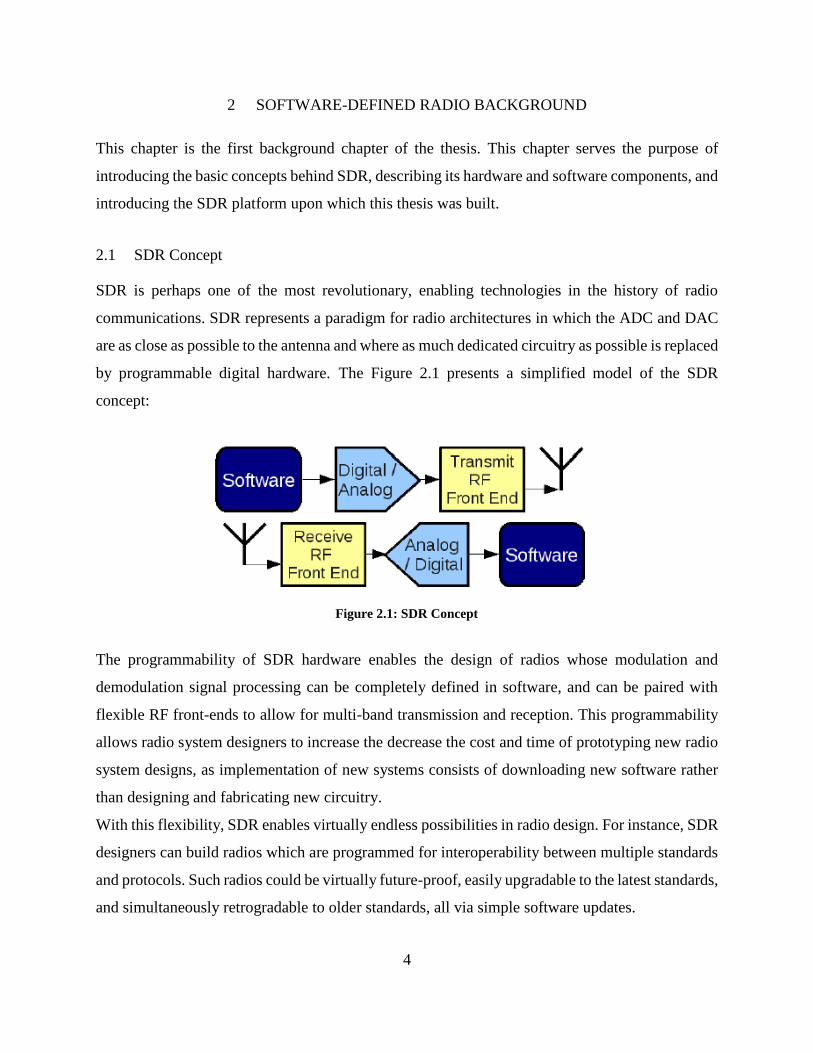
2.1 SDR Concept
SDR is perhaps one of the most revolutionary, enabling technologies in the history of radio
communications. SDR represents a paradigm for radio architectures in which the ADC and DAC
are as close as possible to the antenna and where as much dedicated circuitry as possible is replaced
by programmable digital hardware. The Figure 2.1 presents a simplified model of the SDR
concept:
The programmability of SDR hardware enables the design of radios whose modulation and
demodulation signal processing can be completely defined in software, and can be paired with
flexible RF front-ends to allow for multi-band transmission and reception. This programmability
allows radio system designers to increase the decrease the cost and time of prototyping new radio
system designs, as implementation of new systems consists of downloading new software rather
than designing and fabricating new circuitry.
With this flexibility, SDR enables virtually endless possibilities in radio design. For instance, SDR
designers can build radios which are programmed for interoperability between multiple standards
and protocols. Such radios could be virtually future-proof, easily upgradable to the latest standards,
and simultaneously retrogradable to older standards, all via simple software updates.
Figure 2.1: SDR Concept
5
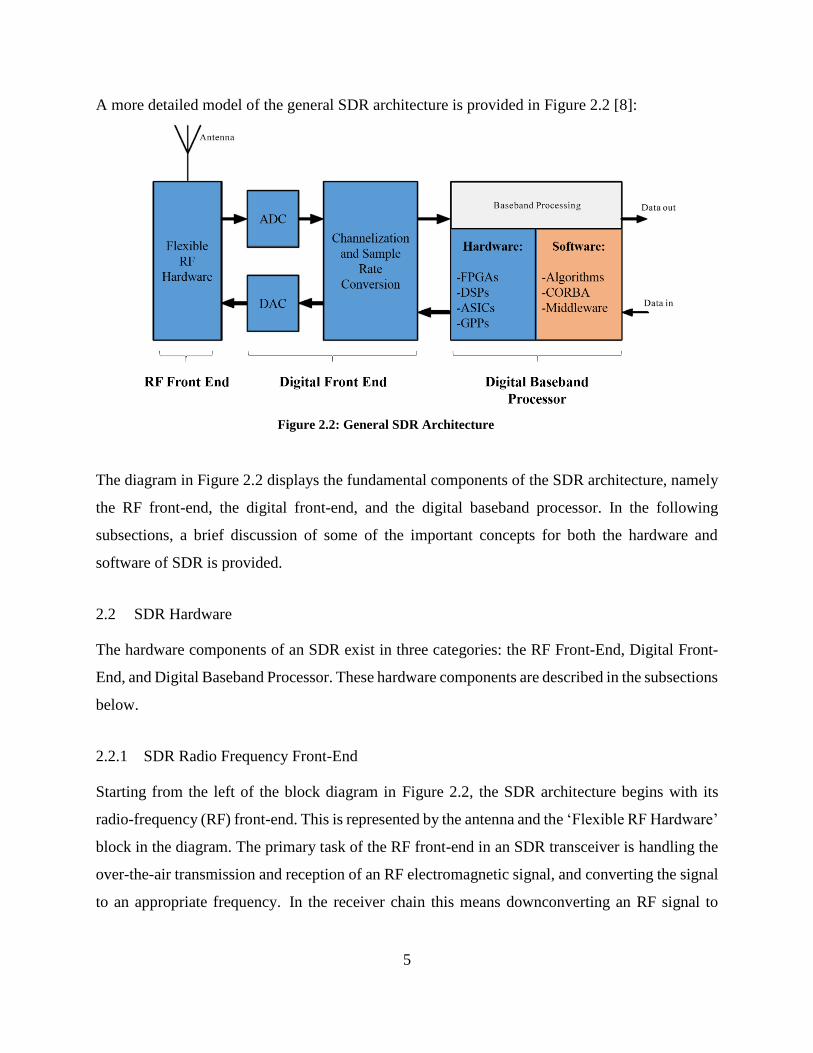
A more detailed model of the general SDR architecture is provided in Figure 2.2 [8]:
The diagram in Figure 2.2 displays the fundamental components of the SDR architecture, namely
the RF front-end, the digital front-end, and the digital baseband processor. In the following
subsections, a brief discussion of some of the important concepts for both the hardware and
software of SDR is provided.
2.2 SDR Hardware
The hardware components of an SDR exist in three categories: the RF Front-End, Digital Front-
End, and Digital Baseband Processor. These hardware components are described in the subsections
below.
2.2.1 SDR Radio Frequency Front-End
Starting from the left of the block diagram in Figure 2.2, the SDR architecture begins with its
radio-frequency (RF) front-end. This is represented by the antenna and the ‘Flexible RF Hardware’
block in the diagram. The primary task of the RF front-end in an SDR transceiver is handling the
over-the-air transmission and reception of an RF electromagnetic signal, and converting the signal
to an appropriate frequency. In the receiver chain this means downconverting an RF signal to
Figure 2.2: General SDR Architecture
6
baseband frequency, and in the transmitter chain this means upconverting a baseband analog signal
to the appropriate RF frequency for transmission.
The RF front-end module for both receiver and transmitter will be composed of a chain of analog
and digital circuits, including a number of filters, amplifiers, voltage-controlled oscillators (VCO),
and phase-locked loops (PLL). The RF front-end is largely composed of dedicated circuitry, but
many of these components are tunable and enable the reception and transmission of RF signals in
multiple bands and at variable power levels [8].
2.2.2 SDR Digital Front-End
Connected to the SDR RF front-end is its digital front-end (DFE). Figure 2.2 shows the digital
front-end module as being composed of ADC and DAC blocks and a channelization and sample
rate conversion block. The purpose of the DFE is to interface between the SDR RF front-end and
its digital baseband processor. In doing this, the DFE performs a couple major goals:
The first task of the DFE, in an SDR receiver, is to sample and digitize a downconverted baseband
analog signal received by the RF front-end. This task is performed by an ADC, and the output will
be a Nyquist-sampled, high sample-rate, digital signal representation of a broadband RF channel.
The second task of the DFE is to select a desired channel from the broadband signal,
channelization, and to reduce the high sample-rate of the signal to a minimum in order to avoid
excessive computation in the digital baseband demodulator, sample-rate conversion.
In an SDR transmitter chain these processes occur in reverse: a minimally-sampled baseband
signal is upsampled before being input to a DAC. The DAC produces the analog baseband signal
to be upconverted and transmitted by the RF front-end.
2.2.3 SDR Baseband Digital Processor
The heart of an SDR can probably be considered to be its digital baseband processor. This is a
programmable digital processor platform upon which real-time modulation and demodulation of
digital baseband signals are performed. Signal processing routines such as digital filtering,
encoding/decoding, interleaving/de-interleaving, and equalization are programmed in software
instructions which are executed by the baseband processor.
One of a number of programmable digital processor architectures can be employed in SDR. These
include digital signal processors (DSP), field-programmable gate arrays (FPGA), and general-
7
purpose processors (GPP). A choice of one of these digital processors typically requires a trade-
off between performance, computational efficiency, and programmability. The choice of platform
is an important decision, and based on the needs of the SDR designer. In this thesis, the
implemented SDR employs a GPP in the form of a personal computer CPU as the hardware
platform of the digital baseband processing unit.
2.3 SDR Software
The software component of an SDR describes the software instructions used to program the digital
baseband processor. These instructions program the processor to perform the signal processing
computations which modulate and demodulate an information-carrying, digital-baseband signal.
A variety of SDR software development frameworks exist, but the software development
environment chosen to implement the SDR of this thesis is called GNU Radio.
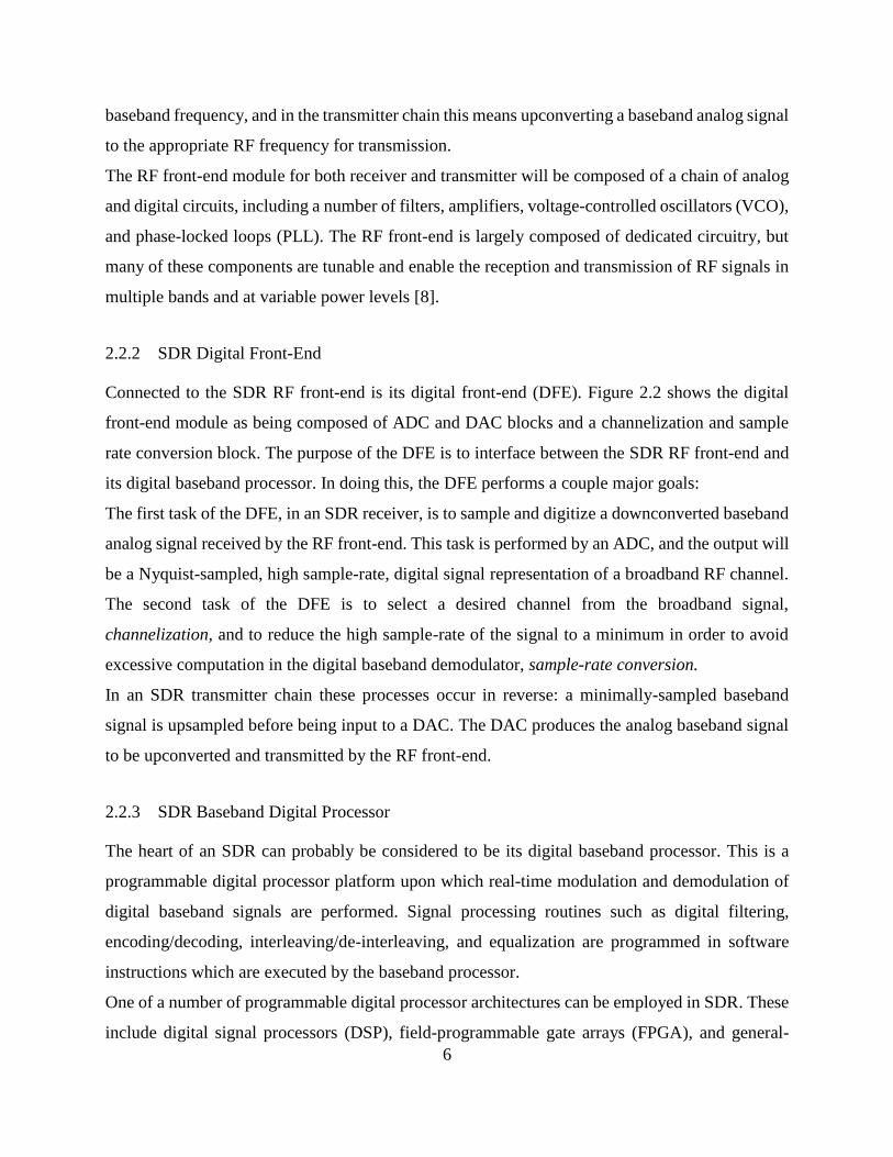
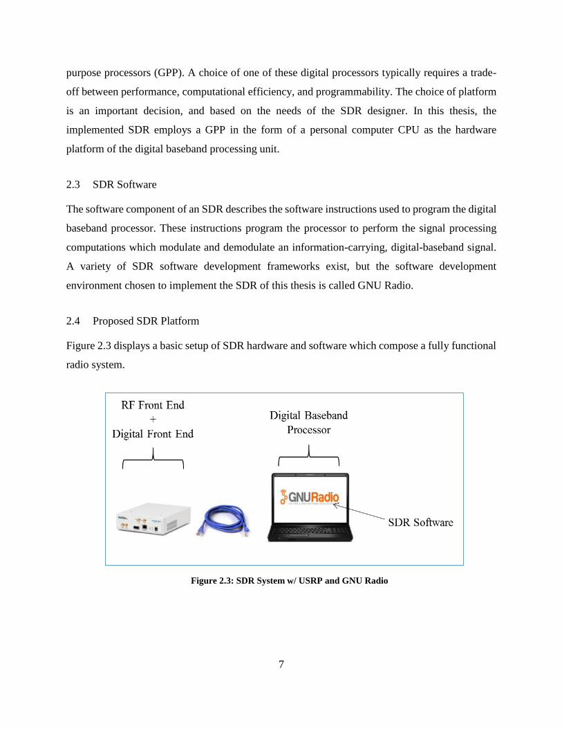
2.4 Proposed SDR Platform
Figure 2.3 displays a basic setup of SDR hardware and software which compose a fully functional
radio system.
Figure 2.3: SDR System w/ USRP and GNU Radio
8
In Figure 2.3, an Ettus Universal Software Radio Peripheral (USRP), which contains RF and digital
front end circuitry, is interfaced via gigabit Ethernet with a digital baseband processor in the form
of a personal computer running GNU Radio applications.
Chapter 6 details the implementation of the baseband modulation and demodulation of a constant
envelope OFDM waveform using the GNU Radio software. To begin an analysis of the waveform,
Chapter 3 provides background of the OFDM multicarrier modulation scheme.

9
3 ORTHOGONAL FREQUENCY-DIVISION MULTIPLEXING BACKGROUND
OFDM, Orthogonal Frequency-Division Multiplexing, is a modulation technique which has
revolutionized the wireless communications industry. OFDM is a multicarrier scheme, which
divides a wideband signal into multiple narrower bands of spectrum such that the aggregate signal
does not suffer the total impact of the fading in a wideband multipath channel. This lends OFDM
its inherent ability to enable high-speed communication on harsh wideband multipath channels
without the need for complex channel equalization. This virtue has made OFDM a favorite
modulation technique for 802.11 Wi-Fi protocols, and the 4G cellular standards, which must
support wideband data traffic over wireless channels.
This chapter presents the critical properties of OFDM. It begins with a cursory treatment of the
impairments caused by multipath channels and their representations in both the time and frequency
domain, and continues with an analytical description of OFDM and the properties which build its
immunity to multipath fading effects. The digital implementation of OFDM along with its various
benefits is then discussed before a consideration of its chief drawback- namely the PAPR problem.
3.1 Multipath Fading Phenomena
In a multipath channel, a transmitted signal will be reflected and scattered along multiple paths
which arrive at the receiver at different times and with different amplitudes. Figure 3.1 pictorially
represents the multipath scatterers of a signal in a wireless channel.
When the incident path, or the earliest-arriving signal, arrives at the receiver it is combined with
energy from multiple delayed reflections of itself. For this reason, the channel is said to spread the
Figure 3.1: Multipath Signal Propagation
10
signal in time. This results in a harmful, fluctuating distortion on the amplitude of the incident
signal - an effect called multipath fading.
While multipath fading can critically impair many communication systems, the properties of
OFDM signals allow them to endure multipath fading with considerable grace. To understand how
OFDM performs it is helpful to consider the frequency and time-domain properties of a multipath
channel, and then the frequency and time-domain properties of an OFDM signal.
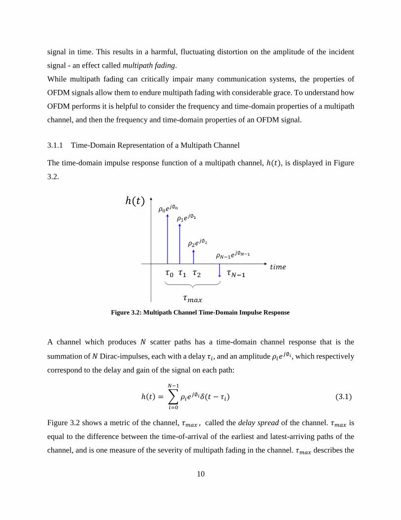
3.1.1 Time-Domain Representation of a Multipath Channel
The time-domain impulse response function of a multipath channel, ℎ(𝑡), is displayed in Figure
3.2.
A channel which produces 𝑁 scatter paths has a time-domain channel response that is the
summation of 𝑁 Dirac-impulses, each with a delay 𝜏𝑖, and an amplitude 𝜌𝑖𝑒𝑗∅𝑖, which respectively
correspond to the delay and gain of the signal on each path:
ℎ(𝑡) = ∑ 𝜌𝑖𝑒𝑗∅𝑖𝛿(𝑡 − 𝜏𝑖)
𝑁−1
𝑖=0
(3.1)
Figure 3.2 shows a metric of the channel, 𝜏𝑚𝑎𝑥 , called the delay spread of the channel. 𝜏𝑚𝑎𝑥 is
equal to the difference between the time-of-arrival of the earliest and latest-arriving paths of the
channel, and is one measure of the severity of multipath fading in the channel. 𝜏𝑚𝑎𝑥 describes the
Figure 3.2: Multipath Channel Time-Domain Impulse Response
11
duration over which signal’s energy will continue echoing, or spreading, in the channel after it has
been received on the incident path [17].
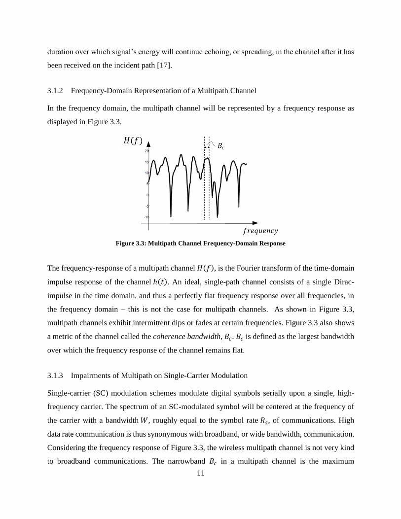
3.1.2 Frequency-Domain Representation of a Multipath Channel
In the frequency domain, the multipath channel will be represented by a frequency response as
displayed in Figure 3.3.
The frequency-response of a multipath channel 𝐻(𝑓), is the Fourier transform of the time-domain
impulse response of the channel ℎ(𝑡). An ideal, single-path channel consists of a single Dirac-
impulse in the time domain, and thus a perfectly flat frequency response over all frequencies, in
the frequency domain – this is not the case for multipath channels. As shown in Figure 3.3,
multipath channels exhibit intermittent dips or fades at certain frequencies. Figure 3.3 also shows
a metric of the channel called the coherence bandwidth, 𝐵𝑐. 𝐵𝑐 is defined as the largest bandwidth
over which the frequency response of the channel remains flat.
3.1.3 Impairments of Multipath on Single-Carrier Modulation
Single-carrier (SC) modulation schemes modulate digital symbols serially upon a single, high-
frequency carrier. The spectrum of an SC-modulated symbol will be centered at the frequency of
the carrier with a bandwidth 𝑊, roughly equal to the symbol rate 𝑅𝑠, of communications. High
data rate communication is thus synonymous with broadband, or wide bandwidth, communication.
Considering the frequency response of Figure 3.3, the wireless multipath channel is not very kind
to broadband communications. The narrowband 𝐵𝑐 in a multipath channel is the maximum
Figure 3.3: Multipath Channel Frequency-Domain Response
12
bandwidth that a signal can occupy in order to observe a flat-frequency response. This means that
the wideband symbols of high-speed SC modulation (𝑊 ≫ 𝐵𝑐) will be deeply, possibly
irreparably, distorted in a phenomena called frequency-selective fading.
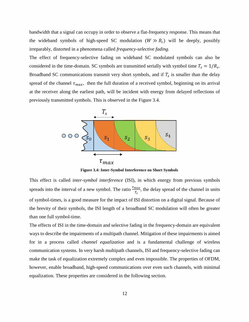
The effect of frequency-selective fading on wideband SC modulated symbols can also be
considered in the time-domain. SC symbols are transmitted serially with symbol time 𝑇𝑠 = 1/𝑅𝑠.
Broadband SC communications transmit very short symbols, and if 𝑇𝑠 is smaller than the delay
spread of the channel 𝜏𝑚𝑎𝑥, then the full duration of a received symbol, beginning on its arrival
at the receiver along the earliest path, will be incident with energy from delayed reflections of
previously transmitted symbols. This is observed in the Figure 3.4.
This effect is called inter-symbol interference (ISI), in which energy from previous symbols
spreads into the interval of a new symbol. The ratio 𝜏𝑚𝑎𝑥
𝑇𝑠, the delay spread of the channel in units
of symbol-times, is a good measure for the impact of ISI distortion on a digital signal. Because of
the brevity of their symbols, the ISI length of a broadband SC modulation will often be greater
than one full symbol-time.
The effects of ISI in the time-domain and selective fading in the frequency-domain are equivalent
ways to describe the impairments of a multipath channel. Mitigation of these impairments is aimed
for in a process called channel equalization and is a fundamental challenge of wireless
communication systems. In very harsh multipath channels, ISI and frequency-selective fading can
make the task of equalization extremely complex and even impossible. The properties of OFDM,
however, enable broadband, high-speed communications over even such channels, with minimal
equalization. These properties are considered in the following section.
Figure 3.4: Inter-Symbol Interference on Short Symbols
𝜏𝑚𝑎𝑥
13
Figure 3.5: Single Carrier Modulation Figure 3.6: Multi-Carrier Modulation
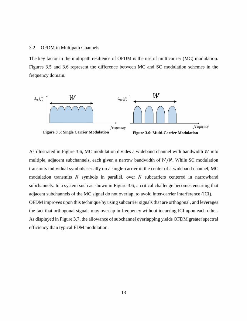
3.2 OFDM in Multipath Channels
The key factor in the multipath resilience of OFDM is the use of multicarrier (MC) modulation.
Figures 3.5 and 3.6 represent the difference between MC and SC modulation schemes in the
frequency domain.
As illustrated in Figure 3.6, MC modulation divides a wideband channel with bandwidth 𝑊 into
multiple, adjacent subchannels, each given a narrow bandwidth of 𝑊/𝑁. While SC modulation
transmits individual symbols serially on a single-carrier in the center of a wideband channel, MC
modulation transmits 𝑁 symbols in parallel, over 𝑁 subcarriers centered in narrowband
subchannels. In a system such as shown in Figure 3.6, a critical challenge becomes ensuring that
adjacent subchannels of the MC signal do not overlap, to avoid inter-carrier interference (ICI).
OFDM improves upon this technique by using subcarrier signals that are orthogonal, and leverages
the fact that orthogonal signals may overlap in frequency without incurring ICI upon each other.
As displayed in Figure 3.7, the allowance of subchannel overlapping yields OFDM greater spectral
efficiency than typical FDM modulation.
𝑊 𝑊

14
3.2.1 Frequency-Selective Fading Immunity of OFDM
OFDM subcarriers are packed tightly in frequency with a separation, ∆𝑓 = 𝑊/𝑁, where 𝑁 is
equal to the number of OFDM subcarriers. OFDM systems can be designed with 𝑁 large enough
such that ∆𝑓, which is also the effective bandwidth of subchannels, becomes less than 𝐵𝑐 of a
multipath channel. In this way, each of the narrowband OFDM subchannels will observe a
relatively flat channel-response. The figure 3.8 shows how OFDM divides a wideband multipath
channel with bandwidth 𝑊 into 𝑁, ∆𝑓 wide subchannels, the fading on each of which can be
equalized very simply with single-tap equalizers.
3.2.2 Inter-Symbol-Interference Immunity of OFDM
The narrowband subcarriers of OFDM require long symbol durations. To satisfy orthogonality it
is necessary that the symbol duration of each OFDM subcarrier be related to its frequency
separation by, 𝑇𝑠 = 1/∆𝑓. Because 1/∆𝑓 = 𝑁/𝑊 , this means that the duration of one aggregate
Figure 3.7: OFDM Modulation
𝑊
Figure 3.8: Subchannelization of Wideband Multipath Channel
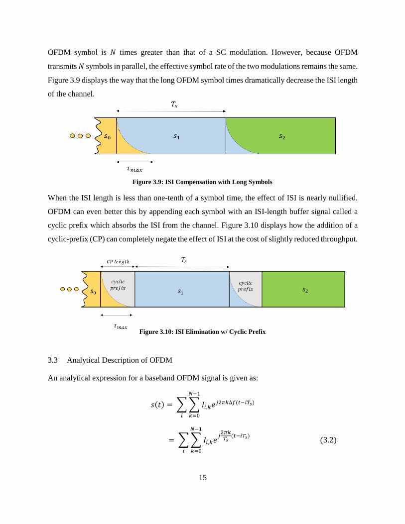
15
OFDM symbol is 𝑁 times greater than that of a SC modulation. However, because OFDM
transmits 𝑁 symbols in parallel, the effective symbol rate of the two modulations remains the same.
Figure 3.9 displays the way that the long OFDM symbol times dramatically decrease the ISI length
of the channel.
When the ISI length is less than one-tenth of a symbol time, the effect of ISI is nearly nullified.
OFDM can even better this by appending each symbol with an ISI-length buffer signal called a
cyclic prefix which absorbs the ISI from the channel. Figure 3.10 displays how the addition of a
cyclic-prefix (CP) can completely negate the effect of ISI at the cost of slightly reduced throughput.
3.3 Analytical Description of OFDM
An analytical expression for a baseband OFDM signal is given as:
𝑠(𝑡) = ∑ ∑ 𝐼𝑖,𝑘𝑒𝑗2𝜋𝑘∆𝑓(𝑡−𝑖𝑇𝑠)
𝑁−1
𝑘=0𝑖
= ∑ ∑ 𝐼𝑖,𝑘𝑒𝑗
2𝜋𝑘𝑇𝑠
(𝑡−𝑖𝑇𝑠)
𝑁−1
𝑘=0𝑖
(3.2)
Figure 3.10: ISI Elimination w/ Cyclic Prefix
Figure 3.9: ISI Compensation with Long Symbols

16
This expression shows that in the 𝑖th symbol interval, the OFDM signal will be composed of a
summation of 𝑁 subcarriers {𝑒𝑗2𝜋𝑘𝑡
𝑇𝑠 } 𝑘=0𝑁−1 , each modulated by a different symbol 𝐼𝑖,𝑘. The
subcarrier expression in (3.2) shows that the frequency of each complex sinusoid in the summation
is a multiple 𝑘 of the frequency separation ∆𝑓. This property ensures that all subcarriers in the set
are mutually orthogonal signals:
1
𝑇𝑠∫(𝑒𝑗2𝜋𝑓𝑘1𝑡) · (𝑒−𝑗2𝜋𝑓𝑘2𝑡)𝑑𝑡
𝑇𝑠
0
= 1
𝑇𝑠∫ 𝑒𝑗2𝜋(𝑓𝑘1−𝑓𝑘2
)𝑡𝑑𝑡
𝑇𝑠
0
(3.3)
= {0, 𝑘1 ≠ 𝑘2,
1, 𝑘1 = 𝑘2,
where, 𝑓𝑘𝑖= 𝑘𝑖∆𝑓 = 𝑘𝑖/𝑇𝑠
3.3.1 Digital Implementation of OFDM
One of the greatest luxuries of OFDM is its ability to be processed completely in the digital domain
with digital hardware, using the FFT algorithm. The discrete-time expression for a Nyquist-
sampled OFDM symbol, sampled at 𝑁 equally-spaced time instances is given by:
𝑠[𝑛] ≡ 𝑠(𝑡)| 𝑡=
𝑛𝑇𝑠𝑁
= ∑ 𝐼0,𝑘𝑒𝑗2𝜋𝑘𝑛
𝑁 , 𝑛 = 0, 1, … 𝑁 − 1
𝑁−1
𝑘=0
(3.4)
The set {𝐼0,𝑘}𝑘=0𝑁−1 is the set of symbols which modulates the 𝑁 subcarriers of the OFDM symbol
group. Equation (3.4) shows that the discrete-time OFDM baseband signal 𝑠[𝑛] is equivalent to
the inverse Discrete Fourier Transform (IDFT) of the symbol vector {𝐼0,𝑘}𝑘=0𝑁−1 , the elements of
which are the 𝑁 parallel symbols which modulate the 𝑁 OFDM subcarriers. Thus the synthesis
and modulation the 𝑁 orthogonal OFDM subcarriers is conveniently performed by an IDFT. The
IDFT is equivalently processed with greater computational efficiency by the inverse Fast-Fourier
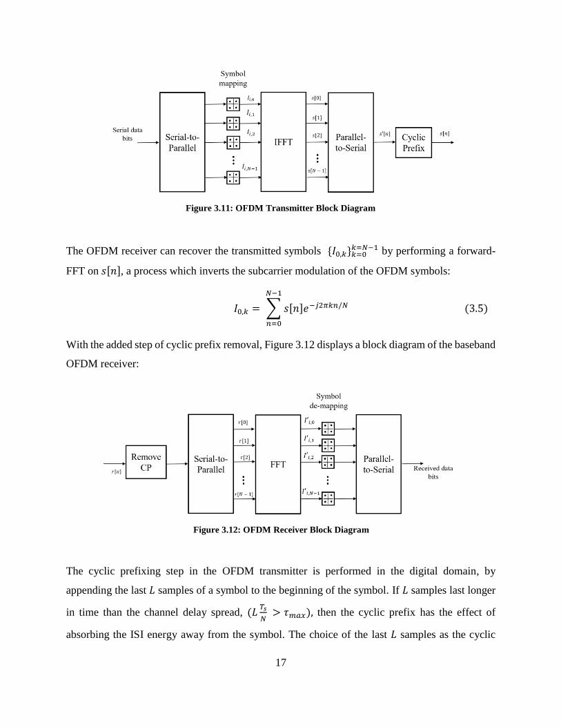
Transform (IFFT) algorithm. With the addition of the cyclic prefixing, Figure 3.11, displays a
block diagram of the baseband OFDM transmitter.
17
The OFDM receiver can recover the transmitted symbols {𝐼0,𝑘}𝑘=0𝑘=𝑁−1 by performing a forward-
FFT on 𝑠[𝑛], a process which inverts the subcarrier modulation of the OFDM symbols:
𝐼0,𝑘 = ∑ 𝑠[𝑛]𝑒−𝑗2𝜋𝑘𝑛/𝑁
𝑁−1
𝑛=0
(3.5)
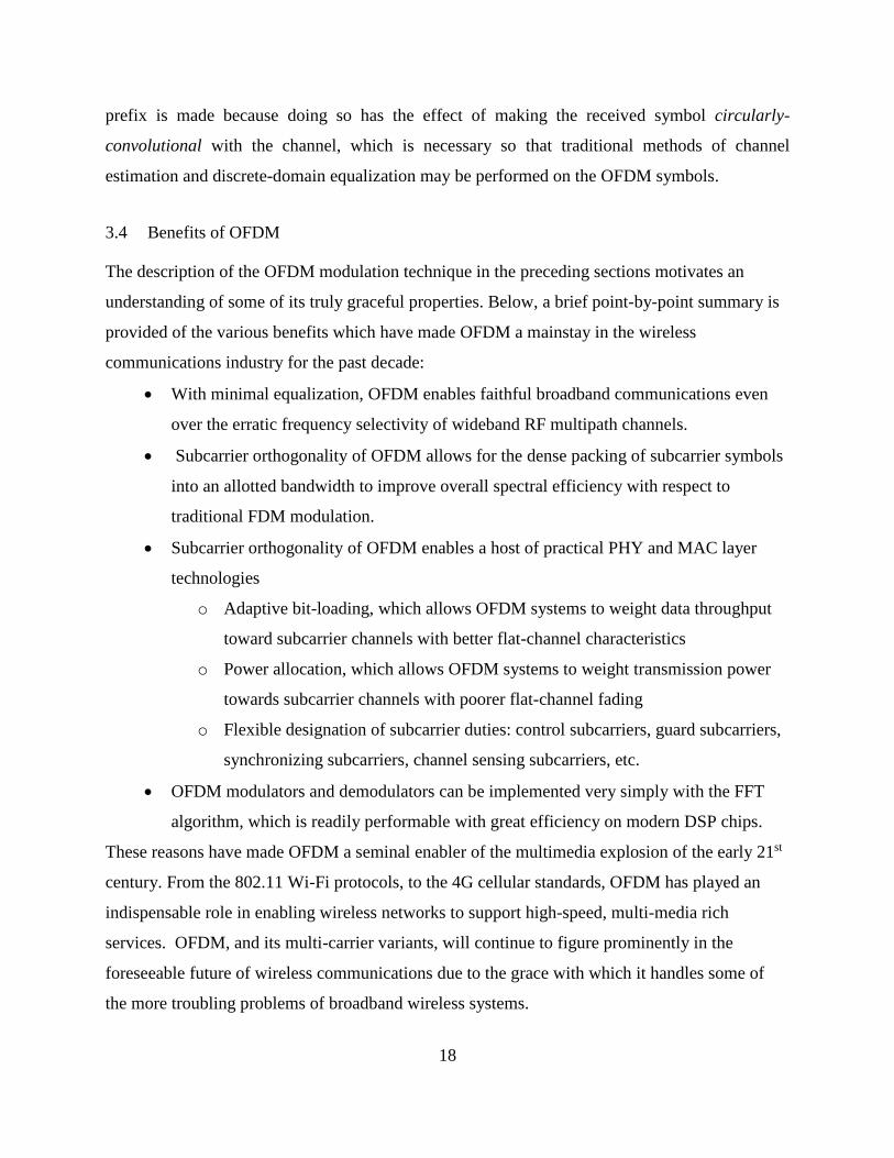
With the added step of cyclic prefix removal, Figure 3.12 displays a block diagram of the baseband
OFDM receiver:
The cyclic prefixing step in the OFDM transmitter is performed in the digital domain, by
appending the last 𝐿 samples of a symbol to the beginning of the symbol. If 𝐿 samples last longer
in time than the channel delay spread, (𝐿𝑇𝑠
𝑁 > 𝜏𝑚𝑎𝑥), then the cyclic prefix has the effect of
absorbing the ISI energy away from the symbol. The choice of the last 𝐿 samples as the cyclic
Figure 3.11: OFDM Transmitter Block Diagram
Figure 3.12: OFDM Receiver Block Diagram
18
prefix is made because doing so has the effect of making the received symbol circularly-
convolutional with the channel, which is necessary so that traditional methods of channel
estimation and discrete-domain equalization may be performed on the OFDM symbols.
3.4 Benefits of OFDM
The description of the OFDM modulation technique in the preceding sections motivates an
understanding of some of its truly graceful properties. Below, a brief point-by-point summary is
provided of the various benefits which have made OFDM a mainstay in the wireless
communications industry for the past decade:
With minimal equalization, OFDM enables faithful broadband communications even
over the erratic frequency selectivity of wideband RF multipath channels.
Subcarrier orthogonality of OFDM allows for the dense packing of subcarrier symbols
into an allotted bandwidth to improve overall spectral efficiency with respect to
traditional FDM modulation.
Subcarrier orthogonality of OFDM enables a host of practical PHY and MAC layer
technologies
o Adaptive bit-loading, which allows OFDM systems to weight data throughput
toward subcarrier channels with better flat-channel characteristics
o Power allocation, which allows OFDM systems to weight transmission power
towards subcarrier channels with poorer flat-channel fading
o Flexible designation of subcarrier duties: control subcarriers, guard subcarriers,
synchronizing subcarriers, channel sensing subcarriers, etc.
OFDM modulators and demodulators can be implemented very simply with the FFT
algorithm, which is readily performable with great efficiency on modern DSP chips.
These reasons have made OFDM a seminal enabler of the multimedia explosion of the early 21st
century. From the 802.11 Wi-Fi protocols, to the 4G cellular standards, OFDM has played an
indispensable role in enabling wireless networks to support high-speed, multi-media rich
services. OFDM, and its multi-carrier variants, will continue to figure prominently in the
foreseeable future of wireless communications due to the grace with which it handles some of
the more troubling problems of broadband wireless systems.

19
As is true of any technology, OFDM is not without critical faults and design challenges. The
benefits of OFDM must be reconciled with its inherently high peak-to-average power ratio
(PAPR) – a dilemma often termed the PAPR problem. The purpose of the following chapter of
this thesis is to motivate an understanding of OFDM’s PAPR problem as well as its critical
implications for the power efficiency of OFDM and its multicarrier variants, and its broader
implications concerning the sustainability of an increasingly OFDM and multicarrier enabled
generation of multimedia wireless communications.
20
4 THE PROBLEM OF PEAK-TO-AVERAGE POWER RATIO IN OFDM
For the harmony OFDM orchestrates in enabling broadband multipath communication, OFDM
conducts a seemingly perfect storm for the job of power amplification. The key culprit in this
matter is the high peak-to-power-ratio (PAPR). The PAPR of a signal is defined as the ratio of a
peak instantaneous power to the average power of a signal:
𝑃𝐴𝑃𝑅{𝑥(𝑡)} =𝑝𝑒𝑎𝑘 𝑠𝑖𝑔𝑛𝑎𝑙 𝑝𝑜𝑤𝑒𝑟
𝑎𝑣𝑒𝑟𝑎𝑔𝑒 𝑠𝑖𝑔𝑛𝑎𝑙 𝑝𝑜𝑤𝑒𝑟=
max {𝑥2(𝑡)}
𝐸{𝑥2(𝑡)}
In Section 4.1 a qualitative and quantitative discussion of the OFDM PAPR problem is provided,
in Section 4.2 a discussion of power amplification of OFDM is provided to detail the impact of
high PAPR amplification on power efficiency, and Section 4.3 closes with a discussion of the
implications of the power inefficiency of OFDM.
4.1 PAPR Statistics of OFDM
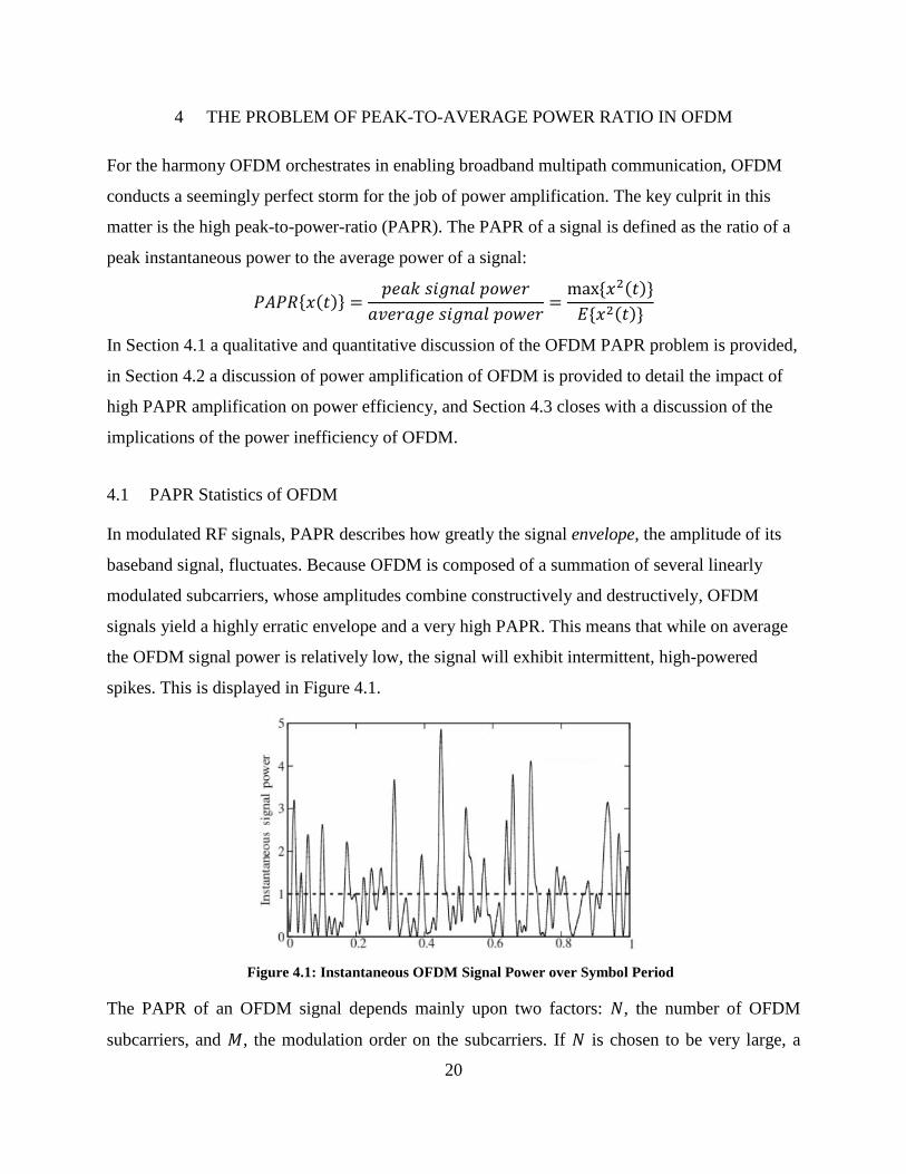
In modulated RF signals, PAPR describes how greatly the signal envelope, the amplitude of its
baseband signal, fluctuates. Because OFDM is composed of a summation of several linearly
modulated subcarriers, whose amplitudes combine constructively and destructively, OFDM
signals yield a highly erratic envelope and a very high PAPR. This means that while on average
the OFDM signal power is relatively low, the signal will exhibit intermittent, high-powered
spikes. This is displayed in Figure 4.1.
The PAPR of an OFDM signal depends mainly upon two factors: 𝑁, the number of OFDM
subcarriers, and 𝑀, the modulation order on the subcarriers. If 𝑁 is chosen to be very large, a
Figure 4.1: Instantaneous OFDM Signal Power over Symbol Period
21
design choice which increases spectral efficiency, the OFDM signal envelope will exhibit large
spikes whenever a majority of the subcarrier symbol amplitudes combine constructively.
If subcarriers are modulated on a constant envelope, such as via phase-shift keying (PSK), the
OFDM signal reaches its absolute peaks in the event that all 𝑁 symbols align in phase. If the
subcarriers are modulated with a non-constant envelope, such as with the highly spectrally-
efficient M-ary QAM modulation, the OFDM peaks are magnified yet further and reach absolute
crests when all symbols align in-phase, at their highest order amplitudes. In summary, the more
spectrally efficient the modulation is, the higher the PAPR will be. Table 4-1 provides values of
PAPR for various OFDM modulation parameters [7]:
Table 4-1: PAPR comparison for different OFDM modulation parameters
𝑄𝑃𝑆𝐾 16𝑄𝐴𝑀 64𝑄𝐴𝑀 256𝑄𝐴𝑀
𝑁 = 64 18 dB 20.4 dB 21.4 dB 22 dB
𝑁 = 128 21 dB 23.6 dB 24.6 dB 25.2 dB
𝑁 = 256 24 dB 26.5 dB 27.6 dB 28.1 dB
𝑁 = 512 27 dB 29.6 dB 30.7 dB 31.2 dB
𝑁 = 1024 30 dB 32.6 dB 33.7 dB 34.2 dB
The PAPR values in Table 4-1 tell a worst-case scenario for these OFDM signals, as they give a
ratio of the absolute peak power to the average power. The event of absolute peaks occurring
will be very rare if transmitted symbols can be modeled as independent and identically
distributed (i.i.d) random variables. Hence more relaxed measures of signal dynamic range are
often used such as the complementary cumulative distribution function (CCDF) of PAPR.
Without loss of generality, however, PAPR is used to motivate the forthcoming discussion, and
the next section of the chapter describes the impact of the OFDM’s high PAPR on the efficiency
of its power amplification.
4.2 Power Amplification of High-PAPR OFDM
Power amplification is a necessary stage in all wireless communications, as signals must be
given enough power to carry their message over a required distance with a required fidelity. The
greatest significance of the PAPR of a modulated signal is that the PAPR significantly affects the
ability of the signal to be processed by non-linear components of the radio circuitry. In this

22
section the power amplifier (PA) is considered as one such non-linear element of critical
importance, and the impact of high PAPR signal input on the power efficiency performance of a
PA is considered. To begin a brief overview of the basic concepts of power amplification is in
order.
4.2.1 Power Amplifier Basics
A PA can be generally characterized by the following parameters [15][20],
Peak Output Power, 𝑃𝑜𝑢𝑡𝑚𝑎𝑥
DC Power Supply, 𝑃𝐷𝐶
Drain Efficiency, 𝜂
Linearity
Gain
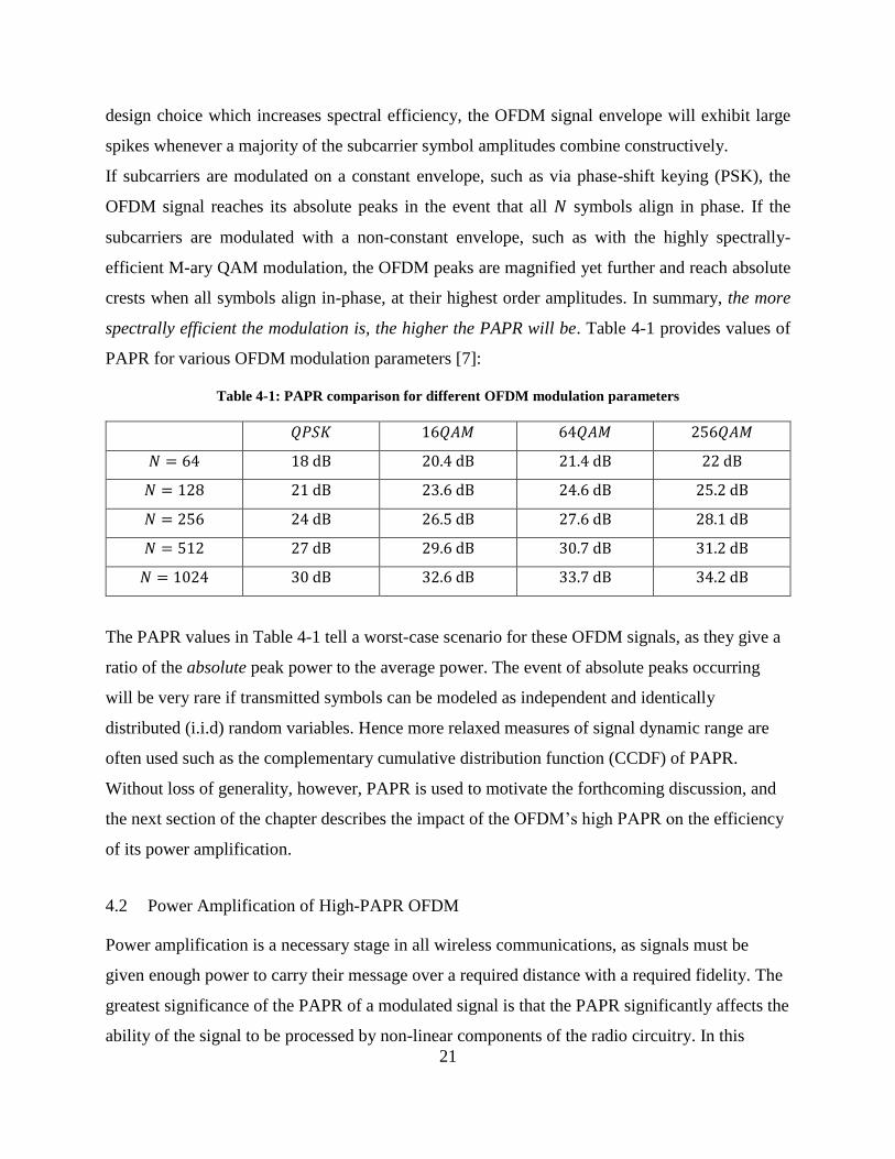
An ideal PA amplifies the input signal linearly by multiplying its amplitude with a fixed gain,
but such a PA does not exist. A real PA is a nonlinear device with only limited regions of
approximate linearity. The graph in Figure 4.2 shows the nonlinear amplitude-to-amplitude curve
(AM-AM) of a PA. This curve displays the input signal power against the output signal power
and describes many of the most important PA properties.
23
This provides a few critical figures of merit to discuss:
4.2.1.1 PA Operation Regions
The AM-AM curve in Figure 4.2 shows that a PA has a linear operation region in which the power
of the output signal is approximately equal to the power of the input signal multiplied by the
amplifier gain. The input signal can only be linearly amplified when its power is within a range
called the linear dynamic range. The upper limit of this range is often characterized by the 1-dB
compression point, a point where the gain applied to the input power becomes 1 dB less than the
nominal linear gain of the amplifier.
As the input signal power exceeds the linear dynamic range, the amplifier eventually reaches its
saturation region, where its peak output power is reached, and no further amplification can be
achieved.
4.2.1.2 PA Efficiency
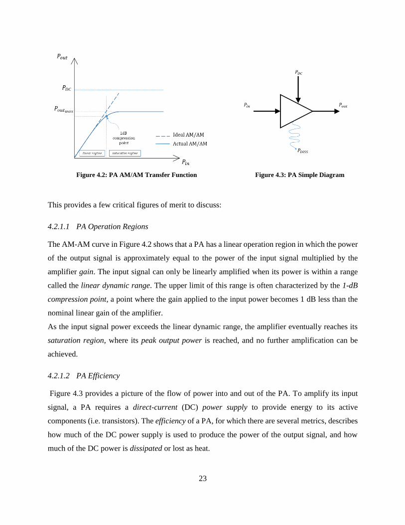
Figure 4.3 provides a picture of the flow of power into and out of the PA. To amplify its input
signal, a PA requires a direct-current (DC) power supply to provide energy to its active
components (i.e. transistors). The efficiency of a PA, for which there are several metrics, describes
how much of the DC power supply is used to produce the power of the output signal, and how
much of the DC power is dissipated or lost as heat.
Figure 4.2: PA AM/AM Transfer Function Figure 4.3: PA Simple Diagram
24
Figure 4.4: Effect of Operation Region on Drain Efficiency
One common efficiency measure is called the drain efficiency, 𝜂𝑑𝑟𝑎𝑖𝑛:
𝜂𝑑𝑟𝑎𝑖𝑛 =𝑃𝑜𝑢𝑡
𝑃𝐷𝐶 % (4.2)
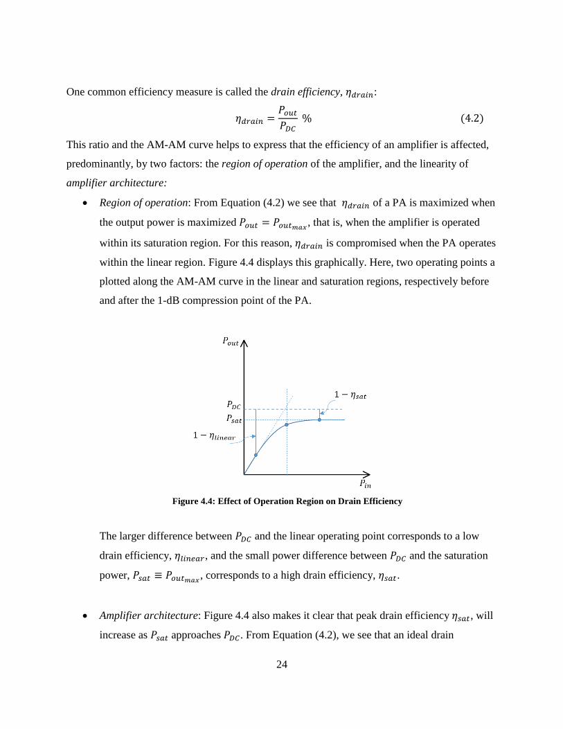
This ratio and the AM-AM curve helps to express that the efficiency of an amplifier is affected,
predominantly, by two factors: the region of operation of the amplifier, and the linearity of
amplifier architecture:
Region of operation: From Equation (4.2) we see that 𝜂𝑑𝑟𝑎𝑖𝑛 of a PA is maximized when
the output power is maximized 𝑃𝑜𝑢𝑡 = 𝑃𝑜𝑢𝑡𝑚𝑎𝑥, that is, when the amplifier is operated
within its saturation region. For this reason, 𝜂𝑑𝑟𝑎𝑖𝑛 is compromised when the PA operates
within the linear region. Figure 4.4 displays this graphically. Here, two operating points a
plotted along the AM-AM curve in the linear and saturation regions, respectively before
and after the 1-dB compression point of the PA.
The larger difference between 𝑃𝐷𝐶 and the linear operating point corresponds to a low
drain efficiency, 𝜂𝑙𝑖𝑛𝑒𝑎𝑟, and the small power difference between 𝑃𝐷𝐶 and the saturation
power, 𝑃𝑠𝑎𝑡 ≡ 𝑃𝑜𝑢𝑡𝑚𝑎𝑥, corresponds to a high drain efficiency, 𝜂𝑠𝑎𝑡.
Amplifier architecture: Figure 4.4 also makes it clear that peak drain efficiency 𝜂𝑠𝑎𝑡, will
increase as 𝑃𝑠𝑎𝑡 approaches 𝑃𝐷𝐶. From Equation (4.2), we see that an ideal drain
25
efficiency of 100% is achieved when operating a PA whose 𝑃𝐷𝐶 = 𝑃𝑠𝑎𝑡, in its saturation
region, 𝑃𝑜𝑢𝑡 = 𝑃𝑠𝑎𝑡.
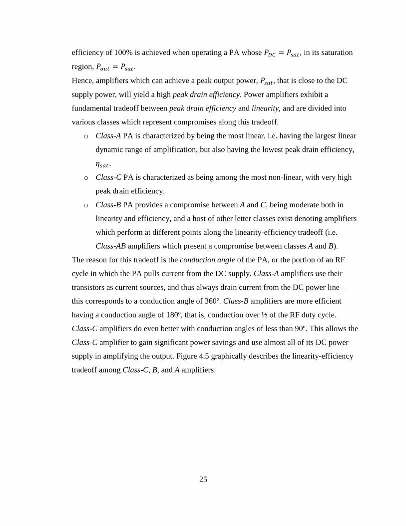
Hence, amplifiers which can achieve a peak output power, 𝑃𝑠𝑎𝑡 , that is close to the DC
supply power, will yield a high peak drain efficiency. Power amplifiers exhibit a
fundamental tradeoff between peak drain efficiency and linearity, and are divided into
various classes which represent compromises along this tradeoff.
o Class-A PA is characterized by being the most linear, i.e. having the largest linear
dynamic range of amplification, but also having the lowest peak drain efficiency,
𝜂𝑠𝑎𝑡.
o Class-C PA is characterized as being among the most non-linear, with very high
peak drain efficiency.
o Class-B PA provides a compromise between A and C, being moderate both in
linearity and efficiency, and a host of other letter classes exist denoting amplifiers
which perform at different points along the linearity-efficiency tradeoff (i.e.
Class-AB amplifiers which present a compromise between classes A and B).
The reason for this tradeoff is the conduction angle of the PA, or the portion of an RF
cycle in which the PA pulls current from the DC supply. Class-A amplifiers use their
transistors as current sources, and thus always drain current from the DC power line –
this corresponds to a conduction angle of 360º. Class-B amplifiers are more efficient
having a conduction angle of 180º, that is, conduction over ½ of the RF duty cycle.
Class-C amplifiers do even better with conduction angles of less than 90º. This allows the
Class-C amplifier to gain significant power savings and use almost all of its DC power
supply in amplifying the output. Figure 4.5 graphically describes the linearity-efficiency
tradeoff among Class-C, B, and A amplifiers:
26
Figure 4.2: Linearity-Efficiency Tradeoff among
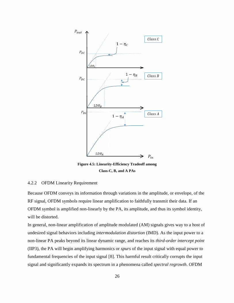
4.2.2 OFDM Linearity Requirement
Because OFDM conveys its information through variations in the amplitude, or envelope, of the
RF signal, OFDM symbols require linear amplification to faithfully transmit their data. If an
OFDM symbol is amplified non-linearly by the PA, its amplitude, and thus its symbol identity,
will be distorted.
In general, non-linear amplification of amplitude modulated (AM) signals gives way to a host of
undesired signal behaviors including intermodulation distortion (IMD). As the input power to a
non-linear PA peaks beyond its linear dynamic range, and reaches its third-order intercept point
(IIP3), the PA will begin amplifying harmonics or spurs of the input signal with equal power to
fundamental frequencies of the input signal [8]. This harmful result critically corrupts the input
signal and significantly expands its spectrum in a phenomena called spectral regrowth. OFDM
Figure 4.5: Linearity-Efficiency Tradeoff among
Class-C, B, and A PAs
27
then faces a critical dilemma. The high PAPR of OFDM demands high PA linearity to avoid
suffering these undesirable effects, and this demand for linearity results in a demand for PA
power inefficiency. The tradeoff between linearity and inefficiency in amplifying OFDM signals
is described in the following subsection.
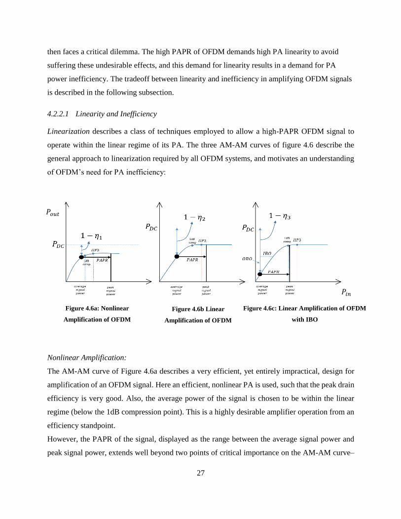
4.2.2.1 Linearity and Inefficiency
Linearization describes a class of techniques employed to allow a high-PAPR OFDM signal to
operate within the linear regime of its PA. The three AM-AM curves of figure 4.6 describe the
general approach to linearization required by all OFDM systems, and motivates an understanding
of OFDM’s need for PA inefficiency:
Nonlinear Amplification:
The AM-AM curve of Figure 4.6a describes a very efficient, yet entirely impractical, design for
amplification of an OFDM signal. Here an efficient, nonlinear PA is used, such that the peak drain
efficiency is very good. Also, the average power of the signal is chosen to be within the linear
regime (below the 1dB compression point). This is a highly desirable amplifier operation from an
efficiency standpoint.
However, the PAPR of the signal, displayed as the range between the average signal power and
peak signal power, extends well beyond two points of critical importance on the AM-AM curve–
Figure 4.6a: Nonlinear
Amplification of OFDM
Figure 4.6b Linear
Amplification of OFDM
Figure 4.6c: Linear Amplification of OFDM
with IBO
𝑃𝑜𝑢𝑡
𝑃𝑖𝑛

28
the 1dB compression point (which governs linear PA operation) and the IIP3 point (which governs
spurious free PA operation). Thus, this signal will be irreparably distorted, and will undergo
unacceptable spectral regrowth.
Linear Amplification w/o Power Backoff:
The AM-AM curve of Figure 4.6b does slightly better to remedy non-linear PA effects. Operating
at the same average power point, the transmitter now employs a PA with greater linearity. A look
at the signal PAPR shows that now about half of the PAPR range of the signal will fall within the
linear region of the amplifier. While better than the transmitter design in Figure 4.6a, this bodes
poorly for the fidelity of the amplitude-modulated symbols. The figure also shows that, in
comparison to the amplification in Figure 4.6a, much less of the signal PAPR range will exceed
the IIP3 point thus IIP3 distortion affects occur with lower probability.
Linear Amplification with Power Backoff:
The AM-AM curve in Figure 4.6c describes how the issues of Figures 4.6a and 4.6b are remedied
in typical OFDM transmitter architectures. The average power of the OFDM signal will be
‘backed-off’, or attenuated, before amplification to better contain the PAPR of the signal within
the linear and spurious free ranges. The level of attenuation is called input-power backoff (IBO)
and has a corresponding output-power backoff (OBO) as illustrated in Figure 4.6c. Now, a look at
the PAPR of the signal shows that the signal will no longer operate within the IIP3 range of the
PA, avoiding the harmful effects of intermodulation distortion and spectral regrowth, and will be
amplified linearly, i.e. within the 1dB compression point, over the close to the full range of the
input signal.
Figure 4.6c describes the general linearization approach required for power amplification of
OFDM signals. While it does well to achieve desired linearity, we see just how badly the average
drain efficiency of the PA, denoted by 𝜂3, suffers. Nearly all of the power provided by the PA DC
supply is wasted and dissipated as heat as only a small fraction is actually used to amplify the
signal. Without the use of added linearization technologies, OFDM will require drain efficiency
of less than 20% [6]!
29
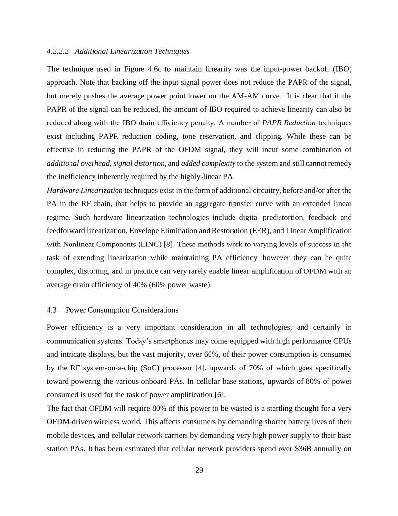
4.2.2.2 Additional Linearization Techniques
The technique used in Figure 4.6c to maintain linearity was the input-power backoff (IBO)
approach. Note that backing off the input signal power does not reduce the PAPR of the signal,
but merely pushes the average power point lower on the AM-AM curve. It is clear that if the
PAPR of the signal can be reduced, the amount of IBO required to achieve linearity can also be
reduced along with the IBO drain efficiency penalty. A number of PAPR Reduction techniques
exist including PAPR reduction coding, tone reservation, and clipping. While these can be
effective in reducing the PAPR of the OFDM signal, they will incur some combination of
additional overhead, signal distortion, and added complexity to the system and still cannot remedy
the inefficiency inherently required by the highly-linear PA.
Hardware Linearization techniques exist in the form of additional circuitry, before and/or after the
PA in the RF chain, that helps to provide an aggregate transfer curve with an extended linear
regime. Such hardware linearization technologies include digital predistortion, feedback and
feedforward linearization, Envelope Elimination and Restoration (EER), and Linear Amplification
with Nonlinear Components (LINC) [8]. These methods work to varying levels of success in the
task of extending linearization while maintaining PA efficiency, however they can be quite
complex, distorting, and in practice can very rarely enable linear amplification of OFDM with an
average drain efficiency of 40% (60% power waste).
4.3 Power Consumption Considerations
Power efficiency is a very important consideration in all technologies, and certainly in
communication systems. Today’s smartphones may come equipped with high performance CPUs
and intricate displays, but the vast majority, over 60%, of their power consumption is consumed
by the RF system-on-a-chip (SoC) processor [4], upwards of 70% of which goes specifically
toward powering the various onboard PAs. In cellular base stations, upwards of 80% of power
consumed is used for the task of power amplification [6].
The fact that OFDM will require 80% of this power to be wasted is a startling thought for a very
OFDM-driven wireless world. This affects consumers by demanding shorter battery lives of their
mobile devices, and cellular network carriers by demanding very high power supply to their base
station PAs. It has been estimated that cellular network providers spend over $36B annually on

30
powering their base stations [10]. Moreover, the communications industry is responsible for
roughly 10% of the global energy consumption and carbon footprint, and the environmental impact
of the wastefulness of OFDM PAs . As we continue to envision a world with greater wireless
connectivity, capacity, and throughput, it behooves us to consider optimally power-efficient
approaches to address the OFDM PAPR problem.
31
5 CONSTANT-ENVELOPE OFDM
The previous chapters have covered OFDM, considering the merits which have made it such an
important technology and also the PAPR problem which makes OFDM systems suffer large power
wastage. The OFDM PAPR problem can be summarized by the following: The inherently large
PAPR of OFDM demands highly linear power amplification, and by rule-of-thumb highly linear
power amplification is equivalent to highly inefficient power amplification. PAPR-reduction
techniques seek to reduce the power backoff required by OFDM before amplification, and
hardware linearization techniques seek to extend the linear operation regime of the power
amplifier, but to totally cure its power inefficiency woes, OFDM needs to be cured of the need for
highly linear amplification and RF processing. This is the motivation for the constant envelope
OFDM (CE-OFDM) waveform.
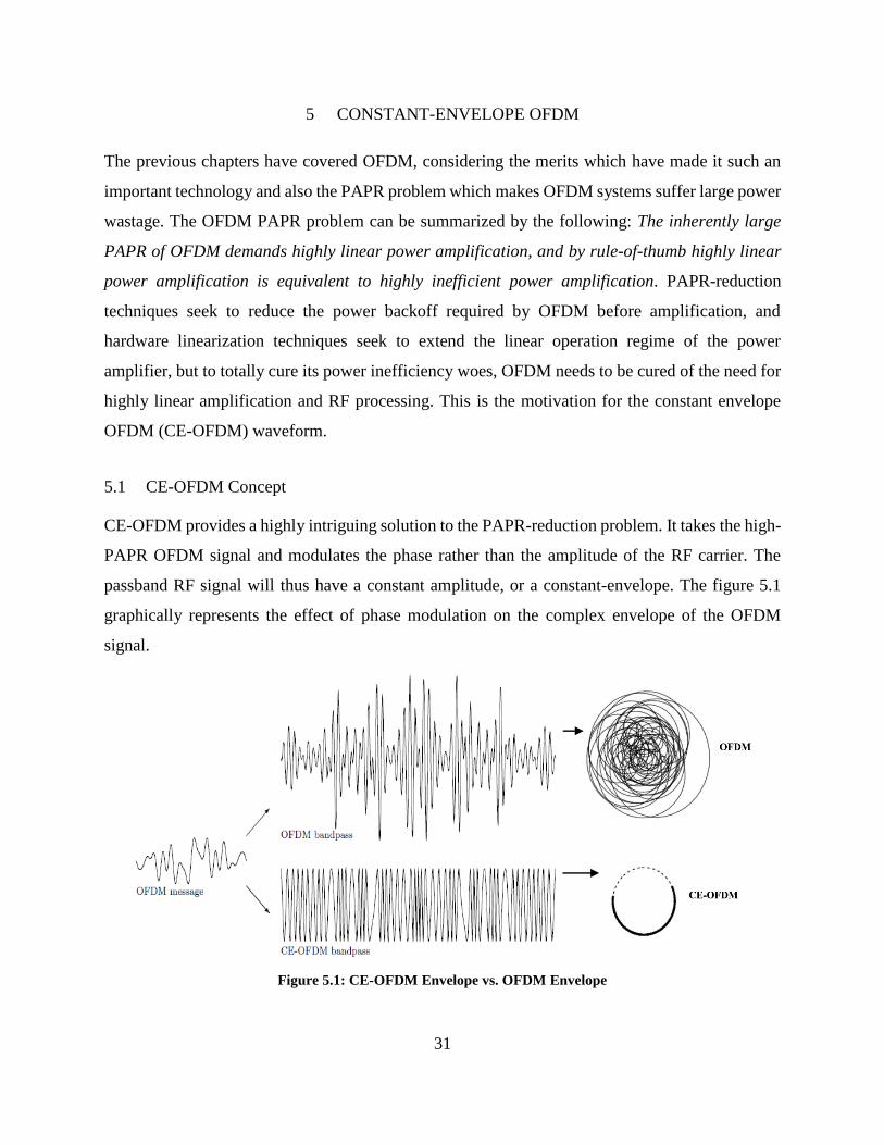
5.1 CE-OFDM Concept
CE-OFDM provides a highly intriguing solution to the PAPR-reduction problem. It takes the high-
PAPR OFDM signal and modulates the phase rather than the amplitude of the RF carrier. The
passband RF signal will thus have a constant amplitude, or a constant-envelope. The figure 5.1
graphically represents the effect of phase modulation on the complex envelope of the OFDM
signal.
Figure 5.1: CE-OFDM Envelope vs. OFDM Envelope
32
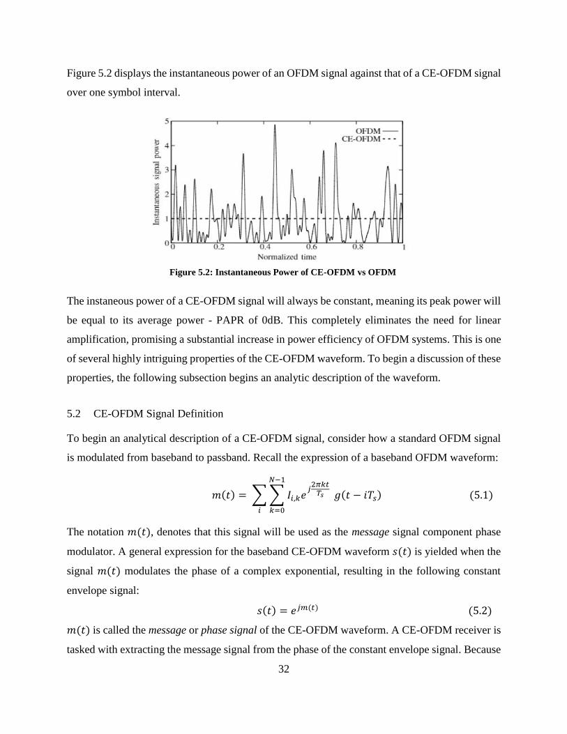
Figure 5.2 displays the instantaneous power of an OFDM signal against that of a CE-OFDM signal
over one symbol interval.
The instaneous power of a CE-OFDM signal will always be constant, meaning its peak power will
be equal to its average power - PAPR of 0dB. This completely eliminates the need for linear
amplification, promising a substantial increase in power efficiency of OFDM systems. This is one
of several highly intriguing properties of the CE-OFDM waveform. To begin a discussion of these
properties, the following subsection begins an analytic description of the waveform.
5.2 CE-OFDM Signal Definition
To begin an analytical description of a CE-OFDM signal, consider how a standard OFDM signal
is modulated from baseband to passband. Recall the expression of a baseband OFDM waveform:
𝑚(𝑡) = ∑ ∑ 𝐼𝑖,𝑘𝑒𝑗
2𝜋𝑘𝑡𝑇𝑠
𝑁−1
𝑘=0
𝑔(𝑡 − 𝑖𝑇𝑠)
𝑖
(5.1)
The notation 𝑚(𝑡), denotes that this signal will be used as the message signal component phase
modulator. A general expression for the baseband CE-OFDM waveform 𝑠(𝑡) is yielded when the
signal 𝑚(𝑡) modulates the phase of a complex exponential, resulting in the following constant
envelope signal:
𝑠(𝑡) = 𝑒𝑗𝑚(𝑡) (5.2)
𝑚(𝑡) is called the message or phase signal of the CE-OFDM waveform. A CE-OFDM receiver is
tasked with extracting the message signal from the phase of the constant envelope signal. Because
Figure 5.2: Instantaneous Power of CE-OFDM vs OFDM
33
the argument of a complex phasor must be a real, 𝑚(𝑡) in expression (5.2) must be a purely real
signal. This requires that symbol set, {𝐼𝑖,𝑘}, in 𝑚(𝑡) must also be purely real; that is, the message
signal of CE-OFDM can support only real-valued data symbols - those on a 1-dimensional
constellation. The implications of the latter are further considered in the performance analysis
section.
After passband modulation, the general CE-OFDM passband expression of (5.1) results:
𝑦(𝑡) = 𝑅𝑒{𝑠(𝑡) · 𝑒𝑗𝜔𝑐𝑡}
= 𝑅𝑒{𝑒𝑗(𝜔𝑐𝑡+𝑚(𝑡))}
= cos(𝜔𝑐𝑡 + 𝑚(𝑡)) (5.3)
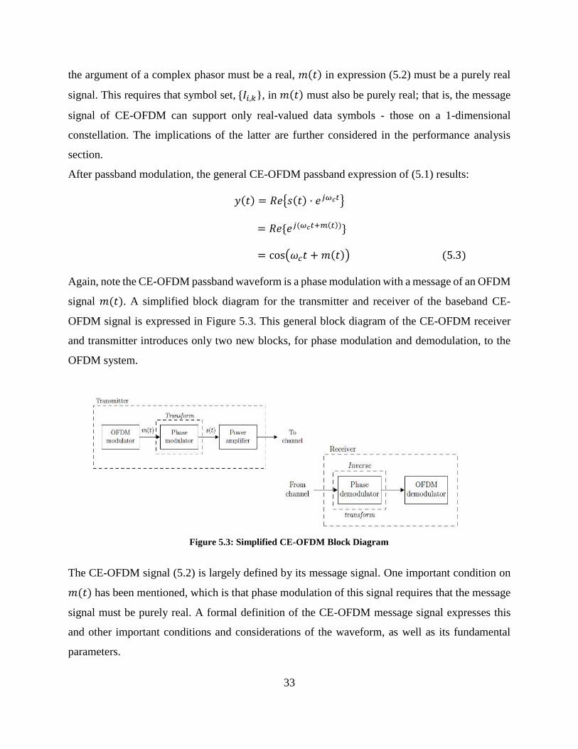
Again, note the CE-OFDM passband waveform is a phase modulation with a message of an OFDM
signal 𝑚(𝑡). A simplified block diagram for the transmitter and receiver of the baseband CE-
OFDM signal is expressed in Figure 5.3. This general block diagram of the CE-OFDM receiver
and transmitter introduces only two new blocks, for phase modulation and demodulation, to the
OFDM system.
The CE-OFDM signal (5.2) is largely defined by its message signal. One important condition on
𝑚(𝑡) has been mentioned, which is that phase modulation of this signal requires that the message
signal must be purely real. A formal definition of the CE-OFDM message signal expresses this
and other important conditions and considerations of the waveform, as well as its fundamental
parameters.
Figure 5.3: Simplified CE-OFDM Block Diagram
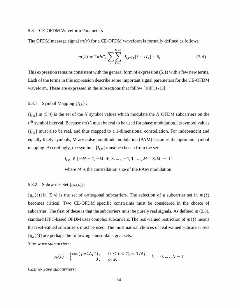
34
5.3 CE-OFDM Waveform Parameters
The OFDM message signal 𝑚(𝑡) for a CE-OFDM waveform is formally defined as follows:
𝑚(𝑡) = 2𝜋ℎ𝐶𝑛 ∑ ∑ 𝐼𝑖,𝑘𝑞𝑘[𝑡 − 𝑖𝑇𝑠] + 𝜃𝑖
𝑁−1
𝑘=0𝑖
(5.4)
This expression remains consistent with the general form of expression (5.1) with a few new terms.
Each of the terms in this expression describe some important signal parameters for the CE-OFDM
waveform. These are expressed in the subsections that follow [18][11-13].
5.3.1 Symbol Mapping {𝐼𝑖,𝑘} :
{𝐼𝑖,𝑘} in (5.4) is the set of the 𝑁 symbol values which modulate the 𝑁 OFDM subcarriers on the
𝑖𝑡ℎ symbol interval. Because 𝑚(𝑡) must be real to be used for phase modulation, its symbol values
{𝐼𝑖,𝑘} must also be real, and thus mapped to a 1-dimensional constellation. For independent and
equally likely symbols, M-ary pulse-amplitude modulation (PAM) becomes the optimum symbol
mapping. Accordingly, the symbols {𝐼𝑖,𝑘} must be chosen from the set:
𝐼𝑖,𝑘 ∈ {−𝑀 + 1, −𝑀 + 3, … . , −1, 1, … . , 𝑀 – 3, 𝑀 − 1}
where 𝑀 is the constellation size of the PAM modulation.
5.3.2 Subcarrier Set {𝑞𝑘(𝑡)}:
{𝑞𝑘(𝑡)} in (5.4) is the set of orthogonal subcarriers. The selection of a subcarrier set in 𝑚(𝑡)
becomes critical. Two CE-OFDM specific constraints must be considered in the choice of
subcarrier. The first of these is that the subcarriers must be purely real signals. As defined in (2.3),
standard IFFT-based OFDM uses complex subcarriers. The real-valued restriction of 𝑚(𝑡) means
that real-valued subcarriers must be used. The most natural choices of real-valued subcarrier sets
{𝑞𝑘(𝑡)} are perhaps the following sinusoidal signal sets:
Sine-wave subcarriers:
𝑞𝑘(𝑡) = {cos( 𝑝𝜋𝑘∆𝑓𝑡) , 0 ≤ 𝑡 < 𝑇𝑠 = 1/∆𝑓
0 , 𝑜. 𝑤. 𝑘 = 0, … . , 𝑁 − 1
Cosine-wave subcarriers:
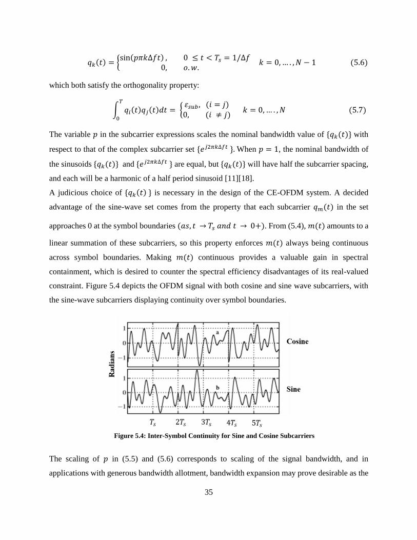
35
𝑞𝑘(𝑡) = {sin(𝑝𝜋𝑘∆𝑓𝑡) , 0 ≤ 𝑡 < 𝑇𝑠 = 1/∆𝑓
0, 𝑜. 𝑤. 𝑘 = 0, … . , 𝑁 − 1 (5.6)
which both satisfy the orthogonality property:
∫ 𝑞𝑖(𝑡)𝑞𝑗(𝑡)𝑑𝑡 = {휀𝑠𝑢𝑏 , (𝑖 = 𝑗)0, (𝑖 ≠ 𝑗)
𝑇
0
𝑘 = 0, … . , 𝑁 (5.7)
The variable 𝑝 in the subcarrier expressions scales the nominal bandwidth value of {𝑞𝑘(𝑡)} with
respect to that of the complex subcarrier set {𝑒𝑗2𝜋𝑘∆𝑓𝑡 }. When 𝑝 = 1, the nominal bandwidth of
the sinusoids {𝑞𝑘(𝑡)} and {𝑒𝑗2𝜋𝑘∆𝑓𝑡 } are equal, but {𝑞𝑘(𝑡)} will have half the subcarrier spacing,
and each will be a harmonic of a half period sinusoid [11][18].
A judicious choice of {𝑞𝑘(𝑡) } is necessary in the design of the CE-OFDM system. A decided
advantage of the sine-wave set comes from the property that each subcarrier 𝑞𝑚(𝑡) in the set
approaches 0 at the symbol boundaries (𝑎𝑠, 𝑡 → 𝑇𝑠 𝑎𝑛𝑑 𝑡 → 0+). From (5.4), 𝑚(𝑡) amounts to a
linear summation of these subcarriers, so this property enforces 𝑚(𝑡) always being continuous
across symbol boundaries. Making 𝑚(𝑡) continuous provides a valuable gain in spectral
containment, which is desired to counter the spectral efficiency disadvantages of its real-valued
constraint. Figure 5.4 depicts the OFDM signal with both cosine and sine wave subcarriers, with
the sine-wave subcarriers displaying continuity over symbol boundaries.
The scaling of 𝑝 in (5.5) and (5.6) corresponds to scaling of the signal bandwidth, and in
applications with generous bandwidth allotment, bandwidth expansion may prove desirable as the
Figure 5.4: Inter-Symbol Continuity for Sine and Cosine Subcarriers
36
phase modulated subcarrier symbols will be spread over a wider bandwidth providing the signal
greater frequency diversity.
5.3.3 Normalization Constant 𝐶𝑛:
𝐶𝑛 in (5.4) is a normalization constant which normalizes the variance of the modulated subcarriers
on the right-hand side of the expression. The variance, 𝜎𝑑, for equally-likely independent symbols
from an 𝑀-ary PAM constellation is given by 𝜎𝑑 =𝑀2−1
3. The expression for 𝐶𝑛 is then given by:
𝐶𝑛 = √2
𝑁𝜎𝑑2 =
3
𝑀2 − 1√
2
𝑁 (5.8)
5.3.4 Modulation Index 2𝜋ℎ:
The normalization constant 𝐶𝑛 allows the modulation index ℎ in Equation (5.4) to scale the
variance of the message signal, and the outer 2𝜋 coefficient converts this value into radians.
Increasing the value of ℎ increases the symbol energy in the message signal 𝑚(𝑡), and
correspondingly increases the Euclidean distance between the message symbols. Because the
expression in the double summation in Equation (5.4) is normalized by the constant 𝐶𝑛, regardless
of the modulation order of 𝐼𝑖,𝑘 , increasing the modulation index becomes necessary in order to
increase the Euclidean distance of the message symbols to accommodate higher order modulations.
The modulation index is a very important parameter of a CE-OFDM waveform, the choice of
which, as discussed in Section 5.5, has critical implications regarding both error-rate performance
and spectral containment of the CE-OFDM signal.
5.3.5 Memory Phases 𝜃𝑖:
Memory phases, 𝜃𝑖, in (5.4) are optional terms. These are constant phase offsets added to each CE-
OFDM symbol group in order to ensure continuous phase across symbol boundaries. The values
chosen for these memory phases are defined in Section 5.4.
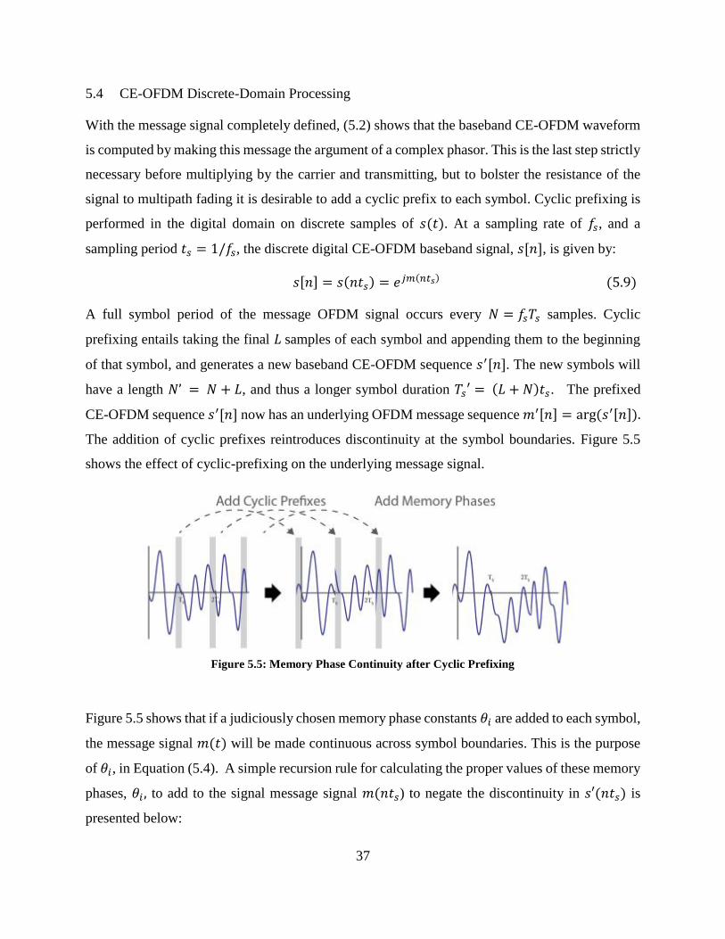
37
5.4 CE-OFDM Discrete-Domain Processing
With the message signal completely defined, (5.2) shows that the baseband CE-OFDM waveform
is computed by making this message the argument of a complex phasor. This is the last step strictly
necessary before multiplying by the carrier and transmitting, but to bolster the resistance of the
signal to multipath fading it is desirable to add a cyclic prefix to each symbol. Cyclic prefixing is
performed in the digital domain on discrete samples of 𝑠(𝑡). At a sampling rate of 𝑓𝑠, and a
sampling period 𝑡𝑠 = 1/𝑓𝑠, the discrete digital CE-OFDM baseband signal, 𝑠[𝑛], is given by:
𝑠[𝑛] = 𝑠(𝑛𝑡𝑠) = 𝑒𝑗𝑚(𝑛𝑡𝑠) (5.9)
A full symbol period of the message OFDM signal occurs every 𝑁 = 𝑓𝑠𝑇𝑠 samples. Cyclic
prefixing entails taking the final 𝐿 samples of each symbol and appending them to the beginning
of that symbol, and generates a new baseband CE-OFDM sequence 𝑠′[𝑛]. The new symbols will
have a length 𝑁’ = 𝑁 + 𝐿, and thus a longer symbol duration 𝑇𝑠′ = (𝐿 + 𝑁)𝑡𝑠. The prefixed
CE-OFDM sequence 𝑠′[𝑛] now has an underlying OFDM message sequence 𝑚′[𝑛] = arg (𝑠′[𝑛]).
The addition of cyclic prefixes reintroduces discontinuity at the symbol boundaries. Figure 5.5
shows the effect of cyclic-prefixing on the underlying message signal.
Figure 5.5 shows that if a judiciously chosen memory phase constants 𝜃𝑖 are added to each symbol,
the message signal 𝑚(𝑡) will be made continuous across symbol boundaries. This is the purpose
of 𝜃𝑖, in Equation (5.4). A simple recursion rule for calculating the proper values of these memory
phases, 𝜃𝑖 , to add to the signal message signal 𝑚(𝑛𝑡𝑠) to negate the discontinuity in 𝑠′(𝑛𝑡𝑠) is
presented below:
Figure 5.5: Memory Phase Continuity after Cyclic Prefixing
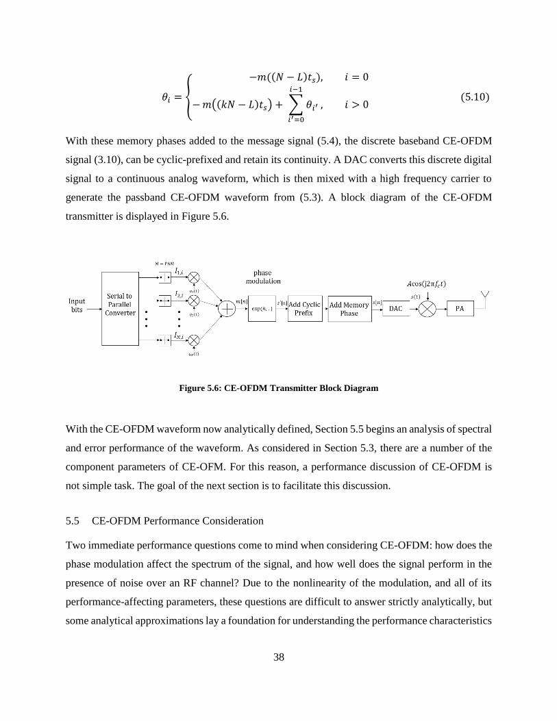
38
𝜃𝑖 = {
−𝑚((𝑁 − 𝐿)𝑡𝑠), 𝑖 = 0
− 𝑚((𝑘𝑁 − 𝐿)𝑡𝑠) + ∑ 𝜃𝑖′
𝑖−1
𝑖′=0
, 𝑖 > 0 (5.10)
With these memory phases added to the message signal (5.4), the discrete baseband CE-OFDM
signal (3.10), can be cyclic-prefixed and retain its continuity. A DAC converts this discrete digital
signal to a continuous analog waveform, which is then mixed with a high frequency carrier to
generate the passband CE-OFDM waveform from (5.3). A block diagram of the CE-OFDM
transmitter is displayed in Figure 5.6.
Figure 5.6: CE-OFDM Transmitter Block Diagram
With the CE-OFDM waveform now analytically defined, Section 5.5 begins an analysis of spectral
and error performance of the waveform. As considered in Section 5.3, there are a number of the
component parameters of CE-OFM. For this reason, a performance discussion of CE-OFDM is
not simple task. The goal of the next section is to facilitate this discussion.
5.5 CE-OFDM Performance Consideration
Two immediate performance questions come to mind when considering CE-OFDM: how does the
phase modulation affect the spectrum of the signal, and how well does the signal perform in the
presence of noise over an RF channel? Due to the nonlinearity of the modulation, and all of its
performance-affecting parameters, these questions are difficult to answer strictly analytically, but
some analytical approximations lay a foundation for understanding the performance characteristics
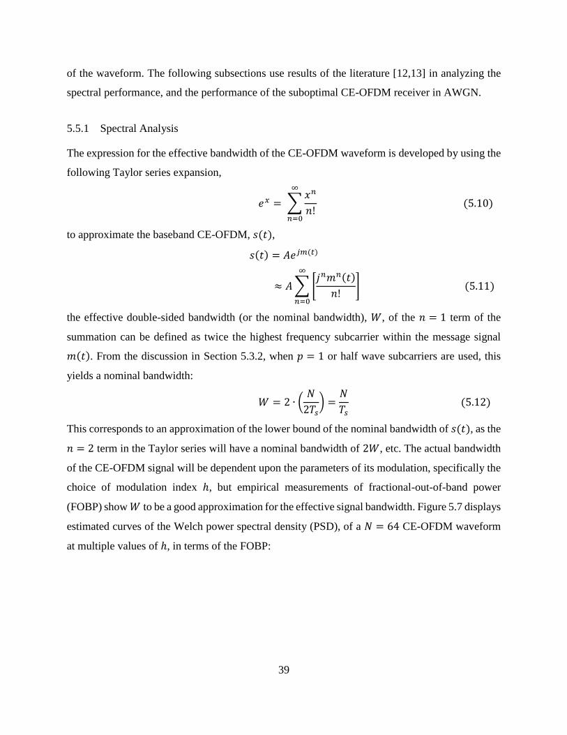
39
of the waveform. The following subsections use results of the literature [12,13] in analyzing the
spectral performance, and the performance of the suboptimal CE-OFDM receiver in AWGN.
5.5.1 Spectral Analysis
The expression for the effective bandwidth of the CE-OFDM waveform is developed by using the
following Taylor series expansion,
𝑒𝑥 = ∑𝑥𝑛
𝑛!
∞
𝑛=0
(5.10)
to approximate the baseband CE-OFDM, 𝑠(𝑡),
𝑠(𝑡) = 𝐴𝑒𝑗𝑚(𝑡)
≈ 𝐴 ∑ [𝑗𝑛𝑚𝑛(𝑡)
𝑛!] (5.11)
∞
𝑛=0
the effective double-sided bandwidth (or the nominal bandwidth), 𝑊, of the 𝑛 = 1 term of the
summation can be defined as twice the highest frequency subcarrier within the message signal
𝑚(𝑡). From the discussion in Section 5.3.2, when 𝑝 = 1 or half wave subcarriers are used, this
yields a nominal bandwidth:
𝑊 = 2 ∙ (𝑁
2𝑇𝑠) =
𝑁
𝑇𝑠 (5.12)
This corresponds to an approximation of the lower bound of the nominal bandwidth of 𝑠(𝑡), as the
𝑛 = 2 term in the Taylor series will have a nominal bandwidth of 2𝑊, etc. The actual bandwidth
of the CE-OFDM signal will be dependent upon the parameters of its modulation, specifically the
choice of modulation index ℎ, but empirical measurements of fractional-out-of-band power
(FOBP) show 𝑊 to be a good approximation for the effective signal bandwidth. Figure 5.7 displays
estimated curves of the Welch power spectral density (PSD), of a 𝑁 = 64 CE-OFDM waveform
at multiple values of ℎ, in terms of the FOBP:
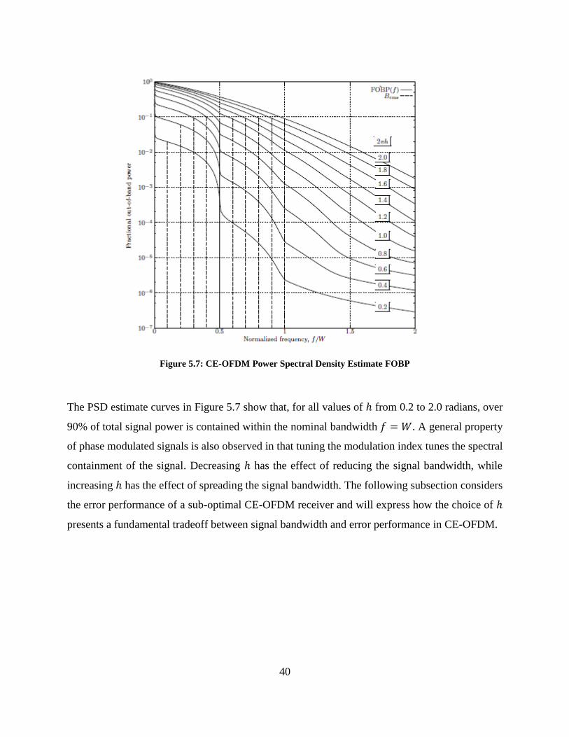
40
The PSD estimate curves in Figure 5.7 show that, for all values of ℎ from 0.2 to 2.0 radians, over
90% of total signal power is contained within the nominal bandwidth 𝑓 = 𝑊. A general property
of phase modulated signals is also observed in that tuning the modulation index tunes the spectral
containment of the signal. Decreasing ℎ has the effect of reducing the signal bandwidth, while
increasing ℎ has the effect of spreading the signal bandwidth. The following subsection considers
the error performance of a sub-optimal CE-OFDM receiver and will express how the choice of ℎ
presents a fundamental tradeoff between signal bandwidth and error performance in CE-OFDM.
Figure 5.7: CE-OFDM Power Spectral Density Estimate FOBP
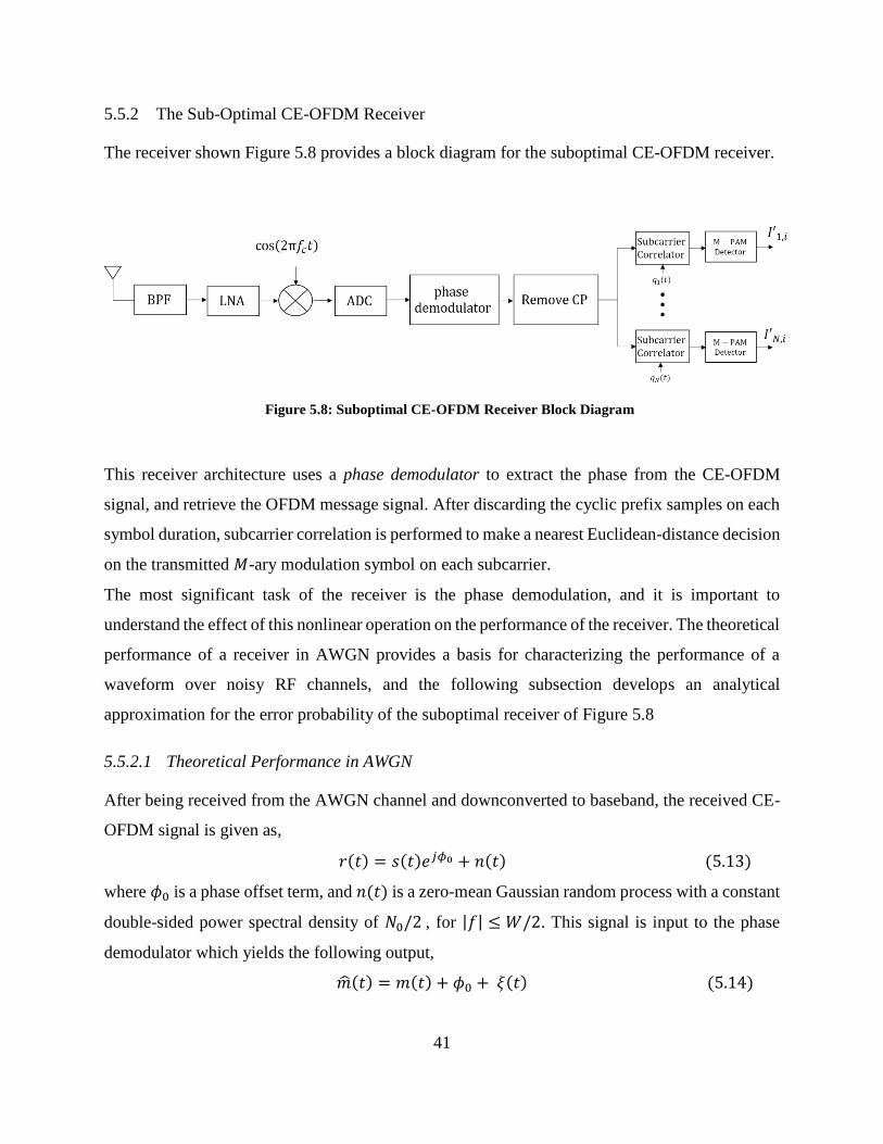
41
5.5.2 The Sub-Optimal CE-OFDM Receiver
The receiver shown Figure 5.8 provides a block diagram for the suboptimal CE-OFDM receiver.
This receiver architecture uses a phase demodulator to extract the phase from the CE-OFDM
signal, and retrieve the OFDM message signal. After discarding the cyclic prefix samples on each
symbol duration, subcarrier correlation is performed to make a nearest Euclidean-distance decision
on the transmitted 𝑀-ary modulation symbol on each subcarrier.
The most significant task of the receiver is the phase demodulation, and it is important to
understand the effect of this nonlinear operation on the performance of the receiver. The theoretical
performance of a receiver in AWGN provides a basis for characterizing the performance of a
waveform over noisy RF channels, and the following subsection develops an analytical
approximation for the error probability of the suboptimal receiver of Figure 5.8
5.5.2.1 Theoretical Performance in AWGN
After being received from the AWGN channel and downconverted to baseband, the received CE-
OFDM signal is given as,
𝑟(𝑡) = 𝑠(𝑡)𝑒𝑗𝜙0 + 𝑛(𝑡) (5.13)
where 𝜙0 is a phase offset term, and 𝑛(𝑡) is a zero-mean Gaussian random process with a constant
double-sided power spectral density of 𝑁0/2 , for |𝑓| ≤ 𝑊/2. This signal is input to the phase
demodulator which yields the following output,
�̂�(𝑡) = 𝑚(𝑡) + 𝜙0 + 𝜉(𝑡) (5.14)
Figure 5.8: Suboptimal CE-OFDM Receiver Block Diagram
42
where 𝑚(𝑡) is the original OFDM message signal, 𝜙0 is some constant phase offset, and 𝜉(𝑡) is
the phase component of the noise signal 𝑛(𝑡). If the carrier signal 𝐴𝑐𝑜𝑠(2𝜋𝑓𝑐𝑡) has an average
signal power 𝐴2 such that 𝐴2 ≫ 𝑁0, the phase demodulator output noise 𝜉(𝑡) will be
approximately linearly related with 𝑛(𝑡) and can be modeled as a zero-mean Gaussian noise
process with a power spectral density Φ𝜉(𝑓) given by,
Φ𝜉(𝑓) = 𝑁0/𝐴2, for |𝑓| ≤ 𝑊/2 (5.15)
This result, in which the carrier-to-noise ratio (CNR) of the phase demodulator can be modeled
as linearly related with the signal-to-noise ratio (SNR) of the demodulator output, is called the
high CNR approximation.
The phase demodulator output �̂�(𝑡) becomes the input to the bank of 𝑁 subcarrier correlators,
the output of each of which, taken over the symbol duration 𝑇𝑠, is given by,
𝑄𝑘 = ∫ �̂�(𝑡)𝑞𝑘(𝑡)𝑑𝑡
𝑇𝑠
0
= ∫{𝑚(𝑡) + 𝜙0 + 𝜉(𝑡) }𝑞𝑘(𝑡)𝑑𝑡
𝑇𝑠
0
≡ 𝑆𝑘 + Ψ𝑘 + 𝑁𝑘 (5.16)
which says that the output of the 𝑘𝑡ℎ subcarrier correlator will be composed of a message signal
component, 𝑆𝑘, a phase offset component, Ψ𝑘, and a phase noise component, 𝑁𝑘, which are
defined by,
𝑆𝑘 = ∫ 𝑚(𝑡)𝑞𝑘(𝑡)𝑑𝑡
𝑇𝑠
0
= ∫ {2𝜋ℎ𝐶𝑛 ∑ 𝐼𝑘′𝑞𝑘′(𝑡)
𝑁
𝑘′=1
+ 𝜃𝑖} 𝑞𝑘(𝑡)𝑑𝑡
𝑇𝑠
0
= ∫ 2𝜋ℎ𝐶𝑁
𝑇𝑠
0
∑ 𝐼𝑘′𝑞𝑘(𝑡)𝑞𝑘′(𝑡)
𝑁
𝑘′=1
𝑑𝑡
= 2𝜋ℎ𝐶𝑛𝐼𝑘 ∗ (𝑇𝑠
2)
= 2𝜋ℎ√(1/2)𝑁𝜎𝑑2 ∙ 𝐼𝑘 (5.17)
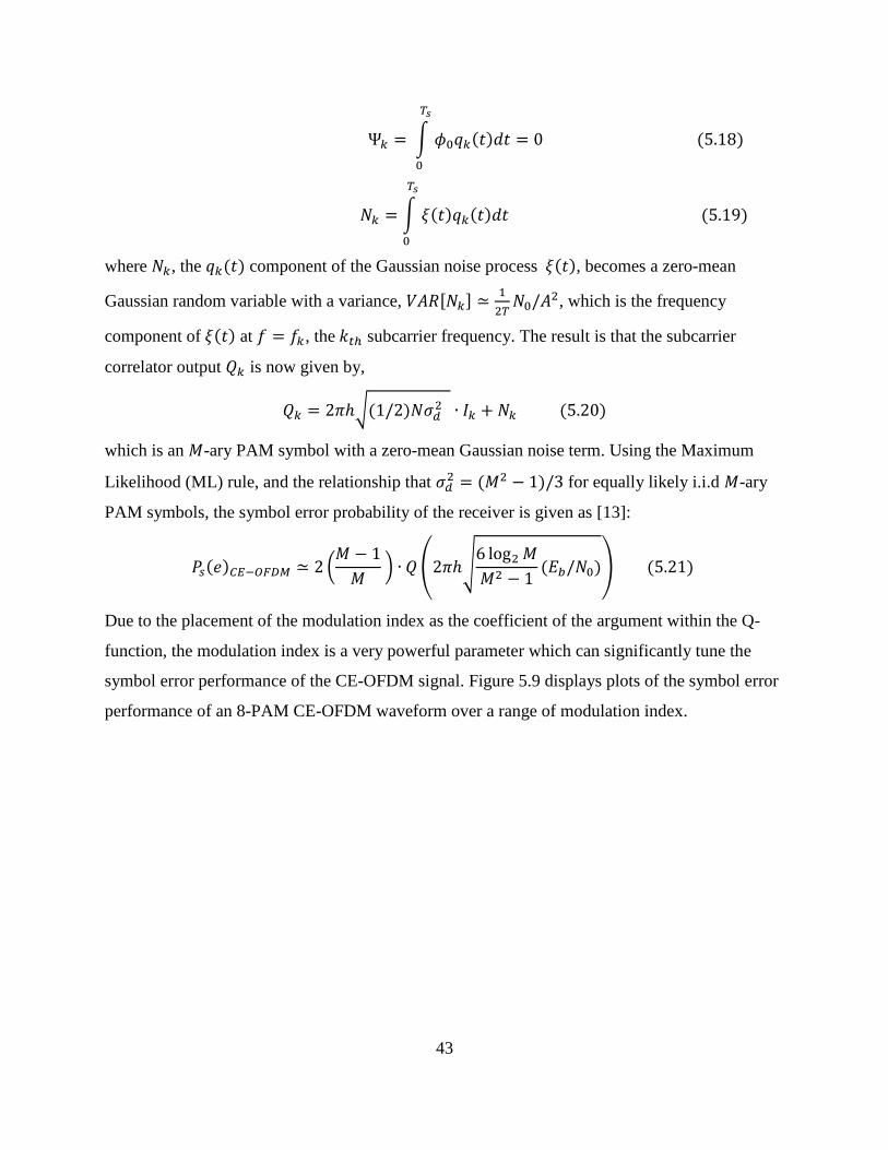
43
Ψ𝑘 = ∫ 𝜙0𝑞𝑘(𝑡)𝑑𝑡
𝑇𝑠
0
= 0 (5.18)
𝑁𝑘 = ∫ 𝜉(𝑡)𝑞𝑘(𝑡)𝑑𝑡 (5.19)
𝑇𝑠
0
where 𝑁𝑘, the 𝑞𝑘(𝑡) component of the Gaussian noise process 𝜉(𝑡), becomes a zero-mean
Gaussian random variable with a variance, 𝑉𝐴𝑅[𝑁𝑘] ≃1
2𝑇𝑁0/𝐴2, which is the frequency
component of 𝜉(𝑡) at 𝑓 = 𝑓𝑘, the 𝑘𝑡ℎ subcarrier frequency. The result is that the subcarrier
correlator output 𝑄𝑘 is now given by,
𝑄𝑘 = 2𝜋ℎ√(1/2)𝑁𝜎𝑑2 ∙ 𝐼𝑘 + 𝑁𝑘 (5.20)
which is an 𝑀-ary PAM symbol with a zero-mean Gaussian noise term. Using the Maximum
Likelihood (ML) rule, and the relationship that 𝜎𝑑2 = (𝑀2 − 1)/3 for equally likely i.i.d 𝑀-ary
PAM symbols, the symbol error probability of the receiver is given as [13]:
𝑃𝑠(𝑒)𝐶𝐸−𝑂𝐹𝐷𝑀 ≃ 2 (𝑀 − 1
𝑀 ) ∙ 𝑄 (2𝜋ℎ√
6 log2 𝑀
𝑀2 − 1(𝐸𝑏/𝑁0)) (5.21)
Due to the placement of the modulation index as the coefficient of the argument within the Q-
function, the modulation index is a very powerful parameter which can significantly tune the
symbol error performance of the CE-OFDM signal. Figure 5.9 displays plots of the symbol error
performance of an 8-PAM CE-OFDM waveform over a range of modulation index.

44
5.6 Critical Performance and Design Considerations
The brief analytical discussions of CE-OFDM spectral and error-rate performance provide a
foundation for understanding much of the character of the waveform. In this section a point-by-
point discussion of some of these traits is provided. The following subsection summarizes some
of the key challenges in the design of CE-OFDM systems and the subsequent subsection
summarizes the various merits of the CE-OFDM waveform.
5.6.1 The Challenges of CE-OFDM
While the result of Equation (5.21) describes the ideal error-rate performance of CE-OFDM, a few
practical considerations will make the performance deviate from this. One assumption made in the
derivation from Equation (5.14) is that the phase demodulator is able to recover a perfect copy of
the message signal with some additive noise interference term. The following subsections present
various factors which impact the performance of CE-OFDM, and challenge CE-OFDM design.
Figure 5.9: CE-OFDM Symbol Error Rate vs SNR vs various 𝟐𝝅𝒉
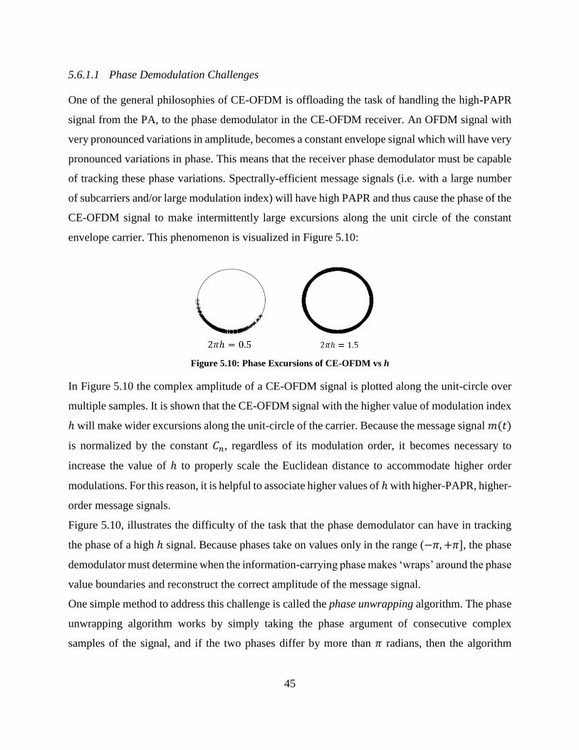
45
5.6.1.1 Phase Demodulation Challenges
One of the general philosophies of CE-OFDM is offloading the task of handling the high-PAPR
signal from the PA, to the phase demodulator in the CE-OFDM receiver. An OFDM signal with
very pronounced variations in amplitude, becomes a constant envelope signal which will have very
pronounced variations in phase. This means that the receiver phase demodulator must be capable
of tracking these phase variations. Spectrally-efficient message signals (i.e. with a large number
of subcarriers and/or large modulation index) will have high PAPR and thus cause the phase of the
CE-OFDM signal to make intermittently large excursions along the unit circle of the constant
envelope carrier. This phenomenon is visualized in Figure 5.10:
In Figure 5.10 the complex amplitude of a CE-OFDM signal is plotted along the unit-circle over
multiple samples. It is shown that the CE-OFDM signal with the higher value of modulation index
ℎ will make wider excursions along the unit-circle of the carrier. Because the message signal 𝑚(𝑡)
is normalized by the constant 𝐶𝑛, regardless of its modulation order, it becomes necessary to
increase the value of ℎ to properly scale the Euclidean distance to accommodate higher order
modulations. For this reason, it is helpful to associate higher values of ℎ with higher-PAPR, higher-
order message signals.
Figure 5.10, illustrates the difficulty of the task that the phase demodulator can have in tracking
the phase of a high ℎ signal. Because phases take on values only in the range (−𝜋, +𝜋], the phase
demodulator must determine when the information-carrying phase makes ‘wraps’ around the phase
value boundaries and reconstruct the correct amplitude of the message signal.
One simple method to address this challenge is called the phase unwrapping algorithm. The phase
unwrapping algorithm works by simply taking the phase argument of consecutive complex
samples of the signal, and if the two phases differ by more than 𝜋 radians, then the algorithm
Figure 5.10: Phase Excursions of CE-OFDM vs h
46
determines that the phase has ‘wrapped’ over a phase boundary and ‘unwraps’ this by adding ±𝜋
radians to the next sample.
The phase unwrapping algorithm expects that the phase of the signal will make gentle excursions
along the unit-circle and thus will be very effective for signals with low ℎ and high SNR. However,
signals with high ℎ and/or high phase noise will commonly make wide swings in phase along the
unit-circle, and if these swings are greater than 𝜋 radians over one sampling interval then the
unwrapper algorithm will make ‘false wrap’ errors, which will cause degraded performance. The
false wrap errors of the phase unwrapper can be reduced with the use of high oversampling value,
such that the sampling interval is small enough to track very fast excursions of the phase, and also
employing appropriate filtering to remove any out-of-band noise components before the task of
phase demodulation. More advanced techniques for phase tracking are possible with some added
complexity. These include phase-locked-loop (PLL) and cyclic-slip estimation (CSE) [22].
5.6.1.2 The FM Threshold Problem
Angle modulation, whether FM or PM, experiences the phenomenon called FM thresholding.
When the CNR of the angle-modulated CE-OFDM signal drops below 10 dB, the linear
relationship between the CNR of the received signal and the SNR at the output of the phase
demodulator fails, resulting in an increase in phase noise which will cause the message signal to
become critically obscured by phase noise. Below the FM threshold, the phase demodulator will
not be able to properly track the highly unstable phase, resulting in phase demodulator error, and
the message signal, even if correctly extracted, becomes too obscured by error to decode.
Techniques to extend the FM threshold range exist [22], but CE-OFDM system designers should
be careful to avoid operation below 10 dB CNR in order to aid phase tracking and message signal
detection in the phase demodulator receiver.
5.6.1.3 Real Message Signal Requirement
As discussed in Section 5.3.2, the phase modulator message signal is required to be purely real,
and this requires the CE-OFDM subcarriers to be purely real. For this reason, twice the number of
subcarriers, with half the subcarrier separation, is required for CE-OFDM to provide the same
nominal bandwidth as OFDM. In the context of multicarrier communications, condensing
subcarrier separation naturally raises some concerns regarding maintaining subcarrier
47
orthogonality, but as is discussed in the strengths section to come, this concern is mitigated in CE-
OFDM. The more poignant issue with the real-message signal requirement is that it constrains
subcarrier modulations to be of the 1-dimensional, 𝑀-ary PAM variety which certainly restricts
the spectral efficiency of CE-OFDM in comparison to OFDM, whose subcarriers can be modulated
by any symbols on a 2-dimensonial constellation.
5.6.1.4 Multiple Access and Standards Integration
One challenging engineering problem will be the integration of CE-OFDM waveforms into present
OFDM-based standards. The linearity and subcarrier orthogonality of OFDM which enables the
OFDMA multiple access scheme is no longer present in CE-OFDM. For instance, two users
transmitting CE-OFDM simultaneously in a channel would incur interference on each other
regardless of which message signal subcarriers were modulated. This means that traditional forms
of single-carrier multiple access techniques may be required for CE-OFDM systems, a restriction
which diverges from the trend of next generation wireless communications. Some intelligent
engineering would be required to adapt CE-OFDM into the next generation standards.
5.6.2 The Strengths of CE-OFDM
CE-OFDM is a single-carrier modulation scheme which takes on much of the nature of a multi-
carrier modulation scheme. The modulation scheme transmits symbols in parallel over a
wideband channel, but it does so on a single carrier. The phase modulation can then be
considered as a non-linear spreading or ‘smearing’ of the multicarrier signal, which is recovered
by the phase demodulator. In this way, CE-OFDM retains the critical characteristics of a
multicarrier signal, with a few additional benefits:
5.6.2.1 ISI-Immunity
As described in Section 5.4, the addition of a cyclic prefix to a CE-OFDM symbol block has the
identical purpose and effect as in standard OFDM. With small overhead in symbol time to a long
duration CE-OFDM symbol, the cyclic prefix effectively mitigates ISI. Like OFDM, CE-OFDM
requires only simple equalization and can make use of single-carrier frequency-domain
equalization (SC-FDE) techniques.
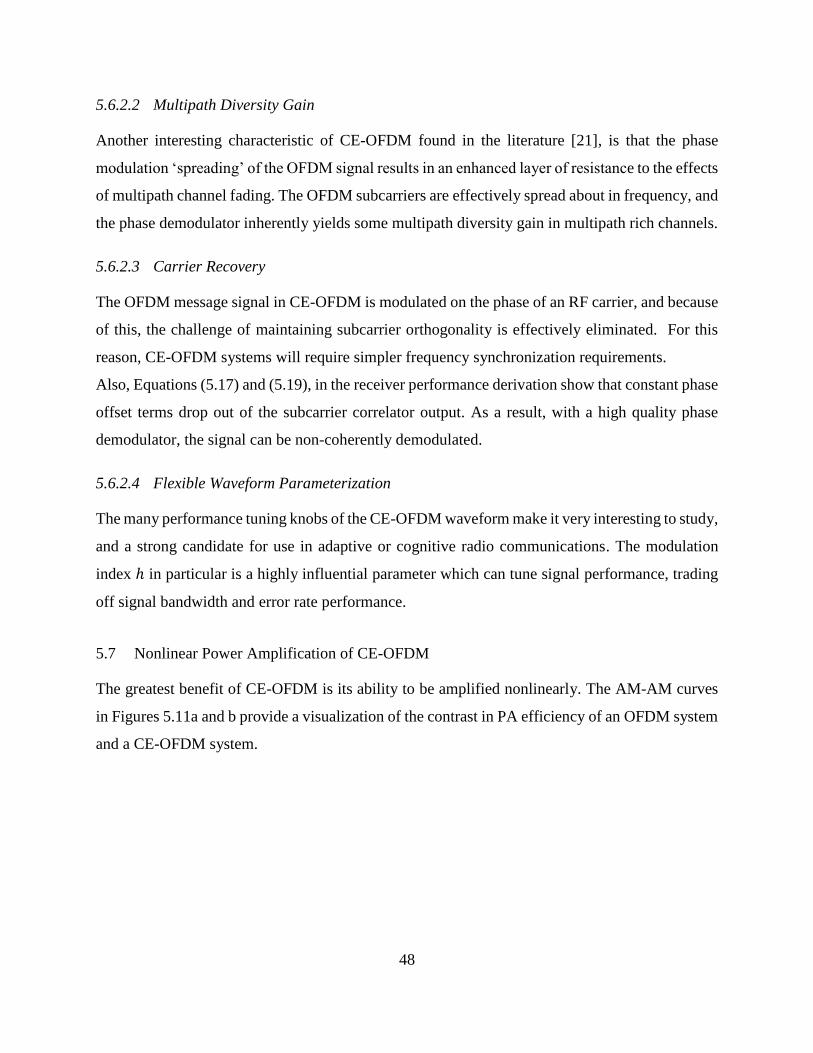
48
5.6.2.2 Multipath Diversity Gain
Another interesting characteristic of CE-OFDM found in the literature [21], is that the phase
modulation ‘spreading’ of the OFDM signal results in an enhanced layer of resistance to the effects
of multipath channel fading. The OFDM subcarriers are effectively spread about in frequency, and
the phase demodulator inherently yields some multipath diversity gain in multipath rich channels.
5.6.2.3 Carrier Recovery
The OFDM message signal in CE-OFDM is modulated on the phase of an RF carrier, and because
of this, the challenge of maintaining subcarrier orthogonality is effectively eliminated. For this
reason, CE-OFDM systems will require simpler frequency synchronization requirements.
Also, Equations (5.17) and (5.19), in the receiver performance derivation show that constant phase
offset terms drop out of the subcarrier correlator output. As a result, with a high quality phase
demodulator, the signal can be non-coherently demodulated.
5.6.2.4 Flexible Waveform Parameterization
The many performance tuning knobs of the CE-OFDM waveform make it very interesting to study,
and a strong candidate for use in adaptive or cognitive radio communications. The modulation
index ℎ in particular is a highly influential parameter which can tune signal performance, trading
off signal bandwidth and error rate performance.
5.7 Nonlinear Power Amplification of CE-OFDM
The greatest benefit of CE-OFDM is its ability to be amplified nonlinearly. The AM-AM curves
in Figures 5.11a and b provide a visualization of the contrast in PA efficiency of an OFDM system
and a CE-OFDM system.
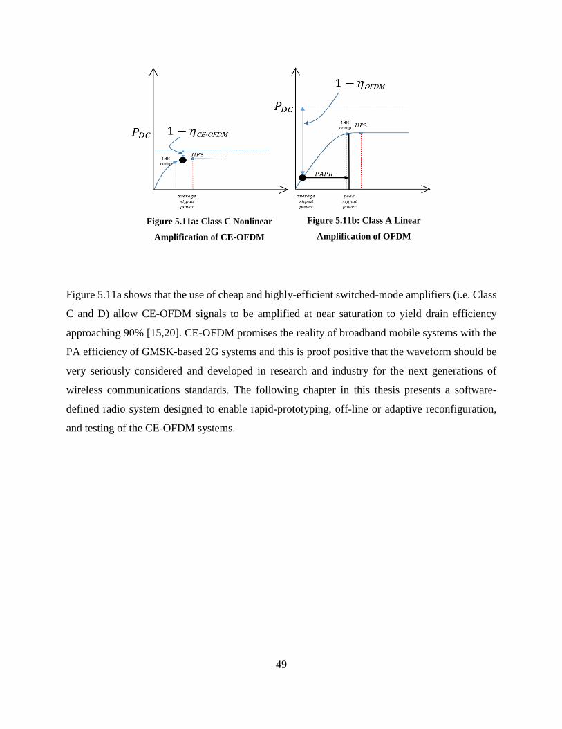
49
Figure 5.11a shows that the use of cheap and highly-efficient switched-mode amplifiers (i.e. Class
C and D) allow CE-OFDM signals to be amplified at near saturation to yield drain efficiency
approaching 90% [15,20]. CE-OFDM promises the reality of broadband mobile systems with the
PA efficiency of GMSK-based 2G systems and this is proof positive that the waveform should be
very seriously considered and developed in research and industry for the next generations of
wireless communications standards. The following chapter in this thesis presents a software-
defined radio system designed to enable rapid-prototyping, off-line or adaptive reconfiguration,
and testing of the CE-OFDM systems.
Figure 5.11a: Class C Nonlinear
Amplification of CE-OFDM
Figure 5.11b: Class A Linear
Amplification of OFDM
50
6 SDR IMPLEMENTATION OF CE-OFDM WAVEFORM
The CE-OFDM waveform has been presented in the previous chapter as a novel technique for
optimal PAPR reduction in OFDM systems. The waveform has a number of interesting
properties and performance-affecting parameters. To study these, an SDR implementation of a
rapid-prototypable CE-OFDM system has been adopted. Details of the GNU Radio SDR
development framework are presented in Section 1, and Sections 6.2 and 6.3 of detail the
software implementation of the CE-OFDM transmitter and receiver.
6.1 GNU Radio SDR Development
GNU Radio is an open-source, highly extensible software framework for developing SDR
applications and waveforms on a GPP. The key components of the GNU Radio software
framework are defined in the subsections that follow:
6.1.1 Signal Processing Blocks
In GNU Radio, signal processing blocks are modular structures, written in C++ or Python,
which use signal processing algorithms to process digital signal samples. Signal processing blocks
are the fundamental components of waveforms. Source and sink blocks form the bookends of a
GNU Radio ‘flowgraph’.
Source blocks are signal processing blocks which have outputs but no inputs, and generate
the samples of a digital signal at the input of the GNU Radio waveform. Software source blocks
use software routines to generate and stream digital signal samples into the GNU Radio waveform.
Hardware source blocks set up hardware drivers or network sockets to stream digital signal
samples from hardware sources such as computer soundcards, UDP or TCP network applications,
and RF front ends such as USRPs, into the GNU Radio waveform.
Sink blocks are signal processing blocks that have inputs but no outputs. They consume
digital samples at the output of the GNU Radio waveform. Software sink blocks in GNU Radio
include a number of graphical user interface (GUI) modules which provide a graphical display of
51
input data samples. Hardware sink blocks use hardware drivers or network sockets to stream digital
signal samples out of GNU Radio waveforms and into hardware devices.
6.1.2 GNU Radio Scheduler
The GNU Radio Scheduler is the heart of the GNU Radio system. When a flowgraph is
executing, the GNU Radio Scheduler buffers and cycles digital samples into and out of each block
in the waveform, enabling the GPP to perform real-time baseband modulation and demodulation.
6.1.3 Python Programmatic Interface
The primary interface to the GNU Radio framework is the Python language. Python
provides a clean and simple interface to the GNU Radio system and abstracts away details of
memory management from the programmer. Once GNU Radio libraries are imported, all GNU
Radio blocks become accessible in Python. This allows a programmer to implement GNU Radio
flowgraphs by instantiating all blocks in the flowgraph, by connecting them in a ‘top block’ object.
When the ‘run’ method of the top block object is called, the GNU Radio scheduler will begin real-
time processing of the user-defined flowgraph.
6.1.4 GNU Radio Companion Graphical Interface
GNU Radio also provides a graphical user interface (GUI), called GNU Radio Companion
(GRC) to accompany its Python programmatic interface. In GRC the user can instantiate GNU
Radio blocks graphically by dragging and dropping graphical blocks onto a workspace and
chaining them together to form a flowgraph. Upon execution of the graphical flowgraph, an
underlying Python script is generated and executed to begin real-time processing of the flowgraph.
6.1.5 Creating Custom GNU Radio Blocks
The extensibility of the GNU Radio system is founded on the object-oriented programming
(OOP) principle of inheritance. In the inheritance principle, one object, called a child, inherits the
attributes of another object, called a parent. Custom blocks or modules in GNU Radio inherit a
software structure as illustrated in Figure 6.1.
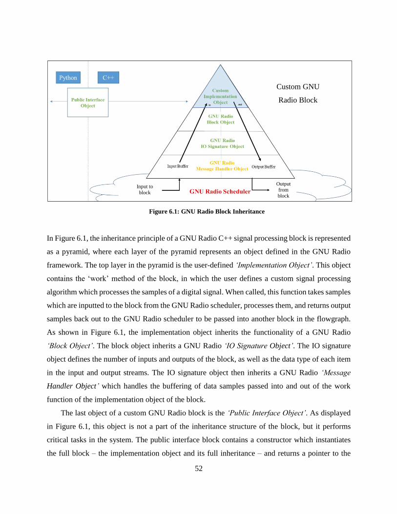
52
In Figure 6.1, the inheritance principle of a GNU Radio C++ signal processing block is represented
as a pyramid, where each layer of the pyramid represents an object defined in the GNU Radio
framework. The top layer in the pyramid is the user-defined ‘Implementation Object’. This object
contains the ‘work’ method of the block, in which the user defines a custom signal processing
algorithm which processes the samples of a digital signal. When called, this function takes samples
which are inputted to the block from the GNU Radio scheduler, processes them, and returns output
samples back out to the GNU Radio scheduler to be passed into another block in the flowgraph.
As shown in Figure 6.1, the implementation object inherits the functionality of a GNU Radio
‘Block Object’. The block object inherits a GNU Radio ‘IO Signature Object’. The IO signature
object defines the number of inputs and outputs of the block, as well as the data type of each item
in the input and output streams. The IO signature object then inherits a GNU Radio ‘Message
Handler Object’ which handles the buffering of data samples passed into and out of the work
function of the implementation object of the block.
The last object of a custom GNU Radio block is the ‘Public Interface Object’. As displayed
in Figure 6.1, this object is not a part of the inheritance structure of the block, but it performs
critical tasks in the system. The public interface block contains a constructor which instantiates
the full block – the implementation object and its full inheritance – and returns a pointer to the
Figure 6.1: GNU Radio Block Inheritance
Custom GNU
Radio Block
Input to
block
Output
from
block
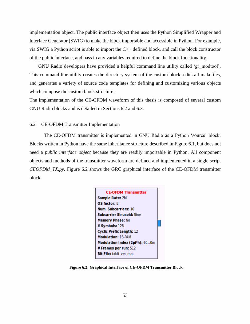
53
implementation object. The public interface object then uses the Python Simplified Wrapper and
Interface Generator (SWIG) to make the block importable and accessible in Python. For example,
via SWIG a Python script is able to import the C++ defined block, and call the block constructor
of the public interface, and pass in any variables required to define the block functionality.
GNU Radio developers have provided a helpful command line utility called ‘gr_modtool’.
This command line utility creates the directory system of the custom block, edits all makefiles,
and generates a variety of source code templates for defining and customizing various objects
which compose the custom block structure.
The implementation of the CE-OFDM waveform of this thesis is composed of several custom
GNU Radio blocks and is detailed in Sections 6.2 and 6.3.
6.2 CE-OFDM Transmitter Implementation
The CE-OFDM transmitter is implemented in GNU Radio as a Python ‘source’ block.
Blocks written in Python have the same inheritance structure described in Figure 6.1, but does not
need a public interface object because they are readily importable in Python. All component
objects and methods of the transmitter waveform are defined and implemented in a single script
CEOFDM_TX.py. Figure 6.2 shows the GRC graphical interface of the CE-OFDM transmitter
block.
Figure 6.2: Graphical Interface of CE-OFDM Transmitter Block
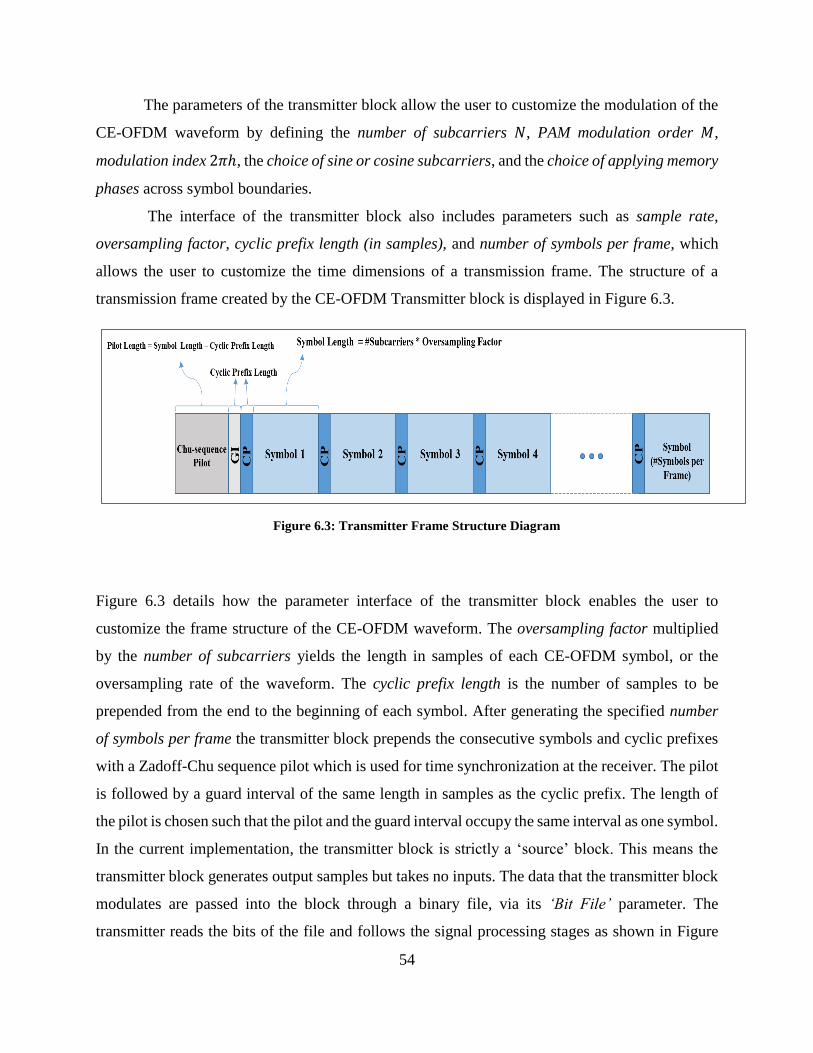
54
The parameters of the transmitter block allow the user to customize the modulation of the
CE-OFDM waveform by defining the number of subcarriers 𝑁, PAM modulation order 𝑀,
modulation index 2𝜋ℎ, the choice of sine or cosine subcarriers, and the choice of applying memory
phases across symbol boundaries.
The interface of the transmitter block also includes parameters such as sample rate,
oversampling factor, cyclic prefix length (in samples), and number of symbols per frame, which
allows the user to customize the time dimensions of a transmission frame. The structure of a
transmission frame created by the CE-OFDM Transmitter block is displayed in Figure 6.3.
Figure 6.3 details how the parameter interface of the transmitter block enables the user to
customize the frame structure of the CE-OFDM waveform. The oversampling factor multiplied
by the number of subcarriers yields the length in samples of each CE-OFDM symbol, or the
oversampling rate of the waveform. The cyclic prefix length is the number of samples to be
prepended from the end to the beginning of each symbol. After generating the specified number
of symbols per frame the transmitter block prepends the consecutive symbols and cyclic prefixes
with a Zadoff-Chu sequence pilot which is used for time synchronization at the receiver. The pilot
is followed by a guard interval of the same length in samples as the cyclic prefix. The length of
the pilot is chosen such that the pilot and the guard interval occupy the same interval as one symbol.
In the current implementation, the transmitter block is strictly a ‘source’ block. This means the
transmitter block generates output samples but takes no inputs. The data that the transmitter block
modulates are passed into the block through a binary file, via its ‘Bit File’ parameter. The
transmitter reads the bits of the file and follows the signal processing stages as shown in Figure
Figure 6.3: Transmitter Frame Structure Diagram
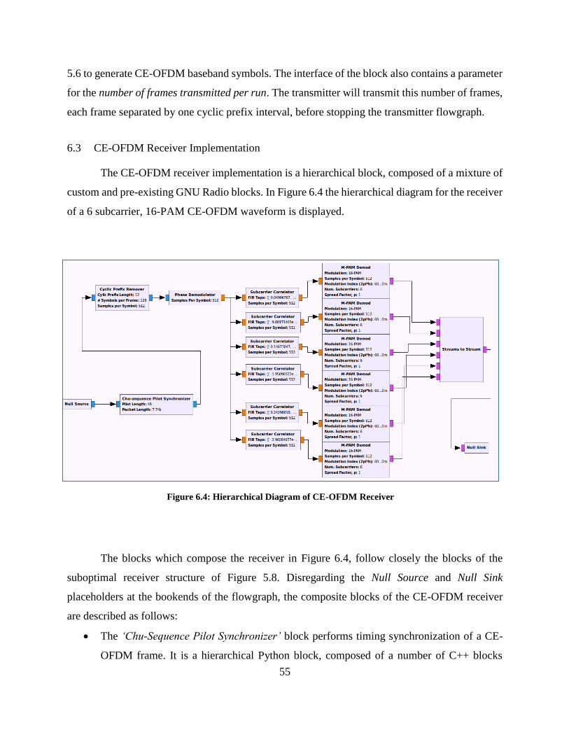
55
5.6 to generate CE-OFDM baseband symbols. The interface of the block also contains a parameter
for the number of frames transmitted per run. The transmitter will transmit this number of frames,
each frame separated by one cyclic prefix interval, before stopping the transmitter flowgraph.
6.3 CE-OFDM Receiver Implementation
The CE-OFDM receiver implementation is a hierarchical block, composed of a mixture of
custom and pre-existing GNU Radio blocks. In Figure 6.4 the hierarchical diagram for the receiver
of a 6 subcarrier, 16-PAM CE-OFDM waveform is displayed.
The blocks which compose the receiver in Figure 6.4, follow closely the blocks of the
suboptimal receiver structure of Figure 5.8. Disregarding the Null Source and Null Sink
placeholders at the bookends of the flowgraph, the composite blocks of the CE-OFDM receiver
are described as follows:
The ‘Chu-Sequence Pilot Synchronizer’ block performs timing synchronization of a CE-
OFDM frame. It is a hierarchical Python block, composed of a number of C++ blocks
Figure 6.4: Hierarchical Diagram of CE-OFDM Receiver
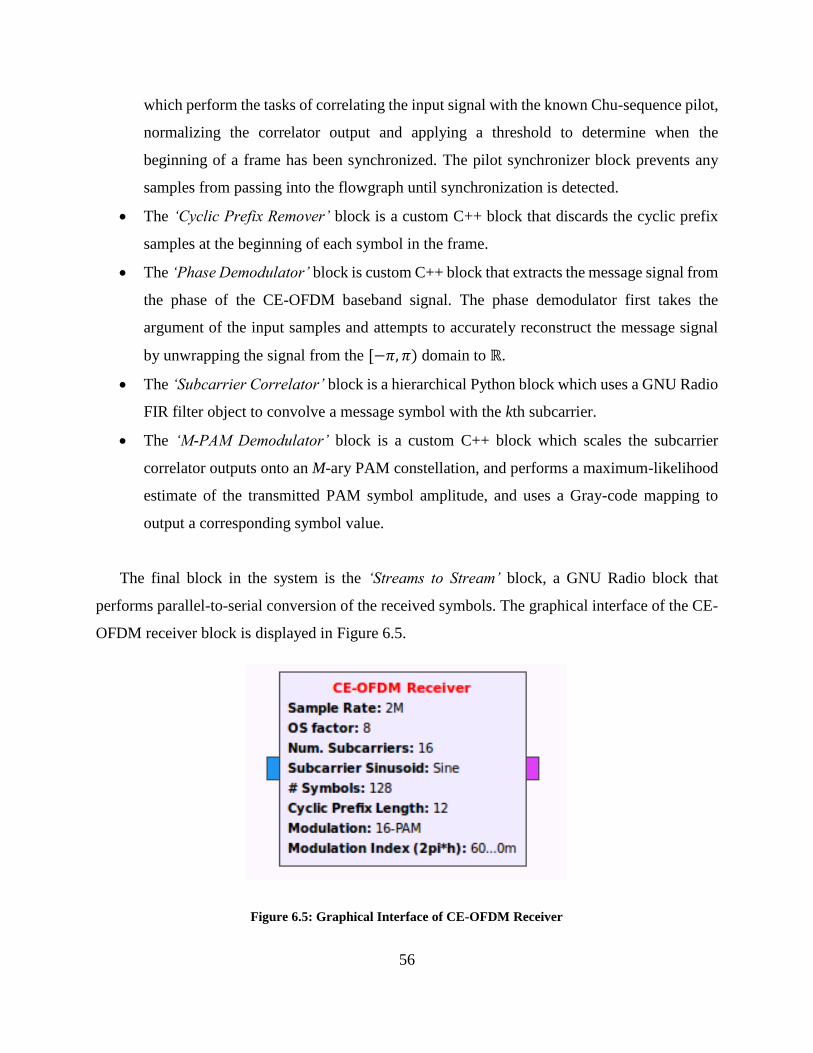
56
which perform the tasks of correlating the input signal with the known Chu-sequence pilot,
normalizing the correlator output and applying a threshold to determine when the
beginning of a frame has been synchronized. The pilot synchronizer block prevents any
samples from passing into the flowgraph until synchronization is detected.
The ‘Cyclic Prefix Remover’ block is a custom C++ block that discards the cyclic prefix
samples at the beginning of each symbol in the frame.
The ‘Phase Demodulator’ block is custom C++ block that extracts the message signal from
the phase of the CE-OFDM baseband signal. The phase demodulator first takes the
argument of the input samples and attempts to accurately reconstruct the message signal
by unwrapping the signal from the [−𝜋, 𝜋) domain to ℝ.
The ‘Subcarrier Correlator’ block is a hierarchical Python block which uses a GNU Radio
FIR filter object to convolve a message symbol with the kth subcarrier.
The ‘M-PAM Demodulator’ block is a custom C++ block which scales the subcarrier
correlator outputs onto an M-ary PAM constellation, and performs a maximum-likelihood
estimate of the transmitted PAM symbol amplitude, and uses a Gray-code mapping to
output a corresponding symbol value.
The final block in the system is the ‘Streams to Stream’ block, a GNU Radio block that
performs parallel-to-serial conversion of the received symbols. The graphical interface of the CE-
OFDM receiver block is displayed in Figure 6.5.
Figure 6.5: Graphical Interface of CE-OFDM Receiver
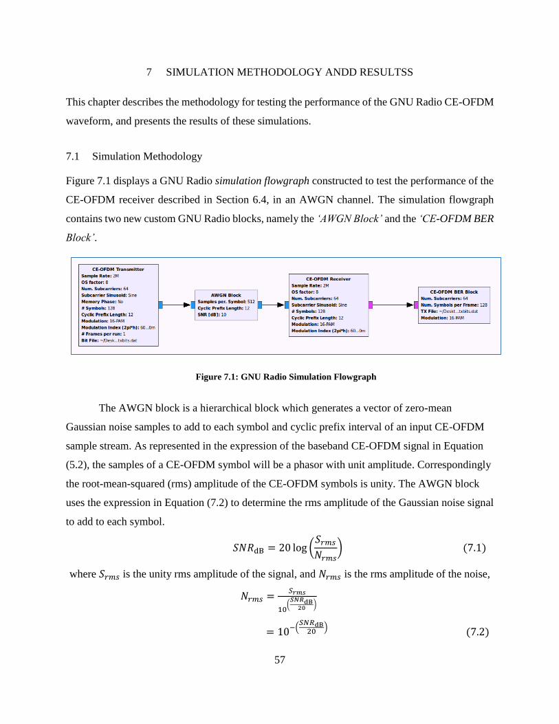
57
7 SIMULATION METHODOLOGY ANDD RESULTSS
This chapter describes the methodology for testing the performance of the GNU Radio CE-OFDM
waveform, and presents the results of these simulations.
7.1 Simulation Methodology
Figure 7.1 displays a GNU Radio simulation flowgraph constructed to test the performance of the
CE-OFDM receiver described in Section 6.4, in an AWGN channel. The simulation flowgraph
contains two new custom GNU Radio blocks, namely the ‘AWGN Block’ and the ‘CE-OFDM BER
Block’.
The AWGN block is a hierarchical block which generates a vector of zero-mean
Gaussian noise samples to add to each symbol and cyclic prefix interval of an input CE-OFDM
sample stream. As represented in the expression of the baseband CE-OFDM signal in Equation
(5.2), the samples of a CE-OFDM symbol will be a phasor with unit amplitude. Correspondingly
the root-mean-squared (rms) amplitude of the CE-OFDM symbols is unity. The AWGN block
uses the expression in Equation (7.2) to determine the rms amplitude of the Gaussian noise signal
to add to each symbol.
𝑆𝑁𝑅dB = 20 log (𝑆𝑟𝑚𝑠
𝑁𝑟𝑚𝑠) (7.1)
where 𝑆𝑟𝑚𝑠 is the unity rms amplitude of the signal, and 𝑁𝑟𝑚𝑠 is the rms amplitude of the noise,
𝑁𝑟𝑚𝑠 =𝑆𝑟𝑚𝑠
10(
𝑆𝑁𝑅dB20
)
= 10−(𝑆𝑁𝑅dB
20) (7.2)
Figure 7.1: GNU Radio Simulation Flowgraph
58
The AWGN block utilizes the GNU Radio ‘Gaussian Noise Source’ block to generate a
Gaussian noise with the rms amplitude given in Equation (7.2), for a value of signal-to-noise
ratio (SNR) specified at the interface of the AWGN block.
The output of the AWGN block in Figure 7.1 is a noisy CE-OFDM signal which is input to the
CE-OFDM receiver. The final block in the simulation flowgraph is the CE-OFDM BER block,
which receives the demodulated symbols from the CE-OFDM receiver and reads the same binary
file from which the transmitter modulates its frames, to calculate the bit-error rate (BER)
performance of the system.
The flowgraph in Figure 7.1 is the graphical representation of a GNU Radio ‘top block’ object
which forms a ‘testbench’ for testing the CE-OFDM waveform. The testbench is coded with
interface parameters to allow the user to configure various parameters of the waveform, the noise
level of the AWGN channel, simulate the transmission and reception of 1 million bits CE-OFDM
frames, and retrieve the bit error rate (BER) results of the simulation. Figure 7.2 displays an
excerpt of Python script which will execute the testbench object over multiple noise levels of the
AWGN channel and multiple configurations of the modulation index, number of subcarriers, and
𝑀-ary PAM modulation order of the CE-OFDM waveform.
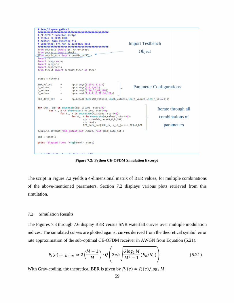
59
The script in Figure 7.2 yields a 4-dimensional matrix of BER values, for multiple combinations
of the above-mentioned parameters. Section 7.2 displays various plots retrieved from this
simulation.
7.2 Simulation Results
The Figures 7.3 through 7.6 display BER versus SNR waterfall curves over multiple modulation
indices. The simulated curves are plotted against curves derived from the theoretical symbol error
rate approximation of the sub-optimal CE-OFDM receiver in AWGN from Equation (5.21).
𝑃𝑠(𝑒)𝐶𝐸−𝑂𝐹𝐷𝑀 ≃ 2 (𝑀 − 1
𝑀 ) ∙ 𝑄 (2𝜋ℎ√
6 log2 𝑀
𝑀2 − 1(𝐸𝑏/𝑁0)) (5.21)
With Gray-coding, the theoretical BER is given by 𝑃𝑏(𝑒) ≃ 𝑃𝑠(𝑒) log2 𝑀⁄ .
Figure 7.2: Python CE-OFDM Simulation Excerpt
Import Testbench
Object
Parameter Configurations
Iterate through all
combinations of
parameters
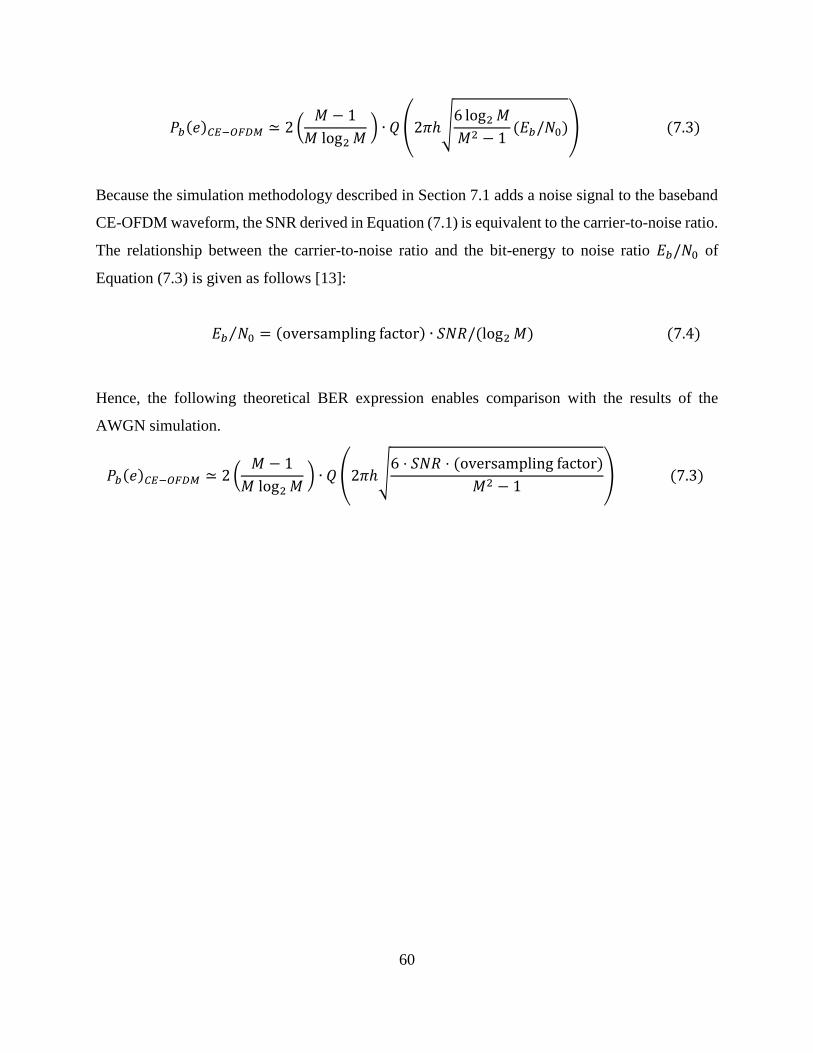
60
𝑃𝑏(𝑒)𝐶𝐸−𝑂𝐹𝐷𝑀 ≃ 2 (𝑀 − 1
𝑀 log2 𝑀 ) ∙ 𝑄 (2𝜋ℎ√
6 log2 𝑀
𝑀2 − 1(𝐸𝑏/𝑁0)) (7.3)
Because the simulation methodology described in Section 7.1 adds a noise signal to the baseband
CE-OFDM waveform, the SNR derived in Equation (7.1) is equivalent to the carrier-to-noise ratio.
The relationship between the carrier-to-noise ratio and the bit-energy to noise ratio 𝐸𝑏/𝑁0 of
Equation (7.3) is given as follows [13]:
𝐸𝑏 𝑁0⁄ = (oversampling factor) ∙ 𝑆𝑁𝑅/(log2 𝑀) (7.4)
Hence, the following theoretical BER expression enables comparison with the results of the
AWGN simulation.
𝑃𝑏(𝑒)𝐶𝐸−𝑂𝐹𝐷𝑀 ≃ 2 (𝑀 − 1
𝑀 log2 𝑀 ) ∙ 𝑄 (2𝜋ℎ√
6 ⋅ 𝑆𝑁𝑅 ⋅ (oversampling factor)
𝑀2 − 1) (7.3)
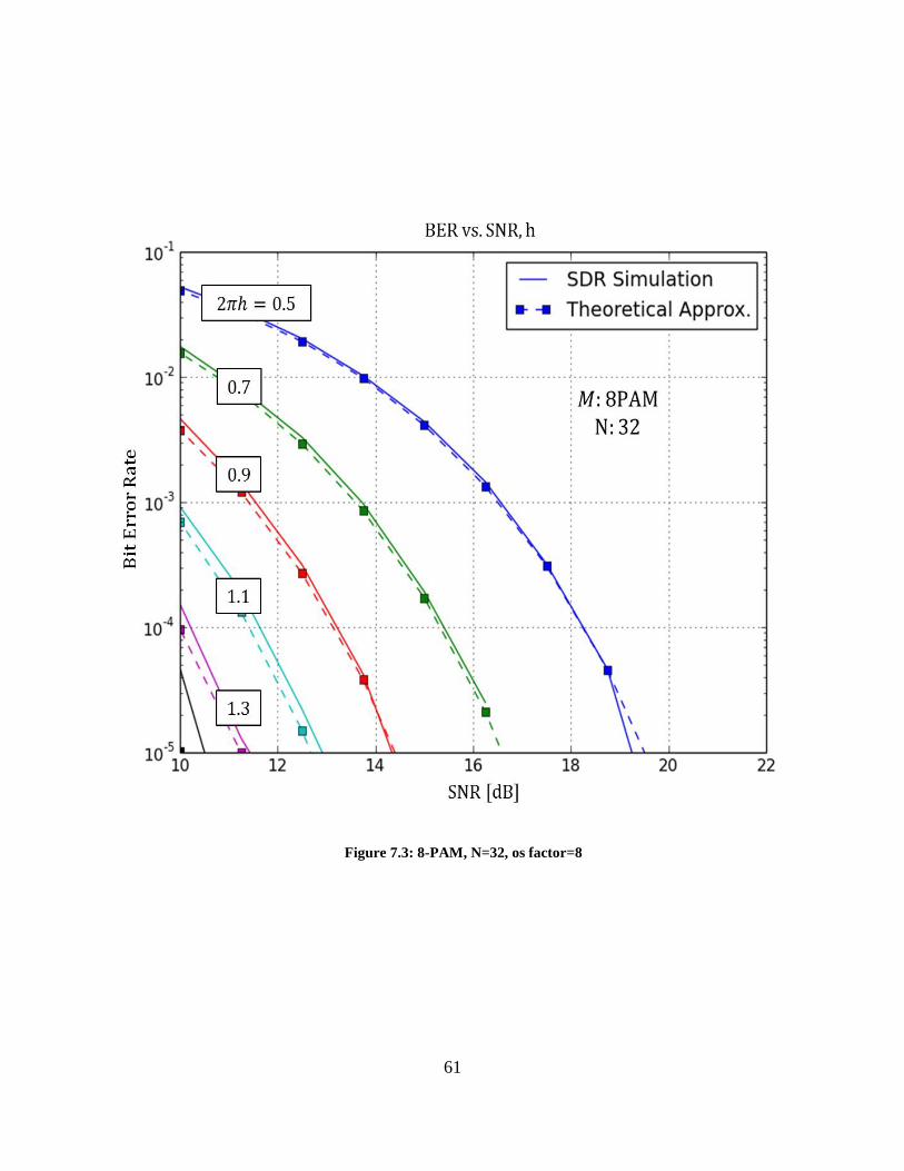
61
Figure 7.3: 8-PAM, N=32, os factor=8
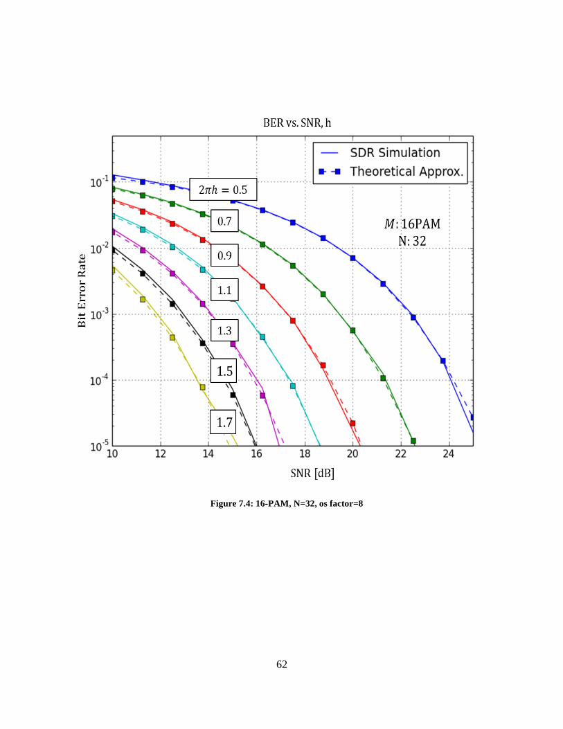
62
Figure 7.4: 16-PAM, N=32, os factor=8

63
Figure 7.5: 32-PAM, N=32, os factor=8
64
Figure 7.6: 64-PAM, N=32, os factor=8
65
The Figures 7.3 through 7.6 show that the GNU Radio CE-OFDM implementation performs very
close to the theoretical approximation, for SNR levels above the FM threshold ( > 10 dB). The
FM threshold effect can be observed more prominently in the lower modulation indices of the 32
and 64-PAM simulations, as the curves of the simulated data begin to deviate from the theoretical
approximation before the 10 dB threshold.
66
8 CONCLUSIONS
In this thesis, the CE-OFDM waveform was examined as a solution to the high peak-to-average-
power ratio (PAPR) problem of OFDM. CE-OFDM averts the necessity for highly linear, power-
inefficient amplification of OFDM by employing phase modulation to transform the high-PAPR
multicarrier signal into a constant envelope signal, like FSK or GMSK, which can be amplified
with non-linear power amplifiers at near saturation levels of efficiency.
The primary contribution of this thesis was a highly tunable software-defined radio (SDR)
implementation of the waveform which enables rapid-prototyping and testing of CE-OFDM
systems. A software ‘test bench’ was created to enable rapid configuration and testing of the CE-
OFDM waveform over all permutations of its parameters, over both simulated and physical RF
channels, and the results of a baseband simulation of the CE-OFDM receiver in an AWGN channel
validate the performance of the signal processing implementation. Thus, the SDR implementation
of this thesis proves to be viable framework for prototyping and testing CE-OFDM systems.
8.1 Further Research
The following subsections include recommendations for extending and applying the SDR
framework for further research.
8.1.1 Extending Waveform Implementation
Using the GNU Radio software framework a number of extensions can be readily added to the
current waveform implementation. The waveform can be extended to include blocks for
encoding/decoding, scrambling/de-scrambling, and equalization, to create a more sophisticated
communications system.
8.1.2 Extending Simulation and Analysis
The waveform simulation testbench can be extended to test error rate performance and spectral
efficiency of the waveform over a number of modulation parameters, coding rates and decoder
algorithms, equalization techniques, and multipath channel models to perform in-depth and
multivariate analysis of waveform performance.
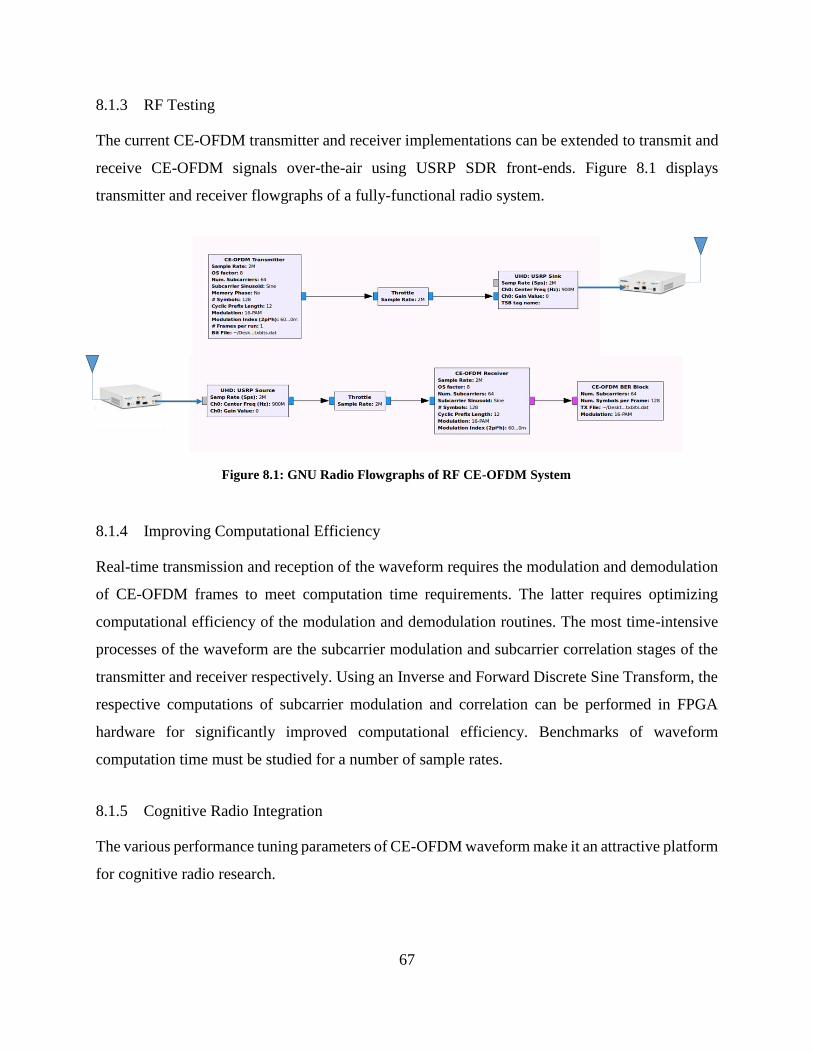
67
8.1.3 RF Testing
The current CE-OFDM transmitter and receiver implementations can be extended to transmit and
receive CE-OFDM signals over-the-air using USRP SDR front-ends. Figure 8.1 displays
transmitter and receiver flowgraphs of a fully-functional radio system.
8.1.4 Improving Computational Efficiency
Real-time transmission and reception of the waveform requires the modulation and demodulation
of CE-OFDM frames to meet computation time requirements. The latter requires optimizing
computational efficiency of the modulation and demodulation routines. The most time-intensive
processes of the waveform are the subcarrier modulation and subcarrier correlation stages of the
transmitter and receiver respectively. Using an Inverse and Forward Discrete Sine Transform, the
respective computations of subcarrier modulation and correlation can be performed in FPGA
hardware for significantly improved computational efficiency. Benchmarks of waveform
computation time must be studied for a number of sample rates.
8.1.5 Cognitive Radio Integration
The various performance tuning parameters of CE-OFDM waveform make it an attractive platform
for cognitive radio research.
Figure 8.1: GNU Radio Flowgraphs of RF CE-OFDM System
68
9 REFERENCES
[1] Ahmed, Ahsen, Steve Thompson, and James Zeidler. "Constant Envelope OFDM with
Channel Coding." Milcom 2006 (2006)
[2] Ahmed, Ahsen U., Steve C. Thompson, David W. Chi, and James R. Zeidler. "Subcarrier
Based Threshold Performance Enhancement in Constant Envelope OFDM." MILCOM
2012 - 2012 IEEE Military Communications Conference (2012).
[3] Bogucka, Hanna, and Andrea Conti. "Degrees of Freedom for Energy Savings in Practical
Adaptive Wireless Systems." IEEE Commun. Mag. IEEE Communications Magazine 49.6
(2011): 38-45.
[4] Carroll, Aaron, and Gernot Heiser. "An Analysis of Power Consumption in a Smartphone."
(n.d.).
[5] "Daughterboard Properties." USRP Hardware Driver and USRP Manual:
Daughterboards. N.p., n.d. Web. <http://files.ettus.com/manual/page_dboards.html>.
[6] Joung, Jingon, Chin Keong Ho, and Sumei Sun. "Spectral Efficiency and Energy
Efficiency of OFDM Systems: Impact of Power Amplifiers and Countermeasures." IEEE
J. Select. Areas Commun. IEEE Journal on Selected Areas in Communications 32.2 (2014):
208-20.
[7] Mestdagh, Dennis J. G, PhD. "Reduction Peak-to-Average-Power-Ratio of OFDM
Systems: A Tutorial Overview." Academia. N.p., Oct. 2014.
[8] Reed, Jeffrey Hugh. "Characteristics and Benefits of a Software Radio." Software Radio:
A Modern Approach to Radio Engineering. Upper Saddle River, NJ: Prentice Hall, 2002.
4.

69
[9] SBX-40 400 MHz. Ettus Research, n.d. Web.
<https://www.ettus.com/product/details/SBX>.
[10] Talbot, David. "Efficiency Breakthrough Promises Smartphones That Use Half the Power."
MIT Technology Review. N.p., 31 Oct. 2012.
[11] Thompson, S.c., A.u. Ahmedt, J.g. Proakis, and J.r. Zeidler. "Constant Envelope OFDM
Phase Modulation: Spectral Containment, Signal Space Properties and Performance."
IEEE MILCOM 2004. Military Communications Conference, 2004. (n.d.): n. pag. Web.
[12] Thompson, Steve, Ahsen Ahmed, John Proakis, James Zeidler, and Michael Geile.
"Constant Envelope OFDM." IEEE Transactions on Communications IEEE Trans.
Commun. 56.8 (2008): 1300-312.
[13] Thompson, Steve C. Constant Envelope OFDM Phase Modulation. Diss. U of California,
San Diego, 2005.
[14] "USRP2 and N2x0 Series Features List." USRP Hardware Driver and USRP Manual:
USRP2 and N2x0 Series. Ettus Research, n.d. Web.
<http://files.ettus.com/manual/page_usrp2.html>.
[15] Varahram, Pooria, Borhanuddin Mohd. Ali, and Somayeh Mohammady. "Power
Amplifiers in Wireless Communications." Power Efficiency in Broadband Wireless
Communications. N.p.: CRC, 2014. 23-59. Print.
[16] "What Is GNU Radio and Why Do I Want It?" WhatIsGR. N.p., n.d. Web.
<https://gnuradio.org/redmine/projects/gnuradio/wiki/WhatIsGR>.
[17] Yang, Samuel C. "Time Dimension: Multipath Delay Spread." OFDMA System Analysis
and Design. Boston: Artech House, 2010. 30.
70
[18] Robertson, Andrew, et al. A Constant Envelope OFDM Implementation on GNU Radio.
No. NRL/MR/5524--15-9575. Naval Research Lab Washington DC Networks and
Communication Systems Branch, 2015.
[19] "NI USRP-2920 Block Diagram." National Instruments. N.p., n.d. Web.
<http://zone.ni.com/reference/en-XX/help/373380B-01/usrphelp/2920_block_diagram/>.
[20] Rosu, Iulian. "RF Power Amplifiers." RF Technical Articles. YO3DAC - VA3IUL, n.d.
Web. <http://www.qsl.net/va3iul/>.
[21] Thompson, Steve, John Proakis, James Zeidler, and Michael Geile. "Constant Envelope
OFDM in Multipath Rayleigh Fading Channels."Milcom 2006 (2006): n. pag. Web.
[22] Ahmed, Ahsen U., Steve C. Thompson, and James R. Zeidler. "Threshold Extending
Receiver Structures for CE-OFDM." MILCOM 2007 - IEEE Military Communications
Conference (2007)


![1 Constant Envelope Signaling in MIMO Channels · arXiv:1605.03779v1 [cs.IT] 12 May 2016 1 Constant Envelope Signaling in MIMO Channels Borzoo Rassouli and Bruno Clerckx Abstract](https://img.dokumen.tips/doc/110x75/5f0322117e708231d407b393/1-constant-envelope-signaling-in-mimo-channels-arxiv160503779v1-csit-12-may.jpg)


![IMPLEMENTATION MODELS FOR ENERGY RECOVERY …pdfs.semanticscholar.org/92ea/1c76786204a9aede756fbb8680028d4f23bc.pdfbuilding envelope. New regulations [6, 7, 11] made compulsory for](https://img.dokumen.tips/doc/110x75/5fa209ccde57b01ffa6d4674/implementation-models-for-energy-recovery-pdfs-building-envelope-new-regulations.jpg)