Embed Size (px)
Citation preview

Rochester Institute of TechnologyRIT Scholar Works
Theses Thesis/Dissertation Collections
2009
Design and implementation of a computationalcluster for high performance design and modelingof integrated circuitsCharles J. Gruener
Follow this and additional works at: http://scholarworks.rit.edu/theses
This Thesis is brought to you for free and open access by the Thesis/Dissertation Collections at RIT Scholar Works. It has been accepted for inclusionin Theses by an authorized administrator of RIT Scholar Works. For more information, please contact [email protected].
Recommended CitationGruener, Charles J., "Design and implementation of a computational cluster for high performance design and modeling of integratedcircuits" (2009). Thesis. Rochester Institute of Technology. Accessed from

Design and Implementation of a Computational Cluster for
High Performance Design and Modeling of Integrated Circuits
by
Charles J. Gruener
A Thesis Submitted in Partial Fulfillment of the Requirements for the Degree of Master of Science in Microelectronic Engineering
Department of Microelectronic Engineering Kate Gleason College of Engineering
Rochester Institute of Technology Rochester, NY August 2009
Approved By:
_____________________________________________ ___________ ___
Dr. Santosh K. Kurinec Date Thesis Advisor
_ __ ___________________________________ _________ _____
Dr. Lynn F. Fuller Date Committee Member
_____________________________________________ ______________
Dr. Dhireesha Kudithipudi Date Committee Member

ii
Thesis Release Permission Form
Rochester Institute of Technology Kate Gleason College of Engineering
Title: Design and Implementation of a Computational Cluster for High
Performance Design and Modeling of Integrated Circuits
I, Charles J. Gruener, hereby grant permission to the Wallace Memorial Library of the
Rochester Institute of Technology to reproduce this document in whole or part that any
reproduction will not be for commercial use or profit.
_________________________________
Charles J. Gruener _________________________________
Date

iii
Dedication
To my wife,
Jennifer R. Gruener
for her endless love,
support and patience.

iv
Acknowledgements
I would like to thank my primary advisor, Dr. Santosh Kurinec, as well those on my
advisory committee: Dr. Lynn Fuller and Dr. Dhireesha Kudithipudi. It is because of
their optimism and dedication that this work has been a success.
To the RIT faculty and staff that I have had the pleasure to work with, I thank you for
your continued tutelage and constant support of my personal goals.
Additional thanks goes out to the countless students that I have been able to serve as a
System Administrator and Mask Making Engineer while employed at RIT. There is no
way I could list them all, but I’d like to at least acknowledge the few who directly helped
make this work possible: Christopher Murphy and Jordan Bean for giving me the
inspiration for this project and for helping me physically build the cluster, and Melissa
Dempsey for her patience in bringing me up to speed with Cadence and the use of her
design to prove this work as valid.

v
Abstract
Modern microelectronic engineering fabrication involves hundreds of processing
steps beginning with design, simulation and modeling. Tremendous data is acquired,
managed and processed. Bringing together Information Technology (IT) into a
functional system for microelectronic engineering is not a trivial task. Seamless
integration of hardware and software is necessary. For this purpose, knowledge of design
and fabrication of microelectronic devices and circuits is extremely important along with
knowledge of current IT systems.
This thesis will explain a design methodology for building and using a computer
cluster running software used in the production of microelectronic circuits. The cluster
will run a Linux operating system to support software from Silvaco and Cadence. It will
discuss the selection, installation, and verification of hardware and software based on
defined goals. The system will be tested via numerous methods to show proper
operation, focusing on TCAD software from Silvaco and custom IC design software from
Cadence.
To date, the system has been successfully tested and performs well. Since the
target applications are doing simulations that are independent of each other,
parallelization is very easy and user friendly. By simply adding more computers with
more CPUs, the maximum number of people and processes that can be supported scales
linearly. With a staged approach and the selection of the right software for the job, the
integration of IT components to build a computer cluster for microelectronic applications
can be completed successfully.

vi
Table of Contents
Thesis Release Permission Form.........................................................................................ii
Dedication.......................................................................................................................... iii
Acknowledgements.............................................................................................................iv
Abstract................................................................................................................................v
Table of Contents................................................................................................................vi
List of Figures.................................................................................................................. viii
List of Tables .....................................................................................................................xii
Glossary ........................................................................................................................... xiii
Chapter 1 Introduction......................................................................................................1
1.1. Background............................................................................................................1
1.2. Motivation .............................................................................................................7
1.3. Computer Clusters .................................................................................................8
1.4. Goals and Objectives ...........................................................................................13
Chapter 2 Operating System Selection ...........................................................................14
Chapter 3 Hardware Selection ........................................................................................17
Chapter 4 Software Selection .........................................................................................20
Chapter 5 Software Installation ......................................................................................23
5.1. Operating System ................................................................................................23
5.2. Sun Grid Engine ..................................................................................................36
5.3. Silvaco .................................................................................................................48
5.4. Cadence ...............................................................................................................56
Chapter 6 Results and Analysis ......................................................................................63

vii
6.1. Sun Grid Engine ..................................................................................................63
6.2. Silvaco .................................................................................................................65
6.3. Cadence ...............................................................................................................76
Chapter 7 Conclusions....................................................................................................86
Appendix A – Master Node Kickstart File ........................................................................88
Appendix B – Compute Node Kickstart File.....................................................................96
Appendix C – Sun Grid Engine Configuration File ........................................................104
Bibliography ....................................................................................................................109
viii
List of Figures
Figure 1 – Components of the Microelectronic Process......................................................1
Figure 2 - Digital IC Physical Design Flow ........................................................................3
Figure 3 - The Analog IC Design Process ...........................................................................4
Figure 4 - Fastest Clock Speed vs. Time for Intel Processors .............................................6
Figure 5 - Clock Speed of Introduced Intel Processor vs. Time..........................................7
Figure 6 - Cluster of Servers for High-Availability and Redundancy.................................9
Figure 7 - Computational Cluster for High Performance Computing ...............................10
Figure 8 - A General Diagram of the Computer Engineering Intel Cluster ......................12
Figure 9 - TCAD Overview...............................................................................................21
Figure 10 - Sample Minimal Kickstart Script....................................................................24
Figure 11 - Sample /etc/exports File..................................................................................27
Figure 12 - DHCP Server Sample /etc/dhcpd.conf File ....................................................29
Figure 13 - Name Server Sample /etc/named.conf File.....................................................31
Figure 14 - Name Server phoenix.domain File .................................................................32
Figure 15 - Name Server reverse.phoenix.domain File.....................................................32
Figure 16 - TFTP Server Sample /etc/xinetd.d/tftp File ....................................................33
Figure 17 - TFTP Server Sample PXE localboot File .......................................................33
Figure 18 - TFTP Server Sample PXE kickstart File ........................................................34
Figure 19 - Firewall Sample /etc/sysconfig/iptables File ..................................................35
Figure 20 - Sun Grid Engine Installation Wizard Welcome Screen..................................37
Figure 21 - Sun Grid Engine Component Selection ..........................................................38
Figure 22 - Sun Grid Engine Main Configuration.............................................................39

ix
Figure 23 - Sun Grid Engine Spooling Configuration.......................................................40
Figure 24 - Sun Grid Engine Host Selection .....................................................................41
Figure 25 - Create Links to the SGE Environment Scripts ...............................................41
Figure 26 - Sun Grid Engine Qmon Program....................................................................43
Figure 27 - Sun Grid Engine Administration Host Configuration ....................................44
Figure 28 - Sun Grid Engine Submit Host Configuration .................................................45
Figure 29 - Sun Grid Engine Host Groups Configuration.................................................46
Figure 30 - Sun Grid Engine Execution Host Configuration ............................................47
Figure 31 - Sun Grid Engine Interactive Parameters.........................................................48
Figure 32 - Sun Grid Engine qlogin_wrapper.sh...............................................................48
Figure 33 - Silvaco SFLM Installation Example...............................................................50
Figure 34 - Silvaco SFLM Web Management Interface Initial Screen .............................51
Figure 35 - Silvaco SFLM Register License Server Screen ..............................................52
Figure 36 - Silvaco SFLM Register Online Screen ...........................................................52
Figure 37 - Silvaco SFLM Home Screen ..........................................................................53
Figure 38 - Silvaco SFLM New License Selection Screen ...............................................54
Figure 39 - Contents of the /etc/profile.d/tools.sh Script...................................................54
Figure 40 - Contents of the /tools/env.d/silvaco.sh Script.................................................55
Figure 41 - Cadence InstallScape Home Menu .................................................................57
Figure 42 - Cadence InstallScape Releases Selection Window.........................................58
Figure 43 - Cadence InstallScape Wizard Release Selection Window .............................59
Figure 44 - Cadence InstallScape Directory Selection Window .......................................60
Figure 45 - Cadence InstallScape Product Selection Window ..........................................61

x
Figure 46 - Contents of the /tools/env.d/cadence.sh Script ...............................................62
Figure 47 - Sun Grid Engine Functional Diagram.............................................................65
Figure 48 - Silvaco VWF Splash Screen ...........................................................................66
Figure 49 - Silvaco VWF Open or Create an Experiment.................................................67
Figure 50 - Silvaco VWF Grid Preferences.......................................................................68
Figure 51 - Silvaco VWF Main Operation Window .........................................................69
Figure 52 - Silvaco VWF Preferences Window ................................................................70
Figure 53 - Silvaco VWF Import Deck Selection Window...............................................70
Figure 54 - Silvaco VWF Variables Defined in the Deck .................................................71
Figure 55 - Silvaco VWF Initial Tree Layout ...................................................................72
Figure 56 - Silvaco VWF Experiment Design Window....................................................73
Figure 57 - Silvaco VWF Final Tree Layout.....................................................................74
Figure 58 – Bottom Half of Shell Output of "watch qstat -f"............................................75
Figure 59 - Silvaco VWF Data Exported to Spayn ...........................................................76
Figure 60 - Cadence Virtuoso Splash Screen ....................................................................77
Figure 61 - Cadence Virtuoso Main Window....................................................................78
Figure 62 - Cadence Virtuoso Library Manager Window.................................................78
Figure 63 - Cadence Virtuoso Schematic Editor ...............................................................79
Figure 64 - Cadence Virtuoso Analog Design Environment Window..............................80
Figure 65 - Cadence Virtuoso Updated Analog Design Environment Window ...............80
Figure 66 - Cadence Virtuoso Simulator/Directory/Host Window ...................................81
Figure 67 - Cadence Virtuoso Analog Corners Analysis Window....................................82
Figure 68 - Differential Nonlinearity and Integral Nonlinearity of the DAC....................83

xi
Figure 69 - Cadence Virtuoso Analog Distributed Processing Window...........................84

xii
List of Tables
Table 1 - Processor Millions of Instructions per Second (MIPS)........................................8
Table 2 - System Specifications for the Computer Engineering Intel Cluster Nodes .......11
Table 3 - Silvaco Product Platforms..................................................................................14
Table 4 - Sun Grid Engine Component Definitions ..........................................................64

xiii
Glossary
Central Processing Unit (CPU) An electronic circuit that can execute computer
programs
Digital-to-Analog Converter (DAC) a device for converting a digital (usually
binary) code to an analog signal (current, voltage or electric charge)
Integrated Circuit (IC) A miniaturized electronic circuit consisting of
semiconductor devices and passive components that has been
manufactured in the surface of a thin substrate of semiconductor material
Information Technology (IT) The study, design, development, implementation,
support or management of computer-based information systems,
particularly software applications and computer hardware
Network File System (NFS) A file system protocol that allows a user on a client
computer to access files over a network in a manner similar to how local
storage is accessed
Operating System (OS) An interface between hardware and user; an OS is
responsible for the management and coordination of activities and the
sharing of the resources of the computer
Process Design Kit (PDK) A set of files used within the semiconductor industry to
model transistors for a certain technology for a certain foundry
Standard Floating License Manager (SFLM) The name of Silvaco Data Systems’
floating license manager
Sun Grid Engine (SGE) An open source batch-queuing system developed by Sun
Microsystems

xiv
Symmetric Multiprocessing (SMP) Two or more similar processors connected
via a high-bandwidth link and managed by one operating system, where
each processor has equal access to I/O devices
Technology Computer Aided Design (TCAD) a branch of electronic design
automation that models semiconductor fabrication and semiconductor
device operation. The modeling of the fabrication is termed Process
TCAD, while the modeling of the device operation is termed Device
TCAD.

1
Chapter 1 Introduction
1.1. Background
The microelectronic industry has a long established history of pushing the limits
of technology. It is because of this innovation and rapid development schedule that
numerous companies are profitable. It stands to reason that a long-standing model has
been established and reproduced over time. It is these areas that this work will
investigate and evaluate to see if they can be accelerated by a computational cluster.
Figure 1 – Components of the Microelectronic Process

2
The major components of the microelectronic process, Figure 11, include several
different domains of interest. Primarily, they stand on their own as individual areas of
the overall process. However, they do overlap with one another, as is quite often noticed
in microelectronic fabrication. Areas of feedback will provide modifications and insight
into other aspects of the design and simulation process. Circuit and chip design will rely
on the models that are developed from the processes used while certain processes will
need to be modified to do what the circuit demands.
All integrated circuit design can be broken down into two categories, digital and
analog. Mixed-signal design is simply working with both digital and analog signals
simultaneously. Digital IC design has clearly defined steps and procedures to produce
circuits. Analog IC design is less rigid, typically done in a non-hierarchical manner,
resulting in little use of repeated blocks.
The first subset of digital IC design is called electronic system level (ESL) design.
ESL design is the utilization of appropriate abstractions in order to increase
comprehension about a system, and to enhance the probability of a successful
implementation of functionality in a cost-effective manner2. It is the highest level of
abstraction when dealing with digital IC design. The basic idea is to model the entire
system operation in a high-level language such as C/C++, SystemC, or MATLAB. This
exercise can give the designer insight into the overall operation and functional blocks of
the system.
The next step in digital IC design is called register transfer level (RTL) design and
utilizes the functional blocks defined in the previous ESL design step. RTL design
defines a circuit's behavior in terms of the flow of signals (or transfer of data) between
3
hardware registers, and the logical operations performed on those signals. Hardware
description languages, such as Verilog and VHDL, create high-level representations of a
circuit, from which lower-level representations and ultimately actual wiring can be
derived. This step is ultimately responsible for the chip doing the right thing.
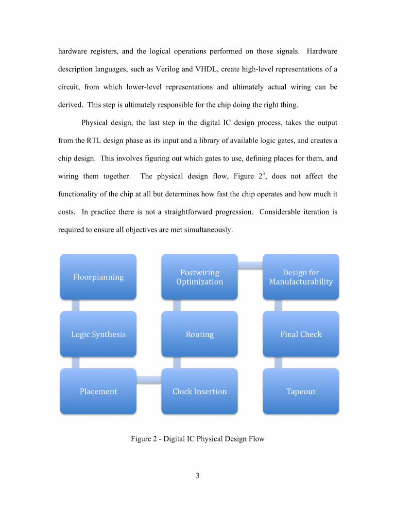
Physical design, the last step in the digital IC design process, takes the output
from the RTL design phase as its input and a library of available logic gates, and creates a
chip design. This involves figuring out which gates to use, defining places for them, and
wiring them together. The physical design flow, Figure 23, does not affect the
functionality of the chip at all but determines how fast the chip operates and how much it
costs. In practice there is not a straightforward progression. Considerable iteration is
required to ensure all objectives are met simultaneously.
Figure 2 - Digital IC Physical Design Flow

4
Analog IC design is much more difficult to define into a series of steps that are
rigidly followed. Analog IC design is performed at the circuit level and designs contain a
high amount of complexity. An analog design engineer needs to possess a strong
understanding of the principles, concepts and techniques involved in the electrical,
physical, and testing methodologies employed in circuit fabrication. Figure 31 gives an
overview of the design process utilized. As one can readily see, there is continuous
feedback from later steps in the process that help the designer in the early stages of the
electrical design.
Figure 3 - The Analog IC Design Process

5
All of this complexity in the IC design process relies heavily on the software and
hardware previously manufactured by the industry. The next generation of processors
and integrated circuits is only made possible by the previous generation. All of this
technology, software and hardware, encompasses a broader term known as Information
Technology (IT). The Information Technology Association of America defines IT as the
study, design, development, implementation, support or management of computer-based
information systems, particularly software applications and computer hardware4.
Basically, when computer and communications technologies are combined, the result is
information technology.
Information technology is an ever-expanding need of any organization.
Implemented properly, it has the potential to save your organization lots of time and
money. When done without a clear plan or design strategy, a lot of time can be wasted,
causing end-user frustration and decreased productivity. There are many pieces to the IT
puzzle that have countless interdependencies. While things have certainly gotten easier
over the years, it still takes a dedicated effort by many individuals to produce a working
solution.
Some of the basic components of IT include workstations, laptops, servers,
switches, routers, wireless access points, and many other components. All of these
components communicate with each other over physical or wireless networks.
Integrating all of these components into a functional system that is user-friendly is no
easy task.
The central processing unit (CPU) is the main component that drives the
performance of microelectronic software applications. The faster the CPU, the faster

6
results from a simulation can be obtained. Using the data that Intel publishes about its
processors5, we can see some interesting trends. Figure 4 plots the fastest available clock
speed of Intel’s processors over time from its first processor in 1971 to late 2005.
Sometime in 2000, a large increase in clock speed was experienced, translating to
increased performance from the CPUs.
Figure 4 - Fastest Clock Speed vs. Time for Intel Processors
Now taking a look at Figure 55, a plot of the clock speeds of Intel’s introduced
processors from 2006 until the end of 2008, something has started to happen. Clock
speed of the processors has started to stabilize. Something else must be contributing to
the increase in performance of processors in the past three years.
Besides architecture changes and device scaling improvements, the next
advancement in the area of the CPU is multiple cores. Intel first released a two-core

7
processor back in October of 2005 and it only took Intel just over a year to release a four-
core processor in November 2006. Since then, Intel has continued to ramp up the number
of products it produces with multiple cores. AMD was the first to release a two-core
processor but has since fallen behind Intel in the number of cores race. Roadmaps show
both manufacturers coming out with even more cores per processor in the future.
Figure 5 - Clock Speed of Introduced Intel Processor vs. Time
1.2. Motivation
Even with multiple cores, one computer has a limited amount of processing
power. It is sometimes desirable to find a solution to produce results faster than what one
computer can do. Although instructions per second (IPS) are continuing to increase over
time thanks to multiple processor cores5 (Table 1) and other architecture changes, this

8
alone will not be able to make the current serially processed jobs perform faster without
taking steps to modify our design practices.
Processor Speed Year Cores MIPS Intel Core 2 Extreme QX6700 2.66 GHz 2006 2 49,161 Intel Core 2 Extreme QX9770 3.2 GHz 2008 2 59,455 Intel Core i7 Extreme 965EE 3.2 GHz 2009 4 76,383
Table 1 - Processor Millions of Instructions per Second (MIPS)
The industry has made multiple processor systems commonplace. This means
that parallel processing is the way of the future and we need to figure out the best way to
utilize this hardware to increase the speed of the device simulations being performed. If
parallelization of the code is possible, one should not limit the workspace to that of just
one computer. A cluster of computers is the ideal environment to run massively parallel
computations, one that the microelectronic industry can readily utilize.
1.3. Computer Clusters
The term cluster can be used to define any number of groupings of computers and
is not limited to one type. There are many types of clusters, with the two most common
ones being high-availability and computational.
High-availability clusters have some sort of balancer that sits between the client
that connects to a service and the cluster of servers running the service the client wishes
to connect to. This configuration, as shown in Figure 6, is what powers most of the major
websites on the Internet. In order to handle the load from all of the computers requesting
information, the task needs to be split among many machines that are configured exactly
the same. A client attempts to connect and the balancer automatically establishes a
connection to one of the servers and lets that client and server communicate. The next
client connects and the balancer hands off that connection to another server and so on.

9
Figure 6 - Cluster of Servers for High-Availability and Redundancy
This layout allows for independence of action of the serving system behind the
balancer and gives the administrators of the systems flexibility for maintaining the
servers. Should one of the servers go down or not be acting properly, it can be removed
for the pool of machines without affecting the content being served to the clients as long
as the balancer is informed of the server’s removal. Typically, the balancer is also made
in such a way that there is some redundancy, thereby removing a single point of failure
for the entire system.
Computational clusters are machines that are connected together in such a way as
to gain a processing advantage over that of a single computer. In this scenario, as shown
in Figure 7, a client connects to a master, controlling computer. It is from this connection
that a job request is made that gets broken apart into many parallel tasks that run on the
compute nodes. Should the tasks need to communicate with one another, usually referred

10
to as inter process communication (IPC), a high speed message passing network separate
from the network used to connect the nodes make a significant difference in the rate at
which the cluster can complete its work. If the tasks running on the compute nodes are
independent of one another, this separate network is not needed, thereby saving costs and
complexity.
Figure 7 - Computational Cluster for High Performance Computing
With properly implemented IT infrastructure, processing and simulations of
devices for the microelectronic industry stand to be accelerated by a significant amount
when run on a clustered system. For the two cases that will be demonstrated, the
computational cluster for HPC is the ideal cluster layout. The Computer Engineering
Department owns an Intel based cluster that was used for this work. Table 2 shows some

11
of the specifications for the cluster nodes. Figure 8 gives a general diagram of the cluster
and how users interact with it.
Component Value Chasis Intel SR1530CL and SR1530CLR
Motherboard Intel S5000VCL
Processor 2 x Intel Xeon 5140 @ 2.33GHz Memory 2 x Kingston KVR667D2D8F5/1G
Hard Drive Maxtor 6L300S0 300GB Table 2 - System Specifications for the Computer Engineering Intel Cluster Nodes
Overall, each of the nodes has 4 physical processors (the Intel Xeon 5140 is a
dual-core processor,) 512MB of memory per core for a total of 2GB of memory per node,
and a 300GB hard drive for local storage of the operating system and temporary space.
There are 32 total machines, with one node dedicated to be the master node and the other
dedicated to be a storage node. This leaves 120 processors available in the remaining 30
compute nodes.
The storage node of the cluster has twice the amount of memory as each of the
master or compute nodes, 4GB, so it can speed up file-sharing operations by caching
them in memory. In addition, the storage node is connected to a Promise m500p RAID
array with 15 Seagate ST3320620AS 300GB drives. Configured, the storage system has
about 4TB of space available for use.

12
Figure 8 - A General Diagram of the Computer Engineering Intel Cluster
A cluster such as the one just described needs to have the proper environment to
work in. This means a dedicated room to handle the power the machines will consume,
cooling, and noise that the machines will produce. Data centers are the best place for
systems of this style. The design of a data center is a major factor in efficient cluster
operation but is outside the scope of this work.

13
1.4. Goals and Objectives
The main goal of this work is produce a methodology by which a cluster can be
built. Emphasis will be placed on the microelectronic industry software used in all
aspects of circuit, chip, and process design. At the end of this process, it should be the
system administrator’s job to make the system work without tedious intervention by the
end user. Simplicity in obtaining faster results should be paramount when considering
the environment, since most engineers will not be highly trained in the IT field.
The software applications that are used in the microelectronic industry are in
some way involved with the design and simulation of microelectronic circuits. More
often than not, a design of experiments is performed to determine a response based on
differing inputs. For example, modeling a diffusion process, one may wish to vary the
effects of implant dose, screening oxide thickness, drive-in temperature and drive-in time
to see the effects on the implanted dopant profile. The final dopant profile for a set of
initial conditions has no dependency on the other profiles that are obtained from different
initial conditions. These types of mass simulations that are all independent of one
another are the perfect candidates to be parallelized onto a compute cluster.
By increasing the number of simulations that can be done in the same amount of
time, the engineer will have control over how he wishes to proceed. By simply keeping
the simulations the same, the results will be produced that much faster. Another option
would be to increase the coverage of the experiment to produce greater insight into the
experiment. The engineer is then given more control over how best to utilize his time
and processing power to produce the results that best fit the individual situation instead of
being limited by time and processing power.

14
Chapter 2 Operating System Selection
The first task after purchasing a computer one needs to do when setting up a
cluster is to install an operating system (OS). Many considerations need to be made6 to
arrive at an answer as to which OS is the best for the environment. Certainly, it will help
to have a system administrator (or administrators depending on the size of the
deployment) that is familiar with the target OS. This will only help to alleviate any
problems that arise in a timely and efficient manor.
Obviously, the most important consideration is whether or not the target
application is supported under the operating system in question. Sometimes the
application is only supported under one operating system and the choice is then
unnecessary. But with more software manufacturers supporting more operating systems
now then ever, this situation doesn't arise as often anymore.
More often than not, when working with applications for the microelectronic
industry, the choice will be between Microsoft Windows and at least one Unix based OS.
Looking at the platform support from Silvaco7 is a fair example since it will be one of the
software vendors utilized in the final design. Table 3 shows what Silvaco lists as their
product platforms based on information they get from hardware and OS providers.
Operating System Vendor Operating System Version Sun Microsystems Sparc Solaris 9,10 (64-bit)
Microsoft Windows XP (32-bit), Vista Business Edition (32-bit or 64-bit)*
Linux Red Hat Enterprise 3, 4 or 5 (32-bit or 64-bit) * Our windows applications are 32-bit for compatibility with XP. When the applications
are run on Windows Vista 64-bit, they will be limited to about 3GB of memory. Table 3 - Silvaco Product Platforms

15
Using that information as a guideline, the next major consideration one should
make is the amount of memory that will be required. With prices of memory continuing
to fall8, it only makes sense to get as much memory for the system as will allow in your
budget. More of this will be covered in the next chapter, but for now lets assume your
application will have 4GB of RAM available to it. Looking at the options Silvaco
provides, the Microsoft Windows environment is the first one that will begin limiting
you, no matter if you choose to run the latest 64-bit OS they offer. This could potentially
become a major obstacle in the future, so planning for it now can alleviate any headaches
down the road.
That consideration alone will not make the decision for you, but for the purposes
of this work, let's take the case of Microsoft Windows not meeting your needs. This
means your choices have been narrowed to that of either Sun Solaris or Red Hat
Enterprise Linux. Sun Solaris has been around since 19929, and is an excellent choice for
symmetric multiprocessing as it supports a large number of CPUs. The downside, in this
case, is that the software vendor only provides binaries for the Sparc version of Solaris.
Many people still use Sparc and continue to purchase machines with that architecture;
however it is not mainstream hardware by any means. The majority of computer
hardware sold today is X86 compatible. Therefore, it looks like the vendor's supported
version of Linux, Red Hat Enterprise, will be what should be used.
Before settling on Red Hat Enterprise Linux, one more consideration should be
made. The Linux operating system that Red Hat makes is not free. In fact, all of the
operating systems that have been considered so far cost money. While numerous free
Linux operating systems exist, if you choose to use an unsupported OS, you can be left to

16
fend for yourself from the software vendor. Fortunately, a few operating system choices
are left. CentOS, which stands for Community Enterprise Operating System, and
Scientific Linux are two operating systems that are 100% binary compatible with Red
Hat Enterprise Linux and run all the software those vendors certify for Red Hat
Enterprise Linux.
Red Hat publishes the source code of their OS under the GNU General Public
License (GPL), specifically version 210. On the CentOS homepage, it states, "CentOS is
an Enterprise-class Linux Distribution derived from sources freely provided to the public
by a prominent North American Enterprise Linux vendor. CentOS conforms fully with
the upstream vendors redistribution policy and aims to be 100% binary compatible.
(CentOS mainly changes packages to remove upstream vendor branding and artwork.)
CentOS is free11." This almost always satisfies software vendors concerns regarding a
supported operating system. In those few instances that the vendor wants an actual copy
of Red Hat Enterprise Linux, it's safe to have one or two of these systems purchased and
setup to verify, saving a fair amount of money on the software needs of the cluster.
This exercise of determining operating system support needs to be repeated for all
of the software that is to be run on the cluster. The selection of this software will be left
for a later chapter, but for now it is important to realize that every situation is different
and only the end user can determine the final needs of the system after much deliberation.
Spending the time in the beginning stages of the project by collecting all of the
specifications from your software components will make the selection of your operating
system a much easier task.

17
Chapter 3 Hardware Selection
Over the years, a number of architectures have been developed and are in use in
the industry. Unless you are working on a project with very specific requirements that
contraindicate the use of X86 based systems, more likely than not, the final system will
be built based on that as the central architecture of your cluster. Parts are readily
available and cost per performance is only improving. Also, most processors on the
market today support 64-bit extensions to the X86 architecture. This is usually shortened
to X86-64 or even X64. The advantage of building your system up to support a 64-bit
computing environment is that it can handle more than 4GB of memory per process. This
is becoming a must for complex modern simulations.
There are numerous choices when it comes to purchasing hardware, which can be
a daunting task for those that aren’t familiar with the landscape. When building clusters,
to increase density of the systems, computers are typically rack mounted. This is one of
the best ways to increase the density of the systems and achieve the most power efficient
layout. System could also be purchased in blade configurations, but this is generally
done only for ultra high density. Something like this should be carefully investigated for
your deployment, as the added cost of blades may not be worth it when standard rack
mount systems may perform just as well.
A lot of headaches can be avoided by looking towards hardware compatibility
lists. More and more hardware vendors are starting to publish Linux compatibility lists,
thereby making this procedure much easier, though it is still not perfect. The best way to
proceed is look at the operating system documentation to see if it provides a list of
supported systems or vendors. For a first attempt, it may be best to go with a well-known

18
manufacturer’s computer instead of trying to build one from parts. In this work, the
cluster used is composed of Intel servers that were partially donated to the department.
The connections between all of the computers will need to be planned out as well.
The most common form of interconnect today is Ethernet. While there are certainly a lot
of other methods of connecting machines (token ring, Myrinet, InfiniBand) for a first
attempt at deployment, it would make the most sense to use what is most likely the
cheapest solution, gigabit Ethernet. Most rack mount systems come with two gigabit
Ethernet ports and generally provide enough bandwidth for the types of applications
being run in the microelectronic industry. Depending on the complexity of where the
cluster will be deployed, a simple unmanaged gigabit switch with enough ports for all
your machines will probably also provide the necessary connectivity. Should this not
work for any reason, be it bandwidth issues or latency issues, the investment you are
making into the equipment could serve as a backup network if another network
technology needs to be deployed later. Plus, relative to the total cost of the cluster, this
type of network is minimal in overall cost, typically less than 25% the cost of a single
node for a switch and all the connecting cables.
The final major consideration is the storage that is required for your cluster.
Again, there are numerous choices that can make the decision process seem difficult.
The growing popularity of network attached storage makes it an affordable choice, while
traditional methods of server based storage are sometimes more flexible. Hardware
vendor flexibility should always be a major consideration in any of these decisions,
especially in the storage arena. Purchasing something that it is difficult to get parts for in
the future can lead to downtime and frustration. It is for this reason that the storage

19
decision will come down to the available funds and desired access method. The cluster
used in this work has a dedicated storage node that uses the same hardware as the master
and execution nodes. It merely has additional storage attached to it via an add-in storage
controller and an external 15-drive storage chassis. This allows for easy migration should
any of the parts of the system become unavailable in the future.

20
Chapter 4 Software Selection
Once the operating system and physical components have been determined, the
finalized selection of software to run on the cluster can be completed. As demonstrated,
the selection of the operating system and the software go together. Software vendors will
only support certain configurations. It is with this information that the Linux operating
system was chosen as the operating system for the cluster.
Individual software packages that will run on the cluster will need to be evaluated
for system compatibility and vendor support. The example used in Chapter 2, Silvaco, is
from a vendor who produces a number of software packages. The one that is going to be
installed in this cluster environment is their TCAD package.
Figure 912 gives a hierarchy of process, device and circuit levels of the simulation
tools. The center boxes indicate the modeling level with each side containing icons that
depict the representative applications for TCAD. The left side, Extrinsic, focuses on
design for manufacturing issues: phase-shift masking, chemical-mechanical
planarization, and shallow-trench isolation. The right side, Intrinsic, shows the
traditional hierarchy of TCAD results and applications: process simulations, predictions
of drive current scaling, and extraction of technology files for the devices and parasitic
components.

21
Figure 9 - TCAD Overview
At the heart of microelectronic engineering, one needs to be able to produce a
device via some process, capture those steps into a concise computer model, and then run
simulations to improve upon the design. This is all part of the circular flow that provides
the necessary feedback to the device designers from what is actually being produced in
the fabrication facilities. Silvaco provides a software environment for running these
simulations. The flagship product that integrates all of the device simulators into a
cohesive design space is Virtual Wafer Fab (VWF). This will run the necessary design of
experiments on the TCAD models to better assist engineers determine the solutions to
their simulation needs.
With the process simulation handled by Silvaco VWF, circuit and chip
simulations can be handled by software from Cadence. While not an exhaustive list of all
the software that Cadence provides, the most important piece to be investigated will be
Cadence Virtuoso and its associated simulators. The Virtuoso Schematic Editor and
Analog Design Environment are part of the package known as Design Framework II from

22
Cadence. It is the product that is used for custom IC design and is one of the best analog
simulators in the market. There are numerous competing products to the ones just
mentioned and the selection of the right one for the environment will depend on many
factors. These two happen to be the ones that were already licensed and able to be
verified as operational with the cluster environment.
The last major consideration for software to be installed on the cluster is choosing
a job scheduler. Sometimes referred to as batch systems or distributed resource
managers, the job scheduler has many tasks to perform. Besides scheduling the
execution of jobs in queues that are controlled by priorities, the job scheduler needs to
provide interfaces to monitor these executions as well. Submission of the jobs to execute
should be automatic once requested.
Over time, numerous distributed resource management systems have been
developed. Once again, using the software manufacturer’s guidelines, the one common
product they seem to all moving towards supporting is Sun Grid Engine. Sun
Microsystems has made SGE since late 2000 and provides a free version of it along with
a paid, supported version. For our purposes, the free version will do everything we
require. This one software package will provide all of the necessary tools to provide
seamless cluster integration with the software packages from the vendors.

23
Chapter 5 Software Installation
Once all of the hardware and software selection process has been completed, the
last and probably most complex part of the process needs to be completed: installation
and configuration of the software. The reason that this is such a difficult thing to manage
is due to the volume of options the end user has when configuring the systems. Software
settings are also highly dependant upon the physical layout of the computer
configuration. This means that only the most structured of approaches and strict
adherence to software manufacturers' installation guidelines will lead to the most robust
of solutions. This, again, is going to be specific to each vendor that has been chosen in
the above process.
5.1. Operating System
The operating system in a Linux based distribution contains a kernel and the
necessary support applications to produce a functional environment. Each distribution
will have its own packages it deems necessary for a basic system, but the overall core
functionality and commands remain the same across the landscape.
Red Hat Enterprise Linux, and therefore CentOS, provides a number of methods
for installation that give the system administrator a number of powerful tools for rapid
system deployment. Besides the standard interactive installation that is achieved by
booting from an installation CD or DVD, one can also install over the network in an
automated fashion with a kickstart script. Figure 10 shows a sample minimal kickstart
file for a CentOS 5 system. Most of the commands are self-explanatory but some take a

24
bit more to understand. For now, the most important few to note are the ones that start
with a percent sign.
install url --url http://mirrors.rit.edu/centos/5/os/x86_64 lang en_US.UTF-8 keyboard us network --device eth0 --bootproto dhcp rootpw ChangeMe firewall --enabled --port=22:tcp selinux --enforcing timezone --utc America/New_York bootloader --location=mbr reboot clearpart --all --initlabel part /boot --fstype ext3 --size=128 part pv.01 --size=0 --grow volgroup vg0 pv.01 logvol swap --fstype swap --name=swap --vgname=vg0 \ --size=4096 logvol / --fstype ext3 --name=root --vgname=vg0 \ --size=1024 --grow %packages –nobase %post ( chvt 3 set -v yum -y update echo "root: [email protected]" >> /etc/aliases ) 2>&1 | tee /root/kickstart-post.log chvt 1
Figure 10 - Sample Minimal Kickstart Script
The first one encountered is %packages. This command specifies what packages
to include in your system. One would usually list package names one after another per
line to have them automatically installed. Since this is a minimal install, no packages are
listed and an extra option of nobase was added to keep the deployment as small as
possible. This is a good way to start working on a system if you want to decrease the

25
installed footprint to just include those packages that you are sure to use. It is always a
good idea from a security standpoint to install only those packages you need since any
software can be found to have vulnerabilities. By only installing what is absolutely
necessary, you reduce the risk of having a vulnerable package installed on the systems
you need to maintain.
The second option to take note of is %post. This is where a lot of power is given
to the system administrator. This section is fully customizable as it uses the Bourne shell
to interpret commands in this section. One can also pass the --interpreter option to the
%post command to choose the scripting language that is most familiar or more suited to
the environment. All of this information is documented in the Red Hat Enterprise Linux
Installation Guide13. Looking at the sample minimal kickstart file again, a few things
take place that need to be explained. All the output generated when the %post script is
run gets captured into a log file called kickstart-post.log located in /root. The command
“yum –y update” causes the system to perform an automatic update to ensure the latest
versions of packages are installed beyond what is delivered in the base system. This
ensures system compliance for any security and bug fixes. Lastly, any email generated
on the system for the root user will be forwarded to the email address [email protected]
and not stay on the system in a local mail store.
It is with this kickstart environment that systems can be rapidly deployed and
quickly reinstalled in the case of large configuration changes. A properly updated
kickstart file makes management of the nodes of a cluster much easier since you can be
sure that all nodes are exactly the same since they were all installed with the same
kickstart file. It takes a bit to get used to, but modern systems can be reinstalled in a

26
matter of minutes, making configuration file management less of an issue. Instead of
taking time to write scripts to make changes on the compute nodes, the updates are put in
the kickstart file and the machines are reinstalled.
This approach is exactly what is taken in the Rocks cluster distribution. Rocks
takes a lot of the management tasks of implementing a cluster and tries to make them
easier. From the about page of the Rocks web site: “Since May 2000, the Rocks group
has been addressing the difficulties of deploying manageable clusters. We have been
driven by one goal: make clusters easy. By easy we mean easy to deploy, manage,
upgrade and scale. We are driven by this goal to help deliver the computational power of
clusters to a wide range of scientific users. It is clear that making stable and manageable
parallel computing platforms available to a wide range of scientists will aid immensely in
improving the state of the art in parallel tools.14”
The Rocks cluster distribution utilizes either Red Hat Enterprise Linux or CentOS
as its base operating system and installs and configures an environment for you to aid in
rapid deployment of your cluster. It installs and configures DNS, DHCP, name services,
a kickstart environment, and a host of other settings that are selectable upon installation.
It makes a great first run at deploying a cluster but usually ends up installing a number of
extra packages that aren’t required, thereby leading to security concerns. Some of the
work done in this thesis was performed on a cluster running version 4.3 of the Rocks
cluster distribution. In the end, a custom cluster was built that used some of the
information obtained from the way Rocks installs machines to create a streamlined
kickstart script that has been tailored exclusively for an environment where
microelectronic applications will be used.

27
The storage node will be the first to be installed, as it is actually the easiest to get
up and running quickly. Figure 10 was an example minimal configuration file and can be
used to get your storage node installed quickly. After installation has completed, one
simply needs to format the storage area that is to be exported to all of the nodes. The
exported volumes are then configured in the file /etc/exports and has a format similar to
what is shown in Figure 11. The first column is the area of the file system to be exported
and the second column denotes to which machine and what permissions each of those
machines have. In this case, we are utilizing a trusted internal network and want any
machine that is deployed or will be deployed in the future to have access to the file
systems being exported. Therefore, instead of putting individual hostnames in the second
column, a network was defined, 10.0.0.0/255.0.0.0, and given access. Note that the
no_root_squash option means that the root user on the clients will have the same
privileges as the root user on the storage node when accessing the files. You may need to
adjust this for your environment as your security needs require.
/export/nfs-home \ 10.0.0.0/255.0.0.0(rw,no_root_squash,no_subtree_check) /export/nfs-tools 10.0.0.0/255.0.0.0(ro,no_subtree_check) /export/nfs-kickstart \ 10.0.0.0/255.0.0.0(rw,no_root_squash,no_subtree_check)
Figure 11 - Sample /etc/exports File
Once the /etc/exports file has been setup, as long as your storage node is on a
trusted network, you can make sure the firewall is disabled by first stopping it with the
command “service iptables stop” and the disabling the service with “chkconfig iptables
off”. Lastly, make sure the nfs service and the portmap service both start on system boot
with the commands “chkconfig nfs on” and “chkconfig portmap on”, respectively.
28
Restart the system to verify everything starts as expected and your storage node should be
serving the data the cluster needs.
The master node is the next to be installed and is the most complex of the nodes
to be installed. The kickstart file located in Appendix A gives a good feel for the amount
of customization that is required to produce a stable and full-featured working
environment for your users. The system has been designed to accept client connections
via SSH and has both an external, untrusted network interface and an internal, trusted
network interface.
Besides what is shown in the kickstart file for the master node, multiple other
services need to be configured. What follows is a configuration of the most important of
these services. The configuration of a name service, such as NIS or LDAP, is outside the
scope of this work and is usually already provided at some level in your environment.
Recommended for a new installation is a combination of LDAP and Kerberos for a new
deployment when possible.
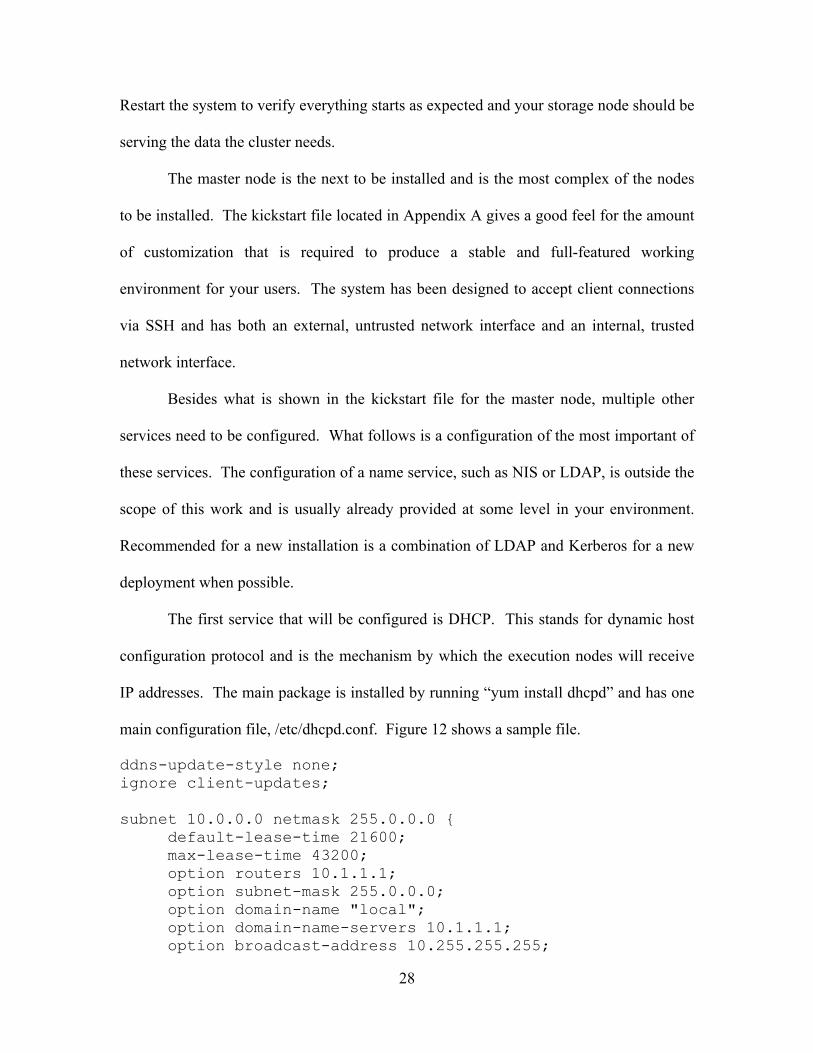
The first service that will be configured is DHCP. This stands for dynamic host
configuration protocol and is the mechanism by which the execution nodes will receive
IP addresses. The main package is installed by running “yum install dhcpd” and has one
main configuration file, /etc/dhcpd.conf. Figure 12 shows a sample file.
ddns-update-style none; ignore client-updates; subnet 10.0.0.0 netmask 255.0.0.0 {
default-lease-time 21600; max-lease-time 43200; option routers 10.1.1.1; option subnet-mask 255.0.0.0; option domain-name "local"; option domain-name-servers 10.1.1.1; option broadcast-address 10.255.255.255;

29
if (substring (option vendor-class-identifier, 0, 20) = "PXEClient:Arch:00002") {
# ia64 filename "elilo.efi"; next-server 10.1.1.1;
} elsif ((substring (option vendor-class-identifier, 0, 9) = "PXEClient") or
(substring (option vendor-class-identifier, 0, 9) = "Etherboot")) {
# i386 and x86_64 filename "pxelinux.0"; next-server 10.1.1.1;
} else { filename "pxelinux.0"; next-server 10.1.1.1;
} host phoenix.local {
hardware ethernet 00:15:17:00:8d:00; option host-name "phoenix"; fixed-address 10.1.1.1;
}
Figure 12 - DHCP Server Sample /etc/dhcpd.conf File
The first section of the file defines the subnet that is going to be used. In this
case, a full class A subnet was used, 10.0.0.0. The master node, phoenix.local, is also
listed as the domain name server and the PXE boot server. Lastly, an entry for the host
phoenix is included for completeness and also as an example for the other hosts that
should be entered into the configuration. By simply copying this one entry and
modifying it for each execute node that is needed, the DHCP server configuration file can
be completed quickly, requiring a “service dhcpd restart” when completed.
To find these hosts automatically via a name lookup instead of by IP address only
requires that a DNS server be installed on the master node as well. This can be
accomplished via numerous ways, but the easiest is to install just the main name server
called BIND. The command to type is “yum install bind caching-nameserver” so that

30
both BIND gets installed and so does the necessary configuration files for a caching name
server. The configuration files for BIND are stored in /etc and in /var/named. The first is
/etc/named.conf and can be seen in Figure 13.
options { directory "/var/named"; dump-file "data/cache_dump.db"; statistics-file "data/named_stats.txt"; memstatistics-file "data/named_mem_stats.txt"; forwarders { 129.21.3.17;129.21.4.18; }; }; controls { inet 127.0.0.1 allow { localhost; } keys { rndckey; }; }; zone "." IN { type hint; file "named.ca"; }; zone "localdomain" IN { type master; file "localdomain.zone"; allow-update { none; }; }; zone "0.0.127.in-addr.arpa" IN { type master; file "named.local"; allow-update { none; }; }; zone "0.0.0.0.0.0.0.0.0.0.0.0.0.0.0.0.0.0.0.0.0.0.0.0.0.0.0.0.0.0.0.ip6.arpa" IN { type master; file "named.ip6.local"; allow-update { none; }; }; zone "255.in-addr.arpa" IN { type master;

31
file "named.broadcast"; allow-update { none; }; }; zone "0.in-addr.arpa" IN { type master; file "named.zero"; allow-update { none; }; }; zone "local" { type master; notify no; file "phoenix.domain"; }; zone "10.in-addr.arpa" { type master; notify no; file "reverse.phoenix.domain"; }; include "/etc/rndc.key";
Figure 13 - Name Server Sample /etc/named.conf File
The most important things to configure in the /etc/named.conf file are the
forwarders, which handle DNS requests that the local server knows nothing about, and
last to defined zones. The domain name local was chosen for the environment since it
doesn’t clash with anything else that could be defined on an upstream DNS server. The
two files used for the local domain are phoenix.domain and reverse.phoenix.domain for
the forward and reverse DNS lookups, respectively. Figure 14 and Figure 15 show the
contents of these two files that are located in /var/named.
$TTL 3D @ IN SOA ns.local. root.ns.local. ( 1247078120 ; Serial 8H ; Refresh 2H ; Retry 4W ; Expire 1D ) ; Min TTL

32
; NS ns.local. MX 10 mail.local. localhost A 127.0.0.1 ns A 127.0.0.1 phoenix A 10.1.1.1
Figure 14 - Name Server phoenix.domain File
$TTL 3D @ IN SOA ns.local. root.ns.local. ( 1247078120 ; Serial 8H ; Refresh 2H ; Retry 4W ; Expire 1D ) ; Min TTL ; NS ns.local. MX 10 mail.local. 1.1.1 PTR phoenix.local.
Figure 15 - Name Server reverse.phoenix.domain File
The only things that need to be adjusted are the last lines in each of the file and
the serial number each time a change is made. Nodes are given what are known as A
records just like was done for the master node, phoenix. The DNS service can be then be
reloaded after making the changes with a “service named reload” command.
To support the network boot environment, a trivial file transfer protocol (TFTP)
server is needed. The command to install the TFTP server is “yum install tftp-server”
and should proceed with installing a package called xinetd as a dependency. Create a
directory in the newly installed directory /tftpboot called pxelinux. Edit the file
/etc/xinetd.d/tftp and make it have the contents shown in Figure 16.
service tftp { disable = no

33
socket_type = dgram protocol = udp wait = yes user = root server = /usr/sbin/in.tftpd server_args = -s /tftpboot/pxelinux per_source = 11 cps = 100 2 flags = IPv4 only_from = 10.0.0.0/8 }
Figure 16 - TFTP Server Sample /etc/xinetd.d/tftp File
The folder /tftpboot/pxelinux needs to contain the necessary files for booting a
machine from the network. First, it will need two files that are available from the web,
vmlinuz and initrd.img. The URL http://mirrors.rit.edu/centos/5/os/x86_64/isolinux is an
example of a place where the files can be obtained. Next, it requires the file pxelinux.0,
which should already be located on your system in /usr/lib/syslinux. Copy it from there.
Lastly, a folder pxelinux.cfg needs to be created with two files, one called localboot and
one called kickstart. The localboot file, shown in Figure 17, defines that a machine
should boot from the local hard drive and not boot from the network. The kickstart file,
shown in Figure 18, defines that a machine should boot from the network and attempt in
install itself via kickstart from the file specified on the append line. All that remains is to
enable the TFTP by enabling the xinetd service. The commands “chkconfig xinetd on”
and “service xinetd start” should be all that is necessary to finish the network boot
environment setup.
default linux prompt 0 label linux localboot 0
Figure 17 - TFTP Server Sample PXE localboot File

34
default kickstart prompt 0 label kickstart kernel vmlinuz append initrd=initrd.img \ ks=nfs:nfs-01.local:/export/nfs-kickstart/node.cfg \ ksdevice=eth0
Figure 18 - TFTP Server Sample PXE kickstart File
The only other configuration change needed on the master node is to make sure
the firewall is properly set for traffic. Linux uses the iptables framework to manage the
firewall for the system. Because the head node is acting as a router for the internal
network, the first thing that needs to be done is to turn on IP forwarding. This is done by
simply changing the file /etc/sysctl.conf. Find the line “net.ipv4.ip_forward = 0” and
change the 0 to a 1. If you don’t want to reboot the system, you can issue the command
“sysctl net.ipv4.ip_forward=1” to enable it immediately.
The file that controls the actions of the firewall is /etc/sysconfig/iptables. The
contents of the file listed in Figure 19 show a proper configuration for the cluster with a
couple of extras. The first section sets up the network address translation tables and
configures post routing to do IP masquerading. Lastly, the filter section allows all traffic
on the internal and loopback interfaces and only allows SSH and printer access from the
outside network.
*nat :PREROUTING ACCEPT [0:0] :POSTROUTING ACCEPT [0:0] :OUTPUT ACCEPT [0:0] -A POSTROUTING -o eth0 -j MASQUERADE COMMIT *filter :INPUT ACCEPT [0:0] :FORWARD ACCEPT [0:0] :OUTPUT ACCEPT [0:0] :RH-Firewall-1-INPUT - [0:0]

35
-A INPUT -j RH-Firewall-1-INPUT -A FORWARD -j RH-Firewall-1-INPUT -A FORWARD -i eth0 -o eth1 -m state --state RELATED,ESTABLISHED -j ACCEPT -A FORWARD -i eth1 -o eth0 -j ACCEPT -A RH-Firewall-1-INPUT -i lo -j ACCEPT -A RH-Firewall-1-INPUT -i eth1 -j ACCEPT -A RH-Firewall-1-INPUT -p icmp -m icmp --icmp-type any -j ACCEPT -A RH-Firewall-1-INPUT -p esp -j ACCEPT -A RH-Firewall-1-INPUT -p ah -j ACCEPT -A RH-Firewall-1-INPUT -d 224.0.0.251 -p udp -m udp --dport 5353 -j ACCEPT -A RH-Firewall-1-INPUT -p udp -m udp --dport 631 -j ACCEPT -A RH-Firewall-1-INPUT -p tcp -m tcp --dport 631 -j ACCEPT -A RH-Firewall-1-INPUT -m state --state RELATED,ESTABLISHED -j ACCEPT -A RH-Firewall-1-INPUT -p tcp -m state --state NEW -m tcp --dport 22 -j ACCEPT -A RH-Firewall-1-INPUT -j REJECT --reject-with icmp-host-prohibited COMMIT
Figure 19 - Firewall Sample /etc/sysconfig/iptables File
Now that the PXE environment exists on the master node, installation of the
execution nodes becomes trivial once the kickstart file has been created. See Appendix B
for a sample kickstart file that has been used in this environment. In addition, so SSH
keys get properly restored and other files are restored after a reinstall, the space being
exported on the storage node called /export/nfs-kickstart is utilized to hold these
important files.
The procedure to install an execution node is as follows. First figure out how to
configure the system to boot off of the network, as this is dependant on the hardware
obtained. Next, obtain the MAC address of the network card and enter that into the
master node’s DHCP and DNS servers’ configuration files. Restart the DHCP server
with the command “service dhcpd restart” and then reload the DNS server with the

36
command “service named reload”. Finally, boot the execute node and it should begin
installing over the network. A properly configured execute node should be available in
about 20-30 minutes based on the configuration file you use and the network bandwidth
available.
5.2. Sun Grid Engine
The open source version of Sun Grid Engine is found on the Sun Source website,
http://gridengine.sunsource.net/. From here you can download the binaries for the
platform you are installing, in this case Linux. Since the platform we are on supports a
64-bit environment, the binary obtained is the one for 64-bit Linux. As of this writing,
the version available is Grid Engine 6.2 Update 3, and the file is called ge62u3_lx24-
amd64.tar.gz. All instructions that are found here were adapted from the Sun
Microsystems Wiki, Sun Grid Engine 6.2u315.
A user account that acts as the SGE admin account needs to be created that will be
the same on all nodes of the cluster. This account can be created on each of the nodes
manually or stored in a central name service. This will depend on how you chose to
configure your name service during the installation of the operating system. Next, the
directory where SGE is to be installed should be shared to all of the nodes over NFS.
This location was chosen to be the “sge” user’s home directory since all of the home
directories are already being shared over NFS.
After downloading the ge62u3_lx24-amd64.tar.gz file from Sun’s web site,
become the user root. In a terminal on the master, type the command “tar -C
/home/sge/6.2u3 -xzf ge62u3_lx24-amd64.tar.gz --strip-components=1” to extract the
files from the archive. Two archives, ge-6.2u3-bin-lx24-amd64.tar.gz and ge-6.2u3-

37
common.tar.gz, will be created inside the folder /home/sge/6.2u3. Change into the folder
6.2u3 and type “for file in *; do tar -xzf $file; done” to extract the files from these two
archives. The installer is now ready to be invoked by running “./start_gui_installer” from
the terminal. A window should now be visible presenting the Sun Grid Engine installer.
Figure 20 - Sun Grid Engine Installation Wizard Welcome Screen
Click next to be presented with the Licensing Agreements. You must accept in
order to continue. After that you’ll be presented with a window asking you which
components you wish to install. This is the master node that is being installed so the only
component we wish to have installed is the Qmaster. Be sure to select a “Custom
installation” as well since we will be modifying some of the default installation

38
parameters to better suit our environment. The window should look like what is shown in
Figure 21 before proceeding.
Figure 21 - Sun Grid Engine Component Selection
After clicking next, you’ll be presented with a window asking you for the main
configuration parameters. Change the admin user to be the user sge that was created
earlier. The qmaster host is the host name of the master. Leave the cell name set to
default. The cluster name should be changed to something meaningful. Leave all the
other settings as default except for the administrator mail. Put in an email address that
you wish to have administrative email sent to. All other options are set as shown in
Figure 22. Be sure to uncheck the option to use JMX, as it is not needed in this
configuration.

39
Figure 22 - Sun Grid Engine Main Configuration
The next window is for configuring your spooling options. The defaults don’t
give you the flexibility to upgrade your version of SGE in the future. Therefore, you
should move your spool directories out of the version specific directory that is wants you
to put it in. In addition, the first cluster you create won’t be so large that you need to use
a fancy spooling method. It is easier to just use classic for now. Figure 23 has the
suggested final spooling configuration.

40
Figure 23 - Sun Grid Engine Spooling Configuration
The last thing needed before installing SGE is what hosts are going to be
configured along with the master. It is easy to add hosts with a few simple commands
after doing an initial installation, so we’ll leave just the master on the list shown in Figure
24 for now. Click install to begin installing the software. Make sure the software
installation reports success before proceeding to the next step.

41
Figure 24 - Sun Grid Engine Host Selection
The software should now be successfully installed. The installation script should
have automatically started the sge_qmaster binary. This binary is responsible for many
tasks that will be explained later. For now, just check to make sure it is running by
running “pgrep sge_qmaster” to get the process id of the running sge_qmaster process.
As long as the previous command returns some number, the daemon is running. Lastly,
add the settings to the default environment for logging in by creating links to the settings
files in the /etc/profile.d directory as shown in Figure 25.
ln –s /home/sge/6.2u3/default/common/settings.sh \ /etc/profile.d/sge.sh ln –s /home/sge/6.2u3/default/common/settings.csh \ /etc/profile.d/sge.csh
Figure 25 - Create Links to the SGE Environment Scripts

42
Adding an execution host is very straightforward and is handled via the command
line. First, the host needs to be added to those that are listed as administrative hosts.
This is accomplished by running “qconf –ah node-01” on the master. Better may be to
add all the nodes as administrative hosts now so they can be installed automatically later.
This simple bash script should do what you want: “for i in `seq –w 1 30`; do qconf –ah
node-$i; done”. Next, after logging in to the node, you have to source the start up script
for SGE. This is done with the command “source
/home/sge/6.2u3/default/common/settings.sh” and should be added to the default
environment, just as was done on the master node in Figure 25. Change to the directory
/home/sge/6.2u3 and run the following command, “./install_execd –noremote –auto
util/install_modules/sge_configuration.conf” after creating the sge_configuration.conf
file with the contents shown in Appendix D. Verify installation by running “qhost” and
see that the compute node is listed among the output.
Now that the node is installed, it is beneficial to set the environment such that
proper balancing of interactive jobs is done too. For this to happen, a couple of settings
need to be modified. We can modify the earlier bash script we used to make all of the
nodes administration hosts to also make them submit hosts. It will look like this: “for i
in `seq –w 1 30`; do qconf –as node-$i; done”. The easiest way to make the other
changes is to run the program “qmon” on the master node. This starts the graphical
interface shown in Figure 26.

43
Figure 26 - Sun Grid Engine Qmon Program
The program “qmon” is where all of the Sun Grid Engine parameters can be
modified after installation. While very powerful, it is only necessary to modify a small
section of configuration to get interactive jobs to work properly. You start off by clicking
on the fifth button on the top row, host configuration. Double check that all of your hosts
are listed in the four tabs, administration host, submit host, host groups, and execution
host. See Figure 27 through Figure 30 for how the host configuration tabs should look,
with one exception. Because sixteen of the computers were already installed and being
used in a Rocks cluster, there were not enough nodes to make all thirty available at the
time this paper was written. It should be obvious what changes need to be made to this
screen to obtain the desired results. Future results in this work will only show fourteen
nodes for this same reason.

44
Figure 27 - Sun Grid Engine Administration Host Configuration

45
Figure 28 - Sun Grid Engine Submit Host Configuration

46
Figure 29 - Sun Grid Engine Host Groups Configuration

47
Figure 30 - Sun Grid Engine Execution Host Configuration

48
Now that the settings have been verified, you can click done and return to the
main interface. Now click the sixth button on the top row, cluster configuration. Click
the host called “global” and then click the modify button. Click the advanced settings tab
and change the interactive parameters to be what is shown in Figure 31. Figure 32 has
the contents of the qlogin_wrapper.sh script that you’ll need to create16.
Figure 31 - Sun Grid Engine Interactive Parameters
#!/bin/sh HOST=$1 PORT=$2 /usr/bin/ssh -X -p $PORT $HOST
Figure 32 - Sun Grid Engine qlogin_wrapper.sh
5.3. Silvaco
Silvaco makes a number of software products that can be licensed via multiple
different methods. The instructions that follow will be based on the method that RIT has
entered into an agreement with Silvaco. This licensing method is known as a Silvco
OMNI license.
There are three separate packages that will need to be downloaded from Silvaco’s
website, http://www.silvaco.com/, to completely set up the working environment. Two
packages, TCAD and Virtual Wafer Fab (VWF), will be installed on the systems to a
location that is once again shared to all the nodes over NFS. The last package is the

49
standard floating licensing manager (SFLM), which should be installed on a dedicated
licensing machine for reliability.
The installation process is relatively easy and requires just a few simple
commands to be entered17. First, create a directory that will be accessible to all the nodes
in the NFS shared space. After downloading the latest TCAD release package, 07426-
tcad-2008-09-rh64.tar.gz as of this writing, extract it directly to this shared directory,
/tools/silvaco in our case, with the following command: “tar –C /tools/silvaco –xzf
07426-tcad-2008-09-rh64.tar.gz”. Repeat this process for the VWF release package,
09542-vwf-2008-09-rh64.tar.gz as of this writing, by extracting it to the exact same
directory, /tools/silvaco. That is all for now as the environment that will be set up will
depend on the license manager configuration.
Licensing of the Silvaco software is handled via Silvaco’s own licensing manager,
SFLM. This package is obtained as a download from Silvaco’s website just like the other
packages. This should be downloaded onto a dedicated machine and does not have to be
installed into a location that is accessible via NFS. Create a folder in a location suitable
for your environment, /opt/silvaco for example, and extract the files to that location with
the following command: “tar –C /opt/silvaco –xzf 09220-sflm-2008-09.tar.gz”.
To better manage the license server from the command line in the future, create a
file with the following command: “echo ‘export PATH=${PATH}:/opt/silvaco/bin’ >
/etc/profile.d/silvaco.sh”. Make this file executable by typing, “chmod a+x
/etc/profile.d/silvaco.sh”. This will put the Silvaco binaries into the default PATH for all
users who login to the license server. Logout and login again. Make sure the settings are
correct by trying to run “sflm –install” to start the license manager installation process.

50
After setting an administrative password for the SFLM interface, the installer should
complete. See Figure 33 for an example output of the installation process.
[root@silvachole ~]# sflm -install Version of rpc.sflmserverd : 8.0.12.R Version of sflm_monitord : 7.4.15.R Setting SFLM administrative password. New Password ? Running s_install version: 1.8.2.R please wait... Terminating SFLM RPC servers ... done. Running s_install version: 1.8.2.R please wait... Currently 5732612 KB free in /tmp (>= 8000) Preparing to install the SFLM server daemon. This procedure will modify or create the following system files: /etc/rc.d/init.d/sflm Backups will be created in /var/tmp/s_install.bak before any files are modified. Run '/opt/silvaco/etc/s_install -rm-bak' or '/var/tmp/s_install.bak/remove' to remove backup files. Do you wish to proceed? [y|n] y Verifying permissions ... done. Installing servers in init.d ... Installation done. Starting and verifying servers ... SFLM using license file: /var/opt/sflm/licenses SFLM server ready. Verification done. SFLM installation completed successfully. [root@silvachole ~]#
Figure 33 - Silvaco SFLM Installation Example
The next step is to open web browser with the following address,
http://<servername>:3162/. Figure 34 shows the web page that should appear to continue

51
the setup. Should it not appear, check your firewall settings on the license server to make
sure port 3162 is open.
Figure 34 - Silvaco SFLM Web Management Interface Initial Screen
Enter the password you just set to login to the web interface. You will now be
prompted with the screen shown in Figure 35. You need to register the license server
with Silvaco before a license file can be issued to you. If the machine is connected to the
Internet, the easiest way to proceed is to click the “Register Online” button. This is what
is the case in this example. After clicking that button, Figure 36 shows the screen that is
presented next. Fill out the information asked of you and click next to proceed. You
should receive a message stating, “Your details have been recorded, click next to activate
your server.” Click next.

52
Figure 35 - Silvaco SFLM Register License Server Screen
Figure 36 - Silvaco SFLM Register Online Screen
After receiving a screen stating you have successfully registered and activated
SFLM, you can add the subsequent license file you will receive from Silvaco. This is

53
handled via the admin interface on the SFLM web page. After clicking OK on the
registration complete page, click on the “Install New License(s)” button on the right side
of the page shown in Figure 37.
Figure 37 - Silvaco SFLM Home Screen
Most likely, the license file will be sent to you as an attachment via email. Save
the attached file from the email to a location on your computer. From the screen shown
in Figure 38, click the “Install Saved File” button. You’ll then be presented with a screen
that will request a license file location. Click “Browse” and select the downloaded
license file. As long as you receive a message stating SFLM has installed the license file,
you can now click “Done” and proceed with the rest of the installation procedure.

54
Figure 38 - Silvaco SFLM New License Selection Screen
As was the case with Sun Grid Engine, the Silvaco binaries need to be added to
the default PATH on the system. This will make it so users won’t have to type the full
path to the binary to run the program. One easy way to do this on systems that are
running numerous binaries off of an NFS mounted file system is to create a file called
“tools.sh” in the /etc/profile.d folder with the contents shown in Figure 39. Make sure the
file is executable and then place all the startup environment variables in their own files in
the NFS shared directory /tools/env.d, making sure the filename ends in .sh.
if ! [ `/usr/bin/id -u` = 0 ] ; then for i in /tools/env.d/*.sh ; do if [ -r "$i" ] ; then . $i fi done unset i fi
Figure 39 - Contents of the /etc/profile.d/tools.sh Script

55
Now, simply create an executable file called /tools/env.d/silvaco.sh with the
contents shown in Figure 40. The first export line sets the license server location, while
the second states that an OMNI license should be requested. The rest set the PATH and
LD_LIBRARY_PATH to include the necessary information as shown, ensuring it
doesn’t get set twice in the case of re-sourcing of these scripts when already having the
environment loaded.
export SFLM_SERVERS="silvachole.ce.rit.edu" export SFLM_OMNI=1 if ! echo $PATH | /bin/egrep -q "(^|:)/tools/silvaco/bin($|:)" ; then export PATH=${PATH}:/tools/silvaco/bin fi if ! echo $LD_LIBRARY_PATH | /bin/egrep -q "(^|:)/tools/silvaco/lib/mesa/6.2.1.R/x86_64-linux($|:)" ; then if [ -n "$LD_LIBRARY_PATH" ] ; then export LD_LIBRARY_PATH=${LD_LIBRARY_PATH}:/tools/silvaco/lib/mesa/6.2.1.R/x86_64-linux else export LD_LIBRARY_PATH=/tools/silvaco/lib/mesa/6.2.1.R/x86_64-linux fi fi
Figure 40 - Contents of the /tools/env.d/silvaco.sh Script
It should be noted that these settings only work for users using the bash shell,
which is perfectly fine in this environment. Should users require a different shell, a script
would need to be written in that language or the system should be setup to use something
like the package environment-modules found on the web at
http://modules.sourceforge.net/.

56
5.4. Cadence
Cadence makes a large number of software packages that are installed via
numerous methods. For this work, Cadence’s InstallScape software is the method by
which the software will be obtained and installed. Configuration after installation is still
a manual process left to the system administrator. Users still have the ability to
customize this environment even further to support the individual needs of the many
diverse projects they simulate. Lastly, Cadence’s license server will also need to be
downloaded and configured to support the licensing of the software environment.
Cadence calls the support section of their web site SourceLink and is found at
http://sourcelink.cadence.com/. After logging in with your SourceLink account, click on
the “Software Updates” link on the left menu. This will take you to the downloads
section of the web site where you can obtain InstallScape. Download the latest version
for Linux, IScape03.70-p001lnx86.t.Z as of this writing, and save it to disk. Create a
folder where you would like the files to be installed, /tools/cadence/IScape in this case.
Extract the files to this directory using the following command: “zcat IScape03.70-
p001lnx86.t.Z | tar –C /tools/cadence/IScape –x”. Change to the directory
/tools/cadence/IScape/iscape/bin and start the installer by typing “./iscape.sh”. This will
bring up the window shown in Figure 41.

57
Figure 41 - Cadence InstallScape Home Menu
Click on the “Download/Install from Cadence Servers” button to be presented
with a dialog box requesting your SourceLink credentials. After successfully logging in,
the InstallScape Wizard starts. Select the first option to download and install, then click
next. Select to install releases and products manually instead of using an InstallScape
control file and click next. The next window, Figure 42, is the InstallScape Select
Releases dialog. This is where things get slightly complex. There are numerous products
to select from and it isn’t very clear how you will be prompted to install the software and
into what directories. What follows is the way I’ve found to best install the software to
allow for the greatest flexibility in configuration and easy future upgrades.

58
Figure 42 - Cadence InstallScape Releases Selection Window
Figure 42 shows the products that are used to support the environment in use in
the labs at RIT. You configuration may vary, but at a minimum, you’ll need to select at
least IC5141 or IC610 depending upon what your PDK supports. Once you’ve selected
the products you wish to install, click the next button.
The next screen, Figure 43, can be difficult to determine which version of the
software you wish to obtain. More importantly, you can only select one software
package at a time to install. The first thing you should do is click on the “Release”
column label to sort the options by that column. Next, you have to determine the latest
version of the software package and only select that to be installed. For IC5141, at the
time of this writing, it is ISR200908120720 IC5141 lnx86 that is to be installed.

59
Figure 43 - Cadence InstallScape Wizard Release Selection Window
After clicking next, you’ll be presented with a directory selection window, Figure
44. The download directory can be anywhere that has enough space to hold the
installation source files. The install directory needs to be different for each of the
software packages installed. Installing to a package specific directory with a version
number will help make upgrades easy. Figure 44 shows the directories chosen for
IC5141 in this installation example. Click next once this information has been entered.

60
Figure 44 - Cadence InstallScape Directory Selection Window
Unless otherwise required because of space concerns, select the top-level check
box for installation of packages in the “Select Products” window. Figure 45 shows what
the selection should look like. Click next and then click “Download & Install” on the
“Review Selection” window to proceed. The products should begin downloading directly
from Cadence’s servers. In addition, as packages are downloaded, installation occurs as
possible. This greatly reduces the amount of time required to install the software since
the two operations are being performed simultaneously. Click close to finish the install
when presented with the report window. If configuration is required, make sure to click
yes to configure the products. Configuration of the products in the following dialogs is

61
specific to the environment in which the software is installed and is outside the scope of
this work.
Figure 45 - Cadence InstallScape Product Selection Window
The download directory selected in Figure 44 can safely be deleted once the
installation has finished to recover file space. This general process needs to be repeated
for all of the products initially selected in Figure 42.
The environment for users now needs to be configured. Besides adding the tools
installed to the PATH environment variable, a couple other settings need to be made. Of
most importance to this work is the environment variable LBS_BASE_SYSTEM. Figure
46 contains the whole list of environment settings in a bash script that is sourced
automatically upon login to the system. Cadence tools will still rely on a .cdsinit file in

62
the user’s home directory and a cds.lib file in the project directory for a number of other
settings, but this base should get most users configured for a default environment that
will support a clustered simulation space.
export [email protected] export LBS_BASE_SYSTEM=LBS_SGE export CDSHOME=/tools/cadence/IC/current export CDS_Netlisting_Mode=Analog export CDSPLOTINIT=/tools/cadence/printers export AMSHOME=/tools/cadence/IUS/current export INCA_LIBS=${AMSHOME}/tools/lib export ASSURAHOME=/tools/cadence/ASSURA/current export MMSIM=/tools/cadence/MMSIM/current export RCHOME=/tools/cadence/RC/current export CDS_DEFAULT_BROWSER="firefox" if ! echo $PATH | /bin/egrep -q \ "(^|:)${CDSHOME}/tools/bin($|:)" ; then
export \ PATH=${PATH}:${AMSHOME}/tools/bin:${AMSHOME}/tools/inca/bin:${ASSURAHOME}/tools/assura/bin:${MMSIM}/tools/bin:${RCHOME}/tools/bin:${CDSHOME}/tools/bin:${CDSHOME}/tools/dfII/bin:${CDSHOME}/tools/plot/bin:/tools/cadence/ICC/current/tools/iccraft/bin fi
Figure 46 - Contents of the /tools/env.d/cadence.sh Script

63
Chapter 6 Results and Analysis
Now that the software has been correctly installed and configured for the cluster,
it can now be used to perform simulations. Using a connection method of your choice,
probably secure shell, you login to the master node. From there all of the queuing of jobs
will take place.
6.1. Sun Grid Engine
A little bit of terminology about Sun Grid Engine needs to be discussed before
proceeding on to any of the other software programs involved in simulations. Table 4
shows the major components of SGE and a brief description of what they mean. In the
setup described above, the cluster consists of a master host and many execution hosts.
The master daemon and scheduler runs on the master host and the execution daemon runs
on the execution hosts or compute nodes. All hosts are administration and submit hosts
and there is no shadow master host configured. The software packages installed will
communicate with SGE via DRMAA while ARCo and SDM are not configured for use.
See Figure 47 for a diagram on how these components interact with one another18.
Component Description Cluster A collection of machines, called hosts, on which Grid Engine system
functions occur. Master Host The master host is central to cluster activity. The master host runs the
master daemon and usually also runs the scheduler. The master host requires no further configuration other than that performed by the installation procedure. By default, the master host is also an administration host and a submit host.
Master Daemon The master daemon does the following: • Accepts incoming jobs from users. • Maintains tables about hosts, queues, jobs, system load, and
user permissions. • Performs scheduling functions and requests actions from

64
execution daemons on the appropriate execution hosts. • Decides which jobs are dispatched to which queues and how to
reorder jobs to maintain share, priority, or deadline Execution Host Systems that have permission to run Grid Engine system jobs. Execution Daemon
The execution daemon receives jobs from the master daemon and executes them locally on its host.
Scheduler The scheduler is responsible for prioritizing pending jobs and deciding which jobs to schedule to which resources.
Administration Host
Administration hosts are hosts that have permission to carry out any kind of administrative activity for the Grid Engine system.
Submit Host Submit hosts enable users to submit and control batch jobs only. Shadow Master Host
Shadow master hosts reduce unplanned cluster downtown. One or more shadow master hosts may be running on additional nodes in a cluster. In the case that the master daemon or the host on which it is running fails, one of the shadow masters will promote the host on which it is running to the new master daemon system by locally starting a new master daemon.
DRMAA The optional Distributed Resource Management Application API (DRMAA) automates Sun Grid Engine functions by writing scripts that run Sun Grid Engine commands and parse the results.
ARCo The optional Accounting and Reporting Console (ARCo) enables you to gather live reporting data from the Grid Engine system and to store the data for historical analysis in the reporting database, which is a standard SQL database.
SDM The optional Service Domain Manager (SDM) module distributes resources between different services according to configurable Service Level Agreements (SLAs). The SLAs are based on Service Level Objectives (SLOs). SDM functionality enables you to manage resources for all kind of scalable services. Table 4 - Sun Grid Engine Component Definitions

65
Figure 47 - Sun Grid Engine Functional Diagram
Typical usage of the cluster would now involve users logging in to the master
node via secure shell. Once connected to the master, simply entering the command
“qlogin” will have an interactive job scheduled for the user. The user will then be
connected to a free slot on one of the compute nodes and can continue working. Since
each of the compute nodes is also a submit node, a user can submit a job to SGE while
working in an interactive job. Other usage scenarios are outside of the scope of this
work.
6.2. Silvaco
Virtual Wafer Fab19 has two modes of operation, database mode and file mode.
The database mode requires that you install and configure a firebird database system.
This is not desired in this working environment and therefore will not be used. The
command used to invoke Virtual Wafer Fab is then “vwf –filemode” and will store data

66
in files locally. Figure 48 shows that splash screen that should appear briefly as VWF
loads. From here you’ll be presented with a dialog asking you to open or create an
experiment. Click the preferences button on this screen, Figure 49, to set the
environment.
Figure 48 - Silvaco VWF Splash Screen

67
Figure 49 - Silvaco VWF Open or Create an Experiment
There are numerous settings that can be adjusted. For now, since we are mostly
interested in verifying correct installation and operation of the environment, we only need
to be concerned with one area. Figure 50 shows the correct grid preferences that need to
be set for Sun Grid Engine. Once the settings have been changed to match what is
shown, you need to click OK and then exit the program. Once exited cleanly, invoke
“vwf –filemode” again and select the radio button for “Create experiment” and fill out a
name and click OK. Save as a file name also and then click save to be presented with the
Virtual Wafer Fab main operation window, Figure 51.

68
Figure 50 - Silvaco VWF Grid Preferences
The first tab, description, gives you a chance to enter some notes about the
experiment you’re attempting to perform. The logging area will provide you with
information about the experiment as it is performed and should be referred to if you have
any issues with the operation of VWF or the settings you choose. In order to get started,
there is one thing that needs to be addressed. Silvaco apparently doesn’t call the binary
to be run with a full path when submitting the job to run under the Sun Grid Engine
environment. Therefore, to work around this, one needs to add an extra environment
variable to the preferences menu. From the main operation window, select edit and then
preferences. You’ll then be presented with the preferences pane, Figure 52.

69
Figure 51 - Silvaco VWF Main Operation Window
There is only one option at this release of Silvaco VWF, environment. Simply
add a variable called PATH that is set to “/tools/silvaco/bin:${PATH}” or wherever the
Silvaco tools have been installed on your system. Once set, you can click OK and
continue on with setting up your experiment design.

70
Figure 52 - Silvaco VWF Preferences Window
For an example, we’ll import an existing Silvaco example deck that can be used
to verify operation of the cluster. Back on the main operation window, click file and then
import deck. Browse to the location of the Silvaco example files, /tools/silvaco/examples
in this case, and choose a file. We’ll load a simple diffusion example from the folder
athena_diffusion called andfex01.in and click open as shown in Figure 53.
Figure 53 - Silvaco VWF Import Deck Selection Window

71
If you click on the deck tab, you can see that the example has been successfully
loaded. In order to make an experiment, you need to make some of the constants defined
in the deck into variables. This is done by right clicking on the line in the deck that
contains the constant you want to make into a variable. This procedure has been
followed to select dose, energy, time, and temperature as variables as shown in Figure 54.
The extracted variable, in this case “xj,” should already be marked in bold face font.
Figure 54 - Silvaco VWF Variables Defined in the Deck

72
You can verify the status of your design by clicking on the tab marked tree.
Initially, it will only have five steps, as shown in Figure 55. By selecting edit and then
design from the top menu, you can enter the experiment design window. Figure 56 has
been filled out with an example set of settings for the experiment being designed. Should
you want, you can change what type of design you want or which variables you want to
include. Click OK to return to the main operation window and view the updated tree.
Figure 55 - Silvaco VWF Initial Tree Layout

73
Figure 56 - Silvaco VWF Experiment Design Window
The tree view should now look like what is shown in Figure 57. Since the
experiments are going to some dependencies, not all of them are going to be able to be
put in to the SGE queue simultaneously. When you click experiment and then run, the
root job will be the only one queued at first. Once that job finishes running, all six of the
jobs pertaining to the ion implant variables will be queued next. Finally, the twenty-four
remaining diffusion jobs will be queued and run. All of the output will be handled
automatically within the Silvaco VWF program.

74
Figure 57 - Silvaco VWF Final Tree Layout
If you wish to verify the operation of the cluster while it is running, a good option
is to start another terminal session into the cluster master node and run a shell command.
The command “watch” will present a screen that runs a command at a specified interval
or every two seconds if not specified. In this case, we are interested in the output of
“qstat –f” so the command shown in Figure 58 is “watch qstat –f” and is just the end of
the command when jobs are actually queued.

75
Figure 58 – Bottom Half of Shell Output of "watch qstat -f"
Once the simulations have run, there will be a couple of ways to verify the output.
You can select any of the bottom squares to look at a plot of the data. Otherwise, the
easiest way for these purposes is to export the data to a program called Spayn. Select
tools and then Spayn to have the data exported to Spayn after clicking OK on the next
dialog window. Figure 59 shows the data that was exported to Spayn. From here, you
can use the tools built into the program to produce other graphs and do statistical
analysis. If you don’t want to work in Spayn, you can export the data into a comma-
delimited file for easy import into another program of your choice, such as Microsoft
Excel.

76
Figure 59 - Silvaco VWF Data Exported to Spayn
While the demonstration doesn’t show a clear increase in speed of producing the
results, if you were to manually make the changes to the input deck for all of the
variables chosen, it certainly would have taken much longer to produce than by using
VWF. As simulations grow in complexity, it should be trivial to see how this framework
will expand to greatly reduce the amount of time needed to perform the necessary
calculations.
6.3. Cadence
The Cadence Design Framework II environment20 includes a number of packages
and simulators that are accessed through the graphical user interface. The Virtuoso

77
program is invoked with the command “icfb” and is what is used to build up the libraries
and supporting files necessary for working on designs. The splash screen that starts when
starting Virtuoso is shown in Figure 60.
Figure 60 - Cadence Virtuoso Splash Screen
For the test case being investigated, it is really only necessary to understand the
basic operation of the tools to verify that the environment has been installed and
configured successfully to support parallel simulations. Therefore, a number of options
and settings that have previously been selected that don’t have a direct impact on the
output are not going to be explained. It is left to the end user to determine how to operate
previous to this demonstration so that the environment that is being presented works for
the simulations under investigation.
The main window that starts is a catch all for logs that are generated when
operating in the Cadence Virtuoso environment. Figure 61 shows the window as it looks
within this installation. By clicking on tools and then library manager, the library
manager window opens. It is from here, as shown in Figure 62, that the schematic is
selected and opened. This example is going to investigate the integral non-linearity
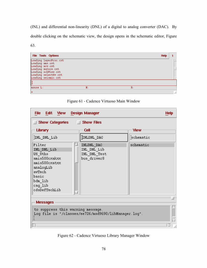
78
(INL) and differential non-linearity (DNL) of a digital to analog converter (DAC). By
double clicking on the schematic view, the design opens in the schematic editor, Figure
63.
Figure 61 - Cadence Virtuoso Main Window
Figure 62 - Cadence Virtuoso Library Manager Window

79
Figure 63 - Cadence Virtuoso Schematic Editor
Again, what is important here is the process, not necessarily the content of the
design. The simulation environment has been saved to two files and they just need to be
retrieved in order to finish setting things up. From the schematic editor view, clicking on
tools and then analog environment will bring up the analog design environment window,
Figure 64. It is from here where the entire simulation environment will be configured.
So far, everything is the exact same no matter if configured to operate on a cluster or not.
Selecting session and then load state brings up a dialog from which a state name
can be restored. Once this has been restored, the analog design environment window
changes to what is shown in Figure 65. Notice the design variables and the outputs have
updated based on the configuration loaded from the state file.

80
Figure 64 - Cadence Virtuoso Analog Design Environment Window
Figure 65 - Cadence Virtuoso Updated Analog Design Environment Window

81
Next, we need to configure the simulation environment. Selecting setup and then
simulator/directory/host from the menu does this. This is the first difference for the
cluster environment. Since all of the settings have previously been configured, the host
mode of distributed can now be selected and will operate properly. By simply changing
the radio button for host mode to distributed from local, as shown in Figure 66, the end
user has done all that is necessary to use the cluster to simulate. Click OK to save the
settings.
Figure 66 - Cadence Virtuoso Simulator/Directory/Host Window
The last thing to set up the simulation is to load the corners file. This is done by
selecting tools and then corners from the analog design environment window. The
analog corners analysis window is now active. Selecting file and then load brings up a
window from which you can browse to select a corners input file. Once selected and
loaded, the corners analysis window should now look like what is show in Figure 67.

82
Figure 67 - Cadence Virtuoso Analog Corners Analysis Window
Cadence uses the term corners to define the individual treatment combinations
that are to be run in a designed experiment. This example is making use of 45 different
treatment combinations or corners. When run on a single workstation with a 2.2GHz 64-
bit X86 processor, it takes about one hour per corner for a total time of just over 45 hours
to produce the graph shown in Figure 68. The simulations are processor bound and don’t
use a significant amount of memory during the simulation process.

83
Figure 68 - Differential Nonlinearity and Integral Nonlinearity of the DAC
Clicking the run button in the analog corners analysis window will bring up one
final dialog window. This is the only other thing that is new to the end user when
running the simulations in a cluster configuration. Figure 69 shows how the analog
distributed processing option window should be configured for SGE. There are plenty of
other options that could be configured for SGE, but for verification, the defaults are fine.
Since all of the simulations in this case are independent of one another, all 45 will be
queued into SGE as soon as they are configured after clicking OK.

84
Figure 69 - Cadence Virtuoso Analog Distributed Processing Window

85
Similar to what was previously shown when looking at the Silvaco Virtual Wafer
Fab simulations, one can run “watch qstat –f” and see the jobs being queued and sent
directly into the nodes for processing. The difference here, again, is that all jobs are
queued and processed immediately. Since the cluster environment that has been installed
has enough processors to handle all 45 simulations simultaneously, the entire simulation
finishes in just over an hour, producing the same graph shown in Figure 68.

86
Chapter 7 Conclusions
This work has demonstrated a method by which a computational cluster can be
built with a focus on the applications used in the microelectronic industry. The
integration of the hardware and software components has led to a system that is easy to
use and easy to maintain.
Installation of a Linux operating system, CentOS, was performed via a method
known as kickstart. Cluster execute nodes were configured to boot from the network and
are able to be installed and added to the working cluster configuration automatically in a
matter of about 20-30 minutes. Storage for the cluster was configured such that backups
of the necessary configuration files for the execution nodes are restored automatically
upon machine reinstall. This produced a framework for system updates to be performed
via reinstalling machines instead of patching. This leads to an environment that is highly
compliant as all machines are sure to have the same configuration since the installations
are scripted.
Software installation procedures for Silvaco Virtual Wafer Fab and Cadence
Virtuoso were documented. Along with those packages, the main distributed resource
manager, Sun Grid Engine, was installed and configured. Each of the software packages
was then configured to work properly within the SGE environment. A network
accessible storage area was provided for SGE that made it easy to configure on all the
execute nodes and provided the best performance and ease-of-configuration trade-off.
Simulations of a typical microelectronic diffusion process were performed under
Silvaco VWF. By simply selecting to use the grid as a network resource instead of a
local one, the end user is able to completely configure the working environment with the

87
changing of one dropdown box. Simulations were automatically queued to the
distributed resource manager, and then SGE took over and scheduled the jobs on the
execute nodes without further user intervention. Results of the diffusion junction depth
were able to be extracted quickly with a few clicks and could be exported to a comma-
separated file for further analysis. Although exact numbers were not calculated, it could
be easily seen that the use of Silvaco VWF under the SGE environment was able to
greatly accelerate the production of results.
Lastly, simulations of a digital to analog converter were performed under Cadence
Virtuoso. The graphs produced under a single workstation simulation run took
approximately 45 hours to produce. To configure the Cadence simulations to run using
the distributed resource manager, a user simply chose to run the simulations distributed
instead of local or remote. Other than that, a user simply had to select to submit the jobs
to the queue when prompted and all was handled automatically. The production of the
final graphs when run on the configured cluster was reduced down to just over an hour.
This resulted in a 98% reduction in the amount of time required to produce the results.

88
Appendix A – Master Node Kickstart File
install cmdline url --url http://mirrors.rit.edu/centos/5/os/x86_64 lang en_US.UTF-8 keyboard us xconfig --defaultdesktop kde network --device eth0 --bootproto dhcp rootpw ChangeMe firewall --enabled --port=22:tcp --trust eth1 authconfig --enablepamaccess --enableshadow --enablemd5 --enableldap --enableldaptls --ldaploadcacert=http://www.ce.rit.edu/files/hermes.pem --ldapserver=hermes.ce.rit.edu --ldapbasedn=dc=vlsi,dc=ce,dc=rit,dc=edu --enablekrb5 --krb5realm=RIT.EDU --krb5kdc=kerberos-1.rit.edu:88,kerberos-2.rit.edu:88 --krb5adminserver= selinux --enforcing timezone --utc America/New_York bootloader --location=mbr reboot clearpart --drives=sda,sdb --all --initlabel part raid.01 --asprimary --size=128 --ondisk=sda part raid.02 --asprimary --size=128 --ondisk=sdb part raid.03 --asprimary --size=2048 --grow --ondisk=sda part raid.04 --asprimary --size=2048 --grow --ondisk=sdb raid /boot --fstype ext3 --level=1 --device=md1 raid.01 raid.02 raid pv.01 --fstype ext3 --level=1 --device=md2 raid.03 raid.04 volgroup vg0 pv.01 logvol swap --fstype swap --name=swap --vgname=vg0 --recommended logvol /usr --fstype ext3 --name=usr --vgname=vg0 --size=8192 logvol /var --fstype ext3 --name=var --vgname=vg0 --size=8192 logvol /tmp --fstype ext3 --name=tmp --vgname=vg0 --size=8192 logvol / --fstype ext3 --name=root --vgname=vg0 --size=1024 --grow %packages @base

89
@base-x @core @editors @graphical-internet @graphics @kde-desktop @printing @sound-and-video @text-internet emacs rdesktop screen iptraf gdb libXp libXmu mesa-libGLU nss_ldap strace gcc-c++ glibc-devel glib2-devel glib kernel-devel freeglut-devel ncurses-devel libusb-devel pkgconfig openmotif elfutils-libelf gnome-vfs2 ncurses compat-db compat-glibc compat-libf2c-34 compat-libstdc++-296 compat-libstdc++-33 cvs subversion vim-X11 libraw1394 tetex-latex pidgin flex bison libtool libXi-devel

90
libXt-devel libXmu-devel xfig gmp tcl tk xorg-x11-server-Xvfb valgrind dhcp tftp-server bind caching-nameserver -nspluginwrapper %post ( chvt 3 set -v . /etc/sysconfig/network hostname ${HOSTNAME} sed -i -e 's|mirrorlist=|#mirrorlist=|' /etc/yum.repos.d/CentOS-Base.repo sed -i -e 's|#baseurl=http://mirror.centos.org|baseurl=http://mirrors.rit.edu|' /etc/yum.repos.d/CentOS-Base.repo yum -y remove yum-updatesd firefox.x86_64 yum -y install yum-cron # ganglia rpm -ivh http://download.fedora.redhat.com/pub/epel/5/x86_64/epel-release-5-3.noarch.rpm sed -i -e 's|mirrorlist=|#mirrorlist=|' /etc/yum.repos.d/epel.repo sed -i -e 's|#baseurl=http://download.fedoraproject.org/pub|baseurl=http://mirrors.rit.edu|' /etc/yum.repos.d/epel.repo cat > /etc/yum.repos.d/epel.repo.patch << "EOF" 8a includepkgs=ganglia* . EOF patch /etc/yum.repos.d/epel.repo /etc/yum.repos.d/epel.repo.patch rm /etc/yum.repos.d/epel.repo.patch yum -y install ganglia-gmetad ganglia-gmond chkconfig gmetad on chkconfig gmond on

91
# Kile, potrace, lyx, x11vnc, and opencv rpm -ivh http://mirrors.rit.edu/dag/redhat/el5/en/x86_64/RPMS.dag/rpmforge-release-0.3.6-1.el5.rf.x86_64.rpm sed -i -e 's|mirrorlist = http|#mirrorlist = http|' /etc/yum.repos.d/rpmforge.repo sed -i -e 's|#baseurl = http://apt.sw.be|baseurl = http://mirrors.rit.edu/dag|' /etc/yum.repos.d/rpmforge.repo echo "includepkgs = kile potrace lyx x11vnc opencv opencv-devel opencv-python" >> /etc/yum.repos.d/rpmforge.repo yum -y install kile potrace lyx x11vnc opencv opencv-devel opencv-python # Adobe Reader and Flash rpm -ivh http://linuxdownload.adobe.com/adobe-release/adobe-release-i386-1.0-1.noarch.rpm # flash-plugin broken in version 10 and 64-bit plugin needs 64-bit browser which gets dumb with nspluginwrapper yum -y install AdobeReader_enu # All to install Java wget -O jre-6u13-linux-i586-rpm.bin http://javadl.sun.com/webapps/download/AutoDL?BundleId=29209 sed -i -e 's|more <<|cat <<|' jre-6u13-linux-i586-rpm.bin chmod 644 /usr/bin/sum echo y | sh ./jre-6u13-linux-i586-rpm.bin chmod 755 /usr/bin/sum ln -svf "$(rpm -ql jre|grep plugin|grep ns7/|grep \\.so$)" /usr/lib/mozilla/plugins/libjavaplugin_oji.so /usr/sbin/alternatives --install /usr/bin/java java $(rpm -ql jre|grep bin/java$) 1 echo 1 | /usr/sbin/alternatives --config java rm -vf jre-6u13-linux-i586* # Done with java install # OpenOffice Install wget --progress=bar:force ftp://ftp.ussg.iu.edu/pub/openoffice/stable/3.0.1/OOo_3.0.1_LinuxIntel_install_en-US.tar.gz tar -xzf OOo_3.0.1_LinuxIntel_install_en-US.tar.gz rpm -Uvhi OO*native*/RPMS/*.rpm rpm -Uvhi OO*native*/RPMS/desktop-integration/*redhat*.rpm rm -vrf OO* # Done with OpenOffice Install yum -y update cat > /etc/yum.repos.d/atrpms.repo << "EOF" [atrpms] name = CentOS $releasever - $basearch - ATrpms

92
baseurl = http://mirrors.rit.edu/atrpms/el$releasever-$basearch/atrpms/stable gpgkey = http://atrpms.net/RPM-GPG-KEY.atrpms gpgcheck = 1 includepkgs = avidemux amrnb libfaac0 libmp3lame0 libsndfile1 libxvidcore4 faad2 jack-audio-connection-kit libfreebob libsamplerate libx264* fftw fftw-devel mplayer aalib liba52_0 libdirect* libdirectfb* libfaad* libfusion* liblirc_client0 liblzo2* libmad0 libxvidcore4 twolame mplayer-fonts svgalib xmms-libs mplayer-skins EOF rpm --import http://atrpms.net/RPM-GPG-KEY.atrpms yum -y install avidemux mplayer mplayer-skins fftw fftw-devel find / -iname '*.rpmnew' | while read i; do mv -vf $i ${i%.rpmnew}; done ln -s /usr/bin/firefox /usr/bin/mozilla /sbin/chkconfig ip6tables off /sbin/chkconfig bluetooth off /sbin/chkconfig avahi-daemon off /sbin/chkconfig hidd off /sbin/chkconfig hplip off /sbin/chkconfig ntpd on /sbin/chkconfig yum-cron on echo "root: [email protected]" >> /etc/aliases echo DISPLAYMANAGER="KDE" >> /etc/sysconfig/desktop sed -i -e 's|usetls="no"|usetls="yes"|' /etc/autofs_ldap_auth.conf sed -i -e 's|tlsrequired="no"|tlsrequired="yes"|' /etc/autofs_ldap_auth.conf sed -i -e 's|umask 002|umask 007|' /etc/bashrc sed -i -e 's|#auth|auth|' /etc/pam.d/su sed -i -e 's|AllowShutdown=All|AllowShutdown=Root|' /usr/share/config/kdm/kdmrc sed -i -e 's|redhat-email|kde-konsole|' /usr/share/config/kickerrc sed -i -e 's|WallpaperMode=Scaled|WallpaperMode=NoWallpaper|' /usr/share/config/kdesktoprc sed -i -e 's|exclude=|exclude=media/nfs_mounted,media/nfs_unmounted,|' /usr/share/config/kdesktoprc echo "schema=Linux.schema" >> /usr/share/config/konsolerc cat >> /usr/share/config/kdeglobals << "EOF" [KDE Resource Restrictions][$i] icon=false

93
wallpaper=false EOF cat > /usr/share/config/kcmdisplayrc << "EOF" [$Version] update_info=kcmdisplayrc.upd:kde3 [DisplayEnergy] displayEnergySaving=true displayPowerOff=30 displayStandby=0 displaySuspend=15 EOF cat > /etc/X11/fs/config.patch << "EOF" 20a /tools/mentor/fonts, . EOF patch /etc/X11/fs/config /etc/X11/fs/config.patch rm /etc/X11/fs/config.patch sed -i -e 's|no-listen = tcp|# no-listen = tcp|' /etc/X11/fs/config cat > /etc/pam.d/system-auth.patch << "EOF" 4a auth optional pam_group.so . EOF patch /etc/pam.d/system-auth /etc/pam.d/system-auth.patch rm /etc/pam.d/system-auth.patch echo "*; *; *; Al0000-2400; lp,uucp" >> /etc/security/group.conf cat > /etc/sysconfig/iptables.patch << "EOF" 18a -I INPUT -m state --state NEW -p tcp --dport ssh -m recent --set -I INPUT -m state --state NEW -p tcp --dport ssh -m recent --update --seconds 300 --hitcount 6 -j DROP . EOF patch /etc/sysconfig/iptables /etc/sysconfig/iptables.patch rm /etc/sysconfig/iptables.patch cat > /etc/sysconfig/iptables.patch << "EOF" 21a -A RH-Firewall-1-INPUT -m state --state NEW -m tcp -p tcp --dport 8649 -j ACCEPT -A RH-Firewall-1-INPUT -m state --state NEW -m udp -p udp --dport 8649 -j ACCEPT

94
-A RH-Firewall-1-INPUT -m state --state NEW -m tcp -p tcp --dport 8652 -j ACCEPT . EOF patch /etc/sysconfig/iptables /etc/sysconfig/iptables.patch rm /etc/sysconfig/iptables.patch echo "ServerName klein.ce.rit.edu" >> /etc/cups/client.conf echo "default pdf" >> /etc/cups/lpoptions mkdir /tools /class /dropbox /shared cat >> /etc/fstab << "EOF" nfs.ce.rit.edu:/export/nfs-tools /tools nfs ro,noatime,rsize=32768,wsize=32768 nfs.ce.rit.edu:/export/nfs-class /class nfs ro,noatime,rsize=32768,wsize=32768 nfs.ce.rit.edu:/export/nfs-dropbox /dropbox nfs rw,noatime,rsize=32768,wsize=32768 nfs.ce.rit.edu:/export/nfs-shared /shared nfs rw,noatime,rsize=32768,wsize=32768 EOF cat > /etc/profile.d/ssh-keygen.sh << "EOF" if [ ! -e $HOME/.ssh/id_rsa.pub ] ; then ssh-keygen -q -t rsa -b 2048 -f $HOME/.ssh/id_rsa -N "" fi if [ ! -e $HOME/.ssh/authorized_keys ] ; then cp $HOME/.ssh/id_rsa.pub $HOME/.ssh/authorized_keys chmod 600 $HOME/.ssh/authorized_keys fi EOF cat > /etc/security/limits.d/90-nproc.conf << "EOF" # Default limit for number of user's processes to prevent # accidental fork bombs. # See rhbz #432903 for reasoning. * soft nproc 1024 EOF cat > /etc/profile.d/tools.sh << "EOF" if ! [ `/usr/bin/id -u` = 0 ] ; then for i in /tools/env.d/*.sh ; do if [ -r "$i" ] ; then . $i fi done unset i fi EOF chmod 755 /etc/profile.d/tools.sh

95
# Setup environment to kickstart machine again # grub> savedefault --default=2 --once ; grub> quit # sed -i -e 's|default=0|default=2|' /boot/grub/grub.conf wget --progress=bar:force -O /boot/initrd-kickstart.img http://mirrors.rit.edu/centos/5/os/x86_64/isolinux/initrd.img wget --progress=bar:force -O /boot/vmlinuz-kickstart http://mirrors.rit.edu/centos/5/os/x86_64/isolinux/vmlinuz cat >> /boot/grub/grub.conf << "EOF" title Kickstart root (hd0,0) kernel /vmlinuz-kickstart ks=nfs:nfs-01:/export/nfs-kickstart/phoenix.cfg ksdevice=eth0 initrd /initrd-kickstart.img EOF # Restore saved data including SSH keys, xorg.conf mkdir /mnt/temp mount nfs-01:/export/nfs-kickstart /mnt/temp -o nolock cp -rv /mnt/temp/${HOSTNAME}/* / umount /mnt/temp rmdir /mnt/temp ) 2>&1 | tee /root/kickstart-post.log chvt 1

96
Appendix B – Compute Node Kickstart File
install cmdline url --url http://mirrors.rit.edu/centos/5/os/x86_64 lang en_US.UTF-8 keyboard us xconfig --defaultdesktop kde network --device eth0 --bootproto dhcp rootpw ChangeMe firewall --disabled authconfig --enablepamaccess --enableshadow --enablemd5 --enableldap --enableldaptls --ldaploadcacert=http://www.ce.rit.edu/files/hermes.pem --ldapserver=hermes.ce.rit.edu --ldapbasedn=dc=vlsi,dc=ce,dc=rit,dc=edu --enablekrb5 --krb5realm=RIT.EDU --krb5kdc=kerberos-1.rit.edu:88,kerberos-2.rit.edu:88 --krb5adminserver= selinux --disabled timezone --utc America/New_York bootloader --location=mbr reboot clearpart --all --initlabel part /boot --fstype ext3 --size=128 part pv.01 --size=0 --grow volgroup vg0 pv.01 logvol swap --fstype swap --name=swap --vgname=vg0 --recommended logvol /usr --fstype ext3 --name=usr --vgname=vg0 --size=8192 logvol /var --fstype ext3 --name=var --vgname=vg0 --size=8192 logvol /tmp --fstype ext3 --name=tmp --vgname=vg0 --size=8192 logvol / --fstype ext3 --name=root --vgname=vg0 --size=8192 logvol /scratch --fstype ext3 --name=scratch --vgname=vg0 --size=1024 --grow %packages @base @base-x @core @editors @graphical-internet @graphics @kde-desktop

97
@printing @sound-and-video @text-internet emacs rdesktop screen iptraf gdb libXp libXmu mesa-libGLU nss_ldap strace gcc-c++ glibc-devel glib2-devel glib kernel-devel freeglut-devel ncurses-devel libusb-devel pkgconfig openmotif elfutils-libelf gnome-vfs2 ncurses compat-db compat-glibc compat-libf2c-34 compat-libstdc++-296 compat-libstdc++-33 cvs subversion vim-X11 libraw1394 tetex-latex pidgin flex bison libtool libXi-devel libXt-devel libXmu-devel xfig gmp tcl tk

98
xorg-x11-server-Xvfb valgrind openmotif22 vnc -nspluginwrapper -krb5-auth-dialog %post ( chvt 3 set -v . /etc/sysconfig/network hostname ${HOSTNAME} sed -i -e 's|mirrorlist=|#mirrorlist=|' /etc/yum.repos.d/CentOS-Base.repo sed -i -e 's|#baseurl=http://mirror.centos.org|baseurl=http://mirrors.rit.edu|' /etc/yum.repos.d/CentOS-Base.repo yum -y remove yum-updatesd yum -y install yum-cron xdg-utils # ganglia and environment-modules rpm -ivh http://mirrors.rit.edu/epel/5/x86_64/epel-release-5-3.noarch.rpm sed -i -e 's|mirrorlist=|#mirrorlist=|' /etc/yum.repos.d/epel.repo sed -i -e 's|#baseurl=http://download.fedoraproject.org/pub|baseurl=http://mirrors.rit.edu|' /etc/yum.repos.d/epel.repo cat > /etc/yum.repos.d/epel.repo.patch << "EOF" 8a includepkgs=ganglia* environment-modules . EOF patch /etc/yum.repos.d/epel.repo /etc/yum.repos.d/epel.repo.patch rm /etc/yum.repos.d/epel.repo.patch yum -y install ganglia-gmond environment-modules chkconfig gmond on # Kile, potrace, lyx, x11vnc, and opencv rpm -ivh http://mirrors.rit.edu/dag/redhat/el5/en/x86_64/RPMS.dag/rpmforge-release-0.3.6-1.el5.rf.x86_64.rpm sed -i -e 's|mirrorlist = http|#mirrorlist = http|' /etc/yum.repos.d/rpmforge.repo sed -i -e 's|#baseurl = http://apt.sw.be|baseurl = http://mirrors.rit.edu/dag|' /etc/yum.repos.d/rpmforge.repo

99
echo "includepkgs = kile potrace lyx x11vnc opencv opencv-devel opencv-python djvulibre" >> /etc/yum.repos.d/rpmforge.repo yum -y install kile potrace lyx x11vnc opencv opencv-devel opencv-python djvulibre # Adobe Reader rpm -ivh http://linuxdownload.adobe.com/adobe-release/adobe-release-i386-1.0-1.noarch.rpm yum -y install AdobeReader_enu # All to install Java wget -O jre-6u15-linux-x64-rpm.bin http://javadl.sun.com/webapps/download/AutoDL?BundleId=33226 sed -i -e 's|more <<|cat <<|' jre-6u15-linux-x64-rpm.bin chmod 644 /usr/bin/sum echo y | sh ./jre-6u15-linux-x64-rpm.bin chmod 755 /usr/bin/sum ln -svf /usr/java/default/lib/amd64/libnpjp2.so /usr/lib64/mozilla/plugins/libnpjp2.so /usr/sbin/alternatives --install /usr/bin/java java $(rpm -ql jre|grep bin/java$) 1 echo 1 | /usr/sbin/alternatives --config java rm -vf jre-6u15-linux-* # Done with java install # OpenOffice Install wget --progress=bar:force ftp://ftp.ussg.iu.edu/pub/openoffice/stable/3.1.0/OOo_3.1.0_LinuxX86-64_install_en-US.tar.gz tar -xzf OOo_3.1.0_LinuxX86-64_install_en-US.tar.gz rpm -Uvhi OO*native*/RPMS/*.rpm rpm -Uvhi OO*native*/RPMS/desktop-integration/*redhat*.rpm rm -vrf OO* # Done with OpenOffice Install yum -y update cat > /etc/yum.repos.d/atrpms.repo << "EOF" [atrpms] name = CentOS $releasever - $basearch - ATrpms baseurl = http://mirrors.rit.edu/atrpms/el$releasever-$basearch/atrpms/stable gpgkey = http://atrpms.net/RPM-GPG-KEY.atrpms gpgcheck = 1 includepkgs = avidemux amrnb libfaac0 libmp3lame0 libsndfile1 libxvidcore4 faad2 jack-audio-connection-kit libfreebob libsamplerate libx264* fftw fftw-devel mplayer aalib liba52_0 libdirect* libdirectfb* libfaad* libfusion* liblirc_client0 liblzo2* libmad0 libxvidcore4 twolame mplayer-fonts svgalib xmms-libs mplayer-skins

100
EOF rpm --import http://atrpms.net/RPM-GPG-KEY.atrpms yum -y install avidemux mplayer mplayer-skins fftw fftw-devel find / -iname '*.rpmnew' | while read i; do mv -vf $i ${i%.rpmnew}; done ln -s /usr/bin/firefox /usr/bin/mozilla /sbin/chkconfig ip6tables off /sbin/chkconfig bluetooth off /sbin/chkconfig avahi-daemon off /sbin/chkconfig hidd off /sbin/chkconfig hplip off /sbin/chkconfig ntpd on /sbin/chkconfig yum-cron on echo "root: [email protected]" >> /etc/aliases echo DISPLAYMANAGER="KDE" >> /etc/sysconfig/desktop sed -i -e 's|usetls="no"|usetls="yes"|' /etc/autofs_ldap_auth.conf sed -i -e 's|tlsrequired="no"|tlsrequired="yes"|' /etc/autofs_ldap_auth.conf sed -i -e 's|umask 002|umask 007|' /etc/bashrc sed -i -e 's|#auth|auth|' /etc/pam.d/su sed -i -e 's|AllowShutdown=All|AllowShutdown=Root|' /usr/share/config/kdm/kdmrc sed -i -e 's|redhat-email|kde-konsole|' /usr/share/config/kickerrc sed -i -e 's|WallpaperMode=Scaled|WallpaperMode=NoWallpaper|' /usr/share/config/kdesktoprc sed -i -e 's|exclude=|exclude=media/nfs_mounted,media/nfs_unmounted,|' /usr/share/config/kdesktoprc echo "schema=Linux.schema" >> /usr/share/config/konsolerc cat >> /usr/share/config/kdeglobals << "EOF" [KDE Resource Restrictions][$i] icon=false wallpaper=false EOF cat > /usr/share/config/kcmdisplayrc << "EOF" [$Version] update_info=kcmdisplayrc.upd:kde3 [DisplayEnergy] displayEnergySaving=true displayPowerOff=30 displayStandby=0

101
displaySuspend=15 EOF chmod +s /sbin/mount.cifs chmod +s /sbin/umount.cifs cat > /etc/X11/fs/config.patch << "EOF" 20a /tools/mentor/fonts, . EOF patch /etc/X11/fs/config /etc/X11/fs/config.patch rm /etc/X11/fs/config.patch sed -i -e 's|no-listen = tcp|# no-listen = tcp|' /etc/X11/fs/config cat > /etc/pam.d/system-auth.patch << "EOF" 4a auth optional pam_group.so . EOF patch /etc/pam.d/system-auth /etc/pam.d/system-auth.patch rm /etc/pam.d/system-auth.patch echo "*; *; *; Al0000-2400; lp,uucp" >> /etc/security/group.conf echo "#-:ALL EXCEPT root vip:ALL" >> /etc/security/access.conf echo "ServerName klein.ce.rit.edu" >> /etc/cups/client.conf echo "default pdf" >> /etc/cups/lpoptions mkdir /tools /class /dropbox /shared cat >> /etc/fstab << "EOF" nfs-01.local:/export/nfs-tools /tools nfs ro,noatime,rsize=32768,wsize=32768 nfs-01.local:/export/nfs-class /class nfs ro,noatime,rsize=32768,wsize=32768 nfs-01.local:/export/nfs-dropbox /dropbox nfs rw,noatime,rsize=32768,wsize=32768 nfs-01.local:/export/nfs-shared /shared nfs rw,noatime,rsize=32768,wsize=32768 EOF cat > /etc/profile.d/ssh-keygen.sh << "EOF" if [ ! -e $HOME/.ssh/id_rsa.pub ] ; then ssh-keygen -q -t rsa -b 2048 -f $HOME/.ssh/id_rsa -N "" fi if [ ! -e $HOME/.ssh/authorized_keys ] ; then cp $HOME/.ssh/id_rsa.pub $HOME/.ssh/authorized_keys chmod 600 $HOME/.ssh/authorized_keys fi EOF

102
sed -i -e 's|#Banner /some/path|Banner /etc/ssh/banner|' /etc/ssh/sshd_config cat > /etc/ssh/banner << "EOF" ******************************************************************** Authorized Users only. Please use your RIT account to log in. ******************************************************************** EOF cat > /etc/security/limits.d/90-nproc.conf << "EOF" # Default limit for number of user's processes to prevent # accidental fork bombs. # See rhbz #432903 for reasoning. * soft nproc 1024 EOF # Configure system to use environment-modules # ln -sf /tools/Modules/init/bash /etc/profile.d/modules.sh # ln -sf /tools/Modules/init/csh /etc/profile.d/modules.csh # cat > /etc/profile.d/tools.sh << "EOF" if ! [ `/usr/bin/id -u` = 0 ] ; then for i in /tools/env.d/*.sh ; do if [ -r "$i" ] ; then . $i fi done unset i fi EOF chmod 755 /etc/profile.d/tools.sh # Setup environment to kickstart machine again # grub> savedefault --default=2 --once ; grub> quit # sed -i -e 's|default=0|default=2|' /boot/grub/grub.conf wget --progress=bar:force -O /boot/initrd-kickstart.img http://mirrors.rit.edu/centos/5/os/x86_64/isolinux/initrd.img wget --progress=bar:force -O /boot/vmlinuz-kickstart http://mirrors.rit.edu/centos/5/os/x86_64/isolinux/vmlinuz cat >> /boot/grub/grub.conf << "EOF" title Kickstart root (hd0,0) kernel /vmlinuz-kickstart ks=nfs:nfs-01.local:/export/nfs-kickstart/node.cfg ksdevice=eth0 initrd /initrd-kickstart.img EOF

103
# Install SGE mkdir /home/sge mount nfs-01.local:/export/nfs-home/sge /home/sge -o nolock source /home/sge/6.2u3/default/common/settings.sh cd $SGE_ROOT ./install_execd -noremote -auto util/install_modules/sge_configuration.conf ln -sf /home/sge/6.2u3/default/common/settings.sh /etc/profile.d/sge.sh ln -sf /home/sge/6.2u3/default/common/settings.csh /etc/profile.d/sge.csh cd / umount /home/sge rmdir /home/sge # Restore saved data including SSH keys mkdir /mnt/temp mount nfs-01.local:/export/nfs-kickstart /mnt/temp -o nolock cp -rv /mnt/temp/${HOSTNAME}/* / umount /mnt/temp rmdir /mnt/temp chmod 1777 /scratch ntpdate -s ntp.rit.edu ) 2>&1 | tee /root/kickstart-post.log chvt 1

104
Appendix C – Sun Grid Engine Configuration File
#------------------------------------------------- # SGE configuration file #------------------------------------------------- # Use always fully qualified pathnames, please # SGE_ROOT Path, this is basic information #(mandatory for qmaster and execd installation) SGE_ROOT="/home/sge/6.2u3" # SGE_QMASTER_PORT is used by qmaster for communication # Please enter the port in this way: 1300 # Please do not this: 1300/tcp #(mandatory for qmaster installation) SGE_QMASTER_PORT="6444" # SGE_EXECD_PORT is used by execd for communication # Please enter the port in this way: 1300 # Please do not this: 1300/tcp #(mandatory for qmaster installation) SGE_EXECD_PORT="6445" # CELL_NAME, will be a dir in SGE_ROOT, contains the common dir # Please enter only the name of the cell. No path, please #(mandatory for qmaster and execd installation) CELL_NAME="default" # ADMIN_USER, if you want to use a different admin user than the owner, # of SGE_ROOT, you have to enter the user name, here # Leaving this blank, the owner of the SGE_ROOT dir will be used as admin user ADMIN_USER="" # The dir, where qmaster spools this parts, which are not spooled by DB #(mandatory for qmaster installation) QMASTER_SPOOL_DIR="/home/sge/default/spool/qmaster" # The dir, where the execd spools (active jobs) # This entry is needed, even if your are going to use # berkeley db spooling. Only cluster configuration and jobs will

105
# be spooled in the database. The execution daemon still needs a spool # directory #(mandatory for qmaster installation) EXECD_SPOOL_DIR="/home/sge/default/spool" # For monitoring and accounting of jobs, every job will get # unique GID. So you have to enter a free GID Range, which # is assigned to each job running on a machine. # If you want to run 100 Jobs at the same time on one host you # have to enter a GID-Range like that: 16000-16100 #(mandatory for qmaster installation) GID_RANGE="200000-200100" # If SGE is compiled with -spool-dynamic, you have to enter here, which # spooling method should be used. (classic or berkeleydb) #(mandatory for qmaster installation) SPOOLING_METHOD="classic" # Name of the Server, where the Spooling DB is running on # if spooling methode is berkeleydb, it must be "none", when # using no spooling server and it must containe the servername # if a server should be used. In case of "classic" spooling, # can be left out DB_SPOOLING_SERVER="none" # The dir, where the DB spools # If berkeley db spooling is used, it must contain the path to # the spooling db. Please enter the full path. (eg. /tmp/data/spooldb) # Remember, this directory must be local on the qmaster host or on the # Berkeley DB Server host. No NFS mount, please DB_SPOOLING_DIR="/home/sge/default/spooldb" # A List of Host which should become admin hosts # If you do not enter any host here, you have to add all of your hosts # by hand, after the installation. The autoinstallation works without # any entry

106
ADMIN_HOST_LIST="" # A List of Host which should become submit hosts # If you do not enter any host here, you have to add all of your hosts # by hand, after the installation. The autoinstallation works without # any entry SUBMIT_HOST_LIST="" # A List of Host which should become exec hosts # If you do not enter any host here, you have to add all of your hosts # by hand, after the installation. The autoinstallation works without # any entry # (mandatory for execution host installation) EXEC_HOST_LIST="`hostname`" # The dir, where the execd spools (local configuration) # If you want configure your execution daemons to spool in # a local directory, you have to enter this directory here. # If you do not want to configure a local execution host spool directory # please leave this empty EXECD_SPOOL_DIR_LOCAL="/home/sge/default/spool" # If true, the domainnames will be ignored, during the hostname resolving # if false, the fully qualified domain name will be used for name resolving HOSTNAME_RESOLVING="true" # Shell, which should be used for remote installation (rsh/ssh) # This is only supported, if your hosts and rshd/sshd is configured, # not to ask for a password, or promting any message. SHELL_NAME="ssh" # Enter your default domain, if you are using /etc/hosts or NIS configuration DEFAULT_DOMAIN="none" # If a job stops, fails, finish, you can send a mail to this adress ADMIN_MAIL="none"

107
# If true, the rc scripts (sgemaster, sgeexecd, sgebdb) will be added, # to start automatically during boottime ADD_TO_RC="true" #If this is "true" the file permissions of executables will be set to 755 #and of ordenary file to 644. SET_FILE_PERMS="true" # This option is not implemented, yet. # When a exechost should be uninstalled, the running jobs will be rescheduled RESCHEDULE_JOBS="wait" # Enter a one of the three distributed scheduler tuning configuration sets # (1=normal, 2=high, 3=max) SCHEDD_CONF="1" # The name of the shadow host. This host must have read/write permission # to the qmaster spool directory # If you want to setup a shadow host, you must enter the servername # (mandatory for shadowhost installation) SHADOW_HOST="" # Remove this execution hosts in automatic mode # (mandatory for unistallation of execution hosts) EXEC_HOST_LIST_RM="" # This option is used for startup script removing. # If true, all rc startup scripts will be removed during # automatic deinstallation. If false, the scripts won't # be touched. # (mandatory for unistallation of execution/qmaster hosts) REMOVE_RC="true" # This is a Windows specific part of the auto isntallation template # If you going to install windows executions hosts, you have to enable the # windows support. To do this, please set the WINDOWS_SUPPORT variable # to "true". ("false" is disabled)

108
# (mandatory for qmaster installation, by default WINDOWS_SUPPORT is # disabled) WINDOWS_SUPPORT="false" # Enabling the WINDOWS_SUPPORT, recommends the following parameter. # The WIN_ADMIN_NAME will be added to the list of SGE managers. # Without adding the WIN_ADMIN_NAME the execution host installation # won't install correctly. # WIN_ADMIN_NAME is set to "Administrator" which is default on most # Windows systems. In some cases the WIN_ADMIN_NAME can be prefixed with # the windows domain name (eg. DOMAIN+Administrator) # (mandatory for qmaster installation) WIN_ADMIN_NAME="Administrator"

109
Bibliography
1 Phillip Allen, “The Practice of Analog IC Design,” IEEE Santa Clara Valley
Solid-State Circuits Chapter, May 13, 2004
2 Brian Bailey, Grant Martin and Andrew Piziali, “ESL Design and Verification:
A Prescription for Electronic System Level Methodology,” 2007, Morgan
Kaufmann/Elsevier
3 Lavagno, Martin, and Scheffer, “Electronic Design Automation For Integrated
Circuits Handbook,” 2006, CRC Taylor & Francis
4 Information Technology Association of America, “Information Technology
Definitions,” 2008,
http://www.itaa.org/es/docs/Information%20Technology%20Definitions.pdf
5 Intel Corporation, “Intel Microprocessor Quick Reference Guide,” 2009,
http://www.intel.com/pressroom/kits/quickrefyr.htm
6 C. Schluting, “Unix or Windows, Operating System Selection Factors,” 2005,
http://www.serverwatch.com/tutorials/article.php/3559086/
7 Silvaco Data Systems INC, “Silvaco – Platform Support,” 2009,
http://www.silvaco.com/support/platforms.html
8 Computer Service Technology INC, “Memory Trends 2008,” 2008,
http://www.simmtester.com/PAGE/news/showpubnews.asp?num=158
9 Sun Microsystems, INC, “SunSoft introduces first shrink-wrapped distributed
computing solution: Solaris,” 1991,
http://www.sun.com/aboutsun/media/presskits/25years/pr.html#solaris

110
10 Free Software Foundation, INC, “GNU General Public License,” 1991,
http://www.gnu.org/licenses/gpl-2.0.txt
11 The CentOS Project, “CentOS Homepage,” 2009, http://www.centos.org/
12 Sapiro, S. and Smith, R. J. “Handbook of Design Automation,” 1986, Prentice-
Hall, Inc.
13 Red Hat, INC, “Red Hat Enterprise Linux 5 Installation Guide,” 2009,
http://www.redhat.com/docs/en-
US/Red_Hat_Enterprise_Linux/5/pdf/Installation_Guide.pdf
14 Rocks Core Development, “Rocks Clusters: About,” 2009,
http://www.rocksclusters.org/wordpress/?page_id=57
15 Sun Microsystems, INC, “Sun Grid Engine 6.2u3,” 2009,
http://wikis.sun.com/display/gridengine62u3/
16 Sun Microsystems, INC, “Using ssh with qrsh and qlogin,” 2009,
http://gridengine.sunsource.net/howto/qrsh_qlogin_ssh.html
17 Silvaco Data Systems, INC, “Standard Floating License Manager: Installation
and User’s Guide,” April 17, 2006,
https://dynamic.silvaco.com/dynamicweb/smcen/downloadFiles/installationManuals/sflm
7_install_users.pdf
18 Sun Microsystems, INC, “How the System Operates,” 2009,
http://wikis.sun.com/display/gridengine62u3/How+the+System+Operates
19 Silvaco Data Systems, INC, “VWF User’s Manual,” April 1, 2009,
vwf_users1.pdf

111
20 Cadence Design Systems, INC, “Cadence Design Framework II Configuration
Guide,” Version 5.0, March 2007, dfIIconfig.pdf