DESIGN AND IMPLEMENTATION OF A …sirius.cs.put.poznan.pl/...DiagnosisToolUsingBayesianNetworks.pdffor a specialised diagnosis service arose which would give the management system

Poznan University of Technology

Faculty of Computing Science

Institute of Computing Science

Master’s thesis

DESIGN AND IMPLEMENTATION OF A COMPUTER SYSTEMSDIAGNOSIS TOOL USING BAYESIAN NETWORKS

Bartosz Kosarzycki

Supervisor

Michał Sajkowski, Ph. D.

Poznan 2011

Replace this page with Master’s thesis summary card;

The original version goes to PUT archives, other copies receive b&w copy of the card.

Contents

1 Introduction 71.1 Motivation . . . . . . . . . . . . . . . . . . . . . . . . . . . . . . . . . . . . . . 7

1.2 Introduction to Bayesian networks . . . . . . . . . . . . . . . . . . . . . . . . . 8

1.3 The purpose and scope of work . . . . . . . . . . . . . . . . . . . . . . . . . . . 8

1.4 Contents of this thesis . . . . . . . . . . . . . . . . . . . . . . . . . . . . . . . 9

2 Theoretical background 112.1 Basic concepts and formulas . . . . . . . . . . . . . . . . . . . . . . . . . . . . 11

2.1.1 Conditional probabilities . . . . . . . . . . . . . . . . . . . . . . . . . . 11

Joint probability distribution . . . . . . . . . . . . . . . . . . . . . . . . 11

Marginal probability . . . . . . . . . . . . . . . . . . . . . . . . . . . . 12

Conditional probability: . . . . . . . . . . . . . . . . . . . . . . . . . . 12

2.1.2 Sum rule, product rule . . . . . . . . . . . . . . . . . . . . . . . . . . . 12

Sum rule . . . . . . . . . . . . . . . . . . . . . . . . . . . . . . . . . . 12

Product rule . . . . . . . . . . . . . . . . . . . . . . . . . . . . . . . . . 12

2.1.3 Bayes’ theorem . . . . . . . . . . . . . . . . . . . . . . . . . . . . . . . 13

2.2 Bayesian networks . . . . . . . . . . . . . . . . . . . . . . . . . . . . . . . . . 13

2.3 Types of reasoning in Bayesian networks . . . . . . . . . . . . . . . . . . . . . . 13

2.4 Causal and evidential reasoning . . . . . . . . . . . . . . . . . . . . . . . . . . 14

2.4.1 Definitions . . . . . . . . . . . . . . . . . . . . . . . . . . . . . . . . . 14

2.4.2 Causality in Bayesian networks . . . . . . . . . . . . . . . . . . . . . . 14

2.5 Basic assumptions in Bayesian networks . . . . . . . . . . . . . . . . . . . . . . 15

2.5.1 Independence of variables based on graph structure . . . . . . . . . . . . 15

Independence example . . . . . . . . . . . . . . . . . . . . . . . . . . . 15

2.5.2 Probability P(X) of a given node . . . . . . . . . . . . . . . . . . . . . . 15

Example . . . . . . . . . . . . . . . . . . . . . . . . . . . . . . . . . . 16

2.5.3 Other properties of Bayesian networks . . . . . . . . . . . . . . . . . . . 16

Joint probability of events . . . . . . . . . . . . . . . . . . . . . . . . . 16

Joint probability of selected events . . . . . . . . . . . . . . . . . . . . . 16

Other examples . . . . . . . . . . . . . . . . . . . . . . . . . . . . . . . 17

2.5.4 Empirical priors in Bayesian networks . . . . . . . . . . . . . . . . . . . 17

2.6 D-separation . . . . . . . . . . . . . . . . . . . . . . . . . . . . . . . . . . . . . 18

2.6.1 D-separation rules . . . . . . . . . . . . . . . . . . . . . . . . . . . . . 18

D-separation example . . . . . . . . . . . . . . . . . . . . . . . . . . . 18

3

Contents

2.7 Bayesian inference . . . . . . . . . . . . . . . . . . . . . . . . . . . . . . . . . 19

2.7.1 Inference algorithms . . . . . . . . . . . . . . . . . . . . . . . . . . . . 19

2.7.2 Bayesian inference example . . . . . . . . . . . . . . . . . . . . . . . . 20

Example network with node probabilities and CPTs . . . . . . . . . . . . 20

Reasoning . . . . . . . . . . . . . . . . . . . . . . . . . . . . . . . . . . 21

Computations . . . . . . . . . . . . . . . . . . . . . . . . . . . . . . . 22

2.8 Conditional probability table . . . . . . . . . . . . . . . . . . . . . . . . . . . . 25

2.9 Markov chains . . . . . . . . . . . . . . . . . . . . . . . . . . . . . . . . . . . . 26

2.9.1 Formal definition . . . . . . . . . . . . . . . . . . . . . . . . . . . . . . 26

Markov chain transition probability table . . . . . . . . . . . . . . . . . 26

Markov chain directed graph . . . . . . . . . . . . . . . . . . . . . . . . 27

Periodicity, Recurrence, Ergodicity . . . . . . . . . . . . . . . . . . . . 27

2.9.2 Stationary Markov chains (Time-homogeneous Markov chains) . . . . . 28

2.10 GIBBS sampling . . . . . . . . . . . . . . . . . . . . . . . . . . . . . . . . . . 28

2.10.1 From sequence of samples to joint distribution . . . . . . . . . . . . . . 29

2.10.2 Sampling algorithm operation . . . . . . . . . . . . . . . . . . . . . . . 29

3 Bayesian diagnostic tool 313.1 System architecture . . . . . . . . . . . . . . . . . . . . . . . . . . . . . . . . . 32

3.1.1 System components . . . . . . . . . . . . . . . . . . . . . . . . . . . . 32

3.1.2 Service specification . . . . . . . . . . . . . . . . . . . . . . . . . . . . 32

3.1.3 REST methods . . . . . . . . . . . . . . . . . . . . . . . . . . . . . . . 33

3.1.4 SOAP methods . . . . . . . . . . . . . . . . . . . . . . . . . . . . . . . 34

3.1.5 Policy access XMLs . . . . . . . . . . . . . . . . . . . . . . . . . . . . 34

Clientaccesspolicy.xml . . . . . . . . . . . . . . . . . . . . . . . . . . . 34

Crossdomain.xml . . . . . . . . . . . . . . . . . . . . . . . . . . . . . . 35

3.1.6 Using REST and SOAP for inference in Bayes Server . . . . . . . . . . 35

3.2 Algorithms used . . . . . . . . . . . . . . . . . . . . . . . . . . . . . . . . . . . 36

3.2.1 Bayesian inference algorithm . . . . . . . . . . . . . . . . . . . . . . . 36

3.2.2 Sampling algorithm . . . . . . . . . . . . . . . . . . . . . . . . . . . . . 37

3.2.3 Best VOI test selection algorithms . . . . . . . . . . . . . . . . . . . . . 38

Description of algorithms . . . . . . . . . . . . . . . . . . . . . . . . . 39

Exhaustive Search (ES) algorithm . . . . . . . . . . . . . . . . . . . . . 40

3.3 Communication languages . . . . . . . . . . . . . . . . . . . . . . . . . . . . . 42

3.3.1 Graph list - communication XML . . . . . . . . . . . . . . . . . . . . . 42

3.3.2 Graph - communication XML . . . . . . . . . . . . . . . . . . . . . . . 42

Conditional probability tables in Graph XML . . . . . . . . . . . . . . . 43

Graph example XML . . . . . . . . . . . . . . . . . . . . . . . . . . . . 44

3.3.3 Fault ranking - communication XML . . . . . . . . . . . . . . . . . . . 45

3.3.4 Best VOI test ranking - communication XML . . . . . . . . . . . . . . . 46

3.3.5 Operation status - communication XML . . . . . . . . . . . . . . . . . . 46

3.3.6 BIF format version 0.3 . . . . . . . . . . . . . . . . . . . . . . . . . . . 47

BIF conditional probability tables . . . . . . . . . . . . . . . . . . . . . 47

4

BIF example . . . . . . . . . . . . . . . . . . . . . . . . . . . . . . . . 47

BIF import . . . . . . . . . . . . . . . . . . . . . . . . . . . . . . . . . 48

3.4 Bayesian networks and CPTs graphical representation . . . . . . . . . . . . . . 50

3.5 Technologies used . . . . . . . . . . . . . . . . . . . . . . . . . . . . . . . . . . 52

3.5.1 Bayes server technologies . . . . . . . . . . . . . . . . . . . . . . . . . 53

SMILE library . . . . . . . . . . . . . . . . . . . . . . . . . . . . . . . 53

3.5.2 Bayes client technologies . . . . . . . . . . . . . . . . . . . . . . . . . . 57

3.6 Bayes Server and Client manual . . . . . . . . . . . . . . . . . . . . . . . . . . 58

3.6.1 Basic functionality . . . . . . . . . . . . . . . . . . . . . . . . . . . . . 58

3.6.2 Manual . . . . . . . . . . . . . . . . . . . . . . . . . . . . . . . . . . . 58

3.6.3 Bayes Client user interface . . . . . . . . . . . . . . . . . . . . . . . . . 59

3.6.4 Bayes Server user interface . . . . . . . . . . . . . . . . . . . . . . . . . 60

3.6.5 VOI tests and MPF ranking . . . . . . . . . . . . . . . . . . . . . . . . 60

3.6.6 Multiple users . . . . . . . . . . . . . . . . . . . . . . . . . . . . . . . 61

3.6.7 Console log . . . . . . . . . . . . . . . . . . . . . . . . . . . . . . . . . 61

Sample console log: . . . . . . . . . . . . . . . . . . . . . . . . . . . . 62

Sample inference using Bayes Client . . . . . . . . . . . . . . . . . . . 62

3.7 Implementation final remarks . . . . . . . . . . . . . . . . . . . . . . . . . . . . 63

3.8 Acknowledgments . . . . . . . . . . . . . . . . . . . . . . . . . . . . . . . . . 64

3.9 C# code of the algorithms used . . . . . . . . . . . . . . . . . . . . . . . . . . . 64

3.9.1 Bayes server . . . . . . . . . . . . . . . . . . . . . . . . . . . . . . . . 64

3.9.2 Bayes client . . . . . . . . . . . . . . . . . . . . . . . . . . . . . . . . . 64

4 Conclusions 67

Appendix:Abbreviations 69

Bibliography 71

5

Chapter 1

Introduction

Diagnostic systems are becoming more popular and accurate. They help physicians as well as sci-

entists perform differential diagnosis. The crucial part of every diagnostic system is its reasoning

engine which relies on data. The input information comes from statistical data as well documented

studies. Executed tests’ reliability is critical in medicine as well as in computer science. There

are no certain tests, however. To minimize false-positive impact of executed tests one can do them

twice before supplying information to the diagnostic system. One of the possible implementa-

tions of reasoning engines are Bayesian networks. In this type of reasoning the information one

supplies on the executed tests is final. The standard definition of BNs includes only two possible

outcomes: positive and negative.

The following section describes Bayesian networks properties and impact. Reasoning example

is given in chapter containing theoretical background.

1.1 Motivation

SOA architecture, among many other virtues, encourages functional software division into ser-

vices. This enables business oriented partitioning, service cloning and on-the-fly service attach.

While the system grows, however, it becomes more and more sophisticated. Software bugs might

result in the failure of entire components. Fortunately, the vast connection net between services in

a distributed processing system can be easily converted into a directed graph.

An example of such a system is the M3 project (Metrics, Monitoring, Management) from

IT-SOA. It is a set of modules for monitoring and management of SOA systems. Its main as-

sumption is to keep the most up to date knowledge of the managed resources (components) and

dependencies between them [1]. Thus the system provides the exact information on which system

services have crashed. Going a step further one would want to know the root causes of failure, not

only its symptoms. Bayesian networks are a perfect solution for this task. This is where a need

for a specialised diagnosis service arose which would give the management system the ability to

predict failure causes with appropriate probabilities.

The Bayesian Tool (BT) is intended to aid automated software and hardware diagnosis in-

side the M3 framework [1]. File in a specific format should be sufficient to aid the diagnosis of

a single hardware/software configuration. Many clients should be able to connect to the service

via SOAP and REST simultaneously. A graphical client for this purpose using SOAP protocol

7

Introduction

will be shipped with the BT software. The Bayesian server should provide extensive logging and

algorithm selection.

1.2 Introduction to Bayesian networks

Bayesian network (BN) is one of the graph representations for modeling uncertainty. A Bayesian

Network can depict a relationship between a disease and its symptoms, machine failure and its root

causes or predict the most probable output passed through a noisy channel. In other words BNs

are a structured, compact directed acyclic graphs (DAGs) which illustrate a problem that is too

large or complex to be represented with tables or equations. Guaranteed consistency is Bayesian

Networks’ main strength among many other virtues such as the existence of efficient algorithms

for computing probabilities without the need to compute the underlying probability distributions

that would be computationally exacting. BNs are a ubiquitous tool for modeling and a framework

for probabilistic calculations.

Bayesian network can be described by:

• a directed acyclic graph which is the structure of BN that enables one to reflect dependencies

between components of the system in question

• conditional probability table (CPT) for each node with a positive input degree. CPTs de-

scribe the relation between a given node and its parents

Thanks to their simple interpretation, consistence and compact way of presenting probabilistic

relations, Bayesian networks became a practical framework for commonsense reasoning under

uncertainty and receive considerable attention in the fields of computer science, cognitive science,

statistics and philosophy [2].

Bayesian Networks have many applications, apart from the ones mentioned above. These

include the usage in computational biology, bio-informatics, medical diagnosis, document classi-

fication, image processing, image restoration and decision support systems.

One cannot ignore the immense importance of BNs in today’s world filled with data and lack-

ing appropriate tools as well as processing power.

1.3 The purpose and scope of work

Author of this work chose Bayesian networks as his Master’s thesis subject mainly because it was

strongly connected with his speciality - the Intelligent Decision Support. The important factor

was also the growing popularity and ease of use of Bayesian networks in drawing accurate and

complicated conclusions. The Bayesian tool project was done as a continuation of an earlier work

in IT-SOA grant [3].

The purpose of work is to design and implement a computer systems diagnosis tool that pro-

vides a mechanism capable of stating the root cause of failure based on several observations. The

symptoms might originate from sensors but the input mechanism is always a file in a text format.

8

1.4. Contents of this thesis

The tool should enable the definition of relation between system components and sensors

in a unique format (relation between parts that can be broken and tests that could be performed

in order to identify the failure, along with appropriate conditional probability tables).

The implemented software should be able to build a Bayesian network given a file in unique

format. Furthermore it should enable inference and visualisation of current network’s state through

a unified interface (API) as well as have a modular design and be compliant with SOA architecture.

1.4 Contents of this thesis

Master’s thesis structure is as follows. In chapter 2 theoretical background is presented. One

learns basic conditional probability notions in this part. This is followed by Bayes’ theorem and

the definition of d-separation test. Next, the Bayesian inference is explained.

Chapter 3.1 describes the system’s architecture, especially the REST and SOAP methods.

Bayes server operation description can be found in chapter 3.2 which includes the use of simple

inference algorithm as well as the use of sampling algorithms.

Chapter 3.3 describes the communication language that is used by REST and SOAP. BIF for-

mat is described in this chapter as well.

Bayesian network and CPTs graphical representation is described in chapter 3.4.

Chapter 3.5 describes the technologies used in the implementation of Bayesian tool.

Chapter 3.6 is a classic manual for Bayes server and Bayes client.

Conclusions, information on C# code and Abbreviations that were used throughout this paper

are described in chapters 4, 3.9 and 4 respectively.

9

Chapter 2

Theoretical background

This section presents concepts connected with probability that are essential for understanding the

basis of Bayesian tool internals. In the first part few basic definitions, laws and rules are described.

Section 2.3 deals with types of reasoning and section 2.4 with causality in Bayesian networks.

Computations of the probability of exemplary events are shown in section 2.5. Section 2.7.2

is intended to explain how Bayesian networks work and provide an easy tutorial on reasoning.

2.1 Basic concepts and formulas

Formulas and notions presented in this section are needed to fully understand Bayesian networks

operation. Some prior knowledge on probability is assumed. Especially the concepts of: random

variable, probability distribution, discrete sample space and set theory should be familiar to the

reader. Refer to book [4] for further explanation.

2.1.1 Conditional probabilities

The probability P(X) denotes the likelihood of a certain event while P(X|Y) refers to the probabil-

ity of event X, given the occurrence of some other event Y. Consequently event X is conditional

upon event Y. In a probabilistic situation the unconditioned probability P(X) has to be reduced to

the outcomes where Y has a certain value (in this case is true) in order to create P(X|Y). Condi-

tional probabilities are thoroughly described in book [5].

Joint probability distribution

The joint probability distribution is a multivariate distribution of random variables defined on the

same probability space. The cumulative distribution for joint probability of two random variables

is defined as: F(x,y) = P(X < x, Y < y). In computer science one deals mostly with discrete

variables. Simplifying, the probability of two events occurring at the same time (X = x, Y = y) or

in other words the probability of two components being in certain states (x, y) will be: P(X,Y),also depicted as P(X ∩Y ).

11


Marginal probability

Given the joint probabilities of X and Y the marginal probability can be computed by summing

joint probabilities over X or Y. For discrete random variables, the marginal function can be writ-

ten as: P(X = x) and the probability (over Y) is the sum of probabilities P(X = x, Y = y1),

P(X=x, Y=y2) ... P(X = x, Y = yn). The formula sums probabilities of all possible situations

where the main event is constant (X is in a certain state) and the event one sums over (in this case

Y) is given all other possible values.

FIGURE 2.1: Marginal distribution [6].

Conditional probability:

P(X |Y ) = P(X ∩Y )P(Y )

(2.1)

Conditional probability P(X |Y ) can be computed by dividing the joint probability of events

X and Y by the marginal probability P(Y ).

2.1.2 Sum rule, product rule

Sum rule

The overall probability of an event X is the sum of all joint probability distributions connected

with this event:

P(X) = ∑Y

P(X ,Y ); constraints : P(X)> 0 ∧∑X

P(X) = 1 (2.2)

In other words it is the marginal probability over all events Yi that X depends on.

Product rule

The joint probability of an events X and Y is the product of a conditional probability and a proba-

bility of the dependent event:

P(X ,Y ) = P(Y |X)∗P(X) = P(X |Y )∗P(Y ) (2.3)

constraints : P(X)> 0 ∧∑X

P(X) = 1

12

2.2. Bayesian networks

Combining the above two one gets:

P(X) = ∑Y

P(X |Y )∗P(Y ) (2.4)

2.1.3 Bayes’ theorem

Bayes theorem is used to calculate inverse probability, that is: knowing the conditional probability

P(Y|X) one can compute the probability P(X|Y). The formula expresses the posterior probability

that is expressed on some prior knowledge. In most cases hypothesis H is drawn after some

evidence E is observed:

FIGURE 2.2: Hypothesis and evidence

P(H|E) = P(E|H)∗P(H)

P(E)(2.5)

where:

P(H|E) is the posterior probability that the hypothesis is true

P(E|H) is the prior knowledge

The formula 2.5 basically summarizes all theory behind Bayesian tool internals.

2.2 Bayesian networks

Bayesian networks are DAGs that represent a probabilistic situation. Some nodes are designated

as parts and some as tests. Middle nodes are possible as well - these are nodes that have both:

parents and children in the DAG. Test nodes can be executed resulting in a probability update.

Positive or negative outcome of the execution is possible while node’s probabilities are updated

according to the result. The reasoning process is described thoroughly in section 2.7. Benefits

of using BNs as a reasoning engine are described in Chapter 1.

2.3 Types of reasoning in Bayesian networks

There are four main types of reasoning in Bayesian networks [7]:

• causal reasoning (H → E)

• diagnostic reasoning / evidential reasoning (H ← E)

• inter-causal reasoning

• mixed type reasoning

13


FIGURE 2.3: Diagnostic reasoning

In diagnostic reasoning with the arrival of clue E one wants to calculate the probability of

hypothesis H being true. In other words - one sees the evidence and looks for most probable

causes, e.g. a diagnostic light starts flashing in your car’s dashboard and you want to know which

part of the car is broken.

2.4 Causal and evidential reasoning

Causal and evidential are most common types of reasoning. This section describes both kinds,

however thanks to evidential reasoning Bayesian networks became the ubiquitous tool for dif-

ferential diagnosis even though this type requires much more computational power than causal

reasoning. On the other hand causality is the fundamental part of Bayesian networks and without

it there would be no reasoning.

2.4.1 Definitions

Evidential reasoning is deriving causes from effects: given an observed phenomenon, one tries

to explain it by the presence of other phenomena. Causal reasoning concentrates on deriving

effects from causes: given an observed (or hypothesized) phenomenon, one is induced by it to

expect the presence of other phenomena, which have the role of its effects.

FIGURE 2.4: Causal and evidential reasoning

2.4.2 Causality in Bayesian networks

Bayesian networks represent causality by their structure - arcs follow direction of causal pro-

cesses. Prior to constructing DAG one need to analise the problem to infer such dependencies.

There are some studies focused on automating this process and inferring such data from databases

14

2.5. Basic assumptions in Bayesian networks

as described in [2]. In many practical applications one can interpret network edges as signifying

direct causal influences with the exception of artificial nodes created only to improve calculations

and accuracy. Such variables, however, are beyond the scope of this work.

One has to remember that causal networks are always Bayesian and Bayesian networks are not

always causal. Only causal networks are capable of updating probabilities based on interventions,

as opposed to observations in Bayesian.

As it was mentioned earlier causality is represented by arcs in BN. During the construction of

such a network one has to be careful not to inverse conditional probabilities (arcs)

as P(A|B) 6= P(B|A).

2.5 Basic assumptions in Bayesian networks

Knowledge in Bayesian networks is represented in the form of direct connections between proba-

bilistic variables. One needs to fix the conditional probability of a given variable and their direct

parents. All other relations can be computed from these simple dependencies.

2.5.1 Independence of variables based on graph structure

Nodes which are not directly connected in the DAG represent independent variables. It means

that when there is no direct path between two nodes in Bayesian network, variables represented

by these two not-connected nodes are independent. Consequently arcs in DAG represent relation

of direct dependence between two variables and the strength of this dependence is scaled in the

form of conditional probability.

Independence example

FIGURE 2.5: Independence example

In the above figure variables S and T are independent as there is no connection from T to S.

2.5.2 Probability P(X) of a given node

The probability of a given node depends only on its parents which “hide” preceding nodes and

their influence. In other words every variable in the structure is assumed to become independent

of its non-descendants once its parents are known.

15


Example

FIGURE 2.6: P(X) of a given node

In the above figure the probability P(B) can computed as follows:

P(B) = P(B|Z,A)∗P(Z)∗P(A)+P(B|¬Z,A)∗P(¬Z)∗P(A)+ (2.6)

+P(B|Z,¬A)∗P(Z)∗P(¬A)+P(B|¬Z,¬A)∗P(¬Z)∗P(¬A)

2.5.3 Other properties of Bayesian networks

Other exemplary conditional probabilities can be computed based on the example in the figure

2.6:

P(B|A) = P(B|A,Z)∗P(Z)+P(B|A,¬Z)∗P(¬Z) (2.7)

P(B|X) = P(B|Z)∗P(Z)+P(B|¬Z)∗P(¬Z) (2.8)

Joint probability of events

The joint probability P(X ,Y,Z,A,B) can be computed as follows:

P(X ,Y,Z,A,B) = P(B|Z,A)∗P(Z|X ,Y )∗P(X)∗P(Y )∗P(A) (2.9)

The formula represents exactly the Bayesian network structure from figure 2.6.

Joint probability of selected events

Joint probability of selected events is computed by taking all the events that are irrelevant to the

query, making all boolean combinations of these events and summing the joint probabilities with

16

2.5. Basic assumptions in Bayesian networks

these combinations:

P(X ,Z,A) = P(X ,Y,Z,A,B)+P(X ,Y,Z,A,¬B)+P(X ,¬Y,Z,A,B)+P(X ,¬Y,Z,A,¬B) (2.10)

Y B

1 1

1 0

0 1

0 0

Other examples

Other exemplary Bayesian networks are presented in figure 2.7 along with some computed joint

probabilities:

FIGURE 2.7: Bayesian exemplary networks

P(X ,Y,Z) = P(Z|X ,Y )∗P(Y |X)∗P(X) (2.11)

P(X1,X2, ...,X7) = P(X1)∗P(X2)∗P(X3)∗P(X4|X1,X2,X3)∗P(X5|X2,X3)∗ (2.12)

∗P(X6|X4)∗P(X7|X4,X5)

2.5.4 Empirical priors in Bayesian networks

It is necessary to use empirical priors in Bayesian networks so that computations are based on ac-

quired data rather that on constructor’s subjective beliefs. Priors which aren’t based on data are

called uninformative. One can even use flat priors if no knowledge is available [8].

Frequentists use statistical analysis to draw conclusions from data. Their analysis is usually

inferior as it is just a few summary statistics of prior probabilities when Bayesians tend to present

the actual posterior probability distribution.

17


2.6 D-separation

D-separation test is used to determine dependency of groups of variables. According to this test

variables X and Y are guaranteed to be independent given the set of variables Z if every path

between X and Y is blocked by Z. That is every path between X and Y can be labelled “closed”

given Z according to the rules described below.

Test is inconclusive if at least one path stays “open”. In such case one cannot claim inde-

pendence but also cannot claim dependence. If X and Y are not d-separated, they are called

d-connected. The designation X ⊥⊥ Y |Z means X is independent of Y given Z (X,Y and Z are set

of variables).

According to paper [2] one only needs the Markovian assumptions to determine the variable

dependency. The appeal to notion of causality is not necessary here. The full d-separation test

gives the precise conditions under which a path between two variables is blocked.

2.6.1 D-separation rules

The figure depicted below describes rules that decide whether the specific node in the path is open

or closed. One closed node in the path makes the whole route closed.

FIGURE 2.8: d-separation open and closed path rules [9]

D-separation example

The following example will show how rules from section 2.6 are used in practice.

FIGURE 2.9: d-separation example

18

2.7. Bayesian inference

In this test two separations will be checked:

• S⊥⊥ T |F

• S⊥⊥ T |A

In the first case the separation set is {F}. One has to check all nodes in the path between S and T.

The path is closed if one node closes it. Reasoning is done with the help of rules in section 2.6.1.

F ∈ {F} → divergant → closed. So the only available path between S and T is closed, hence

variable S and T is independent given {F}.

In the second example the separation set is {A}. One has to check if node A blocks the

path. A ∈ {A} → convergant → open. So the node A does not block the path and it stays open.

F∈{A}→divergant→open. The path still stays open and there are no further nodes to check.

As described in 2.6 one cannot claim independence but also cannot claim dependence. The test

is inconclusive as to S⊥⊥ T |A.

2.7 Bayesian inference

Bayesian inference opposes statistical inference where one draws conclusions from statistical sam-

ples. In BI different kinds of evidence (or observations) are used to update previously calculated

probability. However, BI uses prior estimate of the degree of confidence in the hypothesis which

most often is just a statistical probability of failure of a particular part. In other words Bayesian

inference uses a prior probability over hypotheses to determine the probability of a particular

hypothesis given some observed evidence.

Bayesian inference extends probability usage to the areas where one deals with uncertainty

not only repeatability. This is possible thanks to Bayesian interpretation of probability, which

is distinct from other interpretations of probability as it permits the attribution of probabilities

to events that are not random, but simply unknown [10].

During the reasoning process using Bayesian inference the evidence accumulates and the de-

gree of confidence in a hypothesis ought to change. With enough evidence, the degree of confi-

dence should become either very high or very low. Thus, BI can discriminate between conflicting

hypotheses.

Bayesian inference uses an estimate of the degree of confidence (the prior probability) in

a hypothesis before any evidence has been observed which results in a form of inductive bias.

Results will be biased to the a-priori notions which affect prior P(X) node probabilities, CPTs

and consequently the whole reasoning process.

2.7.1 Inference algorithms

Inference algorithms fall into two main categories:

• exact inference algorithms

– based on elimination

– based on conditioning

19


• approximation inference algorithms

Exact algorithms are structure-based and thus exponentially dependant on the network treewidth,

which is a graph-theoretic parameter that measures the resemblance of a graph to a tree struc-

ture [2]. Approximation algorithms reduce the inference problem to a constrained optimization

problem and are generally independant of treewidth. Loopy belief propagation is a common algo-

rithm nowadays for handling graphs with high treewidth [2].

2.7.2 Bayesian inference example

This example is based on computer failure diagnostics. There are two possible hardware failures -

a RAM failure where part of the chip is broken and stores inaccurate data and a CPU failure when

the processor overheats and causes the whole system to crash. One can see two possible evidences

- a Blue Screen of Death (BOD) or a system hang. Each of the causes can result in BOD or hang.

The overall structure of the network is presented in figure 2.10 and probabilities as well as CPTs

are presented in figure 2.11.

FIGURE 2.10: Inference example network

Example network with node probabilities and CPTs

Figure 2.11 presents the Bayesian network along with individual CPTs. This network is used

throughout the example reasoning process. All probabilities depicted in the figure 2.11 are prior

probabilities.

20


FIGURE 2.11: Inference example network with CPTs

Reasoning

The reasoning process is an example of diagnostic reasoning as one infers cause (hypothesis)

probability from evidence. However, some causal reasoning has to be done first in order to com-

pute required probabilities - P(B) and P(B|R).

Evidence nodes are placed on the bottom and cause nodes on the top. The whole process

consists of two parts:

• inference part

where one infers probability from the new data that has been provided. In this case the new

fact is that there has been a BOD.

• node update part

where one updates all probability values affected by the change of probability of the cause

nodes.

Following the top-bottom logic: the inference part is bottom-top and the update part is top-bottom

in the network representation from figure 2.11.

In this example BOD test will be “executed” and the result will come out to be positive. Next

the posterior probability of RAM failure and CPU failure will be inferred. One has to update all

probability values affected by this change - P(Hr), P(B), P(Hg).

In the first iteration these probabilities can be taken from “statistical” data or computed in the

process of causal reasoning. The latter possibility will be shown in this example.

The overall process of inference is to compute the P(R|B) probability and substitute: posteriorP(R) = P(R|B). Then one has to compute P(C|B) and substitute: posterior P(C)=P(C|B); In the end

the new P(Hr), P(B), P(Hg) probabilities are computed.

21


Computations

The main goal is to compute P(R|B):

P(R|B) = P(B|R)∗P(R)P(B)

(2.13)

In order to do that one needs to compute:

• P(B|R)

• P(Hr|R)

• P(B)

• P(Hr)

• P(R|B)

Causal reasoning partTo compute the conditional probability P(B|R) one needs:

P(B|R) = P(B,R)P(R)

=P(B|Hr)∗P(Hr|R)∗P(R)+P(B|¬Hr)∗P(¬Hr|R)∗P(R)

P(R)= (2.14)

= P(B|Hr)∗P(Hr|R)+P(B|¬Hr)∗P(¬Hr|R)

where:

P(Hr|R) = P(Hr|R,C)∗P(C)+P(Hr|R,¬C)∗P(¬C) = 0.99∗0.04+0.97∗0.96 = 0.9708

(2.15)

P(¬Hr|R) = 1−P(Hr|R) = 0.0292 (2.16)

P(B) = P(B|Hr)∗P(Hr)+P(B|¬Hr)∗P(¬Hr) (2.17)

where:

P(Hr) = P(Hr|R,C)∗P(R)∗P(C)+P(Hr|R,¬C)∗P(R)∗P(¬C)+ (2.18)

+P(Hr|¬R,C)∗P(¬R)∗P(C)+P(Hr|¬R,¬C)∗P(¬R)∗P(¬C) =

= 0.99∗0.03∗0.04+0.97∗0.03∗0.96+0.301∗0.97∗0.04+0.002∗0.97∗0.96 = 0.0426652

22


P(B) = 0.95∗0.0426652+0.07∗0.9573348 = 0.107545 (2.19)

P(B|R) = P(B|Hr)∗P(Hr|R)+P(B|¬Hr)∗P(¬Hr|R) = (2.20)

= 0.95∗0.9708+0.07∗0.0292 = 0.924394

So one has:

P(Hr) = 0.0426652; P(B) = 0.107545; P(Hr|R) = 0.9708; P(B|R) = 0.924394 (2.21)

Diagnostic reasoning part

P(R|B) = P(B|R)∗P(R)P(B)

=0.924394∗0.03

0.107545= 0.257862476 (2.22)

posterior P(R) = P(R|B) = 0.257862476 (2.23)

Computing posterior probability P(C)In this section the probability P(C|B) will computed and the following substitution will be made:

posterior P(C) = P(C|B)

P(C|B) = P(B|C)∗P(C)

P(B)(2.24)

where:

P(B|C) =P(B,C)

P(C)=

P(B|Hr)∗P(Hr|C)∗P(C)+P(B|¬Hr)∗P(¬Hr|C)∗P(C)

P(C)= (2.25)

= P(B|Hr)∗P(Hr|C)+P(B|¬Hr)∗P(¬Hr|C)

where:

P(Hr|C) = P(Hr|C,R)∗P(R)+P(Hr|C,¬R)∗P(¬R) = 0.99∗0.03+0.301∗0.97 = 0.32167

(2.26)

P(¬Hr|C) = 0.67833 (2.27)

So the probability:

P(B|C) = 0.95∗0.32167+0.07∗0.6783 = 0.35307 (2.28)

23


And the probability:

P(C|B) = P(B|C)∗P(C)

P(B)=

0.35307∗0.040.10754

= 0.13133 (2.29)

posterior P(C) = P(C|B) = 0.13133 (2.30)

Probability update partProbability update is the second part of reasoning as described in 2.7.2. This phase is also

called “probability propagation”. One has to compute all posterior probabilities of the “affected”

nodes - that is nodes that are connected with variables updated in the first part (causal reasoning).

posterior P(Hr) = P(Hr|R,C)∗P(R)∗P(C)+P(Hr|R,¬C)∗P(R)∗P(¬C)+ (2.31)

+P(Hr|¬R,C)∗P(¬R)∗P(C)+P(Hr|¬R,¬C)∗P(¬R)∗P(¬C) =

= 0.99∗0.258∗0.131+0.97∗0.258∗0.869+0.301∗0.742∗0.131+0.002∗0.742∗0.869= 0.28148

The propagation to “Hang” node is dependant on the definition of the system. If it can have

a BOD and then hang there is point in propagating the probability. If the symptoms are excluding

then there is no point in propagating the probability. This example assumes that both symptoms

could have occurred at the same time but information on only one of them is available.

posterior P(Hg) = P(Hg|Hr)∗P(Hr)+P(Hg|¬Hr)∗P(¬Hr) = (2.32)

= 0.30∗0.28148+0.02∗0.71852 = 0.0988

ConclusionsThe table below presents prior and posterior probabilities of all the nodes in the network:

prior posterior

P(R) 0.03 0.2579

P(C) 0.04 0.13133

P(Hr) 0.0426652 0.28148

P(B) 0.107545 1.0000P(Hg) 0.03195 0.0988

24

2.8. Conditional probability table

The prior P(Hg) comes from:

prior P(Hg) = P(Hg|Hr)∗P(Hr)+P(Hg|¬Hr)∗P(¬Hr) = (2.33)

= 0.30∗0.0427+0.02∗0.957 = 0.03195

The probability of posterior P(B) equals 1.0 because of the test that was performed. This

information was then inferred to the variables representing failure causes. The certainty of P(B)

actually enables us to substitute: posterior P(R) = P(R|B) and posterior P(C) = P(R|C).

One has to treat posterior probabilities as problem investigation. The occurrence of BOD has

increased the probability of hardware failure from 0.04 to 0.28. In this example it would appear

to be reasonable to assume that the hardware failure is true. That is not the case however as the

probability P(B|Hr)=0.95. So not all hardware failures cause BOD.

One can see from the computed data that the probability of RAM failure rises much more

than the probability of CPU overheat. That is because RAM causes hardware failures more fre-

quently when it is broken - this information comes from the conditional probability table of Hr

[P(Hr|R,¬C) = 0.97 while the probability of P(Hr|¬R,C) = 0.301]. The key element is that the

probability of both nodes R and C has to rise at all after the positive execution of BOD test.

The probability of system hang does not rise much as P(Hg|Hr) = 0.30 is rather low.

After the update the network looks as follows:

FIGURE 2.12: Inference example network with CPTs after update of probabilities

2.8 Conditional probability table

The two-dimensional conditional probability table of variables X and Y describes the probabilities

of P(¬Y |¬X), P(Y |¬X), P(¬Y |X), P(Y |X). The conditional probability table AY |X describes the

probability of Y given X.

25


FIGURE 2.13: Conditional probability table

Conditional probability table is a right stochastic matrix which means that each row consists

of non-negative real numbers and is summing to 1.

2.9 Markov chains

Markov chains are mathematical systems undergoing constant transitions from one state to an-

other. There exists a finite number of possible states. The theory behind Markov chains is the base

for understanding sampling algorithms in Bayesian networks.

2.9.1 Formal definition

Markov chain is a discrete-time random process, where discrete-time means that the sampling

process occurs at non-continuous times and so results in discrete-time samples. In other words

it is a chain of events at specific moments in time. [Continuous Markov-chain is not described

here].

Hence a Markov chain is a sequence of random variables X1,X2,X3...Xn that have so called

“Markov property” which means that future and past states are independant.

Markov chains are often described by a directed graph or a transition probability table P. States

set is specified as S = {S1,S2, .... ,Sn}. Markov chain needs to have a finite number of states.

P(Xn+1 = x|X1 = x1,X2 = x2, ...Xn = xn) = P(Xn+1 = x|Xn = xn) (2.34)

Equation 2.34 means that the next state of the Markov chain depends only on the current state

and transition probability table connected with this state.

Describing Markov chains informally one observes the random walk of a pebble between

a finite number of states and the walk is determined by probability values of going to certain states

that are bound to each state. X0 is the initial distribution according to which the pebble is placed

in the network in the beginning.

Markov chain transition probability table

Transition probability table is a finite n×n transition probability matrix. P = [pi j] is a matrix where

pi j is the transition probability of going from state i to state j.

For the Markov chain with 2 states {0,1} the transition probability table A is given as:

26

2.9. Markov chains

0 1

0 0.306 0.694

1 0.282 0.718

The probability of changing state to 1 while in 0 state is 0.694 while the probability of staying

in 0 equals 0.306.

The transition probability table is a right stochastic matrix so the sum of the probabilities

of the arcs outgoing from a vertex i sum up to 1, i.e. ∑ j pi j = 1 It is easy to change the meaning

of the matrix from Conditional probability table to transition probability treating variable values

as separate states. This operation is trivial for binary variables.

Markov chain directed graph

The directed graph for Markov chain described in 2.9.1 is as follows:

FIGURE 2.14: Conditional probability table

Periodicity, Recurrence, Ergodicity

Markov chains’ states have certain properties. The ones mentioned below are crucial for under-

standing how stationary Markov chains (section 2.9.2) work.

• Periodicity - if a state i has a period k then any return to state i has to occur in k time steps

• Recurrence - probability of returning to state i

– transient - there is a non-zero probability that one will never return to i

– recurrent - state i has finite hitting time with probability 1

* positive recurrent - hitting_probability = 1 with finite time

* null recurrent - otherwise

• Ergodicity - state i is ergodic when it is aperiodic and positive recurrent

27


2.9.2 Stationary Markov chains (Time-homogeneous Markov chains)

Stationary Markov chains are defined as follows:

P(Xn+1 = x|Xn = y) = P(Xn = x|Xn−1 = y) (2.35)

for all n.

A Markov chain is stationary when the probability of the transition is independent of n.

In other words every stationary chain has a “limit” distribution π = (π1, .... ,πn) that the distri-

butions in following states Xi of Markov chain converge to.

A Markov chain is convergent when:

• its graph is strongly connected

• it is ergodic (that is aperiodic and positive recurrent)

If the first condition was not met the graph could have two “sinks” that the Markov chain could

converge to. If the second condition was not met the chain’s distributions would loop indefinitely.

After t-steps in Markov chain one has:

Xt = Xt−1 ∗P = X0 ∗Pt (2.36)

Stationary Markovian chain is convergent when t→ ∞:

limt→∞

pt = P∞ (2.37)

where:

P∞ =

π1......πn

π1......πn

π1......πn

(2.38)

2.10 GIBBS sampling

The purpose of a GIBBS sampler is to approximate the joint distribution. It is a randomized

algorithm widely used in inference, especially in Bayesian networks. GIBBS is an example of

Markov chain Monte Carlo algorithm.

As a result of its randomized nature it produces different results with every run but it was

shown [11] that with enough samples it converges to the sought-after joint distribution thanks

to stationary Markov chains [12].

One uses GIBBS sampling when the joint distribution is not known explicitly or is difficult

to sample from directly, but the conditional distributions are easy to get (sample from).

28

2.10. GIBBS sampling

2.10.1 From sequence of samples to joint distribution

FIGURE 2.15: Sequence of samples to joint distribution in GIBBS

It can be shown that the sequence of samples constitutes a Markov chain, and the stationary

distribution (refer to: 2.9.2) of that Markov chain is just the sought-after joint distribution of the

probability the sampling was done for.

2.10.2 Sampling algorithm operation

A sampling algorithm runs in a for loop which can be limited by number of cycles (samplingCount

property) or some other stop condition. A Gibbs sampler is a Markov chain on (X1, ... ,Xn). For

convenience of notation, one can denote the set (X1, ... ,Xi−1,Xi+1, ... ,Xn) as X(−i), the set of

evidence variables as e = (e1, ...,em) and the conditional probability as P(X1, ... ,Xn|e1, ... ,em).

To create a Gibbs sampler:

1. Initialize:

a) Instantiate Xi to one of its possible values xi, 1≤ i≤ n

that is: choose nodes and give them values according to conditional probability:

for P(X |Y = y1,Z = z1) choose Y = y1 and Z = z1

b) Let x(0) = (x1, ... ,xn)

that is instantiate the Markov chain with the chosen values:

for P(X |Y = y1,Z = z1) choose x(0) = (Y = y1,Z = z1)

2. For loop with a stop condition (preferably samplingCount property):

a) Pick an index i, 1≤ i≤ n uniformly at random

that is: choose one of the variables Y or Z e.g. with Math.random() function.

b) Sample xi from P(Xi|x(t−1)(−i) , e)

one samples the chosen variable given all other variables (without variable Xi):

- other conditional variables from P(X |Y = y1,Z = z1) with values [t-1]

- all of the rest of the nodes with ’true’ value

that is:

i. if one chose Y:

29


sample from P(Y |Z = [value]t−1, X = true)

i. if one chose Z:

sample from P(Z|Y = [value]t−1, X = true)

c) Let x(t) = (x(−i), xi)

i. if one chose Y:

let X(t) = (Y = [value]t , Z = [value]t−1)

i. if one chose Z:

let X(t) = (Y = [value]t−1, Z = [value]t)

30

Chapter 3

Bayesian diagnostic tool

The result of the Bayesian project is a diagnosis tool that is an integral part of IT-SOA frame-

work [3]. It consists of the Bayesian server and client communicating with the help of SOAP

methods. Its architecture is compliant with SOA principles where each part of the software is

a separate module.

The Bayes server accepts commands in REST and SOAP interfaces from multiple users

at once remembering their reasoning history.

Prior to using Bayesian tool a Bayesian network has to be created. BS accepts multiple network

formats as input - its internal format GRAPH and WEKA’s BIF format. Upon successful BIF

import the network is automatically converted to GRAPH. All data formats are described later on

in the chapter.

All communication between the server and clients is done using self-describing XMLs which

are presented in section 3.3. Current reasoning state for a certain user can be viewed simply by

entering appropriate address in a web browser (i.e. using correct REST method). Bayes server

saves every request and provides a convenient console as well as text-file log.

To successfully use the Bayesian client one has to obey domain security rules which are en-

dorsed by Microsoft’s Silverlight. These are described in 3.1.5. One can implement its own tool

to work with Bayesian server but a strict order of method calls is required (section 3.1.6).

Bayesian server implements an exact algorithm for reasoning as well as many sampling algo-

rithms taken from SMILE library. The degradation of accuracy between the exact algorithm and

sampling algorithms is inconspicuous. Apart from reasoning BS offers best VOI algorithms - the

concept of VOI tests is described in the manual.

The graphical interface of Bayesian client is extremely easy to use. It offers eye-catching

controls and is ergonomic in usage. Click count ratio was taken as seriously as possible.

Chapter overview This chapter presents the system architecture, deals with the basic Bayesian

tool operation and describes the technologies used. Section 3.3 deals with communication lan-

guages and section 3.6 is the Bayesian tool manual. In the end conclusions from the entire project

are drawn.

31


3.1 System architecture

This section deals with system components and communication methods. Service specification

along with REST and SOAP methods description is presented afterwards. Specific method or-

der which is presented in section 3.1.6 is required for successful reasoning with Bayesian tool.

In the end of the section Silverlight’s access policy is mentioned which enables Bayesian client

operation.

3.1.1 System components

FIGURE 3.1: Bayesian tool system architecture

Bayesian tool consists of Bayes Server and Bayes Client which communicate with each other

using SOAP protocol. One can debug current server state using REST as depicted in Figure 3.1.

All the computations are done on the server side, leaving only viewing and control to the

Bayes Client. This architecture is a perfect example of model-view-controller where:

• model - manages data and application behaviour, responds to control commands and re-

quests for information about its state from the view

• view - renders model into a suitable form for GUI presentation

• controller - receives user input and initiates interaction by making calls to model

In this case BS is model as it computes all the probabilities, stores graphs and responds to user

calls. BC is view and controller as it displays Bayesian networks with probability distributions

and makes calls to BS when executing tests.

Thanks to model-view-controller architecture it is easy to change BC to any client which com-

municates over REST or SOAP.

3.1.2 Service specification

Bayes server implements two communication protocols - REST and SOAP. REST runs on port

8080 by default and SOAP is served on 8081 by default. These protocols run simultaneously. One

can issue some commands on SOAP and some on REST, as described in section 3.6.2, especially

32

3.1. System architecture

when REST is used for Debug. All the REST commands are implemented as GET commands

even though some of them change state. This enables the use of a Web browser as a debugging

tool. Some methods have obligatory parameters which are given in sections 3.1.3 and 3.1.4. There

are some security policy issues that need to be met. These are imposed by Microsoft and described

in section 3.1.5.

3.1.3 REST methods

Request Body Returnvalue

Description

127.0.0.1:8080/BayesServer/GetGraphList - XML from

3.3.1

Returns the list of available graphs.

127.0.0.1:8080/BayesServer/GetGraph/

graphNumber={int}

- XML from

3.3.2

Downloads a complete graph (structure and CPTs).

127.0.0.1:8080/BayesServer/AccomplishTest/

graphNumber={int}&testNumber={int}&

working={bool}

- XML from

3.3.5

Accomplishes chosen test and fires up inference.

127.0.0.1:8080/BayesServer/

GetRankingOfMostProbableFaults/

graphNumber={int}

- XML from

3.3.3

Gets the ranking of most probable faults that is the ranking

of parts which are broken with the highest probability.

127.0.0.1:8080/BayesServer/ResetCalculations - XML from

3.3.5

Resets calculations.

127.0.0.1:8080/BayesServer/GetBestVOITests/

graphNumber={int}

- XML from

3.3.4

Gets the ranking of tests which provide most inference

information.

TABLE 3.1: REST interface

Warning: Use ResetCalculations with caution. This method will cause graph reload on the server

side and will delete all your inference progress resulting in loss of possibly valuable data. This

method does NOT affect all clients.

33


3.1.4 SOAP methods

Request Body Returnvalue

Description

http://127.0.0.1:8081/?wsdl - XML Returns WSDL definition of BayesServerService.

http://127.0.0.1:8081/clientaccesspolicy.xml - XML from

3.1.5

Returns an XML required by Silverlight security policy.

http://127.0.0.1:8081/crossdomain.xml - XML from

3.1.5

Returns an XML required by Silverlight security policy.

GetGraphList(); - XML from

3.3.1

Returns the list of available graphs.

GetGraph(int graphNumber); - XML from

3.3.2

Downloads a complete graph (structure & CPTs).

AccomplishTest(int graphNumber, int testNumber,

bool working);

- XML from

3.3.5

Accomplishes chosen test and fires up inference.

GetRankingOfMostProbableFaults(int

graphNumber);

- XML from

3.3.3

Gets the ranking of most probable faults that is the ranking

of parts which are broken with the highest probability.

ResetCalculations(); - XML from

3.3.5

Resets calculations.

GetBestVOITests(int graphNumber) - XML from

3.3.4

Gets the ranking of tests which provide most inference

information.

TABLE 3.2: SOAP interface

Warning: Use ResetCalculations() with caution. This method will cause graph reload on the server

side and will delete all your inference progress resulting in loss of possibly valuable data. This

method does NOT affect all clients.

3.1.5 Policy access XMLs

Clientaccesspolicy.xml and crossdomain.xml are files described in paper [13]. They guard SOAP

communication against many types of security vulnerabilities, cross-site forgery as one of them.

Malicious Silverlight control, such as transmitting unauthorized commands to a third-party ser-

vice calls are possible if crossdomain policy is not controlled. Following this policy the service

must explicitly opt-in to allow cross-domain access. In order to do that one has to place a clien-

taccesspolicy.xml and crossdomain.xml files at the root of the domain where the service is hosted.

To download policy XMLs served by BayesServer use SOAP methods described in 3.1.4.

Clientaccesspolicy.xml

1 <?xml version="1.0" encoding="utf-8" ?>

2 <access-policy>

3 <cross-domain-access>

4 <policy>

5 <allow-from http-request-headers="*">

6 <domain uri="*"/>

7 </allow-from>

8 <grant-to>

34

3.1. System architecture

9 <resource include-subpaths="true" path="/"/>

10 </grant-to>

11 </policy>

12 </cross-domain-access>

13 </access-policy>

Crossdomain.xml

1 <?xml version="1.0"?>

2 <!DOCTYPE cross-domain-policy SYSTEM

3 "http://www.macromedia.com/xml/dtds/cross-domain-policy.dtd">

4 <cross-domain-policy>

5 <allow-http-request-headers-from domain="*" headers="*"/>

6 </cross-domain-policy>

3.1.6 Using REST and SOAP for inference in Bayes Server

To do inference in Bayesian networks using Bayes Server one has to obey strict sequence of method

calls:

1. GetGraphList - gets graph list along with their unique ids;

One has to get the list of graphs, pick one graph and save its id.

2. GetGraph - downloads a specific graph;

One has to download a specific graph giving its id. Graph XML contains structure, CPTs

and all needed probabilities.

3. GetBestVOITests [OPTIONAL] - downloads tests which are recommended to execute in the

first place.

VOI tests are described in section 3.6.5.

4. GetRankingOfMostProbableFaults [OPTIONAL] - gets the list of most probable faults that

is parts that are broken with the highest probability.

One can display the list of most probable faults in GUI and let user know which parts are

most probably broken throughout reasoning. MPF rankings are described in section 3.6.5.

5. AccomplishTest - executes a specific tests

One has to give a boolean result of the test. It can be positive which means the part is work-

ing or negative which means that something is broken.

6. GOTO 3.

By executing following tests one adds new facts to the Bayesian network. Depending on the

probability composition which should enable convergence and the integrity of new facts, one

should end up with single part having considerably greater P(¬X) than the rest of the nodes.

This part is most probably broken and is the result of the diagnostic process. Bayesian inference

is described in detail in section 2.7.

35


3.2 Algorithms used

Inference in Bayesian networks has an exponential complexity dependant on the network’s treewidth.

Bayes Server limits the updates of nodes to the ones that have a direct path to the executed test.

This is equivalent to the update of the entire network based on the notion that:

P(A,B)+P(A,¬B) = P(A).

3.2.1 Bayesian inference algorithm

The process of recalculating probabilities starts when the accomplishTest REST/SOAP call occurs.

1 public void accomplishTest ( int testNmbr , bool working)2 {3 / / propagate probabili ty from leaf−nodes4 propagateCurrentState ( ) ;56 / / get the prior probabili ty of the t e s t that has been executed (e .g . P(B))7 double p = getProb ( testNmbr , working ) ;8 double d;9

10 / / get leaves that are dependant on the executed t e s t (e . g . {R,C})11 / / these probabil i t ies are needed to update posterior probabili ty12 List<int> parts = getSubLeaves ( testNmbr ) ;13 List<double> probs = new List<double >();14 for ( int i = 0; i < parts . Count ; i++)15 {16 / / get the intersect ion probabili ty e . g . P(B|R)*P(R)17 d = getIntersectionProb ( testNmbr , parts [ i ] , working , true ) ;18 probs .Add(d / p ) ;19 }2021 / / update posterior probabil i t ies − i . e . posterior P(C) = P(C|B)22 / / and posterior P(R) = P(R|B)23 for ( int i = 0; i < probs . Count ; i++)24 {25 nodes[ parts [ i ] ] . normal_working_Probability = probs [ i ] ;26 nodes[ parts [ i ] ] . abnormal_broken_Probability = 1 − probs [ i ] ;27 }2829 propagateCurrentState ( ) ;30 }

Note: The above listing is just a C#-like pseudo-code. Full listing of this algorithm’s code

along with extensive comments is available in chapter 3.9. All comments and explanatory exam-

ples are based on Bayesian network in figure 2.11 and computations in section 2.7.2.

Node number of the executed test is passed as input to the accomplishTest() method along with

the test’s outcome which can either be positive or negative.

In the 4th line propagateCurrentState() propagates the probability from leaf-nodes to tests

by simply calculating P(X) of every ancestor of the current node. This is done by the recursion

36

3.2. Algorithms used

call of propagateSubtree() method which goes down to all dependant leaves and propagates the

probability all the way to the test-nodes.

The propagateSubtree() method has no effect on leaves as they have no parents and no proba-

bility to update. Other nodes are updated according to their CPTs. Following the example in figure

2.11 nodes R and C stay with their probabilities intact. The probability P(Hr), on the other hand,

is calculated according to: P(Hr) = P(Hr|R,C) ∗P(R) ∗P(C)+P(Hr|R,¬C) ∗P(R) ∗P(¬C)+

P(Hr|¬R,C)∗P(¬R)∗P(C)+P(Hr|¬R,¬C)∗P(¬R)∗P(¬C).

In the 7th line getProb() gets probability P(X) of the test which has been executed. According

to the example from figure 2.11 this is P(B) = 0.107545. The getProb() method is discussed later

in the section.

Leaves that are dependant on the executed test are a result of getSubLeaves() method in 12th

line. These are leaf-nodes that have a direct path to the performed test and so are affected by its

execution. In figure 2.11 these are {R,C}.

In 17th line getIntersectionProb() is executed which gets the intersection probability, that is the

probability P(testNode|dependantLea f ) ∗P(dependantLea f ). Following the example in figure

2.11 that would be: P(B|R)∗P(R). This method operates with the help of recursion in the follow-

ing manner: P(B|R) ∗P(R) = [P(B|Hr)∗P(Hr|R)+P(B|¬Hr)∗P(¬Hr|R)] ∗P(R) = P(B|Hr) ∗P(Hr|R) ∗P(R)+P(B|¬Hr) ∗P(¬Hr|R) ∗P(R), where P(Hr|R) ∗P(R) and P(¬Hr|R) ∗P(R)

are passed on recursively as getIntersectionProb(Hr, R, true, partWorking); and getIntersection-

Prob(Hr, R, true, partWorking);

In line 25th and 26th posterior probabilities are updated. This is done for all dependant leaves

that are calculated with the help of getSubLeaves(). According to the Bayesian network in fig-

ure2.11 the update for leaf R is: posterior P(R) = P(R|B) = 0.257862476.

The whole inference ends with probability propagation from leaf-nodes. Thanks to the latter

process one can see the probability change in Bayes client as BC just reads P(X) probabilities and

displays them.

3.2.2 Sampling algorithm

Sampling algorithms are implemented using SMILE library. The Bayes server’s BayesianLib.cs

contains the complete implementation of SMILE’s lib usage. The onUpdateTestEvent() is fired

after each test execution from Graph.accomplishTest(int testNmbr, bool working);

1 stat ic public void onUpdateTestEvent (Graph graph , int testNmbr , bool working)2 {3 / / get node ’s name4 str ing executedTestName = graph .getNodeNameBasedOnNodeId( testNmbr ) ;5 / / convert bool working to SMILE’s ’T ’ , ’F’ notation6 str ing updateStatus = working ? "T" : "F" ;78 / / se lect appropriate sampling algorithm − combo box in Bayes server ’s GUI9 graph . bayesianNet . BayesianAlgorithm = chooseSamplingAlgBasedOnComboInBS ( ) ;

1011 / / update be l ie f s and set new evidence12 graph . bayesianNet . UpdateBeliefs ( ) ;

37


13 graph . bayesianNet . SetEvidence (executedTestName , updateStatus ) ;14 graph . bayesianNet . UpdateBeliefs ( ) ;1516 foreach ( var node in graph . nodes)17 {18 try19 {20 i f (node . isEmpty == false )21 {22 i f (node .nodeName == "" | | node .nodeName == null )23 {24 Console . WriteLine ( "Error : Node with empty name" ) ;25 continue ;26 }27 String [ ] outcomeIds = graph . bayesianNet . GetOutcomeIds(node .nodeName) ;28 int outcomeIndex ;29 for (outcomeIndex = 0; outcomeIndex < outcomeIds . Length ; outcomeIndex++)30 i f ( "T" . Equals (outcomeIds[outcomeIndex ] ) )31 break ;3233 double [ ] probValues = graph . bayesianNet .GetNodeValue(node .nodeName) ;34 double true_prob = probValues [outcomeIndex ] ;3536 node . normal_working_Probability = true_prob ;37 node . abnormal_broken_Probability = 1 − true_prob ;38 }39 }40 catch ( Exception e)41 {42 Console . WriteLine ( "Bayesian Lib fai led at " + executedTestName + " : " + e . ToString ( ) ) ;43 }44 }4546 Console . WriteLine ( " Probabi l i t ies refreshed" ) ;47 }

In lines 4-9 one gets the node’s name, converts the boolean working property to SMILE’s ’T’,

’F’ format and selects appropriate sampling algorithm based on combo box in Bayes server’s GUI.

From line 12-14 new evidence is set and beliefs are updated (one propagates probabilities). From

line 16-44 one updates the graph’s P(X) probabilities. More information on SMILE’s library

usage can be found in section 3.5.1.

3.2.3 Best VOI test selection algorithms

The theory behind best VOI test selection and MPF ranking is described in section 3.6.5. Summa-

rizing: predicting valuable test execution is difficult and crucial for cutting down number of ac-

complished tests. There is no better way, however, than trying to execute tests and watching results

which is computationally hard.

38


Bayes server implements the following VOI test selection algorithms:

• Simple

• Exhaustive Search (ES)

• Exhaustive Search (ES) based only on execution of broken tests

FIGURE 3.2: Recommendations from different best VOI test selection algorithms

Description of algorithms

There are three algorithms used for the construction of VOI test rankings in Bayes server. They

differ in computational complexity and accuracy. An ideal algorithm should calculate the lucra-

tiveness of the tests through measuring the entropy before and after execution of every test. The

difference of entropy is called "mutual information" (section 3.6.5). The Exhaustive Search (ES)

algorithm follows this definition and resembles the exact algorithm.

1. Simple

Takes tests which were not executed yet and orders them according to the descending ’bro-

ken’ probability. Tests cannot be repeated which results from their definition - providing

broken/working probability is final in Bayesian reasoning. There is, however, a chance to

repeat the tests many times before supplying broken/working information if the test is cheap

39


to make. One needs to take into account that the sole purpose of VOI test ranking algo-

rithms is to minimize the number of executed tests and so speed up the reasoning process.

The Simple algorithm is based on the notion that the bigger the probability of test failure is,

the bigger chance one has of figuring out which part is broken. This is because most parts

have less than two tests associated with them and the failure of one of these tests sets part’s

failure probability P(¬X) to values near 1.0. This results in an almost sealed diagnosis

of such a part. The Simple algorithm is least complicated and fast.

2. Exhaustive Search (ES)

This algorithm follows the exact algorithm’s definition. Just as the Simple algorithm it is ex-

ecuted only for tests which were not executed yet. For every such test two Bayesian network

clones are made and the test is executed with positive and negative outcome. Next, P(X)

probability differences are calculated on all part nodes. Finally these differences are added

to create probability difference for positive execution and probability difference for negative

execution. These two differences are added which gives probability gain for a single test.

3. Exhaustive Search (ES) based only on negative execution of tests

This algorithm follows the same convention as ES. It is twice faster, though, as it is executed

only for the negative outcome of tests. Negative execution was chosen as the primary one

as in most scenarios negative execution changes P(X) probabilities a lot more than the

positive execution. In other words in ESn P(X) probability differences are calculated on all

part nodes only after negative execution of the test which then gives probability gain for this

specific test.

Exhaustive Search (ES) algorithm

Exhaustive Search (ES) algorithm was described in enumeration 3.2.3.2. This will be extended

with pseudo-code. ES is described here in detail as it is most similar to the exact algorithm.

Information on source code of the other two algorithms can be found in section 3.9.

1 private List<Node> ExhastiveSearchForBestVOITests2 (Graph inGraph , List<Node> not_executed_tests , List<Node> parts_to_calc_diff )3 {4 List<VOI_InternalRanking> internalRanking = new List<VOI_InternalRanking >() ;5 List<Node> outputRanking = new List<Node>() ;6 foreach (Node te s t in not_executed_tests )7 { / / for each te s t which was not executed yet8 / / clone graphs for posi t ive and negative execution9 Graph newGraph = (Graph) inGraph . Clone ( ) ;

10 Graph newGraph2 = (Graph) inGraph . Clone ( ) ;1112 / / posi t ive t e s t execution :13 / / get prior probabil i t ies , accomplish t e s t on a cloned graph , get posterior probabil i t ies14 double [ ] beforeWorkProbs = newGraph. getWorkingProbsOfSelectedNodes( parts_to_calc_diff ) ;15 newGraph. accomplishTest ( t e s t .nodeIDNumber, true ) ;16 double [ ] afterWorkProbs = newGraph. getWorkingProbsOfSelectedNodes( parts_to_calc_diff ) ;17 / / calculate P(X) d i f f

40


18 double diffWorking = newGraph. calculateProbDiffAfterTestExecution19 (beforeWorkProbs , afterWorkProbs ) ;20 / / negative t e s t execution :21 / / get prior probabil i t ies , accomplish t e s t on a cloned graph , get posterior probabil i t ies22 double [ ] beforeWorkProbs2 = newGraph2. getWorkingProbsOfSelectedNodes( parts_to_calc_diff ) ;23 newGraph2. accomplishTest ( t e s t .nodeIDNumber, false ) ;24 double [ ] afterWorkProbs2 = newGraph2. getWorkingProbsOfSelectedNodes( parts_to_calc_diff ) ;25 / / calculate P(X) d i f f26 double diffBroken = newGraph2. calculateProbDiffAfterTestExecution27 (beforeWorkProbs2 , afterWorkProbs2 ) ;2829 / /we get the mutual information by adding probabil i t ies30 / / of posi t ive and negative t e s t execution31 double di f f = diffWorking + diffBroken ;32 / / store mutual information along with the t e s t33 internalRanking .Add(new VOI_InternalRanking( tes t , d i f f ) ) ;34 }35 / / sort according to d i f f ( descending ) − the higher d i f f the better36 internalRanking . Sort ( delegate (VOI_InternalRanking a , VOI_InternalRanking b)37 {38 int xdiff = ( int ) ( ( a . prob_diff − b . prob_diff ) * 10000);39 i f ( xdiff != 0) return xdiff ;40 return ( int ) ( ( a . prob_diff − b . prob_diff ) * 10000);41 }) ;42 internalRanking . Reverse ( ) ;43 / / clone to −> List<Node>44 foreach ( var intRank in internalRanking )45 {46 outputRanking .Add( intRank . node ) ;47 }48 return outputRanking ;49 }

In lines 9-10 the graph is cloned for positive and negative execution of every test which was not

executed yet. From line 14 to 16 prior probabilities P(X) are stored. Then a test is accomplished

on the cloned graph and posterior probabilities are calculated. The P(X) difference is calculated in

line 18 by subtracting posterior and prior P(X) probabilities for each part-node (which were taken

from function parts_to_calc_diff ). In lines 21-25 the same steps are accomplished for the negative

test execution. The mutual information is calculated in line 31 by adding probabilities of positive

and negative test execution. One creates an internal ranking with mutual information added in line

33. From 36 to 47 the ranking is sorted according to the descending mutual information value.

The higher the probability difference, the better. In the end one creates a <Node> list in that order

and returns it.

41


3.3 Communication languages

The main purpose of XMLs described in this section is to allow SOAP communication between

Bayes server and Bayes client. They are a direct result of object-xml mapping from Microsoft’s

.NET System.Xml library. Each format will be shortly described. One should place emphasis on

the Graph communication xml as it serves not only as means of communication but also as an

import format to Bayes server.

3.3.1 Graph list - communication XML

Graph list is downloaded as the first step in the communication process. The list contains graphs

in <GraphListElem> elements. Each of them having <description> and <graphNumber>.

The description can be displayed to the user (as in the combo box in Bayes Client) and the

graph’s id has to be stored to enable further communication.

1 <?xml version="1.0" encoding="UTF-8"?>

2 <GraphList>

3 <graphList>

4 <GraphListElem>

5 

6 <description>Car failures example</description>

7 

8 <graphNumber>0</graphNumber>

9 </GraphListElem>

10 <GraphListElem>

11 <description>New Network</description>

12 <graphNumber>1</graphNumber>

13 </GraphListElem>

14 </graphList>

15 </GraphList>

3.3.2 Graph - communication XML

This is the main XML type containing graph nodes and arcs as well as probabilities of leaf-nodes

and CPTs. Exemplary graph XML describes a Bayesian network from figure 3.8. The example

contains just a few nodes, however, as the whole XML is too long.

The GRAPH XML contains two main parts. These are <nodes> and <edgeList>. The

<Node> node contains all the information connected with a single node. These are:

• <nodeName> - node’s name

• <nodeIDNumber> - node’s id

• <isEmpty> - this should always be false for a real node. There is a possibility to hide part

of the graph to see the effect of such an operation on the entire structure. When importing

a graph without some nodes one can set these nodes’ isEmpty property to true and delete

these nodes’ ids from edgeList. Hiding the node means “deleting” it from all calculations

and inference. This node is also not visible in Bayes Client.

42

3.3. Communication languages

• <abnormal_broken_Probability> - this node denotes P(¬X)

• <normal_working_Probability> - this node denotes P(X)

• <hasAncestors> - this is a boolean property set to true if the node has any ancestors.

• <hasDescendants> - this is a boolean property set to true if the node has any descendants.

• <isTest> - this is a boolean property set to true if the node is a test which means that it

can be executed with the method executeTest(). Additional information in section 3.1.4.

• <condProbTable_CPT> - this node will be describe in the end.

The second part is an edge list which contains:

• <isEmpty> - this is a boolean property telling whether the node has any descendants

• <originNode> - this is equal to node’s id

• <descendants> - this node contains a list of descendants wrapped in <int></int>

The conditional probability table of each node contains:

• <ancestorsSequence> - this is a list of ancestors wrapped in <int></int>

• <originNode> - this is equal to node’s id

• list of <CondProbAnc> where each contains:

– <brokenValue> - this is the P(¬H|¬X) probability (on condition that this is the

conditionalProbAnc[0] element and has a single parent). The brokenValue of condi-

tionalProbAnc[0] with single parent is P(¬H|X) probability.

– <workingValue> - this is the P(H|¬X) probability (on condition that this is the

conditionalProbAnc[0] element and has a single parent). The brokenValue of condi-

tionalProbAnc[0] with single parent is P(H|X) probability.

– <CPTRowArgValuesStr> - contains the parent’s value string. This is passed on in

order for Bayes Client to know what format of boolean values one uses. There is a pos-

sibility to use strings as well as digits. The standard representation is binary.

Conditional probability tables in Graph XML

Values inside <CondProbAnc> node are P(¬H|X) and P(H|X) probabilities. Elements in

<CPTRowArgValuesStr> should create a binary sequence, so for 2 parents one would have:

{0;0;}, {0;1;},{1;0;},{1;1;}. These values represent parents’ boolean states.

In the example below the node has one parent and the relation is X → Y :

1 <CondProbAnc>

2 <brokenValue>0.44923248894881296</brokenValue>

3 <workingValue>0.550767511051187</workingValue>

4 <CPTRowArgValuesStr>0;</CPTRowArgValuesStr>

43


5 </CondProbAnc>

6 <CondProbAnc>




10 </CondProbAnc>

These values denote the probabilities:

X P(Y |X) P(¬Y |X)

0 0.551 0.4491 0.262 0.738

TABLE 3.3: CPT example

Graph example XML


2 <Graph xmlns:xsi="http://www.w3.org/2001/XMLSchema-instance"

3 xmlns:xsd="http://www.w3.org/2001/XMLSchema">

4 <graphName>New Network</graphName>

5 <nodes>

6 <Node>

7 

8 <nodeName>CheckStarterMotor</nodeName>

9 

10 <nodeIDNumber>4</nodeIDNumber>

11 

12 <isEmpty>false</isEmpty>

13 

14 <abnormal_broken_Probability>0.5</abnormal_broken_Probability>

15 

16 <normal_working_Probability>0.5</normal_working_Probability>

17 

18 <hasAncestors>true</hasAncestors>

19 

20 <hasDescendants>false</hasDescendants>

21 

22 <isTest xsi:nil="true" />

23 <condProbTable_CPT>

24 

25 <ancestorsSequence>

26 <int>0</int>

27 </ancestorsSequence>

28 

29 <conditionalProbAnc>

30 <CondProbAnc>

31 


44


33 



36 </CondProbAnc>

37 <CondProbAnc>

38 


40 



43 </CondProbAnc>

44 </conditionalProbAnc>

45 </condProbTable_CPT>

46 </Node>

47 </nodes>

48 <edgeList>

49 <NeighbourListElem>

50 

51 <isEmpty>false</isEmpty>

52 

53 <originNode>0</originNode>

54 

55 <descendants>

56 <int>5</int>

57 <int>4</int>

58 </descendants>

59 <ancestors />

60 </NeighbourListElem>

61 </edgeList>

62 <mainFault xsi:nil="true" />

63 <listOfPerformedTests />

64 </Graph>

3.3.3 Fault ranking - communication XML

Fault ranking XML is a means of transporting the list of MPF rankings described in section

3.6.5. Each <Fault> element contains <FaultName> and <FaultProbability>. Fault name

is equivalent to node’s name and should be displayed to the user along with probability. The list

is a ready ranking staring from the most probable fault.


2 <FaultRanking>

3 <faultList>

4 <Fault>

5 

6 <FaultName>Battery</FaultName>

7 

8 <FaultProbability>0.35</FaultProbability>

9 </Fault>

45


10 <Fault>

11 <FaultName>FuseBox</FaultName>

12 <FaultProbability>0.3</FaultProbability>

13 </Fault>

14 </faultList>

15 </FaultRanking>

3.3.4 Best VOI test ranking - communication XML

VOI test ranking XML transports the list of best VOI tests described in section 3.6.5. Each

<VOITest> element contains <nodeID>, <probabilityGain> and <testName>. Test name

is equivalent to node’s name and should be displayed to the user along with probability. The node

id of the chosen test should be stored and sent to executeTest() method. The list is a ready ranking

starting from best tests.


2 <VOITestRanking>

3 <testRanking>

4 <VOITest>

5 

6 <nodeID>6</nodeID>

7 

8 <probabilityGain>0.9</probabilityGain>

9 

10 <testName>t1</testName>

11 </VOITest>

12 <VOITest>




16 </VOITest>

17 <VOITest>




21 </VOITest>

22 </testRanking>

23 </VOITestRanking>

3.3.5 Operation status - communication XML

The operation status XML is returned from the AccomplishTest and ResetCalculations methods.

This is just a boolean response contained in <result> tag.


2 <SoapRestEventResponse>

3 

4 <result>SUCCEEDED</result>

5 </SoapRestEventResponse>

46


3.3.6 BIF format version 0.3

BIF stands for Bayesian Interchange Format (Interchange Format for Bayesian Networks). It is

described thoroughly in paper [14]. This format was initially created in 1998 and is also called

XMLBIF. It is mostly known thanks to its implementation in WEKA [15]. Inside the interchange

file one has the main node <BIF>. <NETWORK> node is defined inside BIF by stating its <NAME>

and node definitions with <VARIABLE>. The <VARIABLE> node apart from its <NAME> has also

a few <OUTCOME> nodes. These define possible values and are most commonly set to ’0’ and

’1’. There can be more of them however (the minimum number is of course 2 which is derived

from the definition of Bayesian network). One can define conditional probability tables with node

<DEFINITION>. Actually there are two types of <DEFINITION> nodes:

• <DEFINITION> node with <GIVEN> value - represent conditional probabilities P(for|given)

• <DEFINITION> node without <GIVEN> value - represent probabilities P(for)

BIF conditional probability tables

BIF CPTs are injected inside the <TABLE> node. They are very similar to the native format of

Bayes Server described in section 3.3.2. There is no requirement to put newline characters at the

end of every CPT row so these two tables are equal:

0.90 0.10 \r\n0.01 0.99 \r\n

equals 0.90 0.10 0.01 0.99 \r\n

TABLE 3.4: BIF CPT example

WEKA’s implementations is coherent and always puts newline characters in every row of the

CPT (left-table’s version from 3.4).

Values in <TABLE> should create a binary sequence just as in native format of Bayes Server

(3.3.2), so for 2 parents one would have: {0;0;}, {0;1;},{1;0;},{1;1;}. These values represent

parents’ boolean states. This means that the table 3.4 transforms into:

X P(Y |X) P(¬Y |X)

0 0.10 0.901 0.99 0.01

TABLE 3.5: CPT example

BIF example


2 <?xml version="1.0"?>

3 <BIF VERSION="0.3">

4 <NETWORK>

5 

6 <NAME>New Network</NAME>

7 

47


8 <VARIABLE TYPE="nature">

9 <NAME>StarterMotor</NAME>

10 <OUTCOME>Value1</OUTCOME>


12 <PROPERTY>position = (47,67)</PROPERTY>

13 </VARIABLE>

14 <VARIABLE TYPE="nature">

15 <NAME>CheckStarterMotor</NAME>



18 <PROPERTY>position = (53,147)</PROPERTY>

19 </VARIABLE>

20 <VARIABLE TYPE="nature"></VARIABLE>

21 

22 <DEFINITION>

23 

24 <FOR>StarterMotor</FOR>

25 <TABLE> 0.02 0.98 </TABLE>

26 </DEFINITION>

27 <DEFINITION>

28 <FOR>CheckStarterMotor</FOR>

29 <GIVEN>StarterMotor</GIVEN>

30 

31 <TABLE> 0.90 0.10 0.01 0.99 </TABLE>

32 </DEFINITION>

33 </NETWORK>

34 </BIF>

BIF import

Overall description Bayes Server can easily import BIF files from its GUI which is described

in section 3.6.4. There is an option called “convert BIF to GRAPH” which takes a *.BIF file and

saves *.GRAPH in the designated path. One should save converted graphs to ./Graphs directory

where they will be automatically loaded by the server. By clicking “Refresh” button one forces

graph reload so the converted graph will be available for reasoning. Example BIF file can be

created with the help of WEKA software [15]. WEKA’s internal “Bayes net editor” available

from tools is able to load, visualise and save Bayesian networks in BIF format.

Value imported/ignorednetwork name IMPORTED

names of nodes IMPORTEDCTPs IMPORTED

ancestors list IMPORTEDnode’s X,Y coordinates IGNOREDvariable outcome values IMPORTED

TABLE 3.6: BIF imported values

48


Imported values The basic structure of the Bayesian network is imported from BIF format

as it is: network’s name, names of nodes and CPTs. The list of ancestors is imported from

<DEFINITION> nodes. Ascendants are computed as a reverse list of ancestors. The GRAPH

format has more information than the BIF one so some values are computer or taken as constants.

Node’s P(X) are worth mentioning. In GRAPH format P(X) values (in nodes with ancestors) de-

note “the probability of failure” and are taken from statistical analysis even before the first pass of

the inference. They are displayed right after the Bayesian network is loaded by the Bayes Client.

After the first pass they are overwritten by values from propagation pass (section 2.7.2). The table

below presents the source of nodes’ property values in the result GRAPH file:

Value imported/ignorednormal_working_Probability of nodes with ancestors 0.99abnormal_broken_Probability of nodes with ancestors 0.01

descendants list COMPUTEDhasAncestors COMPUTED

hasDescendants COMPUTEDnode IDs int sequence generatorisEmpty false

isTest COMPUTEDCPTRowArgValuesStr from <OUTCOME> valueslistOfPerformedTests empty

TABLE 3.7: Values origin in the result file

Constants 0.99 and 0.01 are taken as the probability P(X) and P(¬X) of nodes with ancestors.

This is done because there is no information whatsoever on these probabilities in BIF format and

a low probability of failure is assumed.

The descendants list and hasAncestors, hasDescendants properties are easily computed from

graph’s structure. Nodes are given following integer values starting from 0 as IDs. Nodes with

ancestors and no descendant are assumed to be tests. The listOfPerformedTests is always set to

null in the import process.

CPTRowArgValuesStr is computed from <OUTCOME> nodes in BIF format. One can actually

set more than two values as described in section 3.3.6 but the import works only for two values

for a node. This is because all logic in Bayes server is limited to binary values of nodes. One can,

however, set any string to denote ’0’ and ’1’ values. The figure 3.3 shows CPTs of node Hr with

values ’0’, ’1’ and ’false’, ’true’.

Imported network example As it is clearly visible in the figure 3.4 the only difference between

the imported and original Bayesian network is the 0.99 P(X) probability of nodes with ancestors.

This probability cannot be imported as described earlier. The imported network behaves exactly

the same as the one defined in GRAPH format during the inference process.

49


FIGURE 3.3: Different values in BIF’s <GIVEN> nodes before the import

3.4 Bayesian networks and CPTs graphical representation

Bayesian network structure is discussed in section 1.2. BN Client represents Directed Acyclic

Graphs as colored boxes and arcs as lines. Conditional Probability tables are represented as de-

picted in figure 3.5. Working/Broken probabilities inside boxes are P(X) and P(¬X). Following

the example in the figure 3.5 one has P(FuseBox) = 0.7 and P(CheckFusebox)=0.7.

Boxes’ color depend on P(X) probability value:

• green boxes - high P(X)

• blue boxes - average P(X)

• red boxes - low P(X)

Consequently failed tests/parts are red. Green nodes on the other hand represent working parts

and passed tests. A particular node is green if its probability P(X) is larger than 0.75. The node

is blue if its probability P(X) ∈ (0.4,0.75] and red if P(X) ≤ 0.4. These values are set in Bayes

client: NetworkGraphNode.xaml.cs, UpdateCompleted().

In GUI all parts are on the left and all tests are on the right side.

This order is imposed only by the Bayes Client. One can write one’s own client and do

inference using SOAP/REST methods with any graphical representation.

50

3.4. Bayesian networks and CPTs graphical representation

FIGURE 3.4: Original and imported Bayesian network

FIGURE 3.5: CPT representation

Analysing figure 3.5 one can learn the following information about the graph:

51


CFB = CheckFusebox; FB = FuseBox;

• P(FB) = 0.7 and P(CFB)=0.7

• P(CFB|FB)=0.98; P(¬CFB|FB)=0.02;

• P(CFB|¬FB)=0.01; P(¬CFB|¬FB)=0.99;

Conditional probability tables are sent from Bayes server using Graph XML. More information

on this format is described in section 3.3.2.

The conditional probability table of a node can be displayed after right-clicking a node as de-

scribed in section 3.6.

FIGURE 3.6: Conditional probability tables in Bayes Client GUI

3.5 Technologies used

The whole Bayesian tool project was written using Visual Studio 2010. Visual Studio project files

are not backwards compatible unless one creates a new project, imports source files and adds re-

quired references manually. To successfully compile Bayes Server one needs to have .NET 4.0 Ex-

tended installed (around 52 MB). Bayes Client requires Silverlight as well: Microsoft Silverlight

(around 145 MB), Microsoft Silverlight 4.0 SDK (around 32 MB).

Binaries require .NET 4.0 and Microsoft Silverlight.

52

3.5. Technologies used

3.5.1 Bayes server technologies

Bayes server was written in C# using .NET 4.0 framework. The Server is supposed to run in

background hosting SOAP and REST services at the same time. Service specification will be

covered in section 3.1.2. XML serialization and communication between modules are done using

standard .NET libraries:

• System.ServiceModel.ServiceHost;

• System.ServiceModel.Channels;

• System.Xml;

• System.Net;

Additional inference algorithms are covered using SMILE library described below.

SMILE library

The SMILE library comes from the University of Pittsburgh, precisely their Decision Systems

Laboratory. The library is written in C++ and offers a .NET wrapper called SMILE.NET. More

information about the library can be found in [16]. Bayes Server uses version from 10/22/2010

and references the following functions:

• UpdateBeliefs()

• SetEvidence()

• AddNode()

• SetOutcomeId()

• AddArc()

• SetNodeDefinition()

The library enables the usage of the following algorithms in Bayesian inference: AisSampling,

BackSampling, EpisSampling, Henrion, HeuristicImportance, Lauritzen, LSampling, SelfImpor-

tance. Lauritzen is the default algorithm. Example usage can be found in BayesianLib.cs from

Bayes Server source files.

Algorithm types Library’s internal algorithm descriptions are taken from SMILE library’s wiki

[16].

AisSampling The Adaptive Importance Sampling for Bayesian Networks (AIS-BN) algo-

rithm is described in (Cheng and Druzdzel 2000). This is one of the best sampling algorithm

available (as of December 2002), surpassed only recently by the APIS-BN algorithm (Yuan and

Druzdzel 2003). In really difficult cases, such as reasoning under very unlikely evidence in very

large networks, it will produce two orders of magnitude smaller error in posterior probability dis-

tributions than other sampling algorithms. Improvement in speed given a desired precision is even

53


more dramatic. The AIS-BN algorithm is based on importance sampling. According to the theory

of importance sampling, the closer the sampling distribution is to the (unknown) posterior distri-

bution, the better the results will be. The AIS-BN algorithm successfully approximate its sampling

distribution to the posterior distribution by using two cleverly designed heuristic methods in its

first stage, which leads to the big improvement in performance stated above. [16]

EpisSampling The Estimated Posterior Importance Sampling algorithm for Bayesian Net-

works (EPIS-BN) algorithm is described in (Yuan and Druzdzel 2003). This is quite likely the

best sampling algorithm available (as of September 2003). It produces results that are even more

precise than those produced by the AIS-BN algorithm and in case of some networks produces

results that are an order of magnitude more precise. The EPIS-BN algorithm uses loopy belief

propagation to compute an estimate of the posterior probability over all nodes of the network and

then uses importance sampling to refine this estimate. In addition to being more precise, it is also

faster than the AIS-BN algorithm, as it avoids the costly learning stage of the latter. [16]

Setting conditional probability tables using SetNodeDefinition CPTs format of the SMILE

library is compatible with the format used by Bayes server. However, one has to remember

about putting outcome values in the right order. Bayes server treats ’false’ outcome value as

primary ones and so node’s parents values resemble binary sequence. This sequence is described

in GRAPH’s CTPs format in section 3.3.2. To make ’false’ values primary in SMILE library one

has to add the ’false’ outcome value first. One has to remember about adding parents in the right

order as well.

The order of probabilities is given by considering the state of the first parent of the node as the

most significant coordinate (thinking of the coordinates in terms of bits), then the second parent,

and so on, and finally considering the coordinate of the node itself as the least significant one.

For the following network part:

FIGURE 3.7: SMILE library CPTs example

One has to add outcome values in the following order:

1 net .AddNode(Network .NodeType. Cpt , "R" ) ;

54


2 net . SetOutcomeId( "R" , 0 , "F" ) ;3 net . SetOutcomeId( "R" , 1 , "T" ) ;4 net .AddNode(Network .NodeType. Cpt , "C" ) ;5 net . SetOutcomeId( "C" , 0 , "F" ) ;6 net . SetOutcomeId( "C" , 1 , "T" ) ;7 net .AddNode(Network .NodeType. Cpt , "Hr" ) ;8 net .AddArc( "R" , "Hr" ) ;9 net .AddArc( "C" , "Hr" ) ;

and the CPTs in the following way:

addition order node itself (Hr) first parent (R) second parent (C) P(Hr|R,C)1 0 0 0 0.9982 1 0 0 0.0023 0 0 1 0.6994 1 0 1 0.3015 0 1 0 0.036 1 1 0 0.977 0 1 1 0.018 1 1 1 0.99

TABLE 3.8: SMILE’s CPTs addition order

So one has:

1 double [ ] probabili t iesDef = null ;2 probabili t iesDef = new double [ ] { 0.998 , 0.002 , 0.699 , 0.301 , 0.03 , 0.97 , 0.01 , 0.99 };3 inGraph . bayesianNet . SetNodeDefinition (node .nodeName, probabili t iesDef ) ;

Preparing SMILE library for Bayesian inference The processSingleGraph(Graph inGraph)

function is fired on Bayes server start-up when the list of graphs is loaded. It prepares SMILE

library for Bayesian inference. Each graph is passed to the function using inGraph parameter in

a for loop.

1 stat ic private void processSingleGraph (Graph inGraph)2 {3 try4 {5 i f ( inGraph . bayesianNet == null && inGraph . edgeList != null )6 {7 i f ( inGraph . edgeList . Count == 0)8 {9 throw new Exception ( "inGraph . edgeList . Count == 0" ) ;

10 return ;11 }1213 / / create new SMILE l ib instance14 inGraph . bayesianNet = new Network ( ) ;15 inGraph . bayesianNet . SampleCount = 5000;16

55


17 / / choose sampling algorithm18 inGraph . bayesianNet . BayesianAlgorithm = chooseSamplingAlgBasedOnComboInBS ( ) ;1920 / / set graph ’s name21 inGraph . bayesianNet .Name = inGraph .graphName;2223 / / add nodes , use node names instead of nodeIDs24 foreach ( var node in inGraph . nodes)25 {26 i f (node . isEmpty == false )27 {28 / / add node and set i t s possible outcome values ( l i ke ’0 ’ , ’1 ’ or ’ true ’ , ’ fa lse ’)29 inGraph . bayesianNet .AddNode(Network .NodeType. Cpt , node .nodeName) ;30 inGraph . bayesianNet . SetOutcomeId(node .nodeName, 0 , "F" ) ;31 inGraph . bayesianNet . SetOutcomeId(node .nodeName, 1 , "T" ) ;32 }33 }3435 / / add arcs36 foreach ( var edge in inGraph . edgeList )37 {38 i f (edge . descendants . Count > 0)39 {40 i f ( inGraph .getNodeBasedOnNodeId(edge . originNode ) . isEmpty == true ) continue ;4142 foreach ( var descendant in edge . descendants )43 {44 / / add arc based on descendants l i s t45 inGraph . bayesianNet .AddArc(from ,46 inGraph .getNodeNameBasedOnNodeId( descendant ) ) ;47 }48 }49 }5051 / / add probabil i t ies52 foreach ( var node in inGraph . nodes)53 {54 i f (node . isEmpty == false )55 {56 i f (node . hasAncestors )57 {58 i f (node . condProbTable_CPT != null &&59 node . condProbTable_CPT . ancestorsSequence != null &&60 node . condProbTable_CPT . ancestorsSequence . Length > 0)61 {62 / / add conditional probabili ty tables63 / / refer to BayesianLib . cs : processSingleGraph (Graph inGraph)64 / /CPTs’ format i s described in section :

56


65 / / ’ Sett ing conditional probabili ty tables using SetNodeDefinition ’66 }67 }68 else69 {70 / / add P(X) and P(~X) probabili ty71 probabili t iesDef = new double [2] ;72 probabili t iesDef [0] = node . abnormal_broken_Probability ; / /F73 probabili t iesDef [1] = node . normal_working_Probability ; / /T74 inGraph . bayesianNet . SetNodeDefinition (node .nodeName, probabili t iesDef ) ;75 }76 }77 }787980 inGraph . bayesianNet . UpdateBeliefs ( ) ;81 }82 }83 catch ( Exception exc)84 {85 Console . WriteLine ( "Could not load graph : " + exc . ToString ( ) ) ;86 }8788 }

In lines 14-21 new SMILE library instance is created, SampleCount is set to 5000 and a sam-

pling algorithm is chosen based on the combo box which is placed in Bayes server GUI. Sample-

Count tells how many iterations the algorithm will do before returning probabilities.

Nodes are added in lines 24-33. One needs to use node names instead of node IDs because

string identifiers are necessary in SMILE library. Outcome values need to be set as well. These

can be any string like ’0’,’1’ or ’true’,’false’. However, consistency is required. Once an outcome

value is set one needs to stick to the chosen notation.

In lines 36-49 one adds arcs from the descendants list and from line 52 to 77 conditional prob-

abilities are added. Refer to BayesianLib.cs:processSingleGraph(Graph inGraph) for full source

code. CPTs’ format is described in section 3.5.1.

3.5.2 Bayes client technologies

Bayes Client was written in C# using Silverlight technology from Microsoft. It does not reference

any other libraries. Visual elements are defined in XAML language. Bayes Client references

BayesServerService which is a SOAP web reference to Bayes Server.

Silverlight technology imposes some domain rules. Appropriate XMLs are mentioned in sec-

tion 3.1.5. The “last resort” solution is to install IIS (Internet Information Server) from Microsoft

and provide clientaccesspolicy.xml and crossdomain.xml in the root of the domain on port 80 (lo-

calhost:80/clientaccesspolicy.xml and localhost:80/crossdomain.xml). Some implementations of

Silverlight in Internet browsers prefer this solution. Bayes server provides both security XML

files in the root of the domain on its own so the web service should work out-of -the-box.

57


3.6 Bayes Server and Client manual

Server binaries, client content and a “thin client” such as a web browser is required to use Bayesian

tool. In order to accomplish steps in section 3.6.2 the following needs to be done first:

• execute server binaries. Wait for its full initialization and check SOAP as well as REST ad-

dresses. One can check whether the server is working by entering “http://127.0.0.1:8080/BayesServer/GetGraphList”

from a web browser and waiting for a successful response.

• place client content on a web server (or in a local directory) and open page “ClientBayes.html”.

• check client access policy according to 3.1.5 if there is no communication between Sil-

verlight and BayesServer.

3.6.1 Basic functionality

Basic functionality of Bayesian tool includes:

• conducting inference in Bayesian networks based on available graphs

• importing Bayesian networks in BS internal format: *.graph

• importing Bayesian networks in WEKA’s BIF format (<BIF VERSION="0.3">)

• serving many users at once - every user has a personal lists of graphs

• user identification based on IP address

• the ability to download MPF and best VOI tests

• the ability to use the tool in a “thin client” such as a web browser

3.6.2 Manual

After completing preliminary actions one can move on to the inference. Bayes Client GUI is

described in section 3.6.3. Open up your web browser and choose a graph from the combo box

entitled “Graph”. Bayesian network will be loaded with probabilities of events displayed. Color

of nodes has a meaning as described in section 3.4. You can observe how the probabilities are dis-

tributed now. Whether you choose which test to run from the distribution or follow hints displayed

in orange circles is up to you. Active tests aren’t checked and executed tests are grayed out. You

can execute the test by clicking on the appropriate combo box.

One can also control the inference with REST calls as described in section 3.1.6. Actually

cross control with SOAP and REST is possible if one always fires up GetGraph before Accom-

plishTest. BayesServer treats these two interfaces with the same priority.

58

3.6. Bayes Server and Client manual

FIGURE 3.8: Bayes Client GUI

3.6.3 Bayes Client user interface

Graphical representation used by Bayesian Client is described in chapter 3.4. The BC GUI looks

as follows:

Functionality:

• Bayesian networks can be chosen from the combo box visible in the upper left corner

• the opacity of nodes can be changed with a slider called “opacity”

• the slider “zoom” changes nodes’ size

• nodes can be dragged about to accomplish desired network layout

• one can execute tests by clicking on combo boxes

• hints are displayed in orange circles in the upper right corner of each node. These are rec-

ommendations as to which test should be run first. The sequence is downloaded from server

via GetBestVOITests() described in section 3.1.4. The lower number, the more lucrative the

test is.

• nodes’ colors have meaning as described in section 3.4.

• there is a node’s id displayed in gray in the right corner of each node

• “Cleanup graph” button results in resetting zoom, opacity and nodes’ position settings

• Conditional probability tables can be displayed after right-clicking on the appropriate node

59


3.6.4 Bayes Server user interface

FIGURE 3.9: Bayes server GUI

The main feature controls of the server are placed in the upper-right corner of the GUI. One

can restart, stop/start and exit the server. The “convert BIF to GRAPH” button converts files in

BIF format (e.g. from WEKA) to Bayes Server’s internal format. The process is described in

section 3.3.6.

The “Inference method” combo box changes internal algorithms used in Bayesian server. One

can choose to use the simple Bayesian inference or use sampling algorithms which are imple-

mented in the SMILE library (refer to section 3.5.1). The “Library’s sampling algorithm” combo

box selects the internal algorithm used in SMILE library.

Bayes server implements different types of best VOI test selection algorithms. To change the

one being used select an option from “Best VOI test algorithm” combo box.

To display the current list of available graphs one can click the “refresh” button. Selecting

the check box enters appropriate number in the “graphNmbr” edit box. One can save the denoted

graph with “save graph in xml” button.

There is a “Service state” label in the upper-left corner which displays the current state of the

service - it can be started or stopped.

3.6.5 VOI tests and MPF ranking

Both rankings described in this section can be downloaded at any time of the diagnostic process

through the use of REST/SOAP methods described in section 3.1.3 and 3.1.4.

Value of Information test ranking (VOI) is intended to minimize the diagnostic steps to isolate

faults [17]. The decrease in the number of steps in the diagnostic process is crucial as it is assumed

that the execution of tests takes much resources. This is not only about computational power but

60

3.6. Bayes Server and Client manual

more importantly about physical resources spent on performing tasks: time, money and the use

of specialised tools. In other words VOI intend to minimize the cost of achieving the correct

diagnosis through smart sequencing of tasks.

Diagnosis in Bayesian network is actually a differential diagnosis where current information

suggests several candidates with high probability, to be confirmed or rejected.

One can calculate the lucrativeness of tests through measuring the entropy before and after

their execution. This difference of entropy is called “mutual information” that the test carries

along [17]. Mutual information captures the dependence between the faults and observations

so when these are independant, the mutual information equals zero. The bigger the mutual in-

formation, the more dependant faults and observations are. Obviously executing tests with zero

mutual information is useless.

Constructing VOI ranking is a hard computational problem. It is impossible to construct

a static VOI ranking that would stay accurate throughout the reasoning [17]. One has to compute

it after the execution of every new test as the test adds new information to the Bayesian network

which means that current fault probabilities play a role. Such selection is called myopic which

closely approximates optimal [17].

VOI test recommendation are displayed in Bayes Client as orange circles in the upper-right

corner of available tests’ nodes. The algorithms which were used in the creation of best VOI test

rankings are described in section 3.2.3.

Most Probable Faults ranking is a simple list of failures that can be displayed to the user.

It is constructed by taking nodes of a graph which are parts (have no parents) and sorting them

in a descending P(¬X) order. MPF ranking is implemented as Bayes server can be used with a

non-graphical client. In such a situation downloading MPF ranking is a substitute to Bayes client’s

network visualisation and tells which fault is the most probable one. Consequently there is no use

for GetRankingOfMostProbableFaults() call in Bayes client and it was not implemented in it.

3.6.6 Multiple users

Bayes server can work with multiple clients. In the current implementation user is distinguished

based on IP address. This results in the inability to run multiple instances of BC on a single

machine. This implementation has many conveniences, however. These are described in section

4.

BS can work with multiple clients thanks to its dynamic list of graphs. Every user has a cloned

list of Bayesian networks and his actions have no effect on other clients.

3.6.7 Console log

Server has a console that logs all actions called by users. This enables easy debugging as well as crash

diagnosis. Clients are identified by their IP address. Every log line contains:

• Current time stamp

• IP address of the client

• Name of the called method

61


Sample console log:

1 Host : YOURHOST2 REST&SOAP hosts opened − everything OK34 REST interface addresses :5 http : / /127.0.0.1:8080/ BayesServer / GetGraphList6 http : / /127.0.0.1:8080/ BayesServer /GetGraph /graphNumber=07 http : / /127.0.0.1:8080/ BayesServer / AccomplishTest /graphNumber=0&testNumber=1&working=true8 http : / /127.0.0.1:8080/ BayesServer / GetRankingOfMostProbableFaults /graphNumber=09 http : / /127.0.0.1:8080/ BayesServer / ResetCalculations

10 http : / /127.0.0.1:8080/ BayesServer / GetBestVOITests /graphNumber=01112 SOAP interface addresses :13 http : / /127.0.0.1:8081/?wsdl14 http : / /127.0.0.1:8081/ clientaccesspolicy .xml15 http : / /127.0.0.1:8081/ crossdomain .xml1617 Service ca l l log :18 −−−−−−−−−−−−−−−−19 10:29:12 PM Client : 127.0.0.1 called GetSilverlightPolicy20 10:29:12 PM Client : 127.0.0.1 called GetFlashPolicy21 10:29:12 PM Client : 127.0.0.1 called GetGraphList22 10:29:40 PM Client : 127.0.0.1 called GetGraph23 10:29:40 PM Client : 127.0.0.1 called ResetCalculations24 10:29:40 PM Client : 127.0.0.1 called GetBestVOITests25 Requested t e s t no : 3 , s ta te : True26 10:29:44 PM Client : 127.0.0.1 called AccomplishTest27 10:29:44 PM Client : 127.0.0.1 called GetGraph28 10:29:44 PM Client : 127.0.0.1 called GetBestVOITests

Sample inference using Bayes Client

Figure 3.10 presents sample reasoning using Bayes Client. One starts by executing CheckStarter-

Motor test which comes out to be positive, so the starter motor is working. However the try to

start the engine fails (EngineStarts test). The engine can fail to start because of the following

parts: StarterMotor, Battery, FuseBox and because of the internal engine failure. In the next

step one checks the battery by measuring DC voltage and the test is positive (CheckDCVolt test).

At this point in reasoning there are only two candidates for failure: the FuseBox and the Engine-

Fault. One can easily rule out FuseBox failure by executing CheckFuseBox test which is also

encouraged by best VOI test ranking (the recommendation is displayed in the orange circle in the

upper-eight corner of CheckFuseBox node). In the end there is only one fault possible with enough

probability - the Engine fault. This ends the reasoning.

It is worth mentioning that the network lacks nodes 4-5. This is possible thanks to isEmpty

property of nodes described in section 3.3.2. The network in figure 3.10 lacks the ABS and Brake-

Fluid nodes which were cut off to simplify the reasoning. One has to remember that crucial nodes

cannot be cut off and that the edge list has to be modified (refer to section 3.3.2 for details).

62

3.7. Implementation final remarks

FIGURE 3.10: Sample inference using Bayes client

3.7 Implementation final remarks

This chapter describes what has been successfully done in the Master’s thesis’ implementation

and what could be improved. Encountered difficulties are described here as well.

The implementation of Bayes server lacks session IDs and users are identified based on IP

address as mentioned in section 3.6.6. This is good for debugging as one can use SOAP and REST

interfaces interchangeably. Introducing session IDs would also add one additional parameter to

all SOAP and REST commands. Adding session implementation would not be hard, however.

63


The XML formats used in communication are a direct result of object-XML mapping and are

used for SOAP and REST communication. The same format is used, however, when one imports

a graph in Bayes server’s internal format (BIF import is also possible - 3.3.6). These formats

contain some additional and duplicated information such as - ancestors and descendants lists when

only one of these is necessary to represent a graph. There is also a “parents list” near every CPT

list and every row of this table contains outcome values that the Bayes client just displays and

does not validate. This was handy for implementation of any string as an outcome value. In other

words, the GRAPH structure which is described in section 3.3.2 contains redundant information

that speeds up computations and eases data display.

There were some problems with SetNodeDefinition() function from SMILE library due to in-

sufficient documentation. The library propagates probabilities in a different way as well. These

issues were resolved successfully.

The isEmpty property described in section 3.3.2 enables the user to cut off parts of a graph

in order to simplify reasoning. This can be done when the user finds out that a certain node has

no effect on the real failure diagnosis. When part of a graph is cut off one does not loose node’s

properties and CPTs. Descendants list has to be rebuilt however. One could introduce a mecha-

nism that would enable automatic list rebuild from GUI when the node is cut off or a graphical

edition tool for GRAPH files.

It would be useful to move all the functionality in Bayes server GUI to Bayes client. It would

require API change and introduction of new combo boxes inside BC. After successful implemen-

tation it would be possible to import a BIF file, save and load GRAPH files and select algorithms

from Silverlight. BS GUI could be completely removed then.

3.8 Acknowledgments

The author of this work gratefully acknowledges the contribution of Dariusz Dwornikowski for

his suggestions and materials on Bayesian networks as well as proof-reading of the entire work.

3.9 C# code of the algorithms used

3.9.1 Bayes server

Source code can be found in the attached CD.

• Graph.cs - contains the implementation of Bayesian inference algorithm

• BIFConverter.cs - contains code for importing files in WEKA’s BIF format

• BayesianLib.cs - contains code used for integrating with SMILE library

3.9.2 Bayes client

Source code can be found in the attached CD.

• MainPage.xaml.cs - main window class

64

3.9. C# code of the algorithms used

• ConditionalTable.xaml.cs - conditional table implementation

• NetworkGraph.xaml.cs, NetworkGraphEdge.xaml.cs, NetworkGraphNode.xaml.cs - Bayesian

network graph implementation

65

Chapter 4

Conclusions

Bayesian tool’s implementation was finished according to the assumed schedule. This allowed

thorough documentation and testing with exemplary data.

As a result of transparent API the system was easily integrated with preexisting IT-SOA frame-

work [1]. Thanks to the merge of Bayesian tool the IT-SOA system allows not only monitoring

and management of services but the diagnosis of the failure’s root causes as well.

All the functionality planned in the project was successfully implemented. Moreover it was

expanded in many areas, such as:

• the import of graphs in BIF format in Bayesian server

• dynamic, eye-catching Bayesian networks’ representation in Bayesian client

During the implementation of BT many useful technologies were used. The communication be-

tween modules is done with the help of self-describing XMLs and the client’s GUI is written in

Silverlight’s XAML language which makes it extremely easy to make future changes. Industry

standard for Bayesian networks is used for graph import - BIF version 0.3. With the newest web

technologies there is no need for installation of the software, as a thin client (such as an Internet

browser) is sufficient to use the Bayesian tool.

BT makes it extremely easy to choose among many kinds of reasoning algorithms and proves

experimentally that sampling algorithms can be used in real-world computations with little (or no)

quality degradation.

Thanks to REST/SOAP model usage one has a possibility to implement one’s own GUI/con-

sole client or service which can be used with the Bayesian reasoning server.

67

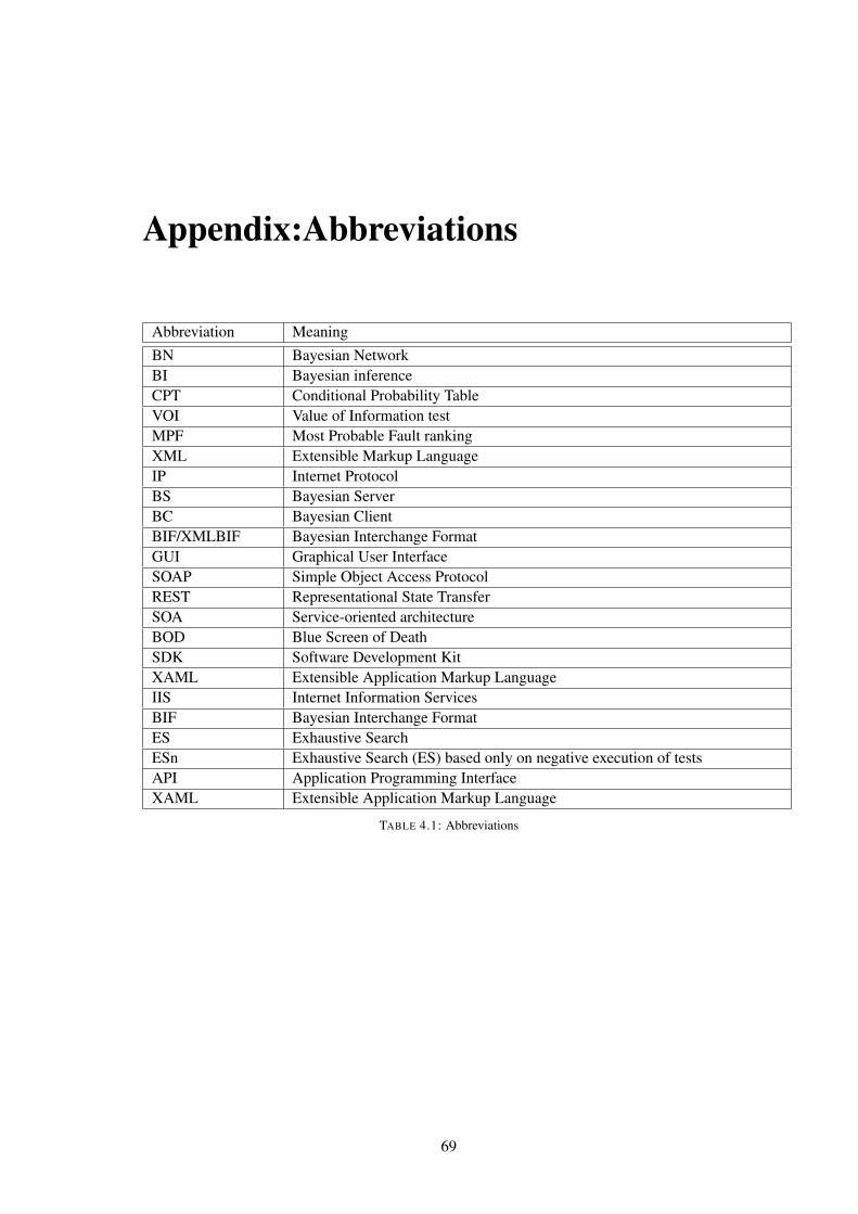
Appendix:Abbreviations

Abbreviation MeaningBN Bayesian NetworkBI Bayesian inferenceCPT Conditional Probability TableVOI Value of Information testMPF Most Probable Fault rankingXML Extensible Markup LanguageIP Internet ProtocolBS Bayesian ServerBC Bayesian ClientBIF/XMLBIF Bayesian Interchange FormatGUI Graphical User InterfaceSOAP Simple Object Access ProtocolREST Representational State TransferSOA Service-oriented architectureBOD Blue Screen of DeathSDK Software Development KitXAML Extensible Application Markup LanguageIIS Internet Information ServicesBIF Bayesian Interchange FormatES Exhaustive SearchESn Exhaustive Search (ES) based only on negative execution of testsAPI Application Programming InterfaceXAML Extensible Application Markup Language

TABLE 4.1: Abbreviations

69

Bibliography

[1] T. I. of Computer Science Poznan University of Technology. M3 - metrics, monitoring,

management, 2010. http://www.it-soa.pl/en/dymst/m3/index.html.

[2] A. Darwiche. What are bayesian networks and why are their applications growing across all

fields? Communications of the ACM, 53:80–90, December 2010.

[3] J. M. T. P. A. W. Bartosz Kosarzycki, Lukasz Rek. Service execution management in soa

systems. 2010.

[4] W. Feller and sons. An introduction to probability theory and its applications, 1960-1970.

[5] F. P. Miller. Conditional probability, December 2009.

[6] Marginal distribution, 2010. http://en.wikipedia.org/wiki/Marginal_

distribution.

[7] J. Jozefowska. Uncertainty modelling 2, bayesian networks, 2005.

[8] J. Elkink. Bayesian inference, October 14, 2008.

[9] E. L. Schreiber. d-separation, 1998.

[10] H. Bruyninckx. Bayesian probability. 2002.

[11] C. Hamalainen. Gibbs sampling, November 18, 2009.

[12] A. Panconesi. The stationary distribution of a markov chain, May 15, 2005.

[13] M. network. Making a service available across domain boundaries. http://msdn.

microsoft.com/en-us/library/cc197955(v=vs.95).aspx.

[14] F. G. Cozman. The interchange format for bayesian networks, 1998. http://www.poli.

usp.br/p/fabio.cozman/Research/InterchangeFormat/index.html.

[15] U. of Waikato. Weka 3: Data mining software in java. http://www.cs.waikato.ac.

nz/ml/weka/.

[16] U. o. P. Decision Systems Laboratory. The genie (graphical network interface) software

package, 2006.

[17] T. G. John Mark Agosta. Bayes network "smart" diagnostics. Intel Technology Journal,

08:361–372, November 17, 2004.

71

http://www.it-soa.pl/en/dymst/m3/index.html

http://en.wikipedia.org/wiki/Marginal_distribution

http://en.wikipedia.org/wiki/Marginal_distribution

http://msdn.microsoft.com/en-us/library/cc197955(v=vs.95).aspx

http://msdn.microsoft.com/en-us/library/cc197955(v=vs.95).aspx

http://www.poli.usp.br/p/fabio.cozman/Research/InterchangeFormat/index.html

http://www.poli.usp.br/p/fabio.cozman/Research/InterchangeFormat/index.html

http://www.cs.waikato.ac.nz/ml/weka/

http://www.cs.waikato.ac.nz/ml/weka/

Bibliography

[18] G. Casella and E. I. George. Explaining the gibbs sampler. The American Statistician, 46,

1995.

[19] C. Bishop. Introduction to bayesian inference, November 2, 2009.

[20] A. Nowak. Bayesian networks, probabilistic reasoning, genie, 1998.

72

© 2011 Bartosz Kosarzycki

Poznan University of TechnologyFaculty of Computing ScienceInstitute of Computing Science

Typeset using LATEX in Computer Modern.

BibTEX:@mastersthesis{ key,

author = "Bartosz Kosarzycki",title = "{Design and implementation of a computer systems diagnosis

tool using Bayesian networks}",school = "Poznan University of Technology",address = "Pozna{\’n}, Poland",year = "2011",

}

Documents

DESIGN AND IMPLEMENTATION OF A …sirius.cs.put.poznan.pl/...DiagnosisToolUsingBayesianNetworks.pdffor a specialised diagnosis service arose which would give the management system