1

ANALYSIS AND SIMULATION OF THE GEARSHIFT METHODOLOGY FOR

A NOVEL TWO-SPEED TRANSMISSION SYSTEM FOR ELECTRIC

POWERTRAINS WITH CENTRAL MOTOR

A. Sorniotti, T. Holdstock, G. Loro Pilone

University of Surrey

Guildford, Surrey GU2 7XH

United Kingdom

F. Viotto, S. Bertolotto

Oerlikon Graziano SpA

Via Cumiana 14

10098 Cascine Vica, Rivoli (TO)

Italy

M. Everitt, R. J. Barnes, B. Stubbs, M. Westby

Vocis Driveline Controls

American Barns

Banbury Road

Lighthorne, Warwick CV35 0AE

United Kingdom

2

Abstract

Electric vehicle powertrains traditionally consist of a central electric motor drive, a

single-speed transmission and a differential. This electric powertrain layout, either for

use in fully electric vehicles or through-the-road parallel hybrid electric vehicles, will be

extensively adopted in the next few years, despite the ongoing research in electric

vehicles with individually controlled motors. However, current research suggests that

electric powertrains with a central electric motor drive can still be widely improved. For

example, the installation of a seamless multiple-speed transmission instead of a single-

speed can provoke an increase in vehicle performance, together with an enhancement of

the overall efficiency of the electric powertrain. These novel transmission systems for

electric powertrains require a specific design, in order to be efficient, compact, easy and

robust to control, and cheap to manufacture. This article presents the mechanical layout

and the control system of a novel two-speed transmission system designed by the

authors, with particular focus on the achievement of optimal gearshift dynamics. The

torque characteristics of typical electric motor drives require a different actuation of the

seamless gearshifts, in comparison with the equivalent operation for a dual clutch

transmission within an internal combustion engine driven powertrain.

Keywords

2-speed transmission; seamless gearshift; control; electric powertrain

3

1. The Benefits of Multiple-Speed Transmission Systems for Electric Powertrains

Due to the nature of the torque characteristics of typical electric vehicle traction motors,

electric vehicles (or electric axles for through-the-road parallel hybrid electric vehicles)

are generally equipped with a single-speed transmission. This is due to electric motors

exhibiting a high constant torque from zero to base speed then entering into a constant

power region for higher angular velocities. A further benefit of a central motor drive

equipped with only a single-speed transmission is a reduction in the drivetrain mass,

volume, losses and cost [1-3].

Despite the wide operational speed range of such traction motors (e.g. from 0 to 8 000-

12 000 rpm), a multiple-speed transmission [4-6] may be employed to enhance the

vehicle performance. In particular the wheel torque at low vehicle velocities is increased

along with the maximum road gradient that the vehicle can ascend when transporting

heavy payloads. In addition, the lower second gear ratio raises the vehicle top speed.

As an example, Figure 1 shows the wheel torque envelops achievable through a single-

speed transmission in traction and regeneration, and the same characteristics for each

gear of a two-speed transmission system. The case study vehicle for Figures 1 and 2 is a

prototype electric minibus wherein the electric motor drive is characterised by a limited

regenerative capability due to the design of the power electronics. The two-speed

transmission brings an increase of approximately 34% of the peak value of wheel torque

over the single-speed axle, namely 800 Nm. Secondly, Figure 1 demonstrates the

4

benefit in vehicle top speed. At 0% of road gradient, the single-speed vehicle (in

unladen conditions) is characterised by a top speed VMax,SS,0% of 119 km/h, limited by

the maximum speed of the electric motor (8 000 rpm for the case study motor). The top

speed VMax,TS,0% for the two-speed vehicle is 149 km/h, limited by the available motor

power, but still showing a gain of 24% over the single-speed transmission vehicle.

Figure 1 – Potential performance benefit deriving from the adoption of a two-speed

transmission system over a single-speed for a case study vehicle

Moreover, in most cases the overall efficiency of the electric motor drive and energy

storage unit varies significantly as a function of the operating torque and speed. The

adoption of a two-speed transmission can facilitate significant energy benefits through

5

the optimisation of the operating points of the electric powertrain over a given driving

schedule. Consequently, the selection of the gear ratio is as important as in the case of a

conventional vehicle driven by an internal combustion engine. The efficiency of a

multiple-speed transmission system is generally lower than the efficiency of the single-

speed transmission for the same vehicle at least due to the losses relating to the presence

of an actuation system and increased mass. However this variation for conventional

transmission systems based on a layshaft layout, is usually marginal in comparison with

the potential increase in the overall powertrain efficiency. Evidence of this is

comprehensively provided in [4] and [7]. As an example, Figure 2 presents the

distribution of the operating points on the efficiency map of the electric motor drive

during a NEDC (New European Driving Cycle). The results are compared for the same

case study vehicle of Figure 1, equipped with a single-speed and a two-speed

transmission. The two-speed transmission system predominantly operates in second

gear at higher electric motor torques and lower speeds than the single-speed

transmission, and consequently in a higher efficiency region of the motor drive. This

conclusion is not only true for this singular case as the authors have derived diagrams

and results similar to those in Figures 1 and 2 for very different vehicle typologies and

electric powertrain characteristics [7].

6

Figure 2 – Potential energy efficiency benefit deriving from the adoption of a two-speed

transmission system

The existing literature suggests that two-speed transmission systems are the most

suitable solution for increasing the efficiency and performance of electric axles, [7-11],

without adding significant complexity and mass. [9] and [10] summarise the

optimisation procedures implemented for the choice of gear ratios and gearshift map for

two-speed transmission systems for electric axles. In particular, along a set of typical

driving schedules the energy consumption is reduced by approximately 10%, in

comparison with the single-speed vehicle equipped with the same motor drive and

energy storage unit. [11] adopts the same optimisation procedure of [9] and [10] in

7

order to demonstrate that a multiple-speed transmission system can permit a significant

reduction of the electric motor drive peak torque, for the same value of its peak power.

The downsizing (in peak torque) of the electric powertrain implies an additional benefit

in terms of mass, energy consumption and manufacturing cost.

This article presents the description of a novel transmission system layout specifically

designed for electric powertrains and the mathematical equations for modelling the

overall system dynamics. In addition, the principles of the methodology developed for

controlling the upshifts and downshifts with the new transmission are derived. The

issues which need to be addressed when designing a seamless gearshift control for

electric powertrains are discussed in great detail through a comprehensive set of

simulation results.

2. The Novel Transmission System

A multiple-speed transmission system must be able to accomplish seamless gearshifts in

order to be competitive against a single-speed transmission for electric axles. A

seamless gearshift is particularly relevant as a large number of upshifts (in conditions of

medium-high torque demands) are carried out in the constant power region of the

electric motor which can result in a perceivable torque gap.

Seamless gearshifts can be achieved by using a cascade of planetary gear sets, as

presented in [12], with a one-way clutch used to provide the torque reaction in first gear

8

during traction. A hydraulic actuation system is adopted for the control of the two

friction clutches required for the second gear, the reverse gear and regeneration. An

alternative seamless multiple-speed transmission layout for electric vehicle applications

can be based on the adoption of a Dual Clutch system on a layshaft type transmission,

as described in [13]. This solution is becoming common for internal combustion engine

driven vehicles, but is characterised by a significant mechanical complexity and requires

careful control of the actuation of the on-going and off-going friction clutches [14]. As a

consequence, this layout is suitable for transmission systems characterised by at least

three gear ratios, but more cost-effective solutions can be evaluated for seamless two-

speed transmissions for electric vehicles. In particular, according to [15] and [16], the

use of one-way clutches can improve shift quality to a great extent, as their ability to

automatically disengage if the input torque becomes negative benefits the control of a

clutch-to-clutch gearshift. An alternative design solution for the implementation of

seamless gearshifts is based on a novel design of the synchronising rings and their

actuation [17].

The novel two-speed transmission system of this paper combines the mechanical

simplicity of a layshaft type transmission, with the high quality of a clutch-to-clutch

gearshift. Its primary components are a one-way sprag clutch located on the secondary

shaft and a friction clutch on the primary shaft along with an open differential, as

displayed in Figure 3. The input torque is transmitted by the sprag clutch whilst in first

9

gear, and by the friction clutch whilst in second gear. The system can work either as a

fully automated transmission, or as an automated manual transmission through a

seamless shift system [18]. The friction clutch is applied to transfer torque from the

sprag clutch during an upshift, and released to allow the sprag clutch to engage to

accomplish a downshift. A full description of the gearshift methodology is presented in

section 4.

Figure 3 – Schematic of the transmission operation in first gear (left) and second gear

(right)

The multi-disc friction clutch utilises sintered metal friction material and is electro-

hydraulically controlled using a remote brushless motor driven actuator, pressurising a

master cylinder mechanically connected to the Belleville spring of the friction clutch.

The friction clutch actuation system is controlled through a feedback loop based on

actuator displacement. In order to allow regenerative energy recovery whilst

10

decelerating in first gear, the engagement of a locking ring, electro-mechanically

actuated, prevents the one-way sprag clutch from overrunning when the direction of

torque through the transmission is reversed. Once the vehicle has come to rest, the

gearshift mechanism can also be used as a park lock by simultaneously engaging the

locking ring and closing the friction clutch, thus eliminating the need for a separate park

lock mechanism and actuator. The mechanical layout of the two-speed transmission

results in a compact design, with the overall distance between the primary and

differential shaft being about 200 mm for a premium passenger car. Furthermore, for

this application the distance from the primary shaft to the secondary shaft is less than

110 mm and secondary shaft to the differential is approximately 125 mm. The

transmission with this layout results in a mass of about 38 kg. The dimensions and

weight are comparable with the single-speed unit (25 kg) from which this novel

transmission was derived.

3. Transmission Dynamics: Governing Principles

The best methodology for developing the control system for the gearshift actuation is

through the analysis of the equations governing the overall system dynamics [19].

Starting from the basic physical principles described in this section, the control system

for the gearshift actuation will be described in detail in section 4.

11

The derivation of the equations governing the dynamics of the bespoke two-speed

transmission system has been carried out in [20], therefore only the final dynamic

equations are presented here. In the following description of the first order system

dynamics the plays and internal torsion deformations of the transmission components,

in particular of the engaged sprag clutch, are not considered as they are second

approximation effects in relation to the gearshift control analysis which is the focus of

the article. In fact, these characteristics do not affect the acceleration profile of the

vehicle in conditions of constant gear or upshift / downshift. Experimental tests on the

sprag clutch have revealed that its internal elastic deformation, proportional to the

transmitted torque (with a maximum torsion angle of 2-3 deg), is negligible in

comparison with the torsion dynamics of the half-shafts, from the viewpoint of the

vehicle low frequency drivability.

The transmission system can work in three different states, each of which is

characterised by different governing equations:

Engaged first gear. In this condition the kinematical ratio between the electric

motor shaft speed and the transmission output shaft speed is equal to the first

gear ratio, and the friction clutch can be transmitting torque while slipping

during a gearshift (torque phase of the gearshift).

Inertia phase of the gearshift. In this condition both clutches are slipping, and

the transmission system is characterised by two degrees of freedom, as the

12

electric motor dynamics are decoupled from the transmission output shaft

dynamics.

Engaged second gear. In this condition the friction clutch is engaged and no

torque is transmitted through the sprag clutch, which is overrunning.

3.1 Engaged First Gear

Equation (3.1) governs the overall transmission dynamics in this condition, derived

through each shaft moment balance equation:

1 1 2 2 1 1

, , 1

m diff diff h fc diff diff fc diff diff

diff

eq trans gear

T i η i η T T i η i η T i η i ηθ

J

(3.1)

The efficiencies in the formulas (the η terms, having values between 0 and 1) can be

reversed depending on the direction of the transmitted power through the coupling.

With reference to the differential, the equivalent moment of inertia of the transmission

in first gear is given by:

2 2

, , 1 1 1 1

2 2 2

1 2 2 2 2

0.5 0.5eq trans gear diff LHS RHS m diff diff

b diff diff b diff diff

J J J J J J i η i η

J i η i η J J i η

(3.2)

During normal operation of the first gear, Tfc = 0, but throughout the torque phase of the

gearshift, the friction clutch is transmitting increasing (in case of upshift) or decreasing

(in case of downshift) torque Tfc while slipping. When the friction clutch torque is

applied, the system experiences a torque variation at the differential due to the term

13

Tfc·idiff··ηdiff· (i2·η2-i1·η1) in the numerator of equation (3.1), as part of the transmission

input torque is transmitted to the output shaft of the transmission through gear one

(torque contribution (Tm-Tfc)·i1·η1·idiff·ηdiff), and part through gear two (torque

contribution Tfc·i2·η2idiff·ηdiff). If the locking ring is disengaged, the system still operates

in first gear if the sprag clutch torque Tsc is positive (i.e. the system is in traction).

3.2 Inertia Phase of the Gearshift

During the inertia phase of the gearshift, the ratio between motor speed and output shaft

speed is intermediate between i2 and i1. In such a condition, the equation describing

motor dynamics is:

212

1 1

m fc

mb

m

T Tθ

JJ J

i η

(3.3)

whilst the equation for transmission dynamics is:

2 2

, ,

fc diff diff h

diff

eq trans IP

T i η i η Tθ

J

(3.4)

where:

2 2 2

, , 1 2 2 20.5 0.5eq trans IP diff LHS RHS b diff diff diff diffJ J J J J i η i η J i η (3.5)

The equivalent moment of inertia of the transmission system in this condition is much

lower than in equation (3.2), mainly because equation (3.4) does not include the electric

motor inertia. This makes the first natural frequency of the transmission during the

14

inertia phase of the gearshift much higher than when the system works either in first or

second gear, Figure 4. The high natural frequency can result in possible dynamic and

NVH (Noise, Vibration and Harshness) problems in case of a non-optimal tuning of the

friction clutch and its control.

3.3 Engaged Second Gear

In second gear, the overall transmission is characterised by one degree of freedom, as in

first gear. The transmission system dynamics in second gear are governed by:

2 2

, , 2

m diff diff h

diff

eq trans gear

T i η i η Tθ

J

(3.6)

Equation (3.7) is the expression of the equivalent moment of inertia of the transmission

in second gear:

, , 2

2 2

2 2 22 2 2

1 1 2 2 22

1 1

0.5 0.5eq trans gear diff LHS RHS

b diff diff

m b diff diff diff diff

J J J J

J i η i ηJ J J i η i η J i η

i η

(3.7)

The equivalent moment of inertia described by equation (3.7) is lower than the one of

equation (3.2), predominantly due to the fact that the moment of inertia of the electric

motor drive is multiplied by i22 instead of i1

2.

3.4 System Dynamics in the Frequency Domain

Figure 4 illustrates the overall system dynamics in the three states described in sections

15

3.1-3.3, considering the overall half-shaft torque as an output with the inputs being the

reference electric motor drive torque when the gears are engaged, or the friction clutch

torque during the inertia phase. These Bode diagrams have been obtained from a

linearised model of the overall system, including the dynamics of the electric motor

drive, friction clutch actuation system and tyre slip, the tyre relaxation length and half-

shaft compliance.

Figure 4 – Frequency response of the system in first gear, second gear and during the

inertia phase for system linearization at 10 m/s of vehicle speed

The variation of the first natural frequency of the driveline is evident from first to

second gear due the lower value of the equivalent moment of inertia (at the wheels) of

16

the electric motor. The natural frequency is subjected to a further significant increase

during the inertia phase, as the equivalent moment of inertia of the drivetrain is reduced

when the electric motor is decoupled from the wheels. The amplitude of the frequency

response is reduced between 1 and 25 Hz during the inertia phase, due to the dynamic

characteristics (time constant) of the friction clutch actuator.

4. The Gearshift Control System

4.1 Upshift Control

The control of the upshifts for such a transmission system is similar to the methodology

usually adopted for dual clutch transmission systems, with some differences to

compensate for the characteristics of the electric powertrain. In this section, upshifts

during power-on are analysed.

In order to shift to second gear, firstly the locking ring is disengaged. The torque phase

is then initiated by the progressive engagement of the friction clutch at a rate limited by

the dynamic properties (reaction time and rise time) of the electro-hydraulic actuation

system. This provokes a reduction of the torque Tsc transmitted through the sprag clutch

while the system is kinematically in first gear and consequently changes the

transmission output torque from the first to the second gear value. The progressive

transition reduces the drivetrain oscillations which can be observed in a conventional

manual transmission system, where the disengagement of the clutch typically provokes

17

an interruption of the half-shaft torque and produces the consequent excitation of the

torsional dynamics of the system. The basic version of the control system presented in

this paper, called ‘Control 1’, does not manipulate the driver torque demand, which is

directly sent to the motor drive, during the torque phase of the upshift.

At the end of the torque phase the sprag clutch torque Tsc becomes null for the friction

clutch torque value identified by the following equation:

2

, 1

1 1

b diff diff

fc dis m m m

J θ iT T J J θ

i η

(4.1)

Tfc is estimated by the control system from the displacement of the friction clutch

actuator. Equation (4.1) establishes the beginning of the inertia phase of the upshift,

during which the electric motor speed has to be reduced from the value for the first gear

ratio to the value for the second gear ratio, whilst keeping an adequate vehicle

acceleration profile. The principles for the inertia phase control can be derived from

equations (3.3) and (3.4). During the inertia phase, vehicle acceleration dynamics are

controlled by the friction clutch torque (equation (3.4)), whilst the difference between

electric motor torque and friction clutch torque affects the motor dynamics (equation

(3.3)). As a consequence, the two degrees of freedom of the system can be

independently controlled, provided that the electric motor drive is not working in

conditions of saturation (on its peak torque characteristic, which represents the

18

constraint of the control system). This is the ‘golden rule’ for the control of the inertia

phase of the gearshifts in such a system.

During the inertia phase of the upshift for ‘Control 1’, Tfc is ramped up according to an

open-loop control system at the same rate as the torque phase to reduce any driveline

oscillations during phase transitions. Tfc ramps to a reference level equal to the torque

value the electric motor would produce for the actual condition of driver torque demand

DTD(t) (not manipulated by the controller) and electric motor speed. Additional terms

compensate for the inertial torque of the main components of the system. Tfc,saturation,IP,US

is given by:

, , , 1,fc saturation IP US m m m mT t T DTD t θ t J J θ (4.2)

In the meantime, electric motor dynamics are controlled by the combination of a

feedforward and a feedback (Proportional Integral Derivative - PID) controller (Figure

5), based on a reference speed profile equal to:

)(1, IPdiffdiffrefm tyii (4.3)

where the adimensional factor y(tIP) is a normalisation parameter defining the reference

speed profile, according to the qualitative shape in Figure 5. tIP is the output of a counter

which is activated by the transmission control unit at the beginning of the inertia phase.

The initial value of y is 1, so that equation (4.3) provides an initial value of the reference

motor speed equal to the actual speed of the unit at the beginning of the upshift. The

19

final value of y is equal to the step ratio i2/i1, so that the final value of the reference

motor speed is equal to the one required for the synchronization of the friction clutch.

Figure 5 – Block diagram of the feedforward / feedback control system of electric motor

speed during the inertia phase of the upshift

The shape of y(tIP) is designed so that the electric motor reference speed is at a

maximum in the first part of the inertia phase, and reduces to zero (for the specific

tuning shown in Figure 5) at the time tIP,end at the end of the inertia phase. The shape of

the profile can be tuned to alter the duration of the inertia phase, depending on the

vehicle parameters and required upshift performance, and the amount of perceived

discontinuity at the engagement point of the friction clutch at tIP,end. If the air-gap

torque dynamics of the motor drive is modelled through a first order transfer function,

IPt

Feedforward

,m refT

+

y

P

I

DtIP

i2/i1

1

0 tIP,end

+

tm

1iidiffdiff

estfcT ,

DTD

m

IPdiffdiffrefm tyii 1,

20

the open-loop transfer function of the feedback part of the controller of Figure 4 is given

by:

mm

IDP

mrefm

m

ssJs

KsKK

ss

s

1

1

,

(4.4)

Hence the gains of the feedback part of the controller can be tuned according to the well

known rules in terms of tracking capability (bandwidth) and phase margin [21].

Figure 6 – Bode diagram of the open-loop and closed-loop transfer functions for the

feedback part of the electric motor control loop

Figure 6 shows an example of possible tuning of the PID control parameters and the

relating open-loop (given by equation (4.4)) and closed-loop transfer functions. The

transfer functions are affected by the time constant m of the electric motor air-gap

21

torque dynamics (sometimes filtered for anti-jerk purposes). Consequently a sensitivity

analysis has been added to Figure 6 to illustrate the effect of the motor time constant.

The parameters of the electric motor controller can vary depending on DTD and speed,

in order to make the upshift quicker or more comfortable as a function of the specific

driving situation. In any case, the motor controller has very low impact on the low

frequency vehicle drivability during the upshift, as this is controlled through the friction

clutch (equation (4.2)), consistently with the ‘golden rule’. Therefore, the performance

of the system is very robust against the variation of the parameters of the feedback

motor controller. Tests have been successfully carried out with only the feedforward

system reducing the electric motor drive torque by a constant amount and so with no

contribution from the PID, with little variation of the perceivable quality of the achieved

results.

At the conclusion of the inertia phase, when the friction clutch engages, the friction

clutch actuator is moved to its endstop where the transmissible clutch torque is at the

nominal level, depending on the wear condition of the clutch disks.

22

Figure 7 – Possible conditions of an upshift manoeuvre on the electric motor drive

torque characteristic, under the hypothesis of constant driver torque demand DTD

during the manoeuvre

The upshift control system described until now (‘Control 1’) gives origin to a complete

absence of torque gap during the upshift when the initial and the final operating points

of the electric motor drive are in the constant torque region of the electric motor. For

example, this condition is satisfied for the upshifts from point A to B or point C to D in

Figure 7. For upshifts in the constant power region of the electric motor drive, such as

those from E to F or G to H, the torque phase of the upshift, when operated as described

for ‘Control 1’, involves a reduction of wheel torque. For the same conditions, the

inertia phase implies a progressive increase of wheel torque, consistent with the

reduction of electric motor speed and the subsequent increase of Tfc,saturation,IP,US

A B

C D

F

E

H

G

Tm

mθ

baseθ

23

(equation (4.2)). These variations of wheel torque, especially the increase during the

inertia phase, are progressive and provoke lower jerk (time derivative of vehicle

acceleration) levels and significantly better acceleration profiles than those experienced

in a conventional single-clutch transmission, which would provoke negative values of

vehicle acceleration during the phase of the upshift characterised by the disengaged

clutch. The control system defined as ‘Control 1’ is reliable, robust and relatively

simple; therefore it is currently adopted on the first transmission prototypes mounted

onto an electric minibus demonstrator and on the Hardware-In-the-Loop electric axle rig

at the University of Surrey.

In order to significantly reduce the torque gap during the inertia phase of the upshift, it

is possible to adopt the following control characteristic, here named ‘Control 2’, for the

friction clutch saturation level:

, , , , 2 2 1,fc saturation IP US C m diff diff m mT t T DTD t θ t i i J J θ (4.5)

The control system provokes the friction clutch to transmit a torque level equal to the

value the electric motor would generate if the system was already in second gear. The

adoption of the friction clutch torque of equation (4.5) during the inertia phase of the

upshift significantly improves vehicle acceleration, as it eliminates the partial wheel

torque gap during the inertia phase of the upshift. However, it generates significant

vehicle jerk in the transition between the torque phase and the inertia phase of the

upshift. This is due to the fact that the torque phase of the upshift, when implemented

24

according to ‘Control 1’ and ‘Control 2’, intrinsically produces a reduction of the

available wheel torque which is progressively recovered in case of ‘Control 1’ but quite

abruptly recovered in case of ‘Control 2’. ‘Control 2’ could be adopted as a sport-

oriented transmission control algorithm selectable by the driver.

In the case of an upshift in the constant power region of the electric motor, it is possible

to compensate for the reduction of wheel torque, induced by the torque shift from the

first to the second gear (torque phase of the upshift), by manipulating the electric motor

torque demand. This variant of the control system is defined as ‘Control 3’ and is

described by equation (4.6):

2, , , , 3 ,

1

( , ) 1m ref TP US C m m fc est

iT t T DTD θ T

i

(4.6)

With the implementation of such a control system during the entire torque phase, the

disengagement of the sprag clutch would happen at a friction clutch torque level equal

to:

2 1, 1

1 1 2

( , )b diff diff

fc dis m m m m

J θ i iT T DTD θ J J θ

i η i

(4.7)

As a consequence, the final level of the friction clutch torque during the torque phase of

the upshift could be higher than the desired friction clutch torque of equation (4.5) for

the inertia phase of the upshift, which is the same for ‘Control 2’ and ‘Control 3’, in

case of an upshift carried out in the constant torque region of the electric motor drive. In

25

order to prevent a significant negative jerk (due to the reduction of the friction clutch

torque) at the transition between the torque phase and the inertia phase of the upshift,

when Tfc,est> Tfc,saturation,IP,US,C2, Tm,ref,TP,US,C3 is switched back to the level imposed by the

driver torque demand DTD(t). During this transition careful tuning of the control

parameters have to be carried out, paying particular attention to the dynamics of the

friction clutch actuator and the electric motor. The system sensitivity to the clutch

actuator dynamics has already been demonstrated in [20].

4.2 Downshift Control

As a first approximation, the downshift actuation sequence is a reverse of the upshift

method, wherein the inertia phase precedes the torque phase. Downshifts in power-on

are actuated following significant increases of driver torque demand DTD, in order to

increase the amount of wheel torque. Due to the significantly lower frequency of

downshifts in power-on in comparison with the upshifts (consequence of the usual gear

selection algorithms), the control system adopted in the inertia phase is a simplified

version of the one presented for the upshifts, even if potentially the control systems

could be similar.

Downshifts in power-on are accomplished by initially opening the friction clutch at the

rate allowed by the actuator dynamics. When the clutch transmissible torque is lower

than the electric motor torque, the clutch starts slipping, giving origin to the inertia

26

phase. The motor torque is kept at the level requested by the user, whilst the friction

clutch torque is controlled in order to produce the required acceleration level of the

electric motor shaft. At the start of the inertia phase, the friction clutch actuator position

should be carefully monitored due to the dynamic friction coefficient of the dry friction

clutch being lower than the static friction coefficient. The manipulation of both motor

torque and friction clutch torque (according to the ‘golden rule’ presented in section 4.1)

during the inertia phase of the downshift in power-on would lead to the full

controllability of both electric motor dynamics and vehicle acceleration, at the cost of a

significantly increased complexity of the control system and the time required to tune its

parameters for each vehicle application. The friction clutch can be momentarily re-

engaged when the sprag clutch is about to connect (beginning of the torque phase of the

downshift), in order to dampen the re-engagement of the sprag clutch and reduce any

jerk.

5. Results

A non-linear vehicle simulation model has been implemented in order to evaluate the

gearshift dynamics of the novel transmission system. The equations utilised to model

the transmission dynamics have been presented in section 3.

The developed simulator is characterised by a detailed transmission efficiency model,

based on the efficiency maps for the transmission and the final reduction ratio

27

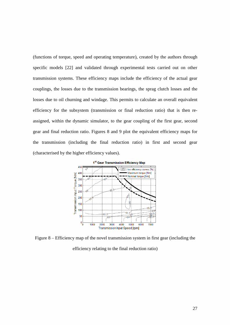
(functions of torque, speed and operating temperature), created by the authors through

specific models [22] and validated through experimental tests carried out on other

transmission systems. These efficiency maps include the efficiency of the actual gear

couplings, the losses due to the transmission bearings, the sprag clutch losses and the

losses due to oil churning and windage. This permits to calculate an overall equivalent

efficiency for the subsystem (transmission or final reduction ratio) that is then re-

assigned, within the dynamic simulator, to the gear coupling of the first gear, second

gear and final reduction ratio. Figures 8 and 9 plot the equivalent efficiency maps for

the transmission (including the final reduction ratio) in first and second gear

(characterised by the higher efficiency values).

Figure 8 – Efficiency map of the novel transmission system in first gear (including the

efficiency relating to the final reduction ratio)

28

Figure 9 – Efficiency map of the novel transmission system in second gear (including

the efficiency relating to the final reduction ratio)

The simulation model includes the estimation of the temperature dynamics of the

electric powertrain components (air cooled transmission), and in particular the thermal

dissipation within the friction clutch during the gearshifts, which are fed into the

efficiency model. The model also considers the wear in the system and the play in the

actuation of the clutch, evident in the delay between the motion of the pressure plate and

the actual torque on the friction clutch. The transmission model includes the torsional

dynamics of the half-shafts; the tyres are modelled using Pacejka’s magic formula [23]

with tyre relaxation length. The adopted vehicle dynamics simulator permits the

detailed modelling of vehicle longitudinal dynamics and has already been

experimentally validated by the authors on electric vehicle applications equipped with

29

single-speed transmission systems [7]. The main vehicle parameters adopted for the

simulation results of Figures 10 to 15 are listed in Table A.1. The motor drive data was

selected to have a high moment of inertia and slow reaction time to test the robustness

of the proposed controllers in critical conditions.

5.1 Upshift

Figures 10 and 11 summarise the overall transmission system dynamics for an upshift at

80% of driver torque demand, carried out at a vehicle speed of 75 kph, in the constant

power region of the electric motor drive and using control system ‘Control 3’.

30

Figure 10 – Electric motor drive dynamics and gear input torques during an upshift at

80% of driver torque demand

The phases of the upshift, namely ‘Upshift Request’ followed by the torque phase,

inertia phase (defined by ‘Inertia Phase Start’ and ‘Inertia Phase End’) and the final

motion of the actuator after the engagement of the second gear (defined by ‘Actuator

Stop’), are evident in the graphs. The effect of the efficiencies and the moments of

inertia of the components are also visible in the graphs, for example in the marginal

difference between the electric motor torque and the input torques transmitted by gear

one and two when a gear is engaged in Figure 10.

Torque Phase

31

Figure 11 – Clutch dynamics during an upshift at 80% of driver torque demand

During the torque phase the electric motor torque demand is modified according to

equation (4.6) and is increased in order to compensate for the reduction of vehicle

acceleration induced by the torque transfer from first to second gear. Due to the sharp

gradient in the reference electric motor speed at the start of the inertia phase, the

feedforward and feedback controller shown in Figure 5 provokes a large decrease in

electric motor torque (Figure 10). The friction clutch torque is ramped up to make the

vehicle acceleration equal to the level of the vehicle acceleration in second gear,

according to equation (4.5). In the second part of the inertia phase the rate of motor

reference speed is reduced as shown in the graph of Figure 5, and consequently the

32

electric motor torque demand is increased. Moreover as the electric motor speed

reduces, the maximum available torque increases due to the torque map of the electric

motor (Figure 7). This justifies the difference between the first gear torque and the

second gear torque in conditions of engaged gear in Figure 10, and represents the main

peculiarity to be taken into account in the implementation of algorithms for gearshift

control of electric powertrains.

The torque actually transmitted by the friction clutch and the maximum torque which

can be potentially transmitted (transmissible torque) for an assigned clutch actuator

displacement are the same when the clutch is slipping, as in Figure 11, whilst they differ

when the clutch is enganged. This is evident after the inertia phase, when the

transmissible torque of the friction clutch is increased due to the change between the

dynamic and static friction coefficient of the clutch. Finally the actuator is moved to

increase the friction clutch axial force and therefore the transmissible torque. Notably,

Figure 11 shows that the friction clutch torque transmitted in second gear is lower than

that transmitted by the sprag clutch in first gear due to the friction clutch being located

on the primary shaft whilst the sprag clutch is located on the secondary shaft as

illustrated in Figure 3.

In addition, Figure 11 illustrates that the pressure plate moves when the shift is initated

to take up any play between the clutch plates. After recovering the play, during the

torque and inertia phases of the upshift there is an infinitesimal axial movement of the

33

pressure plate due to the high axial stiffness of the clutch plates, athough the

transmissible torque varies with the friction clutch actuator travel, which depends on the

sitffness properties of the Belleville spring.

Figure 12 – Half-shaft torque dynamics during the same upshift of Figures 10 and 11

(constant power region of the electric motor), and during an upshift at 40% of driver

torque demand and 30 kph (constant torque region of the electric motor)

Figure 12 plots the time history of half-shaft torques (sum of the torques of the left and

right half-shafts) for the same manoeuvre as in Figures 10 and 11, and during an upshift

at 40% of driver torque demand, carried out at 30 kph, in the constant torque region of

34

the electric motor drive. Both manoeuvres have been simulated by adopting ‘Control 3’.

The marginal torque gap induced by the torque phase of the upshift and recovered by

the friction clutch control during the inertia phase is evident in the first manoeuvre. The

second manoeuvre is characterised by the total absence of any torque gap. This

characteristic is common to ‘Control 1’, ‘Control 2’ and ‘Control 3’, when the upshift is

requested in the constant torque region of the electric motor unit. The equivalent

moment of inertia of the transmission is very high in first gear and very low during the

inertia phase and it is this change which provokes some marginal oscillations in the

half-shaft torque.

Figure 13 compares the vehicle acceleration profiles achievable during two different

upshifts at 40% (different manoeuvre from Figure 12) and 80% (identical manoeuvre to

Figures 10 to 12) of driver torque demand, both in the constant power region of the

electric motor drive. Table 3 provides an objective comparison of the three gearshift

strategies during each manoeuvre.

35

Figure 13 – Upshifts in the constant power region of the electric motor drive, at 40%

(different from the upshift in Figures 7-9) and 80% (the same as in Figures 7–9) of

driver torque demand: vehicle acceleration profiles achievable with ‘Control 1’,

‘Control 2’ and ‘Control 3’

Table 1 – Comparison of ‘Control 1’, ‘Control 2’ and ‘Control 3’ during the same

upshift manoeuvres of Figure 13 (in the constant power region)

Torque Demand 40 – 100

km/h

70 – 100

km/h

Upshift

time

Mean

acceleration

during upshift

Mean jerk

during

upshift

40% Control 1 14.91 s 9.55 s 1.11 s 0.76 m/s

2 0.95 m/s

3

Control 2 14.71 s 9.34 s 1.35 s 1.00 m/s2 1.18 m/s

3

Control 3 14.68 s 9.32 s 1.39 s 1.01 m/s2 0.41 m/s

3

80% Control 1 6.53 s 4.03 s 0.95 s 1.82 m/s

2 2.24 m/s

3

Control 2 6.33 s 3.84 s 0.70 s 2.25 m/s2 3.22 m/s

3

Control 3 6.31 s 3.82 s 0.74 s 2.31 m/s2 2.15 m/s

3

36

‘Control 2’ shows most of the benefit from the viewpoint of the acceleration time (a

gain of more than 0.2 s when compared to ‘Control 1’), however the mean of the

absolute value of jerk (time derivative of vehicle acceleration) during the simulation of

the upshift is higher than for ‘Control 1’, with an even more significant disadvantage in

terms of peak value of jerk. ‘Control 3’ represents the best compromise between a high

performance upshift and the requirement for the expected comfort level. At 80% of

torque demand, the benefit of ‘Control 3’ is much more limited than at 40% of torque

demand, due to the fact that the torque increase specified by ‘Control 3’ is saturated at

the peak torque of the electric motor (at 100% of motor torque demand, ‘Control 3’

produces the same performance as ‘Control 2’).

5.2 Downshift

Figure 14 summarises the torque and speed dynamics for a power-on downshift (kick-

down) during a tip-in test (a sudden driver torque demand request) from 25 kph where

the final driver torque demand is 80%. The downshift takes place in the constant torque

region of the electric motor, and so is performed to provoke an increase in available

wheel torque. Figure 14 illustrates the oscillations (circled) in the speeds due to the

effect of the tip-in manouvre on the torsional dynamics of the half-shafts. The

transmitted second gear torque reduces at the start of the inertia phase due to the change

in the friction coefficient from the static to the dynamic value. This is also evident in

37

Figure 15 which shows that the change is partially compensated by the motion of the

friction clutch actuator. At the end of the inertia phase, when the motor speed is at the

required level and the sprag clutch is engaged, the friction clutch torque is progressively

reduced to zero during the torque phase.

Figure 14 – Speed and torque dynamics during a downshift in power-on for a tip in test

at an intial speed of 25 kph and a final 80% driver torque demand

Tip-in and kick-down

38

Figure 15 – Clutch dynamics during a downshift in power-on for a tip in test at an intial

speed of 25 kph and a 80% driver torque demand

6. Conclusion

Multiple-speed transmissions for electric powertrains with a central electric motor give

rise to significant performance and energy efficiency benefits in comparison with

conventional single-speed transmissions. Specifically a two-speed transmission system

represents the best compromise between the advantages of a multiple-speed

transmission system and the simplicity of a compact and lightweight drivetrain. This

article has presented a novel two-speed transmission system design, together with the

equations governing its dynamics. Three alternative gearshift control systems have been

outlined, with particular reference to the typical characteristics of electric powertrains,

39

which require novel control algorithms for a seamless management of the upshifts

within the constant power region of the electric motor drive. A comprehensive set of

simulation results has demonstrated the functionality of the implemented control system

and mechanical hardware, currently under experimental testing.

7. References

1. Ehsani, M., Gao, Y., Emadi, A., Modern Electric, Hybrid Electric, and Fuel Cell

Vehicles, 2nd

Edition, Routledge, 2009.

2. Husani, I., Electric and Hybrid Vehicles, CRC Press, 2003.

3. Miller, J. M., Propulsion Systems for Hybrid Vehicles, Ed. IEEE, 2004.

4. Ren, Q., Crolla, D.A., Morris, A., Effect of Transmission Design on Electric

Vehicle (EV) Performance IEEE Vehicle Power and Propulsion Conference, 7-10

September 2009.

5. Turner, A., Cavallino, C., Multi-Speed EV/FCV Transmission with Seamless

Gearshift, 2009 CTI Conference, Berlin.

6. Knodel, U., Electric Axle Drives for Axle-Split-Hybrids and EV-Applications, 9th

European All-Wheel Drive Congress, Graz, 2009.

7. Sorniotti, A., Subramanyan, S., Cavallino, C., Viotto, F., Bertolotto, S., Turner,

A., Selection of the Optimal Gearbox Layout for an Electric Vehicle, SAE 2011 World

Congress, Cobo Center, Detroit, 12-14 April 2011, SAE 2011-01-0946.

40

8. Eberleh, B., Hartkopf, T., A high speed induction machine with two-speed

transmission as drive for electric vehicles, IEEE International Symposium on Power

Electronics, Electrical Drives, Automation and Motion, Taormina, 23-26 May 2006.

9. Sorniotti, A., Boscolo, M., Turner, A., Cavallino, C., Optimisation of a 2-speed

Gearbox for an Electric Axle, AVEC 10, University of Loughborough, 22-26 August

2010, paper 229.

10. Sorniotti, A., Boscolo, M., Turner, A., Cavallino, C., Optimisation of a Multi-

Speed Electric Axle as a Function of the Electric Motor Properties, IEEE VPPC 2010,

Lille, 1-3 September 2010, VPPC.2010.5729120.

11. Di Nicola, F., Optimisation of the Gearbox for a Fully Electric Passenger Car, MSc

Thesis, Politecnico di Torino, October 2010.

12. Koneda, P.T., Stockton, T.R., Design of a Two-Speed Automatic Transaxle for an

Electric Vehicle, SAE 1985 World Congress, 1 February 1985, SAE 850198.

13. Webster, H., A Fully Automatic Vehicle Transmission Using a Layshaft Type

Gearbox, SAE 1981 World Congress, 1 February 1981, SAE 810104.

14. Kulkarni, M., Shim, T., Zhang, Y., Shift dynamics and control of dual-clutch

transmissions, Mechanism and Machine Theory 42, 2007, pp. 168-182.

15. Goetz, M., Levesley, M. C., Crolla, D. A., Integrated Powertrain Control of

Gearshifts on Twin Clutch Transmissions, 8 March 2004, SAE 2004-01-1637.

41

16. Goetz, M., Levesley, M.C., Crolla, D.A., Dynamics and control of gearshifts on

twin-clutch transmissions, Proceedings of the Institution of Mechanical Engineers, Part

D: Journal of Automobile Engineering, Vol. 219, 2005, pp. 951-963.

17. Heath, R.P.G., Child, A. J., Zeroshift. A seamless Automated Manual

Transmission (AMT) with no torque interrupt, SAE 2007 World Congress, 16 April

2007, SAE 2007-01-1307.

18. Oerlikon Graziano S. p. A., Cavallino, C., Trasmissione a due marce per veicoli

elettrici, Italian Patent TO2009A000750, 2009.

19. Zheng, Q., Srinavasan, K., Rizzoni, G., Transmission shift controller design based

on a dynamic model of transmission response, Control Engineering Practice, Vol. 7,

Issue 8, August 1999, pp. 1007-1014.

20. Sorniotti, A., Loro Pilone, G., Viotto, F., Bertolotto, S., Barnes, R. J., Morrish,

I., Everitt, M., A Novel Seamless 2-Speed Transmission System for Electric Vehicles:

Principles and Simulation Results, SAE TO ZEV Conference, 9-10 June 2011, SAE

2011-37-0022.

21. Ogata, K. Modern Control Engineering, Prentice Hall, 5th

edition, 2009.

22. Cavallino, C., Torrelli, C., Viotto, F., Efficiency of a Wet DCT for a High

Performance Vehicle: Sensitivity Analysis and Measurements, oral presentation, SAE

2009 Conference: Facing the Challenges of Future CO2 Targets, Turin (Italy), 18-19

June 2009.

42

23. Pacejka, H.B., Tyre and Vehicle Dynamics, 2nd

Edition, Ed. Butterworth-

Heinemann, 2005.

Appendix A – Main Vehicle Parameters

The simulation results presented in Figures 10-15 refer to a front-wheel-drive vehicle

characterised by the following parameters.

Unit Value

m [kg] 1785

Mass Distribution [%front/%rear] 52/48

L [m] 2.80

RW [m] 0.34

Tm,MAX [Nm] 450

nm,base [rpm] 3400

i1 [-] 3.12

i2 [-] 1.74

idiff [-] 3.00

Jmot [kgm2] 0.18

τm [ms] 120

τFC [ms] 70

kL,HS [Nm/rad] 8500

kR,HS [Nm/rad] 11700

Table A.1 – List of the main vehicle and transmission parameters

43

Appendix B – List of Notations

DTD: driver torque demand (equivalent to the throttle command for a conventional

internal combustion engine driven vehicle)

idiff: final reduction ratio

i1: first gear ratio

i2: second gear ratio

nbase: electric motor base speed

Jdiff: equivalent moment of inertia of the differential

Jeq,trans,gear1: equivalent moment of inertia (at the differential) of the transmission in first

gear

Jeq,trans,gear2: equivalent moment of inertia (at the differential) of the transmission in

second gear

Jeq,trans,IP: equivalent moment of inertia (at the differential) of the transmission during

the inertia phase

JLHS: moment of inertia of the left half-shaft

Jmot: moment of the electric motor

JRHS: moment of inertia of the right half-shaft

J1: moment of inertia of the input shaft of the transmission (primary shaft), as indicated

in Figure 3

44

J1b: moment of inertia of the part of the friction clutch (located on the transmission input

shaft) gearing with the secondary shaft of the transmission, as indicated in Figure 3

J2: moment of inertia of the output shaft of the gearbox (secondary shaft), as indicated

in Figure 3

J2b: moment of inertia of the part of the sprag clutch gearing with the primary shaft of

the transmission, as indicated in Figure 3

kL,HS: torsion stiffness of the left half-shaft

KP, KD, KI: proportional, derivative and integral gains of the electric motor speed

controller during the inertia phase of the upshiftkR,HS: torsion stiffness of the right half-

shaft

L: vehicle wheelbase

m: vehicle mass

nm,base: electric motor base speed

RW: electric motor base speed

s: Laplace variable

t: time

Tfc: friction clutch torque

Tfc,dis: friction clutch torque value required for the disengagement of the sprag clutch

during an upshift

Tfc,est: estimated friction clutch torque

45

Tfc,saturation,IP,US: saturation level of the reference friction clutch torque during the inertia

phase of the upshift

Tfc,saturation,IP,US,C2: saturation level of the reference friction clutch torque during the

inertia phase of the upshift, according to ‘Control 2’

Th: half-shaft torque (sum of the left and right contributions)

tIP: time from the inertia phase start

tIP,end: expected duration of the inertia phase

Tm: electric motor torque

Tm,MAX: electric motor peak torque

Tm,ref: reference torque for the electric motor (Figure 4)

Tm,ref,TP,US,C3: electric motor reference torque during the torque phase of the upshift

according to ‘Control 3’

Tsc: sprag clutch torque

VMax,SS,0%: maximum speed of the single-speed vehicle at 0% road grade

VMax,TS,0%: maximum speed of the two-speed vehicle at 0% road grade

y: adimensional parameter for the definition of the electric motor speed profile during

upshift

η1: first gear efficiency

η2: second gear efficiency

ηdiff: final reduction gear efficiency

46

baseθ : base speed of the electric motor drive (speed at the transition between the constant

torque region and the constant power region)

diffθ diffθ diffθ : differential angular position, velocity and acceleration

refm, : electric motor angular speed reference during the inertia phase of the upshift

mθ mθ : electric motor angular speed and acceleration

τFC: time constant of the friction clutch actuator

τm: time constant of the electric motor drive

In the frequency domain, the parameters have the same notation as in the time domain,

with a horizontal line at the top.