Embed Size (px)
Citation preview

Clemson UniversityTigerPrints
All Theses Theses
8-2014
Design and Demonstration of a Two-DimentionalTest Bed for UAV Controller EvaluationRan HuangClemson University, [email protected]
Follow this and additional works at: https://tigerprints.clemson.edu/all_theses
Part of the Electrical and Computer Engineering Commons
This Thesis is brought to you for free and open access by the Theses at TigerPrints. It has been accepted for inclusion in All Theses by an authorizedadministrator of TigerPrints. For more information, please contact [email protected].
Recommended CitationHuang, Ran, "Design and Demonstration of a Two-Dimentional Test Bed for UAV Controller Evaluation" (2014). All Theses. 1874.https://tigerprints.clemson.edu/all_theses/1874

Design and Demonstration of a Two-dimensionalTest Bed for UAV Controller Evaluation
A Master’s Thesis
Presented to
the Graduate School of
Clemson University
In Partial Fulfillment
of the Requirements for the Degree
Master of Science
Electrical Engineering
by
Ran Huang
August 2014
Accepted by:
Dr. Timothy C. Burg, Committee Chair
Dr. Richard E. Groff
Dr. John R. Wagner

Abstract
A three degree-of-freedom (DOF) planar test-bed for Unmanned Aerial Vehi-
cle (UAV) controller evaluation was built. The test-bed consists of an instrumented
tether and an experimental twin-rotor, planar UAV mounted with a one DOF ma-
nipulator mounted below the UAV body. The tether was constructed to constrain
the UAV under test to motion on the surface of a sphere. Experiments can be con-
ducted through the tether, approximating motion in a vertical plane by a UAV under
test. The tether provides the means to measure the position and attitude of the
UAV under test. The experimental twin-rotor UAV and one-link on-board manipula-
tor, were designed and built to explore a unified control strategy for Manipulator on
VTOL Aircraft (MOVA), in which the interaction of UAV body dynamics with the
manipulator motion is of primary interest. The dynamics of the propulsion unit was
characterized through experiments, based on which a phase lead compensator was
designed to improve the UAV frequency response. A “separate” controller based on
independent nonlinear control of the VTOL aircraft and PD linear control of the on-
board manipulator was designed as a reference for comparison to the unified MOVA
controller. Tests with the separate controller show the negative effect that a coupled
manipulator can have on the UAV body motion, while the tests on MOVA show the
potential benefit of explicit compensation of the UAV and manipulator interaction.
ii

Acknowledgments
I would like to express my gratitude to my academic advisor Dr. Timothy
C. Burg for providing me the opportunity to participate in the UAV lab and for his
invaluable guidance in my two years of study and research. I thank my committee
members Dr. Richard E. Groff and Dr. John R. Wagner for their advice. I would
like to acknowledge Mr. Peng Xu for his valuable suggestions and discussion about
my research from which I have greatly benefited.
Last but not the least I would like to convey my special thanks to my parents
for their unconditional support during my studies. I would also like to extend my
thanks to my friend DanDan for her comforts and help during the difficult days.
iii
Table of Contents
Title Page . . . . . . . . . . . . . . . . . . . . . . . . . . . . . . . . . . . i
Abstract . . . . . . . . . . . . . . . . . . . . . . . . . . . . . . . . . . . . ii
Acknowledgments . . . . . . . . . . . . . . . . . . . . . . . . . . . . . . . iii
List of Tables . . . . . . . . . . . . . . . . . . . . . . . . . . . . . . . . . vi
List of Figures . . . . . . . . . . . . . . . . . . . . . . . . . . . . . . . . . vii
1 Introduction . . . . . . . . . . . . . . . . . . . . . . . . . . . . . . . . 11.1 Background . . . . . . . . . . . . . . . . . . . . . . . . . . . . . . . . 11.2 Problem Statement . . . . . . . . . . . . . . . . . . . . . . . . . . . . 91.3 Related Works . . . . . . . . . . . . . . . . . . . . . . . . . . . . . . . 121.4 Organization . . . . . . . . . . . . . . . . . . . . . . . . . . . . . . . 14
2 2D Planar Test bed Design . . . . . . . . . . . . . . . . . . . . . . . 162.1 System Architecture . . . . . . . . . . . . . . . . . . . . . . . . . . . 172.2 Control System . . . . . . . . . . . . . . . . . . . . . . . . . . . . . . 212.3 Instrumented Tether . . . . . . . . . . . . . . . . . . . . . . . . . . . 242.4 Planar MOVA Airframe and Single-link Robotic Arm Design . . . . . 282.5 Propulsion Module Design . . . . . . . . . . . . . . . . . . . . . . . . 332.6 Propulsion Module Modeling and Testing . . . . . . . . . . . . . . . . 382.7 Attitude Estimation . . . . . . . . . . . . . . . . . . . . . . . . . . . 462.8 Summary . . . . . . . . . . . . . . . . . . . . . . . . . . . . . . . . . 58
3 Experiments and Results . . . . . . . . . . . . . . . . . . . . . . . . 593.1 Control Strategies and Implementation . . . . . . . . . . . . . . . . . 603.2 Experiments and Results . . . . . . . . . . . . . . . . . . . . . . . . . 713.3 Summary . . . . . . . . . . . . . . . . . . . . . . . . . . . . . . . . . 77
4 Conclusions . . . . . . . . . . . . . . . . . . . . . . . . . . . . . . . . . 78
Appendices . . . . . . . . . . . . . . . . . . . . . . . . . . . . . . . . . . . 80
iv

A Results of Static Thrust Test . . . . . . . . . . . . . . . . . . . . . . 81B CAD Drawings of the Encoder Bracket . . . . . . . . . . . . . . . . . 83
Bibliography . . . . . . . . . . . . . . . . . . . . . . . . . . . . . . . . . . 85
v
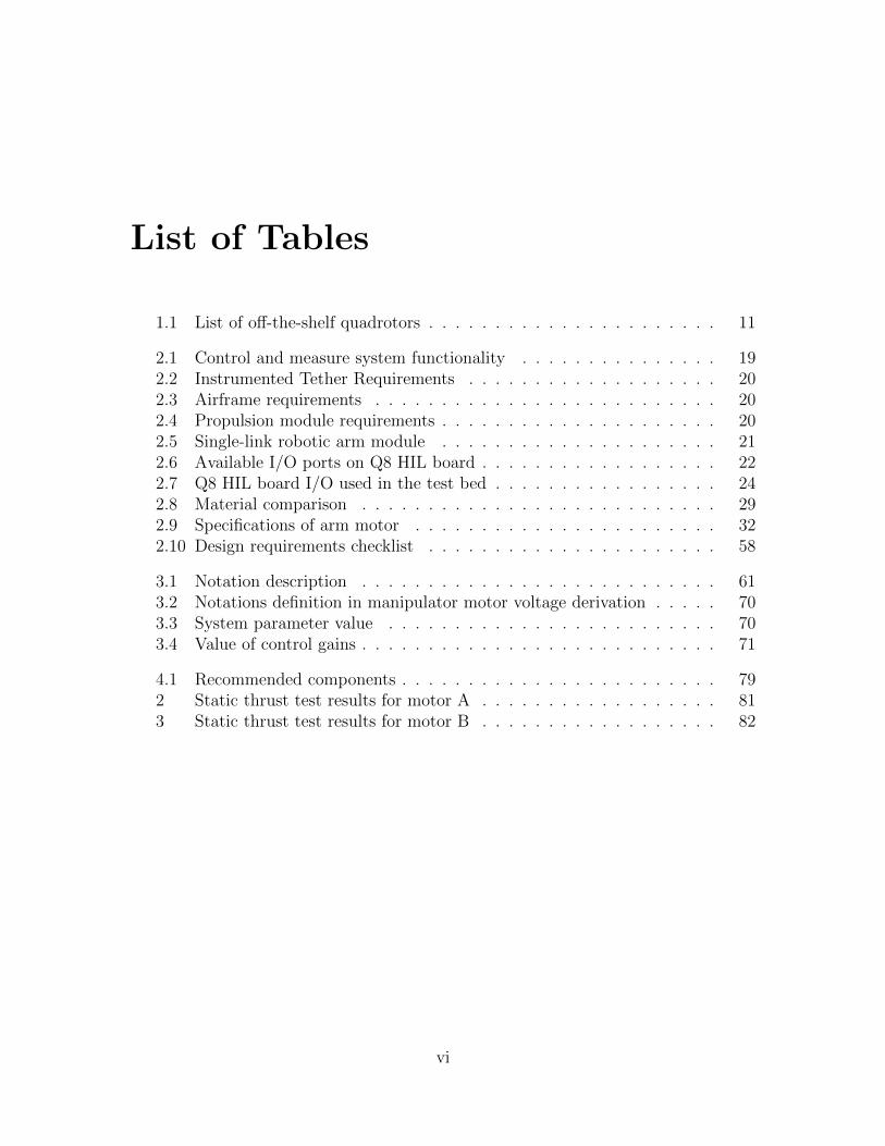
List of Tables
1.1 List of off-the-shelf quadrotors . . . . . . . . . . . . . . . . . . . . . . 11
2.1 Control and measure system functionality . . . . . . . . . . . . . . . 192.2 Instrumented Tether Requirements . . . . . . . . . . . . . . . . . . . 202.3 Airframe requirements . . . . . . . . . . . . . . . . . . . . . . . . . . 202.4 Propulsion module requirements . . . . . . . . . . . . . . . . . . . . . 202.5 Single-link robotic arm module . . . . . . . . . . . . . . . . . . . . . 212.6 Available I/O ports on Q8 HIL board . . . . . . . . . . . . . . . . . . 222.7 Q8 HIL board I/O used in the test bed . . . . . . . . . . . . . . . . . 242.8 Material comparison . . . . . . . . . . . . . . . . . . . . . . . . . . . 292.9 Specifications of arm motor . . . . . . . . . . . . . . . . . . . . . . . 322.10 Design requirements checklist . . . . . . . . . . . . . . . . . . . . . . 58
3.1 Notation description . . . . . . . . . . . . . . . . . . . . . . . . . . . 613.2 Notations definition in manipulator motor voltage derivation . . . . . 703.3 System parameter value . . . . . . . . . . . . . . . . . . . . . . . . . 703.4 Value of control gains . . . . . . . . . . . . . . . . . . . . . . . . . . . 71
4.1 Recommended components . . . . . . . . . . . . . . . . . . . . . . . . 792 Static thrust test results for motor A . . . . . . . . . . . . . . . . . . 813 Static thrust test results for motor B . . . . . . . . . . . . . . . . . . 82
vi

List of Figures
1.1 The Parrot AR Drone 2.0 is an example of the current class of smallUAVs available for civilian use. . . . . . . . . . . . . . . . . . . . . . 2
1.2 The primary advantage of mounting a manipulator arm on a UAV isthe nearly unlimited workspace. . . . . . . . . . . . . . . . . . . . . . 3
1.3 Potential applications of Unmanned Aerial Vehicles (UAVs) . . . . . 51.4 An illustration of difference between a redundant aerial manipulator
and a MOVA system. . . . . . . . . . . . . . . . . . . . . . . . . . . . 81.5 2D planar test bed allows planar motion (x- and z- directions) and roll
(θ) and rotation angle (α) of the manipulator. . . . . . . . . . . . . . 121.6 Testbed Schematic . . . . . . . . . . . . . . . . . . . . . . . . . . . . 13
2.1 System architecture . . . . . . . . . . . . . . . . . . . . . . . . . . . . 182.2 Q8 HIL board . . . . . . . . . . . . . . . . . . . . . . . . . . . . . . . 232.3 HIL control system using xPC Target . . . . . . . . . . . . . . . . . . 242.4 A schematic of spherical approximation of linear motion. Line AB is
the tangent line to the circular arc L at point A. . . . . . . . . . . . . 252.5 Two motor assembled as a universal joint . . . . . . . . . . . . . . . . 262.6 End of tether rotary joint connection . . . . . . . . . . . . . . . . . . 272.7 Airframe design . . . . . . . . . . . . . . . . . . . . . . . . . . . . . . 302.8 Airframe property evaluation . . . . . . . . . . . . . . . . . . . . . . 312.9 An illustration of Single-link robotic arm structure . . . . . . . . . . 322.10 Robotic arm and DC motor assembly . . . . . . . . . . . . . . . . . . 332.11 The Techron 5530 amplifier was set to operate at mono channel. . . . 342.12 An illustration of A2212 BLDC motor parts and dimension . . . . . . 352.13 Turnigy ESC wiring and PWM signal . . . . . . . . . . . . . . . . . . 362.14 Propeller balancer . . . . . . . . . . . . . . . . . . . . . . . . . . . . . 382.15 Static thrust test bench . . . . . . . . . . . . . . . . . . . . . . . . . 402.16 Static thrust test plot of two motors . . . . . . . . . . . . . . . . . . 412.17 Optical encoder . . . . . . . . . . . . . . . . . . . . . . . . . . . . . . 422.18 Speed sensor configuration . . . . . . . . . . . . . . . . . . . . . . . . 432.19 infrared diode circuit . . . . . . . . . . . . . . . . . . . . . . . . . . . 432.20 Plot of desired speed and actual speed at frequency 0.75 Hz . . . . . 442.21 Bode phase plot of ESC-motor system . . . . . . . . . . . . . . . . . 452.22 An illustration of the Phase Lead Compensator . . . . . . . . . . . . 46
vii

2.23 The encoder is mounted on a bracket, which is secured on the tetherlinkage by the clamp. . . . . . . . . . . . . . . . . . . . . . . . . . . . 48
2.24 A flow chart of using camera to measure MOVA attitude . . . . . . . 492.25 An illustration of camera setup . . . . . . . . . . . . . . . . . . . . . 502.26 A flow chart of the image processing algorithm . . . . . . . . . . . . . 522.27 Diagram of the PD Controller. . . . . . . . . . . . . . . . . . . . . . 542.28 Roll angle measurement of encoder and camera feedback from manual
test . . . . . . . . . . . . . . . . . . . . . . . . . . . . . . . . . . . . . 552.29 A comparison of derived velocity evaluation between encoder feedback
and camera feedback . . . . . . . . . . . . . . . . . . . . . . . . . . . 562.30 Comparison of controller position stabilization ability . . . . . . . . . 57
3.1 2D planar test bed . . . . . . . . . . . . . . . . . . . . . . . . . . . . 603.2 Experiment 1, VTOL aircraft hovered at initial position . . . . . . . . 723.3 Experiment 2, tracking pendulum motion trajectory . . . . . . . . . . 743.4 An illustration of the “wrenching a bolt” trajectory . . . . . . . . . . 753.5 Experiment 3, tracking inverted pendulum motion trajectory . . . . . 76
1 Side part of encoder bracket . . . . . . . . . . . . . . . . . . . . . . . 832 Front part of encoder bracket . . . . . . . . . . . . . . . . . . . . . . 833 Base part of encoder bracket . . . . . . . . . . . . . . . . . . . . . . . 844 Encoder bracket assembly drawing . . . . . . . . . . . . . . . . . . . 84
viii
Chapter 1
Introduction
1.1 Background
1.1.1 Unmanned Aerial Vehicle
Small Unmanned Aerial Vehicles (UAVs), for example the quadrotor shown
in Figure 1.1, are now extensively used in both civilian and military operations. The
rapid development of microcontrollers and sensing technology have made it feasi-
ble to deploy UAVs in both types of applications. Among all the types of UAVs,
small Vertical Takeoff and Landing (VTOL) aircraft have drawn increasing interest
because of their distinct maneuverability advantages over conventional fixed wing
aircraft in surveillance and inspection tasks. These tasks, such as searching, fire
detection, crop surveillance, and traffic inspection, may require a vehicle that can
loiter for detailed observation or fly close to fixed or moving obstacles. Modeling
and control algorithms for VTOLs have been investigated in many scientific works.
Proportional-integral-derivative (PID) controllers, with gain scheduling, are widely
used in controlling commercial UAVs [8]. More refined control algorithms that con-
1

sider the complete nonlinear system dynamics are under development. Sophisticated
techniques, such as integrator back-stepping approach, can be applied in the design
of such control systems [5].
Figure 1.1: The Parrot AR Drone 2.0 is an example of the current class of smallUAVs available for civilian use.
1.1.2 Mobile Manipulator
Manipulators or robotic arm mechanisms are similar to human arms that can
grasp and move objects. They can be programmed to operate autonomously or to
be manually controlled. A large number of manipulators have been designed in the
last sixty years and many of them have been widely used in industry. Manipulators
deployed on mass production lines are productive and helpful, but their fixed work
space has severely limited their suitable applications. In order to tackle new problems
and expand the flexibility of manipulator arms, manipulator arms have been combined
with mobile robot platforms.
Mounting a manipulator on a mobile platform to produce a mobile manipula-
tor is not a new idea, there have been research groups building mobile manipulators
for many years [16]. Currently most mobile manipulators are built on ground vehi-
2
cles and have been able to perform various practical tasks like bomb defusing and
space exploration. However, due to limitations of the mobile platforms, most of
these manipulator systems can only work on ground with smooth terrain. Also, large
supportive devices are demanded in large architectural structure inspections and con-
structions, such as factory chimney tests or tall building outside wall maintenance,
when ground-based mobile manipulators are used.
1.1.3 UAV Borne Manipulator
In most current UAV applications, the UAV is used only as a carrier for en-
vironment sensors or a video acquisition device. The idea of mounting a robotic
manipulator on a UAV such that it is able to interact with other objects reveals great
potential for UAVs in even more applications.
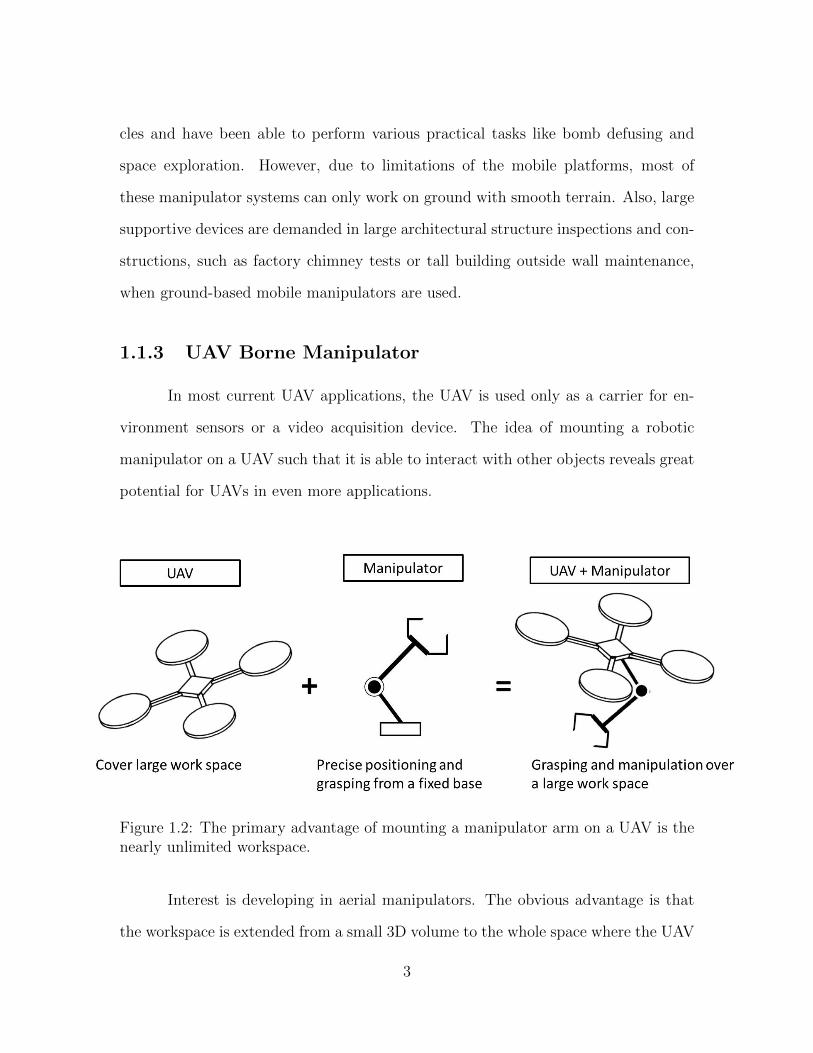
Figure 1.2: The primary advantage of mounting a manipulator arm on a UAV is thenearly unlimited workspace.
Interest is developing in aerial manipulators. The obvious advantage is that
the workspace is extended from a small 3D volume to the whole space where the UAV
3

can travel (Figure 1.2). Such a system has the dexterity of the manipulator plus better
mobility compared to the ground-based mobile manipulator. As a host platform, the
VTOL can be deployed at places that are inaccessible for ground mobile manipulators,
allowing the manipulator attached on the VTOL aircraft to interact with the remote
environment. Potential tasks include tall buildings or bridge maintenance, material
sample collection from complex terrain, and package delivery (Figure 1.3). Even
for those tasks that are currently undertaken by ground manipulators, the agility
of VTOL aircraft in narrow spaces and the fast travel speed regardless of terrain
complexity could provide better performance.
4

(a) Factory chimney inspection(b) Tall building outside wall mainte-nance
(c) Fighting a fire (d) Defusing a bomb
Figure 1.3: Potential applications of Unmanned Aerial Vehicles (UAVs)
While equipping VTOL with robotic arm has great potential in various ap-
plications, very few control algorithms are developed to harness the performance of
such an integrated system efficiently. Challenges still exist before VTOL aircraft and
robotic arms can truly be integrated together and fulfill the potential of such sys-
tems. One important issue has to do with the underactuated nature of the VTOL
5

aircraft. Underactuated refers to a system in which not all of its degree-of-freedom
(DOF) could be independently controlled, there are fewer independent control ac-
tuators than the total DOF. Specifically for the quadrotor aircraft, among the six
degree-of-freedom of the VTOL, only four of them can be controlled separately while
the x- and y- position are not directly controllable. The unique problem of control-
ling an aerial vehicle with an attached manipulator is that the internal force and
torque generated by the interaction between the arm and the host VTOL may not
be negligible depending on the relative mass of the two subsystems. Such interaction
adds to the complexity of the dynamics model of the whole system and is difficult
to stabilize when designing a controller. Secondly, operating from a hovering VTOL
aircraft makes the end-effector difficult to perform fine motions to target the object
of interest precisely.
Another issue in constructing a UAV borne manipulator is the flight time.
Since for most application scenarios, like searching and rescuing, VTOLs equipped
with robotic arms are required to operate through a long distance, the flight time is
one of the most critical factors. While a heavy host VTOL, renders the system less
susceptible to interaction with the onboard manipulator, it will consume more energy
thus resulting in shorter flight time. The manipulator design must balance func-
tionality (often redundancy) of the manipulator against weight of the manipulator.
Redundant links, although helpful to position the robot at arbitrary configurations
for manipulation tasks, add to the total weight and draw extra energy while operating
and transporting.
There are some researchers trying to address the above issues. The GRASP
research team of University of Pennsylvania has used a fleet of quadrotors to perform
cooperative assembly work [6]. Pounds et al. used PID controllers to stablize the
host UAV, taking the change of load mass as disturbance [8]. They determine a
6

bound within which changing load mass will not destabilize the aircraft. However
only a grasper is attached under the aircraft for object retrieval and the accuracy of
tracking trajectory while carrying an object is not discussed in this paper. Another
group has mounted and controlled a multi-link manipulator on a VTOL UAV [1].
Redundant degrees-of-freedom (DOF) for the manipulator or host UAV are required
to compensate for the interactive torque within the system, i.e. extra weight and
complexity is added to the system in order to compensate for what is likely a control
design issue. Yet the total weight along with the cost will increase for the redundant
actuators, which are not discussed in the paper either.
1.1.4 New Design of Manipulator on VTOL Aircraft(MOVA)
In regard to the above issues, one efficient way to extend the flight time is
to minimize the weight of the manipulator, that is, use only the necessary number
of actuators for the system. Specifically for a quadrotor, utilize the four degree-of-
freedom VTOL aircraft coupled with a two degree-of-freedom manipulator to generate
a six degree-of-freedom aerial manipulator system.
A challenge of realizing the potential benefits of the VTOL + manipulator
system involves managing the interaction of the onboard manipulator and the VTOL
aircraft–the dynamics of both subsystems may be profoundly affected by each other,
depending on relative masses and moment of inertia. When deriving a dynamic
model of the complete system by directly applying Euler-Lagrangian approach, cou-
pled terms that neither belong to the aircraft nor the manipulator are produced.
These complex coupling terms represent the interaction between two subsystems and
add to the difficulty in control algorithm design [14].
The typical control design approach has been to acknowledge that this phe-
7

nomenon exists but design controllers that only implicitly address these forces, e.g.
design an aircraft body controller that is robust to these disturbances. To explicitly
approach the challenge, Xu et al. designed an innovative aerial mobile manipulator,
referred to as MOVA [12], which stands for Manipulator on VTOL (Vertical Take-Off
and Landing) Aircraft. In preparation for developing MOVA control algorithm in 3-
dimensional (3D) space, the dynamic equation and control algorithm of 2D model was
investigated in Xu’s work. The planar MOVA system has minimal number of joints
for the end-effector to achieve trajectory tracking. Figure 1.4 illustrates the difference
between a redundant manipulator and the MOVA approach. Through virtual manip-
ulator method, dynamics of the MOVA system are transformed into a form that has
decoupled translational and rotational dynamics. The resulted dynamic equations
facilitate the controller design. After deriving the decoupled dynamic equation, the
paper describes a unified back-stepping controller for the integrated system.
Figure 1.4: An illustration of difference between a redundant aerial manipulator anda MOVA system.
8

1.2 Problem Statement
Controlling the VTOL aircraft and the manipulator through one unified con-
troller is a new idea, it is very appealing to run physical tests for the system and
demonstrate the interesting points in the MOVA control algorithm such as the active
compensation for interactions between the VTOL and the manipulator. An experi-
mental test-bed for validation of the MOVA system is needed.
1.2.1 Test bed Motion Constraint
Many UAV tests are performed using outdoor test facilities where reliable
on-board navigation systems are required, such as GPS, gyros, accelerometers and
magnetometers. There are great advantages to outdoor experiments yet they can
be considerably expensive due to the number of the sensors and data acquisition
devices. Outdoor UAV experiments must be performed in a wide open area by well
trained personnel and are vulnerable to weather conditions. Compared to indoor tests,
all those factors render the outdoor tests less appealing to researchers subjected to
limited funding or work site constraints. By using small or mini UAVs and using
external (off-board) position and attitude estimate, indoor tests could be performed
at anytime, and experimental results can be analyzed instantly.
Considering potential crash scenarios during the tests, the safety of personnel
and devices around the test become the most important factor when deciding on the
type of facility to use. A fail-safe configuration and simple mechanical design are
desirable for a test bed.
A tether configuration that constrains motion of a UAV under test within a
2-dimensional (2D) plane is proposed. Due to the difficulty of physically realizing
a 2D plane motion, a spherical approximation is made by connecting the UAV to a
9

fixed point through a long radius. Q8 Hardware-In-the-Loop (HIL) Board and xPC
Target are used to process the feedback signal from sensors incorporated in the tether
and command the outputs. Simulink R© is used to implement the control algorithm.
1.2.2 UAV Platform for Testing
Among all the VTOL vehicles, quad-copters, or also called quadrotors are more
suitable than tail rotor helicopters as indoor test platforms. A quadrotor is lifted by
two sets of identical and symmetrically arranged propellers. Other than simplicity
of control, it has simpler machine construction than a comparably scaled helicopter
as well as smaller sized propellers, which could reduce the damage caused should the
vehicle is out of control.
At the moment there are no commercial UAV quadrotors mounted with robotic
arms on the market. Such test beds when needed are usually modified and developed
from a few quadrotor platforms. One of the most notable platform models is the
AR.Drone produced by Parrot. There are also Hummingbird, Dragonflyer and a
few other commercial quadcoptors that are suitable for research. Some of the most
popular commercial quadrotors used by research institutes are listed in Table 1.1.
The AR. Drone is favored by many research groups. It has two cameras
therefore and could be used to perform vision experiments. But its frame size is
rather too large for indoor experiments. Its limited lifting force and compact body
size limit the ability for further modifications. While the Hummingbird, IRIS and
Dragonflyer are compact in size they are more expensive.
Although the above listed products demonstrate good versatility with Global
Positioning System (GPS) and provide on-board micro-controllers for different levels
user customization, they are mostly for outdoor experiments and many of the sensors
10

Model Size Features Price (USD)A.R. Drone 2.0 820mm × 820mm 1. Equipped with camera of
1280 × 7202. Triple axis gyroscope3. Triple axis accerlerome-ter4. Triple axis magnetome-ter5. Pressure sensor6. Ultrasound sensor
$ 200 or above
Hummingbird 540mm × 540mm 1.Autopilot developing tool2. Extendable3. Compact size suitable forindoor test4. Triple axis magnetome-ter
$ 500 or above
IRIS 600mm × 600mm 1. Programmable autopilot2. Magnetometer
$ 750 or above
DragonflyerShadow
502mm × 502mm 1. Flight data recorder2. Accelerometer3. Gyroscope4. Pressure sensor
$ 2995 or above
Table 1.1: List of off-the-shelf quadrotors
on-board (GPS and magnetometer) appear to be useless for indoor tests. More im-
portantly the unmodifiable mechanical configurations allow neither extra mounting
points nor larger lifting force for on-board robotic manipulator.
A planar 2D test bed of a small UAV + manipulator is proposed. The test bed
consists of a three degree-of-freedom, two dimensional host VTOL and a single link
manipulator. Two propellers are used because redundant actuators yield undesirable
torque about the yaw axis, which can lead to instability. The UAV and manipula-
11

tor, along with the proposed tether, constitute a complete test bed for the UAV +
manipulator controller evaluation (Figure 1.5).
Figure 1.5: 2D planar test bed allows planar motion (x- and z- directions) and roll(θ) and rotation angle (α) of the manipulator.
1.3 Related Works
While there are no established test beds that can be directly used for the
MOVA system, the development of an open source UAV platform would allow re-
searchers to adapt and modify UAVs cater to specific aims. The GRASP research
team of University of Pennsylvania has developed a test bed to test multirobot aerial
control algorithms using the Hummingbird quadrotor [6]. Another group modified Q4
Dragster frame from Lipoly.de to support a direct approximate-adaptive control [7].
The quadrotor was constrained in Z- direction by being mounted on a spherical bear-
ing allowing only yaw and limited rolled and pitch motion. In Tayebi and McGilvray’s
paper [9], experimental tests were performed on a modified Draganflyer III from RC
Toy. A stationary ball joint base is attached to the quadrotor and a dSPACE DS1104
R&D board is used to control it. In their experiments, motor speed is measured by
12

Hall-effect sensors. Hoffman, Goddenmeier and Bertram used a test bed mounted
on a gimbal to compare proportional-integral-derivative (PID) and Integrator back-
stepping controllers [2]. Instead of being modified from commercial quadrotor, the
test bed is not a real quadrotor but constructed using light weight frame along with
electronic components. Yu and Ding designed a test bench mounted on a fixed base
through a sphere joint [11]. The test bench also includes 6 axes torque/force sensor
to measure dynamics of motor-propeller subsystems.
All of the above test beds constrain the main body (Figure 1.6) at a fixed
point. Such constraints keep the test bed safe to operate. But in order to fully
evaluate the control algorithm, the test bed should also allow the aircraft to track
trajectories in the space and demonstrate the action of a controller under a real flying
conditions. Ability to record flying data such as pitch angle and translational speed
is also required.
Figure 1.6: Testbed Schematic
In addition to indoor VTOL test beds, other research groups have mounted
multi-link arm on outdoor UAVs. The Vision and Control Group from University of
Seville presents a quadrotor with an arm for assembly tasks [3]. The new platform is
used to test an Integrator back-stepping controller that takes into account the motion
13

of the arm. Korpela et al. describes a design of miniature gantry crane mounted on
a large UAV [4].
In sum, indoor test beds have the distinctive advantage of low cost and im-
munity to weather influence. Many research groups use test beds modified from
quadrotor or multi-rotor because of their simple mechanical construction control con-
venience. But most of the self-modified test beds can only measure flying attitude
instead of demonstrating a real flying condition. Although commercial quadrotors for
hobbyists provide good versatility and refined frame, they have little room for modi-
fication to meet user specified requirements. Building a new test bed is low cost and
could be modified according to future needs. Certain constraints should be applied
to the VTOL vehicle to keep the test bed operating in a safe area. The constraints
should also allow the aircraft to fly sufficient freedom for complete testing.
1.4 Organization
The first chapter provides a background introduction of UAV and aerial ma-
nipulator. In particular the integrated UAV and manipulator system, referred to as
MOVA, is presented. The need for a MOVA test bed is stated and some related test
beds are introduced. The overall design of the proposed work is thus motivated.
In Chapter 2, system architecture is illustrated following a top down functional
decomposition method. All functional modules are described, including two attitude
position measurement methods: 1). using encoders in the mechanical tether that
are attached to the host VTOL helicopter and manipulator actuator to measure and
derive position of the end-effector; and 2). via image processing using a camera
as a sensor for position measurement. Comparison between the two methods are
performed and results are discussed. In Chapter 3, a controller that applies the same
14
back-stepping technique as MOVA but based on a conventional Euler-Lagrangian
approach derived dynamic model is described and implemented. The performance
of the controller is compared with the MOVA controller. Results of maintaining at
fixed positions and tracking different end-effector trajectories are presented. The last
chapter summarizes the achievements of the proposed work. Possible improvements
on the test bed and suggestions for future work are presented.
15

Chapter 2
2D Planar Test bed Design
The design of the test bed instrumentation and hardware are described via
functional decomposition in this chapter. The first section introduces the system ar-
chitecture. Five subsystems that constitute the test bed system are introduced and
the requirements are defined. The second section presents the control software and
hardware: the Q8 hardware-in-the-loop (HIL) board, the Host PC and the software
environment Mathworks xPC Target. The air frame design and the material selection
are explained in the third section. The tether used to constrain the UAV movement,
position sensor and single-link robotic arm module are detailed. The following section
focuses on the propulsion module, the brushless DC drive motor and electronic speed
controller (ESC) and its control interface are described in this section. Tests that
measure propeller static thrust and measurement of the frequency response are elab-
orated in Section 5. In the last section, two methods of attitude estimation, rotary
encoder at the end of the tether and a camera-based system, are described and their
performances are compared and discussed.
16

2.1 System Architecture
The objective is to design and build a two-dimensional test bed for UAV
controller testing and a prototype 3 DOF Manipulator On a VTOL Aircraft (MOVA).
In order to execute the design process, the system is divided into modules that serve
specific functions. The two main systems are the instrumented tether, including
UAV control hardware and software, and the UAV under test. Five subsystems and
their interactions that define the system architecture are presented in Figure 2.1. The
control algorithm runs on the xPC Target PC and interacts with the hardware through
the Quanser Q8 board. The Q8 board reads in VTOL position and VTOL attitude
from position sensors, and issues commands to the robotic arm and propulsion units
to bring the end-effector to a desired position. Requirements of each subsystem are
detailed in the following subsections.
17

Figure 2.1: System architecture
2.1.1 Control and Position Estimation
To implement UAV controller on the test bed, a data acquisition and control
platform is required to take in multiple sensor inputs, estimate the system states,
evaluate the control algorithm and output analog or digital commands to the UAV
under test. The control system should be able to generate command signals at least
100 times per second to guarantee sufficient flight control. An algorithm, implemented
in the control system software, will perform system position evaluation. The inputs
and outputs of the control module are listed in Table 2.1.
18

Module Control and Measurement ModuleInputs Quadrature TTL signal from encoder with 4 channels
VTOL roll angle data from encoder (+90 to -90 degree)Manipulator direction from userTether linkage position α and βUAV attitude θ0Data from camera
Outputs Pulse width modulation (PWM) signal for servo control(standard hobby servo interface)Analog control signal: -5V to +5V with at least 10-bitresolution
Functionality Input sensor feedback, derive system position, computeand execute control algorithm
Table 2.1: Control and measure system functionality
2.1.2 Instrumented Tether
A tether will be designed to estimate the motion of the airframe and constrain
the range of motion of the UAV under test. The system transnational position and
sensing devices should be incorporated into the tether. Encoder sensor will be in-
cluded in the tether but may add significant weight. An alternate sensor such as a
camera may be feasible but may introduce extra noise to the system and be con-
strained by update rate. This alternate sensing approach will be investigated during
the design process and a comparison test will be performed. For a sufficient position
feedback, the position sensor and attitude sensor should have a resolution of at least
5 mm and 0.02 radian respectively.
2.1.3 Airframe
The air frame serves as a platform upon which the propulsion module and
arm module are built. The frame should be compact and light weight. Appropriate
rigidness is also required for the MOVA to survive vibration or even minor impact.
19
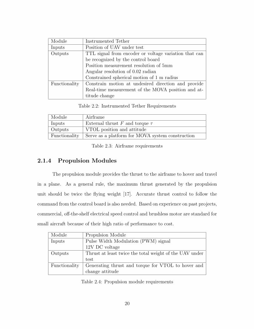
Module Instrumented TetherInputs Position of UAV under testOutputs TTL signal from encoder or voltage variation that can
be recognized by the control boardPosition measurement resolution of 5mmAngular resolution of 0.02 radianConstrained spherical motion of 1 m radius
Functionality Constrain motion at undesired direction and provideReal-time measurement of the MOVA position and at-titude change
Table 2.2: Instrumented Tether Requirements
Module AirframeInputs External thrust F and torque τOutputs VTOL position and attitudeFunctionality Serve as a platform for MOVA system construction
Table 2.3: Airframe requirements
2.1.4 Propulsion Modules
The propulsion module provides the thrust to the airframe to hover and travel
in a plane. As a general rule, the maximum thrust generated by the propulsion
unit should be twice the flying weight [17]. Accurate thrust control to follow the
command from the control board is also needed. Based on experience on past projects,
commercial, off-the-shelf electrical speed control and brushless motor are standard for
small aircraft because of their high ratio of performance to cost.
Module Propulsion ModuleInputs Pulse Width Modulation (PWM) signal
12V DC voltageOutputs Thrust at least twice the total weight of the UAV under
testFunctionality Generating thrust and torque for VTOL to hover and
change attitude
Table 2.4: Propulsion module requirements
20

2.1.5 Single-link Robotic Arm Module
The single-link robotic arm should possess appropriate mass and rotational
inertia such that the interaction between the VTOL and arm can be observed while
the VTOL is hovering. A DC motor is the most likely candidate as the arm actuator
because of its compact size, high reliability and simple control. For configuration
simplicity, a motor with built in encoder to measure the arm position is preferable.
A programmable voltage amplifier is needed to transform AC supply voltage and the
control signal into an appropriate DC voltage for the motor.
Module Single-link robotic arm moduleInputs 120V AC voltage to the amplifier
Analog control signal from the control board: -5V to+5V
Outputs End-effector position as quadrotor encoder outputFunctionality Represent the robotic arm in the MOVA system
Table 2.5: Single-link robotic arm module
2.2 Control System
Q8 Hardware-in-the-Loop (HIL) Board and xPC TargetTM are used as the real-
time control system of the test bed. This hardware/software system is standard in the
controls and robotics laboratory and was selected without additional consideration.
2.2.1 xPC TargetTM and xPC Target Workstation
xPC TargetTM is a real-time software environment from MathWorks Inc. which
runs on a computer workstation without an operating system (eg. Microsoft Win-
dows). It allows the user to run Simulink R© generated models in a separate PC based
21

workstation and provides a library of I/O drivers and a real-time kernel. The fea-
tures of real-time monitoring, parameter tuning, and data logging make it an ideal
environment for a control system test bed.
xPC Target software requires a Host computer, a Target computer and com-
patible I/O boards. The I/O board will be introduced in next subsection. Simulink
models and executable code are constructed on the Host computer and then down-
loaded to the target computer for execution. In the proposed work, a Lenovo Y580
laptop computer is used as the Host computer.
2.2.2 Q8 HIL Board
The Quanser Q8 Hardware-In-the-Loop (HIL) board serves as an I/O board
in the control system. It reads in system states and outputs control signals. The
Q8 board is a peripheral component interconnection (PCI) based device that offers
wide variety of I/O abilities (Table 2.6). Q8 HIL board has two parts-the main card
and the terminal board. The main card (Figure 2.2a) is inserted into a PCI slot on
the mother board of the Target workstation. The main card connects, through two
44-pin ribbon cables and one 50-pin ribbon cable, to the Q8 terminal board (Figure
2.2b), which has all the interfacing connectors. The input/output ports on Q8 HIL
terminal card used in the proposed work are listed in Table 2.7.
8 x 14 bit Analog Inputs8 x 12 bit D/A Outputs
8 Quadrature Encoder Inputs32 Programmable Digital IO Channels2 x 32 bit dedicated Counter/ Timers
2 External Interrupt sources32 bit, 33MHz PCI Bus Interface
Table 2.6: Available I/O ports on Q8 HIL board
22

(a) main board
(b) terminal board
Figure 2.2: Q8 HIL board
2.2.3 Control Software
MATLAB Simulink is used to create a model of the control system. The model
is then compiled as executable code and downloaded from the Host PC to the xPC
Target workstation through an Ethernet connection. The model is run by xPC Target
in real time, which communicates through the Q8 HIL board with test bed hardware,
receiving sensor inputs and issuing commands. While the model is running, data can
be stored in the memory of the Target workstation for offline analysis or shipped back
to the host laptop for real-time display. A schematic of the control system is shown
in Figure 2.3. Some sensors, such as the camera, can operate from the Host computer
23

I/O ports Functionality4x Encoder input Recieve MOVA position (2 ports)
Receive MOVA attitudeReceive robotic arm position
1x Analog output Issue voltage signal to onboard arm actuatorCounter/Watchdogoutput
Issue pulse width modulation signal to control brushlessmotor
Table 2.7: Q8 HIL board I/O used in the test bed
and the data is then transmitted to the control program on the Target computer
Figure 2.3: HIL control system using xPC Target
2.3 Instrumented Tether
Considering it is difficult to achieve a strictly planar movement, a spherical
approximation is proposed. The aerial vehicle’s motion is constrained by a tether
which consists of a lightweight rod with a gimbal fixed to the ground at one end, and
the other end is a rotary joint that provides the mounting point for the UAV under
test. Such a connection constrains the yaw and pitch movement, leaving only the roll
rotation to be performed by the MOVA. The tether is designed to be 1000 mm long,
24

and the airframe movement range is a 800×800 mm rectangle. The approximation
along the x-axis is shown in Figure 2.4.
Figure 2.4: A schematic of spherical approximation of linear motion. Line AB is thetangent line to the circular arc L at point A.
The angle θ dictates the approximation of the linear motion. That is the
smaller θ is, the more the actual arc approximates the imaginary line. Based on the
law of cosines, l2 = l2 +D2 − 2lDcosα cosα can be found by
cosα =D
2l= 0.4. (2.1)
As tangent line AB is perpendicular to the radius OA, cosα = sinθ.
θ = sin−10.4 = 0.411radian. (2.2)
25
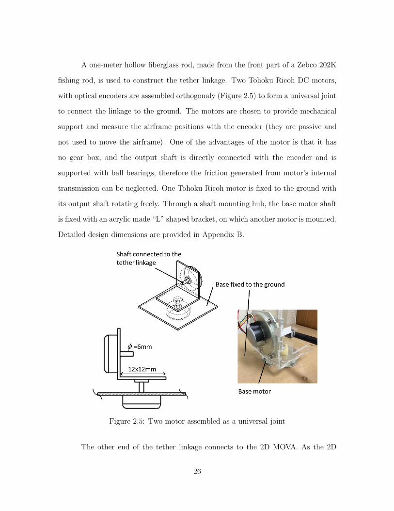
A one-meter hollow fiberglass rod, made from the front part of a Zebco 202K
fishing rod, is used to construct the tether linkage. Two Tohoku Ricoh DC motors,
with optical encoders are assembled orthogonaly (Figure 2.5) to form a universal joint
to connect the linkage to the ground. The motors are chosen to provide mechanical
support and measure the airframe positions with the encoder (they are passive and
not used to move the airframe). One of the advantages of the motor is that it has
no gear box, and the output shaft is directly connected with the encoder and is
supported with ball bearings, therefore the friction generated from motor’s internal
transmission can be neglected. One Tohoku Ricoh motor is fixed to the ground with
its output shaft rotating freely. Through a shaft mounting hub, the base motor shaft
is fixed with an acrylic made “L” shaped bracket, on which another motor is mounted.
Detailed design dimensions are provided in Appendix B.
Figure 2.5: Two motor assembled as a universal joint
The other end of the tether linkage connects to the 2D MOVA. As the 2D
26

MOVA moves up and down (along z- axis), the upper motor shaft is turned. Likewise
the base motor shaft turns as the linkage moves sideways (along the x- axis). Through
this mechanism, the position of UAV under test in a plane can be computed from
the measurement of the motor encoders. Given that they are quadrature encoder
resolution of 400 counts square wave per revolution, the position measuring resolution
is computed as:
r =2π
4× 400= 3.925mm/count. (2.3)
Therefore the position sensor meets the requirement in section 2.1.2.
The tether linkage end that connects to a UAV under test has an outer diam-
eter of 8 mm. Two ball bearings with inner diameter of 8 mm are utilized to form
the rotating joint between the 2D MOVA body and the rod to allow unconstrained
roll motion. A bracket made of acrylic integrated into the airframe design, is used
to secure the bearings. The mechanism (shown in Figure 2.6) prevents movement
around the yaw and pitch axes.
Figure 2.6: End of tether rotary joint connection
27

2.4 Planar MOVA Airframe and Single-link Robotic
Arm Design
The planar MOVA host airframe is constructed as “half” of a quadrotor. It is
slightly different from simply dividing a quadrotor, in that it has two symmetrically
arranged propellers. They are used in flight control to provide the twisting torque
and lift force. The 2D MOVA can only fly along the x-axis and y-axis, in a plane, by
adjusting rolling angle and thrust. An on-board actuator will be added to construct
a single-link robot. A robotic arm with mass comparable to the host UAV is attached
on the actuator. The 2D planar MOVA has 3 DOF from UAV + 1 DOF from
manipulator = 4 DOF.
2.4.1 Airframe Design
Weight plays an important role in the UAV design. With two propellers the
UAV’s weight-to-thrust ratio would be less than half of that of the quad-copter.
Enough thrust margin for good maneuverability could be guaranteed by using lightweight
material and appropriate mechanical design. Another mandatory requirement is
machinability-the airframe should be easily modified or shaped to meet any special
needs.
Different materials have merits that help to meet the above requirements.
Three materials are considered in the design—acrylic, aluminum and carbon fiber.
Their properties are listed in Table 2.8. Aluminum and carbon fiber are favored by
aviation hobbyists for their durability. Yet the aluminum is too heavy for a mini
indoor test bed while the carbon fiber tubes are difficult to machine. On the other
hand, the acrylic is light weight, has appropriate strength and can be easily cut into
28

desire shape by a laser cutter. Therefore the acrylic is suitable for the frame and was
chosen as the only material used in the frame. All acrylic parts in this work were
machined using the Versalaser Portable Desktop Laser Engraver, manufactured by
Universal Laser System.
Material Density StrengthAluminum [22] 2.7 g cm−2 High
Carbon fiber [23] 1.55 g cm−2 HighAcrylic [25] 1.18 g cm−2 Medium
Table 2.8: Material comparison
Given the limited thrust of only two propellers, the frame of the UAV is
designed in a most efficient way. That is, the frame is designed to be as narrow
as possible to support only necessary devices such as the end-effector actuator. To
minimize weight the power supply and the control board will be off-board the UAV.
The frame is designed as a symmetric “dumbbell”” shape with a rectangle at the
middle (Figure 2.7). The motors are mounted on the end of each arm. Two identical
frame layers are cut and assembled together through two ribs to enhance the rigidness
of the structure. The length of the frame, which is also the distance of two propellers
was set to 300 mm.
29

Figure 2.7: Airframe design
A three dimensional model of the MOVA without the robotic arm was con-
structed and its properties were evaluated using Solidworks R© 3D CAD design software
(Figure 2.8). The overall mass is 178.91 grams and the moment of inertia taken at the
roll axis is 1306.0337 kg mm2. The properties will be referenced in the arm design.
30

Figure 2.8: Airframe property evaluation
2.4.2 Single-link Robotic Arm Design
The robotic arm is designed as a “pendulum” shape. One of its ends will
be attached to the motor on the frame so that the arm can turn like a pendulum to
provide the interaction with the VTOL aerial vehicle. To test the MOVA performance
under different levels of interaction, the mass and moment of inertia can be changed.
The arm consists of three layers. Slots for screws are cut at the middle of each layer
such that the middle layer can slide back and forth to adjust the length of the arm
(Figure 2.9). The moment of inertia varies as the length changes. The layers can be
secured in place by tightening the nuts.
A DC motor [21], is selected to drive the arm. It has an integrated quadrature
optical encoder which provides a resolution of 64 counts per revolution. Considering
31

Figure 2.9: An illustration of Single-link robotic arm structure
its gear ratio, the resolution at the motor output shaft is 1216 counts per revolution,
which is 2.72× 10⁻⁴ radian per count. The resolution greatly exceeds that of the
position sensor, thus it fulfills the measuring requirements. Including the DC motor,
the single-link robotic arm weighs 128 grams. The overall 2D MOVA weighs as 310
gram. Figure 2.10 shows the assembled robotic arm module. The motor specifications
can be found in Table 2.9. Note that the rated voltage is 12 V but the motor will be
operated in the range 6 V to 12 V. The arm motor specifications will be referenced
in Chapter 3.
Ratedvoltage
Gear ra-tio
No-loadspeed
Stall torque atrated voltage
Stall cur-rent atratedvoltage
Size
12V 19:1 500RPM 0.593N.m 5A 37D x 52Lmm
6V 19:1 256RPM 0.297N.m 0.25A 37D x 52Lmm
Table 2.9: Specifications of arm motor
32

Figure 2.10: Robotic arm and DC motor assembly
2.4.3 Linear Power Amplifier
In order to output a variable voltage to move the DC motor, a programmable
power amplifier is needed to connect the Q8 analog output and the actuator of the
end-effector. The amplifier model used in the test bed is Techron 5530. It is able to
deliver power from DC to 20 KHz under single channel mode. The maximum DC
output is 10A at 100V. Calibration is required to perform a unity voltage gain. The
wiring of the amplifier can be found in Figure 2.11.
2.5 Propulsion Module Design
2.5.1 Brushless DC Motor
Brushless DC (BLDC) motors are popular motors for model aircraft including
quadcopter, due to their large power-to-weight ratio and low cost. Two BLDC motors
used in the test bed are the A2212 Brushless Outrunner Motor (Figure 2.12). The
33
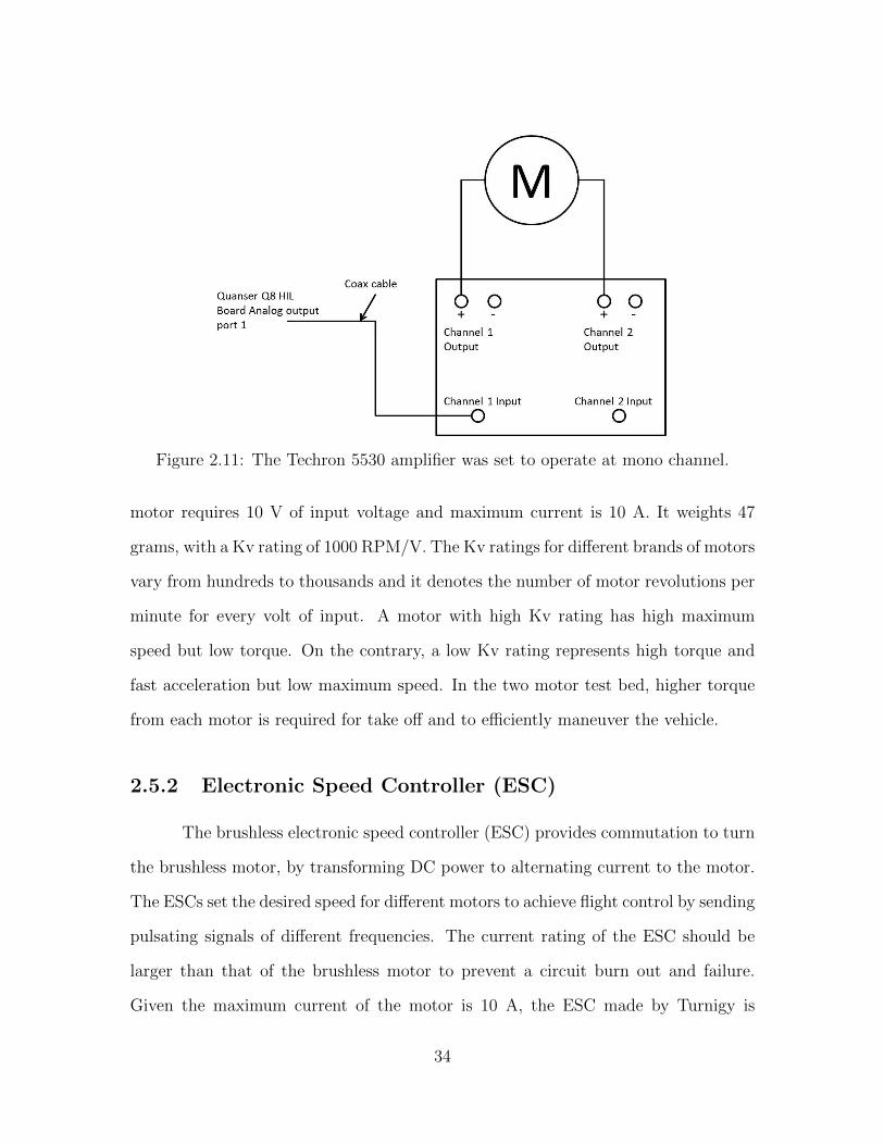
Figure 2.11: The Techron 5530 amplifier was set to operate at mono channel.
motor requires 10 V of input voltage and maximum current is 10 A. It weights 47
grams, with a Kv rating of 1000 RPM/V. The Kv ratings for different brands of motors
vary from hundreds to thousands and it denotes the number of motor revolutions per
minute for every volt of input. A motor with high Kv rating has high maximum
speed but low torque. On the contrary, a low Kv rating represents high torque and
fast acceleration but low maximum speed. In the two motor test bed, higher torque
from each motor is required for take off and to efficiently maneuver the vehicle.
2.5.2 Electronic Speed Controller (ESC)
The brushless electronic speed controller (ESC) provides commutation to turn
the brushless motor, by transforming DC power to alternating current to the motor.
The ESCs set the desired speed for different motors to achieve flight control by sending
pulsating signals of different frequencies. The current rating of the ESC should be
larger than that of the brushless motor to prevent a circuit burn out and failure.
Given the maximum current of the motor is 10 A, the ESC made by Turnigy is
34
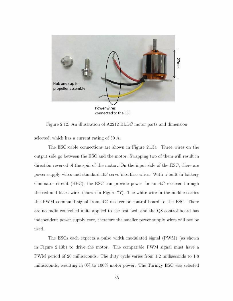
Figure 2.12: An illustration of A2212 BLDC motor parts and dimension
selected, which has a current rating of 30 A.
The ESC cable connections are shown in Figure 2.13a. Three wires on the
output side go between the ESC and the motor. Swapping two of them will result in
direction reversal of the spin of the motor. On the input side of the ESC, there are
power supply wires and standard RC servo interface wires. With a built in battery
eliminator circuit (BEC), the ESC can provide power for an RC receiver through
the red and black wires (shown in Figure ??). The white wire in the middle carries
the PWM command signal from RC receiver or control board to the ESC. There
are no radio controlled units applied to the test bed, and the Q8 control board has
independent power supply core, therefore the smaller power supply wires will not be
used.
The ESCs each expects a pulse width modulated signal (PWM) (as shown
in Figure 2.13b) to drive the motor. The compatible PWM signal must have a
PWM period of 20 milliseconds. The duty cycle varies from 1.2 milliseconds to 1.8
milliseconds, resulting in 0% to 100% motor power. The Turnigy ESC was selected
35

to control the BLDC motor on the 2D MOVA. The Turnigy ESC supports higher
PWM frequency up to 500 Hz; compared to the 1000 Hz xPC sampling rate, it is a
good match.
(a) An illustration of ESC wiring
(b) PWM signal
Figure 2.13: Turnigy ESC wiring and PWM signal
2.5.3 Power Supply
The power source for the ESC is a 110V AC to DC power supply with output
DC voltage 12V with maximum power of 36 Watts. It provides three DC outputs.
The power supply replaces batteries that are normally used in model aircraft and
provides stable voltage to the motor.
36

2.5.4 Propeller Selection
The 2D MOVA uses one clockwise and one counter-clockwise propeller. They
spin in different direction to counter balance the torque generated on the yaw axis.
Propellers have two key specifications–length and pitch. The length is measured
tip to tip while pitch denotes the advancing distance in one revolution. Generally
speaking, long length creates high thrust but is slow in response due to the larger
inertia, while large pitch provides large acceleration yet may create turbulence. Other
factors, such as material, weight, blade number, motor power, with length and pitch
together determine the stability and agility of a VTOL.
It is difficult to find an ideal combination of BLDC motor and propeller through
computation. As a general rule, a motor with Kv rating of 900-1000 can drive a
propeller 10 inches long and 4.5 to 6 inches pitch. For an indoor test bed, stability
is the first priority. Small pitch helps to reduce vibration and turbulence that cause
the VTOL to wobble when hovering. So the pitch of the propeller is chosen to be 4.5
inches. Considering a large propeller with light weight can produce fast step response,
and a soft material improves the MOVA safety, a pair of Maxx Product 10 (length in
inch) x 4.5 (pitch in inch) EPP1045, plastic propellers was selected to mount on the
motor.
None of the propellers on the market are perfectly balanced. Unbalanced pro-
pellers yield considerably large vibration. Such vibration travels through the entire
air frame and introduces harmful noise to the onboard sensors and may even damage
the motor bearings and parts. Propeller balancing reduces the vibration thus signif-
icantly improves the overall system stability and elongates the parts longevity. This
was done using a balancer (Figure 2.14). The propeller is installed on the balancer
shaft and the blade is aligned horizontally. If it rotates out of the horizontal align-
37

ment, material removal from the heavy side of the blade is needed. Sandpaper was
used to remove the blade material. This step was repeated several times until the
propeller rests at the horizontal position.
Figure 2.14: Propeller balancer
2.6 Propulsion Module Modeling and Testing
The electronic speed controller (ESC) commands the brushless motor to turn
at a speed commanded by sending apply pulse width modulation (PWM) signals with
different duty cycles. In order to achieve accurate control, the ESC-motor subsys-
tem must be characterized, two tests were performed. One was used to record the
commanding PWM set point and measure the resulting static thrust generated by
the motor/propeller. The second was to derive the transfer function of the motor
system through measuring its frequency response. By inspecting its dynamic model,
the effect of ESC control lag can be evaluated and a rough understanding of the limit
frequency of the desired trajectory for the MOVA test bed can be gained.
38
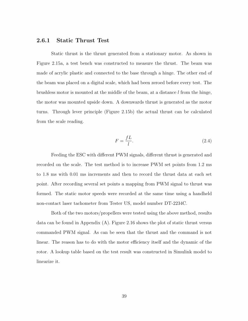
2.6.1 Static Thrust Test
Static thrust is the thrust generated from a stationary motor. As shown in
Figure 2.15a, a test bench was constructed to measure the thrust. The beam was
made of acrylic plastic and connected to the base through a hinge. The other end of
the beam was placed on a digital scale, which had been zeroed before every test. The
brushless motor is mounted at the middle of the beam, at a distance l from the hinge,
the motor was mounted upside down. A downwards thrust is generated as the motor
turns. Through lever principle (Figure 2.15b) the actual thrust can be calculated
from the scale reading.
F =fL
l. (2.4)
Feeding the ESC with different PWM signals, different thrust is generated and
recorded on the scale. The test method is to increase PWM set points from 1.2 ms
to 1.8 ms with 0.01 ms increments and then to record the thrust data at each set
point. After recording several set points a mapping from PWM signal to thrust was
formed. The static motor speeds were recorded at the same time using a handheld
non-contact laser tachometer from Tester US, model number DT-2234C.
Both of the two motors/propellers were tested using the above method, results
data can be found in Appendix (A). Figure 2.16 shows the plot of static thrust versus
commanded PWM signal. As can be seen that the thrust and the command is not
linear. The reason has to do with the motor efficiency itself and the dynamic of the
rotor. A lookup table based on the test result was constructed in Simulink model to
linearize it.
39

(a)
(b)
Figure 2.15: Static thrust test bench
2.6.2 Frequency Response Test
The transfer function of the BLDC motor-ESC subsystem is derived through
measuring the frequency response of the propulsion module. A speed sensor is con-
structed using a photo diode to measure the dynamic motor speed.
2.6.2.1 Motor Speed sensor
One of the most popular devices to measure dynamic motor speed is the optical
encoder. The usual way to use the encoder is to mount the coding disk to the motor
shaft so that the disk will rotate synchronously with the shaft (Figure 2.17a). Motor
position is measured by counting the pulses and velocity is derived (Figure 2.17b).
40

(a) Thrust of Motor A
(b) Thrust of Motor B
Figure 2.16: Static thrust test plot of two motors
However, such assembly configuration is not suitable for the brushless motors
used here due to the propeller installation that takes the entire shaft. Alternatively
a Hall effect sensor is widely used to detect rotor position in many brushless motors
by generating pulses for the rotating magnets. In this case the rotor of the BLDC
motor is the external case that has magnets fixed inside. The motor case blocks the
internal magnetic field thus renders the switching magnetic pole undetectable by the
Hall-effect sensor from outside. Also due to its compact design, there is no way to
mount a sensor inside to detect the switching coils.
An encoder-like speed sensor was designed using photo diodes to measure the
41

(a) optical encoder coding disk assembly
(b) Optical generated pulses
Figure 2.17: Optical encoder
dynamic motor speed. As shown in Figure 2.18, the surface of the case was converted
to create alternating absorbtive and reflective surfaces using acrylic glass protective
film. In order to suppress the interference of visible light, infrared LED emitters and
infrared diodes were used. The LED and photo diode were fixed relative to the motor
housing. They are arranged at such an angle that the reflection of the LED from the
motor case can be mostly received by the diode. When the motor case spins with the
shaft, the level of reflection changes from the diode’s aspect.
Variation in the reflection causes the voltage of the diode to change when it
is connected in a circuit. The voltage is then compared with a reference voltage in
an operational amplifier (Figure 2.19). At the moment a grid is turning past the
42

Figure 2.18: Speed sensor configuration
LED, a pulse is generated at the circuit’s output when the diode’s voltage is higher
than the reference voltage. The pulse is sent to the Q8 board’s encoder input and
the number of pulses is counted in the encoder chip. Just like the encoder’s coding
disk, the more grids cut on the film the higher the resolution of the sensor. However
there is a minimum area required by the diode to generate enough voltage difference
to create a change between reflective and non-reflective windows. In the proposed
design, twenty windows are cut on the low reflection film.
Figure 2.19: infrared diode circuit
43

2.6.2.2 Frequency Response
The ESC-motor system is assumed to be a first order system with a communi-
cation delay of Td seconds. Td is selected as 5 milliseconds, and the transfer function
is assumed to be
G(s) =1
Ts+ 1e−Tds. (2.5)
After mounted with a propeller, the motor is commanded to track a desired
sinusoidal speed with different frequencies. Frequencies were selected from 0.25 Hz to
1 Hz with increments of 0.25, from 1 Hz to 3 Hz with increments of 0.1, and from 3 Hz
to 8 Hz with increments of 1. The resulting motor speeds were recorded. As shown
in Figure 2.20, the accelerating parts and decelerating parts are not symmetric. This
is due to the aerodynamic drag of the propeller and the ESC not applying braking
while it commands the motor to slow. The temporal displacement between desired
speeds and actual speeds are measured.
Figure 2.20: Plot of desired speed and actual speed at frequency 0.75 Hz
A bode phase plot is formed by plotting all the measured phase shift data in
degrees and the corresponding frequencies in radians/s (Figure 2.21). From the Bode
phase plot, T can be estimated as 0.113 seconds. Therefore the ESC-motor system
44

transfer function is identified as:
G(s) =1
0.113s+ 1e−0.005s. (2.6)
Figure 2.21: Bode phase plot of ESC-motor system
To improve the overall system performance, it is desired for the propulsion
module to have a large phase margin. A compensator can partially improve the
subsystem frequency response. Based on Equation (2.6), a Phase Lead Compensator
(2.22) is designed to reshape the frequency response.
G(s) =s+ pos+ pn
(2.7)
As shown in Figure 2.22 the compensator pulls the pole of the uncompensated
system further away from the imaginary axis to pn, resulting in higher phase margin.
45
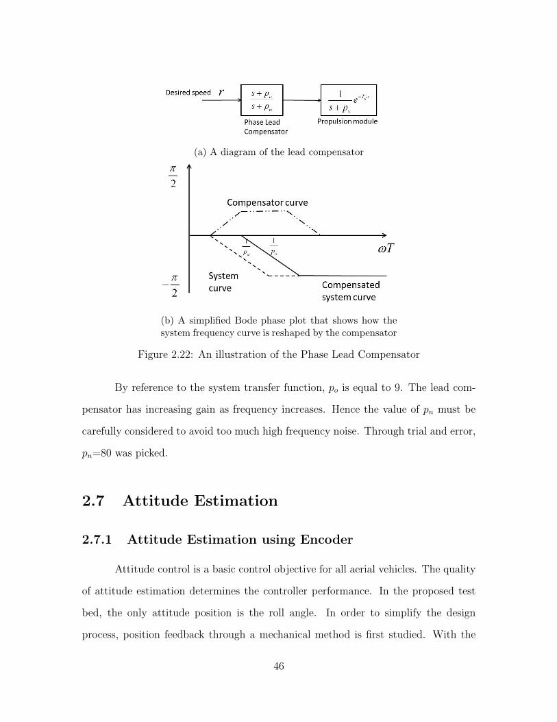
(a) A diagram of the lead compensator
(b) A simplified Bode phase plot that shows how thesystem frequency curve is reshaped by the compensator
Figure 2.22: An illustration of the Phase Lead Compensator
By reference to the system transfer function, po is equal to 9. The lead com-
pensator has increasing gain as frequency increases. Hence the value of pn must be
carefully considered to avoid too much high frequency noise. Through trial and error,
pn=80 was picked.
2.7 Attitude Estimation
2.7.1 Attitude Estimation using Encoder
Attitude control is a basic control objective for all aerial vehicles. The quality
of attitude estimation determines the controller performance. In the proposed test
bed, the only attitude position is the roll angle. In order to simplify the design
process, position feedback through a mechanical method is first studied. With the
46

constraint of the tether, evaluating the rolling motion of the 2D MOVA can be viewed
as measuring the rotary joint where the UAV attaches to the tether. It is desired
to use an optical encoder to measure angle, first and second differentiation of the
measurement provides an estimate of the angular rates and accelerations.
The roll angle change of the 2D MOVA is very little. Given that the control
algorithms are dependent on attitude feedback of high accuracy, an encoder with
acceptable resolution is required. Since the encoder will be mounted on-board or fixed
with the tether linkage, it will work under the influence of vibration which is produced
from the propulsion unit. The encoder should provide reasonable measurements that
support the estimation of the velocity and acceleration. After careful consideration,
the TRD-S2500 quadrature encoder provided by Koyo was selected. It provides a
resolution of 2500 pulses per revolution, requires 5V DC input. The encoder body
is 1.5 inches diameter and 1.6 inches depth and weights 42 grams thus is compact
enough to put onboard.
2.7.1.1 Gear Design to transmit rotary motion
Due to the limited space on the airframe, the encoder is designed to mount on
the tether linkage. As shown in Figure 2.23, a clamp is constructed by two pieces of
acrylic plastic to secure the encoder bracket.
47
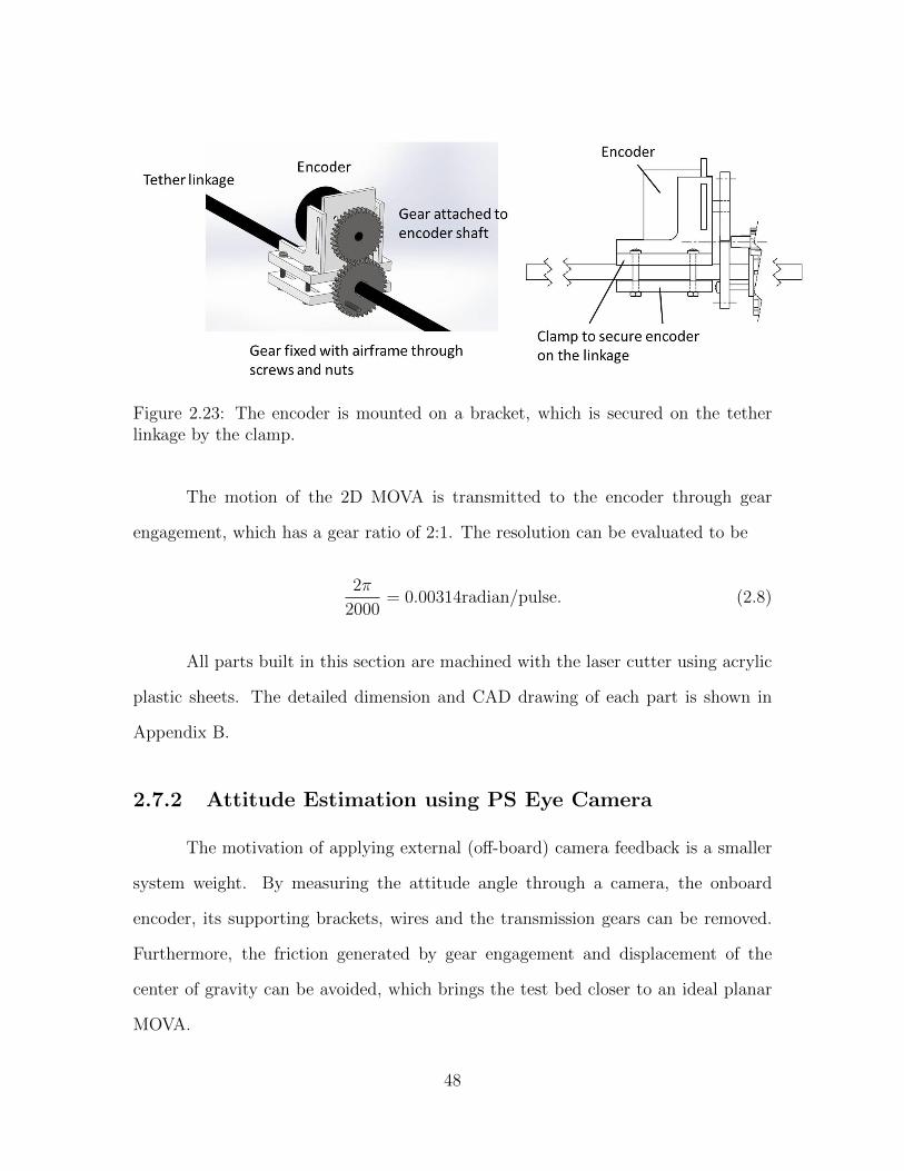
Figure 2.23: The encoder is mounted on a bracket, which is secured on the tetherlinkage by the clamp.
The motion of the 2D MOVA is transmitted to the encoder through gear
engagement, which has a gear ratio of 2:1. The resolution can be evaluated to be
2π
2000= 0.00314radian/pulse. (2.8)
All parts built in this section are machined with the laser cutter using acrylic
plastic sheets. The detailed dimension and CAD drawing of each part is shown in
Appendix B.
2.7.2 Attitude Estimation using PS Eye Camera
The motivation of applying external (off-board) camera feedback is a smaller
system weight. By measuring the attitude angle through a camera, the onboard
encoder, its supporting brackets, wires and the transmission gears can be removed.
Furthermore, the friction generated by gear engagement and displacement of the
center of gravity can be avoided, which brings the test bed closer to an ideal planar
MOVA.
48
2.7.2.1 Camera Setup
The sensor of the vision feedback system is required to provide adequate res-
olution and update rate. A PlayStation R©Eye (also referred to as PS Eye) digital
camera was selected as the sensor. The PS Eye camera was first designed as a gesture
recognition sensor for the PlayStation 3 game console, so that the player can interact
with the games by their motions and gestures. The camera has two resolution modes:
VGA with a resolution of 640 x 480 pixels, and QVGA (Quarter-VGA), 320 x 240
pixels. The update rate under VGA mode is 75 frames per second, and QVGA 125
frames per second.
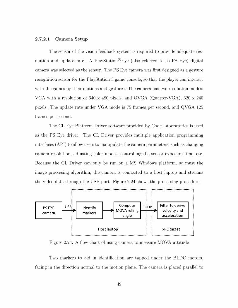
The CL Eye Platform Driver software provided by Code Laboratories is used
as the PS Eye driver. The CL Driver provides multiple application programming
interfaces (API) to allow users to manipulate the camera parameters, such as changing
camera resolution, adjusting color modes, controlling the sensor exposure time, etc.
Because the CL Driver can only be run on a MS Windows platform, so must the
image processing algorithm, the camera is connected to a host laptop and streams
the video data through the USB port. Figure 2.24 shows the processing procedure.
Figure 2.24: A flow chart of using camera to measure MOVA attitude
Two markers to aid in identification are tapped under the BLDC motors,
facing in the direction normal to the motion plane. The camera is placed parallel to
49
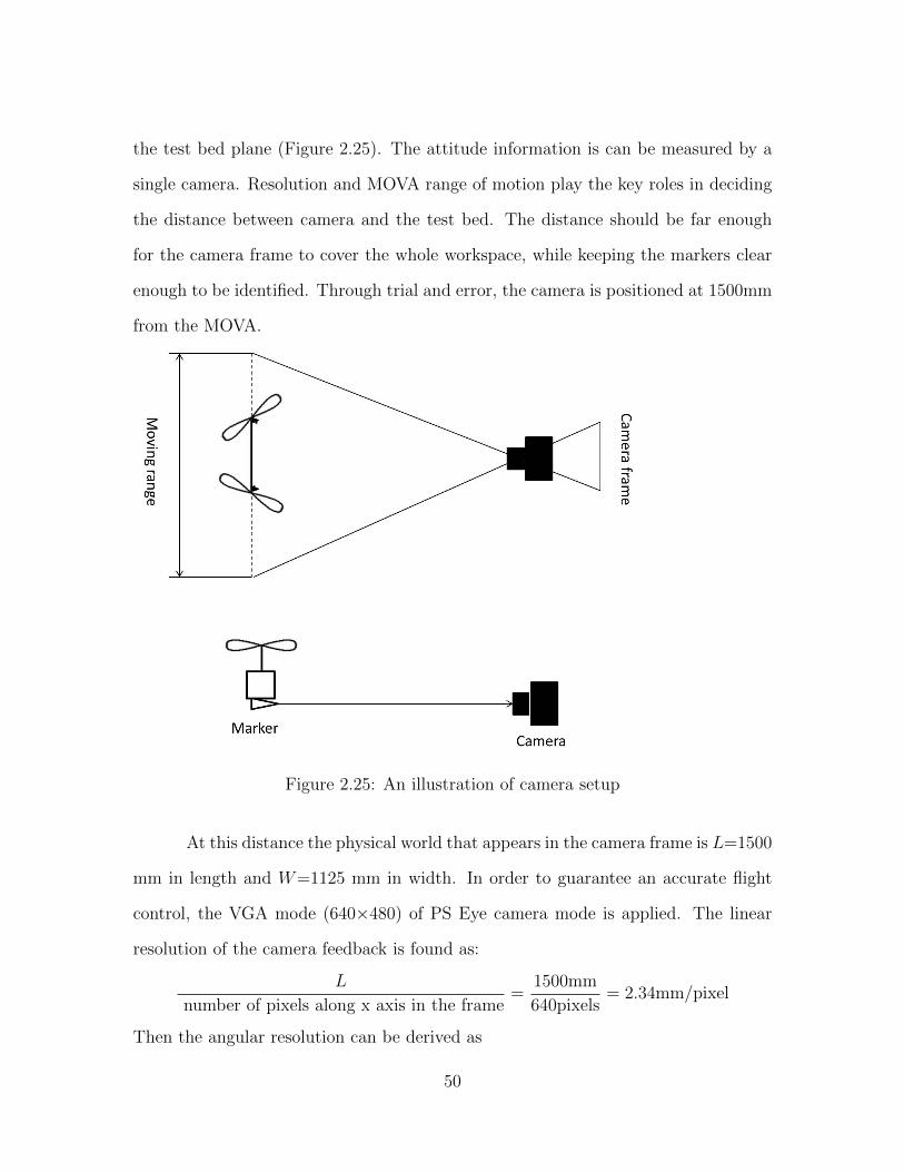
the test bed plane (Figure 2.25). The attitude information is can be measured by a
single camera. Resolution and MOVA range of motion play the key roles in deciding
the distance between camera and the test bed. The distance should be far enough
for the camera frame to cover the whole workspace, while keeping the markers clear
enough to be identified. Through trial and error, the camera is positioned at 1500mm
from the MOVA.
Figure 2.25: An illustration of camera setup
At this distance the physical world that appears in the camera frame is L=1500
mm in length and W=1125 mm in width. In order to guarantee an accurate flight
control, the VGA mode (640×480) of PS Eye camera mode is applied. The linear
resolution of the camera feedback is found as:
L
number of pixels along x axis in the frame=
1500mm
640pixels= 2.34mm/pixel
Then the angular resolution can be derived as
50

arctan(distance resolution
length of airframe) = arctan(2.34/150) = 0.0156 radian/pixel .
2.7.2.2 Image Processing Algorithm
The image processing algorithm was implemented in C++ environment. Open
Source Computer Vision Library (OpenCV) was used. OpenCV is an open source
computer vision and machine learning library. It provides many image processing
functions, such as geometric operations, morphology, feature detectors, etc.
The markers are distinguished from the background by their light intensity
therefore all the frames are first transformed from RGB to gray scale images. The
resulted frames are further transformed to binary images through image segmentation.
Erosion and dilation algorithms are called to filter out the noise in the background
image.
Two regions of connected pixels (connected components), denoting the rough
location of two markers, are identified and labeled. The center of gravity of each
region is computed to derive the exact location of the markers with respect to the
frame. The actual rotation angle of the VTOL with respect to the ground is evaluated
from the angle between the line segments marked by two markers and the x-axis in
the frame.
When the algorithm starts, the rotation angle of the first frame, which repre-
sents the VTOL original attitude position, is stored. The angles derived from frames
afterward are subtracted by the original angle to derive the current attitude position.
This way a common start point for encoder and camera measurement is provided,
which simplifies the comparison tests elaborated in the following section.
51
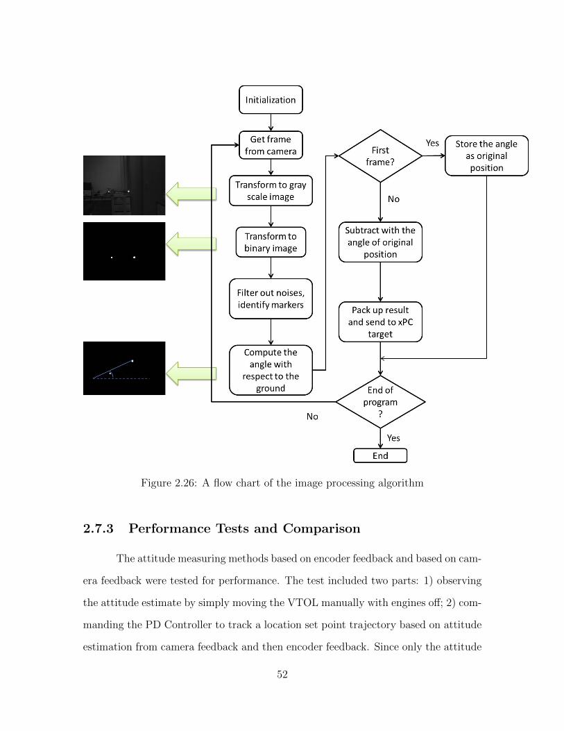
Figure 2.26: A flow chart of the image processing algorithm
2.7.3 Performance Tests and Comparison
The attitude measuring methods based on encoder feedback and based on cam-
era feedback were tested for performance. The test included two parts: 1) observing
the attitude estimate by simply moving the VTOL manually with engines off; 2) com-
manding the PD Controller to track a location set point trajectory based on attitude
estimation from camera feedback and then encoder feedback. Since only the attitude
52

positions of the host 2D VTOL aerial are evaluated and compared, the robotic arm
was removed to avoid disturbance. A simple proportional-derivative (PD) controller
is constructed to control the 2D VTOL.
2.7.3.1 PD Controller Construction
The dynamic model of the 2D MOVA is constructed by the Newtonian ap-
proach as:
mx = Fsinθ
mz +mg = Fcosθ
Jθ = τ
The system is linearized at the equilibrium point θ = 0. The linearized dynamic
function was rewritten in state space matrix form as:
m 0 0
0 m 0
0 0 J
x
z
θ
+
0
mg
0
=
Fθ
F
τ
(2.9)
As the altitude control (motion along z axis) does not involve attitude control
after linearization, the z trajectory will not be tested. A constant thrust that equals
to the VTOL gravity is applied to maintain an approximately constant altitude. With
F held constant, θ can be viewed as the control input for position control
x = kθd.
Controller computes a desire θ from errors in current position according to
53

θd = k(xr − x).
The attitude control is then achieved by computing the errors of VTOL roll angle
and angular rate
θ =Kp(θd − θ) +Kd(θd − θ)
J.
Figure 2.27 shows a schematic of the PD controller design.
Figure 2.27: Diagram of the PD Controller.
2.7.3.2 Manually Moving the VTOL
The 2D VTOL was manually moved at angles from roughly +0.3 radian to
-0.3 radian at different velocities. The results are shown in Figure 2.28.
54

(a) Encoder and camera feedback comparison
(b) A zoom in the angle measuring comparison
Figure 2.28: Roll angle measurement of encoder and camera feedback from manualtest
55

Figure 2.29: A comparison of derived velocity evaluation between encoder feedbackand camera feedback
Close inspection of Figure 2.28 reveals that the feedback from camera has
around 20 ms delay compared to the encoder feedback. The latency is speculated to
include the frame update, computational time for the host PC and the data lost during
transmitting to the target PC. Figure 2.29 also demonstrates similar performances
on velocity estimation, while the encoder is relatively smoother than the camera.
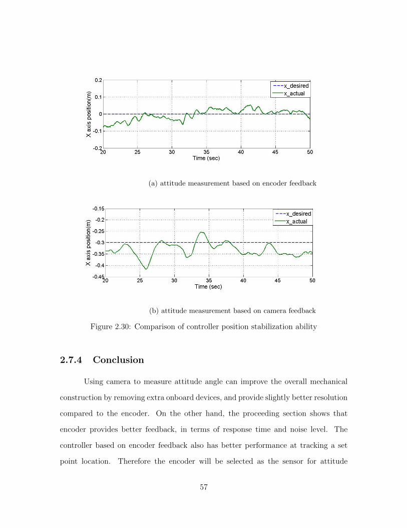
2.7.3.3 Set Point Trajectory
The set point is set at 0 mm. The 2D VTOL is commanded to stay at the
origin in the plane. The controller gain is set to k=1.3, kp=10.2 and kd=2.6. Results
are shown in Figure 2.30. The steady state errors of the system based on encoder
feedback are less than 0.08 m, while the steady error of the system based on camera
varies dramatically from +0.25 m to -0.43 m.
56
(a) attitude measurement based on encoder feedback
(b) attitude measurement based on camera feedback
Figure 2.30: Comparison of controller position stabilization ability
2.7.4 Conclusion
Using camera to measure attitude angle can improve the overall mechanical
construction by removing extra onboard devices, and provide slightly better resolution
compared to the encoder. On the other hand, the proceeding section shows that
encoder provides better feedback, in terms of response time and noise level. The
controller based on encoder feedback also has better performance at tracking a set
point location. Therefore the encoder will be selected as the sensor for attitude
57
estimation of the MOVA.
2.8 Summary
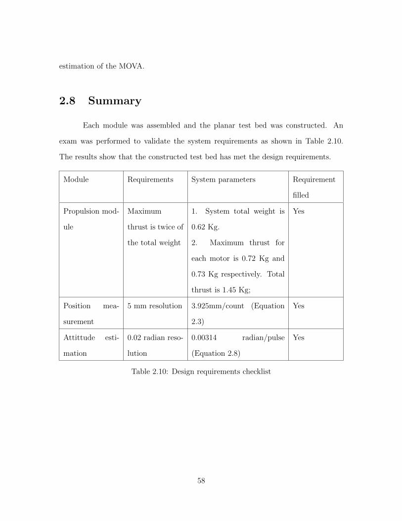
Each module was assembled and the planar test bed was constructed. An
exam was performed to validate the system requirements as shown in Table 2.10.
The results show that the constructed test bed has met the design requirements.
Module Requirements System parameters Requirement
filled
Propulsion mod-
ule
Maximum
thrust is twice of
the total weight
1. System total weight is
0.62 Kg.
2. Maximum thrust for
each motor is 0.72 Kg and
0.73 Kg respectively. Total
thrust is 1.45 Kg;
Yes
Position mea-
surement
5 mm resolution 3.925mm/count (Equation
2.3)
Yes
Attittude esti-
mation
0.02 radian reso-
lution
0.00314 radian/pulse
(Equation 2.8)
Yes
Table 2.10: Design requirements checklist
58
Chapter 3
Experiments and Results
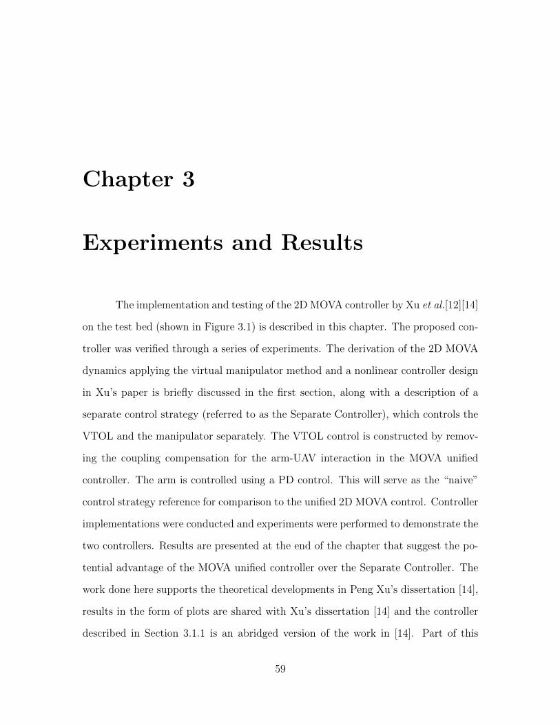
The implementation and testing of the 2D MOVA controller by Xu et al.[12][14]
on the test bed (shown in Figure 3.1) is described in this chapter. The proposed con-
troller was verified through a series of experiments. The derivation of the 2D MOVA
dynamics applying the virtual manipulator method and a nonlinear controller design
in Xu’s paper is briefly discussed in the first section, along with a description of a
separate control strategy (referred to as the Separate Controller), which controls the
VTOL and the manipulator separately. The VTOL control is constructed by remov-
ing the coupling compensation for the arm-UAV interaction in the MOVA unified
controller. The arm is controlled using a PD control. This will serve as the “naive”
control strategy reference for comparison to the unified 2D MOVA control. Controller
implementations were conducted and experiments were performed to demonstrate the
two controllers. Results are presented at the end of the chapter that suggest the po-
tential advantage of the MOVA unified controller over the Separate Controller. The
work done here supports the theoretical developments in Peng Xu’s dissertation [14],
results in the form of plots are shared with Xu’s dissertation [14] and the controller
described in Section 3.1.1 is an abridged version of the work in [14]. Part of this
59
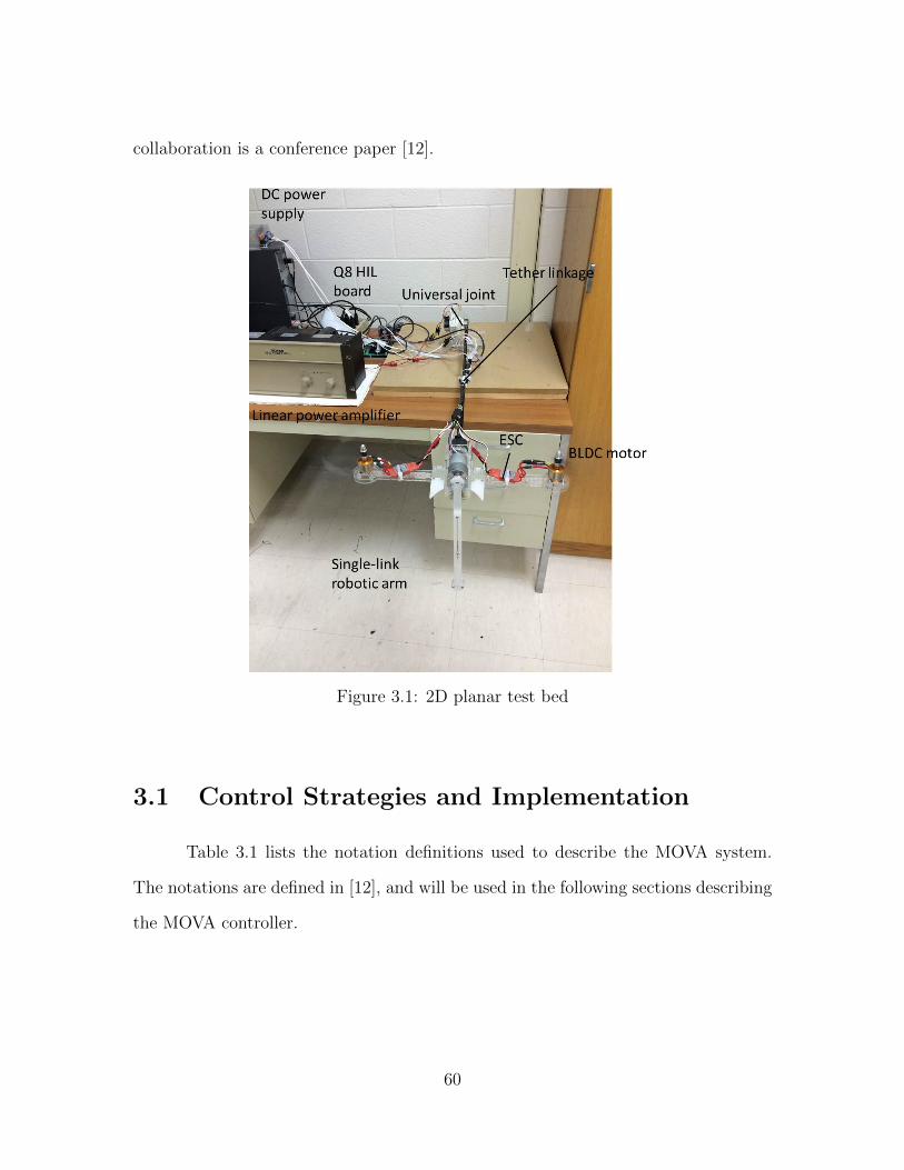
collaboration is a conference paper [12].
Figure 3.1: 2D planar test bed
3.1 Control Strategies and Implementation
Table 3.1 lists the notation definitions used to describe the MOVA system.
The notations are defined in [12], and will be used in the following sections describing
the MOVA controller.
60

Symbol Descriptionm0 mass of the VTOL aircraftJ0 moment of inertia of the VTOL aircraftm1 mass of the single manipulator linkJ1 moment of inertia of the dummy robotic arm about its
rotation axismT The total mass of the VTOL aircraft and the manipu-
latorl1 length of the dummy robotic armpe vector of coordinates of the end-effectorθ0 attitude angle of the VTOL aircraftθ1 angle between the VTOL and the armθ01 short notation of θ0 + θ1F body-fixed thrust force generated by the VTOL aircraftτ0 external torque on the body of the VTOL aircraftτ1 torque driving the single-link manipulator
Table 3.1: Notation description
3.1.1 MOVA Dynamics Derivation and Control Design
3.1.1.1 Dynamics Derivation
The MOVA dynamics derivation in this section involves two key concepts–the
virtual ground and the virtual manipulator. The virtual ground represents the center
of mass of the whole system. The coordinate of the virtual ground in the inertia
frame can be found for the planar MOVA case as
pvg =N∑i=0
mipi
=1
mT
(m0p0 +m1p1)
= p0 +l1m1
2mT
cosθ01sinθ01
.(3.1)
61

The virtual manipulator can be viewed as series of carefully chosen vectors that start
from the virtual ground and end at the exact same end-effector position and with
same orientation of the real manipulator. One advantage of the virtual ground and
the virtual manipulator over conventional kinematic methods, which starts from the
VTOL body to describe the position of end-effector, is that they are immune to the
internal torque and force and thus can be viewed as two separate systems. Following
the derivation steps, the position of the end-effector can be written as:
pe = pvg +l1(mT +m0)
2mT
cosθ01sinθ01
(3.2)
and
pe = pvg + V1 + V2
= pvg +l1(mT +m0)
2mT
cosθ01sinθ01
. (3.3)
The detailed derivation process of the virtual ground and virtual manipulator can be
found in [14].
The dynamics of MOVA system are derived though a Lagrangian approach,
and put into the form
M(q)q + C(q, q)q +G(q) = τ. (3.4)
62

The complete matrices of Equation (3.4) are given by:
M =
mT 0 −12l1m1sinθ01 −1
2l1m1sinθ01
0 mT12l1m1cosθ01
12l1m1cosθ01
−12l1m1sinθ01
12l1m1cosθ01 J0 + J1 +
l21m1
4J1 +
l21m1
4
−12l1m1sinθ01
12l1m1cosθ01 J1 +
l21m1
4J1 +
l21m1
4
, (3.5)
C =
0 0 −12l1m1cosθ01θ01 −1
2l1m1cosθ01θ01
0 0 −12l1m1sinθ01θ01 −1
2l1m1sinθ01θ01
0 0 0 0
0 0 0 0
, (3.6)
G =
[0 mTg
12l1m1cosθ01g
12l1m1cosθ01g
]T, (3.7)
τ =
[−Fsinθ0 Fcosθ0 τ0 τ1
]T. (3.8)
The dynamic equation clearly shows the off-diagonal terms in M(q) and C(q, q),
which represent the interaction between the onboard manipulator and the VTOL. By
applying the virtual manipulator method, the dynamics equation can be rewritten
in a more concise form where the virtual ground and the virtual manipulator can be
viewed as two separate systems and to facilitate the control design. The decoupled
dynamics equation can be found by:
mT pvg +
0
mTg
=
−Fsinθ0Fcosθ0
, (3.9)
63

J0θ0 = τ0 − τ1, (3.10)
and
J1θ01 = τ1 − ξ1F, (3.11)
where J1 = J1 +l1m0m1
4mT
and ξ1 =l1m1
2mT
cosθ1.
3.1.1.2 Control Design
The objective is to design a controller to follow the desired end-effector trajec-
tory per(t) and θer(t). The subscript “r”” denotes a reference version of the variable.
By adopting back-stepping technique, a Lyapunov-based nonlinear controller can be
derived. The design process can be divided into two parts: virtual ground control
design, forcing the virtual ground position pvg to track the desired position pvgr;
and virtual manipulator design, directing the end-effector angle θe01 to converge to a
reference angle θe01r
Virtual ground control. A filtered tracking error is first defined as
r = ev + αep + δ, (3.12)
where α ∈ R+ and δ = [0, δ2]T are control gains. evand ep are filtered tracking errors
which are given by
ep = RT (pvg − pvgr), (3.13)
and
ev = RT ( ˙pvg − ˙pvgr), (3.14)
64

R transforms a vector in the inertial frame into VTOL body frame
R =
cosθ0 −sinθ0sinθ0 cosθ0
, (3.15)
r can be found by taking time derivative of Equation (3.12). The equation for the
r-dynamics clearly shows the control input
r = S(ω)r + αev −RT (pvgr + gv) +
−δ2 0
0 m−1T
·ωF
= S(ω)r + ξ2 +Bµµ,
(3.16)
The above equation is then organized in a more concise form
r = S(ω)r + ξ2 +Bµµ, (3.17)
where ξ2 = αev −RT ( ¨pvgr + gv) and
Bµ =
−δ2 0
0 m−1T
, and µ =
ωF
, (3.18)
Among the two control inputs, F can be directly controlled by motor thrust, while
ω is the output of the θ0 dynamics. A typical back-stepping technique is applied by
injecting a tracking error in Equation (3.17) to yield
r = S(ω)r + ξ2 +Bµ(µd + µe), (3.19)
65

where
µe =
ωeFe
= µ− µd =
ω − ωdF − Fd
. (3.20)
To regulate r, µd is designed as
µd =
ωdFd
= B−1µ (−krr − ξ2 − ep). (3.21)
The control inputs should push the tracking errors to approach 0. It is clear that
F = Fd =
[0 1
]µd. (3.22)
While the dynamics of θ0 is controlled by the net torque applied on VTOL τn, which
equals to τ0 − τ1, as shown in Equation (3.23)
J0ωe = J0θ0 −[J0 0
]µd
= τn −[J0 0
]µd.
(3.23)
τn is revealed by referencing the Lyapunov stability analysis [15] as
τn = −kωJ0ωe +
[J0 0
]µd +
[δ2 0
]r. (3.24)
End-effector orientation control. Similar to the virtual ground control, a
filtered orientation tracking error is formulated as
r2 = ˙e01 + βe01 (3.25)
where β is the control gain and e01 is the error between the actual end-effector orien-
66

tation and the reference orientation, which can be expressed as
e01 = θ01 − θ01r (3.26)
and
e01 = θ01 − θ01r. (3.27)
The control input of θ01, τ1 can be introduced into the tracking error r2 dynamics
by taking time derivative of Equation (3.25) and multiplying J1 on both side of the
equation
J1r2 = J1θ01r + J1βe01
= τ1 − ξ1F − J1(θ01r − βe01),(3.28)
τ1 is then specified as
τ1 = −k2J1r2 + ξ1F + J1(θ01r − βe01 − e01). (3.29)
The external torque applied on the VTOL is revealed to be the sum of τn and τ1
τ0 = τn + τ1, (3.30)
At this the point, three control inputs to the planar MOVA system have been specified
in Equation (3.22), (3.29) and (3.30).
3.1.2 Separate Control Strategy
The Separate Controller has two separate parts–VTOL control and end-effector
control. The VTOL control strategy is constructed following the exact same design
67

steps as the virtual ground control of the planar MOVA, but based solely on the
dynamics of a planar VTOL (Equation (2.9)). Simply put, replace the virtual ground
coordinate and reference virtual ground trajectory everywhere in the MOVA dynam-
ics with the VTOL body coordinate and the reference VTOL body trajectory. The
external thrust input can be found by Equation (3.22), replacing the reference virtual
ground acceleration pvgr with the reference VTOL body acceleration p0r in µd. The
modified µd is written as
µd =
ωdFd
= B−1µ (RTgv + p0r − αev − ep− krr). (3.31)
The control input thrust F is
F =
[0 1
]ωdFd
= B−1µ (RTgv + p0r − αev − ep− krr). (3.32)
Same process applies for finding the external torque on the VTOL τ
τ = −kωJ0ω0e +
[J0 0
]µ0d +
[δ2 0
]r0, (3.33)
where ω0e,µ0d and r0 are the VTOL body version of the corresponding variables.
The end-effector control applies a typical PD controller, which tracks desired
rotation angles with respect to the VTOL. Note that the desired inputs from the
user are the end-effector position Per and the end-effector direction θer, with respect
to the inertial frame. While the input to the separate controller is the position and
attitude angle, which are denoted as pr and θ0r. Therefore the input coordinate to
the separate system must first be transformed to a VTOL coordinate before being
68

sent to the Separate Controller.
3.1.3 Controller Implementation
Both of the systems were implemented through Simulink models and executed
by an xPC Target workstation through the Q8 HIL board. The Q8 board was set
at a sampling rate of 100 Hz. Note that the MOVA control input to the on-board
manipulator is torque computed by the control algorithm while the DC motor that
drives the manipulator requires voltage input. The desired voltage output can be
computed by referencing to the DC motor voltage equation
Vm = Eb +RmIa. (3.34)
The notation definitions in the equations can be found in Table 3.2. Eb and Ia can
be derived from
Eb = ke ˙theta1, (3.35)
and
Ia =τ1kT, (3.36)
where ke is the motor back emf constant and kT is the torque constant. An equation
involving the manipulator angular speed and input voltage is derived by injecting
Equations (3.35) and (3.36) into Equation (3.34) to yield
Vm = keθ1 +Rmτ1kT. (3.37)
Values in Table 2.9 were assigned to the corresponding variables in Equation (3.37)
and computed for ke = 0.07 Vs/rad and Rm = 2.4Ω. Note that kT =ke2π
= 0.01
69
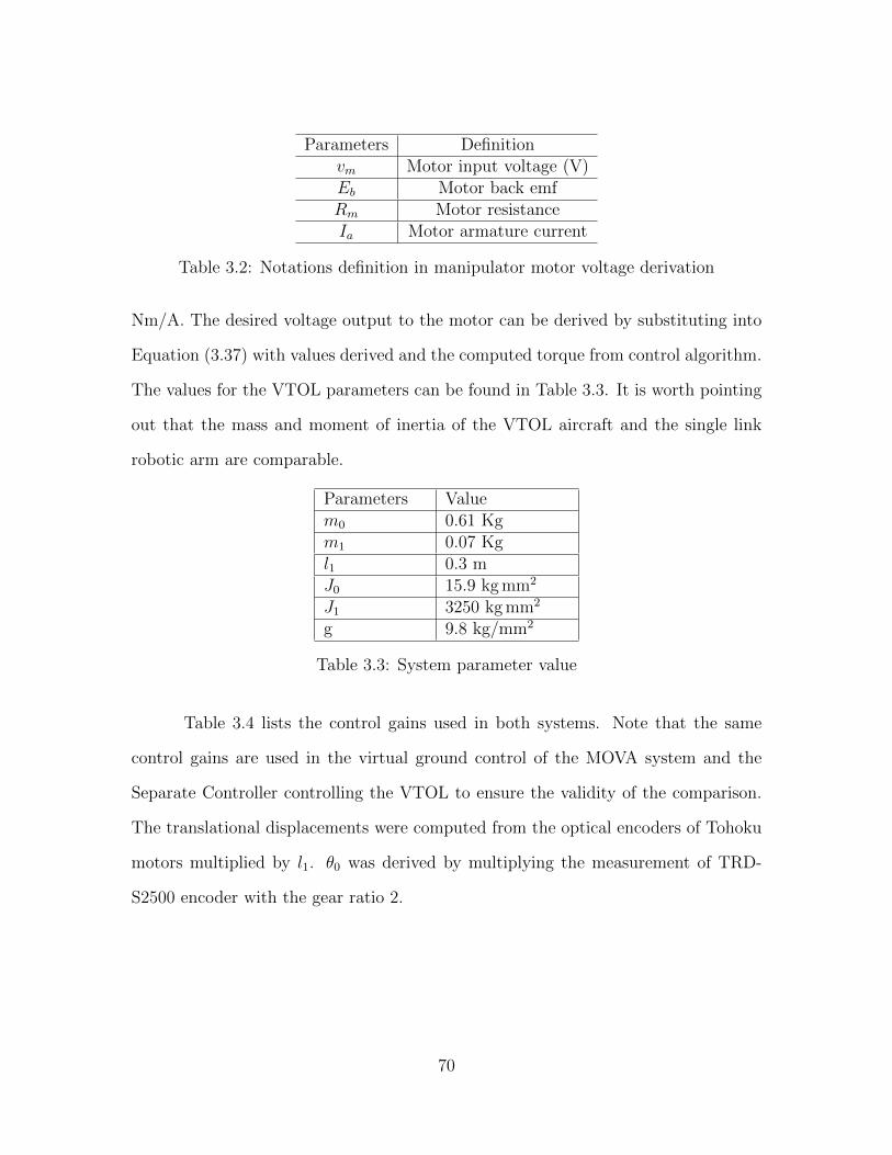
Parameters Definitionvm Motor input voltage (V)Eb Motor back emfRm Motor resistanceIa Motor armature current
Table 3.2: Notations definition in manipulator motor voltage derivation
Nm/A. The desired voltage output to the motor can be derived by substituting into
Equation (3.37) with values derived and the computed torque from control algorithm.
The values for the VTOL parameters can be found in Table 3.3. It is worth pointing
out that the mass and moment of inertia of the VTOL aircraft and the single link
robotic arm are comparable.
Parameters Valuem0 0.61 Kgm1 0.07 Kgl1 0.3 mJ0 15.9 kg mm2
J1 3250 kg mm2
g 9.8 kg/mm2
Table 3.3: System parameter value
Table 3.4 lists the control gains used in both systems. Note that the same
control gains are used in the virtual ground control of the MOVA system and the
Separate Controller controlling the VTOL to ensure the validity of the comparison.
The translational displacements were computed from the optical encoders of Tohoku
motors multiplied by l1. θ0 was derived by multiplying the measurement of TRD-
S2500 encoder with the gear ratio 2.
70

Gains Valuekr 0.08kω 0.06α 1δ2 1.1β 13k2 94P (propotional gain) 10D (derivative gain) 0.1
Table 3.4: Value of control gains
3.2 Experiments and Results
In order to evaluate the planar MOVA controller, three experiments were con-
ducted, and the performance compared with the Separate Controller. The first ex-
periment was designed to test the hovering stability of the MOVA. The system initial
states were set to
[xe ze θ01
]T=
[0 −0.3 −π
2
]T. Specifically the initial attitude
of VTOL and the initial attitude of manipulator were θ0 = 0 and θ1 = −pi2
, re-
spectively. The desired trajectory was to hover at the same location and manipulate
orientation. The MOVA results are compared with the results of the Separate Con-
troller in Figure 3.2. The system was hand held until the motors reach the desired
speed because the differential response time of the two motors may lead to sudden
attitude change when taking off. The data period displayed was carefully selected to
present the largest error that appeared during the whole testing cycle. The same rule
applies for the other tests.
71

(a) x-axis of Separate Controller (b) x-axis of MOVA
(c) z-axis of Separate Controller (d) z-axis of MOVA
(e) θe of Separate Controller (f) θe of MOVA
Figure 3.2: Experiment 1, VTOL aircraft hovered at initial position
The second experiment is for the end-effector to track a desired trajectory
while the VTOL hovers. The reference trajectory mimics a pendulum motion with
range of 0.8 − π
2radian to −0.8 − π
2radian while the host VTOL stays at a fixed
72
position defined as
per =
0
0
mm. (3.38)
The desired end-effector position trajectory and direction are defined as
θ01r(t) = 0.8sin(1.5t)− π
2
Per =
l1cosθ01rtl1sinθ01rt
. (3.39)
The experimental results are reported in Figure 3.3.
73

(a) x-axis of Separate Controller (b) x-axis of MOVA
(c) z-axis of Separate Controller (d) z-axis of MOVA
(e) θe of Separate Controller (f) θe of MOVA
Figure 3.3: Experiment 2, tracking pendulum motion trajectory
74

In the third experiment a reference trajectory of inverted pendulum motion
was input to the system, which is defined as:
Per =
0
−0.25
m
θ01r(t) = 0.8sin(1.5t)− π
2.
(3.40)
It is analogous to fastening a hexagon head bolt with a ratcheting wrench
that the simulated robotic arm is a wrench operated by the VTOL (Figure 3.4).
The trajectory is more difficult to perform in terms of the throttle control. The test
evaluates the accuracy of the static thrust mapping in Chapter 2. Figure 3.5 presents
the results.
Figure 3.4: An illustration of the “wrenching a bolt” trajectory
75

(a) x-axis of Separate Controller (b) x-axis of MOVA
(c) z-axis of Separate Controller (d) z-axis of MOVA
(e) θe of Separate Controller (f) θe of MOVA
Figure 3.5: Experiment 3, tracking inverted pendulum motion trajectory
76
3.3 Summary
In the first experiment, tracking a fixed location, the behavior of both systems
are similar. Errors of xe both remain below 5 centimeters, while the position errors
projected to the z- axis have a constant error of about 0.05 m. It is partially due to
the deteriorating performance of the motors after constantly running at full throttle
for a long period of time.
In Experiment 2, a sinusoidal pattern was formed in the Separate Controller
actual position projected to the x- axis, which results in fluctuating errors in the
range from 0 m to 0.2 m. The errors may relate to the disturbance introduced by the
manipulator to the system. The VTOL was “dragged” away by the shifted center of
gravity of the manipulator and was only able to correct the position passively. On the
other hand, active attitude changes of host VTOL were observed in MOVA system.
The moves partially cancel out the systems internal torque, demonstrating the active
compensation for interaction between manipulator and VTOL. The MOVA showed
satisfying performance by keeping the xe errors within 0.1 m. The results strengthen
the claim that the planar MOVA controller takes into account the interactions between
manipulator and the VTOL aerial vehicle.
In Experiment 3, the θ01 errors in both system are small as in the preceding
tests. But the MOVA position tracking errors had seemingly increased. This can be
improved by refining mapping from ESC PWM signal to the static thrust, or further
designing a throttle controller based on propeller aerodynamics.
77

Chapter 4
Conclusions
A planar test bed, which consists of an instrumented tether and an experi-
mental, 3 DOF planar UAV and single-link manipulator system, for UAV controller
evaluation was presented in this thesis. A recently designed unified controller of a
Manipulator On the VTOL Aircraft (MOVA) was validated. The test bed design
process followed the top-down functional decomposition method. All components of
the test bed were described and necessary details for replicating the test bed were
provided. The propulsion modules were characterized based on the results of the
frequency response tests. Two methods of VTOL attitude measurement, the en-
coder mechanical feedback via the tether and camera vision feedback, were explored.
Performance tests were conducted on the test bed using both methods of feedback
and the encoder was determined to be a better choice of sensor due to the better
performance in this specific system.
The MOVA dynamics derivation based on the virtual manipulator method
and the unified controller was briefly discussed. A modified controller, referred to
as the Separate Controller, which removes the coupling compensation for the arm-
UAV interaction, was designed for performance comparison. Both the MOVA system
78

and the Separate Controller were validated through experiments and the results were
compared. The tests on the Separate Controller showed the negative impact of manip-
ulator interaction on VTOL flying trajectory when tracking a reference end-effector
trajectory. The MOVA unified controller, on the other hand, was able to actively
compensate for the interaction and provided more refined tracking motion.
In summary, the test bed design met the need to produce a physical demon-
stration of the 2D MOVA controller. The instrumented tether can be used with
other VTOL aircraft and the test bed as a whole can be used to test other control
algorithms.
The system performance could be improved by replacing the components sug-
gested in Table 4.1 to reduce the overall weight. Future research can be directed on
developing a manipulator with grasping function and studying adaptive control de-
sign techniques to automatically tune the system parameters when the manipulator
is interacting with other objects.
Current components ReplacementTRD-S2500 Optical encoder Triple axis gyroscope [18]
Hollow fiberglass tube in tether Carbon fiber tube [23]Ball bearings that connect the airframe and the tether Ball bearing guide bushing [20]
Table 4.1: Recommended components
79

Appendices
80

Appendix A Results of Static Thrust Test
Motor AThrust (gram) Speed
(r/s)PWMduty cycle(ms)
Thrust (gram) Speed(r/s)
PWMduty cycle(ms)
20.27719 36 1.2 395.6524 89 1.4840.05981 41 1.22 417.166 91 1.4960.83156 45 1.24 436.2068 93 1.584.07614 48 1.26 450.7965 96 1.51107.568 51 1.28 469.8372 98 1.52129.3289 56 1.3 489.6199 101 1.53142.1876 62 1.31 501.984 103 1.54154.5517 64 1.32 521.7666 104 1.55164.443 65 1.33 541.5492 107 1.56176.8072 66 1.34 556.3862 108 1.57189.6659 67 1.35 578.6417 110 1.58200.0518 68 1.36 593.4786 113 1.59211.9213 71 1.37 610.7884 115 1.6226.7583 72 1.38 620.6797 116 1.61237.1442 74 1.39 637.9895 118 1.62247.2828 75 1.4 655.2993 120 1.63263.1089 77 1.41 665.1906 121 1.64276.9567 78 1.42 692.3917 123 1.65294.2665 80 1.43 712.1743 125 1.66316.5219 81 1.44 717.12 126 1.67333.8317 83 1.45 741.8483 129 1.68356.0872 85 1.46 744.3211 129 1.69375.8698 87 1.47
Table 2: Static thrust test results for motor A
81

Motor BThrust (gram) Speed
(r/s)PWMduty cycle(ms)
Thrust (gram) Speed(r/s)
PWMduty cycle(ms)
16.81523 35 1.2 393.1796 89 1.4835.60872 40 1.22 415.435 91 1.4954.64949 44 1.24 435.2177 92 1.577.89407 47 1.26 452.5274 94 1.5198.9131 50 1.28 472.3101 99 1.52122.8995 56 1.3 492.0927 101 1.53134.7691 59 1.31 504.4568 103 1.54149.1115 62 1.32 524.2394 105 1.55158.261 64 1.33 541.5492 107 1.56173.0979 66 1.34 558.859 108 1.57185.4621 67 1.35 578.6417 110 1.58196.0952 68 1.36 593.4786 113 1.59208.9539 70 1.37 610.7884 115 1.6222.5545 72 1.38 623.1526 116 1.61229.973 73 1.39 642.9352 119 1.62243.5735 75 1.4 652.8265 120 1.63259.6469 76 1.41 672.6091 122 1.64274.4839 78 1.42 687.4461 123 1.65294.2665 80 1.43 699.8102 124 1.66314.0491 81 1.44 712.1743 125 1.67331.3589 83 1.45 731.957 128 1.68353.6143 85 1.46 741.8483 129 1.69375.8698 87 1.47
Table 3: Static thrust test results for motor B
82

Appendix B CAD Drawings of the Encoder Bracket
Figure 1: Side part of encoder bracket
Figure 2: Front part of encoder bracket
83

Figure 3: Base part of encoder bracket
Figure 4: Encoder bracket assembly drawing
84

Bibliography
[1] T.W. Danko and P.Y. Oh, “Design and Control of a Hyper-Redundant Manip-ulator for Mobile Manipulating Unmanned Aerial Vehicles,” Journal of Intelli-gent & Robotic Systems, vol. 73, no. 1, pp. 709 - 723. Jan. 2014.
[2] F. Hoffmann, N. Goddemeier, and T. Bertram,“Attitude estimation and controlof a quadrocopter,” in IEEE/RSJ Int. Conf. on Intelligent Robots and Systems,Taipei, TW, 2010, pp. 1072 1077.
[3] A.E. Jimenez-Cano, J. Martin, G. Heredia, A. Ollero, and R. Cano, “Controlof an aerial robot with multi-link arm for assembly tasks,” IEEE Int. Conf. onRobotics and Automation (ICRA), Karlsruhe, DEU, 2013, pp. 4916 - 4921.
[4] C.M. Korpela, T.W. Danko, and P.Y. Oh, (Jan 2012) “MM-UAV: Mobile Ma-nipulating Unmanned Aerial Vehicle,” Journal of Intelligent & Robotic Systems,vol. 65, no. 1, pp. 93 101.
[5] M. Lungu and R. Lungu, “Adaptive backstepping flight control for a miniUAV,”Int. Journal of Adaptive Control and Signal Processing, vol. 27, no. 8, pp. 635- 650.
[6] N. Michael, D. Mellinger, Q. Lindsey, and V. Kumar, “The GRASP MultipleMicro-UAV Testbed,” IEEE Robot. Automat. Mag., vol. 17, no. 3, pp. 56 - 65.
[7] C. Nicol,, C.J.B. Macnab, and A. Ramirez-Serrano, . “Robust adaptive controlof a quadrotor helicopter,” in Mechatronics, 2011, vol. 21, pp.927 - 938.
[8] P.E.I. Pounds, D.R. Bersak, and A.M. Dollar, “Grasping From the Air: Hover-ing Capture and Load Stability,” in IEEE Int. Conf. on Robotics and Automa-tion. 2011, pp. 2491 - 2498.
[9] A. Tayebi and S. McGilvray, “Attitude stabilization of a VTOL quadrotor air-craft,” in IEEE Transactions on Control Systems Technology, 2006, vol. 14,no. 3, pp. 562 571.
[10] X. Wu, Y. Liu, J. Zhu, “Design and real time testing of a trajectory linearizationflight controller for the “Quanser UFO”,” in Proc. IEEE American ControlConference, Mar. 2003, Vol. 5, pp. 3913 - 3918.
85

[11] YS. Yu and XL. Ding, “A Quadrotor Test Bench for Six Degree of FreedomFlight,” Journal of Intelligent & Robotics System, vol. 68, no. 3-4, pp. 323 338,Dec. 2012.
[12] P. Xu, R. Huang, D. Lee, and T. Burg, “Dynamics and Control of a NovelMOVA System - A Planar Case Study,” in Proc. IEEE American Control Con-ference, 2014.
[13] D. Lee, C. Nataraj, T. Burg, and D. Dawson, “Adaptive Tracking Control of anUnderactuated Aerial Vehicle,” in Proc. IEEE American Control Conference,2011, pp. 2326 - 2331.
[14] P. Xu, “Unified Dynamics and Control of a Robot Manipulator Mounted ona VTOL Aircraft Platform,” Ph.D. dissertation, Dept. Elect. Eng., ClemsonUniv., Clemson, SC. 2014.
[15] S. K. Y. Nikravesh, Nonlinear systems stability analysis: Lyapunov-based ap-proach. CRC Press, 2013.
[16] LAAS-CNRS. (2003) [Online; accessed July 2014]. Available: http://homepages.laas.fr/matthieu/robots/h2bis.shtml
[17] Oscar. (2013, October). How to choose Motor and Propeller for Quadcopterand Multicopter. [Online]. Available: http://blog.oscarliang.net/how-to-choose-motor-and-propeller-for-quadcopter/
[18] Sparkfun Electron. (2014) Triple-Axis Digital-Output Gyro. [Online; accessedMay 2014]. Available: https://www.sparkfun.com/products/11977
[19] HobbyKing. (2014) Carbon fiber tube. [Online; accessed July 2014]. Available:http://hobbyking.com/hobbyking/store/__43706__Carbon_Fiber_Tube_hollow_3x2x750mm_USA_warehouse_.html
[20] Amazon. (2013) LM 10UU Linear bearing ball bushing. [On-line; accessed June 2014]. Available: http://www.amazon.com/LM10UU-Bearing-Bushing-Printer-MendelMax/dp/B00EO7GX42/ref=sr_1_1?ie=UTF8&qid=1406227540&sr=8-1&keywords=LM+10UU+Linear+bearing+ball+bushing
[21] Pololu. (2014) Metal gear motor. [Online; accessed July 2014]. Available:http://www.pololu.com/product/1445
[22] Wikipedia. (2014, July) Aluminum. [Online]. Available: http://en.wikipedia.org/wiki/Aluminium
86

[23] Clearwater Composites, LLC. (2014) Properties of Carbon Fiber. [Online;accessed July 2014]. Available: http://www.clearwatercomposites.com/
[24] Wikipedia. (2014, June) Poly (methyl methacrylate). [Online]. Available:http://en.wikipedia.org/wiki/Poly(methyl_methacrylate)
[25] Q. C. Inc. (2003) Q8 data acquisition system user’s guide. [Online]. Avail-able: http://www.clemson.edu/ces/crb/ece495/References/manuals/quanserq8manual.pdf
87