Embed Size (px)
Citation preview

Design and Characterization of a Small Wind Turbine
Model equipped with a Pitching System
In Partial Fulfilment of the Requirements for the degree
Master of Science in Engineering
Renewable Energy and Energy Efficiency for the MENA Region
(REMENA)
Done by
Fadi Abdulhadi
Supervised by
Prof. Dr. sc.techn. Dirk Dahlhaus
Dr. Michael Hölling
Dr. Basman El Hadidi
Kassel, 27th
Feb 2012

i
Table of Contents
List of Figues…………………………………………………………………………….iii
List of Tables…………………………………………………………………………..…v
Nomenclature…………………...………….……………………………………………vi
Acknowledgement .. …………………………………………………………………… vii
Abstract ……………………………………………………………………………….. viii
1. Introduction .................................................................................................................. 1
1.1 Statement of Purpose ......................................................................................... 1
1.2 Literature Review ............................................................................................... 2
1.3 Structure of the Thesis ....................................................................................... 3
2. Theoritical Backgroud ................................................................................................. 4
3. Wind Turbine Model ................................................................................................. 11
3.1 Specifications and Main Components ............................................................. 11
3.2 Blade ................................................................................................................ 13
3.3 Generator .......................................................................................................... 14
3.4 Stepper Motor .................................................................................................. 15
3.5 Pitching System ............................................................................................... 16
3.5.1 Pitching Mechanism ................................................................................ 16
3.5.2 Load Analysis.......................................................................................... 17
3.5.3 Pitch Angle Calculation .......................................................................... 23
4. Wind Tunnel Testing ................................................................................................. 26
4.1 Experimental Setup .......................................................................................... 26
4.2 Test Procedure and Data Recording ................................................................ 28
4.3 Characteristic Curves ....................................................................................... 29
ii
5. Results and Discussion ............................................................................................... 33
5.1 Data Analysis ................................................................................................... 33
5.2 Improvement .................................................................................................... 38
5.3 Recommendations ............................................................................................ 41
6. Conclusion .................................................................................................................. 42
References ......................................................................................................................... 43
APPENDIX A: 2D Drawing and Dimensioning (CATIA V5) .................................... 44
APPENDIX B. LabVIEW Program .............................................................................. 45
APPENDIX C. Parts Specifications .............................................................................. 47

iii
List of Figures
Figure 2.1 Ideal wind turbine power curve......................................................................... 5
Figure 2.2 Typical ( pC - λ) curves at various pitch angles ……………………………….6
Figure 2.3 Velocities and aerodynamic forces on a blade airfoil....................................... 6
Figure 2.4 Aerodynamic forces on a blade segment ... .........................................................7
Figure 2.5 Lift and drag coefficients vs. angle of attack …………………………………..9
Figure 2.6 Basic variable-speed variable-pitch (pitch-to-feather) control strategy ... ……10
Figure 3.1 Wind turbine main components…………………………………………..…..12
Figure 3.2 Nacelle assembly . .............................................................................................12
Figure 3.3 Decomposition of the blade shape . ...................................................................13
Figure 3.4 Blade geometry.................................................................................................14
Figure 3.5 The generator housed in the nacelle .. ...............................................................14
Figure 3.6 Stepper motor wiring ........................................................................................ 15
Figure 3.7 Pitching system components ............................................................................ 16
Figure 3.8 Principle of operation of the traveling-nut linear actuator…………....…........16
Figure 3.9 Changing the pitch angle manually ..................................................................17
Figure 3.10 Pitching moment coefficient with respect to angle of attack .........................18
Figure 3.11 Local velocity vector at various blade segments .......... ..................................19
Figure 3.12 Branch Dimensions (Initial position) ............................................................. 20
Figure 3.13 Member force analysis ................................................................................... 20
Figure 3.14 Screw Geometry and Force Analysis ............................................................. 21
Figure 3.15 Friction force acting on the lead screw...........................................................22
Figure 3.16 Animation of linear and angular motion….…………………………………24
Figure 3.17 Pitch anlge function using curve fitting method............................................ 25
Figure 4.1 Circuit diagram................................................................................................ 26
Figure 4.2 The wind turbine positioned within the wind tunnel…………….……….......27
Figure 4.3 Setting of the initial pitch angle………………..…………….…………….....28
Figure 4.4 ( pC - λ) curve at various pitch angles at wind speed 9 m/s….……………......29

iv
Figure 4.5 Wind turbine model power curve ..................................................................... 30
Figure 4.6 maxpC locus ....................................................................................................... 31
Figure 4.7 Pitch angle vs. wind speed ................................................................................ 32
Figure 4.8 Feathering the blade ......................................................................................... 32
Figure 5.1 maxPC vs. wind speed curve ................................................................................ 35
Figure 5.2 Optimum λ vs. wind speed curve ..................................................................... 35
Figure 5.3 (pC - λ) curves at first and second setup .......................................................... 36
Figure 5.4 Original blade’s dimensions (mm) ................................................................... 38
Figure 5.5 Twist angle and chord length offset ................................................................. 39
Figure 5.6 Recommended blade’s dimensions .................................................................. 40
Figure 5.7 Roller support ................................................................................................... 41

v
List of Tables
Table 3.1 Wind turbine model specifications....................................................................11
Table 5.1 Characteristic data at rated wind speed 9 m/s and pitch angle 21°...................33
Table 5.2 Characteristic details for the power controlled region......................................34

vi
Nomenclature
Tip Speed Ratio _
WP Wind Power W
OP Output Power W
Air Density 3/ mkg
V Free Wind Speed sm /
Rotational Speed srad /
c Chord Length sm /
pC Power Coefficient _
LC Lift Coefficient _
DC Drag Coefficient _
mC Pitching Moment Coefficient _
r Radius m
R Rotor Radius m
M Pitching Moment Nm
D Drag Force N
L Lift Force N
A Swept Area 2m
pA Planform Area 2m
Kinematic Viscosity sm /2
Kinetic Viscosity mskg /
Pitch Angle °
l Span Length m
T Torque Nm
F Force N

vii
Acknowledgement
It gives me a great pleasure to acknowledge the people who helped me, in one way or
another throughout this project for their immense and continuous support.
First and foremost, I would like to express my great gratitude to Engr. Agnieszka Parniak
for her continuous and sincere support during the project design, manufacturing and
construction phases.
Special thanks go to my supervisor Dr. Michael Hölling for providing me the chance to
work at his department, and helping me in building my knowledge base in experimental
work. I would also like to thank my supervisor Dr. Basman El Hadidi for his valuable
comments and scientific support through our regular Skype conferences.
Of course I will not forget to thank my friend and my partner in this project Abdulkarim
Abdulrazek for his moral and technical support throughout the project period.

viii
Abstract
A small pitch-controlled wind turbine with a 0.58 m rotor diameter has been designed,
constructed and tested in the wind tunnel. The blade is a prototype of a larger blade that
has been constructed in an earlier project. This thesis dissertation covers two main tasks.
First, careful characterization of the small wind turbine is carried out at different wind
velocities and pitch setting angles. Second, a pitch control system is implemented to
control the power output of the turbine at wind speeds above the rated speed. Two control
strategies have been adopted for this model; load control below the rated wind speed, and
pitch to feather control above the rated wind speed.
A novel lead screw mechanism is implemented for controlling the pitch angle by a
stepper motor. This proved to be efficient and convenient for small wind turbines and
worked perfectly. All measurements and control actions were achieved by utilizing a
National Instruments data acquisition cards and a custom developed LabVIEW program.
The wind tunnel measurements of the wind turbine characteristics were not as expected.
The wind turbine maximum power coefficient was of the order of 0.02 and optimum tip
speed ratio was around 3.2 at the rated wind speed of 9 m/s.

1
1. Introduction
Variable-speed variable-pitch wind turbines are spreading widely nowadays, since they
allow accurate control of the power output by either capturing the maximum energy at
wind speeds below the rated wind speed (rated power), or by limiting the power
generated when it exceeds the rated power (rated wind speed).
1.1 Statement of Purpose
The project aims at designing, constructing and characterizing a pitch-controlled wind
turbine model with a rotor diameter of 0.58 m. The long-term goal is providing the
opportunity to simulate a real case and apply further investigations in fields such as wake
effects and performing under turbulent wind conditions. Accordingly, the scope of work
within this master thesis is considered as the backbone for a long-term project.
The model is constructed, tested and characterized. And by “characterized”, it is meant
that the wind speed power curve and the ( PC - λ) curves are experimentally investigated
and plotted at various pitch angles. Additionally, a pitch to feather control strategy is
implemented and characterized. The pitching system including the pitching mechanism,
design considerations and pitch angle calculation are illustrated in detail.
It is worth-mentioning that small pitch-controlled wind turbines (up to 0.7 m rotor
diameter) were not investigated intensively so far; consequently, this work will probably
open a new horizon for further investigation in this field. Most previous small models– at
least the published projects – were not equipped with automatic pitch-control system ]7[ ,
as it is the case in this project at ForWind Research Center of Wind Energy.

2
1.2 Literature Review
This section gives an overview of some previous projects in the field of wind turbine
modelling and testing. The projects tackled different issues such as characterizing and
controlling various aerodynamical and structural loads, as well as improving the
performance of wind turbines. Nevertheless, the overview highlights mainly the mode of
operation for the tested models without focusing on the different outcomes of these
projects.
Wind turbines modelling and testing is a recent field of research. The research topic
started to take place actively after the year 2000, when the growing threat of fossil fuel
emissions has put the entire world in a dilemma, and considering clean alternative energy
sources has become a necessity.
Different small wind turbine models have been tested in wind tunnels in order to
characterize the performance of wind turbines under various wind conditions. In the year
2005, a fixed-pitch fixed-speed wind turbine model of 0.7 m rotor diameter was built and
tested in a wind tunnel at the University of Stuttgart ]7[ . In the same year, another wind
turbine model with a rotor diameter of 0.54 m was built at the University of Applied
Sciences in Lübeck ]7[ , where the pitch angle is controlled automatically using a stepper
motor and the model operates at a fixed-speed mode. In 2006, a new model was
developed at the Technical University of Berlin ]7[ . The model has a rotor diameter of 0.7
m, however, the model is restricted by only four different pitch angles (0°, 2.5°, 5°, 10°)
where each time the angle should be set manually before the test takes place. In 2008, the
same model was modified and re-constructed at the Technical University of Berlin ]8[ . A
major difference (compared to the previous model) is that the pitch angle can be set
manually at eight different values (0°, 1,25°, 2.5°, 3,75° 5°, 7.5°, 10°, 15°), which allows
the testing to be done at more angles of attack, and therefore, having better
characterization for the wind turbine model. Furthermore, the project ]8[ has improved the
wind turbine’s efficiency by replacing the previous blades with new ones.
In this project, a variable-speed small wind turbine model equipped with a pitching
system is constructed and characterized. Testing under fluctuating and turbulent wind

3
conditions as well as further research on wake effects are planned to take place in the
near future.
1.3 Structure of the thesis
The thesis consists of six chapters. Chapter 2 includes the necessary theoretical
background. In Chapter 3, the model’s components, design considerations and the
pitching system are discussed in details. The wind tunnel testing procedure starting from
the experimental setup and ending up with the model’s characteristic curves, are
discussed and tackled in Chapter 4. In Chapter 5, the key results are presented and
discussed analytically. Additionally, further improvements and recommendations are
suggested and analyzed for future work. Finally, chapter 6 deals with the main
conclusion.
4
2. Theoretical Background
Wind turbines convert wind kinetic energy into angular torque in order to drive an
electric generator. The power available in the wind is represented by the following
equation
3
2
1AVPW (2.1)
where V is the wind velocity, A is the swept area of the rotor, and is the air density.
The percentage of the extracted power is known as the power coefficient PC ; and the
physical performance limit (known as Betz’s limit) imposes a maximum value of
PC equals to 59.3% of the available wind power ]4[ . The maximum theoretical power
extracted as a function of the available wind power is expressed by the following
equation
WP PCAVP max
3
max2
1593.0 (2.2)
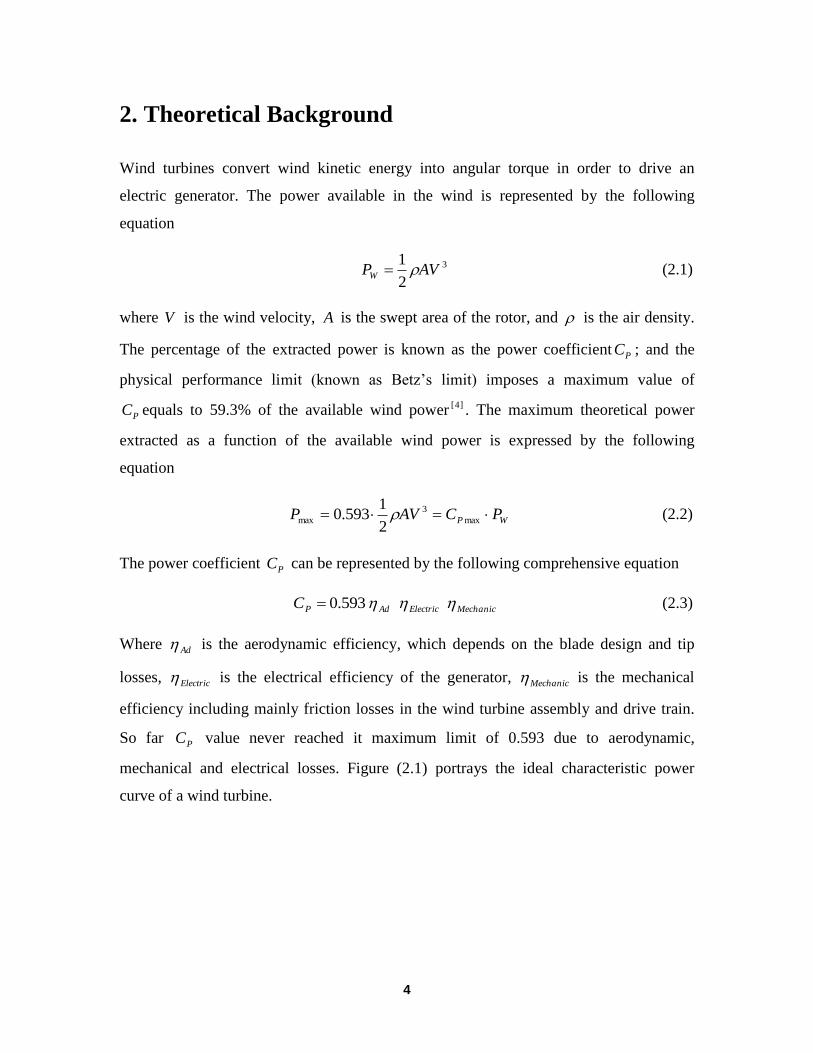
The power coefficient PC can be represented by the following comprehensive equation
593.0PC Ad Electric Mechanic (2.3)
Where Ad is the aerodynamic efficiency, which depends on the blade design and tip
losses, Electric is the electrical efficiency of the generator, Mechanic is the mechanical
efficiency including mainly friction losses in the wind turbine assembly and drive train.
So far PC value never reached it maximum limit of 0.593 due to aerodynamic,
mechanical and electrical losses. Figure (2.1) portrays the ideal characteristic power
curve of a wind turbine.

5
Figure 2.1: Ideal wind turbine power curve [1]
A very important characteristic design value is the tip speed ratio , which is a
dimensionless variable described by the following equation
V
R (2.4)
where R is the rotor radius, measured from rotor center to blade tip, and is the rotor
rotational speed.
The optimum tip speed ratio for 3-bladed grid-connected wind turbines is around =7 ]2[ ,
which means that the blade tip tangential velocity is 7 times the free wind velocity.
Moreover, operating at the optimum tip speed ratio means that we are extracting as much
power as possible from the wind.
One of the first experimental procedures for the characterization of wind turbines is
plotting the turbine’s power coefficient ( PC ) against tip speed ratio ( ). Figure (2.2)
illustrates typical ( PC - ) curves at various pitch angles.

6
Figure 2.2: Typical (Cp - λ) curves at various pitch angles [3]
Figure 2.3 shows the different angles, velocities and aerodynamic forces on a blade
airfoil.
Figure 2.3: Velocities and aerodynamic forces on a blade airfoil [3]

7
The pitch angle (also called the blade angle) is defined as the angle between the airfoil
chord and the rotor plane of rotation, measured at the blade root. Changing the pitch
angle will change the angle of attack , according to the following equation
(2.5)
r
V
1tan (2.6)
where is the angle between the rotor plane and the local wind (also called relative wind
or apparent wind or resultant wind), is the angle between the local wind and the airfoil
chord, V is the free wind velocity, is the rotational speed, r is the radius at the point of
computation measured from the rotor center. The local wind velocity vector varies along
the blade’s span according to the following equation
22 rVVres (2.7)
Figure 2.4 illustrates the aerodynamic forces acting on a blade element, the resultant of
all pressure and friction forces can be characterized by two forces and a moment (lift,
drag and pitching moment), which are all translated and calculated at the aerodynamic
center (one fourth of the chord length).
Figure 2.4: Aerodynamic forces on a blade segment [4]
An important non-dimensional parameter for defining the characteristics of fluid flow
conditions is the Reynolds number (Re) which is defined by
8
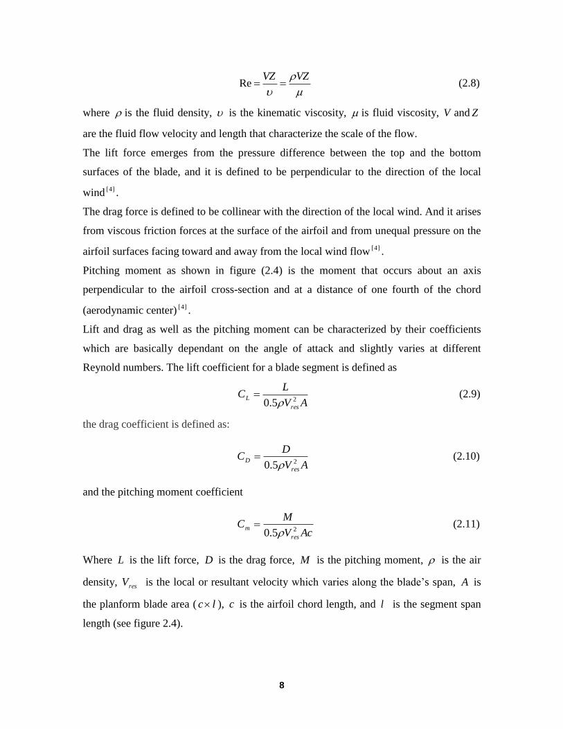
VZVZRe (2.8)
where is the fluid density, is the kinematic viscosity, is fluid viscosity, V and Z
are the fluid flow velocity and length that characterize the scale of the flow.
The lift force emerges from the pressure difference between the top and the bottom
surfaces of the blade, and it is defined to be perpendicular to the direction of the local
wind ]4[ .
The drag force is defined to be collinear with the direction of the local wind. And it arises
from viscous friction forces at the surface of the airfoil and from unequal pressure on the
airfoil surfaces facing toward and away from the local wind flow ]4[ .
Pitching moment as shown in figure (2.4) is the moment that occurs about an axis
perpendicular to the airfoil cross-section and at a distance of one fourth of the chord
(aerodynamic center) ]4[ .
Lift and drag as well as the pitching moment can be characterized by their coefficients
which are basically dependant on the angle of attack and slightly varies at different
Reynold numbers. The lift coefficient for a blade segment is defined as
AV
LC
res
L 25.0 (2.9)
the drag coefficient is defined as:
AV
DC
res
D 25.0 (2.10)
and the pitching moment coefficient
AcV
MC
res
m 25.0 (2.11)
Where L is the lift force, D is the drag force, M is the pitching moment, is the air
density, resV is the local or resultant velocity which varies along the blade’s span, A is
the planform blade area ( lc ), c is the airfoil chord length, and l is the segment span
length (see figure 2.4).

9
Figure 2.5 depicts the variation of lift and drag coefficients with the angle of attack.
Figure 2.5: LC and
DC vs. angle of attack [5]
As shown in figure 2.5, when the angle of attack exceeds 14°, the stall phenomenon takes
place, which can be physically defined as the separation of flow that leads to dramatic
drop in lift force and rise in drag force. The lift to drag ratio is an important design factor,
on which the aerodynamic performance is based ]4[ . Changing the optimum angle of
attack (13°-14° in figure 2.5) will directly lower the maximum lift to drag ratio, and this
will end up reducing the maximum aerodynamic input torque, hence reducing the power
output.
There are two strategies to limit the power output at high wind speeds, either by
increasing the angle of attack via what’s called active stall control (or pitch to stall), or by
decreasing the angle of attack, to avoid the stall, through feathering the blades (pitch to
feather).
Accordingly, pitch control is used to limit the power output of wind turbines, in order not
to exceed the rated output power, which might lead to the failure and damage of the
generator. Figure (2.6) illustrates the pitch to feather control strategy for a variable-speed
variable-pitch wind turbine.

10
Figure 2.6 Basic variable-speed variable-pitch (pitch-to-feather) control strategy [6]
The strategy shown in figure 2.6 varies depending on the wind speed. At low wind
speeds N
VV (where N
V is the wind speed correspondent to the generator rated
rotational speed N on the maxPC locus), the locus of the maximum power coefficient is
tracked, in order to extract the maximum possible energy. As the wind speed increases,
the rotational speed increases proportionally (assuming a constant tip speed ratio ).
Point B represents the point at which the blade feathering gradually starts to take place in
order not to exceed the generator’s rated rotational speed N . As seen in figure 2.6,
point C is not located on the maxPC locus, which means that at that point, less wind
energy is extracted and the wind turbine is operating at it s rated power NP .
11
3. Wind Turbine Model
In this chapter, the specifications and main components as well as the pitching system of
the wind turbine model are discussed in details.
3.1 Specifications and main components
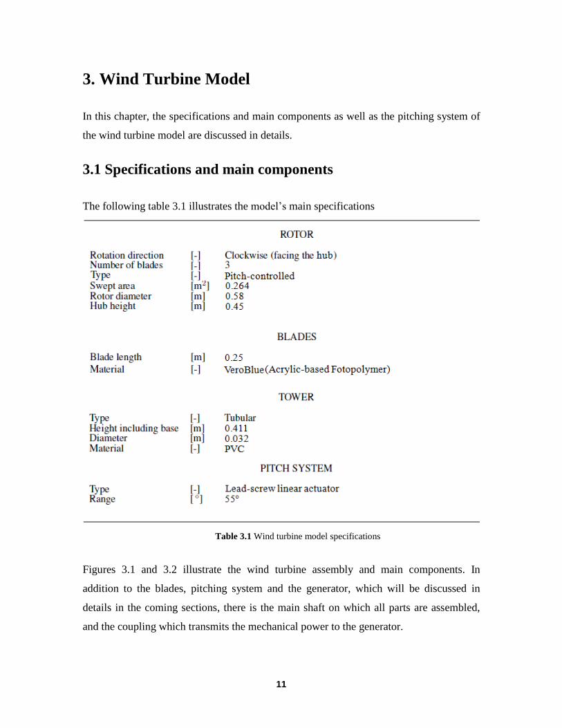
The following table 3.1 illustrates the model’s main specifications
Table 3.1 Wind turbine model specifications
Figures 3.1 and 3.2 illustrate the wind turbine assembly and main components. In
addition to the blades, pitching system and the generator, which will be discussed in
details in the coming sections, there is the main shaft on which all parts are assembled,
and the coupling which transmits the mechanical power to the generator.

12
Figure 3.1 Wind turbine main components
Figure 3.2 Nacelle assembly
As shown in figure 3.2, the nacelle consists of 5 segments (made of PVC), which are
connected using two long screw nuts.
13
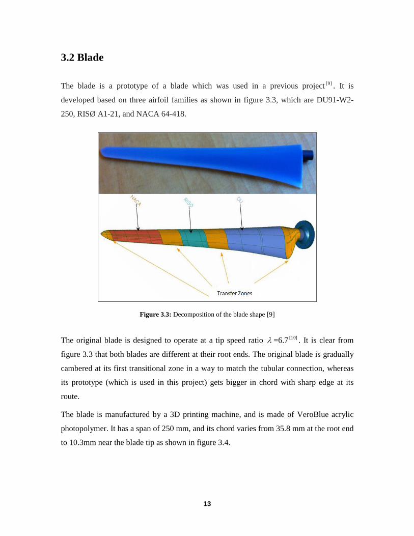
3.2 Blade
The blade is a prototype of a blade which was used in a previous project ]9[ . It is
developed based on three airfoil families as shown in figure 3.3, which are DU91-W2-
250, RISØ A1-21, and NACA 64-418.
Figure 3.3: Decomposition of the blade shape [9]
The original blade is designed to operate at a tip speed ratio =6.7 ]10[ . It is clear from
figure 3.3 that both blades are different at their root ends. The original blade is gradually
cambered at its first transitional zone in a way to match the tubular connection, whereas
its prototype (which is used in this project) gets bigger in chord with sharp edge at its
route.
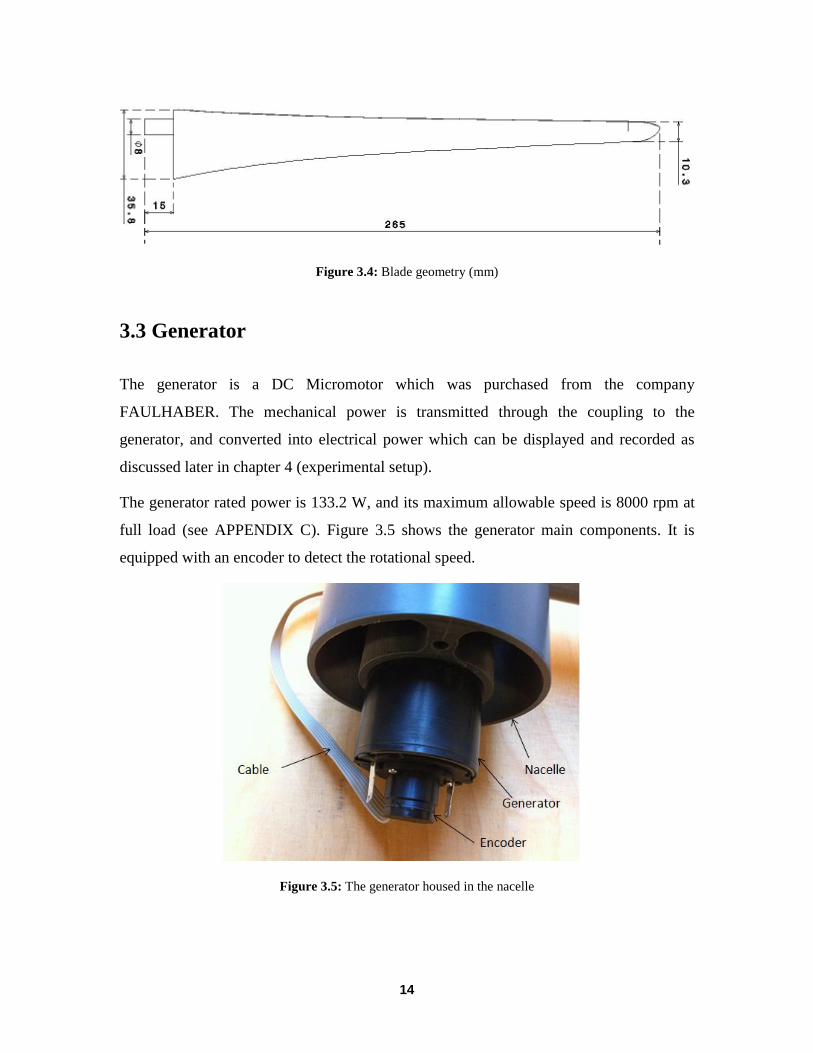
The blade is manufactured by a 3D printing machine, and is made of VeroBlue acrylic
photopolymer. It has a span of 250 mm, and its chord varies from 35.8 mm at the root end
to 10.3mm near the blade tip as shown in figure 3.4.
14
Figure 3.4: Blade geometry (mm)
3.3 Generator
The generator is a DC Micromotor which was purchased from the company
FAULHABER. The mechanical power is transmitted through the coupling to the
generator, and converted into electrical power which can be displayed and recorded as
discussed later in chapter 4 (experimental setup).
The generator rated power is 133.2 W, and its maximum allowable speed is 8000 rpm at
full load (see APPENDIX C). Figure 3.5 shows the generator main components. It is
equipped with an encoder to detect the rotational speed.
Figure 3.5: The generator housed in the nacelle

15
The selection criterion was based on a rated wind speed of 12 m/s and a power coefficient
of 0.4 using equation (1.2) as follows:
WWCAVCPP PPW 2.13357.1094.01229.02.12
1
2
1 32
max
3
maxmax
3.4 Stepper Motor
The stepper motor is used to control the pitch angle using a leadscrew mechanism. The
motor’s holding torque is 22 mNm (see APPENDIX C).
A special driver AD CM M1S is used (see APPENDIX C). AD CM M1S is a current
mode driver, the current level can be controlled by on-board switches, which allows to
apply a much higher voltage than needed to drive the current without risk of overheat.
Additionally, it can increase torque output of the motor plus give the possibility to boost
the current if necessary. The command side of the driver is connected to NI USB-6211
Analog-Digital converter ]11[ , which sends and receives digital signals to and from the
computer. Figure 3.6 shows the stepper motor wiring.
Figure 3.6: Stepper motor wiring

16
LabVIEW software is used to generate pulse trains and control the motion of the stepper
motor including number of input steps and sense of rotation CW/CCW. On the other,
LabVIEW can display the results detected from the encoder, such as the angular position.
For further information about the program please refer to APPENDIX B.
3.5 Pitching System
3.5.1 Pitching Mechanism
The pitching system is shown in figure 3.7. It consists of L-shaped slider made of Teflon
(with low coefficient of friction of 0.04), and is bored on both its upper and lower parts.
The main shaft is fitted with a tube which is made of Teflon as well. A small tolerance
was kept in order to allow the rotation of the main shaft through the lower hole of the
slider. The screw nut is fitted in the upper hole of the slider.
Figure 3.7: Pitching system components
The lead screw translates the rotational motion into linear motion as shown in figure 3.8.
Figure 3.8: Principle of operation of the traveling-nut linear actuator

17
By moving the slider back and forth (depending on the motor’s sense of rotation), the
base moves and three connected branches move accordingly (one branch consists of two
connected links), which will end up changing the pitch angle as shown in figure 3.9.
Figure 3.9: Changing the pitch angle manually
3.5.2 Load Analysis
The main criterion which was followed for the selection of the stepper motor is
calculating the pitching moment at a maximum wind speed of 15 m/s and optimum tip
speed ratio of =6.7 (referring to the original blade ]10[ ).
sradR
V/347
29.0
157.6
Referring to equation (2.11), the pitching moment at the aerodynamic center ( c /4)
measured from the leading edge equals to
cAVCM resm
25.0
Where mC is the pitching moment coefficient,
= 1.225kg/m3, resV is the local wind
velocity,
c is the chord length,
A is the planform area of the blade.
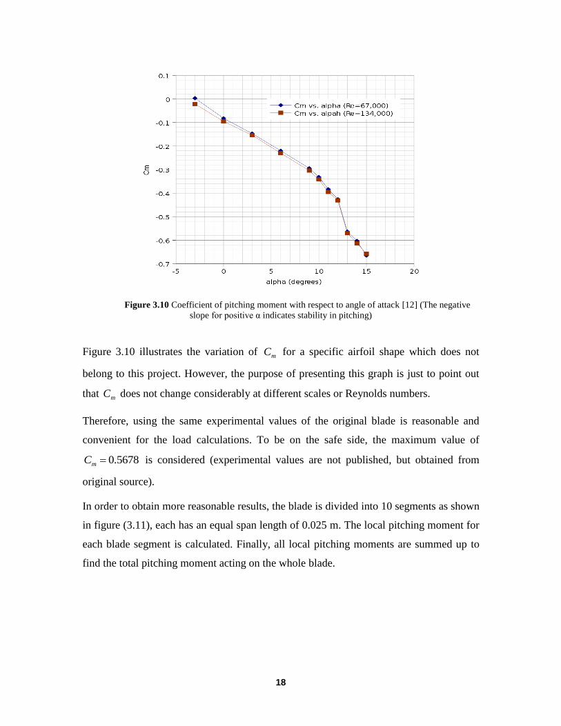
mC value depends basically on the angle of attack and varies slightly at different
Reynolds numbers as shown in figure (3.10)
18
Figure 3.10 Coefficient of pitching moment with respect to angle of attack [12] (The negative
slope for positive α indicates stability in pitching)
Figure 3.10 illustrates the variation of mC for a specific airfoil shape which does not
belong to this project. However, the purpose of presenting this graph is just to point out
that mC does not change considerably at different scales or Reynolds numbers.
Therefore, using the same experimental values of the original blade is reasonable and
convenient for the load calculations. To be on the safe side, the maximum value of
5678.0mC is considered (experimental values are not published, but obtained from
original source).
In order to obtain more reasonable results, the blade is divided into 10 segments as shown
in figure (3.11), each has an equal span length of 0.025 m. The local pitching moment for
each blade segment is calculated. Finally, all local pitching moments are summed up to
find the total pitching moment acting on the whole blade.

19
Figure 3.11: Local velocity vector at various blade segments
Following is a sample calculation for segment “1”
nn
n
resnm
n
n cAVCMM
10
1
2
)(
10
1 2
1 (3.1)
11
2
112
1cAVCM resm (3.2)
21
22
1 rVV res (3.3)
Assuming a linear variation of the chord length along the blade’s span, the mean chord
for each segment can be calculated following the formula
ncn10
103.0358.00358.0
(3.4)
mc 03325.01
24
1 1031.803325.0025.0 mA (Blade segment planform area)
22222
1 /9.5560525.034715 smV res
mNM .1035.5 3
1
The total pitching moment for one blade equals to 31013.113 M Nm.

20
Figure 3.12 shows the initial position and the dimensions of one branch in the pitching
system. The initial position of the branch is the position which corresponds to the initial
blade angle (before any pitching takes place).
Figure 3.12 Branch dimensions (Initial position)
In order to find the load acting on the lead screw, the forces acting on one branch are
calculated, by simply performing a static force analysis as shown in figure 3.13
Figure 3.13 Member force analysis

21
Defining member BC as member 1, member AB as member 2, and the lead screw as
member 3, the force applied from member 3 to member 2 (which is the lead screw force
32F ) is calculated as follows
Sum of moments at point C equals to zero (Member 1)
NM
FM C 07.708.44sin1023
0321
(Values taken from figure 3.12) (3.5)
1221 FF (3.6)
Sum of forces in the “y” direction equals to zero (Member 2)
NFFFFy 07.70 323212 (3.7)
Total force acting on all branches = lead screw force = NF 2.213 32
Figure 3.14 Screw geometry and force analysis
The Torque needed to overcome the calculated lead screw force is found using the
following power screw formulas:
ab
abFdTorque
tansec1
tansec
2
2
(3.8)
2
tand
Pitcha
(3.9)

22
Where a is the lead angle, b is half the thread angle which equals to 30°, is the
coefficient of friction between the screw and the nut which are made of brass and bronze
respectively (it is considered =0.2 for safety), Pitch equals to 0.5 mm, 2d is the
nominal diameter (For M6 screw 2d = 6 mm).
0265.0106
105.0tan
3
3
a
mNTorque .1009.13 3
Additionally, the friction due to part of the weight acting on the screw nut can be roughly
estimated. For safety considerations, the weight of the highlighted part (red dashed) in
figure 3.15 is considered (which is more than the actual acting force since the two ball
bearings fixed on the Nacelle stand part of the main shaft’s weight).
Figure 3.15 Friction force acting on the lead screw
The total weight including the blades and the hub was measured on a digital scale and
equals to 1.57N. Calculating for the frictional force
NNF 314.057.12.0 (3.10)
This can be added to the total lead screw load, the recalculated torque including frictional
forces equals to 13.28 mNm. As mentioned in section 3.4, the holding torque of the
stepper motor equals to 22 mNm. Accordingly, the factor of safety can be calculated as
follows

23
66.11028.13
10223
3
max
T
Tf critical
safety (3.11)
3.4.3 Pitch Angle Calculation
The main goal is to detect and control the pitch angle position, and for that purpose it is
required to know exactly the number of steps done by the stepper motor. The stepper
motor is designed to move 24 steps per revolution, with a 15° change in shaft’s angle per
step, and each step consists of 5 pulses (3° per pulse).
Since the step ( S ) is the smallest unit that can be entered as a variable for the motion
control, and the shaft angle is the only variable that can be detected from the stepper
motor encoder, the screw linear distance ( X ) as a function of the shaft angle in
degrees can be expressed as follows
360
5.0
360
)(screwPitchX (3.12)
S15 (3.13)
It is important to mention that M6 standard screw has a pitch of 1 mm, whereas the screw
which is used in this pitching system is specially designed and manufactured to have 0.5
mm. The reason for that is to have less pitch angle difference corresponding to the linear
motion, and therefore higher precision in controlling the pitch angle.
Now that the linear motion is detected, it is still required to find the pitch angle as a
function of the linear motion.
Considering one branch as shown in figure (3.16)

24
Figure 3.16 Animation of linear and angular motion
The system can be mathematically presented as follows
cos23cos25 dX (3.14)
16sin25sin23 (3.15)
From the initial position ( X =0):
52.4108.44cos230cos25 d
the equation can be rephrased as:
cos23cos2552.41 X (3.16)
From equation 3.15
25
16sin23sin 1
(3.17)
Substituting in equation 3.14
25
cos2325
16sin23sincos25523.41 1
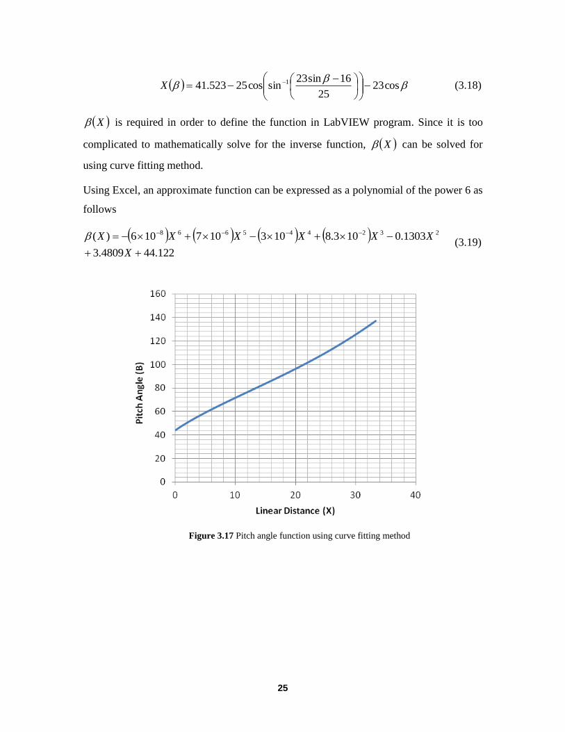
X (3.18)
X is required in order to define the function in LabVIEW program. Since it is too
complicated to mathematically solve for the inverse function, X can be solved for
using curve fitting method.
Using Excel, an approximate function can be expressed as a polynomial of the power 6 as
follows
122.444809.3
1303.0103.8103107106)( 232445668
X
XXXXXX (3.19)
Figure 3.17 Pitch angle function using curve fitting method

26
4. Wind Tunnel Testing
The purpose of this project is to design and characterize a small wind turbine model. Now
that the design issues and considerations are discussed in details, the experimental set up
and the characteristic curves of the wind turbine are summarized in this chapter.
4.1 Experimental Setup
Figure 4.1 portrays the system setup
Figure 4.1 Circuit Diagram
The circuit diagram illustrates the connections and the information flow in the system,
basically the inputs and the outputs of the stepper motor and the generator. From the
generator, it is required to detect the rotational speed, voltage and current values which

27
are necessary for the characterization of the wind turbine (( PC - λ) curves).
Simultaneously, a voltmeter and an ammeter are used, in order to check that the readings
displayed on LabVIEW program comply with the measured values. The electric output
power is simply calculated by the multiplication of both variables P=VI. For further
details regarding the electrical control circuit which was used for the load
characterization, please refer to ]13[ .
For the stepper motor, it is required to track the pitch angle position following the
correlations explained in section 3.4.3. This happens by sending and receiving digital
signals using LabVIEW pitch control program as shown in the circuit diagram.
The wind turbine model is fixed facing the incoming wind as shown in figure (4.2). The
wind speed can be controlled using the control panel over the range (1 m/s - 50 m/s), but
for safety considerations concerning the blade durability, a maximum wind speed of 14
m/s was considered in this project.
Figure 4.2 The wind turbine positioned within the wind tunnel

28
Additionally, two computers were used for the characterization process, one for
controlling the stepper motor (pitch angle control) and the other for detecting the
rotational speed and the power output of the generator.
Before starting the test run, the initial pitch angle 20 is set (measured at the blade
root) as shown in figure 4.3. The figure represents the smallest pitch angle which can be
reached in the system (angle between the chord the rotor plane).
Figure 4.3 Setting of the initial pitch angle
4.2 Test Procedure and Data Recording
After setting up the system, the experiment started by operating the wind tunnel at low
wind speeds to find out the cut-in speed. The cut-in speed was 3.5 m/s. However,
experimental measurements were first conducted at wind speed 4 m/s to avoid high
fluctuation in frequency readings.
At each wind speed, the pitch angle is changed (starting at 20°) with a steady increment
of 1°. At each pitch angle setting, the rotational speed is changed by changing the load
from 5 Ω to 50 Ω with a steady increment of 5 Ω. At each load setting the power output is
measured, and finally the ( PC - λ) curves are plotted. For further details regarding the
load characterization, please refer to ]13[ .

29
It was found out after repeating the previous procedure over the wind speed range 4 m/s–
9 m/s, that the optimum pitch angle is 21° for all wind speeds.
4.3 Characteristic Curves
Figure (4.4) illustrates the ( PC - λ) curves at different pitch angles at wind speed 9 m/s
Figure 4.4 (Cp- λ) curve at various pitch angles at wind speed 9 m/s
As shown in figure 4.4, the maximum PC occurred at pitch angle 21 ( PC (max) =0.022,
maximum power output = 2.52 Watt). The optimum tip speed ratio was =3.21. The
maximum power output values at wind speeds up to 9 m/s were used to plot the first part
of the characteristic power curve as shown in figure (4.5).
Figure 4.5 depicts the wind turbine power characteristic curve. It is important to mention
that the wind speed 9 m/s is considered as the “presumed” rated wind speed. Therefore,
the power characteristic curve does not represent the actual system’s limitations, but the

30
assumed limitations. A comprehensive accurate characterization of the wind turbine
model can be recommended for future work.
Figure 4.5 Wind turbine model power curve
31
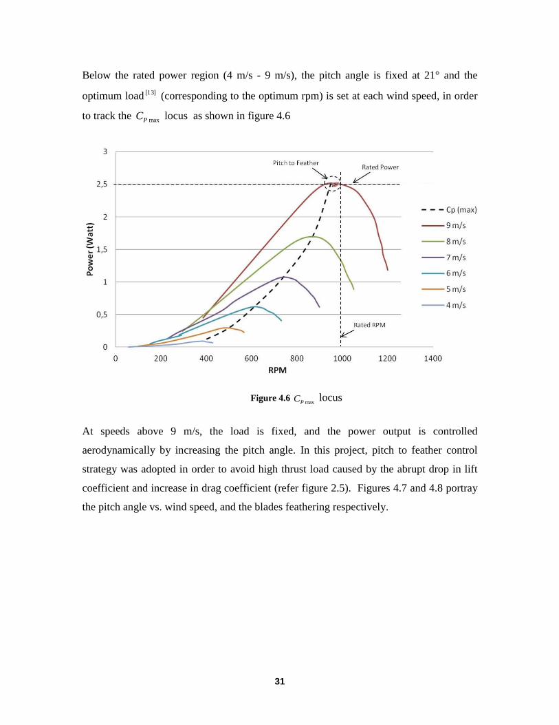
Below the rated power region (4 m/s - 9 m/s), the pitch angle is fixed at 21° and the
optimum load ]13[ (corresponding to the optimum rpm) is set at each wind speed, in order
to track the maxPC locus as shown in figure 4.6
Figure 4.6 maxPC locus
At speeds above 9 m/s, the load is fixed, and the power output is controlled
aerodynamically by increasing the pitch angle. In this project, pitch to feather control
strategy was adopted in order to avoid high thrust load caused by the abrupt drop in lift
coefficient and increase in drag coefficient (refer figure 2.5). Figures 4.7 and 4.8 portray
the pitch angle vs. wind speed, and the blades feathering respectively.

32
Figure 4.7 Pitch angle vs. wind speed
Figure 4.8 Feathering the blade

33
5. Results and discussion
In this chapter, the results of the characterization procedure are discussed and analyzed.
Additionally, some future improvements and recommendations are suggested for future
work.
5.1 Data Analysis
Table 5.1 illustrates the characteristic data at the rated wind speed 9 m/s and pitch angle
21°.
Resistor (Ω)
Speed (rpm)
Generator Voltage (V)
Current (A)
Power (W)
2,5 385,864913 1,062794 0,423534 0,450129
5 766,856792 3,323003 0,599413 1,991853
7,5 875,984028 4,260041 0,561916 2,393787
10 950,149703 5,045075 0,499275 2,518879
15 1049,201308 6,06156 0,399721 2,422934
20 1104,1374 6,692095 0,328361 2,197424
25 1141,521722 7,099527 0,276176 1,960722
30 1157,757428 7,377506 0,234855 1,732642
35 1173,512015 7,556504 0,205143 1,550167
40 1178,649985 7,732923 0,183177 1,416494
45 1192,148557 7,82656 0,163356 1,278518
50 1199,159242 7,944152 0,149032 1,183931
Table 5.1 Characteristic data at rated wind speed 9 m/s and pitch angle 21°
As shown in the table, the maximum power output takes place at a resistance of 10 Ω
(corresponding speed of 950 rpm). The wind power available at wind speed 9 m/s can be
calculated using equation 1.1 as follows
WattPW 56.1159*29.0**2.1*2
1 32
022.056.115
52.2pC

34
21.3960
29.015.9502
60
2
V
nR
V
R
Table 5.2 shows the characteristic details for the power controlled region (9 m/s – 14 m/s)
Table 5.2 Characteristic details for the power controlled region
Figure 5.1 illustrates the PC values at all wind speeds. maxPC varies in both below and
above rated wind speed (9 m/s). At wind speeds above 9 m/s, maxPC decreases due to
pitch control and this is desired to maintain constant power.
At lower speeds such as 4 and 5 m/s, there is very little wind energy available and most
of it is needed to overcome frictional and electrical losses in the wind turbine ]14[ .

35
Figure 5.1 maxPC vs. Wind speed
Figure 5.2 illustrates the variation of optimum tip speed ratio under different wind speeds.
Figure 5.2 λ vs. Wind speed

36
As shown in the previous tables and figures, the values of PC are too low, and does
not reach half of the expected value ( =6.7 for the original blade of MEXICO
project ]10[ ). Following are some possible reasons for the unexpected results
1. The discrepancy in the initial blade angle setting between the three blades affects
the aerodynamic efficiency. The initial pitch angle (20°) is not exactly the same
for all three blades, which means that each blade operates at a different angle of
attack, and therefore different lift and drag coefficients. The reason of this
discrepancy is that no precision measurement tool was used to set exactly the
same angle for all blades and it was measured with the naked eye.
As an example for the blade’s angle discrepancy effect, the following figure 5.3
depicts the difference in power coefficient and tip speed ratio for two different
setups. In the first setup, there was one blade which had about 10° discrepancy
(measured with the naked eye) compared to the other two blades. In the second
setup (which was the setup adopted for the characterization), the three blades were
set at nearly the same angle (20°).
Figure 5.3 (Cp - λ) curves at first and second setup

37
The figure depicts the sensitivity to discrepancies and the necessity to use a
precision measurement tool to ensure exactly the same pitch angle for all blades.
2. Any inaccuracy in the blade manufacturing or any discrepancies in the blade’s
curvature, twist angle or chord length will affect the aerodynamic efficiency of the
wind turbine.
3. The inaccurate scaling of MEXICO wind turbine model (which will be handled
thoroughly in section 5.2).
4. The system has high friction and electrical losses, and this can be observed clearly
at lower wind speeds.
5. The components along the main shaft might be misaligned with each other, and
one of the possible reasons is the absence of a fixation point or bearing close to
the hub (see figure 3.15). The front part of the main shaft could be fixed to the
nacelle to ensure a better alignment.
6. Further design considerations for the stability of the tower structure are desired,
since high vibration of the machine at high wind speeds was observed.
7. There might be high electrical losses (wasted power) due to using a variable
resistor for the speed control ]15[ .

38
5.2 Improvement
As mentioned in the previous section, the highest optimum tip speed ratio as shown in
figure 5.2 is about half the optimum tip speed ratio of MEXICO project blade ]14[ .
One of the reasons for this considerable difference can be the wrong model scaling.
Wrong scaling means that for the same pitch angle and at a specific point of computation,
there are different chord lengths and twist angles. As a result, there are different
aerodynamic forces and coefficients (lift and drag) compared to the original model.
Figure 5.4 shows the original blade’s span length and distances measured from rotor
center.
Figure 5.4 original blade’s dimensions (mm)
The dashed extension represents the design difference between the MEXICO project
blade and its prototype, while the rest remains the same for both blades (see also figure
3.3).
The comparison starts at the distance 91DUr , which is the distance from the rotor center to
the first section of the airfoil family DU91 as illustrated in the decomposition of the blade
(figure 3.3). The point of computation 91DUr was selected since it is the first common
section to both blades. Figure 5.5 illustrates the offset in both the chord length and the
twist angle due to the wrong scaling.

39
Figure 5.5 Twist angle and chord length offset (experimental values are not published, but
obtained from original source)
The figure reveals an offset of 2° in twist angle and about 7% deviation in the scaled
chord length at the point of computation 91DUr , which means that both blades are facing
different aerodynamic conditions.
Compared to the prototype blade (figure 3.11), the ratios of the distances between the
rotor center to blade root ( rootr ) over the rotor center to the blade tip ( R ) in both blades
differ considerably as follow

40
102.02250
230
R
rroot (MEXICO model)
138.0290
40
R
rroot (Our model)
And since the chord length and the twist angle are functions of the radius at the point of
computation (measured from the rotor center), the same function for both blades should
be maintained using the correct scaling in order to maintain similar aerodynamic
conditions. And this can be done by either decreasing the rotor center to blade root
distance ( rootr ) by reducing the hub size, or by increasing the dimensions of the blade to
match the same twist angle and chord length functions along the blade’s span.
As the internal space of the hub is already used to house the pitching mechanism, a
recommendation could be to increase the blade size proportional to the original blade.
The new distance from the rotor center to the blade tip can be calculated as follows:
mmr
R root 391102.0
40
102.0
New blade length equals to
mm35140391
75.5351
2020Scale
(Scale 5.75:1)
All other dimensions including the chord lengths and blade twisting should follow the
same scale. Figure 5.6 shows the recommended blade’s dimensions.
Figure 5.6 recommended model blade’s dimensions (mm)

41
5.3 Recommendations
Following are some future recommendations
1. Using a precision measurement tool to accurately set the initial blade angle
2. Setting of the initial blade angle below 20° (preferably at 0°), in order to apply
pitch to stall control method.
3. Ensure good lubrication for the bearings
4. Ensure a better alignment of the main shaft components by adding an extra
bearing close to the hub and fix it to the nacelle, or by adding a roller support as
shown in figure 5.7. This will also transfer the extra load on the screw nut to the
nacelle body (see figure 3.15).
Figure 5.7 Roller support
5. Further design considerations for the stability of the tower structure are
recommended in order to eliminate vibrations as mentioned in section 5.1.
6. Using a more efficient method to control the rotational speed rather than a
variable resistor or a rheostat.

42
6. Conclusion
Small wind turbines can be very sensitive to small design mistakes or discrepancies in
prototyping. Consequently, special attention to details and precise design issues should be
taken into consideration when it comes to characterization of small wind turbines.
Linear actuators or lead screws are convenient for pitch control systems, since they need
small torque to overcome high pitching moment, which makes it more feasible and
attractive compared to other automatic pitch control systems.
Pitch to feather control is a convenient way to limit the wind turbine power output, since
the high thrust load can be avoided. The disadvantage of pitch to feather technique is the
need of the continuous and intensive pitch angle control in order to assure a constant
power output.

43
References
1. http://www.wind-power-program.com/turbine_characteristics.htm
2. Optimal Rotor Tip Speed Ratio, ©M. Ragheb, 4/15/2011
3. Wind turbine control algorithms. Technical Report ECN-C--03-111, E.L. van der
Hooft; P. Schaak; T.G. van Engelen, December 2003.
4. Wind Energy Explained: Theory, Design and Application. James F. Manwell, Jon G.
McGowan, Anthony L. Rogers, 2009
5. http://www.ecn.nl/nl/nieuws/newsletter-en/2010/june-2010/turbine-blades-less-fatique/
6. Fernando D. Bianchi, Hernán De Battista and Ricardo J. Mantz, April 2006, Wind
Turbine Control Systems Principles, Modelling and Gain Scheduling Design
7. Aufbau und Inbetriebnahme einer Messeinrichtung für Modelluntersuchungen an
Rotorblättern von Windkraftanlagen, Daniel Schütze, Berlin, 2008
8. Konstruktion und Aufbau einer Messeinrichtung für Modelluntersuchungen an WEA-
Rotoren mit dem Hochlaufversuch, Staffan Wallmann, David Janke, Berlin, 2008
9. http://www.ecn.nl/nl/nieuws/newsletter-en/2009/december-2009/aerodynamics-wind-
turbines/
10. The MEXICO project (Model Experiments in Controlled Conditions): The database
and first results of data processing and interpretation, H Snel, J G Schepers and B
Montgomerie, 2007
11. http://sine.ni.com/nips/cds/print/p/lang/en/nid/203224
12. Clancy, L.J. (1975), Aerodynamics, Pitman Publishing Limited, London
13. Design and Power Characterization of a Small Wind Turbine Model in Partial Load
Region, Abdulkarim Abdulrazek, Oldenburg, 2012
14. http://www.mpoweruk.com/wind_power.htm
15. http://www.peoi.org/Courses/Coursesen/circuit2/ch/ch9e.html

44
APPENDIX A

45
APPENDIX B

46

47
APPENDIX C

48

49

50

51

52

53

54

55

56

57

58