Embed Size (px)
Citation preview
Design and analysis of a semi-submersible vertical axis wind turbine
Muhammad Abu ZafarSiddique
Marine Technology
Supervisor: Zhen Gao, IMT
Department of Marine Technology
Submission date: June 2017
Norwegian University of Science and Technology


i
Preface
This thesis is submitted to the Norwegian University of Science and Technology (NTNU) for
partial requirements to fulfill M.Sc. program.
This thesis is carried out the at the at the Department of Marine Technology under the supervision
of Professor Zhen Gao at the department of Marine Technology, NTNU and the Co-supervisor
Zhengshun Cheng. I am indebted to them. They helped me a lot and guide me to the proper
direction. Also, I would like to thank Associate professor Erin Bachynski, Department of Marine
Technology and PhD candidate Yuna Zhao who helped me to learn SIMA software. I would like
to thank my colleague. They helped me a lot during my thesis.
The thesis was carried out from January 2017 to June 2017.
ii
Abstract
Wind energy are deployed by two types of wind turbines. They are Horizontal Axis Wind Turbine
(HAWT) and Vertical Axis Wind Turbine (VAWT), classified according to their axis of rotation.
In recent years, offshore wind energy playing a vital role in the wind turbine industry due to high
intensity of air, less turbulent and comparatively clean and easily employed in large area which is
difficult to manage for onshore or near-shore. The advantages of HAWTs are now facing different
challenge in the offshore field due to its cost effectiveness . For this reason, VAWTs have the
potential to reduce the cost of producing per unit power. Hence, the emergence and growing
interest for VAWTs for offshore application.
The availability of fully coupled simulation tools are extremely limited and more sophisticated
tools are necessary to carry out the simulation in a fully coupled manner. In this thesis, we used
SIMO-RIFLEX-AC for the fully coupled simulation developed by NTNU/MARINTEK. SIMO is
capable to calculate the rigid body hydrodynamics forces and different moments on the floater
which is designed to support the VAWT. RIFLEX is used to model the tower, blades, struts,
mooring lines as flexible finite elements. To calculate the aerodynamic loads acting on the wind
turbine we used Actuator Cylinder (AC) model. In addition, it accounts the effect of wind shear
and turbulence, dynamic stall by using BL (Beddoes-Leishman) model and dynamic inflow. Then
this code was coupled with SIMO-RIFLEX to carry out the integrated analysis.
To carry out the fully coupled simulation in time domain, a model was developed in HydroD and
analyze the response in the frequency domain. The model was then modified in SIMO and used
for coupled simulation. This model is used to study the various cases such as decay test, steady
wind test and turbulent and irregular wave test. Also, we carried out a study on the second order
mean drift force to check the response of the system. To calculate the second order effect, we use
Newman approximation, otherwise to evaluate the second order transfer function is really time
consuming. Then we compare our data with different types of vertical wind turbine such as OC4
semi-submersible and landbased wind turbine and carried out a detail study. We focus our study
on motion response; performance of the wind turbine such as power, rotor speed, thrust, torque;
mooring line tension and tower base bending moment. We also carried out power spectral analysis
to see response in different frequency ranges. Considering three wind load cases such as one is
below rated speed, one is the rated speed and the last one is above rated speed. The later study was
carried out by using the WAFO which is used as a MATLAB routines.
One of the focus of the study is to optimize the original OC4 semi-submersible used to support the
NREL 5MW wind turbine. The optimization was carried out in terms of reducing the weight and
reducing the principal parameters of the platform which was carried out in the project. The
optimization was satisfactory in terms of weight and its behavior because the modified OC4 semi-
submersible preserve the main characteristics such as natural frequency and damping ratio.
In general, a fully coupled analysis was carried out to observe the dynamic characteristic of the
wind turbine and applied the results to compare its characteristics with other floating and landbased

iii
VAWTs. This will in turn helps us to reveal the advantages and disadvantages of using vertical
axis wind turbine than horizontal axis wind turbine. Also, it will help to understand dynamic
characteristics and behavior of different wind turbines.

iv
Acknowledgement
First, I would like to express my immense gratitude to my supervisor Professor Zhen Gao to work
under him. It’s been almost one year since I started my work with him. Then I started to work for
my thesis since January 2017. It’s been five month since I worked with him for my thesis. During
this period, we met once a week and discuss our work. He helped me and guide me like a true
mentor. In this thesis, I always stumbled with some difficulty and professor was always there to
help me. I was truly benefitted from his discussion, his insight on the topic.
Secondly, would like to thank my co-supervisor Zhengshun Cheng. I respect him for his patience
on me during this time due to my silly question or silly mistake. He literally taught me the very
foundation of the software that I used during my thesis. Sometimes I went to his room more than
once in a single day. I spent hours to discuss and solve the problem. Whenever I stumbled, he
helped me and show me the direction. He checked my code, correcting my error in the code. Often
I sent him mail in the weekend and to my surprise he replied within two or three hours. I truly
impressed not just as a knowledgeable person but his character and the patience I observed during
this time.
Many other people helped me a lot in my thesis. Specially I would like to thank Associate professor
Erin Bachynski for her support. Sometimes I ask her question through mail. Ph.D candidate Yuna
Zhao who helped me how to use SIMA effectively. I would like to express my gratitude to my
colleague and my friends who actively support my work.
I would like to give my special thanks to my parents who actively support me from my country
Bangladesh. Also, my special thanks to my lovely wife Shanjida Hoque Sweety who helped me
during this period immensely. I want to apologize not to give her enough time. Without them, I
may never able to reach this far.
Finally, I want to thank Almighty Allah to bestow His immense mercy throughout my life.

v
Abbreviations
AC Actuator Cylinder
BEM Blade Element Momentum theory
CALHYPSO CALcul HYdrodynamique Pour les Structures Offshore
CFD Computational Fluid Dynamics
DLL Dynamic Link Library
DMS Double Multi-Streamtube
DOF Degrees of Freedom
FHAWT Floating Horizontal Axis Wind Turbine
FVAWT Floating Vertical Axis Wind Turbines
GW Gigawatt
HAWC2 Horizontal Axis Wind turbine simulation Code 2nd generation
HAWT Horizontal Axis Wind Turbine
INFLOW INdustrialization setup of a FLoating Offshore Wind turbine
ISO International Organization for Standardization
JONSWAP Joint North Sea Wave Project
LC Load Case
MW Megawatt
NACA National Advisory Committee for Aeronautics
NREL National Renewable Energy laboratory
OC4 Offshore Code Comparison Collaboration Continuation
OWENS Offshore Wind ENergy Simulation
PI Proportional-Integral
QTF Quadratic Transfer Function
RAO Response Amplitude Operator
RANS Reynolds-Averaged Navier Stroke

vi
TLP Tension Leg Platform
USSR Union of Soviet Republics
VAWT Vertical Axis Wind Turbine
WADAM Wave Analysis by Diffraction and Morison Theory
WAMIT Wave Analysis Massachusetts Institute of Technology
List of symbol
α Angle of attack/Spectral parameter
θ Angle
γ Peaked parameter
ε Phase angle
ρ Density of water
𝛿𝑖3 Kronecker-Delta function for (i,3) component
𝜑(𝑥, 𝑦, 𝑧, 𝑡) Potential function
𝜙𝛼𝐶 Non-circulatory indicial function
𝜙𝛼𝑙 Circulatory indicial function
𝜂𝑖 Platform motion
𝜔𝑑 Damping frequency
𝜔0 Natural frequency
ξ Damping ratio
∧ Logarithmic decrement
ζ Wave elevation
∇ Vector operator
𝐴𝑖𝑗 Added mass matrix
𝐵𝑖𝑗 Damping matrix
𝐶𝑎 Added mass coefficient
𝐶𝑑 Drag coefficient
𝐶𝑑𝑧 Drag coefficient in the heave direction
𝐶𝑖𝑗ℎ𝑦𝑑𝑟𝑜
(i, j) component of from the linear hydrostatic restoring matrix

vii
𝐶𝐿 Lift coefficient
𝐶𝑁𝑣 Normal force coefficient for vortex lift contribution
𝐶𝑝 Power coefficient
g Acceleration due to gravity
𝐻𝑠 Significant wave height
𝐾𝐺 Generator stiffness
𝐾𝑃 Proportional gain
𝐾𝐼 Integral gain
𝐾𝐷 Derivative gain
𝑀𝑖𝑗 Mass Matrix
n Normal vector
p Pressure distribution
𝑄𝑛 Normal forces acting on actuator cylinder
𝑄𝑡 Tangential forces acting on actuator cylinder
𝑇𝑛𝑖 Time period
𝑇𝑝 Peak time period
𝑇𝑗𝑘𝑖𝑐 Quadratic transfer function
𝑉0 Volume displacement of water
𝑉∞ Free stream velocity
(𝑥𝑏 , 𝑦𝑏 , 𝑧𝑏) Center of buoyancy
(𝑥𝑔, 𝑦𝑔, 𝑧𝑔) Center of gravity
viii
List of figures
1.1 Global annual installed capacity (1997-2014) and Global wind power cumulative capacity
2
1.2 Different kinds of VAWT 4
2.1 Layout of optimized OC4 semi-submersible 9
2.2 Schematic diagram of ladbased VAWT and OC4 floating VAWT 12
2.3 Coordinate system 13
2.4 Wave heading direction with respect to platform 15
2.5 Righting moment and wind heeling moment curves 17
2.6 Moment curve 21
2.7 Change of intercept angle by changing draft 21
3.1 Flow chart of different aerodynamic model 23
3.2 Actuator cylinder model 24
3.3 Flow chart of modelling of VAWT using AC method 31
3.4 Working process of fully coupled simulation tool 32
3.5 The generator control torque for a FVAWT 33
3.6 Time period for surge, heave, pitch and yaw 37
3.7 Damping ration for both platform 39
3.8 Time history of surge, heave, pitch and yaw (decay test) 39
3.9 Mean offset vs wind speed (surge, heave, pitch and yaw) 41
3.10 Mean offset and standard deviation of motions under different load cases
43
3.11 Mean and standard deviation of turbine performance (new FVAWT, old FVAWT and landbaed VAWT)
44
3.12 Tower base bending moment of wind turbine. Showing mean value and standard deviation for fore-aft and side-side bending moment
45
3.13 Mean and standard deviation of axial force on mooring line 1, 2 and 3
47
3.14(a) Mean offset of of different degrees of freedom 48
3.14(b) Mean offset of of different degrees of freedom 49
3.15 (a) Standard deviation of surge, sway 49
ix
3.15(b) Standard deviation of heave, roll, pitch and yaw 50
3.16(a) Power spectra for surge at LC 2.3 50
3.16(b) Power spectra for surge at LC 2.7 50
3.16(c) Power spectra for yaw at LC 2.3 51
3.16(d) Power spectra for yaw at LC 2.7 51
3.17 Mean value of rotor speed, generator power, thrust and torque 52
3.18 Standard deviation of turbine performance 53
3.19 Tension on mooring line 1, 2 and 3 54
3.20 Power spectra for mooring line 2 at LC 2.3, LC 2.5 and LC 2.7 55
3.21 Tower base fore-aft bending moment 56
3.22 Tower base side-side bending moment 56
3.23 Tower base fore-aft bending moment for LC 2.3, LC 2.5 and LC 2.7 57
3.24 Mean offset of surge, pitch and yaw(mean drfit) 60
3.25 Standard deviation of surge, pitch and yaw(mean drfit) 60
3.26 Power spectrum analysis for surge under LC 2.3 and LC 2.7 61
3.27 Power spectrum analysis for surge under LC 2.3 and LC 2.7 61
3.28 Performance of wind turbine (mean drift) 62
3.29 Mean value of mooring force on line 1, 2 and fore-aft, side-side bending moment acting on tower base (from up-down)(mean drift)
64
3.30 Standard deviation of mooring force on line 1, 2 and fore-aft, side-side bending moment acting on tower base (from up-down)(mean drift)
64
3.31 Power spectra for mooring line 2 (LC 2.3, LC 2.5 and LC 2.7) 65
3.32 Power spectra for tower base bending moment (LC 2.3, LC 2.5 and LC 2.7)
65

x
List of tables
2.1 Layout of optimized OC4 semi-submersible 9
2.2 Specification of mooring line 10
2.3 Principal parameter of straight bladed wind turbine 10
2.4 Principal parameter of the original semi-submersible 11
2.5 Specification of landbased VAWT 12
2.6 Hydrodynamic coefficients 17
3.1 Steady wind load cases for FVAWT 33
3.2 Load cases for turbulent wind and irregular waves 34
3.3 Natural time period 37
3.4 Damping ratio 38
3.5 Mean offset under different load cases 41
xi
Contents
Preface I
Abstract II
Acknowledgement IV
Abbreviations V
List of symbol VI
List of figures VIII
List of tables X
Contents XI
1 Introduction 1
1.1 General background 1
1.2 Vertical axis wind turbine 3
1.3 Floating VAWT 4
1.4 State of art in VAWT and HAWT modelling 5
1.4.1 Aerodynamic modelling 5
1.4.2 Couple analysis tool 6
1.5 Aim and scope of the study 7
2 Design and stability of Floating semi-submersible 8
2.1 Platform design 8
2.2 Old OC4 Platform 10
2.3 Fixed VAWT model 11
2.4 Coordinate system 12
2.5 Platform hydrodynamic properties 13
2.5.1 Hydrostatic loads 14
2.5.2 Hydrodynamics 14
2.5.3 Potential flow theory 14
2.6 Morison’s equation 16
2.7 Added mass 16
2.8 Intact Floating Stability 17
2.9 Modelling in SIMO 18

xii
2.10 Modifying parameters in SIMO 18
2.11 Equation of motion and natural periods 19
2.12 Stability of the Semi-submersible 20
3 Aerodynamic & Hydrodynamic loads on VAWT 23
3.1 Overview of Aerodynamic Models for FVAWT 23
3.2 The Actuator Cylinder Flow Model 24
3.2.1 Governing equations and method of solution 25
3.2.2 Linear Solution 27
3.2.3 Modified Linear Solution 29
3.3 Dynamic Stall model 29
3.4 Method of analysis 30
3.5 Coupled model for FVAWT 31
3.6 Control Strategy 32
3.7 Load cases and environmental conditions 33
3.7.1 Environment 34
3.7.2 Wind 35
3.7.3 Irregular waves 35
3.8 Decay test 36
3.8.1 Discussion of results (Natural period) 37
3.8.2 Damping ratio and the measurement technique 38
3.8.3 Discussion of results (Damping ratio) 39
3.9 Results and discussions for steady wind test 41
3.9.1 Global motions 41
3.9.2 Turbine performance 43
3.9.3 Bending moment 45
3.9.4 Mooring line tension 46
3.10 Turbulent wind and irregular waves (Results and discussion) 48
3.10.1 Global motion 48
3.10.2 Turbine performance 51
3.10.3 Mooring line tension 53
3.10.4 Bending moment 55
3.11 Second order effect 57

xiii
3.12 Modelling in HydroD 58
3.13 Newman approximation 58
3.14 Results and discussion on the effect of mean drift 59
3.14.1 Platform motion 59
3.14.2 Performance 61
3.14.3 Tower base bending and mooring line force 63
4 Conclusions and recommendation for future works 66
4.1 Conclusions 66
4.2 Recommendation for future work 67
References 68

1
Chapter 1
Introduction
1.1 General background
The use of wind energy is not a new technology but draws its inspiration on the rediscovery of a
long tradition of wind power technology. It’s not possible to tell where and when the first wind
harvesting procedure started but windmills are used to grinding grain and pumping water for at
least several thousand years. In sailing ships the wind is an essential source of power for even
longer. The spread of cheap coal and oil fuels and ease of energy distribution make people to forget
this technology. They could only survive in the economic niches of little importance [1]. But in
the of twentieth century people begin to realize how hazardous it can be for our environment and
for us. It emits different types of greenhouse friendly gas such as CO2, NOx and SOx. Fossil fuel
might provide a cheaper source of energy but in turn it takes more than we can fathom. Also, the
energy source is limited. So, they turn their attention into renewable energy source where people
do not need to think the extinction of certain energy source. It helps our environment clean because
no greenhouse gas emitted from it. Consequently, while energy production is based on the fossil
fuel or splitting the uranium atom is meeting with increasing resistance or any other reason that
might halt the progress, wind power is the inevitable consequence.
In modern times, the use of windmills to generate electricity can be traced to Charles Brush is the
USA and the research was undertaken by Poul la Cour in Denmark. Another notable achievement
was done Smith-Putnum. They developed a 1250 KW wind turbine with steel rotor 52 m in
diameter. But in 1945, a blade spar failed catastrophically. Some author recorded that the 100 KW
30 m diameter Balaclava wind turbine in USSR in 1931 and the Andra Enfield 100 KW 24 m
diameter pneumatic design constructed in the UK in the early 1950s. In Denmark, 200 KW 24m
diameter Gedser machine was built in 1956. In 1963, Electricite de France tested a 1.1 MW 35 m
diameter turbine in 1963 [2].
In the recent times, scientific community increases their investigation and develop new technique
to harvest energy from wind. Worldwide there are now more than two hundred thousand wind

2
turbines operating, with a capacity of 432 GW at the end of 2015. Worldwide wind power
generation capacity more than quadrupled between 2000 and 2006, doubling in every three years.
The new installed capacity is mainly driven by the continuation of boom in Germany, China and
USA which contributed to a capacity of 30.5 GW, nearly half of 63.01 GW installed in 2015.
World wind capacity has expanded rapidly to 336 GW in June 2014 and energy production was
around 4% of total worldwide electric power usage and growing rapidly. Europe accounted for
48% of the total wind power generation capacity in 2009. In 2010, Spain took the leading position
in Europe and produces a total of 42,796 GWh. German held the top spot in Europe and their
capacity was 27,215 MW as of 31 December 2010 [3]. The global wind power energy is increasing
on a rapid scale by constructing megawatt scale wind turbine on land or at sea. Although the power
industry is affected by the global economic crisis but GWEC predicts that the capacity of wind
power will be 792.1 GW by the end of 2020.The figure shows the cumulative capacity of global
wind power 1996-2015 and global annual installed capacity from 1997-2014.
a b
Figure 1.1: (a)Global annual installed capacity (1997-2014) (b) Global wind power cumulative capacity
Most of the wind farm are onshore based wind farm due to its cost effectiveness and maturity
comparing to the offshore wind farm. Up to this date offshore wind energy covers only a small
portion of the wind energy. By the end of 2015, it reaches 12.11 GW by the end of 2015 [4]. But
the power production increases day by day and it’s a major player in the wind sector.
In general, current offshore wind turbines are mounted on the fixed structures such as monopile,
jacket based structure or gravity platform. As the water depth increases, the only option left is
floating structure. In some countries, such as Norway, China, Japan and USA, there is an increasing
trend to exploit deep water offshore wind energy as wind is stronger, less turbulent and more
consistent than near-shore or onshore. Subsequently they employed different floater to support the
wind turbine such as spar, barge, TLP, Hywind, DeepCwind and WindFloat and others.
There are basically two types of wind turbines. Horizontal axis wind turbine (HAWT) and the
vertical axis wind turbine (VAWT). They are classified according to the orientation of the rotor
axis. Currently, most commercial wind turbine farm uses horizontal axis wind turbine due to its
economic advantages over vertical axis wind turbine. The main problem with HAWT compared
to VAWT is the low efficiency and the fatigue problems within the bearings and blades. This

3
happen due to the large load variation on the VAWT. But as researcher focused on the offshore
wind turbine, traditional HAWT facing a lot of challenges. The main challenge related to the cost
effectiveness and the bending moment due to its higher center of mass. But VAWT is suitable is
the offshore wind farm due to its lower center of gravity, reduced machinery complexity,
independent of the wind direction, ability to take advantages of turbulent and gusty winds, some
of them have a constant chord which is easy to manufacture and most importantly an excellent
potential to reduce the cost of total installation.
The development of floating VAWT is in its early stage. The availability of the fully coupled
simulation tool is limited and needs more advanced tool which integratedly analyze
hydrodynamics, structural dynamics, aerodynamics and control system.
1.2 Vertical axis wind turbine
There are two variants in the wind turbine. One is horizontal and the other one is vertical. For
VAWT the main rotor shaft is set transverse to the wind and main components such as generator,
shafts are located at the base. The arrangement facilitates the maintenance and repair due to the
generator and gearbox are located close to the ground. They are categorized as drag driven type or
lift driven type. The Savonius are usually drag driven type while the Darrieus and straight bladed
VAWT are considered lift driven type. Other VAWT such as oval trajectory Darrieus turbine,
Darrieus-Masgrowe rotor, crossflex turbine, combined Savonius and Darrieus rotor, Zephyr
turbine etc [5].
Horizontal axis wind turbines are more efficient than vertical axis wind turbine. The cost is low
compared to the later one. For this reason, they are dominating in the market and used for
commercial purpose in large scale. Compared to HAWTs, the most critical thing that limits the
use of VAWT were the low efficiency and fatigue problem. But the efficiency can be improved
by optimizing the turbine distribution. But the fatigue problem is difficult to maintain. It happens
when there is a large variation of the load acting on different components of the VAWT. It might
be worthy to mention here that by using composite material or increasing the blade number helps
us to reduce the fatigue problem. The main advantages of VAWT over HAWT is described below:
They are omni-directional. So, we don’t need to employ different machinery such as yaw
control to track down the flow of air.
Ability to take advantage of turbulent and gusty wind. This might accelerate the fatigue
problem in HAWT.
Easy to maintain as gearbox and generator are at the ground level. Also, gearbox of a
VAWT takes less fatigue than HAWT.
Blades of VAWT are easy to manufacture. For example, Darrieus VAWT uses constant
chord length which is easy to manufacture.
Need less area for VAWT wind farm than HAWT farm.
Excellent potential to upscale.
4
1.3 Floating VAWT
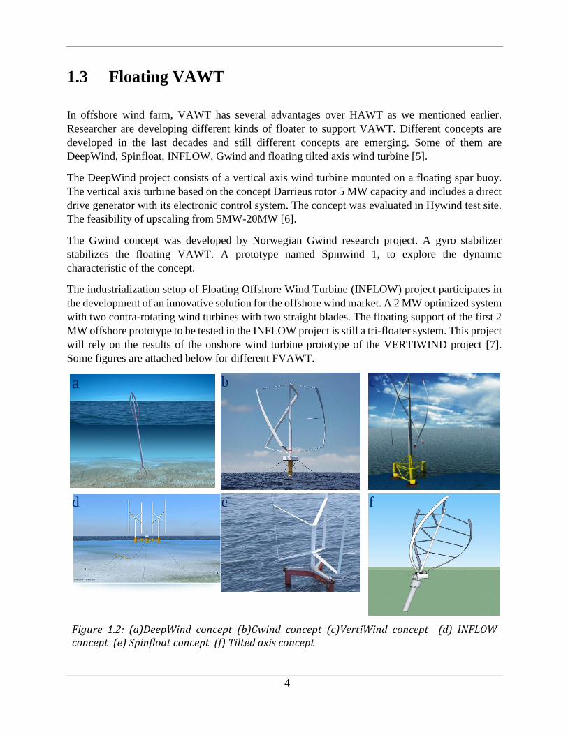
In offshore wind farm, VAWT has several advantages over HAWT as we mentioned earlier.
Researcher are developing different kinds of floater to support VAWT. Different concepts are
developed in the last decades and still different concepts are emerging. Some of them are
DeepWind, Spinfloat, INFLOW, Gwind and floating tilted axis wind turbine [5].
The DeepWind project consists of a vertical axis wind turbine mounted on a floating spar buoy.
The vertical axis turbine based on the concept Darrieus rotor 5 MW capacity and includes a direct
drive generator with its electronic control system. The concept was evaluated in Hywind test site.
The feasibility of upscaling from 5MW-20MW [6].
The Gwind concept was developed by Norwegian Gwind research project. A gyro stabilizer
stabilizes the floating VAWT. A prototype named Spinwind 1, to explore the dynamic
characteristic of the concept.
The industrialization setup of Floating Offshore Wind Turbine (INFLOW) project participates in
the development of an innovative solution for the offshore wind market. A 2 MW optimized system
with two contra-rotating wind turbines with two straight blades. The floating support of the first 2
MW offshore prototype to be tested in the INFLOW project is still a tri-floater system. This project
will rely on the results of the onshore wind turbine prototype of the VERTIWIND project [7].
Some figures are attached below for different FVAWT.
a b c
d e f
Figure 1.2: (a)DeepWind concept (b)Gwind concept (c)VertiWind concept (d) INFLOW concept (e) Spinfloat concept (f) Tilted axis concept

5
1.4 State of art in VAWT and HAWT modelling
We mentioned earlier, HAWTs are the main focus of the wind energy industry, the technology is
more mature than VAWTs. VAWTs lost its ground due to its low efficiency and fatigue issues.
The maximum efficiency a turbine can achieve is 59.3% which is known as Betz limit. HAWTs
are more efficient than VAWTs. The efficiency for HAWTs up to 50% while for VAWTs the
efficiency is approximately 40% [8].
Major driving point to design the floating turbine is the scalability. HAWT have this limitation
due to the gravitational fatigue as the blades undergo tension-compression cycle. As for VAWT
we do not have such problem. HAWTs have gravitational fatigue issues, VAWTs produces
cyclically varying torque that can have adverse effect on transmission and control systems. Due to
the advancement of material technology we can easily solve this problem by using composite
materials [9].
As we discussed earlier, machinery in VAWTs can be handled more effectively than HAWTs. In
VAWTs the machinery placed in the bottom of the tower while for HAWTs the nacelle is placed
at the top of the tower. This is one of the reason the cost for maintenance for HAWTs is higher
than VAWTs.
1.4.1 Aerodynamic modelling
The aerodynamic model used for VAWTs are Blade Element Momentum theory (BEM), Cascade
model, Vortex mode, Actuator Cylinder model (AC). Reynolds-averaged Navier Stokes (RANS)
model and Computational Fluid Dynamics (CFD) used very complicated and computationally
intensive method.
BEM is used to calculate the load acting on the wind turbines blade. This theory combines both
blade element theory and momentum theory. The first momentum model for VAWTs was
developed by Templin, where a single streamtube passing through an actuator disk to represent
VAWT. Wilson and Lissaman developed the multi streamtube model. The DMS model is one of
the most used model to calculate the aerodynamic loads on the wind turbine. [8].
Cascade model was first developed by Hirsch and Mandal to apply the cascade principal to analyze
the VAWTs. To improve the analytical capability of this model, Mandal and Burton use dynamic
stall and streamline curvature in the model. This model demands more computational time than
momentum model but it gives more accurate results for both low and high solidity rotors [10].
Vortex model assumes potential flow. The velocity field obtain by calculating the influence of
vorticity in the wakes of the blades. Larsen [11] proposed a 2D vortex model and advanced by
Fanucci and Walter [12], Holmes [13] and Wilson [14] Their model assumes high tip speed ratio,
lightly loaded rotor, small angle of attack to ignore stall. These assumption limits the applicability
of the model. The first versatile 3D vortex model was proposed by Strickland et al [15]. Later

6
Strickland employed dynamic effects, dynamic stall model, pitching circulation and added mass
in the model. To accelerate the model Cardona [16] proposed a flow curvature as well as modifying
the dynamic stall model.
The AC model is a quasi-static Eulerian model. The AC model was first developed from the PhD
study carried by Madsen et al. [17]. The basic idea is to use the known AD flow model from
HAWT and to develop a general approach of an actuator surface coinciding with the swept area of
the actual turbine [17]. For a straight bladed VAWT the swept surface area is cylindrical. To reduce
the complexity of the model this model is a 2D representation of the general model.
1.4.2 Couple analysis tool
To this date, several coupled analysis tools were developed for FVAWT. Some of them are
CARDAAX was developed by Paraschivoiu [18] who implemented the DMS model to carry out
the VAWT analysis [8].
Strickland [19] developed two and three-dimensional vortex model VDART2 and VDART3 in
1970s as a part of Sandia National Laboratories effort to develop an analysis tool for VAWT.
While Dixon [20] developed three-dimensional unsteady panel model in Delft University of
Technology and the name of the code is UMPM (Unsteady free wake Multi-Body Panel Method)
[8].
SIMO-RIFLEX-AC and SIMO-RIFLEX-DMS was developed by NTNU. The former one was
developed by Cheng et al. [21] in his thesis while the later one was developed by Wang et al. to
perform the fully coupled analysis for floating VAWTs. In this study, we use actuator cylinder
model to calculate the aerodynamic loads on the wind turbine. The code was based on the work of
Madsen et al. [17] while doing his Ph.D. thesis. The code was then coupled with SIMO and
RIFLEX. It integrates the aerodynamic loads, hydrodynamic loads, structural dynamics, control
system and mooring dynamics in a fully coupled way. The hydrodynamic loads are calculated by
the SIMO where it considers the platform as rigid body. The hydrodynamic loads are calculated
based on potential flow theory and Morison’s model for slender body. The tower, shaft, mooring
lines which are designed as flexible finite elements, are solved by using non-linear FEM solver.
While calculating the aerodynamic loads on the wind turbine based on AC method, it also
considers the shear effect of wind and Beddoes-Leishman dynamic stall model. A generator torque
controller was also implemented to regulate the rotor rotational speed based on the PI algorithm
[5].
HAWC2 also apply the AC method to calculate the aerodynamic loads on VAWTs. HAWC2 was
originally developed for the couple analysis of HAWTs, later developed for VAWTs [22]. This
software was developed DTU. To calculate the hydrodynamic loads on the platform it uses
Morison equation and coupling with WAMIT [5].
Beside that some available tools used to analyze the VAWTs are OWENS (Offshore Wind Energy
Simulation), developed by Sandia National Laboratories, CALHYPSO (Calcul Hydrodynamique

7
Poer les Structures Offshore), FloVAWT (Floating Vertical Axis Wind Turbine) developed by
Cranfield University [5].
1.5 Aim and scope of the study
The purpose of this thesis is to design a OC4 semi-submersible offshore platform that will
support a 5 MW vertical axis wind turbine. For this reason, a coupled analysis was
developed in SIMO-RIFLEX-AC to observe the global response of the total system. The central
focus of this thesis to observe the response in different wind and wave conditions. Also, we
need to carefully select the principal parameter of the platform that will preserve the total
stability of the system. Then the optimized system which is developed in this study need to be
compared with the old OC4 semi-submersible. The basic task that will address in this study are
the following:
Based on the design of the semi-submersible from the project work, establish a time domain
model in SIMO-RIFLEX-AC using the wind turbine model from the old OC4
concept. Care should be given to the adjustment of the mass and restoring matrix
when the tower and the blades are modelled explicitly as RIFLEX beams. This topic will
be address in chapter two and three.
Perform decay tests to identify the natural periods and damping coefficients for the
rigid-body motion modes. This topic will be discussed in chapter two.
Perform time-domain simulations for the turbulent wind and irregular wave
cases and compare the statistics and the spectra for the dynamic responses of the new
semi-submersible wind turbine and the old OC4 wind turbine. This topic will be addressed
in chapter three.
Two analyze the second order drift effect on the system and then compare the difference
in the first order prediction. This topic will be discussed on chapter four.
8
Chapter 2
Design and stability of Floating semi-submersible
2.1 Platform design
The design of a floating VAWT is pushed by two basic parameters:
Structural integrity of the body.
Static and dynamic stability of the body.
The total body comprised of two basic structure. The first one is OC4 semi-submersible and the
second one is wind turbine. To float the wind turbine in this study, we designed a OC4 semi-
submersible. Within the framework of OC4 (Offshore Code Comparison Collaboration,
Continuation) projects, hydrodynamic calculation and code to code comparison were performed
for NREL 5 MW wind turbine on top of the DeepCwind semi-submersible platform [23].
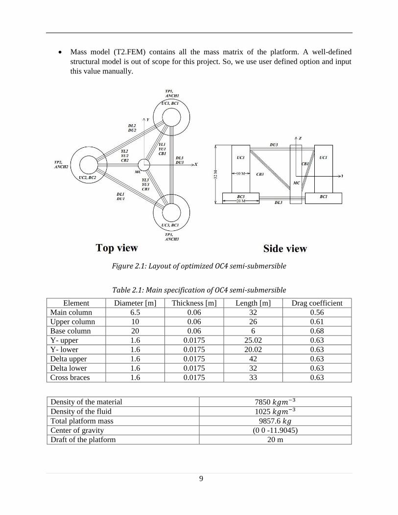
The DeepCwind semi-submersible is designed for 200 m depth, consists of one main column (MC)
and three offset column (OC). On top of the main column, the 5MW wind turbine rested. Each
offset column is divided into two parts. One upper column (UC) and the other one is known as
base column (BC). The base column has larger diameter than the upper column. It also represents
a heave plate which acted as suppression device. The center of the offset column arranged on top
of an equilateral triangle whose edge length is 52 m. Offset column and main column are connected
by braces and pontoons. Cross braces (CB) are connected to the bottom of the main column and
pontoon are used to connect the offset and main column. Pontoons are divided into delta and Y
pontoons. They are named due to their arrangement as seen from the figure. The upper and lower
Y pontoon (YU and YL) are connected to main and offset column while the upper and lower delta
are interconnected to the offset column (DU and DL). Before discussing on the stability, it’s
necessary to introduce the method of developing panel model in HydroD and the model.
To analyze the stability of the platform we first need to build a panel model for HydroD. The first
task is to develop a FEM model in GeniE. As it involves a lot of iteration, in the first step, we
create a parametric model in GeniE and by changing the parameter we can easily build a new
platform. The principal step is listed below:
Panel model (T1.FEM) which have distinctive wetted surface define by GeniE and import
in HydroD to calculate hydrostatic pressure and measure the buoyancy force. A panel
model for a DeepCwind is shown in the following figure.
9
Mass model (T2.FEM) contains all the mass matrix of the platform. A well-defined
structural model is out of scope for this project. So, we use user defined option and input
this value manually.
Figure 2.1: Layout of optimized OC4 semi-submersible
Table 2.1: Main specification of OC4 semi-submersible
Element Diameter [m] Thickness [m] Length [m] Drag coefficient
Main column 6.5 0.06 32 0.56
Upper column 10 0.06 26 0.61
Base column 20 0.06 6 0.68
Y- upper 1.6 0.0175 25.02 0.63
Y- lower 1.6 0.0175 20.02 0.63
Delta upper 1.6 0.0175 42 0.63
Delta lower 1.6 0.0175 32 0.63
Cross braces 1.6 0.0175 33 0.63
Density of the material 7850 𝑘𝑔𝑚−3
Density of the fluid 1025 𝑘𝑔𝑚−3
Total platform mass 9857.6 𝑘𝑔
Center of gravity (0 0 -11.9045)
Draft of the platform 20 m

10
The floating platform is moored with three catenary lines. Each line is 120 apart from each other.
They are used to secure the platform and restraint the movement. Lines are symmetrical about x
axis. Fairleads are located at the top of the base column, at a depth 14 m below the SWL and
connected to the anchor. The anchors are rested on the seabed, 200 m below the SWL. The
following table summarizes all the necessary detail of the mooring lines. Also, the stability results
for the new OC4 semi-submersible will be discussed at end of the this chapter.
Table 2.2: Specification of mooring line
Number of mooring lines 3
Angle between adjacent lines 120 Depth of anchor below SWL 200 m
Depth of fairleads below SWL 14 m
Radius of fairlead from the platform centerline 40.02 m
Radius of anchor from the platform centerline 835.5 m
Mooring line diameter 0.0766 m
Per unit mass density 113.35 kg/m
Hydrodynamic drag coefficient 1.1
Hydrodynamic added mass coefficient 1.0
Structural damping of mooring lines 2.0%
Table 2.3: Principal parameter of straight bladed wind turbine
Rated power [MW] 5.30
Blade number [-] 3
Rotor radius [m] 39
Rotor height [m] 80
Chord length [m] 2.7
Aerofoil section NACA 0018
Tower top height [m] 79.78
Cut in, rated and cut out wind speed [m/s] 5.0, 14.0, 25.0
Rated rotational speed [rad/s] 1.08
Total mass, including rotor, shaft and tower [ton] 315.3
Center of mass for rotor [m] (0, 0, 48.14)
2.2 Old OC4 Platform
One of the main objective of this study is to optimize the characteristic of the OC4 semi-
submersible and compare the data to the old one. In this study, the parent OC4 semi-submersible,
which was our base design and which was designed to support a three-bladed floating VAWT. For
the straight-bladed rotors, the structural properties of the blades, struts, tower and shaft were
determined based on the Deepwind rotor, 5MW Darrieus rotor [24] . The blade used NACA 0018
airfoil. It was assumed that the structural properties of the blades such as mass per unit length,

11
axial and bending stiffness. The blades, instead of struts are our concern [25]. The OC4 semi-
submersible which was originally designed to support the NREL 5 MW wind turbine, was used to
support the three bladed VAWTs. The design was carried out for a depth of 200 m. The same semi-
submersible was used to support the 5MW Darrieus Deepwind rotor and Cheng et.al. (2015b) and
Wang et. al. (2016). Due to difference in weight in the rotor mass, ballast water was adjusted to
maintain the same draft. The properties of the semi-submersible were given below [25]:
Table 2.4: Principal parameter of the original semi-submersible
Parameter Value
Water depth [m] 200
Draft of the platform [m] 20
Diameter at the mean water line (upper column/center column) [m] 10/6.5
Rotor mass, including blades, struts, tower and shaft [ton] 315.3
Center of mass of the rotor [m] (0, 0, 48.14)
Platform mass including ballast and generator [ton] 13796.1
Center of mass for the platform [m] (0, 0, -13.43)
Buoyancy at the equilibrium position [KN] 139816
Center of buoyancy [m] (0, 0, -13.15)
2.3 Fixed VAWT model
One of the objective of this study, to carry out a comparative study with different VAWT model.
Here, we used this model in our study to check the wind turbine performance parameter which will
present in the next chapter. Right now, we just discuss the model. Beside to OC4 semi-submersible
we used landbased VAWT. Three straight bladed fixed wind turbine is studied together with the
OC4 new and old platform. The power output of the landbased wind turbine is 5 MW which used
Darrieus rotor. The structural properties of straight bladed rotor such as structural properties of
blades, struts, tower and shafts were determined based on DeepWind rotor (Vita, 2011) [25]. This
turbine used NACA 0018 airfoil. The structural properties of the wind turbine are assumed to be
same. The stiffness of the blades and struts were increased to avoid large deformation. The stiffness
of the tower and shaft remained same. In a realistic situation, the stiffness of different component
might differ slightly or might add additional struts as shown in the dashed line in the following
figure [25].
As for the floating semi-submersible, we used similar configuration for old and new OC4 floater.
They both support Darrieus 5 MW wind turbine. The figure added describes the arrangement of
the wind turbine where the left one is the landbased wind turbine while the figure in the right side
shows the arrangement of the OC4 semi-submersible both for the old and the new one. The layout
of the optimized OC4 floater and original floater are similar.

12
Figure 2.2: Schematic diagram of ladbased VAWT and OC4 floating VAWT
Table 2.5: Specification of landbased VAWT
Rated power [MW] 5.30
Rotor radius [m] 39.0
Rotor height [m] 80
Chord length [m] 2.7
Tower top height [m] 80.0
Aerofoil section NACA 0018
Cut in, rated and cut out wind speed [m/s] 5.0, 14.0, 25.0
Rated rotor rotational speed [rpm] 1.08
Blade number 3
2.4 Coordinate system
The platform specifications refer to an inertial reference frame and platform DOFs. Three
orthogonal set of axes X, Y and Z are chosen for this purpose. XY plane represent SWL and the
remaining axis projected upward opposite to the gravity which coincide with the platform axis.
The rigid body motion includes three translations and three rotations. Surge, sway and heave are
linear displacement while roll, pitch and yaw are rotational motion. Positive surge defined as along
the positive X axis, positive sway along the positive Y axis and positive heave along positive Z
axis. Positive roll defined along positive X axis, pitch along Y axis and positive yaw along positive
Z axis.

13
Figure 2.3: Coordinate system
2.5 Platform hydrodynamic properties
Hydrodynamic loads include contribution from linear hydrostatics, linear excitation from incident
waves, linear radiation from outgoing waves and non-linear effect such as drift forces[1]. In this
study, we use linear theory of wave to solve the motion equation of the platform. According to this
theory, the performance characteristics of the floating body can be described by the amplitude of
the body as they are linearly related to each other. For this assumption, we can apply superposition
of the effects. The hydrodynamic load on the platform are composed of three different
contributions:
Hydrostatic loads, which exists without any external forces such as wave or wind force.
Buoyancy force which acts through the center of buoyancy according to the law of
Archimedes and weight acting through the center of gravity creates a moment of magnitude
∆.GZ. Here ∆ is the weight displacement and GZ is the righting lever. Restoring force is
also include in the calculation.
Diffraction loads, corresponding to the loads on the body when the body is fixed in an
oscillatory flow. Scattering wave forces and Froude-Krylov forces are closely related to
this category.
Radiation forces occurs when the when the body radiates waves in steady water in a
frequency equals the applied frequency. They are known as added mass and damping of
the floater.
14
2.5.1 Hydrostatic loads
The hydrostatic loads consists of restoring terms and the gravitational term acting along the Z axis.
The total loads on the floating platform from linear hydrostatics,
𝐹𝑖ℎ𝑦𝑑𝑟𝑜
= 𝜌𝑔𝑉0𝛿𝑖3 − 𝐶𝑖𝑗ℎ𝑦𝑑𝑟𝑜
𝑞𝑗 (2.1)
Where, 𝜌 is the density of water, g is the gravitational acceleration, 𝑉0 is the volume displacement
of water, 𝛿𝑖3 is known as Kronecker-Delta function for (i,3) component. 𝐶𝑖𝑗ℎ𝑦𝑑𝑟𝑜
is the (i, j)
component of from the linear hydrostatic restoring matrix from the effects of water plane area and
the center of buoyancy and 𝑞𝑗 is the Jth term of platform DOF[1]. The subscript value in equation
(2.1) ranges from 1-6(1= surge, 2=sway, 3= heave, 4= roll, 5=pitch, 6= yaw) [23].
The first term in the right-hand side of the equation represents the buoyancy force derived from
Archimedes principle which acted vertically upward and the magnitude is equal to the weight of
the displaced water when the platform is in undisplaced position. Only the vertical component of
heave is activated. The second term represents the net change in the hydrostatic forces and
moments when the platform is displaced from its original position. The water density is taken as
1025 𝑘𝑔𝑚−3 .
2.5.2 Hydrodynamics
The hydrodynamic loads associated with excitation forces which includes diffraction waves,
radiated waves from the platform, added mass, viscosity, linear and nonlinear drags. In our study,
we use potential flow theory, which helps us to formulate radiation and diffraction problem.
2.5.3 Potential flow theory
In this system, the flow around the bodies are treated as inviscid, incompressible and irrotational.
This is because the viscous effects are limited to a thin layer next to the body called boundary
layer. We can define the potential function, 𝜑(𝑥, 𝑦, 𝑧, 𝑡) as a continuous function that satisfies the
conservation of mass and momentum.
If 𝜑(𝑥, 𝑦, 𝑧, 𝑡) is scalar quantity then,
𝛻 𝑋 𝛻𝜑 =0 (2.2)
And for irrotational flow,
𝛻 𝑋 �� =0 (2.3)
Therefore, 𝑉 = 𝛻𝜑 and it satisfies the Laplace equation.

15
The linear potential problem is solved in HydroD by using WADAM in the frequency domain
analysis. We had taken sixty components of the frequency and used a 3D panel model to solve the
radiation and the diffraction problem. The solution regarding radiation problem, associated with
oscillation of the platform is given in terms of frequency dependent added mass and damping
matrices, 𝐴𝑖𝑗 and 𝐵𝑖𝑗. The diffraction problem, consider hydrodynamic loads associated with the
incident waves on the platform [23].
In GeniE, we first modelled our platform as a panel and then export the FEM files in the HydroD.
In the first step, we check overall stability of the platform and then run the frequency domain
analysis in WADAM. In the panel model, we adopt 1.2 m as the standard panel size. The semi-
submersible was analyzed into a finite water depth 200 m.
The added mass and damping matrices has the dimension 6x6 for its six degrees of freedom. Due
to the symmetry, the surge-surge elements of the frequency dependent added mass and damping
matrices, 𝐴11 and 𝐵11 are identical to the sway-sway elements 𝐴22 and 𝐵22. Likewise, the roll-roll
elements 𝐴44 𝐵44 are identical to the pitch-pitch elements, 𝐴55 and 𝐵55. The behavior also exists
for the wave heading angle. We get the same response at 0°, 120° and 240° wave headings. The
layout of the design is shown below:
Figure 2.4: Wave heading direction with respect to platform

16
2.6 Morison’s equation
Morison’s formula is applicable for calculating the hydrodynamic loads on cylindrical structure
when three points are fulfilled. They are:
The diffraction effect is negligible.
Radiation damping is negligible.
Flow separation may occur.
The relative form of Morison’s equation accounted form wave-induced excitation, radiation-
induced added mass and flow separation induces viscous drag [23].
2.7 Added mass
Morison’s law is a reasonable approximation for OC4 semi-submersible in most cases because
diffraction effects are negligible in moderate to severe sea states, radiation damping in most cases
is very small. In severe sea states, flow separation might occur is the upper part of the column [23].
For a cylinder in steady transverse flow, the Morison’s equation can be expressed as[4]:
𝐹 =1
2𝐶𝑑𝜌𝐷|𝑢 − 𝑢𝑟|(𝑢 − 𝑢𝑟) +
1
4(1 + 𝐶𝑎)𝜌𝜋𝐷2𝑢 −
1
4
𝜌𝐶𝑎𝜋𝐷2𝑢�� (2.4)
Here, ρ is the density of the fluid, D is the cylinder diameter, u and 𝑎1are the horizontal undisturbed
velocity and acceleration at the midpoint of the strip. The mass and drag coefficients depends on
Reynolds number, Keulegan-Carpenter number, surface roughness ratios and relative current
number. The added mass coefficient 𝐶𝑎 was selected such that 𝐶𝑎𝜌𝑉 is equaled the zero-frequency
limit of 𝐴11 in the surge degree of freedom. The assumption for 𝐶𝑎 is independent of the depth and
the motion is relatively in the low frequency region. 𝑢𝑟 is the cylinder velocity.
For the platform, we use three base columns as heave plate. The force on a heave plate need to
model carefully because the heave plate does not scale proportionally with respect to the displaced
fluid. The hydrodynamic force on heave plate is to be modelled according to the modified
Morison’s equation which mentioned below [23]:
𝐹 =1
2𝐶𝑑𝑧𝜌𝐴𝑐|𝑤 − 𝑢𝑟|(𝑢 − 𝑢𝑟) + 𝜌𝐶𝑎𝑧𝑉𝑟(�� − 𝑢��) +
1
4𝜋𝐷ℎ
2𝑝𝑏 −1
4𝜋(𝐷ℎ
2 − 𝐷𝑐2)𝑝𝑡 (2.5)
Where, 𝐶𝑑𝑧 is drag coefficient in the heave direction, 𝐴𝑐 is the cross-sectional area of the base
column, 𝑤 is the wave particle velocity and 𝑢𝑟 is heave velocity of the base column.𝐶𝑎𝑧 is the
added mass coefficient, 𝑉𝑟 is the reference heave volume, �� is the vertical wave particle
acceleration, 𝑢�� is the vertical acceleration of the base column, 𝐷ℎ is the diameter of the base
column, 𝐷𝑐 is the diameter of the upper column and 𝑝𝑏 , 𝑝𝑡 are the dynamic pressure acting on the
bottom and top faces of the column. The first term represents the drag force in the heave direction,
the second one stands for added mass force and the last two part represents the Froude-Krylov

17
force expressed in terms of pressure. The table shown below essentially summarizes the
hydrodynamic properties of the floating platform:
Table 2.6: Hydrodynamic coefficients
Water density (ρ) 1025 𝑘𝑔𝑚−3
Water depth (h) 200 m
Dispalced water in undisplaced position (𝑉0) 9857.6 ton
Added mass coefficient for all members (𝐶𝑎) 0.63
Drag coefficient for main column (𝐶𝑑) 0.56
Drag coefficient for upper column (𝐶𝑑) 0.61
Drag coefficient for base column (𝐶𝑑) 0.68
Drag coefficient for braces and pontoon (𝐶𝑑) 0.63
Drag coefficient for base column (𝐶𝑑𝑧) 4.80
2.8 Intact Floating Stability Floating stability implies a stable equilibrium and reflection of total integrity against downflooding
and capsizing. Satisfactory floating stability for wind turbine units is necessary to support the
safety level required for the involved structures. The intact stability of the structure is discussed
below:
The wind heeling moment applied in the stability calculation for a wind speed equal to the
wind speed that produces the largest rotor thrust assuming the that the rotor plane is normal
to the direction of flow.
For sufficient stability, also in fault situation that the turbine does not yaw out of the wind
during severe storm conditions, it will be necessary to assume that the rotor plane is
perpendicular to the wind when calculating the wind heeling moment. A wind speed of 36
m/s may be assumed for this situation.
The area under the righting moment curve to the second intercept or down-flooding angle,
whichever is less, shall be equal or greater than 140% of the area under the wind heeling
moment curve to the same limiting angle [26].
Figure 2.5: Righting moment and wind heeling moment curves
18
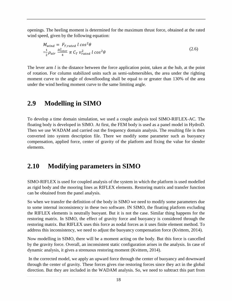
openings. The heeling moment is determined for the maximum thrust force, obtained at the rated
wind speed, given by the following equation:
𝑀𝑤𝑖𝑛𝑑 = 𝐹𝑇,𝑟𝑎𝑡𝑒𝑑 𝑙 𝑐𝑜𝑠2휃
=1
2𝜌𝑎𝑖𝑟
𝐷𝑟𝑜𝑡𝑜𝑟2
4 𝜋 𝐶𝑇 𝑣𝑟𝑎𝑡𝑒𝑑
2 𝑙 𝑐𝑜𝑠2휃 (2.6)
The lever arm 𝑙 is the distance between the force application point, taken at the hub, at the point
of rotation. For column stabilized units such as semi-submersibles, the area under the righting
moment curve to the angle of downflooding shall be equal to or greater than 130% of the area
under the wind heeling moment curve to the same limiting angle.
2.9 Modelling in SIMO
To develop a time domain simulation, we used a couple analysis tool SIMO-RIFLEX-AC. The
floating body is developed in SIMO. At first, the FEM body is used as a panel model in HydroD.
Then we use WADAM and carried out the frequency domain analysis. The resulting file is then
converted into system description file. There we modify some parameter such as buoyancy
compensation, applied force, center of gravity of the platform and fixing the value for slender
elements.
2.10 Modifying parameters in SIMO
SIMO-RIFLEX is used for coupled analysis of the system in which the platform is used modelled
as rigid body and the mooring lines as RIFLEX elements. Restoring matrix and transfer function
can be obtained from the panel analysis.
So when we transfer the definition of the body in SIMO we need to modify some parameters due
to some internal inconsistency in these two software. IN SIMO, the floating platform excluding
the RIFLEX elements is neutrally buoyant. But it is not the case. Similar thing happens for the
restoring matrix. In SIMO, the effect of gravity force and buoyancy is considered through the
restoring matrix. But RIFLEX uses this force as nodal forces as it uses finite element method. To
address this inconsistency, we need to adjust the buoyancy compensation force (Kvittem, 2014).
Now modelling in SIMO, there will be a moment acting on the body. But this force is cancelled
by the gravity force. Overall, an inconsistent static configuration arises in the analysis. In case of
dynamic analysis, it gives a strenuous restoring moment (Kvittem, 2014).
In the corrected model, we apply an upward force through the center of buoyancy and downward
through the center of gravity. These forces gives rise restoring forces since they act in the global
direction. But they are included in the WADAM analysis. So, we need to subtract this part from

19
the restoring matrix. This method effectively then includes only the water plane stiffness. The
procedure is described below:
1. In the Simo description file, we modified the following things:
In the ‘BODY MASS DATA’ section, we used the COG value of the platform
without considering wind turbine.
In the ‘MASS COEFFICIENTS’ section, we used the COG value of the platform
without considering wind turbine.
In the ‘LINEAR STIFFNESS MATRIX’ SECTION I used the following formula:
𝐶44𝑛𝑒𝑤 = 𝐶44
𝑤𝑎𝑑𝑎𝑚 − 𝜌𝑔𝑉0𝑧𝑏 + 𝑚𝑔𝑧𝑔 = 𝟏𝟏𝟏𝟎𝟕𝟐𝟗. 𝟕𝟔𝟖
(2.7) 𝐶55
𝑛𝑒𝑤 = 𝐶55𝑤𝑎𝑑𝑎𝑚 − 𝜌𝑔𝑉0𝑧𝑏 + 𝑚𝑔𝑧𝑔 = 𝟏𝟏𝟏𝟎𝟕𝟐𝟗. 𝟕𝟔𝟖
𝐶46𝑛𝑒𝑤 = 𝐶46
𝑤𝑎𝑑𝑎𝑚 − 𝜌𝑔𝑉0𝑥𝑏 + 𝑚𝑔𝑥𝑔 = 𝐶46𝑤𝑎𝑑𝑎𝑚
𝐶56𝑛𝑒𝑤 = 𝐶56
𝑤𝑎𝑑𝑎𝑚 − 𝜌𝑔𝑉0𝑥𝑏 + 𝑚𝑔𝑥𝑔 = 𝐶56𝑤𝑎𝑑𝑎𝑚
where 𝑉0 is the displaced volume of the body (platform), m is the mass of the
platform with turbine, (𝑥𝑏 , 𝑦𝑏,𝑧𝑏) are the buoyancy location in the global coordinate
system and (𝑥𝑔, 𝑦𝑔,𝑧𝑔) are center of gravity location in the global coordinate
system.
2. In the specified force section, we modified the following things:
‘Gravity of the floater without the brace’ section we consider the mass of the
platform and then multiplied with 9.80665 which gives 93578 KN.
‘Buoyancy of the floater without the brace’ section we consider the buoyancy of the
whole body (Platform+Turbine). The buoyancy force is 96670.516 KN.
2.11 Equation of motion and natural periods
Applying Newton’s second law and considering the applied load, the equation of motion for a
floating object is given by:
𝐹𝑖𝑒−𝑖𝜉𝑡 = ∑[(𝑀𝑖𝑗 + 𝐴𝑖𝑗)
𝑑2휂𝑗
𝑑𝑡2+ 𝐵𝑖𝑗
𝑑휂𝑗
𝑑𝑡+ 𝐶𝑖𝑗휂𝑗] (𝑖 = 1 − 6)
6
𝑗=1
(2.8)
The left term in the equation, represents the external exciting force say wave induced loads or wind
loads. 𝑀𝑖𝑗 is the mass matrix and the body is symmetric about the XZ plane. So, the mass matrix
is given in the following form:
20
𝑀𝑖𝑗 =
[
𝑀 0 0 0 𝑀𝑧𝐺 00 𝑀 0 −𝑀𝑧𝐺 0 00 0 𝑀 0 0 00 −𝑀𝑧𝐺 0 𝐼𝑥 0 −𝐼𝑥𝑧
𝑀𝑧𝐺 0 0 0 𝐼𝑦 0
0 0 0 −𝐼𝑥𝑧 0 𝐼𝑧 ]
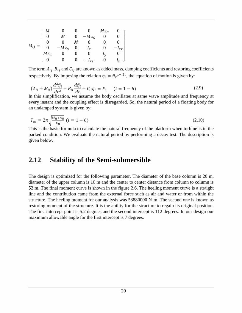
The term 𝐴𝑖𝑗 , 𝐵𝑖𝑗 and 𝐶𝑖𝑗 are known as added mass, damping coefficients and restoring coefficients
respectively. By imposing the relation 휂𝑖 = 휂𝑖𝑒−𝑖𝜉𝑡, the equation of motion is given by:
(𝐴𝑖𝑖 + 𝑀𝑖𝑖)𝑑2휂𝑖
𝑑𝑡2+ 𝐵𝑖𝑖
𝑑휂𝑖
𝑑𝑡+ 𝐶𝑖𝑖휂𝑖 = 𝐹𝑖 (𝑖 = 1 − 6) (2.9)
In this simplification, we assume the body oscillates at same wave amplitude and frequency at
every instant and the coupling effect is disregarded. So, the natural period of a floating body for
an undamped system is given by:
𝑇𝑛𝑖 = 2𝜋√𝑀𝑖𝑖+𝐴𝑖𝑖
𝐶𝑖𝑖 (𝑖 = 1 − 6) (2.10)
This is the basic formula to calculate the natural frequency of the platform when turbine is in the
parked condition. We evaluate the natural period by performing a decay test. The description is
given below.
2.12 Stability of the Semi-submersible
The design is optimized for the following parameter. The diameter of the base column is 20 m,
diameter of the upper column is 10 m and the center to center distance from column to column is
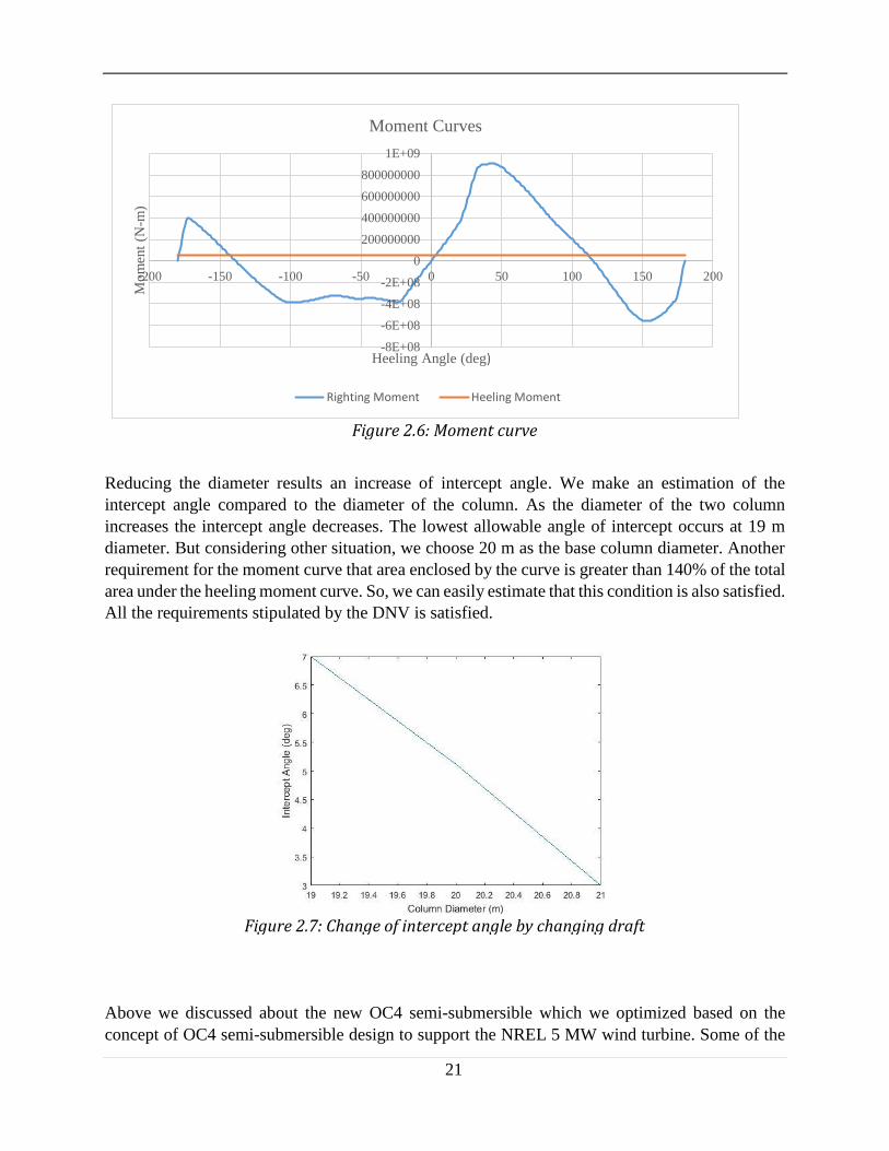
52 m. The final moment curve is shown in the figure 2.6. The heeling moment curve is a straight
line and the contribution came from the external force such as air and water or from within the
structure. The heeling moment for our analysis was 53880000 N-m. The second one is known as
restoring moment of the structure. It is the ability for the structure to regain its original position.
The first intercept point is 5.2 degrees and the second intercept is 112 degrees. In our design our
maximum allowable angle for the first intercept is 7 degrees.
21
Figure 2.6: Moment curve
Reducing the diameter results an increase of intercept angle. We make an estimation of the
intercept angle compared to the diameter of the column. As the diameter of the two column
increases the intercept angle decreases. The lowest allowable angle of intercept occurs at 19 m
diameter. But considering other situation, we choose 20 m as the base column diameter. Another
requirement for the moment curve that area enclosed by the curve is greater than 140% of the total
area under the heeling moment curve. So, we can easily estimate that this condition is also satisfied.
All the requirements stipulated by the DNV is satisfied.
Figure 2.7: Change of intercept angle by changing draft
Above we discussed about the new OC4 semi-submersible which we optimized based on the
concept of OC4 semi-submersible design to support the NREL 5 MW wind turbine. Some of the
-8E+08
-6E+08
-4E+08
-2E+08
0
200000000
400000000
600000000
800000000
1E+09
-200 -150 -100 -50 0 50 100 150 200
Mo
men
t (N
-m)
Heeling Angle (deg)
Moment Curves
Righting Moment Heeling Moment

22
analysis was carried out in my project work. The OC4 semi-submersible is optimized on the basis
of following parameters such as weight and principal parameters without altering the behavior of
the sei-submersible. We are able to reduce the weight significantly and designed in a way which
cleverly adjust the natural frequency outside the range of wave excitation.
23
Chapter 3
Aerodynamic & Hydrodynamic loads on VAWT
3.1 Overview of Aerodynamic Models for FVAWT
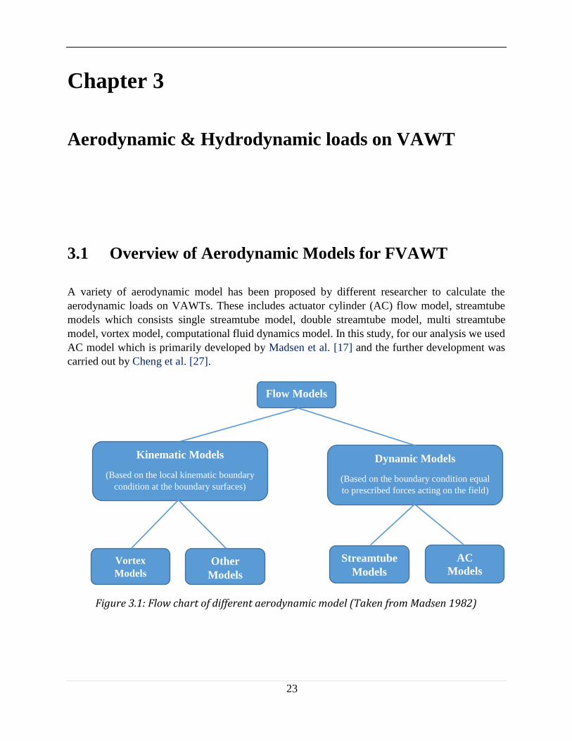
A variety of aerodynamic model has been proposed by different researcher to calculate the
aerodynamic loads on VAWTs. These includes actuator cylinder (AC) flow model, streamtube
models which consists single streamtube model, double streamtube model, multi streamtube
model, vortex model, computational fluid dynamics model. In this study, for our analysis we used
AC model which is primarily developed by Madsen et al. [17] and the further development was
carried out by Cheng et al. [27].
Figure 3.1: Flow chart of different aerodynamic model (Taken from Madsen 1982)
Flow Models
Kinematic Models
(Based on the local kinematic boundary
condition at the boundary surfaces)
Dynamic Models
(Based on the boundary condition equal
to prescribed forces acting on the field)
Vortex
Models
Other
Models
Streamtube
Models
AC
Models

24
3.2 The Actuator Cylinder Flow Model
The AC model was first developed from the PhD study carried by Madsen et al. [17]. The basic
idea to use the known AD (Actuator Disc) flow model from HAWT and to develop a general
approach of an actuator surface coinciding with the swept area of the actual turbine [17]. For a
straight bladed VAWT the swept surface area is cylindrical. To reduce the complexity of the model
this model is a 2D representation of the general model.
The AC model is a quasi-static Eulerian model. The normal and the tangential forces Qn and Qt
resulting from the blade forces are applied on the flow as volume force perpendicular and
tangential to the rotor plane as shown in the figure 3.2.
Figure 3.2: Actuator cylinder model [24]
Our task is to determine the flow field under the disturbance of the external volume forces. The
volume forces fx, uniform and parallel to the free stream velocity V∞. If the drag force is D per unit
length and the velocity, V∞(1-a), then applying momentum theory [17],
D = 2 x2R x ρ𝑉∞2(1 − 𝑎)𝑎 (3.1)
And the drag force D and fx are connected by
lim𝑛→0
∫ 𝑓𝑥𝑛
−𝑛𝑑𝑥 = 2𝑅. 𝑄𝑥 = -D (3.2)

25
From eq. (2) a pressure jump ∆p, when passing through the disc, where ∆p is given by,
∆p = 𝐷
2𝑅= −𝑄𝑥
Radial volume forces are distributed on a cylindrical surface and will thus create a pressure jump,
∆p across the surface.
∆p = lim𝑛→0
∫ 𝑓𝑟(휃)𝑅+𝑛
𝑅−𝑛
𝑑𝑟 = 𝑄𝑟(휃) (3.3)
The power extracted from the fluid per unit length of the cylinder is given by
P𝑖𝑑𝑒𝑎𝑙 = ∫ 𝑉𝑟(휃). ∆𝑝(휃)2𝜋
0. 𝑅𝑑휃 (3.4)
And the power coefficient is given by
C𝑝,𝑖𝑑𝑒𝑎𝑙 = 𝑃
12 𝜌𝑉∞
3. 2𝑅=
∫ 𝑉𝑟(휃). ∆𝑝(휃)2𝜋
0. 𝑅𝑑휃
12 𝜌𝑉∞
3. 2𝑅 (3.5)
Finally, the extracted power by the turbine and its power coefficient are defined by the following
equations
P = 1
2𝜋∫ 𝑁 𝐹𝑡(휃). 𝛺
2𝜋
0. 𝑅𝑑휃 (3.6)
and
C𝑝 = 𝑃
12 𝜌𝑉∞
3. 2𝑅=
12𝜋 ∫ 𝑁 𝐹𝑡(휃). 𝛺
2𝜋
0. 𝑅𝑑휃
12 𝜌𝑉∞
3. 2𝑅 (3.7)
3.2.1 Governing equations and method of solution
The basic equations and solution method described by Madsen et al. [17] will be described briefly.
The basic equation for the 2D case is the Euler equation. Suppose the velocity components are 𝑣𝑥
and 𝑣𝑦 can be written as,
𝑣𝑥 = 1 + 𝑤𝑥 and 𝑣𝑦 = 𝑤𝑦 (3.8)
Now the Euler equations takes the form:
𝜕𝑤𝑥
𝜕𝑥+ 𝑤𝑥
𝜕𝑤𝑥
𝜕𝑥+ 𝑤𝑦
𝜕𝑤𝑥
𝜕𝑦= −
𝜕p
𝜕𝑥+ 𝑓𝑥
(3.9)
𝜕𝑤𝑦
𝜕𝑥+ 𝑤𝑥
𝜕𝑤𝑦
𝜕𝑥+ 𝑤𝑦
𝜕𝑤𝑦
𝜕𝑦= −
𝜕p
𝜕𝑦+ 𝑓𝑦 (3.10)
and the continuity equation is given by

26
𝜕𝑤𝑥
𝜕𝑥+
𝜕𝑤𝑦
𝜕𝑦= 0 (3.11)
Where p is the pressure and f is the volume forces.
The value of 𝑄𝑛(휃) and 𝑄𝑡(휃) derived from the blade forces per unit length by the following
equations:
𝑄𝑛(휃) = 𝐵𝐹𝑛 휃
2𝜋𝑅𝜌𝑉∞2
(3.12)
𝑄𝑡(휃) = 𝐵𝐹𝑡 휃
2𝜋𝑅𝜌𝑉∞2 (3.13)
Where B is the blade number and R is the radius of blade path.
Equation (9) and (10) can be rewritten as:
𝜕𝑤𝑥
𝜕𝑥= −
𝜕p
𝜕𝑥+ 𝑓𝑥 + 𝑔𝑥
(3.14) 𝜕𝑤𝑥
𝜕𝑦= −
𝜕p
𝜕𝑦+ 𝑓𝑦 + 𝑔𝑦
Where 𝑔𝑥 and 𝑔𝑦 are second order forces:
𝑔𝑥 = −(𝑤𝑥
𝜕𝑤𝑥
𝜕𝑥+ 𝑤𝑦
𝜕𝑤𝑥
𝜕𝑦)
(3.15)
𝑔𝑦 = −(𝑤𝑥
𝜕𝑤𝑦
𝜕𝑥+ 𝑤𝑦
𝜕𝑤𝑦
𝜕𝑦)
So, the final equation for the pressure:
𝜕2𝑝
𝜕𝑥2+
𝜕2𝑝
𝜕𝑦2= (
𝜕𝑓𝑥𝜕𝑥
+𝜕𝑓𝑦
𝜕𝑦) + (
𝜕𝑔𝑥
𝜕𝑥+
𝜕𝑔𝑦
𝜕𝑦) (3.16)
Which is Poisson type equation.
The solution of this equation with the appropriate boundary conditions 𝑝 → 0 and 𝑥, 𝑦 → ∞ can
be written as:
𝑝(𝑓) = 1
2𝜋 ∬
𝑓𝑥(𝑥 − 𝜉) + 𝑓𝑦(𝑦 − 휂)
(𝑥 − 𝜉)2 + (𝑦 − 휂)2 𝑑𝜉𝑑휂
(3.17)
𝑝(𝑔) = 1
2𝜋 ∬
𝑔𝑥(𝑥 − 𝜉) + 𝑔𝑦(𝑦 − 휂)
(𝑥 − 𝜉)2 + (𝑦 − 휂)2 𝑑𝜉𝑑휂 (3.18)

27
Once the pressure field is found the velocities can be determined by equation 3.19 and 3.20.
𝑤𝑥 = −𝑝(𝑓) + 𝐼𝑓𝑥 − 𝑝(𝑔) + 𝐼𝑔𝑥 = 𝑤𝑥(𝑓) + 𝑤𝑥(𝑔) (3.19)
𝑤𝑦 = ∬𝜕
𝜕𝑥𝑝(𝑓)𝑑𝑥′
𝑥
−∞
+ 𝐼𝑓𝑦 − ∬𝜕
𝜕𝑦𝑝(𝑔)𝑑𝑥′
𝑥
−∞
+ 𝐼𝑔𝑦 = 𝑤𝑥(𝑓) + 𝑤𝑥(𝑔) (3.20)
Where, 𝐼𝑓𝑥 = ∫ 𝑓𝑥𝑑𝑥′𝑥
−∞
𝐼𝑓𝑦 = ∫ 𝑓𝑦𝑑𝑥′𝑥
−∞
𝐼𝑔𝑥 = ∫ 𝑔𝑥𝑑𝑥′𝑥
−∞
𝐼𝑔𝑦 = ∫ 𝑔𝑦𝑑𝑥′𝑥
−∞
The final solution can be written as a sum of two parts. One is linear and the other part is nonlinear.
An important characteristic for the solution as the prescribed forces only applied on a circle, so the
pressure solution for the linear part become the solution of Laplace equation in two connected
regions; outside the cylinder and inside the cylinder[8].
3.2.2 Linear Solution
For the normal loading on the AC which is the largest force than tangential force, the linear solution
can be worked out [27]:
𝑤𝑥 = −1
2𝜋∫ 𝑄𝑛(휃)
−(𝑥+sin𝜃) sin𝜃+(𝑦−cos𝜃) cos𝜃
(𝑥+sin𝜃)2+(𝑦−cos𝜃)2𝑑휃 −
2𝜋
0
1
2𝜋∫ 𝑄𝑡(휃)
−(𝑥+sin𝜃) cos𝜃−(𝑦−cos𝜃) sin𝜃
(𝑥+sin𝜃)2+(𝑦−cos𝜃)2𝑑휃 −
2𝜋
0 (𝑄𝑛 (cos−1 𝑦))∗ +
(𝑄𝑛 (−cos−1 𝑦))∗∗ − (𝑄𝑡 (cos−1 𝑦)𝑦
√1−𝑦2)
∗
− (𝑄𝑡 (−cos−1 𝑦)𝑦
√1−𝑦2)
∗∗
(3.21)
𝑤𝑦 = −1
2𝜋∫ 𝑄𝑛(휃)
−(𝑥 + sin 휃) cos 휃 + (𝑦 − cos 휃) sin 휃
(𝑥 + sin 휃)2 + (𝑦 − cos 휃)2𝑑휃
2𝜋
0
−1
2𝜋∫ 𝑄𝑡(휃)
(𝑥 + sin 휃) sin 휃 − (𝑦 − cos 휃) cos 휃
(𝑥 + sin 휃)2 + (𝑦 − cos 휃)2𝑑휃
2𝜋
0
(3.22)
The term marked with * in equation 3.21 shall be added inside the cylinder and in case wake behind
the cylinder both the term marked with * and ** shall be included. It is to be noted that the original
work of Madsen et al. [17] does not include the tangential terms but in the work of Cheng et al.
[27] this term is included.

28
Assuming the loading is piecewise constant we can derive from equation (3.21) and (3.22):
𝑤𝑥 = −1
2𝜋∑𝑄𝑛,𝑖 ∫
−(𝑥 + sin 휃) sin 휃 + (𝑦 − cos 휃) cos 휃
(𝑥 + sin 휃)2 + (𝑦 − cos 휃)2𝑑휃
𝜃𝑖+12∆𝜃
𝜃𝑖−12∆𝜃
𝑖=𝑁
𝑖=1
−1
2𝜋∑ 𝑄𝑡,𝑖 ∫
−(𝑥 + sin 휃) cos 휃 + (𝑦 − cos 휃) sin 휃
(𝑥 + sin 휃)2 + (𝑦 − cos 휃)2𝑑휃
𝜃𝑖+12∆𝜃
𝜃𝑖−12∆𝜃
𝑖=𝑁
𝑖=1
(3.23)
𝑤𝑦 = −1
2𝜋∑ 𝑄𝑛,𝑖 ∫
−(𝑥 + sin 휃) cos 휃 + (𝑦 − cos 휃) sin 휃
(𝑥 + sin 휃)2 + (𝑦 − cos 휃)2𝑑휃
𝜃𝑖+12∆𝜃
𝜃𝑖−12∆𝜃
𝑖=𝑁
𝑖=1
+1
2𝜋∑ 𝑄𝑡,𝑖 ∫
−(𝑥 + sin 휃) sin 휃 + (𝑦 − cos 휃) cos 휃
(𝑥 + sin 휃)2 + (𝑦 − cos 휃)2𝑑휃
𝜃𝑖+12∆𝜃
𝜃𝑖−12∆𝜃
𝑖=𝑁
𝑖=1
(3.24)
Where N is the total number of calculation points, ∆θ =2𝜋
𝑁 and 휃𝑖 =
𝜋
𝑁(2𝑖 − 1) for 𝑖 =
1,2,3… . . 𝑁.
Only the induced velocity at the cylinder are of concern, the total velocity solution at calculation
point (𝑥𝑗, 𝑦𝑗) on the cylinder can then be written as:
𝑤𝑥,𝑗 = −1
2𝜋(∑ 𝑄𝑛,𝑖𝐼1,𝑖,𝑗
𝑖=𝑁
𝑖=1
+ ∑ 𝑄𝑡,𝑖𝐼2,𝑖,𝑗
𝑖=𝑁
𝑖=1
) − (𝑄𝑛,𝑁+1−𝑗)∗−
(
𝑄𝑡,𝑁+1−𝑗
𝑦𝑗
√1 − 𝑦𝑗2
)
∗
(3.25)
𝑤𝑥,𝑗 = −1
2𝜋(∑ 𝑄𝑛,𝑖𝐼2,𝑖,𝑗
𝑖=𝑁
𝑖=1
+ ∑ 𝑄𝑡,𝑖𝐼1,𝑖,𝑗
𝑖=𝑁
𝑖=1
) (3.26)
Where the terms marked with * in equation (25) and (26) are only added for 𝑗 =𝑁
2
𝐼1,𝑖,𝑗 and 𝐼2,𝑖,𝑗 are influenced coefficients in point j influenced by another point I are given by
𝐼1,𝑖,𝑗 = ∫−(𝑥𝑗 + sin 휃) sin 휃 + (𝑦𝑗 − cos 휃) cos 휃
(𝑥𝑗 + sin 휃)2+ (𝑦𝑗 − cos 휃)
2 𝑑휃𝜃𝑖+
12∆𝜃
𝜃𝑖−12∆𝜃
(3.27)
𝐼2,𝑖,𝑗 = ∫−(𝑥𝑗 + sin 휃) cos 휃 + (𝑦𝑗 − cos 휃) sin 휃
(𝑥𝑗 + sin 휃)2+ (𝑦𝑗 − cos 휃)
2 𝑑휃𝜃𝑖+
12∆𝜃
𝜃𝑖−12∆𝜃
(3.28)
Where 𝑥𝑗 = −sin( 𝑗∆θ −1
2∆θ), 𝑦𝑗 =cos(𝑗∆θ −
1
2∆θ)
29
3.2.3 Modified Linear Solution
To compute the non-linear solution directly, it takes time. To make the solution in better agreement
with the non-linear solution, a correction was proposed by Madsen et al. [17]. Madsen suggested
to multiply the velocities from the linear solution 𝑤𝑥 and 𝑤𝑦 with the factor:
𝐾𝑎 = 1
1 − 𝑎
But according to Cheng et al. [27] that the correction proposed by Madsen et al. can give some
deviation in the power coefficient at high tip speed ratios when compared to the experimental data.
The modified 𝐾𝑎:
𝐾𝑎 = {
1
1 − 𝑎, 𝑎 ≤ 0.15
1
1 − 𝑎 (0.65 + 0.35exp (−4.5(𝑎 − 0.15))), 𝑎 > 0.15
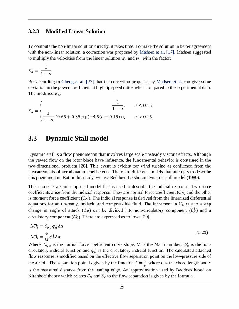
3.3 Dynamic Stall model
Dynamic stall is a flow phenomenon that involves large scale unsteady viscous effects. Although
the yawed flow on the rotor blade have influence, the fundamental behavior is contained in the
two-dimensional problem [28]. This event is evident for wind turbine as confirmed from the
measurements of aerodynamic coefficients. There are different models that attempts to describe
this phenomenon. But in this study, we use Beddoes-Leishman dynamic stall model (1989).
This model is a semi empirical model that is used to describe the indicial response. Two force
coefficients arise from the indicial response. They are normal force coefficient (CN) and the other
is moment force coefficient (CM). The indicial response is derived from the linearized differential
equations for an unsteady, inviscid and compressible fluid. The increment in CN due to a step
change in angle of attack (∆α) can be divided into non-circulatory component (𝐶𝑁𝑙 ) and a
circulatory component (𝐶𝑁𝑐 ). There are expressed as follows [29]:
∆𝐶𝑁𝑐 = 𝐶𝑁𝛼𝜙𝛼
𝐶∆𝛼
(3.29) ∆𝐶𝑁
𝑙 =4
𝑀𝜙𝛼
𝑙 ∆𝛼
Where, 𝐶𝑁𝛼 is the normal force coefficient curve slope, M is the Mach number, 𝜙𝛼𝑙 is the non-
circulatory indicial function and 𝜙𝛼𝑐 is the circulatory indicial function. The calculated attached
flow response is modified based on the effective flow separation point on the low-pressure side of
the airfoil. The separation point is given by the function 𝑓 =𝑥
𝑐 where c is the chord length and x
is the measured distance from the leading edge. An approximation used by Beddoes based on
Kirchhoff theory which relates 𝐶𝑁 and 𝐶𝑐 to the flow separation is given by the formula.
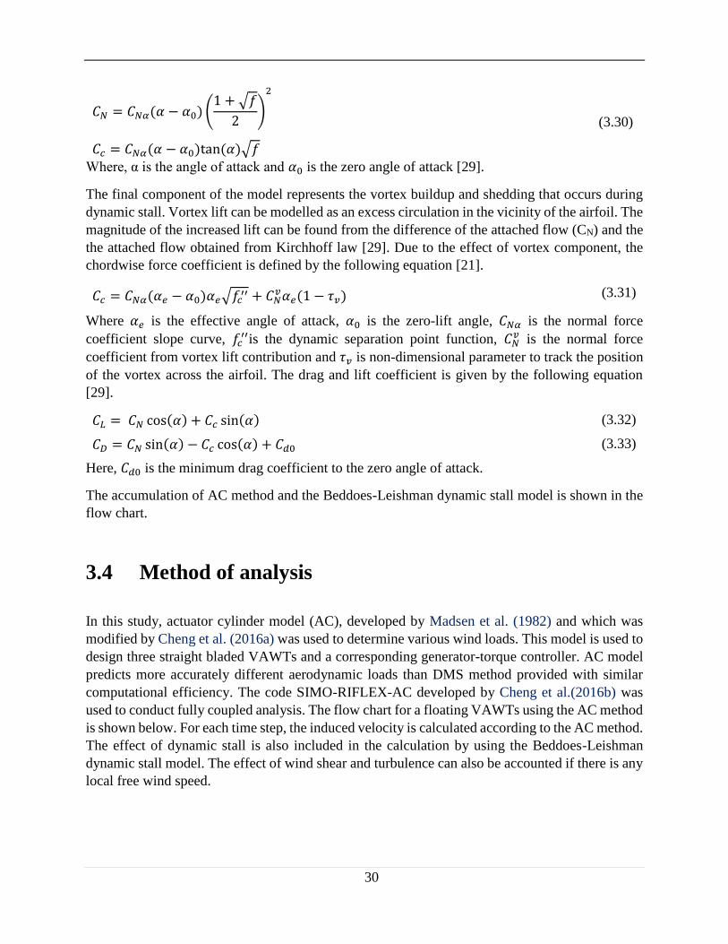
30
𝐶𝑁 = 𝐶𝑁𝛼(𝛼 − 𝛼0) (1 + √𝑓
2)
2
(3.30)
𝐶𝑐 = 𝐶𝑁𝛼(𝛼 − 𝛼0)tan (𝛼)√𝑓
Where, α is the angle of attack and 𝛼0 is the zero angle of attack [29].
The final component of the model represents the vortex buildup and shedding that occurs during
dynamic stall. Vortex lift can be modelled as an excess circulation in the vicinity of the airfoil. The
magnitude of the increased lift can be found from the difference of the attached flow (CN) and the
the attached flow obtained from Kirchhoff law [29]. Due to the effect of vortex component, the
chordwise force coefficient is defined by the following equation [21].
𝐶𝑐 = 𝐶𝑁𝛼(𝛼𝑒 − 𝛼0)𝛼𝑒√𝑓𝑐′′ + 𝐶𝑁𝑣𝛼𝑒(1 − 𝜏𝑣) (3.31)
Where 𝛼𝑒 is the effective angle of attack, 𝛼0 is the zero-lift angle, 𝐶𝑁𝛼 is the normal force
coefficient slope curve, 𝑓𝑐′′is the dynamic separation point function, 𝐶𝑁
𝑣 is the normal force
coefficient from vortex lift contribution and 𝜏𝑣 is non-dimensional parameter to track the position
of the vortex across the airfoil. The drag and lift coefficient is given by the following equation
[29].
𝐶𝐿 = 𝐶𝑁 cos(𝛼) + 𝐶𝑐 sin(𝛼) (3.32)
𝐶𝐷 = 𝐶𝑁 sin(𝛼) − 𝐶𝑐 cos(𝛼) + 𝐶𝑑0 (3.33)
Here, 𝐶𝑑0 is the minimum drag coefficient to the zero angle of attack.
The accumulation of AC method and the Beddoes-Leishman dynamic stall model is shown in the
flow chart.
3.4 Method of analysis
In this study, actuator cylinder model (AC), developed by Madsen et al. (1982) and which was
modified by Cheng et al. (2016a) was used to determine various wind loads. This model is used to
design three straight bladed VAWTs and a corresponding generator-torque controller. AC model
predicts more accurately different aerodynamic loads than DMS method provided with similar
computational efficiency. The code SIMO-RIFLEX-AC developed by Cheng et al.(2016b) was
used to conduct fully coupled analysis. The flow chart for a floating VAWTs using the AC method
is shown below. For each time step, the induced velocity is calculated according to the AC method.
The effect of dynamic stall is also included in the calculation by using the Beddoes-Leishman
dynamic stall model. The effect of wind shear and turbulence can also be accounted if there is any
local free wind speed.

31
Figure 3.3: Flow chart of modelling of VAWT using AC method [21]
3.5 Coupled model for FVAWT
The code developed for AC model by Cheng et al. [21] then integrated with SIMO-RIFLEX to get
the fully coupled aero-hydro-servo-elastic code, namely SIMO-RIFLEX-AC for numerical
modelling and time domain simulation of FVAWT. SIMO and RIFLEX was originally developed
by MARINTEK and widely used in the offshore oil gas industry. SIMO is capable to calculate the
rigid body hydrodynamics forces and different moments on the floater which is designed to support
the VAWT. RIFLEX is used to model the tower, blades, struts, mooring lines as flexible finite
elements and provides a link with the AC code. The AC code is used to account the total
aerodynamic load acting on the wind turbine. Generator torque characteristic was written in Java.
An external Dynamic Link Library (DLL) passes information from RIFLEX to AC and from AC
to RIFLEX. The force calculation is done in each time step. Together this codes provides a coupled
aero-hydro-servo-elastic simulation tool with complicated hydrodynamic analysis, nonlinear FEM
solver, aerodynamic solver and user defined control strategy.
32
In our study, a OC4 semi-submersible supporting a straight bladed VAWT was considered. The
aerodynamic loads acting on the blades can be accounted by the application of AC model. The
effect of wind turbulence, dynamic stall was considered. But the effect of tip loss and drag forces
on the tower is neglected [21].
In case of structural model, the semi-submersible represents a rigid body. The tower, blades and
shaft was designed as nonlinear beam elements. The mooring ropes are designed as nonlinear bar
elements as they only contribute the axial force in the global structure. The dynamic equation then
solved in the time domain by using Newmark-β integration method [21].
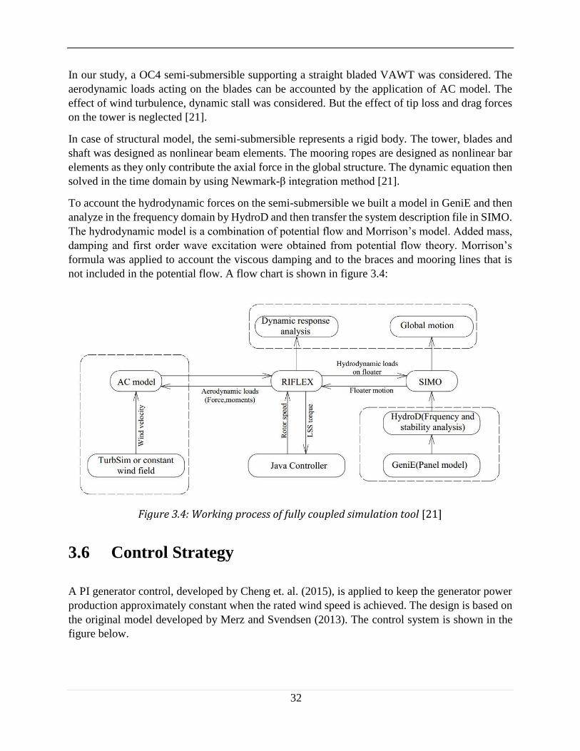
To account the hydrodynamic forces on the semi-submersible we built a model in GeniE and then
analyze in the frequency domain by HydroD and then transfer the system description file in SIMO.
The hydrodynamic model is a combination of potential flow and Morrison’s model. Added mass,
damping and first order wave excitation were obtained from potential flow theory. Morrison’s
formula was applied to account the viscous damping and to the braces and mooring lines that is
not included in the potential flow. A flow chart is shown in figure 3.4:
Figure 3.4: Working process of fully coupled simulation tool [21]
3.6 Control Strategy
A PI generator control, developed by Cheng et. al. (2015), is applied to keep the generator power
production approximately constant when the rated wind speed is achieved. The design is based on
the original model developed by Merz and Svendsen (2013). The control system is shown in the
figure below.

33
Figure 3.5: The generator control torque for a FVAWT [21]
Electric torque and generator power are measured and low pass filtered. The main aim is to reduce
the error between the measured and filtered rotational speed 𝛺𝑚𝑒𝑠 and reference rotational speed
𝛺𝑟𝑒𝑓. The reference rotational speed is measured as a function measured wind speed �� and low-
pass filtered electric torque ��. The updated electric torque is given by the following formula when
the quantity ∆𝛺 is fed through the proportional, integral and derivative path [21].
𝑇(𝑡) = 𝐾𝐺 (𝐾𝑃∆𝛺(𝑡) + 𝐾𝐼 ∫ ∆𝛺(𝜏)𝑑𝜏 + 𝐾𝐷
𝑡
0
𝑑
𝑑𝑡∆𝛺(𝑡)) (3.34)
In this equation, 𝐾𝐺 represents generator stiffness and 𝐾𝑃, 𝐾𝐼 and 𝐾𝐷 are the proportional, integral
and derivative gains respectively [21].
3.7 Load cases and environmental conditions
Several load cases were defined for this study to check the performance FVAWT. These cases are
used in the time domain simulation. We applied different wind speed and check the response of
the FVAWT. The data are shown in the tabulated form:
Table 3.1: Steady wind load cases for FVAWT
Load cases 𝑈𝑤[𝑚/𝑠] 𝐻𝑠[𝑚] 𝑇𝑝[𝑠] Wave condition Simulation length[𝑚] LC1.1 5 --- --- --- 3000
LC1.2 8 --- --- --- 3000
LC1.3 10 --- --- --- 3000
LC1.4 12 --- --- --- 3000
LC1.5 14 --- --- --- 3000
LC1.6 18 --- --- --- 3000
LC1.7 22 --- --- --- 3000
LC1.8 25 --- --- --- 3000

34
The potential theory model and the Morrison model then tested with turbulent wind and irregular
waves. We have different cases for waves. For each instance, we define different 𝐻𝑠 and 𝑇𝑝. The
different instances shown in tabular form:
Table 3.2: Load cases for turbulent wind and irregular waves
Load cases 𝑈𝑤
[𝑚/𝑠] 𝐻𝑠 [𝑚]
𝑇𝑝
[𝑠] 𝑇𝐼 [−]
Wave
condition
Simulation
length [𝑠]
LC2.1 5 2.10 9.74 0.224 Irregular 4600
LC2.2 8 2.55 9.86 0.174 Irregular 4600
LC2.3 10 2.88 9.98 0.157 Irregular 4600
LC2.4 12 3.24 10.12 0.146 Irregular 4600
LC2.5 14 3.62 10.29 0.138 Irregular 4600
LC2.6 18 4.44 10.66 0.127 Irregular 4600
LC2.7 22 5.32 11.06 0.121 Irregular 4600
LC2.8 25 6.02 11.38 0.117 Irregular 4600
Like steady wind cases, we consider eight different wind speed with rated speed 14 m/s. While for
steady wind test 𝐻𝑠 is very small but for irregular waves we need to consider this value. The total
simulation length was 4600s. But the last 1000s was taken into consideration. This is necessary
due to the transient effect on wind turbine.
To generate the turbulent wind, we use TrubSim software. It’s been developed to provide
numerical simulation of a full field flow that contains turbulent structures and reflect the proper
spatiotemporal turbulent velocity relationships[12]. Its purpose is to provide the wind turbine
designer with the ability to drive design code simulations. In our study, we use five different seeds
for each velocity. In total, we have 40 simulation result that we need to compare with old one as
well as measure the fluctuation of turbine output. But for simplicity we only consider one seed for
our discussion.
3.7.1 Environment
To design an offshore floating VAWT, we need to consider real environmental situation. First we
consider the steady wind condition and then considering wind and wave cases together. In some
places, it might necessary to consider the current, ice loads and other loading phenomenon. But
for simplicity we neglect this loads from our evaluation.
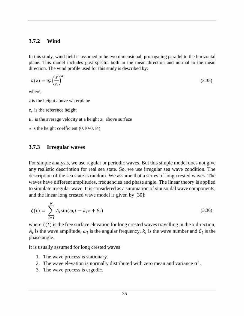
35
3.7.2 Wind
In this study, wind field is assumed to be two dimensional, propagating parallel to the horizontal
plane. This model includes gust spectra both in the mean direction and normal to the mean
direction. The wind profile used for this study is described by:
��(𝑧) = 𝑢𝑟 (𝑧
𝑧𝑟)𝛼
(3.35)
where,
z is the height above waterplane
𝑧𝑟 is the reference height
𝑢𝑟 is the average velocity at a height 𝑧𝑟 above surface
α is the height coefficient (0.10-0.14)
3.7.3 Irregular waves
For simple analysis, we use regular or periodic waves. But this simple model does not give
any realistic description for real sea state. So, we use irregular sea wave condition. The
description of the sea state is random. We assume that a series of long crested waves. The
waves have different amplitudes, frequencies and phase angle. The linear theory is applied
to simulate irregular wave. It is considered as a summation of sinusoidal wave components,
and the linear long crested wave model is given by [30]:
휁(𝑡) = ∑𝐴𝑖sin (𝜔𝑖𝑡 − 𝑘𝑖𝑥 + ℰ𝑖)
𝑁
𝑖=1
(3.36)
where 휁(𝑡) is the free surface elevation for long crested waves travelling in the x direction,
𝐴𝑖 is the wave amplitude, 𝜔𝑖 is the angular frequency, 𝑘𝑖 is the wave number and ℰ𝑖 is the
phase angle.
It is usually assumed for long crested waves:
1. The wave process is stationary.
2. The wave elevation is normally distributed with zero mean and variance σ2.
3. The wave process is ergodic.

36
Based on the assumption that the wave process follow Gaussian distribution the wave time
series is generated by Inverse Fast Fourier Transformation. The Joint Nordic Sea Wave
Project(JONSWAP) spectrum has been used for this study.
𝑆(𝜔) = 𝛼𝑔2
𝜔5exp (−𝛽 (
𝜔𝑝
𝜔)
4
) 𝛾
𝑒𝑥𝑝
(
−
(𝜔𝜔𝑝
−1)2
2𝜎2
)
(3.37)
𝛼 = 5.061𝐻𝑠
2
𝑇𝑝4(1 − 0.287ln (𝛾)) (3.38)
𝜎 = {0.07 𝑓𝑜𝑟 𝜔 < 𝜔𝑝
0.09 𝑓𝑜𝑟 𝜔 ≥ 𝜔𝑝 (3.39)
In equation 3.37, α is known as spectral parameter and γ is known as peaked parameter
which is in our case 3.3.
3.8 Decay test
Considering a mass-spring system, when a body is displaced from its mean position, the body
starts oscillating around the mean. But if we consider the damping of the system the amplitude
follows an exponential decay. In this study, we applied a force on the platform then release the
force. The body starts oscillating in the water. But the damping of water prevents this movement.
So, the amplitude decays as the time flows. If we observe the envelop of the amplitude curve, we
see the amplitude follows an exponential decay. The solution of the equation is given by the
following equation:
휂(𝑡) = 𝑒𝜉𝜔0𝑡𝑅 cos (𝜔𝑑𝑡 − 휃) (3.40)
where, 𝜔𝑑 = 𝜔0√1 − 𝜉2 and ξ is the damping ratio and 𝜔0 is the natural frequency. The term,
𝜔𝑑 is known as damping frequency.
For decay test, we applied ramp force and constant amplitude force for a certain amount of time.
Then the force was withdrawn and the decay measured. The simulation time varies 1300-1600s
for different degrees of freedom. The amplitude of the force also varies for different DOFs. Natural
period for six DOF between the new OC4 and the old OC4 model is shown below:

37
Table 3.3: Natural time period
Degrees of freedom Time Period for new OC4[s] Time Period for old OC4[s]
Surge 98.0 113.1460
Sway 97.3 113.1460
Heave 16.2 17.0440
Roll 25.8 20.6790
Pitch 25.4 20.6790
Yaw 72.1 80.4420
3.8.1 Discussion of results (Natural period)
The natural period depends on the mass of the platform, added mass related to the platform and
the stiffness of the platform. In the new design, we change several parameters as compared to the
old one. They are the dimension of the base column, dimension of the upper column, fairlead
position, total mass of the platform and center to center distance of the offset column. The mass
was reduced 3500 ton while the diameter of the upper and base column is decreased but the center
to center distance increased by two meters. Reducing the diameter of the upper column and base
column effectively reduces the water plane area of the platform that in turn reduces the total
stiffness of the platform. But increasing the center to center distance increase the stability and
stiffness of the platform.
Now as for surge, the fairlead position is changed but the length of the mooring line is same. This
reduces the overall stiffness of the mooring line. The mooring line is relatively flexible compared
to the old mooring line. In the surge direction, mooring line contributes the stiffness of the
platform. As the stiffness reduces so the natural period of surge.
As for heave, they are relatively same with a difference of 0.8s as compared to the old one. The
reason behind this decrease in period is that the diameter of the column decreases. This in turn,
reduces the stiffness in the vertical direction. Also, mass of the body contributes the overall
decrease of the natural heave period.
Figure 3.6: Time period for surge, heave, pitch and yaw

38
The same is true for the yaw motion. The natural period of the yaw depends on the water plane
area and mass of the body. In the new design, both reduces significantly. This might explain why
the natural period of yaw reduces as we compare the old one. But the natural period of pitch
increases 4.8s compared to the old one. This might happen due to the increasing distance between
two offset columns which increases the stiffness.
3.8.2 Damping ratio and the measurement technique
The ratio of two amplitudes at time step 𝑡𝑖 and 𝑡𝑖 + 𝑛𝑇𝑑 may be found from the measurement and
can be found from measurement and used to find the damping of a structure. The ratio can be
calculated from the following formula[5]:
𝑢𝑖
𝑢𝑖+𝑛=
𝑢(𝑡𝑖)
𝑢(𝑡𝑖 + 𝑛𝑇𝑑)=
𝑒𝜉𝜔0𝑡𝑖 𝑅 cos (𝜔𝑑𝑡𝑖−𝜃)
𝑒𝜉𝜔0(𝑡𝑖 +𝑛𝑡𝑑)𝑅 cos (𝜔𝑑(𝑡𝑖+𝑛𝑡𝑑)−𝜃)= 𝑒−𝜉𝜔0(𝑡𝑖 +𝑛𝑡𝑑) (3.41)
A measure of damping is to measure the damping for two amplitudes for a certain interval. The
logarithmic decrement can be defined as:
∧= ln [𝑢𝑖
𝑢𝑖+1] (3.42)
The connection between ∧ and ξ is expressed by setting n=1 in equation (2.10)
∧= ξ𝜔0𝑇𝑑 = 2𝜋𝜉
√1−𝜉2≈ 2πξ (As ξ is a very small quantity) (3.43)
So, the relation in equation (2.11) gives an approximate formula for damping ratio:
𝜉 ≈ 1
2𝜋𝑛ln [
𝑢𝑖
𝑢𝑖+𝑛] (3.44)
This is the final that we used for calculating damping ration in our study for six degrees of freedom.
The table and the figures were shown below:
Table 3.4: Damping ratio
Degrees of freedom Damping ratio for new OC4[s] Damping ratio for old OC4[s]
Surge 0.04471 0.04216
Sway 0.03738 0.03738
Heave 0.02303 0.02410
Roll 0.02827 0.02827
Pitch 0.02353 0.01718
Yaw 0.01145 0.01603

39
Figure 3.7: Damping ration for both platform
Figure 3.8: Time history of surge, heave, pitch and yaw (decay test)
3.8.3 Discussion of results (Damping ratio) The damping ration indicates the amount of damping in an oscillation. It’s the ration of the
damping of a system to the critical damping. Higher value indicates the damping is large and when
the value approaches one, there is no oscillation in the medium. The damping ration depends on
the mass and the stiffness of a system. If the damping ration is larger, the time period related to
the motion is also larger.
In our study, we can see the damping ratio for the old model is relatively larger. This is expected.
For the new OC4 semi-submersible we change different parameter such as water plane area,
distance, mass and others. As for surge motion, the damping ratio is relatively larger than other
motion. So, the time period for surge is also larger than any other case. This happened due to
40
change in stiffness of the mooring line. The mooring lines for the new one is less stiff than the old
one.
As for heave, the main contribution came from the base column and the water plane area. As the
diameter of the base column reduced this effectively change in damping ratio. For pitch and yaw
the damping ratio is larger for the old semi-submersible. This is mainly due to the reduction of
water plane area which effectively reduces the stiffness of the platform.
Now if we look at the figure for the decay test two parallel comparison is made for the two semi-
submersibles. It shows the time history of decay for different motion when no aerodynamic loads
are acting on the system. As we observe, in the beginning of the decay of OC4 semi-submersible
the decay was fast. The amplitude decays faster. This is due to the quadratic damping activated at
that time. Large amount of water displaced due to rapid movement. So, viscous damping is more
important. But as the time increases the amplitude decays slowly. This is due to the activation of
first order damping.

41
3.9 Results and discussions for steady wind test
3.9.1 Global motions
In the steady wind test, different wind loads are acting on the wind turbine. The wave forces are
zero by making the significant wave height very small. Then we run the analysis for 3000 s. The
first 2000 s is not taken into consideration. Only last 1000 s is considered. Transient effect need to
be consider. In order to reach a steady state, we need to wait for the first 2000 s.
At first we want to look at the motion characteristic of the FVAWT against wind speed. Here, the
four important degrees of freedom are surge, heave, pitch and yaw. The natural period of surge,
heave, pitch and yaw are 98.0s, 16.2s, 25.4s and 72.1s respectively. The tests are carried out in
calm water and the turbine is in the parked condition. The wind field is not present and hence
aerodynamic forces are not calculated.
Then we applied different steady wind load against VAWT and then noted the mean offset from
its original position. The mean offset data is shown below:
Table 3.5: Mean offset under different load cases
Wind speed
[𝑚/𝑠] Mean Surge
[𝑚] Mean Heave
[𝑚] Mean Pitch
[𝑑𝑒𝑔] Mean Yaw
[𝑑𝑒𝑔] 5 1.2062 -0.0211 0.4874 -0.2758
8 3.1407 -0.0236 1.2309 -0.6845
10 4.9877 -0.0281 1.9349 -1.0498
12 6.6165 -0.0336 2.5325 -1.6566
14 7.9087 -0.0391 2.9948 -2.3945
18 7.2262 -0.0363 2.7144 -2.7659
22 7.6625 -0.0382 2.8738 -2.7888
25 8.2941 -0.0412 3.1039 -2.8533
Figure 3.9: Mean offset vs wind speed (surge, heave, pitch and yaw)
-2
0
2
4
6
8
10
5 8 10 12 14 18 22 25
Dis
pla
cem
ent[
m]
Wind speed[m/s]
Wind speed vs mean displacement
Mean surge
Mean heave
-4
-3
-2
-1
0
1
2
3
4
5 8 10 12 14 18 22 25
Dis
pla
cem
ent[
deg
]
Wind speed[m/s]
Wind speed vs mean displacement
Mean pitch
Mean yaw
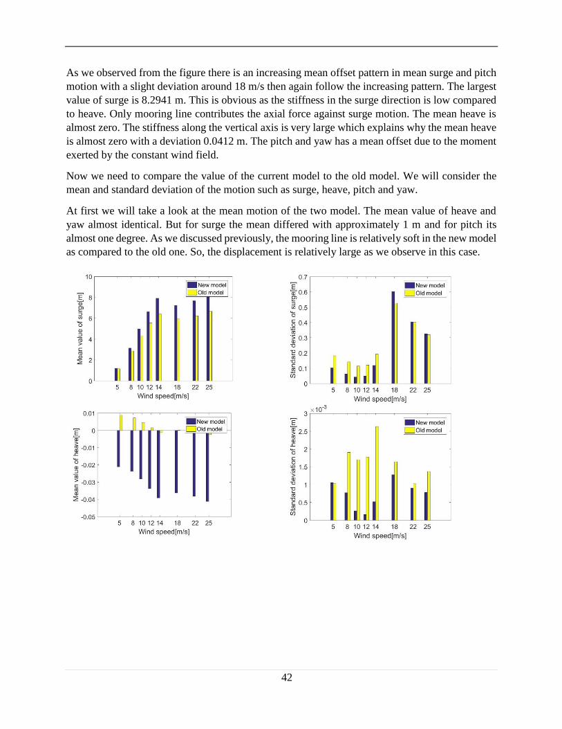
42
As we observed from the figure there is an increasing mean offset pattern in mean surge and pitch
motion with a slight deviation around 18 m/s then again follow the increasing pattern. The largest
value of surge is 8.2941 m. This is obvious as the stiffness in the surge direction is low compared
to heave. Only mooring line contributes the axial force against surge motion. The mean heave is
almost zero. The stiffness along the vertical axis is very large which explains why the mean heave
is almost zero with a deviation 0.0412 m. The pitch and yaw has a mean offset due to the moment
exerted by the constant wind field.
Now we need to compare the value of the current model to the old model. We will consider the
mean and standard deviation of the motion such as surge, heave, pitch and yaw.
At first we will take a look at the mean motion of the two model. The mean value of heave and
yaw almost identical. But for surge the mean differed with approximately 1 m and for pitch its
almost one degree. As we discussed previously, the mooring line is relatively soft in the new model
as compared to the old one. So, the displacement is relatively large as we observe in this case.

43
Figure 3.10: Mean offset and standard deviation of motions under different load cases
Now we will compare the standard deviation of the motion. As it is seen from the figure the
standard deviation is very small for these four motion. In case of heave and pitch they are very
small and for surge this value is 0.1 m and for yaw 0.18 degree approximately. One thing need to
be satisfied. In most cases, the first order excitation energy is in the range of 5-15 s. In order to get
rid from the resonance our platform natural period must be outside of this range. The only motion
that might cause this resonance problem is heave. But if we take the standard deviation of the
motion then we realize highest deviation from the mean of a motion component. The deviation of
heave is very small.
3.9.2 Turbine performance
Here we include four different parameters for comparison. The parameters are rotor speed,
generator power, aerodynamic thrust and aerodynamic torque. In this section, the figure in the left
gives the mean and in the right side gives the standard deviation of the parameter. The load cases
are equal in each case.

44
Figure 3.11: Mean and standard deviation of turbine performance (new FVAWT, old FVAWT and landbaed VAWT)
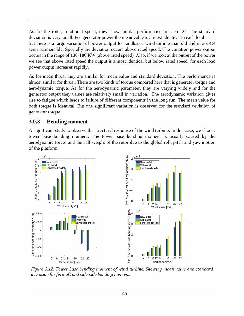
45
As for the rotor, rotational speed, they show similar performance in each LC. The standard
deviation is very small. For generator power the mean value is almost identical in each load cases
but there is a large variation of power output for landbased wind turbine than old and new OC4
semi-submersible. Specially the deviation occurs above rated speed. The variation power output
occurs in the range of 130-180 KW (above rated speed). Also, if we look at the output of the power
we see that above rated speed the output is almost identical but below rated speed, for each load
power output increases rapidly.
As for mean thrust they are similar for mean value and standard deviation. The performance is
almost similar for thrust. There are two kinds of torque compared here that is generator torque and
aerodynamic torque. As for the aerodynamic parameter, they are varying widely and for the
generator output they values are relatively small in variation. The aerodynamic variation gives
rise to fatigue which leads to failure of different components in the long run. The mean value for
both torque is identical. But one significant variation is observed for the standard deviation of
generator torque.
3.9.3 Bending moment
A significant study to observe the structural response of the wind turbine. In this case, we choose
tower base bending moment. The tower base bending moment is usually caused by the
aerodynamic forces and the self-weight of the rotor due to the global roll, pitch and yaw motion
of the platform.
Figure 3.12: Tower base bending moment of wind turbine. Showing mean value and standard deviation for fore-aft and side-side bending moment

46
When the wind started to flow from the front side of rotor then this side is known as fore side and
the opposite part is known as aft side. As wind flows from the front side of the rotor it creates a
large bending moment at the tower base which is known as tower base fore-aft bending moment.
Remaining side bending moment is known as side-side bending moment. It is obvious that the fore
aft bending moment is much larger than the side-side bending moment. It is also evident from the
figure of the fore-aft and side-side bending moment.
As for the fore-aft bending moment the largest value found from the new OC4 semi-submersible.
This can be explained in following way. The weight of the new OC4 semi-submersible is greatly
reduced. This increases the angular motion of the new semi-submersible because same load is
acting on the lighter platform. This increases the angular offset of the new platform compared to
the old platform. Extra increment of the angular offset compensated by the large fore-aft bending
moment. But for bottom fixed turbine there is no such motion. The standard deviation is very large
for the fore-aft bending moment. This might lead to fatigue of different component in the long run.
Standard deviation is always larger for landbased wind turbine.
As for side-side bending moment the largest bending moment found from landbased wind turbine.
Also, above rated speed the bending moment acting in the opposite direction. The standard
deviation is also large for side-side bending moment.
3.9.4 Mooring line tension
In this analysis, the mooring line is divided into two parts. One part is connected to the platform
and the other rest on the sea bed. Here we are comparing the first part. Tension which is acted on
the three-catenary mooring line is compared to the old model.
The axial force acting on the mooring line is almost similar for all load cases. But there is a
difference in the standard deviation of axial force acting on the mooring line. It’s obvious from the
above figure that the standard deviation for the older one is larger than the new one. The largest
force acting on the mooring line 2. This is expected as the BC-2 column is directed towards the
wave and wind direction. Also, the force in the mooring line 1 and 2 have same magnitude. This
happens due to the symmetry of the platform: So, the total forces distributed in the two mooring
lines.

47
Figure 3.13: Mean and standard deviation of axial force on mooring line 1, 2 and 3

48
3.10 Turbulent wind and irregular waves (Results and
discussion)
3.10.1 Global motion
For Darrieus FVAWTs, the mean deviation of platform motion was mainly due to the load exerted
by the wind field. This concept is applicable for straight bladed floating VAWT which is
considered in this study. Here we present the data comparison for seed 1. The highest mean value
of surge occurs at 25 m/s and the maximum value is 8 m. The mean value of pitch and yaw is 3.15
degrees and -2.87 degrees respectively. As for sway, heave and roll the deflection from its mean
value is small. As for this motion the stiffness and damping in the respective direction is very large.
As for surge, pitch and yaw the mean value of motion is increasing and the highest at 14 m/s and
the increasing rate is approximately constant or very small. Also, the deflection from the mean
value is larger than the previous OC4 model. The effect of mean value of motion for different load
cases is shown the following figure 3.14.
Figure 3.14(a): Mean offset of of different degrees of freedom

49
Figure 3.14(b): Mean offset of of different degrees of freedom
The standard deviation is highest for surge and yaw. As for surge motion highest deviation
occurred for surge at 12 m/s and the value of deviation is 1.733 m for new model and for old model
the maximum deviation occurs at 10 ms-1 wind velocity. As for yaw motion the maximum
deviation occurs for new and old model at rated speed and the deviation is 1.374 and 1.092 degrees
respectively. For other motions, the mean value is small so the standard deviation is also small.
The discrepency in between two platform is mainly due to the changing of different design
parameters.
Figure 3.15(a): Standard deviation of surge, sway

50
Figure 3.15(b): Standard deviation of heave, roll, pitch and yaw
Power spectral analysis is carried out for surge and yaw for load cases LC 1.3 and LC 1.7. The
main contribution of surge and yaw coming from the wind velocity. The figure is shown below:
Figure 3.16(a): Power spectra for surge at LC 2.3
Figure 3.13(b): Power spectra for surge at LC 2.7

51
Figure 3.16(c): Power spectra for yaw at LC 2.3
Figure 3.16(d): Power spectra for yaw at LC 2.7
The main contribution came from the wind velocity as shown by the large peak. The smaller peak
came from the wave contribution but there is another peak for surge at LC1.7. The main
contribution lies in 0.07-0.08 rad/s.
3.10.2 Turbine performance
In our study, we are interested to look at the performance parameters such as rotor speed, power,
thrust and torque. As for generator power above rated speed the power production is almost similar
for both model. The maximum power produced for the wind turbine occurs at 14 m/s and the power
available in the generator is 5.2 MW approximately for both model. As for rotor speed the
maximum speed found at 14 m/s and then speed decreases gradually. The mean value of thrust and
torque follows the same pattern. Above rated speed the value increases slowly compared to the
value below rated speed. The mean value of maximum thrust occurs at 25 m/s and the value is 533
KN. For both model the value of the parameters are very close.

52
Figure 3.17: Mean value of rotor speed, generator power, thrust and torque
As for rotor speed, the standard deviation is relatively small for both cases. As power in the
generator, the maximum deviation occurs at 14 m/s and the rated generator power is 1006.4 KW.
It’s a very large deviation from the mean value. This is expected due to the huge fluctuation occur
for vertical axis wind turbine. It increases the possibility to reduce the life span of different
component of wind turbine as it leads to the fatigue of the structure. As for thrust and torque the
result differs slightly.

53
Figure 3.18: Standard deviation of turbine performance
3.10.3 Mooring line tension
To secure the OC4 platform we need to moored the platform with three catenary mooring lines
spreading symmetrically through vertical axis [25]. The fairleads are located at the top of the base
column which 14 m below the sea water line. Mooring line is divided into two parts. One is
mooring part which is connected to the platform and the other one is anchor which rest on the
seabed. Each line is separated from the other by 120 degree. One line is directed to the positive x
axis and the other two lines are symmetrically distributed with respect to the x axis. Each line has
an unstretched length 835.5 m and an equivalent mass per unit length 113.35 kg/m [25].
Here we used linearized mooring model. It should be noted that the mooring arrangement in old
platform is opposite than the new model. The result is shown below:

54
Figure 3.19: Tension on mooring line 1, 2 and 3
The forces in the mooring line is almost similar but there exists deviation in the mooring line force.
The largest force acting on the mooring line 2 due to its heading in the opposite direction of the
wave and wind. So, the standard deviation is also large for the mooring line 2. As for the 1st and
the 3rd mooring line, the force acting on them are of the same magnitude. This is possible due to
the symmetry of the platform. So, when the wind and wave hits on the platform the forces are
distributed on both lines.
Power spectral analysis was carried out to understand the contribution from different forces. In our
cases, only two loads are acting here. They are wind loads and wave loads. The analysis is carried
out for wind speed 10 and 22 ms-1. The mooring line we consider here for power spectral analysis
is the mooring line 2. The figure is shown below:
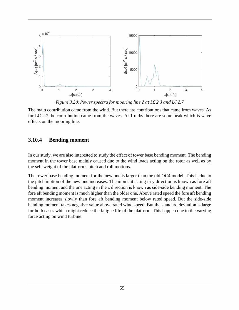
55
Figure 3.20: Power spectra for mooring line 2 at LC 2.3 and LC 2.7
The main contribution came from the wind. But there are contributions that came from waves. As
for LC 2.7 the contribution came from the waves. At 1 rad/s there are some peak which is wave
effects on the mooring line.
3.10.4 Bending moment
In our study, we are also interested to study the effect of tower base bending moment. The bending
moment in the tower base mainly caused due to the wind loads acting on the rotor as well as by
the self-weight of the platforms pitch and roll motions.
The tower base bending moment for the new one is larger than the old OC4 model. This is due to
the pitch motion of the new one increases. The moment acting in y direction is known as fore aft
bending moment and the one acting in the z direction is known as side-side bending moment. The
fore aft bending moment is much higher than the older one. Above rated speed the fore aft bending
moment increases slowly than fore aft bending moment below rated speed. But the side-side
bending moment takes negative value above rated wind speed. But the standard deviation is large
for both cases which might reduce the fatigue life of the platform. This happen due to the varying
force acting on wind turbine.

56
Figure 3.21: Tower base fore-aft bending moment
Figure 3.22: Tower base side-side bending moment
The spectral analysis is necessary to understand the contribution of different loads. As it is a three
bladed VAWT, 3P responses are prominent. The figure is shown below:

57
Figure 3.23: Tower base fore-aft bending moment for LC 2.3, LC 2.5 and LC 2.7
In between 0.3-1.2 rad/s, the response came from the wave response but the main contribution
came from the wind. Increasing the load, rises the peak significantly as it is evident from the figure.
3.11 Second order effect
So far we have discussed in this study based on the first order property of the wave. Now we want
to study the effect of second order on the performance of the new OC4 semi-submersible. Second
order effects cause on the loads or motions. There are three effects. They are as follows.
A mean value force (drift force)
A sum wave frequency oscillatory behavior (𝜔𝑖 − 𝜔𝑗)
A difference frequency oscillatory behavior (𝜔𝑖 + 𝜔𝑗)
For a sea state with S(ω), 𝜔𝑖, 𝜔𝑗 are the two regular wave components. Suppose two incident wave
components of a sea state with spectrum S(ω) and two waves with amplitude 휁𝑎1 and 휁𝑎2 and
frequency 𝜔1 and 𝜔2. The velocity potential is given by [31]
𝜙01(1)
=𝑔휁𝑎1
𝜔1𝑒𝑘1𝑧 cos(𝜔1𝑡 − 𝑘1𝑥 + 𝛼1) 𝜙02
(2)=
𝑔휁𝑎2
𝜔2𝑒𝑘2𝑧 cos (𝜔2𝑡 − 𝑘2𝑥 + 𝛼2) (3.45)
Velocity potential, is given by the following equation:
𝜙 = 𝜙1 + 𝜙2 = 𝜙1(1)(𝜔1) + 𝜙1
(2)(𝜔2) + 𝜙2(𝜔1, 𝜔2) (3.46)
Here 𝜙2(𝜔1, 𝜔2) is the combined effect of the incident waves. We analyze the features of the loads
associated with the contribution (𝜕𝜙1
𝜕𝑥)2 to the square velocity term at x=0.
𝜕𝜙1
𝜕𝑥= 𝐴1 cos(𝜔1𝑡 + 휀1) + 𝐴2cos (𝜔2𝑡 + 휀2)
(3.47)
(𝜕𝜙1
𝜕𝑥)
2
= 𝐴12𝑐𝑜𝑠2(𝜔1𝑡 + 휀1) + 𝐴2
2𝑐𝑜𝑠2(𝜔2𝑡 + 휀2) + 2𝐴1𝐴2(𝜔1𝑡 + 휀1)(𝜔2𝑡 + 휀2)

58
(𝜕𝜙1
𝜕𝑥)
2
=𝐴1
2 + 𝐴22
2+ 𝐴1
2 cos[2(𝜔1𝑡 + 휀1)]
2
+ 𝐴22 cos
[2(𝜔2𝑡 + 휀2)]
2+𝐴1𝐴2 cos(𝜔1 + 𝜔2) t + 휀1 + 휀2
+ 𝐴1𝐴2 cos(𝜔1 − 𝜔2) t + 휀1 − 휀2 So, the first term in the equation is a constant term which we are going to deal with. This is the
known as mean drift force [31].
3.12 Modelling in HydroD
First, the platform is modelled as a 3D panel model is GeniE. We define the mesh size in GeniE
1.2 m. Then export the FEM model in HydroD. Then we use frequency domain analysis to find
out the response of the body. We use second order drift force in our calculation. The wave heading
angle is selected from 0°-180° with an interval of 30°. Sixty frequency was chosen for the analysis
and total depth is 200 m. The SESAM interface file is then import in the SIMO to create a system
description file. The final model is then modified according to the description in chapter 2. They
are buoyancy compensation factor, design of slender element etc.
There are different technique available for estimating the drift force. Some of them are the direct
pressure integration and conservation of the fluid momentum. In our study, we use pressure
integration technique in which integration is carried out along the instantaneous wetted surface
area of the body [31].
𝐹 = ∫𝑝𝒏𝑑𝑠 = −𝜌 ∫ (𝜕𝜙
𝜕𝑡+
1
2|𝛻𝜙|2 + 𝑔𝑧)𝒏𝑑𝑠 = 0
𝑆𝐵
(3.48)
3.13 Newman approximation
Consider a sea state with wave spectrum 𝑆(𝜔). Then the amplitude is given by
𝐴𝑗 = √2𝑆(𝜔𝑗)∆𝜔 (3.49)
Now we extend the two waves expressing the second-order loads due to the sea state as
𝐹𝑖𝑆𝑉 = ∑ ∑ 𝐴𝑗
𝑁𝑘=1 𝐴𝑘
𝑁𝑗=1 [𝑇𝑗𝑘
𝑖𝑐 cos(𝜔𝑘 − 𝜔𝑗)𝑡 + (휀𝑘 − 휀𝑗) +𝑇𝑗𝑘𝑖𝑠 sim(𝜔𝑘 − 𝜔𝑗)𝑡 +
(휀𝑘 − 휀𝑗)] (3.50)
This equation includes both the mean and slow drift contributions. The second order transfer
functions in the equation is difficult to compute and very time consuming. Newman approximated
the equation in the following way. According to Newman we can simplify the equation with the
following assumption [31]:

59
𝑇𝑗𝑘𝑖𝑐 = 𝑇𝑘𝑗
𝑖𝑐 =1
2(𝑇𝑗𝑗
𝑖𝑐 + 𝑇𝑘𝑘𝑖𝑐 ) and 𝑇𝑗𝑘
𝑖𝑠 = −𝑇𝑘𝑗𝑖𝑠 (3.51)
It implies that the values of the second order transfer functions along the line 𝜔𝑗 = 𝜔𝑘. If we
observe the equation it satisfies when j=k. The approximation holds good if:
The second order transfer function is close to the line 𝜔𝑗 = 𝜔𝑘.
𝑇𝑗𝑘𝑖𝑐 and 𝑇𝑘𝑗
𝑖𝑐 do not change much with the frequency.
If both conditions hold true, then 𝑇𝑗𝑗𝑖𝑐 ≅ 𝑇𝑘𝑘
𝑖𝑐 and we have [31]
0.5(𝑇𝑗𝑗𝑖𝑐 + 𝑇𝑘𝑘
𝑖𝑐 ) ≅ √𝑇𝑗𝑗𝑖𝑐𝑇𝑘𝑘
𝑖𝑐 (3.52)
This means we can use geometric mean to approximate 𝑇𝑗𝑘𝑖𝑐 and 𝑇𝑘𝑗
𝑖𝑐. Introduing Newman
approximation along with geometric mean in the main expression gives:
𝐹𝑖𝑆𝑉 ≅ ∑ ∑ 𝐴𝑗
𝑁𝑘=1 𝐴𝑘√𝑇𝑗𝑗
𝑖𝑐𝑇𝑘𝑘𝑖𝑐𝑁
𝑗=1 cos(𝜔𝑘 − 𝜔𝑗)𝑡 + (휀𝑘 − 휀𝑗) (3.53)
The resulting solution depends only on the transfer function 𝑇𝑗𝑗𝑖𝑐 and 𝑇𝑘𝑘
𝑖𝑐 . They depend only on the
first order linear solution if there is no current and forward motion. So, per the Newman
approximation it’s no longer necessary to calculate the second order velocity potential 𝜙2. This in
turn significantly reduces the labor and the computational cost.
3.14 Results and discussion on the effect of mean drift
Prior to comparative study, A series of load tests was evaluated. Here we use turbulent and
irregular wave condition and observe the effect of mean drift force. We used eight different load
cases for wind and used seed 1 to generate the turbulent wind by using TurbSim. Then we perform
the simulation for 4600s and evaluate the value of last 1000s due to the transient effect of wind
turbine and compared the result with the first order effect. Same load cases are used for second
order effect as we used for turbulent and irregular waves. The results will be discussed in different
section.
3.14.1 Platform motion
Due to the difference in wave interaction in the platform the small variation in the results might be
expected. The figure shows the mean and standard deviation of the motion such as surge, heave,
pitch and yaw. The trend lines are very similar compared to the first order model. The trends in
the mean value of surge, heave are very similar though they differed by their amplitude. The reason
is that the mean offset is caused by the wind thrust force. As the stiffness in the heave direction is

60
larger the deviation is very small compared to surge motion. The sway and roll motions are caused
by the aerodynamic lateral loads acting on the rotor. The trend line is also similar in this case. The
main contribution of stiffness in the surge and sway direction is coming from the catenary mooring
line and for other motions, the water place area contributes the stiffness of the platform.
Figure 3.24: Mean offset of surge, pitch and
yaw(mean drfit) Figure 3.25: Standard deviation
of surge, pitch and yaw(mean drfit)
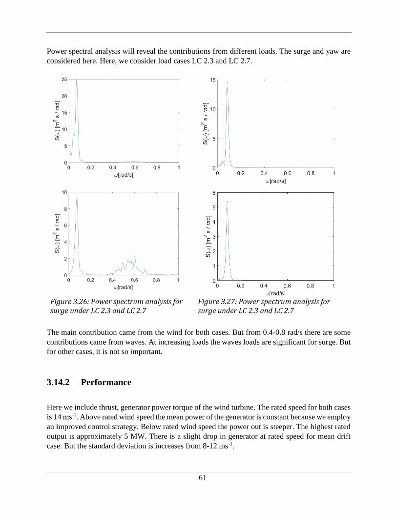
61
Power spectral analysis will reveal the contributions from different loads. The surge and yaw are
considered here. Here, we consider load cases LC 2.3 and LC 2.7.
Figure 3.26: Power spectrum analysis for surge under LC 2.3 and LC 2.7
Figure 3.27: Power spectrum analysis for surge under LC 2.3 and LC 2.7
The main contribution came from the wind for both cases. But from 0.4-0.8 rad/s there are some
contributions came from waves. At increasing loads the waves loads are significant for surge. But
for other cases, it is not so important.
3.14.2 Performance
Here we include thrust, generator power torque of the wind turbine. The rated speed for both cases
is 14 ms-1. Above rated wind speed the mean power of the generator is constant because we employ
an improved control strategy. Below rated wind speed the power out is steeper. The highest rated
output is approximately 5 MW. There is a slight drop in generator at rated speed for mean drift
case. But the standard deviation is increases from 8-12 ms-1.

62
Figure 3.28: Performance of wind turbine (mean drift)
The thrust and torque also follows the same pattern and characteristic response is similar. But there
is a discrepancy in the standard deviation due to the variation for mean drift force. But overall the
performance is similar.

63
3.14.3 Tower base bending and mooring line force
The figure shown below compares the result for mean value and standard deviation of tower base
bending moment and mooring line tension.

64
Figure 3.29: Mean value of mooring force on line 1, 2 and fore-aft, side-side bending moment acting on tower base (from up-down)(mean drift)
Figure 3.30: Standard deviation of mooring force on line 1, 2 and fore-aft, side-side bending moment acting on tower base (from up-down)(mean drift)
The mooring line tension for the second one is larger than the other mooring line as it was deployed
along the direction of wind and wave. The distribution in the first and the third mooring line is
almost same due to the symmetry of the platform. Also for the second mooring line the force is
increased 20-60 KN due to the wave wind misalignment. The standard deviation is affected than
the mean value because the mean value of mooring line forces are primarily determined by the
wind loads. But the standard deviation is affected by the frequency component interaction.
The mean and standard deviation of tower base bending moment for the platform for both cases
are similar without showing any abrupt changes. The contribution of different cases can be found
from the spectrum analysis. The main contributions came from the wind. As for the waves, they
increases their interaction as the load cases increases. The figure is shown below:

65
Figure 3.31: Power spectra for mooring line 2 (LC 2.3, LC 2.5 and LC 2.7)
Figure 3.32: Power spectra for tower base bending moment (LC 2.3, LC 2.5 and LC 2.7)
Waves loads effect is seen for mooring line from 0.3-1.5 rad/s and for bending moment the main
contribution of waves was in between 0.3-1.2 rad/s. The main response came from the wind loads
as seen from each figure which is indicated by the peak resonance near 2.8 rad/s.

66
Chapter 4
Conclusions and recommendation for future works
4.1 Conclusions
In this study, a FVAWT model was developed based on AC cylinder code originally developed by
Madsen and code was developed by Cheng. The code was then coupled with SIMO-RIFLEX, a
fully coupled simulation tool used for the time domain simulation for floating VAWT. Then the
new model is compared with old OC4 semi-submersible. Using fully coupled simulation tool the
performance of the system is carried out. In this thesis, we carried out the motion analysis,
performance analysis of the wind turbine, mooring line force and bending moment on the tower
base both for steady wind and the turbulent wind and irregular waves. This chapter will deal with
the main conclusions and recommendation for future work:
We developed this new OC4 semi-submersible based on the old OC4 semi-submersible.
So, we optimize the parameter and carried out detail calculation whether the platform
satisfied the stability criteria. To check the natural frequency and damping ratio we carried
out the decay test in SIMO-RIFLEX-AC without calculating any contribution from wind.
The result is quite satisfactory. The natural frequency for different motion is outside the
range of the first order excitation force. As we mentioned, in this study we reduce the
weight of the platform significantly so the stiffness and added mass of the platform
decreases which in turn effect the natural frequency of the platform. This was evident from
the comparison of both platform. The new model that was developed in this thesis, has
reduced natural frequency than the older one.
Then we carry our analysis for steady wind test. For steady wind test, we use AC method
to calculate the aerodynamic loads on the wind turbine. We used a series steady wind test
and check the performance. To improve the result, we used BL dynamic stall model. But
we neglect the tower shadow, tip loss in our study. This might affect the result a little bit.
We check motion of the platform, turbine performance, mooring line tension and bending
moment at the tower base. This time we compare three different model and check the
output of the result. The result for old OC4 and new OC4 is similar the result for landbased
wind turbine is varying in result. The standard deviation of power, torque and thrust varies

67
greatly. This is one of the disadvantages of wind turbine which trigger the fatigue of the
turbine component. But the fatigue of different component can be reduced by applying
composite materials. Also, by using improved control strategy we can limit the range of
torque and generator power output.
For turbulent wind and irregular waves there are eight different loading conditions for
wind speed and five different turbulent seeds for each loading conditions. We only study
on the effect of seed 1 and seed 5. For turbulent wind, we used TurbSim software. The
loading effect for wind and wave increases the response of the system. If we look at turbine
performance, we can easily verify this. As the loading condition changes the standard
deviation is also increased. The standard deviation on mooring line force increase
approximately twice than the steady wind condition. The fore-aft bending moment is
larger in the tower base. So, we need to employ different strategy to reduce the fore aft
bending moment. Otherwise the cyclic loading on the tower base reduce the fatigue life of
the wind turbine.
Finally, we are interested on the topic of second order effect on the system. There are three
different types of wave component interaction. They are sum frequency effect, difference
frequency effect and mean drift force. Here we only employ the mean drift effect.
4.2 Recommendation for future work
Here we only consider the normal operating conditions. The simulation in the parked and
fault conditions are also of interest.
The main disadvantages of VAWTs is the less efficiency and severe fatigue problem. To
make it sustainable in the long run one need to solve the problem. So, one interesting
analysis field is to improve the fatigue conditions of the VAWTs.
Here we consider three different VAWT models. All of them are straight bladed VAWTs.
There are different interesting blade configuration for VAWTs. One can carry out the study
for other rotor type such as helical bladed rotor, Savonius rotor etc.
A Pi generator controller is employed in this study. An improved control strategy could be
designed to maintain the constant power by reducing the rotational speed of the rotor at
high wind speed.
Drift force is the only second order effect that we study here. But one can also extend the
study and investigate the slowly varying drift force and sum frequency effect on the total
system.
Here we only look at the OC4 floater for VAWT. But a comparison on FHAWT and
FVAWT will further reveals the advantages and disadvantages of the two model. Also,
OC4 FVAWT concept need to compare with other floater such as TLP, Spar. Moreover,
the investigation might expand for H-type, V-type and helical-bladed rotor.
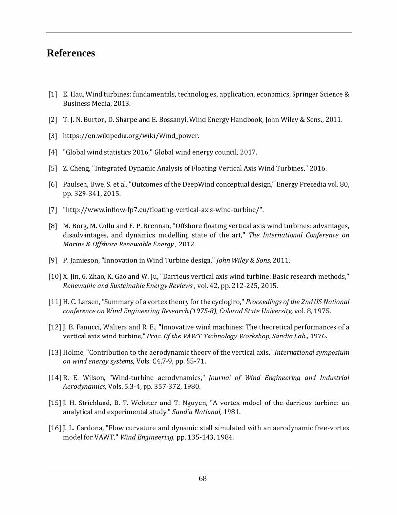
68
References
[1] E. Hau, Wind turbines: fundamentals, technologies, application, economics, Springer Science &
Business Media, 2013.
[2] T. J. N. Burton, D. Sharpe and E. Bossanyi, Wind Energy Handbook, John Wiley & Sons., 2011.
[3] https://en.wikipedia.org/wiki/Wind_power.
[4] "Global wind statistics 2016," Global wind energy council, 2017.
[5] Z. Cheng, "Integrated Dynamic Analysis of Floating Vertical Axis Wind Turbines," 2016.
[6] Paulsen, Uwe. S. et al. "Outcomes of the DeepWind conceptual design," Energy Precedia vol. 80,
pp. 329-341, 2015.
[7] "http://www.inflow-fp7.eu/floating-vertical-axis-wind-turbine/".
[8] M. Borg, M. Collu and F. P. Brennan, "Offshore floating vertical axis wind turbines: advantages,
disadvantages, and dynamics modelling state of the art," The International Conference on
Marine & Offshore Renewable Energy , 2012.
[9] P. Jamieson, "Innovation in Wind Turbine design," John Wiley & Sons, 2011.
[10] X. Jin, G. Zhao, K. Gao and W. Ju, "Darrieus vertical axis wind turbine: Basic research methods,"
Renewable and Sustainable Energy Reviews , vol. 42, pp. 212-225, 2015.
[11] H. C. Larsen, "Summary of a vortex theory for the cyclogiro," Proceedings of the 2nd US National
conference on Wind Engineering Research.(1975-8), Colorad State University, vol. 8, 1975.
[12] J. B. Fanucci, Walters and R. E., "Innovative wind machines: The theoretical performances of a
vertical axis wind turbine," Proc. Of the VAWT Technology Workshop, Sandia Lab., 1976.
[13] Holme, "Contribution to the aerodynamic theory of the vertical axis," International symposium
on wind energy systems, Vols. C4,7-9, pp. 55-71.
[14] R. E. Wilson, "Wind-turbine aerodynamics," Journal of Wind Engineering and Industrial
Aerodynamics, Vols. 5.3-4, pp. 357-372, 1980.
[15] J. H. Strickland, B. T. Webster and T. Nguyen, "A vortex mdoel of the darrieus turbine: an
analytical and experimental study," Sandia National, 1981.
[16] J. L. Cardona, "Flow curvature and dynamic stall simulated with an aerodynamic free-vortex
model for VAWT," Wind Engineering, pp. 135-143, 1984.

69
[17] H. A. Madsen, The Actuator Cylinder: A flow model for Vertical Axis Wind Turbine, Institute of Industrial Constructions and Energy Technology, Aalborg University Centre, 1982.
[18] I. Paraschiviou, Wind turbine design: emphasis on the darrieus concept, 1 ed., Montreal:
Polytechnic International Press, 2001.
[19] J. H. Strickland, B. T. Webster and T. Nguyen, "Vortex model of the darrieus turbine: an
analytical and experimental study," American Society of Mechanical Engineers, 1979.
[20] K. Dixon, "The near wake structure of a vertical axiswind turbine (Master's thesis)," TU Delft,
Netherlands, 2009.
[21] Z. Cheng, H. A. Madsen, Z. Gao and T. Moan, "A fully coupled method for numerical modeling
and dynamic analysis of floating vertical axis wind turbines," Renewable Energy, vol. 107, pp.
604-619, 2017.
[22] L. TJ and H. AM., How 2 HAWC2, the user’s manual, Risø National Laboratory, Technical
University of Denmark, 2013.
[23] D. N. Veritas, DNV-OS-J103: Design of Floating Wind Turbine Structures., 2013.
[24] Z. Cheng, H. A. Madsen, Z. Gao and T. Moan, "Aerodynamic modeling of floating vertical axis
wind turbines using the actuator cylinder flow method," ScienceDirect, vol. 94, pp. 531-543,
2016.
[25] A. Robertson, J. Jonkman, M. Masciola and e. al, "Definition of the semisubmersible floating
system for phase II of OC4. No. NREL/TP-5000-60601," National Renewable Energy Laboratory
(NREL), Golden, CO.,, 2014.
[26] H. Aagard Madsen, T. J. Larsen, U. Schimdt Paulsen and L. Vita, "Implementation of the Actuator
Cylinder Flow Model in the HAWC2 code for Aeroelastic Simulations on Vertical Axis Wind
Turbines," DTU orbit, p. 12, 2013.
[27] C. M. Larsen, Marine Dynamics, Trondheim: Department of Marine Technology, NTNU, 2015.
[28] M. Greco, Lecture notes on Sea loads, 2012.
[29] P. J. Moriarty and A. C. Hansen, "AeroDyn theory manual," National Renewable Energy Lab.,
Golden, CO (US), 2005.
[30] O. Faltinsen, Sea Loads on Ships and Offshore Structures, vol. 1, Cambridge University Press,
UK, 1993.
[31] B. J. Jonkman, "TurbSim user's guide: Version 1.50," 2009.
[32] L. Vita, T. Friis Pedersen and H. Aagaard Madsen, "Offshore Vertical Axis Wind Turbine with
Floating and Rotating Foundation," Technical University of Denmark, 2011.
70
[33] Z. Cheng, H. A. Madsen, Z. Gao and T. Moan, "Effect of number of blades on the dynamics of floating straight-bladed vertical axis wind turbines," Renewable Energy, vol. 101, pp. 1285-
1298, 2017.
[34] J. Wayne, Rotorcraft Aeromechanics, vol. 36, Cambridge university press, 2013.
[35] M. Leimeister, Rational Upscaling and Modelling of a Semi Submersible Floating Offshore Wind
Turbine, Trondheim: NTNU, TU Delft, 2016.