Original Research

______________________________________________________________________________

Design and Advantages of a Bioretention Area as a Best Management Practice for Low Impact

Development on The University of Texas at San Antonio

Felipe Alejandro Flores

Supervising Committee: Heather Shipley, Ph.D., Chair; Manuel Diaz, Ph.D.; Marcio Giacomoni,

Ph.D

May 02, 2016

__________________________________________________________________________

ABSTRACT Rainfall on urban areas causes polluted runoff water to contaminate the ground. A bioretention basin

can minimize this problem. In this project a bioretention basin was designed for future precipitation

changes regarding climate change. The bioretention basin was designed for new development on The

University of Texas at San Antonio Main campus and includes an economic analysis comparing three

different scenarios regarding media and materials. The basin includes sand and crushed glass as

media and Cedar Elm and Muhly grass plants as flora, which are native to San Antonio, to achieve

the pollution removal needed. After calculating the drainage area and future average precipitation, the

TSS removal required by the BMP was obtained. The equivalent depth, water quality volume treated,

and the footprint area were then calculated. Recycled water from a current building at UTSA was

tested and was suitable for irrigation. The results were as expected regarding the future average

precipitation and the size of the basin.

KEY WORDS: Environmental Engineering

2

INTRODUCTION

The construction of the built environment (e.g.

roads, buildings) affects natural ecosystem

processes and results in negative impacts to the

environment. Some examples of negative

impacts are seen during rainfall events when

runoff creates floods that are generated by

impervious areas causing polluted water to stay

on top of the developed area instead of

percolating into the ground. These problems can

be mitigated when making use of stormwater

management strategies such as Low Impact

Development (LID) (Dorman, et. al., 2013). LID

strategies are structural stormwater Best

Management Practices (BMPs) and planning

techniques intended to reproduce

predevelopment hydrologic conditions. An

example of a LID is a bioretention basin, which

channels water during a storm event to reduce

flooding and filters water to clean it from

pollutants carried from developed areas such as

parking lots (Dorman, et. al., 2013).

Bioretention is a common LID practice

because it mimics hydrologic conditions and

enhances biodiversity and water quality. In areas

such as Bexar County, it is important to

implement BMPs located on the Edward’s

Aquifer such as The University of Texas at San

Antonio (UTSA) to avoid polluted water to

percolate into the ground and pollute the aquifer.

The university can take advantage of the use of a

bioretention basin as a LID strategy to clean

polluted water, reduce flooding, and comply

with the Edward’s Aquifer regulations (Center

for Research, 2011). Currently, the university

has several sand filters built, but this project

focuses on the design of a bioretention basin,

which as an advantage uses vegetation to clean

pollutants, in an area where new buildings are

proposed to diminish the impact of increased

impervious areas. LIDs can easily be integrated

into existing development and built into new

development (Dorman, et. al., 2013). In order to

effectively select a BMP for a specific area, its

characteristics and features should be

understood; in addition, the design process must

be planned and followed in order to accurately

meet all the BMP objectives.

The design of a bioretention basin on UTSA

main campus is addressed in this project. This

basin was designed to be incorporated into new

development on campus to help with problems

related to the lack of natural systems by

reproducing predevelopment hydrologic

conditions. This project is important because it

deals with conditions that could become major

issues such as an increase in rainfall intensities

due to climate change and pollution of the

environment by contaminated water runoff from

future buildings to be built on campus (Dorman,

et. al., 2013). To fulfill the goal of this project,

the design includes research on climate change

in recent years to address intensity concerns.

There are four objectives addressed in this

project which are: 1) the calculation of the

treatment volume and equivalent depth of the

basin, 2) the footprint area of the proposed

development, 3) the selection of the basin’s

media and flora, and 4) conducting an economic

analysis of the different basin designs.

LITERATURE REVIEW

Stormwater Management Strategies

Rainfall over developed areas carries

pollutants to the ground by surface runoff, which

can become a problem. Therefore, stormwater

management strategies are needed to address

this problem and to reduce the peak runoff rates

and runoff volumes of storms (Center for

Research, 2011). There are several BMPs such

as bioretention areas, sand filters, bioswales,

green roofs, etc. used to convey, infiltrate, and

treat stormwater runoff, which differ in

effectiveness regarding the climate and area in

which they are built. These low impact

developments (LID) have different maintenance

cost and overall cost, which need to be

compared to design the most efficient one. In

addition, the drainage area that the LID will

receive is an important characteristic that needs

to be considered when choosing an LID since

they have different drainage area limits. For

example if the LID’s drainage area limit is

smaller than the drainage area it will receive,

then a combination of LIDs is needed to achieve

effective results. All BMPs have drainage area

3

limits but more than one system can be used in

parallel to cover all the drainage area necessary

(Center for Research, 2011).

Complying with the Regulations of the

Edward’s Aquifer

BMPs are required when building over the

Edward’s Aquifer region (Barrett, 2005). The

Edward’s Aquifer recharge zone is an area of

about 1500 square miles that includes part of

Bexar County (City Council of San Antonio,

1994). In this area, vertical faults occur exposing

fractured Edward’s limestone at the land surface.

The aquifer receives water from the flow

crossing the drainage area and from water that

percolates from major streams in the region. The

University of Texas at San Antonio is located

over the recharge zone of the Edward’s Aquifer.

The Edward’s Aquifer is unique in its ability to

recharge large quantities of water quickly, and

most of the water comes from infiltration of

rainwater that falls over the recharge zone

(Barrett, 2005). Consequently, the city of San

Antonio has passed a resolution for protection of

the aquifer that is enforced as high priority for

construction on the recharge zone.

The Edwards Aquifer Rules regulate the

activities that could potentially pollute the

waters associated with the aquifer and they

apply to recharge zones in Bexar County

(Barrett, 2005). The use of permanent BMPs is

required on areas over the aquifer to prevent

pollution caused by contaminated stormwater

runoff from the site. One of the requirements

established by the aquifer’s regulations is that at

least an 80% reduction of TSS (total suspended

solids) on runoff water needs to be achieved by

the BMPs in constructions over the aquifer

(Texas Commission on Environmental Quality,

2008). Studies indicate that bioretention basins

and sand filters as BMPs remove TSS by 89% in

average, which comply with the aquifer’s rules

(Dorman, et. al., 2013).

Sand Filter and Bioretention Basin Design

Sand filters and bioretention basins are two

stormwater management strategies that are used

to minimize problems related to water runoff.

Sand filters are basins that capture and filter

stormwater runoff by using a layer of sand and

they generally have a high rate removal for

phosphorus, BOD, zinc, copper, lead, nitrogen,

and fecal coliform. Sand filters consist of a bed

of sand that removes sediments and pollutants.

In these filters, bacteria slime is formed and

helps remove nutrients, organics, and coliform

bacteria from the water. Additionally, sand

filters can adapt to thin soils, limited-space

areas, and dry areas. Sand filters do not include

flora in its design (Barrett, 2005).

Bioretention basins use adsorption, plant

uptake, microbial activity, filtration, and

sedimentation to remove pollutants, and provide

high removal of sediment, metals, and organic

material (Dorman et. al., 2013). Bioretention

basins consist of a pretreatment system, a

surface ponding area, a mulch layer, and a

planted soil media; Figure 1 shows a schematic

diagram of a bioretention system. The vegetation

that needs to be included in the surface of the

basin is generally a combination of small to

medium-sized trees, shrubs, and groundcover.

The flora can adapt to size constraints and take

advantage of the semi-arid climate for

evapotranspiration in the San Antonio area

(Barrett, 2005). In addition, several physical,

biological, and chemical processes are applied in

a bioretention area to effectively remove

pollutants (United States Environmental

Protection Agency, 2015).

Figure 1. Schematic Diagram of a Bioretention

System.

4

The design of a LID, including bioretention

basins and sand filters, includes the following

steps. The size of the basin is first determined

followed by the selection of media required to

achieve the performance necessary. There are

different approaches to determine the water

quality volume and the method discussed here

follows the rational method (Dorman, et. al.,

2013). The volume-based method depends on

the runoff coefficients regarding the hydrologic

soil group. It was also developed to achieve total

suspended solids reduction targets regarding

annual rainfall volume. For this method, rainfall

depth is needed to get the volume necessary to

meet the treatment goals. Additionally,

hydrologic evaluations graphs are used to define

rainfall depth that must be treated to meet the

desired pollutant reduction goals (Dorman, et.

al., 2013). On the other hand, flow based design

methods are usually used for configuring inlets,

sizing, conveyance, or settling hydraulic control

(Dorman, et. al., 2013).

Bioretention Basin Advantages

Some of the advantages of a bioretention basin

include the removal of suspended solids, metals,

pollutants, nitrogen, phosphorus, and pathogens

from the water. They also reduce the peak runoff

rates for storms, reduce runoff volumes, and can

potentially recharge ground-water after filtering

it from pollutants (Dorman, et. al., 2013). In

addition, they are flexible to adapt to urban

retrofits and can be used in recharge zones,

karst, clays, and hotspots. Another important

characteristic of these basins is that they are well

suited for small areas and if multiple distributed

units are constructed, they can provide treatment

in large areas (Dorman, et. al., 2013).

Bioretention basins also enhance aesthetics and

provide habitat for different species. In addition,

in a bioretention basin the standing water is only

present for 12-24 hours, minimizing vector

control concerns (Dorman, et. al., 2013).

Research has shown that removal of TSS,

phosphorus, nitrogen, and fecal coliform is more

successfully achieved when vegetation is

included in a BMP such as in a bioretention

basin. Bioretention systems typically achieve a

TSS reduction of 89% efficiency (Center for

Research, 2011 and Dorman, et. al., 2013).

Likewise, pollutant removal is more achievable

when BMPs include media and robust

vegetation rather than just sand or a single plant

species (United States Environmental Protection

Agency, 2015). With the construction of a

bioretention basin, the UTSA main campus

could become more sustainable. Additionally, a

bioretention basin can be incorporated into a

development easily and its vegetation provides

shade, wind breaks, and absorbs noise (Center

for Research, 2011 and Dorman, et. al., 2013).

Besides its aesthetic benefits and its flexible

design, its implementation at UTSA can also

benefit it economically.

Additional benefits include the gaining of

credits for the Leadership in Energy and

Environmental Design (LEED) certification.

LEED credits are divided into sections and a

bioretention basin could earn credits in the

Sustainable Sites and Water Efficiency sections.

First of all, a bioretention basin could help the

new project earn up to three credits of Rainwater

Management subsection. Also, for the Heat

Island Reduction subsection it could earn up to

two credits by providing shade to nearby

developments with the flora planted. For the

Water Efficiency section, the BMP can earn up

to two credits in the Outdoor Water Use

Reduction section (USGBC, 2016). Since the

flora used in the basin will be native of the area,

not much water is going to be needed; the water

that will be needed is going to be obtained from

the recycled AC condensate water from the new

building developments on UTSA, as further

explained in section 3.3.

Economic Benefits of a Bioretention System

Municipalities usually encourage developers to

incorporate LID by offering incentives for

planned and existing developments (United

States Environmental Protection Agency, 2015).

The four most common categories of local

incentives are fee reductions, development

inducements, best management practices

installation subsidies, and awards and

recognition programs. Also, municipalities often

charge stormwater fees depending on the

impervious surface area on a property, but when

a LID system is used to reduce the amount of

runoff and clean for pollutants, the federal

5

government can help with the payments of this

fee (United States Environmental Protection

Agency, 2015). Likewise, incentives could be

available for developments using only LID

practices. This may incorporate propositions to

waive or decrease permit fees, accelerate the

permit procedure, or allow for higher density

developments. Furthermore, communities could

offer programs that subsidize the cost of the

materials that are used to construct the

bioretention system. Recognition programs are

held by the community to encourage LID

innovation. For example, the university could be

featured in articles, websites, and utility bill

mailings about their implementation of LIDs

increasing its prestige (United States

Environmental Protection Agency, 2015).

The city of San Antonio has implemented a

comprehensive plan for improving the

sustainability of the city by 2020. The SA2020

is a nonprofit organization to allow San Antonio

citizens to work with the city government to

achieve mutual goals. Moreover, the SA2020

program’s financial support for green

infrastructure such as LIDs comes from private

rather than public funding (Economides, 2014).

The San Antonio River Authority is also

promoting the construction of LID systems as

green infrastructure with several initiatives. To

name one, the Mission Verde Sustainability Plan

is investing in energy saving initiatives that

innovate and encourage green engineering such

as the LID systems (Office of Mayor Phil

Hardberger, 2009). Furthermore, San Antonio

has existing government and non-profit

programs each year to implement a green

infrastructure plan such as a bioretention basin.

The city of San Antonio Office of Sustainability

will also integrate green infrastructure in the

future, saving costs for developers and the city

in forthcoming construction of LIDs

(Economides, 2014).

LID approaches can be easily integrated into

capital improvement programs. One of the city’s

initiatives that indirectly support stormwater

management is the Tree Challenge Program

through the Parks and Recreation Department

(Economides, 2014). This program aims to

expand the tree canopy in San Antonio to

increase stormwater infiltration rates and reduce

the urban heat island effect. Through this

program, the city offers energy tax rebates when

planting trees on a property (Economides, 2014).

Although the program takes stormwater

management as a secondary benefit, it directly

recognizes the value of tree canopy. The design

of a bioretention basin at UTSA includes

vegetation and media that could be registered in

the Tree Challenge Program for CPS energy tax

rebates.

LID and green infrastructures result in

multiple financial, environmental, and social

benefits. Financial case studies for LID

implementations were made for Milwaukee,

Portland, Philadelphia, and the Sun Valley

watershed of Los Angeles County, which

monetized benefits using non-market economic

valuation techniques (U.S. Environmental

Protection Agency, 2013). In these benefit-cost

analyses, it was discovered that public benefits

of an LID, such as a bioretention basin, include

management cost, habitat creation, improved air

quality, and reduced carbon emissions. On the

other hand, private benefits include stormwater

volume reduction, reduced energy demand for

heating and cooling, and less stormwater facility

costs (U.S. Environmental Protection Agency,

2013). In another analysis, it was demonstrated

that for an equal investment amount and similar

overflow volume reductions, LIDs would

provide 20 times more benefit than traditional

stormwater infrastructure such as stormwater

pipes (U.S. Environmental Protection Agency,

2013). A bioretention basin will additionally

increase community aesthetics, increase wildlife

habitat, reduce heat island effect, and create a

possible reuse of the water for different activities

that will also benefit UTSA directly.

METHODS

To achieve the goal of designing a bioretention

basin for future building developments in UTSA

Main campus, the project has been broken-up

into four objectives. This chapter discusses the

methods that were used to carry-out these

objectives. The objectives are: 1) determine the

treatment volume and the equivalent depth of

6

water stored following design formulas, 2)

obtain the footprint area of the basin, 3) select

the media and flora, and 4) conduct economic

analysis on the proposed basins. For the fourth

objective, three bioretention basins were

designed with different media and materials to

select the most productive and the most

economical design. Climate change has been an

important factor for variations in rainfall depth

for the last few years and this factor is taken into

account in the design of the bioretention basin.

Determining the Contributing Drainage Area

The contributing drainage area is one of the

fundamental values needed to design a

bioretention basin. It defines the portion of the

site in acres that is contributing runoff to the

BMP. This area is utilized to determine the

water quality volume. The contributing runoff

was obtained based on the drainage contours of

the Texas Natural Resources Information

System (TNRIS) using Google Earth. First, from

the TNRIS webpage, the 2010 TNRIS 5ft

Contours Elevation GIS data was downloaded

along with the StratMap Elevation Contours.

The first represents the green contour lines and

the second one the red contour lines in Figure 2.

These contours were imported with a 2013

Bexar Metro 911 Image in ArcMaps version 10.

The 2 contours give different approaches to the

elevation of the terrain and they both specify

where the lowest point in the section is going to

be and thus, where the LID is going to be

located to receive all the runoff. In Figure 2, the

future development location is enclosed by the

black box and the basin’s location and lowest

point in the terrain is where the blue circle is.

After determining where the water is going to

flow, the contributing drainage area was

obtained using the Google measuring function.

Figure 2. Contour Lines and Bioretention Basin

Location.

Determining the Treatment Volume The proposed development for which the

bioretention basin is designed at The UTSA

Main campus will cover an area of 7.15 acres,

which will be the contributing drainage area for

the basin. Figure 3 shows UTSA Main campus

with some of the current sand filters marked by a

star and the proposed development area for

which the basin was designed is circled. The

proposed development will be near roads,

buildings, and parking lots; but the bioretention

basin will only receive runoff from the proposed

buildings due to the drainage already installed.

Consequently, for this project, the basin was

designed to handle the runoff received only from

the new development. The drainage area limit

for a bioretention basin is 10 acres and this

project’s drainage area falls inside the

parameters (Barrett, 2005). The volume-based

method was used to design the basin since it

uses annual rainfall precipitation to obtain the

water quality volume providing an easier way to

determine the volume based on precipitation

increases due to climate change (Barrett, 2005).

7

Figure 3. The University of Texas at San

Antonio Main campus from Google Earth.

The bioretention basin was designed to

account for future variations in climate. Climate

change has proven to increase average

precipitation throughout the years and so

projections were done to account for the increase

in precipitation (Downscaled CMIP3 and

CMIP5 Projections). The projections showed an

increase in future average annual precipitation

due to climate change and the basin was

designed to be able to function under future

precipitation increases. The projections were

downloaded from the Lawrence Livermore

National Laboratory archive. The data from this

archive is based on global climate projections

from the World Climate Research Programme’s

(WCRP’s) Coupled Model Intercomparison

Project Phase 3 (CMIP3). First, downscaled

CMIP3 daily climate and hydrology projections

developed using bias-correction and constructed

analogs (BCCA) were downloaded for the

specific area in which the project is located.

Daily climate and precipitation data for years

1961-2000, 2046-2065, and 2081-2099 was

obtained.

There were several different historical

projections used to obtain the precipitation

average for the future and included the possible

alterations due to climate change. The historical

projections obtained included five historical

projections from years 1961 to 2000, three

variable projections including years 2046 to

2065, and three future projections from years

2081 to 2099. After downloading them into an

Excel file, the yearly average was obtained for

each year and then the total average was

obtained for each projection. After that, graphs

were plotted for each projection showing an

increase of the precipitation average throughout

the years (section 4.1). In the design formulas

for the bioretention basin the yearly average

precipitation in inches was required so the

values were converted into in/yr.

To calculate the water quality volume of the

basin, the required TSS removal was obtained

using equation 3-1 followed by the load

removed by the bioretention basin as shown in

equation 3-2. For the required TSS removal

calculations, it was assumed that the appropriate

runoff coefficient of impervious areas is 0.9 and

0.03 for natural areas (Barrett, 2005). The new

development on campus is of 7.15 acres, which

include pervious and impervious areas that were

measured specifically for the calculations. The

TSS concentration increases to 170 mg/L in an

impervious area, and this is what was used for

the design. In addition, it was assumed that the

bioretention basin achieves an 89% of TSS

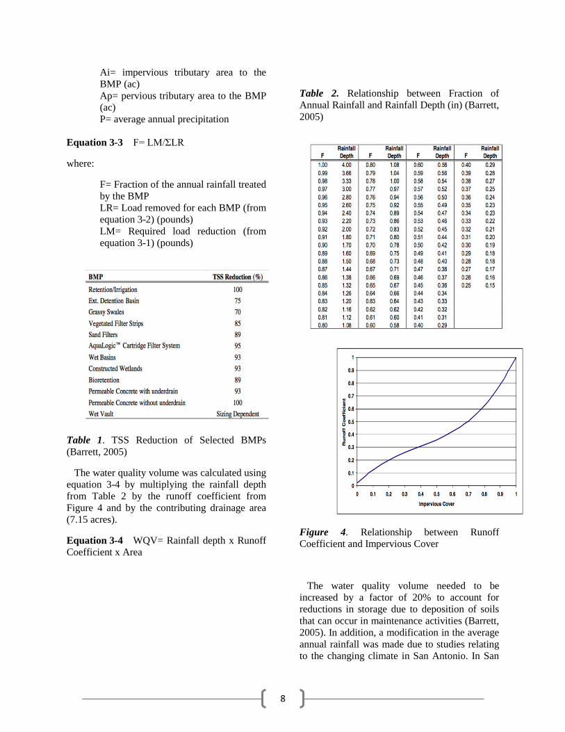
reduction according to Table 1 (Barrett, 2005).

The rainfall depth was obtained using equation

3-3, which is the fraction of annual rainfall

treated by the best management practice that

also determines if the BMP selected was good

enough for the treated area, and table 2 (Barrett,

2005).

Equation 3-1 LM= 27.2 (AN x P)

where:

LM= Required TSS removal (pounds)

AN= Net increase in impervious area

(acres)

P= Average annual precipitation

(inches)

Equation 3-2 LR= (BMP efficiency) x P x (Ai

x 34.6 + Ap x 0.54)

where:

LR= Load removed by BMP

BMP efficiency= TSS removal

efficiency (from table 1)

8

Ai= impervious tributary area to the

BMP (ac)

Ap= pervious tributary area to the BMP

(ac)

P= average annual precipitation

Equation 3-3 F= LM/ΣLR

where:

F= Fraction of the annual rainfall treated

by the BMP

LR= Load removed for each BMP (from

equation 3-2) (pounds)

LM= Required load reduction (from

equation 3-1) (pounds)

Table 1. TSS Reduction of Selected BMPs

(Barrett, 2005)

The water quality volume was calculated using

equation 3-4 by multiplying the rainfall depth

from Table 2 by the runoff coefficient from

Figure 4 and by the contributing drainage area

(7.15 acres).

Equation 3-4 WQV= Rainfall depth x Runoff

Coefficient x Area

Table 2. Relationship between Fraction of

Annual Rainfall and Rainfall Depth (in) (Barrett,

2005)

Figure 4. Relationship between Runoff

Coefficient and Impervious Cover

The water quality volume needed to be

increased by a factor of 20% to account for

reductions in storage due to deposition of soils

that can occur in maintenance activities (Barrett,

2005). In addition, a modification in the average

annual rainfall was made due to studies relating

to the changing climate in San Antonio. In San

9

Antonio specifically, the change in precipitation

lacks evidence that relates to climate change but

it is certain that precipitation will not be steady

over time, it will decrease or increase

(Schmandt, 2011). Since precipitation has

increased over five percent over the last 50 years

in the United States it is expected that

precipitation will increase by 10 percent in the

next 100 years in Texas (Karl, et. al., 2009).

Footprint Area and Equivalent Depth

The next step in the design requires the depths

of the media as recommended in the LID

Technical Guidance Manual to obtain the

required footprint. A temporary ponding depth

of 9 inches was used (Dorman, et. al., 2013).

Also, soil media depth of 48 inches was used

with a media porosity of 0.35 (Dorman, et. al.,

2013). The depth of gravel used was 8 inches

since the underdrain pipe diameter should have a

minimum of 4 inches diameter; the porosity of

the gravel will be 0.4 (Dorman, et. al., 2013).

These values were used to get the equivalent

depth of water stored in the bioretention and

with that, the required bioretention footprint area

following equations 3-5 and 3-6.

Equation 3-5 Deq= (D surface)+(n media x D

media)+(n gravel x D gravel)

where:

Deq= equivalent depth of water stored in

representative cross section (ft)

D surface= average depth of temporary surface

ponding (maximum 12 in)

n media= porosity of soil media

D media= depth of soil media

n gravel= porosity of gravel drainage

layer

D gravel= depth of gravel drainage layer

Equation 3-6 A= WQV/Deq

where:

A= required bioretention footprint (ft2)

WQV= water quality treatment volume (ft3)

Deq= equivalent depth (ft)

Selection of Media and Flora

A bioretention basin should have a soil

mixture adequate to filter all the pollutants

necessary. First, soil should be free of stones,

uniform mix, and free of other objects. The

recommended sand is ASTM C-33 with a grain

size of 0.02 to 0.04 inches. Clay content should

be less than 5% and filtration media must have a

minimum of 3 ft thickness if soil mixture is 50

to 60% sand, 20 to 30% compost, and 20 to 30%

topsoil (Barrett, 2005). For a smaller soil media

depth of 2 to 3 feet, then soil mixture should be

85 to 88% sand, 8 to 12% fines, and 2 to 5%

plant delivered organic matter. The underdrain

layer including the underdrain pipe should have

ASTM No. 8 stone over a 1.5 feet envelope of

ASTM No. 57 stone separated from the soil by 3

inches of washed sand (Dorman et. al., 2013).

To make the basin more sustainable, crushed

recycled glass can be used instead of sand; if this

design is preferred, then more organic matter,

from 20 to 30%, should be used. Additionally,

only mature, low-nutrient compost should be

used for all the designs (Center for Research,

2011).

Crushed recycled glass can be used instead of

sand as media for the bioretention basin. The use

of the crushed glass has several advantages over

the use of sand, which include: 1) it is less

expensive, 2) it is recycled so it is more

environmentally friendly, and 3) it can be

pulverized to meet the size the design specifies.

The cost of crushed glass is 38% of the price of

regular sand used for filtration and it can save

money in maintenance since it gets clogged

more slowly due to the shape of its particles

(Rutledge, 2010). Additionally, recycled crushed

glass filters have shown similar results in

removal of particles than sand filters, which

does not affect the design of the bioretention

basin (Rutledge, 2010). If crushed glass is going

to be used as media, then an extra mulch layer

should be included in the design due to

specifications (Barrett, 2005). Also, due to the

fact that the crushed glass is a recycled material,

the project could earn up to 2 credits for the

Leadership in Energy and Environmental Design

(LEED) certification (USGBC, 2016).

The plants used for the basin must be able to

adapt to the San Antonio climate. Examples are

Muhly grass, and Cedar Elm plant. These

species are suitable for the LID features and can

provide the specific characteristics needed to

clean pollutants (Center for Research, 2011).

10

The irrigation of plants can be done using

recycled water from the proposed buildings or

from the already existing buildings. Therefore,

the AC condensate water, reclaimed water, and

blowdown water from a current building on

campus were sampled and tested to determine if

the water quality was suitable for the plants in

order to reuse the water for irrigation. The water

was analyzed for turbidity using a turbidity

meter, pH using a pH probe and meter,

conductivity using a conductivity meter,

alkalinity and hardness following the titration

method, copper, zinc, and sodium using the

inductively coupled plasma mass spectrometry

(ICP-MS), and phosphate measured

spectrophotometrically.

Economic Analysis

An economic analysis was performed to select

the most economical, efficient, and sustainable

basin alternative. To achieve this, three basins

were designed. The designs costs were

calculated using sand and recycled crushed

glass, and concrete or a geomembrane as liners.

These scenarios give a better idea of the

differences in cost regarding the material used.

In addition, the maintenance cost was analyzed.

In accordance to the depth of the design, the

approximate cost is broken down as follows:

Cost

Excavation with

underdrains

$5/ft2

Soil or crushed glass $5/ft2 or $2/ft2

respectively

Aggregate $0.28/ft2

Pipe with underdrain $3.6/ft2

Gutter $18/ft2

Mulch $0.32/ft2 or $0.42/ft2

(the latter is used

when using crushed

glass)

Concrete barrier or

geomembrane liner

$12/ft2 or $0.45/ft2

respectively

Vegetation $2/ft2

The maintenance cost to keep the basin

working properly is of $1.91/ft2 every 2 years,

$2.5/ft2 every 10 years, and of 10.11/ft2 every 20

years. The quantities represent the cost

depending on the depth needed for the design.

The resulting footprint of 13,145.5 ft2 is going to

be used to estimate three different costs of the

basin depending on the different characteristics

used. Different materials result in different costs.

The economic analysis was made based on the

media used such as soil or crushed glass,

concrete or geomembrane as a liner, and the

different depths of mulch required depending on

the crushed glass.

RESULTS AND DISCUSSION

Average Precipitation Projections

The average precipitation from the projections

is 33.64 in/yr for years 2081-2099, which is

adopted in the basin’s calculations. The average

annual precipitation in Bexar County is of

approximately 30 in/yr historically and an

increase of 5% has been observed since 1950

(Barrett, 2005 and Karl, et. al., 2009). The 30

in/yr average compared to the 33.64 in/yr

calculated for the future shows a percentage

increase of 12.1% in average annual

precipitation, which was within expectations

since there was a 5% increase observed from

1950 to 2000 (5% increase for 50 years) (Karl,

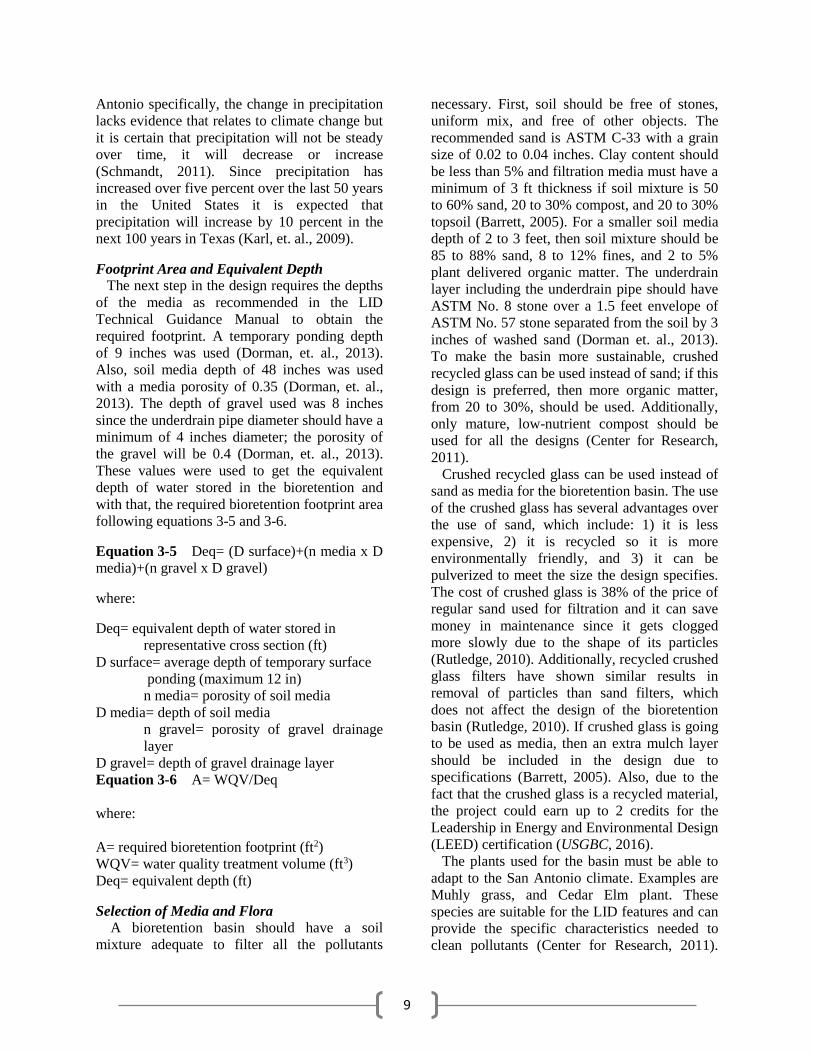
et. al., 2009). Figures 5 to 15 correspond to the

results of the projections and its averages.

Average= 31.6 in/year

Figure 5. Historic Projection 1

y = 0.073x - 112.93 R² = 0.0096

0

10

20

30

40

50

60

1950 1960 1970 1980 1990 2000 2010Ave

rage

Pre

cip

itat

ion

(in

/ye

ar)

Year

Historic Projection 1

11

Average= 27.6 in/yr

Figure 6. Historic Projection 2

Average= 26.1 in/yr

Figure 7. Historic Projection 3

Average= 31.7 in/yr

Figure 8. Historic Projection 4

Average= 22.1 in/yr

Figure 9. Historic Projection 5

y = 0.0303x - 33.58 R² = 0.0032

0

5

10

15

20

25

30

35

40

1950 1960 1970 1980 1990 2000 2010

Ave

rage

Pre

cip

itat

ion

(in

/yr)

Year

Historic Projection 2

y = 0.1622x - 295 R² = 0.0966

0

5

10

15

20

25

30

35

40

45

1950 1960 1970 1980 1990 2000 2010

Ave

rage

Pre

cip

itat

ion

(in

/yr)

Year

Historic Projection 3

y = 0.051x - 69.416 R² = 0.0105

0

10

20

30

40

50

1950 1960 1970 1980 1990 2000 2010

Ave

rage

Pre

cip

itat

ion

(in

/yr)

Year

Historic Projection 4

y = 0.0449x - 66.797 R² = 0.0211

0

5

10

15

20

25

30

35

1950 1960 1970 1980 1990 2000 2010

Ave

rage

Pre

cip

itat

ion

(in

/yr)

Year

Historic Projection 5

12

Average= 28.6 in/yr

Figure 10. Variable Projection 1

Average= 35.2 in/yr

Figure 11. Variable Projection 2

Average= 22.7 in/yr

Figure 12. Variable Projection 3

Average= 34.7 in/yr

Figure 13. Future Projection 1

y = 0.1828x - 347.22R² = 0.0229

0

5

10

15

20

25

30

35

40

45

50

2045 2050 2055 2060 2065 2070

Ave

rage

Pre

cip

itat

ion

(in

/yr)

Year

Variable Projection 1

y = 0.0798x - 128.78 R² = 0.0026

0

5

10

15

20

25

30

35

40

45

50

2045 2050 2055 2060 2065 2070

Ave

rage

Pre

cip

itat

ion

(in

/yr)

Year

Variable Projection 2

y = 0.0062x + 9.9267R² = 9E-05

0

5

10

15

20

25

30

35

2045 2050 2055 2060 2065 2070

Ave

rage

Pre

cip

itat

ion

(in

/yr)

Year

Variable Projection 3

y = 0.4927x - 995.01 R² = 0.1993

0

5

10

15

20

25

30

35

40

45

50

2080 2085 2090 2095 2100

Ave

rage

Pre

cip

itat

ion

(in

/yr)

Year

Future Projection 1

13

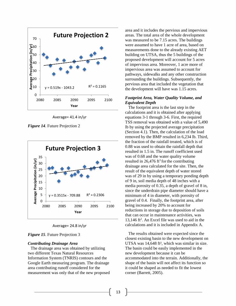
Average= 41.4 in/yr

Figure 14. Future Projection 2

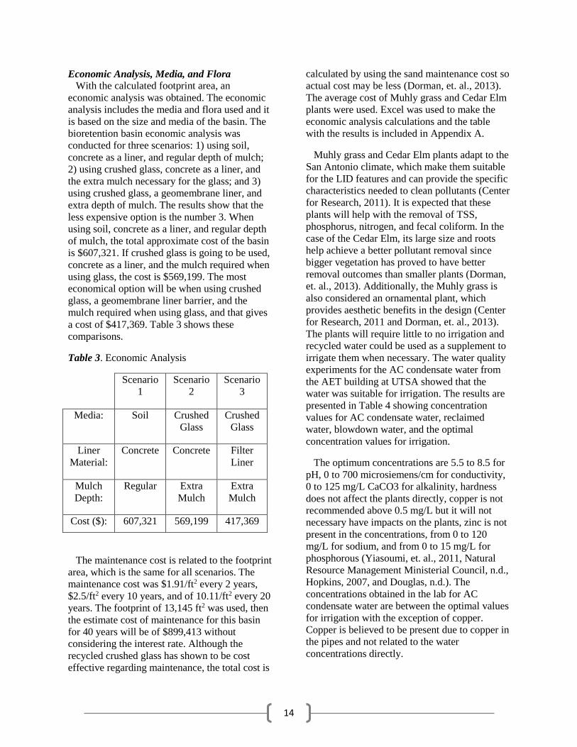
Average= 24.8 in/yr

Figure 15. Future Projection 3

Contributing Drainage Area

The drainage area was obtained by utilizing

two different Texas Natural Resources

Information System (TNRIS) contours and the

Google Earth measuring program. The drainage

area contributing runoff considered for the

measurement was only that of the new proposed

area and it includes the pervious and impervious

areas. The total area of the whole development

was measured to be 7.15 acres. The buildings

were assumed to have 1 acre of area, based on

measurements done to the already existing AET

building on UTSA, thus the 5 buildings of the

proposed development will account for 5 acres

of impervious area. Moreover, 1 acre more of

impervious area was assumed to account for

pathways, sidewalks and any other construction

surrounding the buildings. Subsequently, the

pervious area that included the vegetation that

the development will have was 1.15 acres.

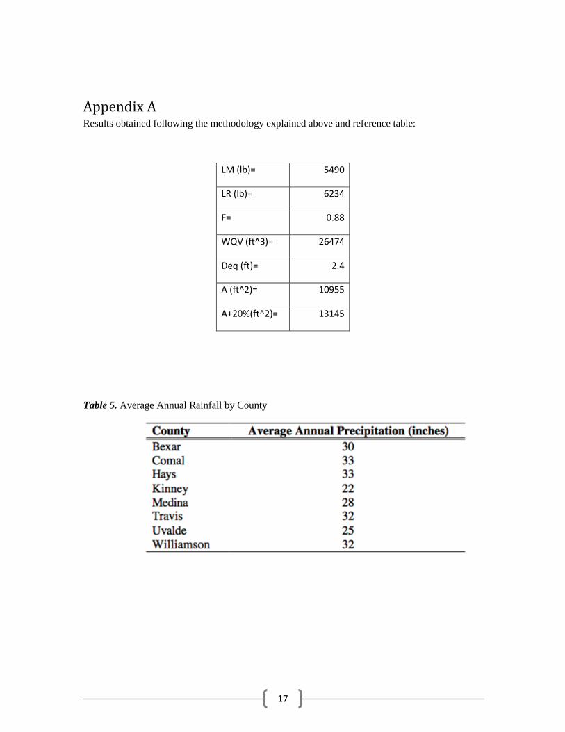
Footprint Area, Water Quality Volume, and

Equivalent Depth

The footprint area is the last step in the

calculations and it is obtained after applying

equations 3-1 through 3-6. First, the required

TSS removal was obtained with a value of 5,490

lb by using the projected average precipitation

(Section 4.1). Then, the calculation of the load

removed by the BMP resulted in 6,234 lb. Third,

the fraction of the rainfall treated, which is of

0.88 was used to obtain the rainfall depth that

resulted in 1.5 in. The runoff coefficient used

was of 0.68 and the water quality volume

resulted in 26,476 ft3 for the contributing

drainage area calculated for the site. Then, the

result of the equivalent depth of water stored

was of 29 in by using a temporary ponding depth

of 9 in, soil media depth of 48 inches with a

media porosity of 0.35, a depth of gravel of 8 in,

since the underdrain pipe diameter should have a

minimum of 4 in diameter, with porosity of

gravel of 0.4. Finally, the footprint area, after

being increased by 20% to account for

reductions in storage due to deposition of soils

that can occur in maintenance activities, was

13,146 ft2. An Excel file was used to aid in the

calculations and it is included in Appendix A.

The results obtained were expected since the

closest existing basin to the new development on

UTSA was 14,648 ft², which was similar in size.

The basin could be easily implemented in the

new development because it can be

accommodated into the terrain. Additionally, the

shape of the basin will not affect its function so

it could be shaped as needed to fit the lowest

corner (Barrett, 2005).

y = 0.519x - 1043.2 R² = 0.1165

0

10

20

30

40

50

60

70

2080 2085 2090 2095 2100

Ave

rage

Pre

cip

itat

ion

(in

/yr)

Year

Future Projection 2

y = 0.3515x - 709.88 R² = 0.2306

0

5

10

15

20

25

30

35

2080 2085 2090 2095 2100

Ave

rage

Pre

cip

itat

ion

(in

/yr)

Year

Future Projection 3

14

Economic Analysis, Media, and Flora

With the calculated footprint area, an

economic analysis was obtained. The economic

analysis includes the media and flora used and it

is based on the size and media of the basin. The

bioretention basin economic analysis was

conducted for three scenarios: 1) using soil,

concrete as a liner, and regular depth of mulch;

2) using crushed glass, concrete as a liner, and

the extra mulch necessary for the glass; and 3)

using crushed glass, a geomembrane liner, and

extra depth of mulch. The results show that the

less expensive option is the number 3. When

using soil, concrete as a liner, and regular depth

of mulch, the total approximate cost of the basin

is $607,321. If crushed glass is going to be used,

concrete as a liner, and the mulch required when

using glass, the cost is $569,199. The most

economical option will be when using crushed

glass, a geomembrane liner barrier, and the

mulch required when using glass, and that gives

a cost of $417,369. Table 3 shows these

comparisons.

Table 3. Economic Analysis

Scenario

1

Scenario

2

Scenario

3

Media: Soil Crushed

Glass

Crushed

Glass

Liner

Material:

Concrete Concrete Filter

Liner

Mulch

Depth:

Regular Extra

Mulch

Extra

Mulch

Cost ($): 607,321 569,199 417,369

The maintenance cost is related to the footprint

area, which is the same for all scenarios. The

maintenance cost was $1.91/ft2 every 2 years,

$2.5/ft2 every 10 years, and of 10.11/ft2 every 20

years. The footprint of 13,145 ft2 was used, then

the estimate cost of maintenance for this basin

for 40 years will be of $899,413 without

considering the interest rate. Although the

recycled crushed glass has shown to be cost

effective regarding maintenance, the total cost is

calculated by using the sand maintenance cost so

actual cost may be less (Dorman, et. al., 2013).

The average cost of Muhly grass and Cedar Elm

plants were used. Excel was used to make the

economic analysis calculations and the table

with the results is included in Appendix A.

Muhly grass and Cedar Elm plants adapt to the

San Antonio climate, which make them suitable

for the LID features and can provide the specific

characteristics needed to clean pollutants (Center

for Research, 2011). It is expected that these

plants will help with the removal of TSS,

phosphorus, nitrogen, and fecal coliform. In the

case of the Cedar Elm, its large size and roots

help achieve a better pollutant removal since

bigger vegetation has proved to have better

removal outcomes than smaller plants (Dorman,

et. al., 2013). Additionally, the Muhly grass is

also considered an ornamental plant, which

provides aesthetic benefits in the design (Center

for Research, 2011 and Dorman, et. al., 2013).

The plants will require little to no irrigation and

recycled water could be used as a supplement to

irrigate them when necessary. The water quality

experiments for the AC condensate water from

the AET building at UTSA showed that the

water was suitable for irrigation. The results are

presented in Table 4 showing concentration

values for AC condensate water, reclaimed

water, blowdown water, and the optimal

concentration values for irrigation.

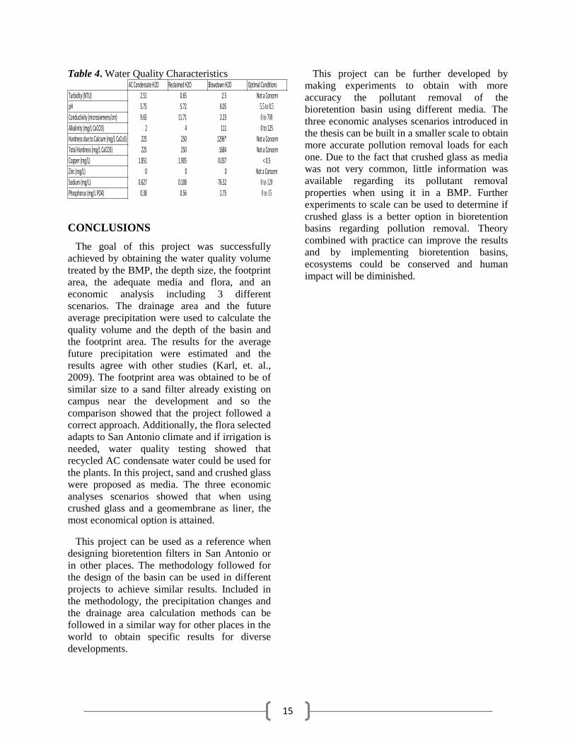
The optimum concentrations are 5.5 to 8.5 for

pH, 0 to 700 microsiemens/cm for conductivity,

0 to 125 mg/L CaCO3 for alkalinity, hardness

does not affect the plants directly, copper is not

recommended above 0.5 mg/L but it will not

necessary have impacts on the plants, zinc is not

present in the concentrations, from 0 to 120

mg/L for sodium, and from 0 to 15 mg/L for

phosphorous (Yiasoumi, et. al., 2011, Natural

Resource Management Ministerial Council, n.d.,

Hopkins, 2007, and Douglas, n.d.). The

concentrations obtained in the lab for AC

condensate water are between the optimal values

for irrigation with the exception of copper.

Copper is believed to be present due to copper in

the pipes and not related to the water

concentrations directly.

15

Table 4. Water Quality Characteristics

CONCLUSIONS

The goal of this project was successfully

achieved by obtaining the water quality volume

treated by the BMP, the depth size, the footprint

area, the adequate media and flora, and an

economic analysis including 3 different

scenarios. The drainage area and the future

average precipitation were used to calculate the

quality volume and the depth of the basin and

the footprint area. The results for the average

future precipitation were estimated and the

results agree with other studies (Karl, et. al.,

2009). The footprint area was obtained to be of

similar size to a sand filter already existing on

campus near the development and so the

comparison showed that the project followed a

correct approach. Additionally, the flora selected

adapts to San Antonio climate and if irrigation is

needed, water quality testing showed that

recycled AC condensate water could be used for

the plants. In this project, sand and crushed glass

were proposed as media. The three economic

analyses scenarios showed that when using

crushed glass and a geomembrane as liner, the

most economical option is attained.

This project can be used as a reference when

designing bioretention filters in San Antonio or

in other places. The methodology followed for

the design of the basin can be used in different

projects to achieve similar results. Included in

the methodology, the precipitation changes and

the drainage area calculation methods can be

followed in a similar way for other places in the

world to obtain specific results for diverse

developments.

This project can be further developed by

making experiments to obtain with more

accuracy the pollutant removal of the

bioretention basin using different media. The

three economic analyses scenarios introduced in

the thesis can be built in a smaller scale to obtain

more accurate pollution removal loads for each

one. Due to the fact that crushed glass as media

was not very common, little information was

available regarding its pollutant removal

properties when using it in a BMP. Further

experiments to scale can be used to determine if

crushed glass is a better option in bioretention

basins regarding pollution removal. Theory

combined with practice can improve the results

and by implementing bioretention basins,

ecosystems could be conserved and human

impact will be diminished.

Turbidity(NTU) 2.51 0.65 2.5

pH 5.75 5.72 8.05Conductivity(microsiemens/cm) 9.65 11.71 2.23Alkalinity(mg/LCaCO3) 2 4 111HardnessduetoCalcium(mg/LCaCo3) 225 250 1296*TotalHardness(mg/LCaCO3) 225 250 1684Copper(mg/L) 1.851 1.905 0.037

Zinc(mg/L) 0 0 0Sodium(mg/L) 0.627 0.108 76.52Phosphorus(mg/LPO4) 0.38 0.56 2.75

0 to 700

0to125

0 to 15

0 to 120

<0.5

NotaConcern

NotaConcernNotaConcern

ACCondensateH2O ReclaimedH2O BlowdownH2O OptimalConditions

5.5 to 8.5

NotaConcern

16

REFERENCES

Center for Research in Water Resources and Lady

Bird Johnson Wildflower Center University

of Texas at Austin. 2011. San Antonio LID

Guidance Manual. Texas Land Water

Sustainability Forum. Texas Commission on

Environmental Quality.

City Council of San Antonio. 1994. The Edward’s

Aquifer: San Antonio Mandates For Water

Quality Protection. San Antonio Water

System. San Antonio, TX.

Barrett, Michael E. 2005. Complying with the

Edwards Aquifer Rules Technical Guidance

on Best Management Practices. Texas

Commission on Environmental Quality.

Center for Research in Water Resources,

University of Texas at Austin.

Dorman, T., M. Frey, J. Wright, B. Wardynski, J.

Smith, B. Tucker, J. Riverson, A. Teague,

and K. Bishop. 2013. San Antonio River

Basin Low Impact Development Technical

Design Guidance Manual, v1. San Antonio

River Authority. San Antonio, TX.

Douglas A. Bailey. “Alkalinity Control for Irrigation

Water used in Greenhouses.” NC State

University, Department of Horticultural

Science n.d. n. pag. Web. 20 January 2016.

Downscaled CMIP3 and CMIP5 Climate and

Hydrology Projections. Lawrence

Livermore National Laboratory, 2014. Web.

1 Feb. 2016.

Economides, Christopher. 2014. Green

Infrastructure: Sustainable Solutions in 11

Cities across the United States. Columbia

University Water Center.

Hopkins, Bryan G. “Managing Irrigation Water

Quality.” Pacific Northwest (2007): n. pag.

Web. 20 January 2016.

Karl, Thomas R., Jerry M. Melillo, and Thomas C.

Peterson. 2009. Global Climate Change

Impacts in the United States. Cambridge

University Press.

Natural Resource Management Ministerial Council.

“Do you know the Quality of your Irrigation

Water?” Vintessential. n.d. n. pag. Web. 20

January 2016.

Office of Mayor Phil Hardberger. 2009. Mission

Verde: Building a 21st Century Economy.

City of San Antonio, Texas.

Rutledge, S. O. “Comparing Crushed Recycled Glass

to Silica Sand for Dual Media Filtration.”

Journal of Environmental Engineering and

Science 1.5 (2010): 927-935. Web. 1 Feb.

2016.

Schmandt, Jurgen, Gerald R. North, and Judith

Clarkson. 2011. The Impact of Global

Warming on Texas. University of Texas

Press.

Texas Commission on Environmental Quality.

Edwards Aquifer. 2008. Web. 27 Sept. 2015.

U.S. Environmental Protection Agency. 2013. Case

Studies Analyzing the Economic Benefits of

Low Impact Development and Green

Infrastructure Programs. Office of

Wetlands, Oceans and Watersheds.

U.S. Global Change Research Program. 2009. Global

Climate Change Impacts in The United

States. Cambridge University Press.

United States Environmental Protection Agency.

2015. Encouraging LID: Incentives Can

Encourage Adoption of LID Practices in

your Community. EPA.

Texas Low Impact Development. 2015.

Guidance Manual.

USGBC. U.S. Green Building Council. Web. 1 Feb.

2016.

Yiasoumi, Bill, Lindsay Evans, and Liz Rogers.

“Irrigation Water Quality” New South

Wales Department of Primary Industries

(2011): n. pag. Web. 20 January 2016.

17

Appendix A Results obtained following the methodology explained above and reference table:

LM (lb)= 5490

LR (lb)= 6234

F= 0.88

WQV (ft^3)= 26474

Deq (ft)= 2.4

A (ft^2)= 10955

A+20%(ft^2)= 13145

Table 5. Average Annual Rainfall by County

18

Biore

tentio

n

Basin

Econ

omic

Anal

ysis:

Dollar/ft^2

Excavation with underdrains: 5 Soil/crushed glass: 5 2 Aggregates: 0.28 Pipe (underdrain): 3.6 Gutter: 18 Mulch: 0.32 0.42 Concrete barrier (liner)/filter fabric: 12 0.45 Vegetation: 2

Mantainance (every 2 years): 1.9

Mantainance (every 10 years): 2.5

Replacement (every 20 years): 10.1

Approximate cost using soil, concrete as a liner, and regular depth of mulch ($):

607321

Approximate cost using crushed sand, concrete as a liner, and mulch required ($): 569199

Approximate cost using crushed sand, concrete as a liner, and mulch required ($): 417369

Mantainance every 2 years ($): 25108 Mantainance every 10 years ($): 32864 Replacement every 20 years ($): 132901

Mantainance every 40 years ($): 899413.1942