DESERTERS, SOCIAL NORMS, AND MIGRATION

by

Dora L. CostaMIT and NBERcosta@mit.edu

Matthew E. KahnThe Fletcher School, Tufts University

matt.kahn@tufts.edu

December 16, 2005

We both gratefully acknowledge the support of NIH grant R01 AG19637 and Dora Costa alsogratefully acknowledges the support of NIH grant P01 AG10120, the Robert Wood JohnsonFoundation, and the Center for Advanced Study in the Behavioral Sciences. The first draft of thispaper was written while the authors were visiting the Center for Advanced Study in theBehavioral Sciences and the economics department at Stanford University, respectively. We thankRobert Ellickson, Joel Sobel, Paul David, Chulhee Lee, Bob Margo, participants at the AEAmeetings, the Hoover bag lunch, and seminars at UC Berkeley, Stanford, and UCLA and thescholars at the Center for Advanced Study for comments. We thank Janet Bassett, JaniceFalconer, Joseph Ferrie, Alexander Glendlin, Adan Haj-Yehia, Melissa Plateck, Larry Wimmer,and Patricia Wimmer for advice and assistance with the 1880 census linkage. We thank AngelaJohnson, Kelly Busby, and Rebecca Lubens for their help in compiling information on state laws.

Deserters, Social Norms, and Migration

ABSTRACT

JEL Classification: Z13

Fourteen percent of Union Army soldiers were deserters. Were these men, who were known in

their home communities to have failed cause and comrades, re-integrated into their communities?

We construct a rich micro panel data set of U.S. Civil War soldiers from pro-war and anti-war

communities to present new evidence on how community social norms shape soldiers’ post-war

experiences. Relative to control groups, deserters were more likely to leave home, particularly if

they were from pro-war communities, to move to anti-war communities, and to re-invent them-

selves by changing their names.

Dora L. CostaMITDepartment of Economics, E52-274C50 Memorial DriveCambridge, MA 02142and NBERcosta@mit.edu

Matthew E. KahnThe Fletcher SchoolTufts UniversityMedford, MA 02155matt.kahn@tufts.edu

1 Introduction

Desertion is the bane of armies. During the U.S. Civil War 9 percent of all Union Army soldiers

deserted. In this war, 14 percent of all Union Army soldiers died, half of them from disease,

and deserters faced minimal legal penalties because Abraham Lincoln knew that in a democracy

“you can’t order men shot by the dozens or twenties. People won’t stand it” (Linderman 1987:

59). Fourteen percent of surviving Union Army soldiers were deserter and, because such a large

fraction of men served in the army, 6 to 11 percent of the Northern male cohorts born between

1835 and 1845 were deserters.1 Were these men, who were known in their home communities to

have failed cause and comrades, re-integrated into their communities?

We construct a rich micro panel data set of civil war soldiers from pro-war and anti-war com-

munities to present new evidence on how community social norms shape soldiers’ post-war ex-

periences. In most empirical settings, norms are notoriously difficult to measure (Durlauf and

Fafchamps 2003). We have a benchmark for community norms, namely their pro-war sentiment.

In previous work (Costa and Kahn 2003), we found that pro-war communities produced fewer

deserters. In this sense, credible social sanctions help bring about social benefits. But, one of the

drawbacks of our previous work was that we could not test how severe the social punishments for

deserters were. In this paper we use new data to find that after the war deserters from such “pro-

war” areas were more likely to change their names and to migrate away from these communities

than observationally identical deserters from ”anti-war” communities. Men who deserted but then

returned to fight behaved like men who never deserted. In our empirical work, we will use these

return deserters as a comparison group for deserters.

This paper first describes the cross-sectional variation in the ”pro-war” norm and its origins

and state variation in laws governing the treatment of deserters. Taking his home community’s

norm and laws as given, in section 3 we discuss the soldier’s choices over desertion and post-

1Estimated from the random sample that we use in the analysis.

1

war migration. Both of these choices are likely to be influenced by the social norm in the home

community. In section 4 we describe our empirical framework and in section 5 we present details of

how we built our unique panel data set. In section 6 we report our hypothesis tests concerning how

social norms shape soldier choices. In section 7, we investigate what factors motivated veterans’

migration choices and in section 8 we conclude.

2 Desertion in the U.S Civil War

Out of roughly 200,000 men who deserted from the Union Army, 80,000 were caught and returned

to the army and 147 were executed for desertion (Linderman 1987: 174, 176). Non-democracies

impose harsher punishments. Out of the roughly 35,000 German soldiers tried for desertion by

the Third Reich, about 22,750 were executed (Knippschild 1998). During the Second World War

not only did Stalin’s armies have special detachments who formed a second line to shoot at any

soldiers in the first line who fled, but the families of all deserters were also arrested (Beevor 1998).

Given the lax formal incentives prevailing in the Union Army and an expected death rate of 14

percent, a rational soldier who feels no shame and fears no social sanction should desert.

The Civil War directly touched all communities. In the Union 65 to 98 percent of the cohorts

born between 1838 and 1845 were examined for military service, and 48 to 81 percent of these

cohorts served, the remainder rejected for poor health. The war affected all social classes within a

community because in this war soldiers were representative of the northern population of military

age in terms of real estate and personal property wealth in 1860 (Fogel 2001) and in terms of

literacy rates (Costa and Kahn 2003a). And in this war local communities had almost complete

information on the daily lives of their men and boys in the military (McPherson 1997).

Although the Civil War ended in 1865, memories of the war left their marks on all communities

and on all veterans. Northern communities began to observe Decoration Day with ceremonies

2

honoring the patriotic dead. Union veterans were viewed by themselves and by Northern civilians

as the country’s saviors who had “preserved for humanity the Republican form of government”

and “elevated the country to a high dignity” (General Daniel Sickles, quoted in McConnell 1992).

Their deeds were commemorated in magazines and newspapers, in generals’ best-selling memoirs,

in regimental histories, in songs, and in public monuments. Union veterans satisfied Victorian

ideals of manhood and self-control and the classical republican ideal of a virtuous citizenry willing

to sacrifice for self-government. They were also God’s chosen instruments for saving the Union

and sweeping away the curse of slavery, permitting the inauguration of a new era (Clarke 2002).

Such a culture could only exacerbate deserters’ personal feelings of shame, particularly if they

were from pro-war communities.

2.1 Spatial Variation in the Support for the Civil War

Local variation in social norms, in our case support for the war, allows us to examine how social

norms shaped soldiers’ post-war choices. We measure support for the war using George McClel-

lan’s share of the vote in the 1864 presidential election as a measure of how anti-war a community

was. The Emancipation Proclamation turned the Civil War into a war against slavery and the 1864

election between Lincoln and McClellan was a referendum on the war. The 1864 Democratic

platform was one of peace without victory, resolving that “immediate efforts be made for a ces-

sation of hostilities” (Long 1994: 283). Secret societies which actively helped northern soldiers

desert, which discouraged enlistments, and which resisted the draft were active in such Democratic

strongholds as the east north central region (Waugh 1997: 211). Counties that previously had been

solidly Republican switched allegiances (e.g. see the case study by Reardon (2002)).

Table 1 presents an analysis of county voting patterns in 1864 and shows that a vote for Mc-

Clellan was an ideological vote, based upon religion. When we divided religions into pietist

(Methodist, Baptist, Congregationalist, Presbyterian, and Unitarian), a group containing many

3

abolitionists who viewed the war as God’s wrath over the curse of slavery (Fogel 1989), litur-

gical (Catholic, Lutheran, and Episcopalian), and other we found that the pro-McClellan counties

were much less likely to be pietist relative to other and much more likely to be liturgical relative to

other. Compared to the coalition voting for Douglas in the 1860 presidential election (results not

shown) the coalition voting for McClellan was even more divided on religious lines.2

Economic interest also explains voting patterns in 1864. Slave-holding counties were more

pro-McClellan. Counties in the Middle Atlantic and in the East North Central Regions were more

likely to be pro-McClellan relative to New England whereas counties in the West North Central

region were even more anti-McClellan than New England.3 In addition, counties where McClellan

received a higher proportion of the vote were poorer, had a lower percentage of their labor force

in manufacturing, and had larger foreign-born populations, particularly Irish and German. Our

empirical work can distinguish between an anti-war vote and purely economic vote because we

can control for county economic characteristics.

2.2 Spatial Variation in Legal Punishment of Deserters

Once the war was over, deserters who had not been pardoned during one of the wartime Presidential

amnesties were dishonorably discharged with forfeiture of pay and could return home without fear

of arrest (Lonn 1928: 202-207; United States War Department. 1880-1901. Series III, Vol. 5,

1900: 110). Although they were deemed by the Federal government to have relinquished their

2In the 1860 election Lincoln owed his narrow victory in part to Yankees who were influenced by the religiousrevival movement that swept the United States in the first half of the nineteenth century and who migrated from NewEngland to the Midwest. Other members of the winning coalition were displaced skilled native-born workers, well-off farmers, and anti-immigrant and anti-Catholic members of the former Know-Nothing party (Fogel 1992). Thecoalition voting for Lincoln was not pro-war in 1860; the initial response to southern secession by anti-slavery forcesin the north, before the firing on Fort Sumter, was to let the “erring sisters go in peace” (Hofstader, Miller, Aaron, andJordan 1976: 285).

3In the east north central region the Civil War severed western-Southern trade along the Ohio and MississippiRivers and local banks, with their holdings of Southern bonds, collapsed, further aggravating existing tensions be-tween Midwestern farmers and the Northeast over protective tariffs and high freight rates (Klement 1999: 43-52).Confederate agents even dreamed of an uprising leading to a western Confederacy (Waugh 1997: 210).

4

citizenship or rights to become a citizen of the United States and thus to have forfeited exercising

any rights of citizens such as voting, this disenfranchisement was widely viewed as ineffectual

because states regulated voting requirements (United States War Department. 1880-1901. Series

III, Vol. 5, 1900: 110). Later court interpretations strengthened this requirement from desertion

to a conviction of desertion.4 However, deserters were disenfranchised in the territories and some

states passed laws disenfranchising deserters.

Our review of state statutes shows that five states disenfranchised deserters: Kansas, Pennsyl-

vania, Wisconsin, New York, and Vermont. In Kansas, an 1866 amendment to the state constitution

revoked voting rights from those dishonorably discharged as well as from felons and people who

had aided in the rebellion, but an 1874 amendment struck dishonorable discharge as one of the

listed offenses that led to a revocation of voting rights. Prior to this amendment, in almost every

year after 1868 voting rights were restored to a list of named men by an act of the state legislature.

An 1866 Pennsylvania law referred to the 1865 act by Congress stating that deserters had forfeited

their US citizenship and in the Pennsylvania Supreme Court case of Huber vs. Reily (53 PA 115)

upheld as constitutional the revocation of citizenship due to desertion but held that because of due

process revocation could only follow upon conviction for court-martial. However, the law may

never have been codified and was not part of the 1873 Digest of Pennsylvania laws. In Wisconsin

an 1866 law allowed election officials to block people challenged as deserters from voting and

an 1867 law ordered the distribution of lists of Wisconsin deserters to election officials in each

precinct who were to post it at every polling place. In 1868 procedures were put in place for an

individual to have his name removed from the deserter list and in 1869 the 1867 law was repealed.

4In the 1875 case of Goetcheus vs Matthewson (61 NY 420) the Court of Appeals of New York decided a casein which the plaintiff sued election officials who had denied him the right to vote in the 1868 election because herefused to answer questions about being a deserter. The defendant-officials claimed that they were charged by thestate constitution with determining the eligibility of voters and the 1865 Federal law authorized them to question theplaintiff about being a deserter. The court held that the 1865 act of Congress only denied the rights of citizens tothose convicted of desertion by a competent court and that election officials were not authorized to determine this factindependently.

5

In 1873 the 1866 law was repealed. In New York an 1867 law providing for a special election of

delegates to a state constitutional convention, required any person seeking to vote in this special

election whose qualifications were challenged to take an oath that, among other things, he had not

willfully deserted from the military. In Vermont an 1866 law disqualified deserters from voting

in city, town, or freemen’s meetings in the date, unless the deserter was pardoned. There is no

evidence of its repeal prior to 1880.

The states disenfranchising deserters were variable in their politics. Kansas and Vermont were

strongly pro-Lincoln states in 1864, with over three-quarters of the population voting for Lincoln.

Lincoln barely carried the states of Pennsylvania and New York and his share of the Wisconsin

vote was equal to his share of the national vote. Although we have no evidence that laws barring

deserters from voting were enforced, we would expect that social norms and the law are likely to

be complements: laws are enforced where people are angry at deserters.

Our empirical work will examine the effect of laws on deserters’ post-war choices. However,

only 5 states passed laws barring deserters from voting and only 3 of those 5 states had strict laws –

Pennsylvania’s law may never have been codified and New York’s law referred to only one election.

Those three states that had strict laws (Vermont, Wisconsin, and Kansas) had small populations.

We therefore expect the effects of laws to be small.

3 Soldiers’ Decisions During and After the War

During the Civil War men first had to decide whether or not to participate in the war. While data

limitations preclude an examination of this decision, combatants resembled the age-adjusted non-

combatant population circa 1860 (Costa and Kahn 2003a). Conditional on participation men then

decided whether or not to desert. We analyzed this decision in Costa and Kahn (2003a). Then men

faced the choice of what to do after the war.

6

In our previous work (Costa and Kahn 2003a), we examined men’s desertion decisions during

the war, finding that if all counties had been as strongly pro-Lincoln as the most pro-Lincoln county

in our sample desertion rates would have fallen from 9 to 8 percent. Both own and community

ideology (we cannot distinguish between the two) could thus increase the economic efficiency of

the military.5

All veterans faced a post-war locational choice. Should they return to their home communities

or move? Consider the migration decision of deserters and non-deserters once the war is over. In

a world of costly information transfer there will be an asymmetry of information across commu-

nities. A deserter’s home town may ostracize and scorn him, and even if it forgave him, he might

be too ashamed to face his friends. But, in a new community a deserter can escape from his past

and re-invent himself because the new town will not know of his war record. In addition, a type

of Tiebout sorting can occur such that deserters seek out more sympathetic (anti-war) communi-

ties. A non-deserter’s migration decision has the familiar economic push and pull factors.6 But,

the non-deserter will face no shame. Shame can therefore be thought of as either a cost to desert-

ers to staying in the home community or as affecting deserters’ expectations of future life in the

community (Elster 1998).

A deserter who feels no shame may still face community ostracism and this creates an incentive

to migrate away. Although choosing heroism or cowardice during the war is a one-shot game,

making strategic sanctioning ineffective, sanctioning could still be motivated by revenge, by a

sense that deserters had not done their fair share, or by the sense that deserters had personally

harmed men who served honorably or the cause they had sacrificed for (Kandel and Lazear 1992;

Fehr and Schmidt 1999; Levine 1998; Rabin 1993).7 Even if deserters felt no connection to their

5We cannot address the issue of who enlists because we do not have a sample of men who did not serve.6He may also Tiebout sort because a non-deserter who started life in an anti-war county might feel mismatched. In

states where soldier and sailor votes were tabulated separately, McClellan received 45 percent of the civilian vote, butonly 22 percent of the military vote in the 1864 presidential election (calculated from Long 1994: 285).

7Dynastic linkage could induce compliance even in short-term interactions. In developing countries today in anoverlapping generation setting potential punishment of children leads to good behavior of the current generation (La

7

home communities and therefore no shame, their consumption would be lower in a community

that imposed economic sanctions. A pro-war community would be more likely to impose such

sanctions. A pro-war community would also be more likely to impose non-pecuniary sanctions

and these would be effective as long as the deserter identified with the home community, in which

case he would feel shame. While we will not be able to explicitly distinguish between shame and

ostracism, we will be able to distinguish between shame and ostracism and economic sanctions.

A soldier might fear future ostracism from his home community because his desertion choice

was well known at home. The potential ostracism and social sanction a deserter would face would

be even stronger in communities that were pro-war and thus had supplied a disproportionately

large number of soliders who fought and died in the war. A necessary condition for a social norm

to influence behavior is that potential norm enforcers have information about who did and did not

violate the norm and that the enforcers have access to credible punishment strategies. During the

Civil War both of these conditions were present. “An enforcer is on the front line of the system

of informal social control. Enforcers observe what actors do and respond by meting out calibrated

social rewards and punishments (Ellickson 2001: 8).” Legal scholars have emphasized a potential

free rider problem. Everyone in a community benefits when the norm enforcers do their job but

they are not explicitly compensated for their actions. Raw emotion and anger at the men who

violate this norm provides a credible mechanism for overcoming this free rider problem. Angry

community members may need no explicit incentive to punish war deserters.

Figure 1 illustrates the sequential decision. A soldier can either desert or not desert. If he

deserts he can either remain a deserter or he can return to fight again, either willingly or under

duress.8 We expect that there would be much less shame in being a returned deserter than in being

a deserter because returned deserters returned to fight until the end of the war. We observe these

Ferrara 2003).8Roughly 25 percent of returned deserters surrendered voluntarily, including those under presidential amnesty

proclamations. The remainder were arrested (Lonn 1928: 179).

8

decisions for everyone in the sample. Once the war is over a soldier can either move or remain

in the home community. Forward looking men who forsaw future ostracism in their community

might adopt an “option value” approach of deserting and then returning home and seeing how they

were treated in their communities.9 Because soldiers had never had the experience of deserting

and then returning to their home communities, they could not predict the consequences of their

action. As this uncertainty was resolved, they could then migrate. Soldiers who move then pick

a new community. We observe these migration decisions for the individuals we are able to link

to the 1880 census, a census which provides us with locational and occupational information on

veterans when their expected median age was 41 and thus when most of their life-cycle migration

was complete.

4 Empirical Framework

The paper’s empirical work focuses on how the probability of migration and the probability of other

post-war outcomes is affected by individual soldiers’ attributes, in particular their war records, and

the communities which they come from. One prediction is that, conditional on our observing a

deserter in the 1880 census, deserters are more likely to leave home, particularly if they are from a

pro-war community. We test this by running probit regressions of the form

Pr(mi = 1) = Φ(β0 + β1Xi + β2RDi + β3Di + β4Ph) (1)

9Official war records support our sequential framework. Lonn (1928: 198-208) reports that during the war bandsof deserters from both sides would roam the territory in or adjacent to the Confederacy where fighting had taken placeand that northern deserters were also particularly likely to be found in Canada, the Territory of Wyoming, and themountainous, wooded, and sparsely settled regions of Pennsylvania. Very few deserters went to the Confederacy.Prior to late 1863, before the federal government actively pursued deserters, deserters would also simply go home.After 1863, deserters fled their home communities for less populated areas. Once the war was over local officialscomplained that their communities were overrun with deserters who had returned home (Lonn 1928: 198-208). Weacknowledge the possibility that a deserter may be more likely to avoid detection in an anti-war home community andthus that self-interest, independent of shame or social sanctions, would push a soldier to such a community. However,as we discuss in the Results section, we find no evidence for this.

9

Pr(mi = 1) = Φ(β0 + β4Xi + β2RDi + β3Di + β4Ph + β5(Di × Ph)) (2)

where m is an indicator variable equal to one if the soldier moved, RD is a dummy variable equal

to one if the soldier was a returned deserter (one who later returned to fight) and D is a dummy

variable equal to one if the soldier was a deserter (non-deserter is the omitted category), Ph is a

measure of the home community’s pro-war sentiment, and X is a vector of individual characteristics

and of state fixed effects. We predict that both β3 and β5 should be greater than zero. If β5 were

less than zero this would mean that deserters from anti-war communities stayed relative to deserters

from pro-war communities. (Since we will be using a measure of anti-war sentiment the coefficient

on β5, our interaction term, will have a negative sign.)

A comparison of migration propensities for deserters and non-deserters may not yield a valid

test for the impact of shame because desertion status is not randomly assigned. While desertion

could cause migration, it could also proxy for other attributes of soldiers. Deserters may be highly

mobile people who cannot commit to either the military or to a specific community. In terms of

observable characteristics deserters were more likely to be married, to be foreign-born, to have

low wealth, and to be illiterate (Costa and Kahn 2003a). Thus differences in human capital are an

alternative explanation for differential migration rates.

We have two approaches for recovering the causal effect of desertion on mobility: 1) using re-

turned deserters as a control group for deserters in the above equations and 2) using an instrumental

variables approach. While returned deserters resemble deserters along key observable characteris-

tics such as wealth and illiteracy rates, they returned to fight and were honorably discharged.

We have a plausible set of instruments for deserter status in measures of company specific

likelihood of death or injury (under the assumption that either war horror and post-war shell shock

are not related or that war horror does not affect post-war migration), in measures of company

specific social capital, and in measures of ideological commitment. A reduced form representation

10

of the soldier’s desertion decision might be written as

D = γ1HC + γ2SC + γ3Horror + U (3)

where a soldier deserts if D > 0. Those highly committed to the cause (HC) are less likely to

desert, but even highly committed men will desert if social capital within their company (SC) is

low enough and if the horrors of war that the company is exposed to are high enough. Soldiers

could also succumb to extreme fear (which can be thought of as temporarily lowering their discount

factor or raising their perceived probability of death), as embodied in the identically independently

distributed error term, U.10

Shame and ostracism also predict that deserters might be more likely to change their names

and re-invent themselves, again particularly if they are from a pro-war community. We therefore

examine what determines the probability that we find a soldier in the 1880 census,

Pr(fi = 1) = Φ(β0 + β1Xi + β2RDi + β3Di + β4Ph + β5Ui) (4)

Pr(fi = 1) = Φ(β0 + β1Xi + β2RDi + β3Di + β4Ph + β5(Di × Ph) + β6Ui) , (5)

where f is an indicator equal to one if we found the soldier and U is an indicator equal to one if

the soldier had an uncommon name. Our finding equations convey both information about who is

likely to hide from the past and they allow us to re-estimate the probability of a move, controlling

for selection (the correlation between our finding equation and our moving equation).

Where do migrants go? Deserters may seek out sympathetic communities controlling for such

state characteristics as distance moved. Alternatively, they may avoid states where they were

10While companies were drawn locally, company characteristics are not highly correlated with county characteris-tics (county heterogeneity can explain only about 3 to 9 percent of the variance in company heterogeneity) and countycharacteristics did not predict desertion. Companies consisted of roughly 100 men and desertion rates were lower inmore homogeneous companies suggesting that social capital in companies reduced shirking. In addition, desertionrates were higher when death rates were higher (Costa and Kahn 2003a).

11

disenfranchised. We estimate the effect of pull factors on the locational decisions of movers as a

function of deserter status using conditional logit models.11 The probability that person i moves to

destination state j conditional that he has moved across states can be written as,

Pr(sij = 1|mi = 1) = F (α0 + β1Pj + β2Xj + β2(Di × Pj) + β3(Di × Pj)) (6)

Pr(sij = 1|mi = 1) = F (α0 + β1Pj + β2Xj + β3(Di × Pj) + β4(Di × Xj)) (7)

where s is the potential state the soldier could move to, i indexes the individual, j indexes the state,

Pj measures how pro-war the state was, Xj is a vector of other state characteristics, and D is a

dummy equal to one if the individual was a deserter.

While both social and economic sanctions yield similar economic predictions, we can test

whether communities imposed economic sanctions on deserters. If communities impose economic

sanctions on deserters then we expect that there will be a monetary penalty to being a deserter.

We test this by examining the occupational transitions of non-deserters, returned deserters, and

deserters.

5 Data

Our data are based upon the military service records of enlisted Union Army soldiers linked back-

wards to the 1860 census.12 The military service records provide information on age at enlistment,

year of enlistment, place of enlistment and also all military service events such as death, injury,

illness, desertion, arrest, AWOL, and discharge. The census records provide information on wealth

and illiteracy and allow us to infer marital status in 1860. As detailed in the Appendix, our sam-

11We do not estimate a nested logit model in which the decision is first whether to stay or to move to another stateand then, for movers, the decision is what state to move to, because the inclusive value would barely differ amongmen. For example, it would be the same for any two men who enlisted in the same state.

12The full set of military service records and of the 1860 census records are available from the Center for PopulationEconomics, http://www.cpe.uchicago.edu, and were compiled by a team of researchers led by Robert Fogel.

12

ple is based upon 20,301 men, known to have survived the war, known not to be dead by 1880,

and with full information on military service dates and on basic demographic characteristics. We

searched for these men in the 1880 census using only name, place of birth, and expected age in

1880 and found 7,224 (36 percent) of them.13 Compared to our initial sample these 7,224 men

were more likely to be native-born, were from richer households, and were less likely to be from

the rapidly growing urban counties. Because we do not know if the individuals we were searching

for were still alive, we cannot determine whether our sample differences are due to mortality at-

trition or to the meticulousness of the census enumerators or the respondents.14 However, in both

samples, we have the full range of socioeconomic and demographic variation.

We restrict our sample to men for whom we can identify county of enlistment, leaving us with

a sample of 18,820 men, 6,549 of whom are linked to the 1880 census with an identifiable 1880

county. Further restricting the sample to men with more complete information on observable char-

acteristics leaves us with 18,274 men, 6,479 of whom are linked to the 1880 census. We examine

both moves across states and moves of at least 350km (a distance larger than the median within

state cross-county move but smaller than the median state move) to control for differences in state

sizes. However, we prefer to focus on state moves because we can then examine how state charac-

teristics affect where migrants go. We classify all men as either non-deserters, returned deserters,

or deserters. Table 2 lists by deserter status the variables we created describing recruits’ individual

characteristics and some of their home community characteristics. In addition to these variables

we also created state fixed effects, dummies for missing individual information, variables describ-

ing company characteristics (which we use as instrumental variables for deserter), and variables

describing the characteristics of the states that were potential destinations for veterans. (See the

Data Appendix for details.)

13Our finding rate compares favorably with linkage rates done with samples that are not in machine-readable form.For example, in linking from the 1850 to 1860 censuses, Ferrie (1996) had a finding rate of 9 percent.

14A post-war death might be reported in pension records if a widow or minor child filed a pension claim, but not allpost-war deaths led to a pension claim.

13

Table 2 shows that, compared to non-deserters, deserters were poorer, were more likely to be

foreign-born, particularly Irish, were less likely to be farmers and more likely to be laborers, were

less likely to be volunteers, were more likely to be married, were more likely to be illiterate, were

less likely to have enlisted early, and were more likely to be from a large town. Returned deserters

resembled non-deserters in terms of birth place and volunteer status and they resembled deserters

in terms of wealth, illiteracy, marital status, and size of city of residence. Returned deserters were

less likely to be farmers than non-deserters but more likely to be farmers than deserters.

6 Results: Migration

Deserters were more likely to move across states between enlistment and 1880 than non-deserters

or returned deserters (see Table 3). Sixty-four percent of deserters moved across states whereas

only 44 percent of non-deserters and 42 percent of returned deserters moved across states.15 De-

serters were also more likely to move further away than non-deserters or returned deserters (see

Figure 2), but deserters who stayed within state were less likely to move across counties (see Ta-

ble 3), suggesting that deserters substituted distant moves for close moves. Note that returned

deserters and non-deserters had almost identical migration propensities. Moving probabilities dif-

fered by the percentage of the vote in the home county for McClellan (see Table 4). In counties

where McClellan received less than 40 percent of the vote, 68 percent of deserters moved across

state compared to 47 percent of non-deserters. But in counties where McClellan received more

than 60 percent of the vote, 58 percent of deserters moved across state compared to 52 percent of

non-deserters. We also observe such differences for the probability of moving at least 350km.

We also calculated differences in the moving propensities of non-deserters, returned deserters,

and deserters by the percentage of the vote cast for McClellan in the 1860 home county. Being in a

15This was a period of high migration rates. In a random sample of men who enlisted in the Union Army we findthat 44 percent of the native-born moved between their state of birth and their state of enlistment.

14

county where McClellan received less than 40 percent of the vote increased deserters’ probability

of moving across states by 0.16 relative to non-deserters and by 0.08 relative to returned deserters.

Deserters’ probability of moving at least 350km increased by 0.13 relative to non-deserters and by

0.14 relative to returned deserters. When deserters did move the state that they moved to was more

pro-McClellan than the state non-deserters moved to and it was also more distant in terms of miles

and in terms of latitude (not shown).

As shown in Table 2, non-deserters, returned deserters, and deserters differed in terms of ob-

servable characteristics. We therefore estimate migration models controlling for these differences.

Table 5, which presents the results from our probit regressions of the probability of moving on

deserter status (Equations 1 and 2), shows that deserters’ probability of moving across states was

higher by a statistically significant 0.135 compared to both non-deserters and returned deserters.16

We find the comparison of deserters with returned deserters quite compelling. Deserters’ proba-

bility of moving at least 350km was higher by 0.115.17 A tobit model shows that, controlling for

all other characteristics, movers who were deserters moved 172.367km (σ=52.439) compared to

non-deserters whereas movers who were returned deserters moved only 1.482km (σ=56.028) com-

pared to non-deserters. When we interact deserter with the logarithm of the percent of the county

vote cast for McClellan we find that a standard deviation increase in the percentage of the vote cast

for McClellan would lower the state migration probability of a deserter by 0.053. Although the

interaction between deserter and the percent of the vote cast for McClellan is only a marginally sta-

tistically significant predictor of moves of at least 350km, the interaction term and deserter status

16We find some evidence that deserters from large cities were less likely to move, perhaps because of the anonymityprovided by large cities. When we interact deserter status with a dummy variable that is equal to one if the deserterenlisted in a city whose population was 50,000 or more in 1860 (one of the 13 largest cities in the US), we find thatin our state move regression the coefficient on deserter is 0.184 (σ =0.035) and that the coefficient on the interactionterm between deserter and our city dummy is -0.111 (σ = 0.069), which barely misses being significantly differentfrom 0 at the 10 percent level. However, the coefficients on deserter and on the interaction term are jointly significantlydifferent from 0 (χ2 =29.88).

17We obtain coefficients of similar magnitude when we run linear probability models with county fixed effects,suggesting that we are not simply measuring county group effects.

15

are highly jointly statistically significant.18 When we restrict the sample to men for whom we had

a higher quality link to the 1880 census, we find that the magnitude of the coefficients is similar,

but the standard error is much larger because of the considerable reduction in sample size.

Deserter status may be correlated with unobserved factors that influence migration (see Equa-

tion 2).19 We therefore instrument for deserter status using 1) such indicators of war horror as the

overall company death rate, the company death rate from disease, the company death rate at spe-

cific times, and dummy indicators of battles and 2) our indicators of war horror plus such company

characteristics as birth place fragmentation, occupational fragmentation, the fraction of a company

of a specific occupation, and the company Gini coefficient for 1860 personal property wealth, and

ideological characteristics such as the percent of the vote received by Lincoln in the 1860 election

in the recruit’s county of enlistment (see the footnote to Table 6 for the full set of instrumental

variables). Our identifying assumption is that war horror, company social capital, and ideology

in 1860 affect desertion but not migration. While war horror which leads to shell shock could

affect the migration decision, we find no evidence that it does. In more homogeneous companies

desertion rates were lower and when company death rates were high desertion rates were higher

too (Costa and Kahn 2003a). Recall that county heterogeneity can explain only 3 to 9 percent of

the variance in company heterogeneity and that companies no longer existed after the war.

Table 6 compares probit and IV probit marginals derived from Equation 1 using non-deserters

as a control group for the combined category of deserters and returned deserters (our instrumental

18Note that the coefficient on the percentage of the vote case for McClellan is not statistically significant, suggestingthat non-deserters (who overwhelmingly voted for Lincoln in 1864) were not alienated from communities that favoredMcClellan.

19If desertion proxies for an unobservable tendency toward high mobility then the coefficient on desertion in theinstrumental variables regression should be smaller than in the simple probit specification. Alternatively, the instru-mental variable results may yield a larger estimated coefficient on deserter status than in the ordinary probit. Supposethat there is a set of soldiers who greatly enjoy living in their pro-war community or whose families are prominent inthe community. The anticipation of shame, including that directed against the entire family, increases the probabilitythat they will not desert in the first place. In this case, our set of deserters is less likely to include men from themost pro-war communities. The ordinary probit would therefore underestimate whether a random soldier assigned“deserter” status would move away.

16

variables predict whether a soldier deserted, but not whether he returned to fight). Because our

instruments are weak, with a first stage pseudo R2 below 0.1, we prefer the simple probit estimates

(Bollen, Guilkey, and Mroz 1995) and view our instrumental variables estimates mainly as a test of

the direction of the bias in using a standard probit.20 The IV marginals on deserter are bigger than

the probit marginals in all cases. Consider the case of moves across state and of moves of at least

350km without controls for county characteristics. In the simple probits the coefficients on deserter

status are 0.10 and 0.09, respectively. When we instrument using our war horror instruments

alone the coefficients increase to 0.40 and 0.31, respectively.21 None of our coefficients shrink,

suggesting that our simple probit results probably underestimate the effect of deserter status on the

probability of migration.

We are less likely to find deserters compared both to non-deserters and returned deserters, sug-

gesting that deserters may have sought to hide their past by changing their names (see Table 7).

Running the regression specified in Equation 4 show that compared to non-deserters, a deserter’s

probability of being found is lower by 0.095. Compared to a returned deserter, a deserter’s prob-

ability of being found is lower by 0.057. When we interact deserter status with the proportion of

the vote for McClellan (see Equation 5) we find that when we control for county characteristics

(or alternatively when we used county fixed effects in a linear probability model), deserters from

counties where McClellan received a larger share of the vote are more likely to be found, but the

effect is small and statistically insignificant. However, deserter status and the interaction of de-

20When we regress desertion status on our war horror instruments alone the pseudo R2 is 0.05 and when we use thefull set of insturements the pseudo R2 is 0.07. We began with a larger set of instruments but excluded some of themas invalid.

21Using the Smith and Blundell (1986) exogeneity test, we reject the hypothesis that desertion status is exogeneous(χ2

1 = 5.169) for state moves but cannot reject the hypothesis that desertion status is exogeneous for moves of at least350km (χ2

1 = 1.846). When we use the full set of instruments we can reject the hypothesis that our instruments areinvalid for state moves in which we control for county heterogeneity, a proxy for community social capital (Costa andKahn 2003b), but we cannot reject the hypothesis for our other specifications. When we include company charac-teristics and ideology as exogeneous regressors in the IV probit and test for the joint significance of these potentialinstruments we obtain a χ2

10 of 15.81, implying that we can reject the hypothesis that our instruments are invalid at the10 percent level.

17

serter status with McClellan’s proportion of the vote is jointly statistically significant. When we

included an interaction between deserter status and a dummy variable indicating that the deserter

was from one of the five states that disenfranchised deserters we found that the derivative of the

coefficient was both qualititatively and statistically indistinguishable from 0.

Our results are robust to controlling for selection. A potential concern is that we can only

measure migration for those we can find. Our finding equation allows us to re-estimate our probit

Equations 1 and 2 controlling for selection using a dummy indicator for uncommon name as the

exclusion restriction. Table 8 shows that the selection correction slightly increases the magnitude

of the coefficient on deserter and on the interaction between deserter and the percentage of the

county voting for McClellan. Returned deserters remained indistinguishable from non-deserters.

When we do not interact deserter with the percentage of the county vote for McClellan we find

that a deserter’s probability of moving across state is 0.142 compared to a non-deserter and that his

probability of moving at least 350km is 0.116 compared to a non-deserter. A standard deviation

increase in the percentage of county vote for McClellan raised a deserter’s probability of a state

move by 0.054.

When deserters did move they sought out a state that was more pro-McClellan compared to

those picked by non-deserters or returned deserters. Table 9, which presents estimates of Equations

6 and 7, shows that controlling for distance from state of enlistment as measured in miles and in

minutes from the enlistment state’s latitude, the odds that a deserter would move to a state were

higher the greater that state’s share of the vote for McClellan. When we controlled for whether

the state had a law disenfranchising deserters and for whether the state was a territory (in which

case federal law was applicable), we found that the odds that a deserter would move a state with a

law disenfranchising deserters were no more greater than those of a non-deserter and that the odds

that a deserter would move to a territory were 1.28 times greater than those of a non-deserter but

that the difference was not statistically significant. A deserter was also more likely to pick a state

18

of a different latitude, because fewer deserters were farmers and therefore did not have skills that

were best used along the same latitude.22 When we restricted the sample to men who were farmers

at enlistment we found no difference in the latitude attributes of the states picked by deserters

and non-deserters. However, deserters continued to pick more pro-McClellan states. When we

examined locational choices by region we found that deserters were not more likely to go to the

states of the former Confederacy, but they were more likely to move to a middle atlantic or east

north central state.

We also used our conditional logit models to determine if returned deserters have the same

preferences as deserters or non-deserters. We ran two different specification, one in which we

interacted the characteristics of the potential destinations with a dummy for returned deserter (ex-

cluding deserters from the sample). Unlike deserters, returned deserters were no more likely to

pick a pro-McClellan state than non-deserters. The coefficient on the interaction term between

returned deserter and the McClellan’s share of the state vote was 0.163 (σ =0.103).

7 Explaining Deserters’ Mobility

Many factors may have explain why deserters’ migration patterns differed from those of non-

deserters, including shame, community ostracism, economic sanctions, legal punishments, or alien-

ation, or simply because they were more mobile individuals. While we cannot directly observe

deserters’ motives, we can rule out the importance of economic and legal sanctions, an inherently

greater mobility, and economic opportunities.

A successful economic boycott of deserters might lead them to fall down the occupational lad-

der, but we find no evidence that between enlistment and 1880 deserters faced a monetary penalty.

Conditional on being a farmer, an artisan, or a laborer upon enlistment χ2 tests indicate that the

22Steckel (1983) documents that migration in the US had traditionally been along the same latitude because farmerscould grow the same crops along the same latitude.

19

occupational transitions of non-deserters, returned deserters, and deserters between enlistment and

1880 were the same (see Table 10). Either communities did not impose economic sanctions on

deserters or by moving to a pro-McClellan state deserters avoided economic penalties. However,

among the small group of men who were professionals or proprietors at enlistment deserters were

less likely to remain professionals or proprietors and were more likely to become artisans and less

likely to become farmers. The data also suggest that the occupational transitions of returned de-

serters resemble those of deserters, but relative to deserters fewer returned deserters were laborers

and more of them remained professionals or proprietors. When we examined the data by state

mover status we found that only for state movers did the 1880 occupational distribution of former

professionals or proprietors differ between deserters and non-deserters, suggesting that profession-

als or proprietors were differentially hurt by a move because their human and social capital may

not have been as easily transferable across states. We also find no evidence that strongly pro-war

communities imposed economic sanctions upon the deserters who did stay.23

We find no evidence that state laws disenfranchising deserters influenced their migration deci-

sions. We augment Equations 2 and 3 by interacting deserter status with a dummy variable indicat-

ing whether a deserter was from one of the 5 states with a law disenfranchising deserters. We find

that the derivative on the probit coefficient was negative and significant ( ∂P∂X

=-0.492, σ=0.155),

suggesting that deserters were less likely to move away from a state with a law disenfranchising

them, and that the coefficients on deserter status and on the interaction between deserter status and

McClellan’s percentage of the vote are still jointly statisticallly significant (χ2 = 30.94). The nega-

tive coefficient on the interaction between deserter status and the law indicator is driven entirely by

Pennsylvania. When we drop this state from the law indicator dummy, we find that the derivative

on the probit coefficient is 0.055 (σ=0.677).

23When we examine men who did not move across state and who were from counties where McClellan receivedless than 40 percent of the vote, then, conditional upon occupational class at enlistment, the occupational distributionsof non-deserters and deserters were statistically indistinguishable.

20

Deserters might simply be highly mobile people. We tested for this by restricting the sample

to the native-born and controlled for whether the veterans had migrated between state of birth and

state of enlistment (a proxy for mobility), we found that, compared to non-deserters, deserters’

probability of migrating out of state was 0.111 (σ =0.034) and that returned deserters’ probability

of migrating out of state was -0.019 (σ =0.041), coefficients virtually identical to those obtained

without controlling for our mobility proxy. Deserters’ greater mobility could not be explained by

their better health capital. When we controlled for whether or not the soldier was wounded or for

length of time served, our coefficients remained virtually unchanged.

Deserters’ greater mobility does not reflect conditions in the states, counties, or companies

they were from. All of our regressions included state fixed effects. When we ran linear probability

models in which we included county fixed effects, deserters’ probability of migrating out of state

relative to non-deserters rose to 0.163 (σ =0.028).24 When we ran linear probability models that

included company fixed effects we found that in the state mover specification with no interactions

the coefficient on deserter was 0.140 (σ =0.031).25

Deserters’ locational choice in 1880 does not reflect their efforts to avoid detection during the

war. Roughly 75 percent of returned deserters were arrested. But, when we restricted the sample

to deserters and returned deserters and ran a probit in which the dependent variable is a dummy

equal to one if the soldier was a returned deserter and in which we control for the logarithm

of McClellan’s share of the vote, individual characteristics, and for region, we found that the

coefficient on the vote for McClellan was small and statistically insignificant, suggesting that there

was no difference in detection rates in pro-McClellan and pro-Lincoln counties.

24When we included an interaction term between the logarithm of the percentage voting for McClellan and deserterstatus the coefficient on deserter status rose to 0.553 (σ =0.220) and the coefficient on the interaction term was -0.102(σ =0.057).

25When we included an interaction term of deserter with the logarithm of the percentage voting for McClellan wefound that the coefficient on deserter was 0.496 (σ =0.134) and that the coefficient on the interaction term was -0.093(σ =0.036).

21

8 Conclusion

Diaries, letters, and newspaper accounts from the antebellum era have not left a paper trail of how

deserters fared after the war. Our unique panel data set allowed us to discover that faced with the

choice of returning home or of moving and re-inventing themselves, deserters moved. Compared

to a non-deserter, a deserter’s probability of leaving his state by 1880 was higher by at least 0.135

and his probability of moving at least 350km was higher by 0.115. Deserters from pro-war com-

munities were more likely to move than deserters from anti-war communities and when deserters

moved they were more likely to move to anti-war states. Perhaps it is no accident that the fate

of deserters is not mentioned in contemporary accounts. As we observe in countries making a

transition to democratic rule, there is a desire to avoid painful confrontations after traumatic na-

tional events, particularly if a sizable proportion of the population behaved shamefully (Barahona

de Brito et al. 2001; Paxton 1998). Transitions are also accompanied by the creation of national

epics which provide legitimization for the creation of a new state and national identity (Lagrou

2000). These national myths may persist for a long time. Lonn’s (1928) study of desertion in the

Civil War pointed out that “the knowledge of any desertion in the brave ranks of the armies ... will

come as a distinct shock” and that “the average reader will question the worth-whileness of an

exhaustive study of that which seems to record a nation’s shame” (p. v).

Data Appendix

Our sample is drawn from a dataset of 35,570 white, enlisted men in 303 Union Army infantry

companies, representing roughly 1.3 percent of all whites mustered into the Union Army and 8

percent of all regiments that comprised the Union Army.26 The primary data source consists of

26The data were collected by Robert Fogel and are available from http://www.cpe.uchicago.edu. The 303 companiesare part of a sample of 331 companies, picked at random with one hundred percent sampling of all of the enlisted men.Our sample is limited to 303 companies because complete data have not yet been collected on all 331 companies.Among the original 331 companies, New England is under-represented and the Midwest over-represented relative to

22

men’s military service records. These records provide such basic information as year of muster,

age, birthplace, and height in inches, and also information on what happened to the soldier during

his military service such as death, injury, illness, desertion, arrest, or AWOL. These 35,570 men

were linked to the manuscript schedules of the 1860 census which provides information on the

value of personal property for all individuals in the household and on illiteracy and allows us to

infer marital status.

Sample Construction

We take the sample of 35,570 men and restrict it to men who survived the war, men not known

to have died before 1880, men with information on date of discharge, desertion, or other events

that led them to leave the company (necessary for distinguishing between returned deserters and

deserters), and men with consistent and non-missing information on such basic characteristics as

birth place and age at enlistment or birth year. This leaves us with a sample of 20,301 men, 36

percent of whom (7,224) we can link to the 1880 census. (We later further restrict the sample to

men with identifiable county information in 1860.) Our linkage procedure used a combination of

computerized and manual procedures. We obtained computerized lists of potential census matches

based upon a last name matching the soundex and a match of the first letter of either the first or

middle name from the Center for Population Economics at the University of Chicago and restricted

the lists to those whose age in 1880 was within ten years of the expected age of our veterans,

to those who were born in the same state or foreign country, and to white males. If, after our

restrictions, the list of potential matches was still greater than 40 we classified these men as not

found and did not search any further for them. If the list of potential matches was less than 40

trained genealogists decided whether a name was a potential match. The genealogists classified all

matches as 1) good, 2) possible, 3) possible plus, and 4) not found. A “good” match was one where

the army as a whole. The companies that have not yet been collected are from Indiana and Wisconsin, states that werevery committed to the Union cause.

23

there existed only a single match to a given name and surname. A “possible” match was one where

either a) there were two or three possible matches to a given name and surname but only one match

was within 2 years of the expected age of the veteran in 1880; b) there was a match to the surname,

but the given name, while not exact, was a possible alternative name; or, c) there was match to the

surname but instead of the given name, only the proper initial was listed. A “possible plus” match

was one where the matched name fit the criteria for a possible match but because the name was

significantly unusual or because of some other special consideration the possibility of a match was

deemed better than possible but short of good. A “not found” match was one where either none

of the choices was an acceptable match or when there were several possible matches, all equally

good. Among the men who were found, 65 pecent of them were “good” matches, 30 percent of

them were “possible” matches, and the remaining 5 percent were “possible plus” matches.

We were able to test the quality of our matches by comparing our matching with that done

by the Center for Population Economics at the University of Chicago to the 1880 census using

information from the pension records (and therefore excluding deserters). We found that among

men who were both in their and in our linked dataset we had the same match in 97 percent of all

cases and a different match in the remaining 3 percent of cases. Because our linkage procedure

was based upon limited information, we could not find 33 percent of the men in the linked Center

for Population Economics data.

The sample of 20,301 men whom we tried to link to the 1880 census was slightly richer than the

original sample of 35,570 men who served in the Union Army. Median total household personal

property wealth in 1860 was $150 dollars and controlling for age and region a median regression

in which the logarithm of total household property wealth was the dependent variable revealed that

total household personal property wealth was lower by a statistically significant $16 in our sample

of 20,315. However, total household real estate wealth was the same in both samples.

Our sample of 7,224 men linked to the 1880 census differs from our initial sample in several

24

ways. A probit regression of the finding probability showed that the foreign born, particularly the

Irish, were less likely to be found. Laborers were less likely to be found than farmers, professionals

or proprietors, or artisans. Those who lived in households with higher total personal property

wealth in 1860 were more likely to be found. Census enumerators may have been less meticulous

in accurately recording the names, places of birth, and ages of the poor and foreign-born and

in enumerating them and the foreign-born and the poor may have given census enumerators less

accurate information. In addition, if mortality rates were higher among the foreign-born and the

poor, we would be less likely to find them. To our surprise, men who enlisted in counties with

higher percentages of the foreign-born and of workers in manufacturing and with a large city of at

least 50,000 people in the county were less likely to be found. We suspect that in such counties

either individuals or census enumerators in 1880 were less careful or that we are measuring an

urban mortality penalty.

Variables

Dependent Variables

Our empirical work uses several dependent variables. We examine migration using a dummy

variable equal to one if the veteran moved across states between 1860 and 1880 and a dummy

variable equal to one if he moved at least 350km (as measured at the county centroid) between

those years. We investigate the determinants of our finding a veteran in the 1880 census using a

dummy equal to one if we find the veteran. We examine what state a veteran moves to conditional

on his being a mover using an indicator variable for all 48 mainland states.

Socio-economic and Demographic Characteristics

1. Occupation. Dummy variables indicating whether at enlistment the recruit reported hisoccupation as farmer, artisan, professional or proprietor, or laborer. Farmers’ sons who werenot yet farmers in their own right would generally report themselves as farmers.

25

2. Birth place Dummy variables indicating whether at enlistment the recruit reported his birthplace as the US, Germany, Ireland, Great Britain, Canada, or other.

3. Age at enlistment. Age at first enlistment.

4. Married in 1860. This variable is inferred from family member order and age in the 1860census. This variable was set equal to 0 if the recruit was not linked to the 1860 census.

5. Log(total household personal property) in 1860. This variable is the sum of personalproperty wealth of everyone in the recruits’ 1860 household. This variable is set equal to 0is the recruit was not linked to the 1860 census.

6. Missing census information. A dummy equal to one if the recruit was not linked to the1860 census. Linkage rates from the military service records to the 1860 census were 57percent. The main characteristic that predicted linkage failure was foreign birth.

7. Illiterate. This variable is from the 1860 census and provides illiteracy information only forthose age 20 and older.

8. Missing illiteracy information. A dummy equal to one if we do not know whether therecruits was illiterate, either because he was not linked to the 1860 census or because he wasless than age 20 in 1860.

9. Year of muster. Dummy variables indicating the year that the soldier was first mustered in.

10. Volunteer. A dummy equal to one if the recruit was a volunteer instead of a draftee or asubstitute.

11. Bounty. We create a dummy variable equal to one if a recruit received a bounty uponenlistment and a dummy variable equal to one if a recruit was owed a bounty upon hisreturn. Bounties for enlistment were offered by Congressional districts after mid-1862 whencounties had difficulty meeting their recruiting quotas.

12. Uncommon name. A dummy equal to one if the soldier had an uncommon surname, thatis one that appears less than four times in the 1880 integrated public use census sample,http://www.ipums.umn.edu. We thank the Center for Population Economics at the Universityof Chicago for this variable.

City, County, and State Characteristics

1. Population in city of enlistment. We obtained population in city of enlistment from UnionArmy Recruits in White Regiments in the United States, 1861-1865 (ICPSR 9425), RobertW. Fogel, Stanley L. Engerman, Clayne Pope, and Larry Wimmer, Principal Investigators.Cities that could not be identified were assumed to be cities of population less than 2,500.

26

2. Percent of vote for McClellan in the 1864 Presidential election. We obtained by countyof enlistment the percent of the vote for McClellan from Electoral Data for Counties in theUnited States: Presidential and Congressional Races, 1840-1972 (ICPSR 8611), JeromeM. Clubb, William H. Flanigan, and Nancy H. Zingale, Principal Investigators. If votinginformation is unavailable for a county, then for counties in the Confederacy we attributed a90 percent share of the vote to McClellan and for other counties we attributed a 0 percent ofthe vote to McClellan. We therefore also include a dummy variable indicating that in thesetwo cases the share of the vote for McClellan is unknown. We use our county data to obtainstate-wide voting percentage for McClellan, weighted by the total number of votes cast ineach county.

3. County Characteristics We obtain information on the share of the population that wasforeign born, on the share of the population in manufacturing, and on average personal prop-erty and land wealth from Historical, Demographic, Economic, and Social Data: The UnitedStates, 1790-1970 (ICPSR 3), Inter-University Consortium for Political and Social Research,Principal Investigator. We obtain information on county birth place and occupational frag-mentation, on county birth place composition, and on whether a county contained a citywhose population was at least 50,000 from the 1860 integrated public use census sample,http://www.ipums.umn.edu.

4. State law. We examined the statutes of all states from 1865 to 1880 and noted laws gov-erning deserters. We constructed a dummy variable indicating whether a state had lawsgoverning the voting rights of deserters and also a dummy variable indicating whether a“state” was a territory in which federal law applied.

5. State fixed effects. We include state fixed effects in our regressions in Tables 5, 6, 7, and 8.

6. Other state characteristics. For every state the soldier could potentially move to, we esti-mate its distance from his home state in miles and in latitude minutes, calculated from thestate centroid.

Company Characteristics

We use company characteristics and ideology as instrumental variables for whether an individualwas a deserter. The company characteristics (estimated for the full sample of 35,570 men) thatwe use are birth place fragmentation (calculated for the categories New England, Middle Atlantic,East North Central, West North Central, Broder, South, West, Canada, Germany, Ireland, GreatBritain, Scandinavia, northwestern Europe, other European, and other foreign); occupational frag-mentation (calculated for the categories farmer, higher class professionals and proprietors, lowerclass professional and proprietors, artisans, upper working class laborer, lower class laborer, andunknown); the coefficient of variation in age at enlistment; the percent of the company that died;the percent of the company that died from illness; the percent of the company that died within 6month intervals; dummy indicators for battles (First Battle of Bull Run, Shiloh, Second Battle of

27

Bull Run, Antietam, Fredricksburg, Chancellorville, Vicksburg, Gettysburg, Chickamauga, Chat-tanooga, Seven Days, Cold Harbor, Wilnderness, Spotsylvania, Stone River, Atlanta, KennesawMountain, Petersburg, and the March to the Sea); the percent voting for Lincoln in 1860 in thesoldier’s county of enlistment; the occupational composition of the company (percent professionalor proprietor, artisan, laborer, and farmer as the omitted category); and the Gini coefficient fortotal household personal property wealth in 1860. When the Gini coefficient was unavailable (be-cause too few soldiers in the company were linked to the 1860 census), the Gini coefficient was setequal to 0 and a dummy variable indicating that the Gini coefficient was missing was used in theregression.

References

[1] Barahona de Brito, Alexandra, Carmen Gonzalez-Enrıquez, and Paloma Aguilar, Eds., 2001.The Politics of Memory: Transitional Justice in Democratizing Societies. Oxford-New York:Oxford University Press.

[2] Bollen, Kenneth A., David K. Guilkey, and Thomas A. Mroz. 1995. “Binary Outcomes andEndogeneous Explanatory Variables: Tests and Solutions with an Application to the Demandfor Contraceptive Use in Tunisia.” Demography. 32(1): 111-31.

[3] Clarke, Frances. 2002. “‘Honorable Scars’: Northern Amputees and the Meaning of CivilWar Injuries.” In Paul A. Cimbala and Randall M. Miller, Eds, Union Army Soldiers and theNorthern Home Front. New York: Fordham University: 361-394.

[4] Costa, Dora L. and Matthew E. Kahn. 2003a. “Cowards and Heroes: Group Loyalty Duringthe American Civil War.” Quarterly Journal of Economics. 118(2): 519-548.

[5] Costa, Dora L. and Matthew E. Kahn. 2003b. “Understanding the American Decline in SocialCapital, 1952-1998.” Kyklos. Fasc. 1. 56(1): 17-46.

[6] Durlauf, Steven N. and Marcel Fafchamps. 2003. “Empirical Studies of Social Capital: ACritical Survey.” University of Wisconsin Working Paper No. 12.

[7] Ellickson, Robert C. 2001. “The Market for Social Norms.” American Law and EconomicsReview. 3(1): 1-49.

[8] Elster, Jon. 1998. “Emotions and Economic Theory.” Journal of Economic Literature. 36:47-74.

[9] Fehr, Ernst and Klaus M. Schmidt. 1999. “A Theory of Fairness, Competition, and Coopera-tion.” Quarterly Journal of Economics. 114(3): 817-68.

28

[10] Ferrie, Joseph P. 1996. “A New Sample of Males Linked from the Public Use Micro Sampleof the 1850 U.S. Federal Census of Population to the 1860 U.S. Federal Census ManuscriptSchedules.” Historical Methods. Fall. 29: 141-156.

[11] Fogel, Robert William. 1989. Without Consent or Contract: The Rise and Fall of AmericanSlavery. New York: W.W. Norton and Company.

[12] Fogel, Robert W. 1992. “Problems in Modeling Complex Dynamic Interactions: The PoliticalRealignment of the 1850s.” Economics and Politics. 4(3): 215-254.

[13] Fogel, Robert W. 2001. “Early Indicators of Later Work Levels, Disease, and Death.” Grantsubmitted to NIH, February 1, 2001.

[14] Hofstader, Richard, William Miller, Daniel Aaron, and Winthrop D. Jordan. 1976. The UnitedStates: Conquering A Continent. Englewood Cliffs, NJ: Prentice-Hall.

[15] Kandel, Eugene and Edward P. Lazear. 1992. “Peer Pressure and Partnerships.” Journal ofPolitical Economy. 100(4): 801-817.

[16] Klement, Frank L. 1999. Lincoln’s Critics: The Copperheads of the North. Shippensburg,PA: White Mane Books.

[17] La Ferrara, Eliana. 2003. “Kin Groups and Reciprocity: A Model of Credit Transactions inGhana.” American Economic Review. 93(5): 1730-51.

[18] Levine, David K. 1998. “Modeling Altruism and Spitefulness in Experiments.” Review ofEconomic Dynamics. 1: 593-622.

[19] Linderman, Gerald F. 1987. Embattled Courage: The Experience of Combat in the AmericanCivil War. New York: The Free Press.

[20] Long, David E. 1994. The Jewel of Liberty: Abraham Lincoln’s Re-Election and the End ofSlavery. Mechanicsburg, PA: Stackpole Books.

[21] Lonn, Ella. 1928. Desertion During the Civil War. New York-London: The Century Co.

[22] McConnell, Stuart. 1992. Glorious Contentment: The Grand Army of the Republic, 1865-1900. Chapel Hill, NC and London: The University of North Carolina Press.

[23] Paxton, Robert 0. 1998. “Foreword.” In Eric Conan and Henry Rousso, Authors, Vichy: AnEver-Present Past. Hanover, NH and London: Dartmouth University Press, pp. ix-xiii.

[24] Putnam, Robert. 2000. Bowling Alone. New York: Simon and Schuster.

[25] Rabin, Matthew. 1993. “Incorporating Fairness into Game Theory and Economics.” AmericanEconomic Review. 83(5): 1281-302.

29

[26] Reardon, Carol. 2002. “ ‘We Are All in This War’: The 148th Pennsylvania and Home FrontDissension in Centre County during the Civil War.” In Paul A. Cimbala and Randall M.Miller, Eds, Union Army Soldiers and the Northern Home Front. New York: Fordham Uni-versity: 3-29.

[27] Smith, Richard J. and Richard W. Blundell. 1986. “An exogeneity test for a simultaneousequation Tobit model with an application to labor supply.” Econometrica. 54(4): 679-86.

[28] Steckel, Richard H. 1983. “The Economic Foundations of East-West Migration during the19th Century.” Explorations in Economic History. 20(1): 14-36.

[29] United States. War Department. 1880-1901. The War of the Rebellion: A Compilation of theOfficial Records of the Union and Confederate Armies. Govertment Printing Office: Wash-ington DC.http://cdl.library.cornell.edu/moa/browse.monographs/waro.html

[30] Waugh, John C. 1997. Re-Electing Lincoln: The Battle for the 1864 Presidency. New York:Crown Publishers.

30

Table 1: Determinants of Vote for McClellan in 1864

Coefi- Std Oddscient Err Ratio

% of church seats held byPietist sects -0.454‡ 0.117 0.635Liturgical sects 0.356† 0.183 1.428Other sects

% of labor force in manufacturing -0.700‡ 0.269 0.497Dummy=1 if county above county mean for

Personal property wealth -0.024 0.040 0.976Real estate wealth -0.082† 0.039 0.921

% of free population slave-owners 0.159‡ 0.025 1.172% of free population born in

United StatesIreland 0.009† 0.004 1.010Britain -0.025‡ 0.006 0.975Germany 0.013‡ 0.003 1.013Other foreign -0.011‡ 0.004 0.989

Logarithm of county population -0.053† 0.026 0.948Dummy=1 if region

New EnglandMiddle Atlantic 0.506‡ 0.062 1.659East North Central 0.304‡ 0.074 1.355West North Central -0.199‡ 0.097 0.820Border 0.115 0.133 1.122West 0.110 0.126 1.116

Constant 0.374 0.269

Results are from a weighted generalized least squares regression in which the dependent variable is log(Mi/(100 −Mi)), where Mi is the percentage of the vote cast for McClellan. County characteristics are county characteristicsin 1860. 941 observations. Adjusted R2 =0.223. Our electoral data come from Electoral Data for Counties inthe United States: Presidential and Congressional Races, 1840-1972 (ICPSR 8611), Jerome M. Clubb, William H.Flanigan, and Nancy H. Zingale, Principal Investigators. Our county characteristics are from Historical, Demographic,Economic, and Social Data: The United States, 1790-1970 (ICPSR 3), Inter-University Consortium for Political andSocial Research, Principal Investigator, with the exception of the percent born in a particular birthplace which weestimated from the 1860 integrated public use census sample, http://www.ipums.umn.edu. The symbols ∗, †, and ‡indicate significance at the 10, 5, and 1 percent level, respectively.

31

Table 2: Characteristics of Non-Deserters, Returned Deserters, and Deserters in the Initial Sampleand in the Found Sample

Initial Sample Found SampleNon- Returned Non- Returned

Deserters Deserters Deserters Deserters Deserters DesertersPercent of sample 0.872 0.033 0.095 0.917 0.028 0.055

Dummy=1 if born inUnited States 0.679 0.680 0.430 0.764 0.759 0.638Ireland 0.088 0.121 0.209 0.028 0.049 0.087Britain 0.038 0.049 0.084 0.033 0.038 0.064Germany 0.088 0.075 0.099 0.069 0.082 0.098Canada 0.034 0.036 0.074 0.031 0.049 0.067Other foreign country 0.073 0.039 0.104 0.075 0.023 0.046

Dummy=1 if occupation at enlistmentFarmer 0.491 0.381 0.247 0.555 0.497 0.335Professional or proprietor 0.082 0.085 0.097 0.075 0.066 0.103Artisan 0.209 0.282 0.257 0.204 0.251 0.249Laborer 0.210 0.249 0.392 0.157 0.186 0.310Unknown 0.008 0.003 0.007 0.009 0.000 0.003

Dummy=1 if volunteer 0.894 0.892 0.788 0.916 0.896 0.852Dummy=1 if received bounty 0.311 0.289 0.249 0.315 0.273 0.249Dummy=1 if owed bounty 0.178 0.157 0.182 0.176 0.115 0.190Household personal property wealth ($) 581 384 429 635 442 365Dummy=1 if married in 1860 0.306 0.366 0.388 0.296 0.333 0.291Dummy=1 if illiterate 0.034 0.063 0.070 0.032 0.053 0.035Dummy=1 if enlisted in

1861 0.205 0.298 0.127 0.196 0.300 0.1321862 0.324 0.384 0.299 0.350 0.393 0.3211863 0.060 0.067 0.170 0.047 0.066 0.1481864 0.262 0.148 0.217 0.264 0.164 0.2151865 0.149 0.103 0.187 0.143 0.077 0.184

Dummy=1 if uncommon name 0.472 0.434 0.391 0.539 0.574 0.4611860 Population in city of enlistment 76,286 147,160 127,669 49,611 103,375 100,549Percentage of county vote for McClellan 45.76 49.68 49.35 44.44 48.16 48.11

32

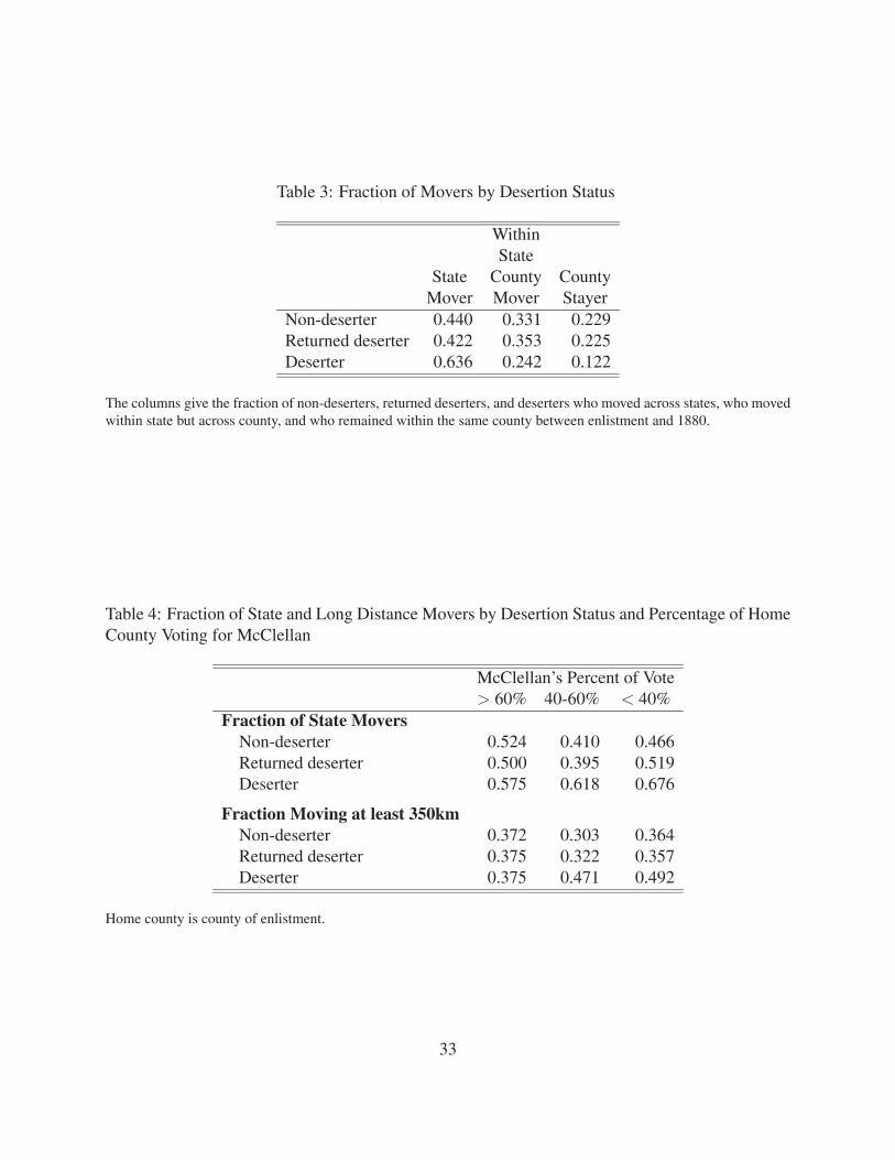
Table 3: Fraction of Movers by Desertion Status

WithinState

State County CountyMover Mover Stayer

Non-deserter 0.440 0.331 0.229Returned deserter 0.422 0.353 0.225Deserter 0.636 0.242 0.122

The columns give the fraction of non-deserters, returned deserters, and deserters who moved across states, who movedwithin state but across county, and who remained within the same county between enlistment and 1880.

Table 4: Fraction of State and Long Distance Movers by Desertion Status and Percentage of HomeCounty Voting for McClellan

McClellan’s Percent of Vote> 60% 40-60% < 40%

Fraction of State MoversNon-deserter 0.524 0.410 0.466Returned deserter 0.500 0.395 0.519Deserter 0.575 0.618 0.676

Fraction Moving at least 350kmNon-deserter 0.372 0.303 0.364Returned deserter 0.375 0.322 0.357Deserter 0.375 0.471 0.492

Home county is county of enlistment.

33

Table 5: Effect of Deserter Status on the Probability of State and Long Distance Moves

State Mover ≥350km Mover∂P∂x

∂P∂x

∂P∂x

∂P∂x

Non-deserterReturned deserter -0.016 -0.017 0.006 0.007

(0.035) (0.036) (0.028) (0.030)Deserter 0.135‡ 0.409‡ 0.115‡ 0.379‡

(0.034) (0.118) (0.037) (0.149)Log(% county vote for McClellan) 0.004 -0.003 -0.000 -0.023

(0.018) (0.027) (0.017) (0.028)Deserter×Log(%county vote for McClellan) -0.149‡ -0.107∗

(0.059) (0.059)χ2(2) for test of joint significance of Deserter

and Deserter×Log(%county vote for McClellan) 27.88 30.13Prob > χ2 0.000 0.000

Pseudo R2 0.074 0.075 0.075 0.075

Coefficients are the mean derivatives from a probit regression in which the dependent variable is equal to one ifthe soldier moved between states or at least 350km and 0 otherwise. Additional control variables include age atenlistment, dummy variables for place of birth (US, Ireland, Britain, Germany, Canada, and other), dummy variablesfor occupation at enlistment (farmer, professional or proprietor, artisan, laborer, and unknown), a dummy equal to oneif the soldier volunteered, a dummy equal to one if the soldier received a bounty at enlistment, a dummy equal toone if the soldier was owed a bounty upon his return, the logarithm of personal property wealth in 1860, a dummyequal to one if the soldier was illiterate, a dummy equal to one if the soldier was married in 1860, the logarithm ofpopulation in the city of enlistment, dummies equal to one if information on county voting was missing, if informationon literacy was missing, and if the soldier was not linked to the 1860 census, dummies for year of enlistment, anddummies for state of enlistment. Robust standard errors clustered on the county of enlistment are in parentheses.6,479 observations. The symbols ∗, †, and ‡ indicate significance at the 10, 5, and 1 percent level, respectively.

34

Table 6: Effect of Deserter Status on the Probability of State and Long Distance Moves, Compari-son of Probit and IV Probit Results

State Mover ≥350km Mover(1) (2) (1) (2)IV IV IV IV

Probit Probit Probit Probit Probit Probit∂P∂x

∂P∂x

∂P∂x

∂P∂x

∂P∂x

∂P∂x

Without County CharacteristicsDeserter 0.097‡ 0.398‡ 0.409‡ 0.089‡ 0.315 0.161

(0.024) (0.125) (0.121) (0.023) (0.214) (0.178)

Pseudo R2 0.072 0.072 0.071 0.073 0.074 0.072With County Characteristics

Deserter 0.095‡ 0.479‡ 0.438‡ 0.088‡ 0.292 0.170(0.024) (0.117) (0.117) (0.023) (0.214) (0.188)

Pseudo R2 0.076 0.071 0.076 0.074 0.075 0.074

Deserters include returned deserters. Probit estimates are the mean derivatives from a probit regression in which thedependent variable is equal to one if the soldier moved between states or moved at least 350km and 0 otherwise. Addi-tional control variables include the percentage of the county voting for McClellan in 1864, age at enlistment, dummyvariables for place of birth (US, Ireland, Britain, Germany, Canada, and other), dummy variables for occupation atenlistment (farmer, professional or proprietor, artisan, laborer, and unknown), a dummy equal to one if the soldiervolunteered, a dummy equal to one if the soldier received a bounty at enlistment, a dummy equal to one if the soldierwas owed a bounty upon his return, the logarithm of personal property wealth in 1860, a dummy equal to one if thesoldier was illiterate, a dummy equal to one if the soldier was married in 1860, the logarithm of population in thecity of enlistment, dummies equal to one if information on county voting was missing, if information on literacy wasmissing, and if the soldier was not linked to the 1860 census, dummies for year of enlistment, and dummies for stateof enlistment. County characteristics are the share of the labor force in manufacturing, mean personal property wealth,mean land value, the coefficient of variation in age, birth place fragmentation, occupational fragmentation, and birthplace composition. Instrumental variables for (1) are the percent of the company that died, the percent that died ofdisease, the percent dying within a 6 month period, and dummy variables indicating battles. Instrumental variablesfor (2) also include the percent voting for Lincoln in the 1860 election in the soldier’s county of enlistment and thefollowing company characteristics: birth place fragmentation, occupational fragmentation, the coefficient of variationin age, indicators of the occupational composition of the company, and the Gini coefficient for 1860 total householdpersonal property wealth. Robust standard errors clustered on the county are in parentheses. 6,479 observations. Thesymbols ∗, †, and ‡ indicate significance at the 10, 5, and 1 percent level, respectively.

35

Table 7: Effect of Deserter Status on the Probability of Finding a Soldier in 1880

∂P∂x

∂P∂x

∂P∂x

Non-deserterReturned deserter -0.038∗ -0.038∗ -0.035∗

(0.020) (0.020) (0.019)Deserter -0.095‡ -0.057 -0.148

(0.012) (0.069) (0.130)Log(% county for McClellan) -0.012 -0.011 -0.006

(0.011) (0.016) (0.016)Deserter×Log(% county vote for McClellan) -0.010 0.013

(0.017) (0.031)Regression includes 1860 county characteristics N N Yχ2(2) for test of joint significance of Deserter

and Deserter*Log(%county vote for McClellan) 58.60 61.52Prob > χ2 0.000 (0.000)

Pseudo R2 0.064 0.064 0.064

Coefficients are the mean derivatives from a probit regression in which the dependent variable is equal to one if thesoldier was found in the 1880 census. Additional control variables include a dummy indicating whether the soldier hadan uncommon name, age at enlistment, dummy variables for place of birth (US, Ireland, Britain, Germany, Canada,and other), dummy variables for occupation at enlistment (farmer, professional or proprietor, artisan, laborer, andunknown), a dummy equal to one if the soldier volunteered, a dummy equal to one if the soldier received a bounty atenlistment, a dummy equal to one if the soldier was owed a bounty upon his return, the logarithm of personal propertywealth in 1860, a dummy equal to one if the soldier was illiterate, a dummy equal to one if the soldier was marriedin 1860, the logarithm of population in the city of enlistment, dummies equal to one if information on county votingwas missing, if information on literacy was missing, and if the soldier was not linked to the 1860 census, dummies foryear of enlistment, and dummies for state of enlistment. County characteristics in 1860 are a dummy equal to one ifthe county contained a city whose population was at least 50,000, the logarithm of the share of the county labor forcein manufacturing, and the logarithm of the percent foreign-born. Robust standard errors clustered on the county arein parentheses. 18,274 observations. The symbols ∗, †, and ‡ indicate significance at the 10, 5, and 1 percent level,respectively.

36

Table 8: Effect of Deserter Status on the Probability of State and Long Distance Moves, Correctedfor Selection

State Mover ≥350km Mover∂P∂x

∂P∂x

∂P∂x

∂P∂x

Non-deserterReturned deserter -0.016 -0.017 0.006 0.006

(0.036) (0.035) (0.028) (0.028)Deserter 0.142‡ 0.510‡ 0.116‡ 0.480‡

(0.037) (0.054) (0.047) (0.141)Log(% county vote for McClellan) 0.005 0.009 0.000 0.004

(0.018) (0.019) (0.017) (0.018)Deserter×Log(%county vote for McClellan) -0.152‡ -0.101∗

(0.061) (0.056)χ2(2) for test of joint significance of Deserter

and Deserter×Log(%county vote for McClellan) 52.63 54.13Prob > χ2 0.000 0.000

ρ 0.680‡ 0.686‡ 0.583‡ 0.580‡

(0.129) (0.128) (0.133) (0.137)Log pseudo-likelihood -15254.46 -15250.34 -14835.71 -14834.17

Coefficients are the mean derivatives of the probability of a move conditional on being observed from a selectioncorrected probit regression in which the dependent variable in the main regression is equal to one if the soldier movedbetween states or moved at least 350km and 0 otherwise and the dependent variable in the selection regression is equalto one if the soldier was found in the 1880 census and 0 otherwise. The selection regresssion includes a dummy variableequal to one if the soldier had an uncommon name. Additional control variables in all four regressions include age atenlistment, dummy variables for place of birth (US, Ireland, Britain, Germany, Canada, and other), dummy variablesfor occupation at enlistment (farmer, professional or proprietor, artisan, laborer, and unknown), a dummy equal to oneif the soldier volunteered, a dummy equal to one if the soldier received a bounty at enlistment, a dummy equal to oneif the soldier was owed a bounty upon his return, the logarithm of personal property wealth in 1860, a dummy equal toone if the soldier was illiterate, a dummy equal to one if the soldier was married in 1860, the logarithm of populationin the city of enlistment, dummies equal to one if information on county voting was missing, if information on literacywas missing, and if the soldier was not linked to the 1860 census, dummies for year of enlistment, and dummies forstate of enlistment. Robust standard errors clustered on the county are in parentheses. 18,274 observations and 6,479observations in which mover status is observed. The symbols ∗, †, and ‡ indicate significance at the 10, 5, and 1percent level, respectively.

37

Table 9: Determinants of State Migrant Locational Choice

Coef- Odds Coef- Oddsicient Ratio icient Ratio

Log(% of state voting for McClellan) 0.002 1.002 0.021 1.021(0.032) (0.032) (0.013) (0.035)

Distance from enlistment state (miles/100) -0.056‡ 0.945‡ -0.051‡ 0.950‡

(0.004) (0.004) (0.004) (0.004)Latitude difference from enlistment state (minutes) -0.122‡ 0.885‡ -0.127‡ 0.880‡

(absolute value ) (0.010) (0.010) (0.010) (0.009)Dummy=1 ifState has law disenfranchising deserters 0.590‡ 1.804

(0.042) (0.076)Territory where federal law is valid -0.550‡ 0.577

(0.113) (0.065)Deserter×Log(%of state voting for McCellan) 0.202‡ 1.224‡ 0.219‡ 1.245

(0.062) (0.062) (0.072) (0.089)Deserter×Distance 0.022∗ 1.022∗ 0.021 1.022

(0.013) (0.013) (0.013) (0.014)Deserter×(Latitude difference) 0.096† 1.101† 0.094‡ 1.099

(0.036) (0.036) (0.037) (0.040)Deserter×(State law) 0.037 1.038

(0.151) (0.157)Deserter×Territory 0.248 1.281

(0.463) (0.594)χ2(3) for test of joint significance of

of all interactions 16.82 16.64Prob > χ2 0.001 0.005

Pseudo R2 0.088 0.096

Coefficients and odds ratio are from a conditional logit model. Characteristics are the characteristics of the potentiallocation (state). The soldier decides which state to move to based upon its characteristics, conditional on being astate mover. Each observation, sij , is person i’s potential choice of state j. Robust standard errors, clustered on theindividual, are in parentheses. The specifications use non-deserters and returned deserters as the omitted category.152,563 observations. The regressions also includes a dummy if information on the share voting for McClellan wasmissing. The symbols ∗, †, and ∗ indicate significance at the 10, 5, and 1 percent level, respectively.

38

Table 10: Transitions Across Occupational Categories, Conditional on Occupation at Enlistment,by Deserter Status

Occupation in 1880 χ2 forProfessional Non- Returned

Occupation at Enlistment Farmer or Proprietor Artisan Laborer Obs. deserter vs Deserter vsFarmer

Non-deserter 57.32 11.64 10.61 20.43 3,573Returned deserter 54.29 14.29 5.7 25.71 105 4.488Deserter 59.68 8.87 8.87 22.58 124 1.526 2.753

Professional or proprietorNon-deserter 18.01 43.64 17.58 20.76 472Returned deserter 7.14 35.71 42.86 14.29 14 6.123Deserter 8.57 25.71 40.00 25.71 35 13.076 0.977

ArtisanNon-deserter 19.49 12.94 46.77 20.81 1,283Returned deserter 10.20 12.24 51.02 26.53 49 3.058Deserter 22.73 14.77 38.64 23.86 88 2.194 4.061

LaborerNon-deserter 26.06 13.85 18.17 41.92 1,040Returned deserter 14.63 17.07 24.39 43.90 41 3.168Deserter 20.17 14.29 20.17 45.38 119 2.003 0.927

The table lists percentage of non-deserters, returned deserters, and deserters who were in an 1880 occupational cat-egory, conditional on occupation at enlistment. 6,943 observations (observations include those without informationon county at enlistment). χ2 tests are for the difference in the occupational distribution of non-deserters and returneddeserters, non-deserters and deserters, and returned deserters and deserters, conditional on occupation at enlistment.The only two occupational distributions that are significantly different at at least the 10 percent level are those fornon-deserters and deserters conditional on being a professional or proprietor at enlistment.

39

Figure 1: Schematic of Events

40

Figure 2: Migration Distance Cumulative Distribution Function by Deserter Status

Log(1+Kilometers Moved)

Non−Deserters Return Deserters Deserters

0 2 4 6 8

0

25

50

75

100

Note: Migration distance is measured between enlistment and 1880 county centroids.

41