- I -

Effects of Mining on the Geochemistry of Fine Sediments in Streams; a Study in the

Quesnel River Catchment

Thesis Msc. Physical Geography

M.L.H.M. van Lipzig 3169960

November, 2011

- I -

Content SUMMARY .......................................................................................................................... IV 1 INTRODUCTION ............................................................................................................ 1 2 STUDY AREA ................................................................................................................ 3

2.1 GENERAL ................................................................................................................. 3 2.2 LOCAL GEOLOGY ...................................................................................................... 4 2.3 BACKGROUND METAL CONCENTRATIONS ..................................................................... 6

3 METHODS ..................................................................................................................... 7 3.1 SITE SELECTION AND SAMPLING METHODS ................................................................... 7 3.2 FIELD METHODS...................................................................................................... 10 3.3 LABORATORY ANALYSIS .......................................................................................... 12 3.4 STATISTICAL ANALYSIS ............................................................................................ 14 3.5 RADIOMETRIC DATING ............................................................................................. 16

4 RESULTS AND DISCUSSION...................................................................................... 18 4.1 SEDIMENT CHARACTERISTICS ................................................................................... 18 4.2 HEAVY METAL CONCENTRATIONS .............................................................................. 20 4.3 STATISTICAL ANALYSIS ............................................................................................ 25 4.4 AGE OF THE SEDIMENT CORES ................................................................................. 36

5 CONCLUSIONS ........................................................................................................... 44 6 ACKNOWLEDGMENTS ............................................................................................... 46 7 REFERENCES ............................................................................................................. 47 APPENDICES ...................................................................................................................... 50

- II -

List of figures Figure 2.1 Yearly average climate near Likely BC, (figure from Karimlou 2011, data from Canada

Weather Office). ......................................................................................................... 3 Figure 2.2 Research area, the black circles indicate the position of the two mines. The Quesnel

Lake research area is located around Hazeltine- and Edney Creek, near Mt. Polley Mine. The Cariboo Lake research area is located around Pine Creek, near the inactive gold and copper mine. ................................................................................................ 4

Figure 2.3 Regional geology of the Cariboo Lake and Quesnel Lake research areas showing major faults and tectonic terraces. The red dots indicate the two research areas (figure revised from Levson and Giles, 1993). ....................................................................... 5

Figure 2.4 Geological map of the sampling sites (Karimlou, 2011). .............................................. 5 Figure 3.1 Sampling sites H1, H2, C1 and D1. H1 and H2 are located in Hazeltine Creek, C1 is

located in Edney Creek which confluences with Hazeltine Creek. Sampling site D1 is located in the Delta formed by Hazeltine Creek. ......................................................... 8

Figure 3.2 Hazeltine Creek, sampling site H2 with the weir and the pond located upstream of it. .. 8 Figure 3.3 Pine Creek entering Cariboo Lake (Karimlou, 2011). ................................................... 9 Figure 3.4 Left: overview of the delta formed by Pine Creek (2004, picture derived from most

recent Google Earth data). Right: a view of Pine Creek in October 2010. .................... 9 Figure 3.5 Resuspension cylinder that was employed for collecting bed-sediment samples........ 10 Figure 3.6 Isokinetic sediment sampler deployed in the field (left) and in cross-section (right)

(from Smith and Owens, 2010). ................................................................................ 11 Figure 3.7 Filtering installation. .................................................................................................. 12 Figure 3.8 Al: mud (<53 µm fraction) scatter plots for the St. Lawrence estuary and Gulf of St.

Lawrence. The solid line represents the regression line. Parallel dashed lines define the 95% confidence band. Data from Loring (1991). ............ 14

Figure 4.1 Mean particle size distributions for sampling sites H1, H2, C1, D1 and P1. ................ 18 Figure 4.2 Al concentrations per sampling site and category. (The Boxplot shows the median

value (line in the middle), the bottom box showing the 25% percentile, the top box showing the 75% percentile, the bottom line (dotted) showing the lowest concentration and the top line (dotted) showing the highest concentrations. The separate dots show the outliers. The number of samples per class: C1BS, H1BS, H2BS and – n=6, P1BS –n= 4, D1BS – n=2, H1 SS- n=2, H2SS – n=1, PC - n=9, D1C – n=20, H2C – n=20, P1SS – n=2, H1D - n=1, C1C – n=4). ....................................................................... 21

Figure 4.3 Se concentrations per sampling site and category. .................................................... 21 Figure 4.4 Cu concentrations per sampling site and category. ................................................... 22 Figure 4.5 Hg concentrations per sampling site and category. ................................................... 22 Figure 4.6 As concentrations per sampling site and category. .................................................... 23 Figure 4.7 Fe concentrations per sampling site and category. .................................................... 23 Figure 4.8 Pb concentrations per sampling site and category. .................................................... 24 Figure 4.9 Se: Al plotted for the reference values, the control site C1, bed- and SS for sampling

site H1 and H2 and the BS for sampling site P1........................................................ 25 Figure 4.10 Cu: Al plotted for the reference values, the control site C1, BS and SS for sampling

sites H1 and H2 and the BS for site P1. .................................................................... 26 Figure 4.11 Cd: Al plotted for the reference values, the control site, bed- and SS for sampling

sites H1 and H2 and the BS for sampling site P1. ..................................................... 27 Figure 4.12 Hg: Al plotted for the reference values, the control site, bed- and SS for sampling

sites H1 and H2 and the BS for sampling site P1. ..................................................... 28 Figure 4.13 Mn: Al plotted for the reference values, the control site, bed- and SS for sampling

sites H1 and H2 and the BS for sampling site P1 ...................................................... 29 Figure 4.14 Zn: Al plotted for the reference values, the control site, bed- and SS for sampling

sites H1 and H2 and the BS for sampling site P1. ..................................................... 30 Figure 4.15 Pb: Al plotted for the reference values, the control site, bed- and SS for sampling

sites H1, H2 and the bed sediment samples for sampling site P1. ............................ 31

- III -

Figure 4.16 Pb: Al plotted for the reference values, the control site, bed- and SS for sampling sites H1 and H2, the BS for sampling site P1 and the vertical profile at sampling site P1. ........................................................................................................................... 31

Figure 4.17 Pb plotted against Al and Fe for sampling site P1. ................................................... 33 Figure 4.18 Ni: Al plotted for the reference values, the control site, bed- and SS for sampling sites

H1 and H2, the BS for sampling site P1 and the vertical profile at sampling site P1. . 33 Figure 4.19 Pb210 and Pb214 depth profile for the core collected at sampling site D1, leaving out

the first cm of zero sediment deposition. ................................................................... 36 Figure 4.20 Pb-210 U with the exponential prediction included, the first cm of zero deposition is

included which gives a distorted view. ...................................................................... 37 Figure 4.21 Pb-210 U extrapolation, minus the first cm to optimize the depiction of the relation

given in figure 4.20. .................................................................................................. 37 Figure 4.22 Age prediction of the sediments in the core collected at sampling site D1. ............... 37 Figure 4.23 Depth profile for the core collected at sampling site H2. .......................................... 38 Figure 4.24 Pb-210 U extrapolation. .......................................................................................... 39 Figure 4.25 Age prediction of the sediments in the core collected at sampling site H2. ............... 39 Figure 4.26 Age predictions for cores collected at sampling site D1 and H2. .............................. 39 Figure 4.27 Cs137 depth profile for the core collected at sampling site D1. .................................. 40 Figure 4.28 Cs137 depth profile for the core collected at sampling site H2. .................................. 40 Figure 4.29 Metal concentrations (horizontal axis, ppm) plotted against depth (vertical axis, cm)

for the core collected at sampling site H2. The red shading indicates the period 1997-2001, the green shading indicates the period of 2005 - present. ............................... 42

Figure 4.30 Reference and core heavy metal concentrations for Se plotted against Al. .............. 43 List of tables Table 2.1 Natural background concentrations (ppm) for Quesnel Lake research area and Cariboo

Lake research area, data from Jackaman and Balfour (2008) and Karimlou (2011). .... 6 Table 4.1 Average concentrations of gravel stored sediments per sampling site. ....................... 19 Table 4.2 Sampling sites and their average organic matter content. ........................................... 19 Table 4.3 Statistical parameters of the regression prediction for Se. .......................................... 25 Table 4.4 Statistical parameters of the regression prediction for Cu. .......................................... 26 Table 4.5 Statistical parameters of the regression prediction for Cd. .......................................... 27 Table 4.6 Statistical parameters of the regression prediction for Hg. .......................................... 28 Table 4.7 Statistical parameters of the regression prediction for Mn. .......................................... 29 Table 4.8 Statistical parameters of the regression prediction for Zn. ........................................... 30 Table 4.9 Statistical parameters of the regression prediction for Pb. .......................................... 31 Table 4.10 Statistical parameters of the regression prediction for Ni. ......................................... 34 Table 4.11 ER for Se, Cu, Hg, Mn, Zn, Pb and Ni for every sampling site................................... 34 Table 4.12 Heavy metal background concentrations per geological unit compared to the heavy

metal concentrations per sampling site. .................................................................... 35

- IV -

Summary

This study investigated the influence of mining on the geochemistry of fine sediments in creeks and rivers. The data for this study was collected by conducting fieldwork in the Quesnel River catchment, BC, Canada.

The study area includes the drainage area of an active open pit gold- and copper mine and the drainage area of a historic hydraulic gold- and copper mine. In several creeks in the study area, five sampling sites were selected of which one drains a pristine forested area and is functioning as a control site (C1, Edney Creek). Hazeltine Creek drains an active mine and represents two sampling sites (H1 and H2). In the delta that has formed in Quesnel Lake by Hazeltine Creek, another sampling site was selected (D1, delta). In the creek draining the inactive mine, the fifth sampling site was selected (P1, Pine Creek).

Data were collected by sampling bed sediment, suspended sediment and vertical profiles, and by collecting depth samples at each sampling site. Two cores were collected: one in the delta that has formed in Quesnel Lake by Hazeltine Creek and one in a pond formed upstream of a weir in Hazeltine Creek at sampling site H2.

To assess the extent of the increase in heavy metal concentrations in the stream sediments and to indicate the relation to background concentrations and the adsorption properties of the sediment, the enrichment ratio was calculated. The enrichment ratio is a measure for the actual difference between background concentrations and elevated concentrations. The enrichment ratio is calculated by dividing the actual metal concentration by the regression prediction of the background concentrations.

The heavy metal concentrations that were used to estimate background concentrations include the deeper samples of the core collected in the delta (n=11), the deeper samples of the vertical profiles at sampling sites H2, C1 and P1 (n=10) and the bed sediment samples taken from sampling site C1, the control site (n=6).

For sampling sites H1 and H2 and the suspended sediments, heavy metal concentrations were enriched for Se, Cu, Cd, Hg, Mn and Zn. The sampling site in the delta formed in Quesnel Lake by Hazeltine Creek shows enrichment for Se, Hg and Mn.

Sampling site P1 which is draining the inactive mine shows enrichment for Pb and Ni in all stream sediments.

The age of the sediment in the two cores was determined in two separate ways. The first method employed the amount of 210Pb and 214Pb (Bq/Kg) in order to apply the constant rate of supply model. The second method employed the amount of 137Cs. In this method the year 1963 can be traced back.

The data collected from the cores gathered in the delta formed in Quesnel Lake by Hazeltine Creek and the core gathered at sampling site H2 show different results. No sediment deposition occurred over the last 30 years in the core taken in the delta and the periods of active mining are untraceable. The core collected from sampling site H2 shows enrichment of Se during the two periods of active mining (1997-2001 and 2005-present). Further, the core shows the two active mining periods by an increase in heavy metal concentrations.

This study concludes that mining activities do influence the geochemistry of fine sediments in creeks and rivers, but the influence can be minor and it does not directly indicate that the mines that have been investigated are contaminating the research areas. However, this study only concentrated on the input of heavy metal concentrations of stream sediments.

In the future close monitoring of the Quesnel Lake research area is considered advisable in order to detect possible elevated heavy metal concentrations.

- 1 -

1 Introduction

In rivers, contaminants are transported in both dissolved and particulate form. The majority of metals, phosphorus, radionuclides, and organic contaminants have a strong affinity with particulates, especially fine sediments (<63 μm) (Petticrew et al. (2006), Van der Perk (2006), Loring (1991)). The partitioning of trace metals and nutrients is a function of the environmental conditions and the nature of the contaminant source (Carter et al., 2006).

Transport and storage of fine sediments and their associated contaminants can have important consequences for aquatic ecological systems. A major subject that indicates the importance of sediment storage is the survival of salmonids. Adult salmonids bury their eggs into gravel deposits, which then incubate in the substrate for up to five months before hatching (Wooster et al., 2008). The composition of the fine sediments stored in between the gravel of the river bed is important for the survival of the eggs.

For a sustainable management and adequate protection of gravel bed river habitats, it is therefore crucial to know the fine sediment and contaminant sources, in what way different anthropogenic activities can affect the amounts and quality of fine sediments, how contaminants disperse through the river system, and how these factors respond to climate change and land use change. Fine sediment transfer and storage in aquatic systems is environmentally significant, because fine sediment is both a vector for the transport of contaminants and in its own right a pollutant, particularly in the context of the earlier mentioned habitat quality (Petticrew et al., 2006).

Mining activities were found to amplify the naturally occurring metal concentrations up to three orders of magnitude. Due to mining activities, more bed-rock material is exposed to weathering which can cause a higher release of heavy metals to the environment. At not-acid-producing mining sites, the downstream transport of metals is primarily in the sediment load due to the low solubility of metals in water at neutral or higher pH (Helgen-Moore, 1996).

This study builds upon a pilot study by Smith and Owens (2010), which provided a first assessment on the effect of land use on heavy metal concentrations of gravel-stored fine sediments in the Quesnel River watershed. This watershed comprises several active and in-active mining sites. In their study, Smith and Owens (2010) show that concentrations of As and Se for sites impacted by mining are elevated compared to sites impacted only by forestry or agriculture. In the whole Quesnel River watershed, elevated levels of Cu occurred as well (Smith and Owens (2010)).

The overall aim of this MSc thesis is to assess the effect of mining activities on heavy metal concentration of fine sediment in streams. This study focuses on selenium (Se), copper (Cu), cadmium (Cd), mercury (Hg), zinc (Zn), lead (Pb), and nickel (Ni) in both suspended sediments and bed sediments.

To asses if heavy metal concentrations correspond to background concentrations or if they are elevated due to mining activities the enrichment ratio is calculated. The enrichment ratio is a measure for the probability of the relation between the concerned heavy metal and the naturally occurring background concentrations.

- 2 -

The main research question that will be answered in this study is: “Do  mining  activities  influence  the  geochemistry  of  fine  sediments  in  streams?”

This main research question will be answered using the following sub-questions: Are the heavy metal concentrations of the two research areas the same or do the heavy metal

concentrations disagree? What is the enrichment of heavy metal concentrations in the stream sediments in the two

research areas? What causes the probable differences between those research areas? Do differences between metal enrichment in suspended and streambed sediments occur? What are the expectations for the development of the heavy metal enrichment in the future?

The study was carried out in collaboration with the University of Northern British Colombia (UNBC), Quesnel River Research Centre (QRRC). The QRRC is located next to the Quesnel River. The QRRC is surrounded by lakes, rivers, and streams that act as linkages to the various landscapes in the area.

The Quesnel River is a major tributary of the Frasier River in the foothills of the Cariboo Mountains, British Columbia, Canada. The River starts at the outflow of Quesnel Lake at the small town named Likely and flows about 100 km in north-western direction before it confluences with the Frasier River at the city of Quesnel.

The field data collected was used for two separate MSc research projects: this study and a study by Karimlou (2011). In his study, Karimlou (2011) focused on metal enrichment in the streams draining the two mines from a regional geochemical perspective.

- 3 -

2 Study Area

2.1 General The study area is located in the province of British Columbia in Canada. It is located approximately 600 km north of the city of Vancouver and 300 km south of the city of Prince George, close to the village of Likely  (52°37’00.73”N,  121°34’03.89”W)  (figure 2.2).

The research area is classified as Dfb according to the Köppen climate system (Ackerman, 1941). This classification indicates a humid, temperate continental climate (Pidwirny, 2006). Mean monthly temperatures range from 15.2°C in July to -7°C in January (figure 2.1). Record high temperature reached 35°C, the record low temperature amounted -38.5°C (measurements until 1993). Annual precipitation averages 755 mm with 300 mm falling as snow (Gillstorm, 2004) (figure 2.1).

Climate in Likely, BC

-10

-5

0

5

10

15

20

Jan Feb Mar Apr May Jun Jul Aug Sep Oct Nov Dec

Tem

pera

ture

(Deg

rees

Cel

cius

)

0

10

20

30

40

50

60

70

80

90

Prec

ipita

tion

(mm

)

Temperature

Preciptation

Figure 2.1 Yearly average climate near Likely BC, (figure from Karimlou 2011, data from Canada Weather Office).

Two different hydrologic systems were sampled that comprised an active open pit gold- and copper mine and a historic hydraulic gold- and copper mine. One of the research areas is located near Quesnel Lake, in the Quesnel River catchment, and comprises the active open pit gold- and copper mine (Mt. Polley Mine). This mine is drained by Hazeltine Creek, Edney Creek is the other creek located in this research area.

The second research area is located in the Cariboo Lake catchment and comprises the drainage area of the historic hydraulic gold- and copper mine. This mine is drained by Pine Creek. Figure 2.2 shows the two research areas.

- 4 -

Figure 2.2 Research area, the black circles indicate the position of the two mines. The Quesnel Lake research area is located around Hazeltine- and Edney Creek, near Mt. Polley Mine. The Cariboo Lake research area is located around Pine Creek, near the inactive gold and copper mine.

2.2 Local geology In general, the research areas consist of two main geological units (figure 2.3). The Quesnel Lake research area is located in the Quesnel Terrane. The Quesnel Terrane consists of Upper Triassic and Jurassic island-arc volcanic, volcaniclastic and fine-grained clastic rocks.

The Cariboo Lake research area is located in the Barkerville Terrane. The Barkerville Terrane consists of Precambrian and Paleozoic continental shelf and slope clastic rocks with minor carbonate and volcaniclastic rocks (Levson and Giles, 1993).

The Barkerville terrane and the Quesnel terrane are subdivided in stratigraphic sequences. The Quesnel Lake research area is classified as the Triassice-Jurrasic, Nicola Group, consisting of basalt flows, volcanic breccias and tuffs, tuffaceous argillite and siltstone conglomerate, sandstone, siltstone, shale, slate, phylite, limestone and limestone breccias, and allochemical limestone. The stratigraphy of the downstream parts of the two research creeks, Hazeltine- and Edney Creek, are classified as calc-alkaline volcanic rocks (EKaca). The upstream part of Hazeltine Creek, located closer to the mine, is classified as basaltic volcanic rock (uTrNvb) (Panteleyev et al. (1996), figure 2.4).

The stratigraphy of the Cariboo Lake research area is classified as Proterozoic to Paleozoic Snowshoe Group undivided sedimentary rock (uPrPzSn) (Panteleyev et al. (1996), figure 2.4).

- 5 -

Figure 2.3 Regional geology of the Cariboo Lake and Quesnel Lake research areas showing major faults and tectonic terraces. The red dots indicate the two research areas (figure revised from Levson and Giles, 1993).

Figure 2.4 Geological map of the sampling sites (Karimlou, 2011).

- 6 -

2.3 Background metal concentrations Natural background concentrations of heavy metals in soils are strongly influenced by the bed-rock material as the bed-rock is the primary source for chemical elements in soils (Alloway, 1995). 2.3.1 Quesnel Lake research area The Cu content in basic igneous rocks can be substantial. It has the average highest Cu content of all types of rock. According to the porphyry deposits of the Canadian Cordillera the soil around the active gold- and copper mine contains more than 200 ppm Cu, which is an indicator of high naturally occurring Cu concentrations (Gillstorm, 2004). This corresponds with the fact that the geological unit of the Quesnel Lake research area (Quesnel Terrane) is build up out of volcanic units (appendix 7).

2.3.2 Cariboo Lake research area The dominating mineralogies in this research area are the quartizites and phyllites of the Snowshoe Group. Quartzites contain much silica and little other minerals. Phyllite is a metamorphic rock formed out of shale. It contains mostly chlorite and some other mineral grains. Here, the underlying geology indicates that naturally occurring heavy metal concentrations will probably be low.

2.3.3 Expected background concentrations The calc-alkaline volcanic rock (EKaca) stratigraphy contains the lowest heavy metal concentrations except for Fe and Hg. Although the geological unit contains low background concentrations, the unit is surrounded by geological units that belong to the basaltic volcanic rock (uTrNvb) stratigraphy, which contains high natural occurring heavy metal concentrations. As the basaltic volcanic rock (uTrNvb) stratigraphy is dominating in the Quesnel Lake research area, it will probably heavily influence the occurring background concentrations of the stream sediments. The stratigraphy in the Cariboo Lake research area shows lower concentrations compared to the basaltic volcanic rocks (uTrNvb) stratigraphy except for Pb and Zn (table 2.1).

The above indicates that there is less probability of naturally occurring heavy metal concentrations in the Cariboo Lake research area compared to the Quesnel Lake research area. Table 2.1 Natural background concentrations (ppm) for Quesnel Lake research area and Cariboo Lake research area, data from Jackaman and Balfour (2008) and Karimlou (2011).

Metal Mean for the Snowshoe group

Mean for calc-alkaline volcanic

rock (EKaca)

Mean for basaltic volcanic rocks

(uTrNvb)

As 3.18 2.12 7.74 Cd 0.26 0.19 0.30 Cu 20.91 18.77 38.20 Fe 2.26 2.74 1.82

Hg (ppb) 34.68 55.00 62.82 Mn 500.91 320.00 1062.82 Pb 9.52 5.39 5.70 Se 0.50 0.28 0.59 Zn 62.32 40.71 54.52

- 7 -

3 Methods

3.1 Site selection and sampling methods To collect data, accessible sampling sites were selected in creeks that drain the mining areas. The open pit gold- and copper mine in the Quesnel Lake research area, the Mt. Polley mine was active from 1997-2001. Mining activities started again in 2005 and the mine is still active. The mine is drained by Hazeltine Creek. A logging road crosses Hazeltine Creek at two sites, at which sampling sites were selected called H1 and H2. Sampling site H2 is located upstream of sampling site H1. A weir is located at sampling site H2 (figures 3.1 and 3.2) which has created a small pond upstream of it. In this pond a 21 cm deep core was collected.

Edney Creek is located close to Hazeltine Creek. In this creek a sampling site called C1 was selected. Although the creek is draining part of the tailings pond of the Mt. Polley mine, there was no evidence of recent anthropogenic disturbance in this part of the catchment. Therefore, it is assumed that sediment in Edney Creek is indicative for inputs from coniferous forest. This creek acts as the control site.

During the fieldwork period of 7.5 weeks in September-October 2010, these sites were visited once a week to collect bed sediment (BS) samples. The suspended sediment (SS) samplers were placed and left for the whole fieldwork period. SS samples were collected two times after a period of three weeks (August 21 – September 10 and September 10 – September 23).

Downstream, Edney Creek confluences with Hazeltine Creek and enters Quesnel Lake. At this location a delta has formed in which a sampling site called D1 was selected. In this delta where fine grained material has been deposited, a 50 cm deep core was collected.

Sampling site D1 was only accessible via boat and therefore BS samples were only collected twice (August 27 and September 16).

Another sampling site was selected in Pine Creek. This creek drains the historic gold- and copper mine. The mine was active in the early 1900s. During the period between 1930 and 1960 manual mining occurred in the delta area downstream of the old mine. The creek flows into Cariboo Lake with a steep gradient (figure 3.3). At this site little vegetation is present (figure 3.4). Two SS samplers were placed and left for a period of three weeks (September 3 - September 23). Bed sediment samples were collected every week during this period.

At sampling sites D1, P1 and H2, deep vertical profiles were taken to obtain a historical record for heavy metal concentrations. At sampling sites H1 and C1, deeper samples were taken to compare the past situation with the present situation.

- 8 -

Figure 3.1 Sampling sites H1, H2, C1 and D1. H1 and H2 are located in Hazeltine Creek, C1 is located in Edney Creek which confluences with Hazeltine Creek. Sampling site D1 is located in the Delta formed by Hazeltine Creek.

Figure 3.2 Hazeltine Creek, sampling site H2 with the weir and the pond located upstream of it.

- 9 -

Figure 3.3 Pine Creek entering Cariboo Lake (Karimlou, 2011).

Figure 3.4 Left: overview of the delta formed by Pine Creek (2004, picture derived from most recent Google Earth data). Right: a view of Pine Creek in October 2010.

- 10 -

3.2 Field methods

3.2.1 Bed-sediment sampling For the collection of the gravel-stored fine sediment, a resuspension cylinder was employed (a stainless-steel bottomless trashcan) (figure 3.5).

Figure 3.5 Resuspension cylinder that was employed for collecting bed-sediment samples.

The resuspension cylinder was inserted vertically into the bed in order to isolate a known surface area. After inserting, the water height inside the bed-sampler was measured at three, sometimes four random locations to determine the average volume of the water inside the resuspension cylinder. The gravel bed inside the sampler was stirred with a stainless steel fork up to a depth of approximately 5 cm to resuspend the fine-grained sediment stored both on the surface and within the upper 5 cm of the bed.

From the bed-sampling three subsamples were obtained: First, five seconds after the stirring, a 1 L subsample was collected as close to the water surface as possible. During these five seconds, the larger sand particles were given the time to settle. Hence only the finer sediment  (<63  μm)  was  collected (Krein et al. (2002)). From this subsample the concentration was measured in the lab to obtain the amount of stored fine bed sediment.

Second, at the same time, a 100 ml bottle was filled with the same water. From this subsample the particle  size  distribution  of  the  <63  μm  fraction was determined. Third, the bed was stirred again, and a 10 L bucket was filled with as much water containing resuspended sediment as possible to determine the bulk-metal concentration at the sampling site. This procedure was repeated at three random locations at every sampling site.

The bed sampling procedure was derived from earlier research by Hulsman and Wubben (2008), Owens et al. (2002), Krein et al. (2002) and Walling et al. (2002).

- 11 -

3.2.2 Suspended sediment sampling The SS sampler was constructed after the model of the Philips (Phillips et al., 2000) sampler. It was constructed out of a one meter long PVC tube with a diameter of about 10 cm. At the moment water flows into the sampler the velocity drops with a factor 600 due to an increase of cross-section of the sampler (figure 3.6). Due to this decrease in flow velocity, the SS can settle in the tube and the sediment can be collected.

Figure 3.6 Isokinetic sediment sampler deployed in the field (left) and in cross-section (right) (from Smith and Owens, 2010). At each sampling site two SS samplers were placed. The samplers were submerged and fixed by hammering two iron bars into the river bed and attaching the sampler to it (figure 3.6).

After the period of three weeks, the sampler was taken out of the water, after which the water together with the sediment was collected in a 10 L bucket.

3.2.3 Vertical profile sampling At sampling sites P1, D1 and C1, a location was chosen containing relatively fine sediment. Here layers of fine sediment were collected. The first 7 to 10 cm depth were sampled with 1 cm increments. At larger depths, samples were collected with larger increments. For each vertical profile, one deep sample was collected at approximately 30 cm depth.

Vertical profile sampling was a very precise procedure because of the detail of the increments relative to the size of the sediment. In most cases, the matrix contained grains and cobbles which were larger than the increment of 1 cm. Contamination of samples with material from other increments had to be prevented. The coarsest material was left out of the sample to limit contamination as much as possible.

3.2.4 Cores Two cores were collected during the fieldwork. The cores were collected by PVC tubes (diameter of 10 cm). These   tubes   were   ‘drilled’   into   the   soil   to   the   desired   depth.   Then   the   cores   were   dug   out   if  possible and otherwise the core was lifted out of the soil. After the core was collected, it was kept in the vertical direction as much as possible to prevent mixing of the sediments. In order to collect samples from the core, it was cut open by a circular saw. For this purpose, the core was placed horizontally.

In order to keep the sediment from replacing or mixing during the replacement in horizontal direction, the core was dried for a week. During this time a large part of the water was drained out of the core.

- 12 -

3.3 Laboratory Analysis

3.3.1 Filtering To obtain the amount of stored fine sediment, samples were filtered with glass fibre filters (GFF, 47 mm which can retain fine particles as small as 0.7 µm) with a pump set-up and a waste flask (figure 3.7). The 1 L sample bottles were used for filtering. After filtering, the filters were dried for 12 hours at a temperature of approximately 60°C. Then the filter was weighed, to determine the dry matter content (equation 1). After that, the filters were placed in a furnace at 550°C for at least three hours to obtain the amount of organic matter in the sample (equation 2).

)2(mBucketArea(L)BucketofVolume*

(L) Suspension of Volume(g) WeightDry of Amount )2(g/m SedimentStoredofionConcentrat

Eq. 1

100%*(g) Weight Dry Ash

(g) Weight Dry Ash- (g) Weight Dry (%) Matter Organic Percentage Eq. 2

Figure 3.7 Filtering installation.

3.3.2 Processing cores After the PVC tube was cut open, the sediment in the core was cut in half using a small string or a stainless steel knife. Then the sediment in the core was described per length increment. These increments ranged from 1 to 10 cm.

To obtain the least disturbed core samples, only the sediment that did not touch the PVC was sampled. Sediment touching the PVC pipe tends to stick to the pipe causing vertical disturbance of the sediment. Furthermore, another reason to only sample the sediment that was not touching the pipe was to minimize pollution and disturbance from the saw that might have occurred during the cutting process. The first centimeter of the core collected at sampling site D1 was not sampled because of the large amount of pollution with PVC-residue.

The description of the cores describes several properties, namely colour, material (heavy clay, light clay, course sand, very course sand and peat), presence of organic matter (four classes ranging from none too much organic matter) and other remarks.

- 13 -

3.3.3 Processing bed- and suspended sediment samples The 10 L buckets were stored for one or two days in order to let all the sediment in the buckets settle. After the majority of the sediment had settled, the water was siphoned out of the buckets. Then the sediment was collected in smaller bottles. These bottles were centrifuged for about an hour (figure 3.8). After the bottles were centrifuged, the supernatant was separated from the sediments.

The centrifuged sediment was dried in a low temperature oven (60oC) and sieved through a 63  μm  mesh.  

Figure 3.8 Centrifuge bottle and centrifuge.

3.3.4 Determining particle size distribution A small sample from the 100 ml sample bottles was cooked with hydrogen peroxide to oxidise the organic material in the sample. Subsequently, the particles were resuspended in an ultrasonic bath and the particle size distribution was determined by a Laser In-Situ Scattering and Transmissometry (LISST) device. 3.3.5 Metal analysis Sediment samples were analyzed at ALS laboratory group, Vancouver, Ca. In this laboratory sediment samples underwent Aqua-Regia Digestion and were analyzed using ICP-AES and ICP-AS spectrometry (Smith and Owens (2010), ALS (2010)).

- 14 -

3.4 Statistical analysis

3.4.1 Linear regression The heavy metal concentration in a soil does not only depend on the amount of metals available or the background concentrations, but also on adsorption properties of the sediment material. For metals these adsorption properties depend on both organic matter content and clay content (Van der Perk (2006), Loring (1991)). Therefore, spatial and temporal variation of heavy metals in sediments can be in part attributed to these two sediment properties (Van der Perk, 2006).

Clay particles incorporate aluminium (Al). The Al concentrations have a direct linear relation with the clay content (figure 3.8). Due to this property, Al is referred to as a normalizing constituent. It is assumed that the relationship between a normalizing constituent (also called reference metal) and another heavy metal forms a positive linear regression. This indicates that if heavy metal concentration varies with varying clay content, the heavy metal concentration should also vary with varying Al content, forming this positive linear regression (Soto-Jiménez and Páez-Osuna (2000), Loring (1991), Hwang et al. (2009), van der Perk (2006)).

Figure 3.8 Al: mud (<53 µm fraction) scatter plots for the St. Lawrence estuary and Gulf of St. Lawrence. The solid line represents the regression line. Parallel dashed lines define the 95% confidence band. Data from Loring (1991).

- 15 -

The regression prediction of heavy metal background concentration (Cb) can be calculated by applying the resulting linear relationship. The resulting equation looks as follows:

Cb = a * Al concentration + b Eq. 3

Enrichment ratios (ER) can be defined by adopting this equation. 3.4.2 Enrichment ratio The ER is a measure for the actual difference between background concentrations and elevated concentrations. The following approach is adopted in order to determine the ER (Soto-Jiménez and Páez-Osuna, (2000), Van der Perk, (2006), Loring, (1991), Hwang et al., (2009)).

Natural occurrence of metals and geographical mineralogical variation can hamper accurate assessment of anthropogenic input of metals. The difference between anthropogenic and natural contribution of metals can be distinguished by comparing metals in environmental samples to a representative background (Hwang et al. (2009)). The ER can be calculated by dividing the actual metal concentration (Ca) by the regression prediction of heavy metal background concentration (the representative background) (Cb).

ER = Ca/Cb Eq. 4

In order to asses if enrichment is occurring in the research areas, local heavy metal background concentrations had to be calculated to define the regression prediction (eq. 3). While determining the heavy metal background concentrations, some researchers employ the concentrations of the naturally occurring heavy metals   in   the   earth’s   crust   (Soto-Jiménez and Páez-Osuna (2000), Hwang et al. (2009)).

However, major uncertainties in the sampling procedure exist (Loring (1991)). Therefore, in this study the local background concentrations were calculated out of samples that show the lowest heavy metal concentration and show high correlation factors with Al (appendix 1). Local background concentrations were calculated out of the deeper samples of the core collected in the Delta (n=11), the deeper samples of the vertical profiles at sampling sites H2, C1 and P1 (n=10) and the BS data collected from the control site (C1) (n=6). The ER were defined adopting equation 4.

If the ER is 1.0, the heavy metal concentration completely depends on grain size or underlying lithology (Soto-Jiménez and Páez-Osuna,2000). The amount that the ER deviates from 1.0 defines the probability that Ca deviates from relation between the normalizing constituent and the naturally occurring background concentrations.

In this research it is assumed that sediments are enriched if the ER > 1.2.

- 16 -

3.5 Radiometric dating

3.5.1 Lead- 210 Lead - 210 dating is a methodology developed by Krishnaswami et al. (1971). Unlike 14C dating, within this methodology it is possible to date recent time scales. 210Pb is a naturally occurring daughter-isotope of 238U. The half life of 238U is 4.51*109 years and it decays to 226Ra. This decays to gaseous 222Rn of which a fraction will escape to the atmosphere. 222Radon has a very short half-life of 3.82 days and decays eventually to 210Pb. There are two sources of 210Pb, the naturally decay product that was trapped in the sediments (supported 210Pb) and the part that is deposited from the atmosphere (unsupported 210Pb (210Pbu)). The 210Pbu is the part that is deposited in the water or sediment column and will decay according to the naturally decay law with a half-life of 22.26 years (Appleby and Oldfieldz (1983)).

There are several simple models that can predict the age of sediments. A number of assumptions have to be made in order to obtain reliable results when using simple dating methods:

- the rate of 210Pb is constant trough time; - 210Pbu activity derives only from atmospheric fallout; - sediments were undisturbed; and - 210Pb decays exponentially according to the radioactive decay law.

The CRS (constant rate of supply) model assumes that unsupported 210Pb is delivered to sediments at a constant rate, but might experience variations in the sediments due to changing sediment accumulation rates. This means that the 210Pb profile versus depth in a sediment core can deviate from an exponential curve. This is possible because changes in sedimentation rate could dilute or concentrate the 210Pb in the sediment (Appleby et al., (1995), Appleby and Oldfieldz (1983), Binford et al. (1993)). Because of the high variations in 210Pbu activity with depth, the CRS model is applicable in this situation (Binford et al., 1993).

When the initial assumptions are satisfied, the following model can be used:

λt

0t eAA Eq. 5

In which: At = cumulative unsupported 210Pb (Bq/m2) below the level representing time t A(0) = total integrated unsupported 210Pb (Bq/m2) in the core λ   = half time of 210Pb (0.03114 yr) t = time past since deposition (yr)

Then t can be written as:

0

tAAln

λ1t

Eq. 6

In this study, 214Pb is adopted to establisch the decay constant of supported 210Pb. The concentration of 214Pb equals the supported 210Pb (see Kirchner, 2010).

In order to apply the CRS model, the total amount of 210Pbu has to be calculated. In order to calculate the total amount of 210Pbu, a tail-extrapolation is executed to find the point at which the 210Pb reaches the asymptote of 214Pb. Because it is more convenient to plot the 210Pbu concentrations only, the 214Pb concentrations are subtracted from the 210Pb concentration which gives the 210Pbu.

- 17 -

3.5.2 Caesium-137 Caesium-137 is an anthropogenic derived radioisotope with a half life of 30.2 years. It was introduced into the atmosphere by nuclear weapon testing by the USA and Russia, which started in the early 1950s. In the Northern Hemisphere there is an onset in 1954 with a peak in the year 1963. In areas close to the Chernobyl accident, a second peak can be identified at 1986 (Amos et al. (2009), Robbins et al. (1975), Walling et al. (1997), Watson et al. (2008)).

After fallout of 137Cs from the atmosphere, primarily associated with precipitation, 137Cs was rapidly adsorbed onto the fine soil particles, especially the silts and the clays and fine organic material (Amos et al. (2009)). Caesium-137 is more tightly bound in sediments that are composed mainly of fines, or where illite is present (Watson et al. (2008)).

3.5.3 Laboratory preparation In order to prepare the samples for analysis, the samples were dried after which they were sieved as were the other sediment samples. For the 210Pb and 137Cs analysis a minimum of three grams of fine sediment (< 63 µm) was needed. This was collected in special tubes which were sent to the laboratory.

- 18 -

4 Results and Discussion

4.1 Sediment characteristics

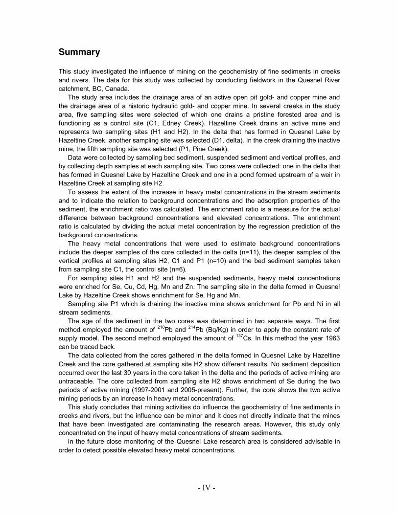
4.1.1 Particle size distribution Differences in particle size distribution were observed for all of the sampling sites. Sampling sites H2 and C1 show comparable distributions with a 90% contribution of  small  grain  sizes  (<60  μm).   Sampling sites H1  and  D1  are  comparable  as  well  and  show  85%  contribution  of  the  fraction  <60  μm.  The same applies to sampling site P1, but this site shows a smaller contribution of the fraction 60-240 μm  which  indicates  that more coarse material is available (figure 4.1).

Figure 4.1 Mean particle size distributions for sampling sites H1, H2, C1, D1 and P1.

- 19 -

4.1.2 Concentration of stored sediments No obvious patterns are observed in the concentration of stored sediment per sampling site (table 4.1).

Table 4.1 Average concentrations of gravel stored sediments per sampling site.

Sampling Site Average stored sediment concentration (g/m2)

H1 116,28 H2 388,99 C1 261,72 D1 773,53 P1 231,47

4.1.3 Organic matter content The largest organic matter (OM) content is observed at sampling site H1. Sampling sites H1 and H2 show OM percentages that are a factor 2 larger as sampling sites C1 and D1. Sampling site P1 has the lowest OM content (table 4.2). The low OM content at sampling site P1 is probably caused by the little amount of vegetation in that area. Table 4.2 Sampling sites and their average organic matter content.

Sampling Site Average organic matter content (%)

H1 31.63 H2 24.42 C1 15.36 D1 16.21 P1 3.47

- 20 -

4.2 Heavy metal concentrations

4.2.1 Quesnel Lake research area The heavy metal concentrations in the Quesnel Lake research area show different values per sampling site. Both the control site (C1) and the delta site (D1) show the lowest heavy metal concentrations. The heavy metal concentrations of these sampling sites lie close together.

For Al, Se, Cu, and Hg sampling sites H1 and H2 contain the highest concentrations. The Al concentration at sampling site H2 are largest for both the BS and the sediment core (figure 4.2 – 4.5), (the description of figure 4.2 applies for figures 4.3 – 4.6).

The Se concentrations of the SS at sampling site H1 are five times as high as sampling sites C1 and D1. The Se concentration in the BS of sampling site H1 is twice as high as for the control site and D1. The deeper sample at sampling site H1 has comparable concentrations as sampling sites C1 and D1. The concentrations in the BS and the SS of sampling site H2 are also twice as high as the control site and sampling site D1. The deeper samples show average concentrations (figure 4.3).

For Cu, the concentrations at sampling sites H1 and H2 are twice as high as sampling sites C1 and D1. The deeper samples at sampling sites H1 and H2 show smaller Cu concentrations (figure 4.4).

The Hg concentrations are not as elevated as Cu concentrations, however, sampling sites H1 and H2 show elevated concentrations (figure 4.5).

The heavy metal concentrations of As and Fe deviate from the above described pattern. Sampling sites C1 and D1 contain higher concentrations of As and Fe compared to the other sampling sites. The deeper samples taken at the sampling site C1 contain the highest concentrations (figures 4.6 and 4.7).

The elevated Fe and As concentrations at these sampling sites can be explained by a natural processes. Arsenic can be fractionated in different forms, including Fe-arsenate (Adriano, 2001). Arsenic is also likely to adsorb to Fe-hydroxides (Van der Perk, 2006). Iron is a transition metal and, after  Al,  the  second  most  abundant  metallic  element  in  the  earth’s  crust.  Further, after weathering, Fe precipitates relatively fast (Van der Perk, 2006). At sampling site C1, the weathered Fe has probably precipitated with As causing the elevated concentrations.

- 21 -

Figure 4.2 Al concentrations per sampling site and category. (The Boxplot shows the median value (line in the middle), the bottom box showing the 25% percentile, the top box showing the 75% percentile, the bottom line (dotted) showing the lowest concentration and the top line (dotted) showing the highest concentrations. The separate dots show the outliers. The number of samples per class: C1BS, H1BS, H2BS and – n=6, P1BS –n= 4, D1BS – n=2, H1 SS- n=2, H2SS – n=1, PC - n=9, D1C – n=20, H2C – n=20, P1SS – n=2, H1D - n=1, C1C – n=4).

Figure 4.3 Se concentrations per sampling site and category.

- 22 -

Figure 4.4 Cu concentrations per sampling site and category.

Figure 4.5 Hg concentrations per sampling site and category.

- 23 -

Figure 4.6 As concentrations per sampling site and category.

Figure 4.7 Fe concentrations per sampling site and category.

- 24 -

4.2.2 Cariboo Lake research area The most obvious observation for the Cariboo Lake research area is that this site has the lowest heavy metal concentrations, except for Pb (figure 4.8). Further, sampling site P1 contains elevated concentrations for Pb, Ce, Hf, La, Th and Zr.

Figure 4.8 Pb concentrations per sampling site and category.

The Pb concentrations in the vertical profile of sampling site P1 are relatively high. The Pb concentrations in the BS and SS samples are about two times as low as the depth profile samples, but they are elevated compared to the Pb concentrations at the sampling sites of the Quesnel Lake research area.

Secondary, the boxplots show higher concentrations for bismuth (Bi), cerium (Ce), hafnium (Hf), labthanum (La), thorium (Th) and zirconium (Zr) (appendix 2). Sampling site P1 does not show further elevations (for all metal concentration box-plots see appendix 2).

Bi is a by product in Pb, Tin (Sn) and Cu mining, it is thought to be the least toxic heavy metal, although it resembles Pb. The reason for the occurrence of high Bi concentrations at sampling site P1 is the copper- and gold mining that occurred in that area.

Th, Ce, La and Zr are common in the minerals monazite and zircon. Monazite is often found in placer deposits (Van Emden et al., 1997). Zircon occurs in sedimentary rock and is a major constituent of sand. Hf usually occurs together with Zircon (Mineral Data, 2001).

Ce, Hf, La, Th and Zr occur in high concentrations because of the placer deposits that can be found in the Cariboo Lake research area and the high concentration of sand in the bed material at sampling site P1 (figure 4.1).

Besides the differences in heavy metal concentrations between the sampling sites, differences in BS and SS occur as well. The box-plots show that for the Cariboo Lake research area, all heavy metal concentrations in the SS are lower than the heavy metal concentrations in the BS. In contrary, in the Quesnel Lake research area heavy metal concentrations in the SS show higher concentrations for Cu, Hg, and Se than concentrations of the BS.

- 25 -

4.3 Statistical analysis

In general, the metal enrichment in sediment differs between the Quesnel Lake research area and the Cariboo Lake research area. Sampling sites in the Quesnel Lake research area show elevated concentrations for the following metals: Se, Cu, Cd, Hg, Mn and Zn, whereas the Cariboo Lake sites show elevated concentrations only for Pb and Ni.

In this chapter, the correlation coefficients (R2) for the heavy metals with Al are given per sampling site, as are the p-value of the regression, the average and the S.E.. Further, the ER of these heavy metals are calculated.

Enrichment Factor Al - Se

y = 0.6696x + 0.08950

1

2

3

4

5

6

7

8

9

10

0 0.5 1 1.5 2 2.5Al (ppm)

Se (p

pm)

Reference Values

BS H1

BS H2

BS P1

BS D1

BS C1

SS

SS P1

Vertical Profile P1

S.E.

Linear (Reference Values)

Figure 4.9 Se: Al plotted for the reference values, the control site C1, bed- and SS for sampling site H1 and H2 and the BS for sampling site P1.

Table 4.3 Statistical parameters of the regression prediction for Se.

regression prediction Se y = 0.06696x+0.0895 p-value regression 1.69*10-6

Average Background concentrations (ppm) 1.06

Standard Error (ppm) 0.20

R2 0.59 Figure 4.9 shows the relationship between Se and Al. Sampling sites H1 and H2, for the BS and the SS vary considerably from the background concentrations. The regression of the background concentrations between Se and Al is significant (p-value < α,  α  =  0.05,  table 4.3).

The ER for the BS at sampling site H1 (ERbsH1) amounts 4.59. The ER for the BS at sampling site H2 (ERbsH2) is 3.24. The ER for the BS at sampling site D1 (ERbsD1) is 1.98 and the ER for the SS at sampling sites H1 and H2 (ERss) is 6.98. This indicates that enrichment of Se occurs on those sites and that the Se enrichment of the SS is higher compared to that of the BS.

Se concentrations show a high ER in the sediments of Hazeltine Creek. The active open pit gold- and copper mine which Hazeltine Creek is draining is located in a geological unit (Nicola Group) containing volcanic basaltic rock (see ch.2.2 Local Geology). These volcanic basaltic rocks contain large amounts of sulphur-deposits (Alloway, 1995). In the environment, Se is generally associated with

- 26 -

sulphur and it is found in metal-sulphur deposits (Conde and Sanz Alaejos (1997), Adriano (2001)) such as Silver (Au), Cu, Pb, Hg or other metals (Adriano (2001), Fishbein (1983)).

Therefore, it can be assumed that the mine is the main source of Se enrichment in the Quesnel Lake research area. Due to mining activities, more source rock is exposed to erosion which probably causes increased weathering of the rock, and thus a higher release of heavy metals to the environment.

It is remarkable that even though sampling site D1 is also part of Hazeltine Creek, no elevated concentrations occur at this sampling site.

Enrichment Factor Al - Cu

y = 7.6007x + 34.458

0

20

40

60

80

100

120

0 0.5 1 1.5 2 2.5Al (ppm)

Cu (p

pm)

Reference Values

BS H1

BS H2

BS P1

BS D1

BS C1

SS

SS P1

Vertical Profile P1

S.E.

Linear (Reference Values)

Figure 4.10 Cu: Al plotted for the reference values, the control site C1, BS and SS for sampling sites H1 and H2 and the BS for site P1. Table 4.4 Statistical parameters of the regression prediction for Cu.

regression prediction Cu y = 7.6007x+34.468 p-value regression 0.15

Average Background concentrations (ppm) 45.56

Standard Error (ppm) 9.36

R2 0.08 Figure 4.10 shows that the Cu concentrations in BS and SS of sampling sites H1 and H2 are elevated compared to the background concentrations.

Table 4.4 shows that the regression is not significant (p-value > α).   If the samples of the Cariboo Lake research area are left out of the background concentrations (circled in figure 4.10), the regression becomes significant (p-value   <   α,   appendix   3). This indicates that a difference in background concentrations exists between the two research areas. The differences in geology of the two research areas might cause the differences in background metal concentrations.

Because of the insignificant relation with Al, the ER could have been compared to the average of the background concentrations instead of the regression prediction. However, in order to remain consistency in the data analysis, the was calculated from the regression prediction for copper including the Cariboo Lake samples. If insignificant regressions occurred for the other heavy metals in this analysis, the ER was also calculated from regression prediction.

- 27 -

The ERbsH1 is 2.06, the ERbsH2 is 2.07 and the ERss is 2.31. This indicates that the Cu concentrations are enriched for sampling sites H1 and H2 in the BS and SS. The SS are slightly more enriched compared to the BS. Sampling site D1 is not enriched with copper (ERbsD1 is 1.05).

As was mentioned earlier, background copper concentrations can be substantial in basic igneous rocks. Further, according to the porphyry deposits of the Canadian Cordillera the soil around the active gold- and copper mine contains more than 200 ppm Cu (Gillstorm, 2004). Therefore, the copper enrichment of H1, H2 and the SS are probably also caused by the fact that mining activities are exposing large amounts of rocks to erosion which contain substantial amounts of copper.

Enrichment Factor Al - Cd

y = 0.1074x + 0.1439

0

0.1

0.2

0.3

0.4

0.5

0.6

0 0.5 1 1.5 2 2.5Al (ppm)

Cd (p

pm)

Reference Values

BS H1

BS H2

BS P1

BS D1

BS C1

SS

SS P1

Vertical Profile P1

S.E.

Linear (Reference Values)

Figure 4.11 Cd: Al plotted for the reference values, the control site, bed- and SS for sampling sites H1 and H2 and the BS for sampling site P1. Table 4.5 Statistical parameters of the regression prediction for Cd.

regression prediction Cd y = 0.1074x+0.1439 p-value regression 0.035

Average Background concentrations (ppm) 0.30

Standard Error 0.09

R2 0.16 Figure 4.11 shows that the Cd concentrations in BS and SS at sampling sites H1 and H2 and the BS at sampling site C1 are elevated compared to the background concentrations. Table 4.5 shows that the regression is significant (p-value < α). The ERbsH1 is 1.47, the ERbsH2 is 1.26 and the ERss is 1.60.

Probably the Cd concentrations in the BS of the Quesnel Lake research area are slightly increased compared to the deeper samples because of the fact that Cd is present in copper ores (Van der Perk, 2006). Therefore, the elevated concentrations are probably caused by erosion of the source rock. Because of the fact that the Cd concentrations of sampling site C1 and the sampling sites in Hazeltine Creek show a close resemblance, the enrichment of Cd probably only has a minor relation to mining activities.

- 28 -

Enrichment Factor Al - Hg

y = 0.0879x - 0.0571

-0.05

0

0.05

0.1

0.15

0.2

0 0.5 1 1.5 2 2.5

Al (ppm)

Hg (p

pm)

Reference Values

BS H1

BS H2

BS P1

BS D1

BS C1

SS

SS P1

Vertical Profile P1

S.E.

Linear (Reference Values)

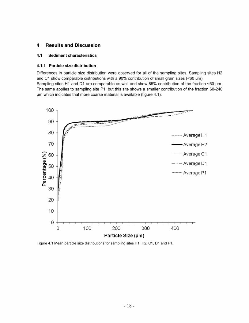
Figure 4.12 Hg: Al plotted for the reference values, the control site, bed- and SS for sampling sites H1 and H2 and the BS for sampling site P1. Table 4.6 Statistical parameters of the regression prediction for Hg.

regression prediction Hg y = 0.0879x - 0.0571 p-value regression 4.06*10-11

Average Background concentrations (ppm) 0.074

Standard Error (ppm) 0.015

R2 0.81 Figure 4.12 shows that the Hg concentrations are elevated for both the BS at sampling site H1 and the SS sediments. The p-value of the regression of the background concentrations is significant (p-value  <  α,  table  4.6).  The  ERbsH1 is 1.54, ERss is 1.98.

The reason for the Hg concentrations to be enriched for the sampling sites H1 and the SS draining the active mine  is  probably  caused  by  the  fact  that  Hg  occurs  in  the  earth’s  crust  mainly  as  sulphide  (Adriano, 2001), which indicates that that the Hg is derived from the source rock of the mine.

The fact that sediments retain Hg as Organic Matter (OM) complexes, on sorption sites of clays or as accumulating particles (Adriano, 2001) might be the explanation for the Hg concentrations to be higher at sampling site H1 compared to sampling site H2. Despite the fact that these sampling sites are located in the same creek, the OM concentrations at sampling site H1 are higher compared to sampling site H2 (table 4.2).

Here again location D1 does not show elevated concentrations.

- 29 -

Enrichment Factor Al - Mn

y = -37.717x + 753.49

0

1000

2000

3000

4000

5000

6000

7000

0 0.5 1 1.5 2 2.5Al (ppm)

Mn

(ppm

)

Reference Values

BS H1

BS H2

BS P1

BS D1

BS C1

SS

SS P1

Vertical Profile P1

S.E.

Linear (ReferenceValues)

Figure 4.13 Mn: Al plotted for the reference values, the control site, bed- and SS for sampling sites H1 and H2 and the BS for sampling site P1

Table 4.7 Statistical parameters of the regression prediction for Mn.

regression prediction Mn y = -37.717x+ 753.49 p-value regression 0.87

Average Background concentrations (ppm) 697.34

Standard Error (ppm) 405.88

R2 0.001

Figure 4.13 shows that regression of Mn and Al for the background concentrations. The regression is not significant (p-value > α,  table  4.7)  which  indicates  that  the  Mn  is  not  related  to  Al  en  therefore  clay  content. The ERbsH1 is 3.55, the ERbsH2 is 6.14, the ERbsD1 is 2.39 and the ERss is 5.92.

Although the ER are high, the relation that is shown in the background concentrations is not significant, the correlation of Mn with Al is small as well and the S.E. is relatively high (table 4.7). This indicates that the ER of Mn is neither related to background concentrations, clay content or mining activities. This is confirmed by the fact that Mn is one of the most abundant metal in soils (as are Al and Fe) (Lenntech, 2009) and is therefore probably not related to anthropogenic inputs.

- 30 -

Enrichment Factor Al - Zn

y = 13.155x + 64.59

0

50

100

150

200

250

0 0.5 1 1.5 2 2.5Al (ppm)

Zn (p

pm)

Reference Values

BS H1

BS H2

BS P1

BS D1

BS C1

SS

SS P1

SS Vertical Profile

E.R.

Linear (Reference Values)

Figure 4.14 Zn: Al plotted for the reference values, the control site, bed- and SS for sampling sites H1 and H2 and the BS for sampling site P1. Table 4.8 Statistical parameters of the regression prediction for Zn.

regression prediction Zn y = 13.155x+ 64.59 p-value regression 0.21

Average Background concentrations (ppm) 84.17

Standard Error (ppm) 18.88

R2 0.06 Figure 4.14 shows that Zn concentrations are elevated for the BS at sampling site H1 and the Zn concentrations of sampling site C1 are higher than the S.E. of the regression. Further the concentrations lie close together. The regression prediction of the background concentrations is not significant (p-value   >   α,   table 4.8). However, if the samples of the Cariboo Lake research area are excluded from the background concentrations (circled in figure 4.14), the regression prediction becomes significant (p-value   <   α, appendix 3). This indicates that, as was the case for copper, a difference exists between the background concentrations of the two research areas.

The ERbsH1 is 1.78, the ERbsH2 is 1.26 and the ERss is 1.34. Zinc concentrations might be elevated because of the fact that Zn is found in metalliferous ores as zinc-sulphide (Van der Perk, 2006). Therefore the elevated concentrations that are shown can probably be contributed to weathering of the source rock. Because of the fact that the Zn concentrations of sampling site C1 and the sampling sites in Hazeltine Creek show a close resemblance, the enrichment of Zn probably only has a minor relation to mining activities.

- 31 -

Enrichment Factor Al - Pb

y = -11.881x + 29.328

0

5

10

15

20

25

30

35

40

45

0 0.5 1 1.5 2 2.5Al (ppm)

Pb (p

pm)

Reference Values

BS H1

BS H2

BS P1

BS C1

BS D1

SS

Lineair (Reference Values)

Figure 4.15 Pb: Al plotted for the reference values, the control site, bed- and SS for sampling sites H1, H2 and the bed sediment samples for sampling site P1.

Enrichment Factor Al - Pb

y = 1.5547x + 6.5089

0

10

20

30

40

50

60

70

80

90

0 0.5 1 1.5 2 2.5Al (ppm)

Pb (p

pm)

Reference Values

BS H1

BS H2

BS P1

BS C1

BS D1

SS

SS P1

Vertical Profile P1

E.R.

Linear (Reference Values)

Figure 4.16 Pb: Al plotted for the reference values, the control site, bed- and SS for sampling sites H1 and H2, the BS for sampling site P1 and the vertical profile at sampling site P1.

Table 4.9 Statistical parameters of the regression prediction for Pb.

regression prediction Pb y = 1.5547+ 6.5089 p-value regression 0.43

Average Background concentrations (ppm) 8.99 Standard Error (ppm) 2.12

R2 0.027

- 32 -

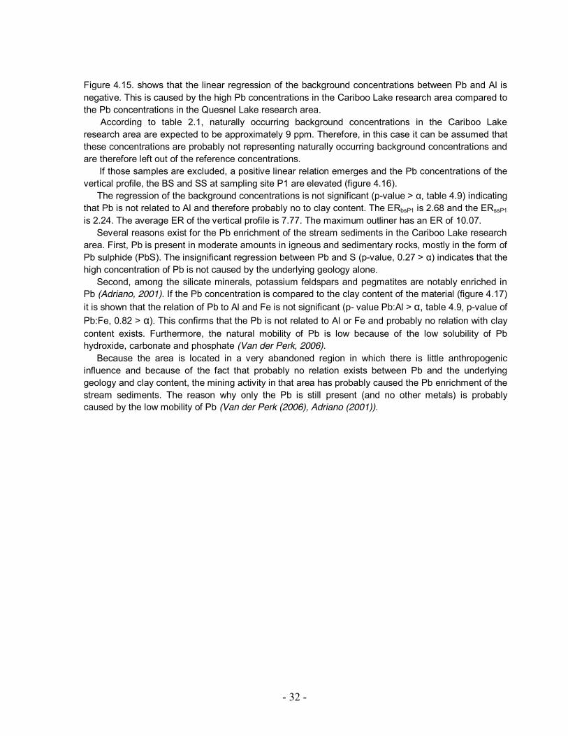
Figure 4.15. shows that the linear regression of the background concentrations between Pb and Al is negative. This is caused by the high Pb concentrations in the Cariboo Lake research area compared to the Pb concentrations in the Quesnel Lake research area.

According to table 2.1, naturally occurring background concentrations in the Cariboo Lake research area are expected to be approximately 9 ppm. Therefore, in this case it can be assumed that these concentrations are probably not representing naturally occurring background concentrations and are therefore left out of the reference concentrations.

If those samples are excluded, a positive linear relation emerges and the Pb concentrations of the vertical profile, the BS and SS at sampling site P1 are elevated (figure 4.16).

The regression of the background concentrations is not significant (p-value > α,  table  4.9) indicating that Pb is not related to Al and therefore probably no to clay content. The ERbsP1 is 2.68 and the ERssP1 is 2.24. The average ER of the vertical profile is 7.77. The maximum outliner has an ER of 10.07.

Several reasons exist for the Pb enrichment of the stream sediments in the Cariboo Lake research area. First, Pb is present in moderate amounts in igneous and sedimentary rocks, mostly in the form of Pb sulphide (PbS). The insignificant regression between Pb and S (p-value, 0.27 >  α)  indicates that the high concentration of Pb is not caused by the underlying geology alone.

Second, among the silicate minerals, potassium feldspars and pegmatites are notably enriched in Pb (Adriano, 2001). If the Pb concentration is compared to the clay content of the material (figure 4.17) it is shown that the relation of Pb to Al and Fe is not significant (p- value Pb:Al > α,  table 4.9, p-value of Pb:Fe, 0.82 > α). This confirms that the Pb is not related to Al or Fe and probably no relation with clay content exists. Furthermore, the natural mobility of Pb is low because of the low solubility of Pb hydroxide, carbonate and phosphate (Van der Perk, 2006).

Because the area is located in a very abandoned region in which there is little anthropogenic influence and because of the fact that probably no relation exists between Pb and the underlying geology and clay content, the mining activity in that area has probably caused the Pb enrichment of the stream sediments. The reason why only the Pb is still present (and no other metals) is probably caused by the low mobility of Pb (Van der Perk (2006), Adriano (2001)).

- 33 -

Pb: Al/Fe

y = -63.153x + 85.391R2 = 0.1259

y = 5.4157x + 17.597R2 = 0.004

0

10

20

30

40

50

60

70

80

90

0 1 2 3 4Al/Fe (ppm)

Pb (p

pm)

Pb:Al

Pb:Fe

Figure 4.17 Pb plotted against Al and Fe for sampling site P1.

Enrichment Factor Al - Ni

y = 5.7913x + 20.986

0

5

10

15

20

25

30

35

40

45

0 0.5 1 1.5 2 2.5Al (ppm)

Ni (p

pm)

Reference Values

BS H1

BS H2

BS P1

BS D1

BS C1

SS

SS P1

Vertical Profile P1

E.R.

Linear (Reference Values)

Figure 4.18 Ni: Al plotted for the reference values, the control site, bed- and SS for sampling sites H1 and H2, the BS for sampling site P1 and the vertical profile at sampling site P1.

- 34 -

Table 4.10 Statistical parameters of the regression prediction for Ni. regression prediction Ni y = 5.7913x + 20.986

p-value regression 0.22

Average Background concentrations (ppm) 30.24 Standard Error (ppm) 5.09

R2 0.06 Figure 4.18 shows that the Ni concentrations in BS and SS at sampling site P1 are elevated. The

regression of the background concentrations is not significant. Therefore Ni can not be related to Al and therefore probably not to clay content. The ER of the BS at sampling site P1 is 1.25, for the SS it is 1.19 and for the vertical profile it is 1.28. This indicates that the Cariboo Lake research area is slightly enriched with Ni. Summarizing, sampling sites H1, H2 and D1 are enriched in Se, Hg and Mn. Sampling sites H1 and H2 are enriched in Cu, Cd and Zn. Sampling site P1 is enriched in Pb and Ni for all stream sediments (table 4.11).

The enrichment of Se, Cu and Hg is probably caused by the fact that mining activities are exposing large amounts of rocks to erosion. The enrichment of Cd and Zn only seem to have a minor relation to mining activities because of the fact that the BS of the sampling site C1 shows comparable metal concentrations as the BS and SS of sampling sites H1, H2 and D1.

In the Cariboo Lake research area, the enrichment of Pb and Ni is probably caused by historic mining activities. In the Quesnel Lake research area the concentrations of Se, Cu, Cd and Hg are higher in the SS than in the BS. In the Cariboo Lake research area, the SS show lower Pb and Ni concentrations compared to the BS and the vertical profile. The differences that occur in heavy metal background concentrations are probably caused by the underlying geology of the two research areas.

Table 4.11 ER for Se, Cu, Hg, Mn, Zn, Pb and Ni for every sampling site.

Sampling Site

Se Cu Cd Hg Mn Zn Pb Ni

BS H1 4.23 2.06 1.47 1.54 3.55 1.78 0.92 0.90 BS H2 2.98 2.07 1.26 1.25 6.14 1.26 0.80 0.76

BS P1 1.04 0.87 1.14 0.62 1.04 1.36 2.68 1.25

BS D1 1.82 1.05 1.17 1.41 2.39 1.03 0.83 0.96

SS 6.43 2.31 1.60 1.98 5.92 1.34 0.86 0.89

SS P1 0.97 0.73 1.02 1.62 0.84 0.97 2.24 1.19 Vertical

Profile P1 0.53 1.19 0.82 0.18 1.01 1.00 5.16 1.28

4.3.1 Low concentrations bed sediments at sampling site D1 Although the BS at sampling sites H1 and H2 show enrichment for Se and Cu, no enrichment occurs at sampling site D1. This can be caused by the fact that Hazeltine Creek confluences with Edney Creek and the heavy metal concentrations are diluted. However, then it would be expected that heavy metal concentrations were elevated compared to sampling site C1, which is not the case. Sediments could be settling in Hazeltine Creek somewhere upstream of the confluence with Edney Creek.

Besides this, the delta is very dynamic, and BS are deposited over a larger area than the sampled stream. This was already shown by the low deposition rates in the first centimetre of the core taken at sampling site D1.

- 35 -

4.3.2 Bed sediment compared to suspended sediment Table 4.11 shows that the enrichment with Se, Cu, Cd and Hg of the SS is higher than the enrichment in the BS for sampling sites H1 and H2. This implies that the sediment that is transported contains higher heavy metal concentrations compared to the sediment that is already deposited. At the moment the SS settles, the heavy metal enrichment of the bed sediment will increase. At sampling site P1, the opposite occurs: the ER for the SS are lower compared to the BS. Thus, the enrichment of the BS will decrease at the moment SS is deposited.

4.3.3 Comparison with background concentrations Table 4.12 shows the background concentrations per geological unit and per sampling site. Here it can be observed that the metals with the high ER show higher concentrations compared to background concentrations.

For sampling sites H1, H2 and the SS these are Se, Cu, Cd, Hg, Mn and Zn. At sampling site P1 this is only valid for Pb. For a detailed comparison with the naturally occurring background values and underlying geology be referred to the other part of this research (Karimlou, (2011)).

Table 4.12 Heavy metal background concentrations per geological unit compared to the heavy metal concentrations per sampling site. Metal (ppm)

Snowshoe group

(uPrPzSn)

Calc-alkaline volcanic

rock (EKaca)

Basaltic volcanic

rocks (uTrNvb)

BS C1 BS H1 BS H2 BS D1 BS P1 SS SS P1

As 3.18 2.12 7.74 1.58 1.73 1.90 1,38 0.93 1.57 0.72 Cd 0.26 0.19 0.3 0.44 0.48 0.44 0.34 0.28 0.50 0.23 Cu 20.91 18.77 38.2 41.98 97.87 101.25 47.25 36.15 106.93 29.05 Fe 2.26 2.74 1.82 3.27 3.01 2.72 2.84 3.27 2.47 2.79

Hg (ppb) 34.68 55 62.82 81.67 146.67 136.67 90.00 15.00 160.00 10.00 Mn 500.91 320 1062.82 1300 2440 4187 1675 750 4110 608 Pb 9.52 5.39 5.7 8.87 8.43 7.53 7.15 21.33 7.67 17.10 Se 0.5 0.28 0.59 1.33 5.73 4.40 2.00 0.80 7.97 0.60 Zn 62.32 40.71 54.52 111.00 155.83 113.17 85.50 104.50 114.33 71.50

- 36 -

4.4 Age of the sediment cores 4.4.1 Lead – 210

Figure 4.19 Pb210 and Pb214 depth profile for the core collected at sampling site D1, leaving out the first cm of zero sediment deposition.

As mentioned before, the first cm of the core collected at sampling site D1 was not sampled. Besides the missing first centimetre, during analysis it became obvious that the total amount of 210Pbu was higher at sampling site H2 compared to sampling site D1. According to Appleby et al. (1983) the total 210Pbu should compare in cores collected in the same catchment. Therefore, it was assumed that this first centimeter of the core represented a period of zero sediment deposition containing the missing amount of 210Pbu.

In order to calculate the age of the sediments in the core collected at sampling site D1, the total amount of 210Pbu has to be known. The total amount of 210Pbu in the core collected at sampling site D1 is assumed to be equal to the total amount of 210Pbu in the core collected at sampling site H2.

The total amount of 210Pbu at sampling site H2 to a depth of 1 m amounted approximately 40,000 Bq/m2. The total amount of 210Pbu at sampling site D1 to a depth of 1 m amounted 16,000 Bq/m2. This indicates that the amount of approximately 24,000 Bq/m2 210Pbu was missing in the core collected at sampling site D1. Thus in the following analysis, the first centimeter of the core collected at sampling site D1 is assumed to contain approximately 24,000 Bq/m2 210Pbu, which corresponds with approximately 1432 Bq/kg. The amount of 214Pb was assumed to remain relatively constant throughout the core and was set at 46.00 Bq/kg in the first centimeter.

In the core collected at sampling site D1, the 210Pb concentrations decrease rapidly in the first cm. After that, from 1 – 4 cm it decreases further, but less rapid. A slight increase over the section 4 - 5 cm can be observed, in the section 5 - 6 cm the concentration decreases again and then in the section 6 - 8 cm the highest 210Pb value in the entire core is observed (figure 4.19). Further down the core, in the section 15 - 19 cm, another high 210Pb value is observed. The same differences can be observed for

Depth (cm)

210-Pb (Bq/kg)

214-Pb (Bq/kg)

1 1432.31 46.00 2 85.24 46.58 3 79.47 46.58 4 80.68 44.96 5 75.79 42.03 6 88.06 45.55 7 66.27 45.03 8 91.88 54.49 11 71.35 42.73 12 78.59 46.56 13 67.82 42.21 14 68.66 42.68 15 61.85 45.05 16 74.83 46.42 20 82.18 61.99 27 52.29 45.06 37 62.26 40.04 42 51.92 52.8 44 61.75 46.27

1

6

11

16

21

26

31

36

41

46

51

0 20 40 60 80 100

Pb-210/Pb-214 (Bq/Kg))

Dep

th (c

m)

Pb-210

Pb-214

- 37 -

the 214Pb concentrations. Those are relatively constant with elevated values in the 6 - 8 cm section and the 15 - 19 cm section. Deeper down the core the 210Pb concentrations approach the 214Pb concentrations.

By applying the exponential function that can be calculated for the 210Pbu the extrapolation approaches the asymptote at 70 cm depth (figure 4.20 and 4.21). After applying the CRS model, the age of the sediments can be predicted. From figure 4.22 it becomes obvious that an age of 47 year (1963) agrees with a depth of 13 cm.

Figure 4.20 Pb-210 U with the exponential prediction included, the first cm of zero deposition is included which gives a distorted view.

Figure 4.21 Pb-210 U extrapolation, minus the first cm to optimize the depiction of the relation given in figure 4.20.

Figure 4.22 Age prediction of the sediments in the core collected at sampling site D1.

- 38 -

0

2

4

6

8

10

12

14

16

18

20

0 50 100 150 200

Pb-210/Pb-214 (Bq/Kg))

Dep

th (c

m)

Pb-210

Pb-214

Figure 4.23 Depth profile for the core collected at sampling site H2.

In the core collected at sampling site H2, the 210Pb concentrations decrease in the first 5 cm. In the section 5 - 6.5 cm the highest 210Pb value in the entire core is observed (figure 4.23). Further down the core between 12 and 14 cm, another high 210Pb is observed. In contrast with the core collected at sampling site D1, the 214Pb values are relatively constant in this core. In this core, the effect of the 210Pb approaching the 214Pb concentration is more obvious than in the other core. The next few figures show the 210Pbu extrapolation and the time-depth profile for the core collected at sampling site H2. The same method was applied as was for the core collected at sampling site D1 (figures 4.24 and 4.25).

Figure 4.26 shows that the depth-age predictions do not compare. This is caused by the fact that during the last 26 years no sediment deposition occurred in the core collected at sampling site D1. The slope of the linear prediction show a close resemblance. Therefore, the sediment accumulation rates are closely related for the two cores.

Depth Pb-210 (Bq/Kg)

Pb-214 (Bq/Kg)

1 125.5 25.98

3 119.3 24.12

5 115.4 22.43

6,5 150.9 28.03

7,5 123.6 24.83

8,5 110.6 23.88

10 104.8 30.53

12 85.5 29.08

14 121.3 32.9

16 74 27.1

19 69.6 24.5

- 39 -

Figure 4.24 Pb-210 U extrapolation.

Figure 4.25 Age prediction of the sediments in the core collected at sampling site H2.

Figure 4.26 Age predictions for cores collected at sampling site D1 and H2.

- 40 -

4.4.2 Caesium-137

0

5

10

15

20

25

30

35

40

45

50

0 5 10 15 20

Cs-137 (Bq/Kg)

Dep

th (c

m)

D1

Figure 4.27 Cs137 depth profile for the core collected at sampling site D1.

0

2

4

6

8

10

12

14

16

18

20

40 50 60 70 80 90

Cs-137 (Bq/Kg)

Dep

th (c

m)

Figure 4.28 Cs137 depth profile for the core collected at sampling site H2.

Depth (cm)

Cs-137 (Bq/kg)

2-sigma

1 15,4 5,01 2 9,89 3,38 3 10,93 3,08 4 9,61 3,09 5 7,4 2,43 6 10,32 3,25 8 13,81 4,65

10 12,2 3,39 11 11,99 4,13 12 9,33 1,98 13 8,95 1,92 14 8,38 1,53 15 17,65 4,59 19 6,79 2,19 26 0 3 36 0 2,59 41 0 1,96 43 0 2,19 46 0 4,15

Depth (cm)

Cs-137 (Bq/kg)

2-sigma

1 54.36 5.85

3 66.09 6.05

5 71.49 6.67 6.5 69.32 5.61 7.5 68.72 6.01 8.5 80.32 6.63 10 69.71 5.47 12 66.76 5.67 14 82.92 8.96

16 74.56 6.12

19 65.3 6.61

- 41 -

In the core collected at sampling site D1, the 137Cs concentration is high in the first centimeter, but it decreases going downward. The large peak at the 14-15 cm increment is obvious. After that the 137Cs concentration decreases towards zero (figure 4.27).

According to the 137Cs dating, the year 1963 corresponds to a depth of 14-15 cm. For the 210Pb dating, this year corresponds to a depth of 13 cm. This indicates that the dates do not correspond exactly, but addressing the uncertainty considering the first cm of the core, it can be assumed that the ages found in the core collected at sampling site D1 are reliable.

In the core collected at sampling site H2 the 137Cs values are much higher compared to the core collected at sampling site D1. The 137Cs concentration increases in the first 5 cm after which it decreases again. There are two peaks in this core: the first peak is at 8.5 cm depth and the second at 14 cm depth.

The 137Cs concentrations do not reach zero in the core collected at sampling site H2 (figure 4.27) therefore the year 1963 cannot be traced back. This indicates that the 137Cs dating of this core cannot accept or reject the dates found with the 210Pb dating method for the core collected at sampling site H2.

- 42 -

4.4.3 Heavy metal concentration profiles The gold- and copper mine in the Quesnel Lake research area was active from 1997-2001. According to the 210Pb dating of the core collected at sampling site H2 this age corresponds to a depth of approximately 8.5 cm – 5 cm. The start of the second mining period in the year 2005 is corresponds to a depth of approximately 4 cm. Thus, the ending of the first period and the beginning of the second period are situated very close together.

The two mining periods are untraceable in the core that was collected at sampling site D1.

Cu

02468

101214161820

0 20 40 60 80 100

Cu

Se

02468

101214161820

0 0.5 1 1.5 2 2.5 3

Se

Mn

02468

101214161820

0 200 400 600 800 1000 1200

Mn

As

02468

101214161820

0 2 4 6 8 10

As

Figure 4.29 Metal concentrations (horizontal axis, ppm) plotted against depth (vertical axis, cm) for the core collected at sampling site H2. The red shading indicates the period 1997-2001, the green shading indicates the period of 2005 - present. Figure 4.29 shows the first mining period (highlighted with red shading) and the second period (highlighted with green shading). The concentration of Cu in the sediment increases during the first mining period from 60 ppm to 70 ppm after which it decreases again. In between the two periods the Cu concentration stays constant around a concentration of 65 ppm. During the second mining period the Cu concentration increases even more up to 80 ppm in the surface layer.

The Se concentrations increase even more, almost a factor two. During the first mining period the concentrations increase from 1.5 ppm – 2 ppm. In between the two periods of active mining the Se concentration seems to diminish, but during the second period of active mining it increases to a concentration of 2.7 ppm in the surface layer.

For Mn, there is also an increase in the two mining periods, and a decrease in concentration in between the two periods (figure 4.29).

For As and Cd concentrations increase during the first period of active mining, however, the concentrations either stay constant or diminish during the current period of active mining (figure 4.29 and appendix 6).

- 43 -

Although As, Cu, Mn and Cd show an increase in their concentration, enrichment occurs for Se only. The mean ER of Se during the first period of active mining is 1.37 with a maximum value of 1.54 (figure 4.30). The mean ER of Se during the second period of active mining is 1.86 with a maximum value of 2.14 (figure 4.30).

Al:Se

y = 0.6696x + 0.0895

0

0.5

1

1.5

2

2.5

3

0 0.5 1 1.5 2 2.5

Al (ppm)

Se (p

pm)

Reference ValuesActive period 1 (1997-2001)Avtive period 2 (2005 - present)S.E.Linear (Reference Values)

Figure 4.30 Reference and core heavy metal concentrations for Se plotted against Al. From the above it becomes obvious that some of the metals show an increase in concentration during the first period of active mining, but they either stay constant or decrease during the second period of active mining.

During this second period of active mining, the mining cooperation has taken countermeasures to reduce contamination from their mining activities. During the first mining period, the mines tailings water were directed towards a tributary of Edney Creek and towards the mines drainage creek. Currently, the water is first directed trough an area were bio-remediation should decrease the toxicity of the water (Gillstrom (2004), Hitchcock (2009), presentation S. Baldwin, October 2010).

Another example of measures taken by the mining cooperation to reduce contamination is for example directing the surface runoff towards the tailings pond. Therefore less of the surface run-off inside of the mine will reach the outflow point in Hazeltine Creek. This can be traced back in core taken at sampling site H2 by the cease of increasing heavy metal concentrations.

- 44 -

5 Conclusions A field study to assess the effects of mining activities on the chemical composition of fine sediments in streams was conducted in the Quesnel River catchment, BC, Canada. For this purpose, a stream draining an active open pit gold- and copper mine (Hazeltine Creek) located in the Quesnel Lake research area and a stream draining a historic hydraulic gold- and copper mine (Pine Creek) located in Cariboo Lake research area were selected. In addition, a third stream (Edney Creek) located in the Quesnel Lake research area was selected to act as a control site. The heavy metal concentrations in suspended- and bed sediment were measured and the results of the three streams were compared.

Quesnel Lake research area and Cariboo Lake research area contain varying heavy metal concentrations. This is probably caused by the fact that the research areas have a different underlying geology. Further, differences are probably caused by the fact that in the Quesnel Lake research area the mine is still active whereas in the Cariboo Lake research area the mine is abandoned.

The bed- and suspended sediments of the two sampling sites H1 and H2 located in Hazeltine Creek draining the active open pit gold- and copper mine are enriched for Se, Cu, Cd, Hg, Mn and Zn. At sampling site D1, enrichment occurs for Se, Hg and Mn only.

At sampling site P1 in the Cariboo Lake research area enrichment for all stream sediments occurred for Pb and Ni.

The enrichment of Se, Cu and Hg in the Quesnel Lake research area is probably caused by the current mining activities. The enrichment of Pb and Ni is probably caused by the historic mining activities.

At sampling sites H1 and H2 it is shown that the suspended sediments contain higher heavy metal concentrations compared to the bed sediments. This implies that if the suspended sediments are deposited, heavy metal concentrations of the bed sediments will increase further. Therefore, the heavy metal concentrations of the bed sediments will probably increase in the future.

At sampling site P1, the enrichment of the suspended sediments is lower compared to the enrichment of the bed sediments. This implies that the enrichment of the bed sediments is decreasing. Therefore, the enrichment of the bed sediments will probably decrease in the future.

The periods of active mining could not be traced back in the core that was collected near sampling site D1. In the core collected at sampling site H2, the 210Pb dating showed that the two periods of active mining were present in the first 10 cm. The first period of active mining (1997-2001) corresponded to a depth of 8.5- 5 cm. The second period of active mining (2005 – present) corresponded to a depth of 4 cm- surface.

The concentrations of Se, Cu, Mn, As and Cd increased during the first period of active mining, but only for Se and Cu during the second period of active mining. Only enrichment of Se occurred in those two periods of active mining.

The lesser increase in heavy metal concentrations during the current mining period is probably caused by preventive measures that were taken by the mining cooperation. The heavy metal concentrations of the core collected at sampling site H2 confirm that the mine influences heavy metal concentrations in streambed sediments.

In this research, it is demonstrated that mining activities influence the geochemistry of the fine sediments in streams. Depending on the type of mine, the mining methods and the way the mine contains its tailings this influence can be minor or of a more substantial influence. The changing geochemistry is for a large part induced by the increased rock surface that is subject to weathering instead of anthropogenic input of those metals. Although this heavy metal input is due to anthropogenic activities, it probably has a natural origin.

Considering the metal enrichment of sediments in the stream draining the historic hydraulic gold- and copper mine that has been inactive for more than 80 years, it can be concluded that the influence

- 45 -

of mining activities on the surrounding environment can continue for a long period of time after the mining activities are halted.

In the future, monitoring of the Quesnel Lake research area is advised to detect possible elevated heavy metal concentrations in streams further downstream of the sites investigated in this study.

- 46 -

6 Acknowledgments First of all I want to thank my field partner Gosro Karimlou, without him it would not have been

possible to carry out this research. I would like to thank Marcel van der Perk from Utrecht University for his guidance and support before, during and after the fieldwork. Furthermore, I would like to thank Phil Owens and Ellen Petticrew from the University of Northern British Colombia for their guidance and support in Canada and for the opportunity to carry out the research at Quesnel River Research Centre. This brings us to the most valuable person for carrying out the fieldwork, Lazlo Enyedy. He almost had a part-time job in bringing us to our sampling sites. I want to thank him for this. In addition, I want to thank Richard Holmes for his hospitality and help during our research. I also want to thank Sam Albers and Alex Koiter for showing us around and helping us out with the LISST-ST and the filtering process. Finally, the use of the English language in the report was criticized by Floris Keizer and Sjoerd Theeuwen for which I would like to thank them.

The Molengraaf fund, the K.F.Hein fund and the ACSN provided us with the necessary funding; without their financial support the research would not have been possible.

- 47 -

7 References Ackerman E.A., (1941) The Köppen Classification of Climates in North America, Geographical

Review, Vol. 31, No.1, pp. 105-111 Adriano D.C., (2001) Trace Elements in Terrestrial Environments, Biochemistry, Bioavailability

and Risks of Metals, Springer, New York, 867p Alloway B.J., (1995) Heavy Metals in Soils, second edition, Blackie Academic & Professional,

London, New York, 368p ALS Group, Trace Level Methods Using Conventional ICP-AES Analysis, (last consulted 17-06-

2011).http://www.alsglobal.com/upload/minerals/downloads/methoddescriptions/Method%20Descriptions-ME-ICP41.pdf

Amos K.J., Croke J.C., Timmers H., Owens P.N., Thompson C., (2009) The application of caesium-137 measurements to investigate floodplain deposition in a large semi-arid catchment in Queensland, Australia: a low-fallout environment, Earth surface processes and landforms, 34, 515-529

Appleby P.G., Oldfield F. (1983) The Assessment of 210Pb data from sites with varying sediment accumulation rates, Hydrobiologica, 103, pp 29-35

Appleby P.G., Jones V.J., Ellis-Evans J.C., (1995) Radiometric dating of Lake sediments from Signy Island (maritime Antarctic): evidence of recent climate change, Journal of Paleolimnology, 13: 179-191, Kluwer Academic Publishers.

BeckerA., Klöck W., Friese K., Schreck P., Treutler H.C., Spettel B., Duff M.C., (2001) Lake Süsser See as a natural sink for heavy metals from copper mining, , Journal of Geochemical Exploration, 74, pp 205-217

Binford M.W., Kahl J.S., Norton S.A., (1993) Interpretation of 210-Pb profiles and verification of the CRS model in PIRLA project Lake sediment cores, Journal of Paleolimnology 9, 275-29

Canada Weather Office, National Climate Data and Information Archive, 2011, Daily report for June 1993, Likely, BC, (last accessed 17-06-2011) http://climate.weatheroffice.gc.ca/climateData/dailydata_e.html?timeframe=2&Prov=BC&StationID=607&dlyRange=1974-09-01|1993-12-31&Year=1993&Month=6&Day=01

Carter, J., Walling, D. E., Owens, P. N. & Leeks, G. J. L. (2006) Spatial and temporal variability in the concentration and speciation of metals in SS transported by the River Aire, Yorkshire, UK. Hydrol. Processes 20, 3007–3027

Conde J.E., Sanz Alaejos M., (1997) Selenium Concentrations in Natural and Environmental Waters, Chemical Reviews, 97, 1979-2003

Gillstorm G., (2004) Mount Polley Mine 2004 Feasibility Study, 43-101 Technical Report, Likely B.C. Canada, Imperial Metal Corporation Vancouver, B.C., Canada

Handbook of mineralogy, Zircon, Mineral Data Publishing version 1.2, (last accessed 02-11- 2011) http://rruff.geo.arizona.edu/doclib/hom/zircon.pdf

Helgen S.O., Moore J.N., (1996) Natural Background Determination and Impact Quantification in Trace Metal-Contaminated River Sediments, Environment Science Technology, 30, 129-135

Hitchcock  E.,  (2009)  ‘Mount  Polley  microbes  may  help  reduce  mine  waste’,  The  WilliamsLake   Tribune, December 3 2009.

Holland S.S., (1976) Landforms of British Colombia – A Physiographic outline, 1976, Bulletin 48, The Government of British Colombia

Hwang H-M., Green P.G., Holmes R.W., (2009) Antropogenic impacts on the qualtity of streambed sediments in the lower Sacramento River watershed, California, Journal of Environmental Science and Health Part A; 44, 1-11

Jackaman, W. (2008): QUEST Project sample reanalysis; Geoscience BC, Report 2008-3, 4 p.

- 48 -

Karimlou G., (2011) Effects of mining on fine sediment quality; a comparison with regional metal background concentrations, igitur archive, Utrecht University Krein, A., Petticrew, E., and Udelhoven, T., (2002) The use of fine sediment fractal dimensions

and colour to determine sediment sources in a small watershed. Catena 53, 165-179. Krishnaswami, S., D. Lal, J.M. Martin & M. Meybeck, (1971) Geochronology of Lake sediments.

Earth Planet. Sci. Lett., 11: 407-414. Lenntech (2009) Water Treatment Solutions, periodiek system der elementen, Mangaan, (last

accessed 9-11-2011) http://www.lenntech.nl/periodiek/elementen/mn.htm Loska K., Wiechula D., Pelczar J., (2011) Applications of Enrichment Factor to Assessment of

Zinc Enrichment/Depletion in Farming Soils, communications in Soil Science and Plant Analysis, 36, pp 1117-1128

Loring D.H., (1991) Normalization of heavy-metal data from estuarine and coastal sediments, CESJ, mar. Sci.,48: 101-115

Owens, P. N., Walling, D.E., (2002) The phosphorus content of fluvial sediment in rural and industrialized River basins. Water Research 36, 685-701.

Panteleyev, A., Bailey, D.G., Bloodgood, M.A., Hancock, K.D., (1996) Geology and mineral deposits map area, central Quesnel trough, British Colombia, Ministry of Employment and Investment, Energy and Mineral Division, Geological Survey Branch

Petticrew E.L., Krein A., Walling D.E. (2006) Evaluating fine sediment mobilization and storage in a gravel-bed River using controlled reservoir releases, Hydrological Processes, 21, 198-210

Pidwirny, M. (2006) "Climate Classification and Climatic Regions of the World". Fundamentals of Physical Geography, 2nd Edition. (last accessed 17-06-2011). http://www.physicalgeography.net/fundamentals/7v.html

Robbins J.A., (1975) Determination of recent sedimentation rates in Lake Michigan using Pb- 210 and Cs-137, Geochinica et Cosmochimica Acta, Vol. 39 pp. 285 to 304

Smith T.B., Owens P.N. (2010) Impact of land use activities on fine sediment associated contaminants, Quesnel River Basin, British Columbia, Canada, Sediment dynamics for a changing future (proceedings of the ICCE symposium held at The Warsaw University of Life Sciences-SGGW, Poland, 14-18 june 2010) IAHS Publ. 337, 2010

Soto-Jiménez M.F., Páez-Osuna F., (2000) Distribution and Normalization of Heavy Metal Concentrations in Mangrove and Lagoonal Sediments from Mazatlán Harbor (SE Gulf of California), Esuarine, Coastal and Shelf Science, 53, pp 259-274

Sutherland Brown A. (1976) Porphyry Deposits of the Canadian Cordillera, the Canadian institute of mining and metallurgy, special volume 15

Van der Perk M., (2006) Soil and Water contamination; from molecular to catchment scale, Taylor and Francis/Balkema, Leiden, 365p

Van Emden B., Thornber M.R., Graham J., Lincoln F.J. (1997) The incorporation of actinides in monazite and xenotime from placer deposits in western Australia, The canadian mineralogist, Vol 35. pp. 95-104

Walling D.E., HE Q., (1996) Rates of Overbank Sedimentation on the Floodplains of British Lowland Rivers Documented Using Fallout 137Cs, Geografiska Annaler, Vol. 78 A(4), pp 223-234

Walling D.E., HE Q., (1996a) Interpreting Particle Size Effects in the Adsorption of 137Cs and Unsupported 210Pb by Mineral Soils and Sediments, Journal Environmental Radiactivity, Vol. 30, No. 2, pp 117-137

Walling D.E., HE Q., (1997) The Distribution of Fallout 137Cs and 210Pb in Undisturbed and Cultivated Soils, Appl. Radiat. Ist., Vol. 48, No. 5, pp 677-690

- 49 -

Walling, D.E., Owens, P.N., Carter, J., Leeks, G.J.L., Lewis, S., Meharg, A.A., and Wright, J., (2003) Storage of sediment-associated nutrients and contaminants in river channel and floodplain systems. Applied Geochemistry, Volume 18, Issue 2, pp. 195-220.

Watson Burke E., (2008) Dating recent sedimentation rates in healthy marsh at Elkhorn Slough using Pb-210 and Cs-137 dating methods, Land, Air & Water Resources One Shields Ave. University of California, Davis Davis, CA 95616

Wooster J.K, Dusterhoff S.R., Cui Y., Sklar L.S., Dietrich W.E., Malko M. (2008) Sediment supply and relative size distribution effects on fine sediment infiltration into immobile gravels, Water Resources Research, Vol 44, wo 3424

- 50 -

Appendices Appendix 1 Correlations

Correlation of Se, Cu, Cd, Hg, Mn, Zb, Pb and Ni with Al for the separate sampling sites. The correlation is given in r. For BS D1 and SS P1 there were not enough samples to obtain a valid correlation. The SS at sampling sites H1 and H2 gave very high correlations which is probably due to the low amount of samples as well.

Sampling Site Number

of samples

Se Cu Cd Hg Mn Zn Pb Ni

BS H1 6 0.55 0.91 0.03 0.99 0.32 0.38 0.96 0.92 BS H2 6 0.73 0.85 0.84 0.80 0.60 0.73 0.76 0.96 BS D1 2 1 1 1 1 1 1 1 1 BS C1 6 0.64 0.19 0.16 0.13 0.77 0 0.63 0.63 BS P1 4 0.27 0.25 0.13 0.19 0 0.05 0.43 0.47

SS 3 0.95 0.99 0.99 0.41 0.99 0.98 0.99 0.13 SS P1 2 1 1 1 1 1 1 1 1 VP P1 9 0.79 0.55 0.72 0.10 0.33 0.86 0.17 0.76

VP H2 (0-9 cm) 9 0.28 0.45 0.60 0.26 0.21 0.39 0.25 0.47 VP H2 (9-

21cm) 5 0.33 0.35 0.89 0.23 0.82 0.97 0.91 0.99

VP D1 (0-8cm) 8 0.95 0.94 0.18 0.26 0.20 0.98 0.85 0.96 VPD1 (8-46cm) 12 0.80 0.91 0.71 0.94 0.51 0.97 0.95 0.98

Appendix 2 Box-Plot Boxplot for each invesigated metal per sampling site and categorie (H1 BS, H1 SS, Depth sample H1 (H1D) H2 BS, H2 SS, Coring H2, C1 BS, C1 SS, D1 BS, Coring D1 (D1C), P1 BS, P1 SS and depth profile P1 (PC)).

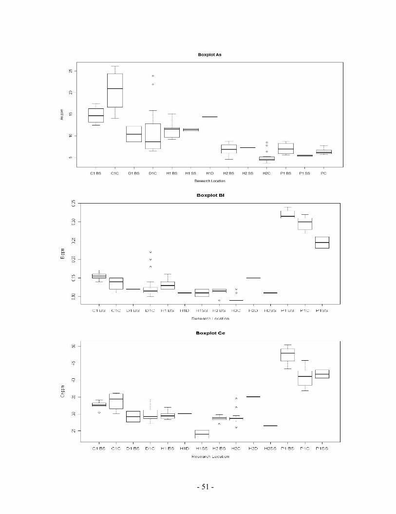
- 51 -

- 52 -

- 53 -

- 54 -

- 55 -

- 56 -

- 57 -

- 58 -

- 59 -

Appendix 3 Regression prediction Cu and Zn

Figure A3.1 Cu: Al plotted for the reference values (vertical profile P1 excluded), the control site C1, BS and SS for sampling sites H1 and H2 and the BS and vertical profile for site P1.

regression prediction Cu 37.999x - 16.365 regression prediction Zn 37.699x + 23.867 p-value regression 2.93 * 10-8 p-value regression 0.042

Average Background concentrations (ppm) 44.51

Average Background concentrations (ppm) 84.08

Standard Error (ppm) 4.97 Standard Error (ppm) 19.16 R2 0.76 R2 0.17

Figure A3.2 Zn: Al plotted for the reference values, the control site C1, BS and SS for sampling sites H1 and H2 and the BS for site P1.

- 60 -

Appendix 4 Enrichment ratio

Mean metal concentrations reference material (ppm) Ag Al As Ba Be Bi Ca Cd Ce Co Cr Cs Cu Fe Ga Ge Hf Hg In K La Li Mg Mn

0.14 1.49 11.54 123.10 0.37 0.16 0.89 0.30 33.06 12.93 42.76 1.45 45.77 3.11 4.52 0.07 0.06 0.07 0.02 0.09 17.42 16.30 0.66 697.34

Mo Na Nb Ni P Pb Rb Re S Sb Sc Se Sn Sr Ta Te Th Ti Tl U V W Y Zn Zr

1.15 0.03 0.92 31.31 1081.72 12.65 9.49 0.00 0.12 0.39 5.89 1.09 1.13 75.13 0.01 0.02 4.19 0.07 0.09 1.21 64.72 0.22 10.27 84.17 2.50 Mean metal concentrations per sampling site

Ag Al As Ba Be Bi Ca Cd Ce Co Cr Cs Cu Fe Ga Ge Hf Hg In K La Li Mg Mn BS H1 0.19 1.73 11.52 198.33 0.42 0.13 1.54 0.48 29.67 12.68 41.50 1.57 97.87 3.01 4.57 0.10 0.04 0.15 0.02 0.11 15.17 13.92 0.63 2440 BS H2 0.16 1.90 6.83 171.67 0.37 0.11 1.28 0.44 28.63 11.98 40.17 1.40 101.25 2.72 5.18 0.09 0.04 0.14 0.02 0.12 14.25 14.30 0.65 4187 BS D1 0.13 1.375 10.4 120 0.345 0.12 0.87 0.34 29.2 12.65 39.5 1.405 47.25 2.84 4.13 0.05 0.04 0.09 0.0195 0.105 16.15 14.95 0.585 1675 BS P1 0.14 0.93 7.08 102.50 0.16 0.32 0.61 0.28 47.40 13.63 17.25 0.53 36.15 3.27 2.68 0.08 0.06 0.02 0.01 0.07 24.80 14.13 0.61 749

SS H1-H2 0.19 1.57 10.03 170.00 0.41 0.11 1.52 0.50 24.83 12.20 32.00 1.46 106.93 2.47 4.30 0.06 0.03 0.16 0.02 0.12 13.60 13.13 0.56 4110 SS P1 0.115 0.72 5.45 80 0.135 0.245 0.725 0.225 41.8 11.5 12.5 0.345 29.05 2.79 2.35 0.08 0.08 0.01 0.013 0.04 21.25 11.75 0.555 608

V-Profile P1 0.15 0.77 6.39 71.11 0.13 0.30 1.11 0.24 40.67 13.11 27.22 0.46 53.44 3.19 2.33 0.05 0.09 0.01 0.02 0.05 21.67 13.16 0.63 709

Mo Na Nb Ni P Pb Rb S Sb Sc Se Sn Sr Te Th Ti Tl U V W Y Zn Zr

BS H1 1.37 0.03 0.91 28.07 1540.00 8.43 9.62 0.16 0.42 5.63 5.73 0.42 137.58 0.04 0.93 0.05 0.10 1.30 68.67 0.23 14.14 155.83 1.02

BS H2 1.42 0.02 0.91 24.45 1588.33 7.53 9.18 0.19 0.31 5.40 4.40 0.45 121.33 0.03 1.27 0.07 0.09 1.11 64.67 0.20 12.03 113.17 1.08

BS D1 0.86 0.03 0.9 27.8 1240 7.15 9.55 0.09 0.31 5 2 0.3 81.2 0.035 2.3 0.0585 0.09 0.86 61 0.27 10.035 85.5 1.1

BS P1 1.01 0.01 0.36 33.03 730.00 21.33 5.30 0.02 0.45 2.03 0.80 <0.2 23.33 0.04 10.08 0.01 0.04 1.20 14.50 0.23 5.76 104.50 3.63

SS H1-H2 1.34 0.03 0.71 26.67 1760.00 7.67 9.97 0.22 0.38 4.33 7.97 3.37 135.33 0.10 0.50 0.04 0.09 0.94 50.00 0.19 11.47 114.33 0.60

SS P1 0.91 0.01 0.295 30.05 675 17.1 3.9 0.02 0.405 1.95 0.6 0.2 26.55 0.04 8.5 0.0095 0.03 0.935 12.5 0.19 4.94 71.5 4.65

V-Profile P1 1.25 0.01 0.27 37.09 646.67 44.56 4.32 0.04 0.47 1.74 0.58 6.06 42.86 0.04 9.50 0.01 0.04 1.15 12.78 0.53 4.90 83.00 5.32

- 61 -

Resulting Simple Enrichment ratios. Red indicates high enrichment, orange middle, or only for Cariboo ares, green indicates no enrichment.

Enrichment ratios Ag Al As Ba Be Bi Ca Cd Ce Co Cr Cs Cu Fe Ga Ge Hf Hg In K La Li Mg

BS H1 1.35

1.16

1.00 1.61

1.13

0.85

1.72 1.59

0.90 0.98

0.97

1.08

2.14

0.97

1.01 1.37

0.65

1.99

1.14 1.25 0.87 0.85 0.95

BS H2 1.13

1.27

0.59 1.39

0.98

0.71

1.43 1.44

0.87 0.93

0.94

0.96

2.21

0.87

1.14 1.23

0.65

1.85

1.03 1.29 0.82 0.88 0.98

BS P1 1.00

0.62

0.61 0.83

0.42

2.03

0.68 0.91

1.43 1.05

0.40

0.36

0.79

1.05

0.59 1.05

1.02

0.20

0.68 0.76 1.42 0.87 0.91

BS D1 0.93

0.92

0.90 0.97

0.92

0.76

0.97 1.12

0.88 0.98

0.92

0.97

1.03

0.91

0.91 0.70

0.65

1.22

0.90 1.18 0.93 0.92 0.88

SS 1.36

1.05

0.87 1.38

1.09

0.70

1.70 1.65

0.75 0.94

0.75

1.01

2.34

0.80

0.95 0.88

0.49

2.17

0.88 1.38 0.78 0.81 0.85

SS (P1) 0.82

0.48

0.47 0.65

0.36

1.55

0.81 0.74

1.26 0.89

0.29

0.24

0.63

0.90

0.52 1.12

1.30

0.14

0.60 0.45 1.22 0.72 0.84

Vertical Profile P1 1.05

0.52

0.55 0.58

0.35

1.88

1.24 0.78

1.23 1.01

0.64

0.32

1.17

1.03

0.51 0.70

1.39

0.15

0.78 0.56 1.24 0.81 0.95

Enrichment ratios Mn Mo Na Nb Ni P Pb Rb S Sb Sc Se Sn Sr Te Th Ti Tl U V W Y Zn Zr

BS H1 3.50 1.19 1.05 0.99 0.90 1.42 0.67 1.01 1.35 1.07 0.96 5.28 0.37 1.83 1.78 0.22 0.83 1.08 1.08 1.06 1.04 1.38 1.85 0.41 BS H2 6.00 1.24 0.87 0.98 0.78 1.47 0.60 0.97 1.53 0.79 0.92 4.05 0.40 1.62 1.14 0.30 1.01 0.97 0.92 1.00 0.89 1.17 1.34 0.43 BS P1 1.08 0.88 0.37 0.39 1.05 0.67 1.69 0.56 0.12 1.15 0.34 0.74 0.31 1.71 2.40 0.17 0.47 0.99 0.22 1.03 0.56 1.24 1.45 BS D1 2.40 0.75 1.12 0.98 0.89 1.15 0.57 1.01 0.74 0.79 0.85 1.84 0.27 1.08 1.49 0.55 0.89 0.99 0.71 0.94 1.21 0.98 1.02 0.44

SS 5.89 1.17 1.24 0.77 0.85 1.63 0.61 1.05 1.82 0.97 0.74 7.33 2.98 1.80 4.26 0.12 0.55 0.96 0.78 0.77 0.84 1.12 1.36 0.24 SS (P1) 0.87 0.79 0.37 0.32 0.96 0.62 1.35 0.41 0.17 1.04 0.33 0.55 0.18 0.35 1.71 2.03 0.14 0.33 0.77 0.19 0.85 0.48 0.85 1.86

Vertical Profile P1 1.02 1.09 0.37 0.29 1.18 0.60 3.52 0.46 0.32 1.20 0.30 0.53 5.35 0.57 1.71 2.27 0.14 0.43 0.95 0.20 2.36 0.48 0.99 2.13

- 62 -

Enrichment calculated by dividing the actual metal concentration by the regression prediction. Enrichment

ratios Al Ba Prediction ER Bi Prediction ER Ca Prediction Cd Prediction ER Ce Prediction ER Cu Prediction ER

BS H1 1.73 198.33 137.23 1.45 0.13 0.13 1.04 1.54 0.97 0.48 0.33 1.47 29.67 31.08 0.95 97.87 47.62 2.06 BS H2 1.90 171.67 146.82 1.17 0.11 0.11 1.04 1.28 0.95 0.44 0.35 1.26 28.63 29.74 0.96 101.25 48.87 2.07 BS P1 0.93 102.50 90.34 1.13 0.32 0.23 1.41 0.61 1.06 0.28 0.24 1.14 47.40 37.63 1.26 36.15 41.49 0.87 BS D1 1.38 120.00 116.50 1.03 0.12 0.17 0.70 0.87 1.01 0.34 0.29 1.17 29.20 33.98 0.86 47.25 44.91 1.05

SS 1.57 170.00 127.83 1.33 0.11 0.15 0.75 1.52 0.99 0.50 0.31 1.60 24.83 32.39 0.77 106.93 46.39 2.31 SS (P1) 0.72 80.00 78.42 1.02 0.25 0.25 0.98 0.73 1.09 0.23 0.22 1.02 41.80 39.30 1.06 29.05 39.93 0.73

Vertical Profile P1 1.37 71.11 116.19 0.61 0.30 0.17 1.72 1.11 1.01 0.24 0.29 0.82 40.67 34.02 1.20 53.44 44.87 1.19

Enrichment

ratios Hg Prediction ER Mn Prediction ER P Prediction ER Pb Prediction ER S Prediction ER Se Prediction ER

BS H1 0.15 0.10 1.54 2440.00 688.18 3.55 1540.00 1208.85 1.27 8.43 9.20 0.92 0.16 0.15 1.07 5.28 1.25 4.23 BS H2 0.14 0.11 1.25 4186.67 681.95 6.14 1588.33 1295.15 1.23 7.53 9.46 0.80 0.19 0.17 1.06 4.05 1.36 2.98 BS P1 0.02 0.02 0.62 749.75 718.60 1.04 730.00 786.92 0.93 21.33 7.95 2.68 0.02 0.05 0.32 0.74 0.71 1.04 BS D1 0.09 0.06 1.41 1675.00 701.63 2.39 1240.00 1022.29 1.21 7.15 8.65 0.83 0.09 0.11 0.85 1.84 1.01 1.82

SS 0.16 0.08 1.98 4110.00 694.27 5.92 1760.00 1124.29 1.57 7.67 8.95 0.86 0.22 0.13 1.67 7.33 1.14 6.43 SS (P1) 0.01 0.01 1.62 608.00 726.33 0.84 675.00 679.70 0.99 17.10 7.63 2.24 0.02 0.02 0.97 0.55 0.57 0.97 Vertical

Profile P1 0.01 0.06 0.18 709.00 701.83 1.01 646.67 1019.53 0.63 44.56 8.64 5.16 0.04 0.11 0.37 0.53 1.01 0.53

Enrichment ratios Sn Prediction ER Sr Prediction ER Te Prediction ER Th Prediction ER Zr Prediction ER Zn Prediction ER

BS H1 0.42 0.41 1.01 137.58 84.28 1.63 0.04 0.02 1.99 0.93 3.00 0.31 1.02 2.05 0.50 155.83 87.37 1.78 BS H2 0.45 0.42 1.08 121.33 90.49 1.34 0.03 0.02 1.39 1.27 2.67 0.48 1.08 2.10 0.52 113.17 89.54 1.26 BS P1 0.00 0.40 0.00 23.33 53.91 0.43 0.04 0.03 1.35 10.08 4.66 2.16 3.63 1.84 1.97 104.50 76.76 1.36

- 63 -

BS D1 0.30 0.41 0.73 81.20 70.85 1.15 0.04 0.02 1.41 2.30 3.74 0.62 1.10 1.96 0.56 85.50 82.68 1.03 SS 3.37 0.41 8.18 135.33 78.19 1.73 0.10 0.02 4.42 0.50 3.34 0.15 0.60 2.01 0.30 114.33 85.24 1.34

SS (P1) 0.20 0.40 0.50 26.55 46.19 0.57 0.04 0.03 1.26 8.50 5.08 1.67 4.65 1.78 2.61 71.50 74.06 0.97 Vertical

Profile P1 6.06 0.41 14.81 42.86 70.65 0.61 0.04 0.02 1.61 9.50 3.75 2.54 5.32 1.95 2.72 83.00 82.61 1.00 Appendix 5 Regression analyses

Enrichment Factor Al - Ba

y = 58.132x + 36.567

0

50

100

150

200

250

300

0 0.5 1 1.5 2 2.5Al (ppm)

Ba (p

pm)

Reference ValuesBS C1BS H1BS H2BS P1SSSS P1Vertical Profile P1Lineair (Reference Values)

Enrichment Factor Al - Bi

y = -0.1219x + 0.339

0

0.05

0.1

0.15

0.2

0.25

0.3

0.35

0.4

0 0.5 1 1.5 2 2.5Al (ppm)

Bi (p

pm)

Reference ValuesBS C1BS H1BS H2BS P1SSSS P1Verical Profile P1Lineair (Reference Values)

- 64 -

Enrichment Factor Al - Ca

y = -0.1884x + 1.1742

0

0.2

0.4

0.6

0.8

1

1.2

1.4

1.6

1.8

0 0.5 1 1.5 2 2.5Al (ppm)

Ca (p

pm)

Reference ValuesBS C1BS H1BS H2BS P1SSSS P1Verical Profile P1Lineair (Reference Values)

Enrichment Factor Al - Cd

y = 0.1074x + 0.1439

0

0.1

0.2

0.3

0.4

0.5

0.6

0 0.5 1 1.5 2 2.5Al (ppm)

Cd (p

pm)

Reference ValuesBS H1BS H2BS P1BS D1BS C1SSSS P1Vertical Profile P1Lineair (Reference Values)

Enrichment Factor Al - Ce

y = -8.1179x + 45.14

0

10

20

30

40

50

60

0 0.5 1 1.5 2 2.5Al (ppm)

Ce

(ppm

)

Reference ValuesBS C1BS H1BS H2BS P1SSSS P1Verical Profile P1Lineair (Reference Values)

Enrichment Factor Al - Cu

y = 7.6007x + 34.458

0

20

40

60

80

100

120

0 0.5 1 1.5 2 2.5Al (ppm)

Cu (p

pm)

Reference ValuesBS H1BS H2BS P1BS D1BS C1SSSS P1Vertical Profile P1Lineair (Reference Values)

- 65 -

Enrichment Factor Al - Hg

y = 0.0879x - 0.0571

0

0.02

0.04

0.06

0.08

0.1

0.12

0.14

0.16

0.18

0.2

0 0.5 1 1.5 2 2.5Al (ppm)

Hg (p

pm)

Reference ValuesBS H1BS H2BS P1BS D1BS C1SSSS P1Vertical Profile P1Lineair (Reference Values)

Enrichment Factor Al - Mn

y = -37.717x + 753.49

0

1000

2000

3000

4000

5000

6000

7000

0 0.5 1 1.5 2 2.5Al (ppm)

Mn

(ppm

)

Reference ValuesBS H1BS H2BS P1BS D1BS C1SSSS P1Vertical Profile P1Lineair (Reference Values)

Enrichment Factor Al - P

y = 523.05x + 303.1

0200400600800

100012001400160018002000

0 0.5 1 1.5 2 2.5Al (ppm)

P (

pp

m)

Reference ValuesBS C1BS H1BS H2BS P1SSSS P1Verical Profile P1Lineair (Reference Values)

Enrichment Factor Al - S

y = 0.1306x - 0.0734

0

0.1

0.2

0.3

0.4

0.5

0.6

0 0.5 1 1.5 2 2.5Al (ppm)

S (p

pm)

Reference ValuesBS H1BS H2BS P1BS D1BS C1SSSS P1Vertical Profile P1Lineair (Reference Values)

- 66 -

Enrichment Factor Al - Se

y = 0.6696x + 0.0895

0

1

2

3

4

5

6

7

8

9

10

0 0.5 1 1.5 2 2.5Al (ppm)

Se (p

pm)

Reference ValuesBS H1BS H2BS P1BS D1BS C1SSSS P1Vertical Profile P1Lineair (Reference Values)

Enrichment Factor Al - Sr

y = 37.646x + 19.088

0

20

40

60

80

100

120

140

160

0 0.5 1 1.5 2 2.5Al (ppm)

Sr (p

pm)

Reference ValuesBS C1BS H1BS H2BS P1SSSS P1Verical Profile P1Lineair (Reference Values)

Enrichment Factor Al - Sn

y = 0.014x + 0.3896

0

1

2

3

4

5

6

7

8

9

0 0.5 1 1.5 2 2.5Al (ppm)

Sn (p

pm)

Reference ValuesBS C1BS H1BS H2BS P1SSSS P1Verical Profile P1Lineair (Reference Values)

Enrichment Factor Al - Te

y = -0.0108x + 0.0396

0

0.02

0.04

0.06

0.08

0.1

0.12

0.14

0.16

0 0.5 1 1.5 2 2.5Al (ppm)

Te (p

pm)

Reference ValuesBS C1BS H1BS H2BS P1SSSS P1Verical Profile P1Lineair (Reference Values)

- 67 -

Enrichment Factor Al - Th

y = -2.0525x + 6.5583

0

2

4

6

8

10

12

0 0.5 1 1.5 2 2.5Al (ppm)

Th (p

pm)

Reference ValuesBS C1BS H1BS H2BS P1SSSS P1Verical Profile P1Lineair (Reference Values)

Enrichment Factor Al - Zr

y = 0.2686x + 1.587

0

1

2

3

4

5

6

7

8

0 0.5 1 1.5 2 2.5Al (ppm)

Zr (p

pm)

Reference ValuesBS C1BS H1BS H2BS P1SSSS P1Verical Profile P1Lineair (Reference Values)

Enrichment Factor Al - Zn

y = 13.155x + 64.59

0

50

100

150

200

250

0 0.5 1 1.5 2 2.5Al (ppm)

Zn (p

pm)

Reference ValuesBS H1BS H2BS P1BS D1BS C1SSSS P1SS Vertical ProfileLineair (Reference Values)

68

Appendix 6 coring H2 Coring H2 with two active mining periods highlighted. Red color is the first period 1997-2001 and the green color denotes the second period, 2005-present. The horizontal axis denotes depth below the surface (cm). The vertical axis denotes amount of metal content (ppm).

As

02468

101214161820

0 2 4 6 8 10

As

Cd

02468

101214161820

0 0.1 0.2 0.3 0.4

Cd

Cu

02468

101214161820

0 20 40 60 80 100

Cu

Fe

02468

101214161820

0 0.5 1 1.5 2 2.5 3 3.5

Fe

Hg

02468

101214161820

0 0.02 0.04 0.06 0.08 0.1 0.12 0.14

Hg

Mn

02468

101214161820

0 200 400 600 800 1000 1200

Mn

Pb

02468

101214161820

0 2 4 6 8 10 12 14

Pb

Se

02468

101214161820

0 0.5 1 1.5 2 2.5 3

Se

Zn

02468

101214161820

0 20 40 60 80 100

Zn

69

Elevated heavy metal concentrations for the first active mining period and the reference values plotted against aluminum for As, Cd, Cu, Mn and Se.

Al:As

0

5

10

15

20

25

30

0 0,5 1 1,5 2 2,5

Al (ppm)

As (p

pm)

Reference ValuesFirst Active Mining Period:

Al:Cd

0

0,1

0,2

0,3

0,4

0,5

0,6

0 0,5 1 1,5 2 2,5

Al (ppm)

Cd (p

pm)

Reference ValuesFirst Active Mining Period:

Al:Cu

0

10

20

30

40

50

60

70

80

0 0,5 1 1,5 2 2,5

Al (ppm)

Cu (p

pm)

Reference ValuesFirst Active Mining Period:

Al:Mn

0

200

400

600

800

1000

1200

1400

1600

1800

0 0,5 1 1,5 2 2,5

Al (ppm)

Mn

(ppm

)

Reference ValuesFirst Active Mining Period:

Al:Se

y = 0,6696x + 0,0895

0

0,2

0,4

0,6

0,8

1

1,2

1,4

1,6

1,8

2

0 0,5 1 1,5 2 2,5

Al (ppm)

Se (p

pm)

Reference ValuesFirst Active Mining Period: Linear (Reference Values)

70

Appendix 7 Naturally occuring heavy metal concentrations in igneous rocks (ppm) and sedimentray Rocks (Adriano (1995), van der Perk (2006)).

Metal Average concentration Range As 1.5-3 0.06-113 Cd 0.082 0.001-0.60 Pb 15 2-30 Hg - 5-250 Cu - 10-100 Mn - 390-1620 Zn 65 5-1070 Ni 75 2-3600 Se 0.05 -

Igneous Rocks Sedimentary Rocks Ultramafic

(mg/kg) Mafic (mg/kg)

Granitic (mg/kg)

Limestone (mg/kg)

Sandstone (mg/kg)

Shales/Clays (mg/kg)

Fresh Water (µg/l)

As 1 1.5 1.5 2.6 4.1 13 0.2-230 Cd 0.12 0.13 0.09 0.028 0.05 0.22 0.01-3 Cr 2980 200 4 11 35 39 0.1-6 Cu 42 90 13 5.5 30 39 2-30 Hg 0.0004 0.01 0.08 0.16 0.29 0.18 0.00001-2.8 Ni 2000 150 0.5 7 9 68 0.02-27 Pb 14 3 24 5.7 10 23 0.06-120 Sn 0.5 1.5 3.5 0.5 0.5 6 0.0004-0.09 Zn 58 100 52 20 30 120 0.2-100

Appendix 8 Stored fine sediment per sampling site, for every round of bed sediments taken.

Sampling Site

round 1 (g/m2)

round 2 (g/m2)

round 3 (g/m2)

round 4 (g/m2)

round 5 (g/m2)

round 6 (g/m2)

average (g/m2)

H1 149,40 68,47 70,71 168,93 137,79 102,37 116,28 H2 333,20 520,31 124,85 333,13 841,07 181,41 388,99 D1 282,09 1264,95 773,53 C1 252,24 279,44 159,73 378,50 173,85 326,55 261,72 P1 270,35 303,25 141,35 210,92 231,47