J Glob Optim (2013) 56:1247–1293DOI 10.1007/s10898-012-9951-y

Derivative-free optimization: a review of algorithmsand comparison of software implementations

Luis Miguel Rios · Nikolaos V. Sahinidis

Received: 20 December 2011 / Accepted: 23 June 2012 / Published online: 12 July 2012© Springer Science+Business Media, LLC. 2012

Abstract This paper addresses the solution of bound-constrained optimization problemsusing algorithms that require only the availability of objective function values but no deriv-ative information. We refer to these algorithms as derivative-free algorithms. Fueled by agrowing number of applications in science and engineering, the development of derivative-free optimization algorithms has long been studied, and it has found renewed interest inrecent time. Along with many derivative-free algorithms, many software implementationshave also appeared. The paper presents a review of derivative-free algorithms, followed bya systematic comparison of 22 related implementations using a test set of 502 problems.The test bed includes convex and nonconvex problems, smooth as well as nonsmooth prob-lems. The algorithms were tested under the same conditions and ranked under several crite-ria, including their ability to find near-global solutions for nonconvex problems, improve agiven starting point, and refine a near-optimal solution. A total of 112,448 problem instanceswere solved. We find that the ability of all these solvers to obtain good solutions dimin-ishes with increasing problem size. For the problems used in this study, TOMLAB/MULTI-MIN, TOMLAB/GLCCLUSTER, MCS and TOMLAB/LGO are better, on average, than otherderivative-free solvers in terms of solution quality within 2,500 function evaluations. Theseglobal solvers outperform local solvers even for convex problems. Finally,TOMLAB/OQNLP,NEWUOA, and TOMLAB/MULTIMIN show superior performance in terms of refining a near-optimal solution.

Keywords Derivative-free algorithms · Direct search methods · Surrogate models

Electronic supplementary material The online version of this article (doi:10.1007/s10898-012-9951-y)contains supplementary material, which is available to authorized users.

L. M. Rios · N. V. Sahinidis (B)Department of Chemical Engineering,Carnegie Mellon University, Pittsburgh, PA 15213, USAe-mail: sahinidis@cmu.edu

L. M. Riose-mail: lmrios@gmail.com

123

1248 J Glob Optim (2013) 56:1247–1293

1 Introduction

The problem addressed in this paper is the optimization of a deterministic function f :R

n → R over a domain of interest that possibly includes lower and upper bounds on theproblem variables. We assume that the derivatives of f are neither symbolically nor numeri-cally available, and that bounds, such as Lipschitz constants, for the derivatives of f are alsounavailable.

The problem is of interest when derivative information is unavailable, unreliable, orimpractical to obtain, for instance when f is expensive to evaluate or somewhat noisy,which renders most methods based on finite differences of little or no use [79,140]. We referto this problem as derivative-free optimization. We further refer to any algorithm applied tothis problem as a derivative-free algorithm, even if the algorithm involves the computationof derivatives for functions other than f .

Derivative-free optimization is an area of long history and current rapid growth, fueled bya growing number of applications that range from science problems [4,42,52,143] to medicalproblems [90,103] to engineering design and facility location problems [2,10,15,48,49,54,57,91,92,98].

The development of derivative-free algorithms dates back to the works of Spendley et al.[132] and Nelder and Mead [99] with their simplex-based algorithms. Recent works on thesubject have led to significant progress by providing convergence proofs [5,9,31,34,76,80,85,88,134], incorporating the use of surrogate models [22,24,127,131], and offering thefirst textbook that is exclusively devoted to this topic [35]. Concurrent with the develop-ment of algorithms, software implementations for this class of optimization problems haveresulted in a wealth of software packages, including BOBYQA [115], CMA-ES [55], fourCOLINY solvers [124], DFO [125], glcCluster [60, pp. 109–111], HOPSPACK [108],IMFIL [74], LGO [105], MCS [101], multiMin [60, pp. 148-151], NEWUOA [114],NOMAD [6], OQNLP [62], PSWARM [137,138], SID-PSM [40,41], and SNOBFIT [66].

Mongeau et al. [96] performed a comparison of derivative-free solvers in 1998 by con-sidering six solvers over a set of eleven test problems. Since the time of that comparison, thenumber of available derivative-free optimization solvers has more than quadrupled. Othercomparisons, such as [11,33,38,48,53,65,67,97,138], are restricted to a few solvers relatedto the algorithms proposed in these papers. In addition, these comparisons consider smallsets of test problems. There is currently no systematic comparison of the existing implemen-tations of derivative-free optimization algorithms on a large collection of test problems. Theprimary purpose of the present paper is to provide such a comparison, aiming at addressingthe following questions:

– What is the quality of solutions obtained by current solvers for a given limit on the num-ber of allowable function evaluations? Does quality drop significantly as problem sizeincreases?

– Which solver is more likely to obtain global or near-global solutions for nonconvexproblems?

– Is there a subset of existing solvers that would suffice to solve a large fraction of problemswhen all solvers are independently applied to all problems of interest? Conversely, arethere problems that can be solved by only one or a few solvers?

– Given a starting near-optimal solution, which solver reaches the solution fastest?

Before addressing these questions computationally, the paper begins by presenting areview of the underlying theory and motivational ideas of the algorithms. We classify algo-rithms developed for this problem as direct and model-based. Direct algorithms determine

123

J Glob Optim (2013) 56:1247–1293 1249

search directions by computing values of the function f directly, whereas model-based algo-rithms construct and utilize a surrogate model of f to guide the search process. We furtherclassify algorithms as local or global, with the latter having the ability to refine the searchdomain arbitrarily. Finally, we classify algorithms as stochastic or deterministic, dependingupon whether they require random search steps or not.

Readers familiar with the subject matter of this paper may have noticed that there existsliterature that reserves the term derivative-free algorithms only for what we refer to as model-based algorithms in the current paper. In addition, what we refer to as derivative-free opti-mization is often also referred to as optimization over black boxes. The literature on theseterms is often inconsistent and confusing (cf. [79] and discussion therein).

Local search algorithms are reviewed in Sect. 2. The presentation includes direct andmodel-based strategies. Global search algorithms are discussed in Sect. 3, including deter-ministic as well as stochastic approaches. Section 4 provides a brief historical overview andoverall assessment of the algorithmic state-of-the-art in this area. Leading software imple-mentations of derivative-free algorithms are discussed in Sect. 5. The discussion includessoftware characteristics, requirements, and types of problems handled. Extensive computa-tional experience with these codes is presented in Sects. 6 and 7. A total of 502 test problemswere used, including 78 smooth convex, 161 nonsmooth convex, 245 smooth nonconvex,and 18 nonsmooth nonconvex problems. These problems were used to test 22 solvers usingthe same starting points and bounding boxes. During the course of the computational workfor this paper, we made test problems and results available to the software developers andasked them to provide us with a set of options of their choice. Many of them responded andeven decided to change the default settings in their software thereafter. In an effort to encour-age developers to revise and improve their software, we shared our computational resultswith them over several rounds. Between each round, several developers provided improvedversions of their implementations. At the end of this process, we tested their software againstan additional collection of problems that had not been seen by developers in order to confirmthat the process had not led to overtraining of the software on our test problem collection.Conclusions from this entire study are drawn in Sect. 8.

2 Local search methods

2.1 Direct local search methods

Hooke and Jeeves [64] describe direct search as the sequential examination of trial solu-tions generated by a certain strategy. Classical direct search methods did not come withproofs of termination or convergence to stationary points. However, recent papers start-ing with [134,135] have proved convergence to stationary points, among other properties.These old methods remain popular due to their simplicity, flexibility, and reliability. We nextdescribe specific direct search methods that are local in nature.

2.1.1 Nelder–Mead simplex algorithm

The Nelder–Mead algorithm introduced in [99] starts with a set of points that form a simplex.In each iteration, the objective function values at the corner points of the simplex determinethe worst corner point. The algorithm attempts to replace the worst point by introducing anew vertex in a way that results in a new simplex. Candidate replacement points are obtainedby transforming the worst vertex through a number of operations about the centroid of the

123

1250 J Glob Optim (2013) 56:1247–1293

current simplex: reflection, expansion, inside and outside contractions. McKinnon [94] hasestablished analytically that convergence of the Nelder–Mead algorithm can occur to a pointwhere the gradient of the objective function is nonzero, even when the function is convex andtwice continuously differentiable. To prevent stagnation, Kelley [75] proposed to enforce asufficient decrease condition determined by an approximation of the gradient. If stagnationis observed, the algorithm restarts from a different simplex. Tseng [136] proposed a glob-ally convergent simplex-based search method that considers an expanded set of candidatereplacement points. Other modifications of the Nelder–Mead algorithm are presented in [35].

2.1.2 Generalized pattern search (GPS) and generating set search (GSS) methods

Torczon [135] introduced generalized pattern search methods (GPS) for unconstrained opti-mization. GPS generalizes direct search methods including the Hooke and Jeeves [64] algo-rithm. At the beginning of a new iteration, GPS searches by exploratory moves. The currentiterate defines a set of points that form a pattern, determined by a step and a generatingmatrix that spans R

n .Further generalizing GPS, Kolda et al. [79] coined the term GSS in order to describe, unify,

and analyze direct search methods, including algorithms that apply to constrained problems.Each iteration k of GSS methods consists of two basic steps. The search step is performedfirst over a finite set of search directions Hk generated by some, possibly heuristic, strategythat aims to improve the current iterate but may not guarantee convergence. If the search stepfails to produce a better point, GSS methods continue with the poll step, which is associatedwith a generating set Gk that spans positively R

n . Generating sets are usually positive bases,with a cardinality between n + 1 to 2n. Assuming f is smooth, a generating set contains atleast one descent direction of f at a non-stationary point in the domain of definition of f .

Given G = {d(1), . . . , d(p)} with p ≥ n + 1 and d(i) ∈ Rn , the function f is evaluated

at a set of trial points Pk = {xk + �kd : d ∈ Gk}, where �k is the step length. An iterationis successful if there exists y ∈ Pk such that f (y) < f (xk) − ρ(�k), where ρ is a forcingfunction. The opportunistic poll strategy proceeds to the next iteration upon finding a point y,while the complete poll strategy evaluates all points in Pk and assigns y = arg minx∈Pk f (x).Successful iterations update the iterate xk+1 to y and possibly increase the step length �k+1

to φk�k , with φk ≥ 1. Unsuccessful iterations maintain the same iterate, i.e., xk+1 = xk , andreduce the step length �k+1 to θk�k , with 0 < θk < 1. The forcing function ρ is included inorder to impose a sufficient decrease condition and is required to be a continuous decreasingfunction with limt→0 ρ(t)/t = 0. Alternatively, the set Pk can be generated using integerlattices [135]. In the latter case, the iteration is successful if a point y satisfies simple decrease,i.e., f (y) < f (xk).

Lewis and Torczon [83] extended pattern search methods to problems with bound con-straints by including axis directions in the set of poll directions. Lewis and Torczon [84]further extended pattern search methods to linearly constrained problems by forcing the gen-erating set to span a tangent cone T�(xk, ε), which restricts the tangent vectors to satisfy allconstraints within an ε-neighborhood from xk .

Under mild conditions, [135] showed convergence of GSS methods to stationary points,which, could be local minima, local maxima, or even saddle points.

Mesh adaptive direct search (MADS) methods The MADS methods (Audet and Dennis [11])modified the poll step of GPS algorithms to consider a variable set of poll directions whoseunion across all iterations is asymptotically dense in R

n . MADS generates the poll pointsusing two parameters: a poll size parameter, which restricts the region from which points can

123

J Glob Optim (2013) 56:1247–1293 1251

be selected, and a mesh size parameter, which defines a grid inside the region limited by thepoll size parameter. MADS incorporates dynamic ordering, giving precedence to previouslysuccessful poll directions. Audet and Dennis [11] first proposed random generation of polldirections for each iteration, and Audet et al. [8] proposed a deterministic way for generatingorthogonal directions.

Abramson and Audet [5] showed convergence of the MADS method to second-orderstationary points under the assumption that f is continuously differentiable with Lipschitzderivatives near the limit point. Under additional assumptions ( f twice strictly differentiablenear the limit point), MADS was shown to converge to a local minimizer with probability 1.A number of problems for which GPS stagnates and MADS converges to an optimal solutionare presented in [11]. Some examples were presented in [5] that show how GPS methodsstall at saddle points, while MADS escapes and converges to a local minimum.

MADS handles general constraints by the extreme barrier approach [11], which rejectsinfeasible trial points from consideration, or by the progressive barrier approach [12], whichallows infeasible trial points within a decreasing infeasibility threshold.

Pattern search methods using simplex gradients Custódio and Vicente [40] proposed toenhance the poll step by giving preference to directions that are closest to the negative ofthe simplex gradient. Simplex gradients are an approximation to the real gradient and arecalculated out of a simplex defined by previously evaluated points.

2.2 Local model-based search algorithms

The availability of a high-fidelity surrogate model permits one to exploit its underlying prop-erties to guide the search in a intelligent way. Properties such as the gradient and higher orderderivative information, as well as the probability distribution function of the surrogate modelare used. Since a high-fidelity surrogate model is typically unavailable for a given problem,these methods start by sampling the search space and building an initial surrogate model.The methods then proceed iteratively to optimize the surrogate model, evaluate the solutionpoint, and update the surrogate model.

2.2.1 Trust-region methods

Trust-region methods use a surrogate model that is usually smooth, easy to evaluate, andpresumed to be accurate in a neighborhood (trust region) about the current iterate. Powell[109] proposed to use a linear model of the objective within a trust-region method. The algo-rithm considered a monotonically decreasing radius parameter and included iterations thatmaintained geometric conditions of the interpolation points. Linear models are practical sincethey only require O(n) interpolation points, albeit at the cost of not capturing the curvatureof the underlying function. Powell [112] and Conn et al. [31,32] proposed to use a quadraticmodel of the form:

qk(xk + s) = f (xk) + 〈gk, s〉 + 1

2〈s, Hks〉

where, at iteration k, xk is the current iterate, gk ∈ Rn , and Hk is a symmetric matrix of

dimension n. Rather than using derivative information, gk and Hk are estimated by requiringqk to interpolate a set Y of sample points: qk(x (i)) = f (x (i)) for i = 1, . . . , p. Unlessconditions are imposed on the elements of gk and Hk , at least (n + 1)(n + 2)/2 points areneeded to determine gk and Hk uniquely. Let x∗ denote a minimizer of qk within the trust

123

1252 J Glob Optim (2013) 56:1247–1293

region and define the ratio ρk = ( f (xk) − f (x∗)) / (qk(xk) − qk(x∗)). If ρk is greater than auser-defined threshold, x∗ replaces a point in Y and the trust region is increased. Otherwise,if the geometry of the set Y is adequate, the trust-region radius is reduced, while, if the geom-etry is not adequate, a point in the set is replaced by another that improves the poisedness ofthe set. The algorithm terminates when the trust-region radius drops below a given tolerance.

Powell [113] proposed an algorithm that uses a quadratic model relying on fewer than(n +1)(n +2)/2 interpolation points. The remaining degrees of freedom in the interpolationare determined by minimizing the change to the Hessian of the surrogate model between twoconsecutive iterations.

2.2.2 Implicit filtering

In addition to, or instead of developing a surrogate of f , one may develop a surrogate of thegradient of f and use it to expedite the search. Implicit filtering [50,142] uses an approx-imation of the gradient to guide the search, resembling the steepest descent method whenthe gradient is known. The approximation of the gradient at an iterate is based on forwardor centered differences, and the difference increment varies as the optimization progresses.Forward differences require n function evaluations, whereas centered difference gradientsrequire 2n function evaluations over the set {x ± sei : i = 1, . . . , n}, where x is the currentiterate, s is the scale of the stencil, and ei are coordinate unit vectors. As these points aredistributed around the iterate, they produce approximations less sensitive to noise than for-ward differences [50]. A line search is then performed along the direction of the approximategradient. The candidate point is required to satisfy a minimum decrease condition of the formf (x − δ∇s f (x)) − f (x) < −αδ‖∇s f (x)‖2, where δ is the step and α is a parameter. Thealgorithm continues until no point satisfies the minimum decrease condition, at which pointthe scale s is decreased. The implicit filtering algorithm terminates when the approximategradient is less than a certain tolerance proportional to s.

3 Global search algorithms

3.1 Deterministic global search algorithms

3.1.1 Lipschitzian-based partitioning techniques

Lipschitzian-based methods construct and optimize a function that underestimates the orig-inal one. By constructing this underestimator in a piecewise fashion, these methods providepossibilities for global, as opposed to only local, optimization of the original problem. LetL > 0 denote a Lipschitz constant of f . Then | f (a) − f (b)| ≤ L ‖ a − b ‖ for all a, bin the domain of f . Assuming L is known, Shubert [129] proposed an algorithm for bound-constrained problems. This algorithm evaluates the extreme points of the search space andconstructs linear underestimators by means of the Lipschitz constant. The algorithm thenproceeds to evaluate the minimum point of the underestimator and construct a piecewiseunderestimator by partitioning the search space.

A straightforward implementation of Shubert’s algorithm for derivative-free optimiza-tion problems has two major drawbacks: the Lipschitz constant is unknown and the num-ber of function evaluations increases exponentially, as the number of extreme points of ann-dimensional hypercube is 2n . The DIRECT algorithm and branch-and-bound search aretwo possible approaches to address these challenges.

123

J Glob Optim (2013) 56:1247–1293 1253

The DIRECT algorithm Jones et al. [72] proposed the DIRECT algorithm (DIvide a hyper-RECTangle), with two main ideas to extend Shubert’s algorithm to derivative-free optimiza-tion problems. First, function values are computed only at the center of an interval, insteadof all extreme points. By subdividing intervals into thirds, one of the resulting partition ele-ments inherits the center of the initial interval, where the objective function value is alreadyknown. The second main idea of the DIRECT algorithm is to select from among currenthyperrectangles one that (a) has the lowest objective function value for intervals of similarsize and (b) is associate with a large potential rate of decrease of the objective function value.The amount of potential decrease in the current objective function value represents a setableparameter in this algorithm and can be used to balance local and global search; larger valuesensure that the algorithm is not local in its orientation.

In the absence of a Lipschitz constant, the DIRECT algorithm terminates once the numberof iterations reaches a predetermined limit. Under mild conditions, Finkel and Kelley [47]proved that the sequence of best points generated by the algorithm converges to a KKTpoint. Convergence was also established for general constrained problems, using a barrierapproach.

Branch-and-bound (BB) search BB sequentially partitions the search space, and determineslower and upper bounds for the optimum. Partition elements that are inferior are eliminatedin the course of the search. Let Ω = [xl , xu] be the region of interest and let x∗

Ω ∈ Ω be aglobal minimizer of f in Ω . The availability of a Lipschitz constant L along with a set ofsample points = {x (i), i = 1, . . . , p} ⊂ Ω provides lower and upper bounds:

maxi=1,...,p

{ f (x (i)) − Lδi } = fΩ

≤ f (x∗Ω) ≤ f Ω = min

i=1,...,pf (x (i)),

where δi is a function of the distance of x (i) from the vertices of [xl , xu]. The Lipschitzconstant L is unknown but a lower bound L can be estimated from the sampled objectivefunction values:

L = maxi, j

| f (x (i)) − f (x ( j))|‖x (i) − x ( j)‖ ≤ L , i, j = 1, . . . , p, i = j.

Due to the difficulty of obtaining deterministic upper bounds for L , statistical bounds rely-ing on extreme order statistics were proposed in [106]. This approach assumes samples aregenerated randomly from � and their corresponding objective function values are randomvariables. Subset-specific estimates of L can be significantly smaller than the global L , thusproviding sharper lower bounds for the objective function as BB iterations proceed.

3.1.2 Multilevel coordinate search (MCS)

Like the DIRECT algorithm, MCS [65] partitions the search space into boxes with an eval-uated base point. Unlike the DIRECT algorithm, MCS allows base points anywhere in thecorresponding boxes. Boxes are divided with respect to a single coordinate. The global-localsearch that is conducted is balanced by a multilevel approach, according to which each boxis assigned a level s that is an increasing function of the number of times the box has beenprocessed. Boxes with level s = smax are considered too small to be further split.

At each iteration, MCS selects boxes with the lowest objective value for each level valueand marks them as candidates for splitting. Let n j be the number of splits in coordinate jduring the course of the algorithm. If s > 2n(min n j + 1), open boxes are considered forsplitting by rank, which prevents having unexplored coordinates for boxes with high s values;

123

1254 J Glob Optim (2013) 56:1247–1293

in this case, the splitting index k is chosen such that nk = min n j . Otherwise, open boxes areconsidered for splitting by expected gain, which selects the splitting index and coordinatevalue by optimizing a local separable quadratic model using previously evaluated points.MCS with local search performs local searches from boxes with level smax, provided that thecorresponding base points are not near previously investigated points. As smax approachesinfinity, the base points of MCS form a dense subset of the search space and MCS convergesto a global minimum [65].

3.2 Global model-based search algorithms

Similarly to local model-based algorithms described in Sect. 2.2, global model-basedapproaches optimize a high-fidelity surrogate model, which is evaluated and updated toguide the optimization of the real model. In this context, the surrogate model is developedfor the entire search space or subsets that are dynamically refined through partitioning.

3.2.1 Response surface methods (RSMs)

These methods approximate an unknown function f by a response surface (or metamodel)f [16]. Any mismatch between f and f is assumed to be caused by model error and notbecause of noise in experimental measurements.

Response surfaces may be non-interpolating or interpolating [70]. The former are obtainedby minimizing the sum of square deviations between f and f at a number of points, wheremeasurements of f have been obtained. The latter produce functions that pass through thesampled responses. A common choice for non-interpolating surfaces are low-order polyno-mials, the parameters of which are estimated by least squares regression on experimentaldesigns. Interpolating methods include kriging and radial basis functions. Independent ofthe functions used, the quality of the predictor depends on selecting an appropriate samplingtechnique [14].

The interpolating predictor at point x is of the form:

f (x) =m∑

i=1

αi fi (x) +p∑

i=1

βiϕ(

x − x (i))

,

where fi are polynomial functions, αi and βi are unknown coefficients to be estimated, ϕ

is a basis function, and x (i) ∈ Rn , i = 1, . . . , p, are sample points. Basis functions include

linear, cubic, thin plate splines, multiquadratic, and kriging. These are discussed below inmore detail.

Kriging Originally used for mining exploration models, kriging [93] models a deterministicresponse as the realization of a stochastic process by means of a kriging basis function. Theinterpolating model that uses a kriging basis function is often referred to as a Design andAnalysis of Computer Experiments (DACE) stochastic model [122]:

f (x) = μ +p∑

i=1

bi exp

[−

n∑

h=1

θh

∣∣∣xh − x (i)h

∣∣∣ph

],

θh ≥ 0, ph ∈ [0, 2], h = 1, . . . , n.

Assuming f is a random variable with known realizations f (x (i)), i = 1, . . . , p, theparameters μ, bi , θh and ph are estimated by maximizing the likelihood of the observed

123

J Glob Optim (2013) 56:1247–1293 1255

realizations. The parameters are dependent on sample point information but independent ofthe candidate point x . Nearby points are assumed to have highly correlated function values,thus generating a continuous interpolating model. The weights θh and ph account for theimportance and the smoothness of the corresponding variables. The predictor f (x) is thenminimized over the entire domain.

Efficient global optimization (EGO) The EGO algorithm [73,126] starts by performinga space-filling experimental design. Maximum likelihood estimators for the DACE modelare calculated and the model is then tested for consistency and accuracy. A branch-and-bound algorithm is used to optimize the expected improvement, E[I (x)], at the point x . This

expected improvement is defined as: E[I (x)] = E[max( fmin − f (x), 0)

], where fmin is the

best objective value known and f is assumed to follow a normal distribution with mean andstandard deviation equal to the DACE predicted values. Although the expected improvementfunction can be reduced to a closed-form expression [73], it can be highly multimodal.

Radial basis functions Radial basis functions approximate f by considering an interpo-lating model based on radial functions. Powell [111] introduced radial basis functions toderivative-free optimization.

Given a set of sample points, Gutmann [53] proposed to find a new point x such thatthe updated interpolant predictor f satisfies f (x) = T for a target value T . Assuming thatsmooth functions are more likely than “bumpy” functions, x is chosen to minimize a measureof “bumpiness” of f . This approach is similar to maximizing the probability of improvement

[70], where x is chosen to maximize the probability: Prob = Φ[(T − f (x))/s(x)

], where

Φ is the normal cumulative distribution function and s(x) is the standard deviation predictor.Various strategies that rely on radial basis functions have been proposed and analyzed

[63,103,118], as well as extended to constrained optimization [117]. The term “RBF meth-ods” will be used in later sections to refer to global optimization algorithms that minimizethe radial-basis-functions-based interpolant directly or minimize a measure of bumpiness.

Sequential design for optimization (SDO) Assuming that f (x) is a random variable withstandard deviation predictor s(x), the SDO algorithm [36] proposes the minimization of thestatistical lower bound of the function f (x∗) − τ s(x∗) for some τ ≥ 0.

3.2.2 Surrogate management framework (SMF)

Booker et al. [23] proposed a pattern search method that utilizes a surrogate model. SMFinvolves a search step that uses points generated by the surrogate model in order to pro-duce potentially optimal points as well as improve the accuracy of the surrogate model. Thesearch step alternates between evaluating candidate solution points and calibrating the sur-rogate model until no further improvement occurs, at which point the algorithm switches tothe poll step.

3.2.3 Optimization by branch-and-fit

Huyer and Neumaier [66] proposed an algorithm that combines surrogate models and ran-domization. Quadratic models are fitted around the incumbent, whereas linear models arefitted around all other evaluated points. Candidate points for evaluation are obtained by opti-mizing these models. Random points are generated when the number of points at hand is

123

1256 J Glob Optim (2013) 56:1247–1293

insufficient to fit the models. Additional points from unexplored areas are selected for evalu-ation. The user provides a resolution vector that confines the search to its multiples, therebydefining a grid of candidate points. Smaller resolution vectors result in grids with more points.

3.3 Stochastic global search algorithms

This section presents approaches that rely on critical non-deterministic algorithmic steps.Some of these algorithms occasionally allow intermediate moves to lesser quality pointsthan the solution currently at hand. The literature on stochastic algorithms is very exten-sive, especially on the applications side, since their implementation is rather straightforwardcompared to deterministic algorithms.

3.3.1 Hit-and-run algorithms

Proposed independently by Boneh and Golan [21] and Smith [130], each iteration of hit-and-run algorithms compares the current iterate x with a randomly generated candidate. Thecurrent iterate is updated only if the candidate is an improving point. The generation ofcandidates is based on two random components. A direction d is generated using a uniformdistribution over the unit sphere. For the given d , a step s is generated from a uniform distri-bution over the set of steps S in a way that x + ds is feasible. Bélisle et al. [17] generalizedhit-and-run algorithms by allowing arbitrary distributions to generate both the direction d andstep s, and proved convergence to a global optimum under mild conditions for continuousoptimization problems.

3.3.2 Simulated annealing

At iteration k, simulated annealing generates a new trial point x that is compared to theincumbent xk and accepted with a probability function [95]:

P(x |xk) ={

exp[− f (x)− f (xk )

Tk

]if f (x) > f (xk)

1 if f (x) ≤ f (xk).

As a result, unlike hit-and-run algorithms, simulated annealing allows moves to pointswith objective function values worse than the incumbent. The probability P depends on the“temperature” parameter Tk ; the sequence {Tk} is referred to as the cooling schedule. Cool-ing schedules are decreasing sequences that converge to 0 sufficiently slow to permit thealgorithm to escape from local optima.

Initially proposed to handle combinatorial optimization problems [78], the algorithm waslater extended to continuous problems [17]. Asymptotic convergence results to a global opti-mum have been presented [1] but there is no guarantee that a good solution will be obtained ina finite number of iterations [121]. Interesting finite-time performance aspects are discussedin [27,104].

3.3.3 Genetic algorithms

Genetic algorithms, often referred to as evolutionary algorithms, were introduced by Hol-land [58] and resemble natural selection and reproduction processes governed by rules thatassure the survival of the fittest in large populations. Individuals (points) are associated withidentity genes that define a fitness measure (objective function value). A set of individuals

123

J Glob Optim (2013) 56:1247–1293 1257

form a population, which adapts and mutates following probabilistic rules that utilize thefitness function. Bethke [18] extended genetic algorithms to continuous problems by rep-resenting continuous variables by an approximate binary decomposition. Liepins and Hil-liard [86] suggested that population sizes should be between 50 and 100 to prevent failuresdue to bias by the highest fitness individuals. Recent developments in this class of algorithmsintroduce new techniques to update the covariance matrix of the distribution used to sam-ple new points. Hansen [56] proposed a covariance matrix adaptation method which adaptsthe resulting search distribution to the contours of the objective function by updating thecovariance matrix deterministically using information from evaluated points. The resultingdistribution draws new sample points with higher probability in expected promising areas.

3.3.4 Particle swarm algorithms

Particle swarm optimization is a population-based algorithm introduced by Kennedy andEberhart [44,77] that maintains at each iteration a swarm of particles (set of points) with avelocity vector associated with each particle. A new set of particles is produced from theprevious swarm using rules that take into account particle swarm parameters (inertia, cogni-tion, and social) and randomly generated weights. Particle swarm optimization has enjoyedrecent interest resulting in hybrid algorithms that combine the global scope of the particleswarm search with the faster local convergence of the Nelder–Mead simplex algorithm [46]or GSS methods [138].

4 Historical overview and some algorithmic insights

A timeline in the history of innovation in the context of derivative-free algorithms is providedin Fig. 1, while Table 1 lists works that have received over 1,000 citations each. As seen inFig. 1, early works appeared sparingly between 1960 and 1990. The Hooke–Jeeves and Nel-der–Mead algorithms were the dominant approaches in the 1960s and 1970s, and continueto be popular. Stochastic algorithms were introduced in the 1970s and 1980s and have beenthe most cited. There was relatively little theory behind the deterministic algorithms until the1990s. Over the last two decades, the emphasis in derivative-free optimization has shiftedtowards the theoretical understanding of existing algorithms as well as the development ofapproaches based on surrogate models. The understanding that management of the geometryof surrogate models has a considerable impact on the performance of the underlying algo-rithms led to the development of several new competing techniques. As seen in Fig. 1, thesedevelopments have led to a renewed interest in derivative-free optimization.

4.1 Algorithmic insights

The above classification of algorithms to direct and model based, as well as deterministic andstochastic was based on each algorithm’s predominant characteristics. Many of the softwareimplementations of these algorithms rely on hybrids that involve characteristics from morethan one of the major algorithmic categories. Yet, in all cases, every iteration of a deriva-tive-free method can be viewed as a process the main purpose of which is to determine thenext point(s) to evaluate. Information used to make this determination is obtained from asubset of the set of previously evaluated points, ranging from an empty subset to a singlepreviously evaluated point to all previously evaluated points. Different priorities are assignedto potential next points and the selection of the next point(s) to evaluate largely depends on

123

1258 J Glob Optim (2013) 56:1247–1293

Fig. 1 Timeline of innovation in derivative-free optimization

whether the algorithm partitions the search space into subsets. We thus consider algorithmsas belonging to two major groups:

1. Algorithms that do not partition the search space. In this case, the selection stepuses information from a subset of points and the next point to be evaluated may belocated anywhere in the search space. An example of methods using information from asingle point is simulated annealing. In this algorithm, each iteration uses the incum-bent to generate a new point through a randomization process. Examples of methods

123

J Glob Optim (2013) 56:1247–1293 1259

Table 1 Citations of most citedworks in derivative-freealgorithms

a From Google Scholar on 20December 2011

Publication Year appeared Citationsa

Hooke and Jeeves [64] 1961 2,281

Nelder and Mead [99] 1965 13,486

Brent [25] 1973 2,019

Holland [58] 1975 31,494

Kirkpatrick et al. [78] 1983 23,053

Eberhart and Kennedy [44,77] 1995 20,369

using information from multiple previously evaluated points are genetic algorithms,RBF methods, the poll step in pattern search methods, and the Nelder–Mead algorithm.In genetic algorithms, for instance, each iteration considers a set of evaluated pointsand generates new points through multiple randomization processes. RBF methods gen-erate the next point by optimizing a model of the function created using informationfrom all previously evaluated points. In generating set search methods, each iterationevaluates points around the current iterate in directions generated and ordered usinginformation from previously evaluated points. These directions are usually required tobe positive spanning sets in order to guarantee convergence via a sequence of pos-itive steps over these directions. MADS methods use information from previouslyevaluated points to produce the best search directions out of an infinite set of searchdirections. Finally, the Nelder–Mead algorithm generates the next point by consider-ing information of the geometry and objective values of a set of previously evaluatedpoints.

2. Algorithms that partition the search space. In this case, partition elements are assignedpriorities used later to select the most promising partition elements. The methods that relyon partitioning include direct methods, such as DIRECT, the model-based trust-regionalgorithms, the largely direct approach of MCS, which also incorporates model-basedlocal search, and approaches akin to branch-and-bound. In DIRECT, the partitions aregenerated in a way that evaluated points lie at the center of partition elements. MCS,on the other hand allows evaluated points on the boundary of partition elements. WhileDIRECT does not use an explicit model of f and MCS involves local quadratic mod-els of f , branch-and-bound combines partitioning with models of the gradient of f .Finally, trust-region methods use information from multiple previously evaluated points.These methods partition the space to two subsets that change over the course of thealgorithm: a region of interest (the trust region) in the neighborhood of the current iterateand its complement. The next point to be evaluated is typically obtained by optimiz-ing an interpolating model using information from a subset of previously evaluatedpoints.

5 Derivative-free optimization software

The purpose of this and the following two sections is to examine the status of softwareimplementations of the algorithms reviewed above. The software implementations for whichresults are presented here have been under development and/or released since 1998. Theyare all capable of dealing with black-box functions in a non-intrusive way, i.e., the sourcecode of the optimization problem to be solved is assumed to be unavailable or impracticalto modify. Table 2 lists the solvers considered, along with their main characteristics. Each

123

1260 J Glob Optim (2013) 56:1247–1293

Table 2 Derivative-free solvers considered in this paper

Solver URL Version Language Bounds Constraints

ASA www.ingber.com 26.30 C Required No

BOBYQA Available by email frommjdp@cam.ac.uk

2009 Fortran Required No

CMA-ES www.lri.fr/~hansen/cmaesintro.html

3.26beta Matlab Optional No

DAKOTA/DIRECT www.cs.sandia.gov/dakota/ 4.2 C++ Required Yes

DAKOTA/EA www.cs.sandia.gov/dakota/ 4.2 C++ Required Yes

DAKOTA/PATTERN www.cs.sandia.gov/dakota/ 4.2 C++ Required Yes

DAKOTA/SOLIS-WETS www.cs.sandia.gov/dakota/ 4.2 C++ Required Yes

DFO projects.coin-or.org/Dfo 2.0 Fortran Required Yes

FMINSEARCH www.mathworks.com 1.1.6.2 Matlab No No

GLOBAL www.inf.u-szeged.hu/~csendes 1.0 Matlab Required No

HOPSPACK software.sandia.gov/trac/hopspack 2.0 C++ Optional Yes

IMFIL www4.ncsu.edu/~ctk/imfil.html 1.01 Matlab Required Yes

MCS www.mat.univie.ac.at/~neum/software/mcs/

2.0 Matlab Required No

NEWUOA Available by email frommjdp@cam.ac.uk

2004 Fortran No No

NOMAD www.gerad.ca/nomad/ 3.3 C++ Optional Yes

PSWARM www.norg.uminho.pt/aivaz/pswarm/ 1.3 Matlab Required Yesa

SID-PSM www.mat.uc.pt/sid-psm/ 1.1 Matlab Optional Yesa

SNOBFIT www.mat.univie.ac.at/~neum/software/snobfit/

2.1 Matlab Required No

TOMLAB/GLCCLUSTER tomopt.com 7.3 Matlab Required Yes

TOMLAB/LGO www.pinterconsulting.com/ 7.3 Matlab Required Yes

TOMLAB/MULTIMIN tomopt.com 7.3 Matlab Required Yes

TOMLAB/OQNLP tomopt.com 7.3 Matlab Required Yes

a Handles linear constraints only

solver is discussed in detail in the sequel. The column ‘Bounds’ refers to the ability of solversto handle bounds on variables. Possible entries for this column are “no” for solvers that donot allow bounds; “required” for solvers that require bounds on all variables; and “optional”otherwise. The column ‘Constraints’ refers to the ability of solvers to handle linear algebraicconstraints and general constraints that are available as a black-box executable but not infunctional form.

5.1 ASA

Adaptive Simulated Annealing (ASA) [68] is a C implementation developed for unconstrainedoptimization problems. ASA departs from traditional simulated annealing in that it involves agenerating probability density function with fatter tails than the typical Boltzmann distribu-tion. This allows ASA to possibly escape from local minima by considering points far awayfrom the current iterate. Separate temperature parameters are assigned for each variable andthey are updated as the optimization progresses.

123

J Glob Optim (2013) 56:1247–1293 1261

5.2 BOBYQA

Bound Optimization BY Quadratic Approximation (BOBYQA) is a Fortran implementationof Powell’s model-based algorithm [115]. BOBYQA is an extension of the NEWUOA algorithmto bounded problems with additional considerations on the set of rules that maintain the setof interpolating points.

5.3 CMA-ES

Covariance Matrix Adaptation Evolution Strategy (CMA-ES) [55] is a genetic algorithmimplemented in multiple languages including C, Matlab, and Python. Mutation is per-formed by a perturbation with expected value zero and a covariance matrix which is iterativelyupdated to guide the search towards areas with expected lower objective values [56].

5.4 DAKOTA solvers

Design Analysis Kit for Optimization and Terascale Applications (DAKOTA) [45] is a projectat Sandia National Laboratories. DAKOTA’s initial scope was to create a toolkit of black-box optimization methods. The scope was later expanded to include additional optimizationmethods and other engineering applications, including design of experiments, and nonlinearleast squares.DAKOTA contains a collection of optimization software packages featuring the COLINY

library [124] that includes, among others, the following solvers that we tested:

1. DAKOTA/EA: an implementation of various genetic algorithms;2. DAKOTA/DIRECT: an implementation of the DIRECT algorithm;3. DAKOTA/PATTERN: various pattern search methods; and4. DAKOTA/SOLIS-WETS: greedy search, comparing the incumbent with points gener-

ated from a multivariate normal distribution.

5.5 DFO

Derivative Free Optimization (DFO) [28,125] is an open-source Fortran implementation ofthe trust-region-based algorithm originally developed by Conn et al. [31,32] and expandedby Conn et al. [33]. DFO is a local optimization method designed to handle very expensivefunction evaluations for small-dimensional problems with fewer than 50 variables. Given aset of points, DFO identifies the point with the best objective found and builds a quadraticmodel by interpolating a selected subset of points. The resulting model is optimized within atrust region centered at the best point. Our computational experiments used the open-sourceFortran software IPOPT [29] to solve the trust-region subproblems.

5.6 FMINSEARCH

FMINSEARCH is an implementation of the Nelder–Mead simplex-based method of Lagariaset al. [81]. This code is included as a Matlab built-in function in the OptimizationToolbox and handles unconstrained optimization problems.

123

1262 J Glob Optim (2013) 56:1247–1293

5.7 GLOBAL

GLOBAL [37] is a Matlab implementation of a multistart stochastic method proposed byBoender et al. [20]. GLOBAL draws random uniformly distributed points in a space of inter-est, selects a sample, and applies a clustering procedure. The derivative-free local searchsolver UNIRANDI [69], based on random direction generation and linear search, is usedfrom points outside the cluster.

5.8 HOPSPACK

Hybrid Optimization Parallel Search PACKage (HOPSPACK) [108] is a parallel processingframework implemented in C++ that includes a GSS local solver. The user is allowed toperform an asynchronous parallel optimization run using simultaneously the embedded GSSlocal solver, along with user-provided solvers.

5.9 IMFIL

IMFIL [74] is a Matlab implementation of the implicit filtering algorithm [50,142].

5.10 MCS

Multilevel coordinate search (MCS) [101] is a Matlab implementation of the algorithmproposed by Huyer and Neumaier [65] for global optimization of bound-constrainedproblems.

5.11 NEWUOA

NEWUOA [114] is a Fortran implementation of Powell’s model-based algorithm for deriv-ative-free optimization [113]. The inputs to NEWUOA include initial and lower bounds forthe trust-region radius, and the number of function values to be used for interpolating thequadratic model.

5.12 NOMAD

NOMAD [6,82] is a C++ implementation of the LTMADS [11] and ORTHO-MADS [8]methods with the extreme barrier [11], filter [2] and progressive barrier [12] approaches tohandle general constraints. It is designed to solve nonlinear, nonsmooth, noisy optimizationproblems. NOMAD’s termination criterion allows for a combination of the number of pointsevaluated, minimum mesh size, and the acceptable number of consecutive trials that fail toimprove the incumbent.

A related implementation, NOMADm [3], is a collection of Matlab functions that solvebound-constrained, linear or nonlinear optimization problems with continuous, discrete, andcategorical variables.

5.13 PSWARM

PSWARM [137] is a C implementation of the particle swarm pattern search method [138]. Itssearch step performs global search based on the particle swarm algorithm. Its poll step relieson a coordinate search method. The poll directions coincide with positive and negative unitvectors of all variable axes.

123

J Glob Optim (2013) 56:1247–1293 1263

PSWARM allows the user to compile and use the solver as a stand-alone software or as acustom AMPL solver. A related Matlab implementation PSwarmM is also available [137].

5.14 SID-PSM

SID-PSM [41] is a Matlab implementation of a pattern search method with the pollstep guided by simplex derivatives [40]. The search step relies on the optimization ofquadratic surrogate models [39]. SID-PSM is designed to solve unconstrained and con-strained problems.

5.15 SNOBFIT

SNOBFIT is a Matlab implementation of the branch-and-fit algorithm proposed by Huyerand Neumaier [66].

5.16 TOMLAB solvers

TOMLAB [60] is a Matlab environment that provides access to several derivative-free opti-mization solvers, the following of which were tested:

1. TOMLAB/GLCCLUSTER [60, pp. 109–111]: an implementation of the DIRECT algo-rithm [71] hybridized with clustering techniques [59];

2. TOMLAB/LGO [107]: a suite of global and local nonlinear solvers [106] that implementsa combination of Lipschitzian-based branch-and-bound with deterministic and stochas-tic local search (several versions of LGO are available, for instance under Maple, andmay offer different features than TOMLAB/LGO);

3. TOMLAB/MULTIMIN [60, pp. 148–151]: a multistart algorithm; and4. TOMLAB/OQNLP [62]: a multistart approach that performs searches using a local NLP

solver from starting points chosen by a scatter search algorithm.

5.17 Additional solvers considered

In addition to the above solvers for which detailed results are presented in the sequel, weexperimented with several solvers for which results are not presented here. These solverswere:

1. PRAXIS: an implementation of the minimization algorithm of Brent [25];2. TOMLAB/GLBSOLVE [60, pp. 106–108]: an implementation of the DIRECT algo-

rithm [72], specifically designed to handle box-bounded problems;3. TOMLAB/GLCSOLVE [60, pp. 118–122]: an implementation of an extended version of

the DIRECT algorithm [72] that can handle integer variables and linear or nonlinearconstraints;

4. TOMLAB/EGO [61, pp. 11–24]: an implementation of the EGO algorithm [73,126] mod-ified to handle linear and nonlinear constraints;

5. TOMLAB/RBFSOLVE [61, pp. 5–10]: an implementation of the radial basis function[19,53] that can handle box-constrained global optimization problems.

The PRAXIS solver is one of the first derivative-free optimization solvers developed. Thissolver had below average performance and has not been updated since its release in 1973.Results for the above four TOMLAB solvers are not included in the comparisons since thesesolvers have been designed with the expectation for the user to provide a reasonably smallbounding box for the problem variables [59].

123

1264 J Glob Optim (2013) 56:1247–1293

6 Illustrative example: camel6camel6camel6

To illustrate and contrast the search strategies that are employed by different algorithms,Fig. 2 shows how the different solvers progress for camel6. This two-dimensional testproblem, referred to as the ‘six-hump camel back function,’ exhibits six local minima, two ofwhich are global minima. In the graphs of Fig. 2, red and blue are used to represent high andlow objective function values, respectively. Global minima are located at [−0.0898, 0.7126]

−2 0 2

−1

0

1

−2 0 2

−1

0

1

−2 0 2

−1

0

1

−2 0 2

−1

0

1

−2 0 2

−1

0

1

−2 0 2

−1

0

1

−2 0 2

−1

0

1

−2 0 2

−1

0

1

−2 0 2

−1

0

1

−2 0 2

−1

0

1

−2 0 2

−1

0

1

−2 0 2

−1

0

1

−2 0 2

−1

0

1

−2 0 2

−1

0

1

−2 0 2

−1

0

1

−2 0 2

−1

0

1

−2 0 2

−1

0

1

−2 0 2

−1

0

1

−2 0 2

−1

0

1

−2 0 2

−1

0

1

−2 0 2

−1

0

1

−2 0 2

−1

0

1

Fig. 2 Solver search progress for test problem camel6

123

J Glob Optim (2013) 56:1247–1293 1265

and [0.0898,−0.7126] and are marked with magenta circles. Each solver was given a limit of2,500 function evaluations and the points evaluated are marked with white crosses. Solversthat require a starting point were given the same starting point. Starting points are markedwith a green circle. The trajectory of the progress of the best point is marked with a cyanline, and the final solution is marked with a yellow circle. As illustrated by these plots,solvers DAKOTA/PATTERN, DAKOTA/SOLIS-WETS, FMINSEARCH, and NEWUOA per-form a local search, exploring the neighborhood of the starting point and converging to alocal minimum far from the global minima. DIRECT-based methods DAKOTA/DIRECTand TOMLAB/GLCCLUSTER perform searches that concentrate evaluated points around thelocal minima. Indeed, the two global minima are found by these solvers.

It is clear from Fig. 2 that the stochastic solvers CMA-ES, DAKOTA/EA, and PSWARMperform a rather large number of function evaluations that cover the entire search space,while local search algorithms terminate quickly after improving the solution of the startingpoint locally. Partitioning-based solvers seem to strike a balance by evaluating more pointsthan local search algorithms but fewer than stochastic search approaches.

7 Computational comparisons

7.1 Test problems

As most of the optimization packages tested in this study were designed for low-dimen-sional unconstrained problems, the problems considered were restricted to a maximum of300 variables with bound constraints only. The solvers were tested on the following problems:

1. Richtarik’s [119] piece-wise linear problems:

minx

maxi

{|〈ai , x〉| : i = 1, 2, . . . , m},2. Nesterov’s [100] quadratic test problems:

minx

1

2‖Ax − b‖2

2 + ‖x‖1,

3. a variant of Nesterov’s test problems without the nonsmooth term:

minx

1

2‖Ax − b‖2

2,

4. the ARWHEAD test problem from Conn et al. [30]:

minx

n−1∑

i=1

(x2i + x2

n )2 − 4xi + 3,

5. 245 nonconvex problems from the globallib [51] and princetonlib [116],6. and 49 nonsmooth problems from the collection of Lukšan and Vlcek [89].

For the first four families of problems, instances were generated with sizes of 5, 10, 15,20, 25, 30, 35, 40, 45, 50, 100, 200, and 300 variables. For each problem size, five randominstances were generated for Richtarik’s and both variants of Nesterov’s problems.

We use the number of variables to classify each problem in one of four groups as shown inTable 3. The test problems of Table 3 are diverse, involving sums of squares problems, qua-dratic and higher degree polynomials, continuous and discontinuous functions, 32 problems

123

1266 J Glob Optim (2013) 56:1247–1293

Table 3 Characteristics of test problems

n Number of convex problems Number of nonconvex problems Total navg

Smooth Non-smooth Total Smooth Non-smooth Total

1–2 0 9 9 86 4 90 99 1.9

3–9 6 19 25 97 11 108 133 5.1

10–30 30 59 89 27 3 30 119 18.5

31–300 42 74 116 35 0 35 153 104.6

1–300 78 161 239 245 18 263 502 37.6

0 10 20 30 40 50 60 70 80 90 100

123456789

101112151617192025303135404548505190

100110120127155200300

convex smoothconvex nonsmoothnonconvex smoothnonconvex nonsmooth

Fig. 3 Number of variables versus number of test problems

with trigonometric functions, and 33 problems with exponential or logarithmic functions.A total of 239 of the test problems are convex, while 263 are non-convex. The number ofvariables (n) ranged from 1 to 300, with an average number of variables (navg) equal to 37.6.Figure 3 presents the distribution of problems by dimensionality and by problem class.

All test problems are available at http://archimedes.cheme.cmu.edu/?q=dfocomp. Thesame web site provides detailed results from the application of the different solvers to thetest problems.

7.2 Experimental setup and basis of solver comparisons

All computations were performed on Intel 2.13 GHz processors running Linux and MatlabR2010a. The 22 solvers of Table 2 were tested using a limit of 2,500 function evaluationsin each run. To put this limit in perspective, 2,500 function evaluations for the bioremedationmodel of [98], which represents a typical application of derivative-free optimization methodsto expensive engineering problems, would run for about 200 CPU days.

Variable bounds are required by many of the solvers but were not available for many testproblems. For problems that lacked such bounds in the problem formulation, we restrictedall variables to the interval [−10, 000, 10, 000] unless these bounds resulted in numericaldifficulties due to overflowing. In such cases, tighter bounds were used, provided that theystill included the best known solution for each problem. The same variable bounds were

123

J Glob Optim (2013) 56:1247–1293 1267

Table 4 Bounds on test problems

Availablebounds

Number of problems Total

Convex Nonconvex

Smooth Nonsmooth Total Smooth Nonsmooth Total

Both 0 5 5 52 3 55 60

Lower 0 72 72 9 4 13 85

None 78 84 162 184 11 195 357

Total 78 161 239 245 18 263 502

used for all solvers. For solvers that do not accept bounds, a large objective function valuewas returned for argument values outside the bounding box. This value was constant forall iterations and solvers. Whenever starting points were required, they were drawn from auniform distribution from the box-bounded region. The same randomly generated startingpoints were used for all solvers. Table 4 presents the number of ‘bounded’ test problemsthat came with lower and upper bounds for all variables, the number of test problems thatcame with lower bounds only, and ‘unbounded’ test problems that lacked a lower and upperbounds for at least one variable.

Only objective function values were provided to all solvers. The only exception wasSID-PSM, which requires the gradient of the constraints. As the problems considered herewere bound-constrained with no additional constraints, the gradients provided to SID-PSMwere simply a set of unit vectors.

Many of the test problems are nonconvex and most of the solvers tested are local solvers.Even for convex problems, performance of a solver is often affected by the starting pointchosen. For this reason, solvers that permitted the use of a starting point were run once fromeach of ten different starting points. This was possible for all solvers with the exception ofDAKOTA/DIRECT, DAKOTA/EA, GLOBAL, and MCS. The latter solvers override the selec-tion of a starting point and start from the center of the box-bounded region. This resulted ina total number of 112,448 optimization instances to be solved.

In order to assess the quality of the solutions obtained by different solvers, we comparedthe solutions returned by the solvers against the globally optimal solution for each problem.A solver was considered to have successfully solved a problem during a run if it returned asolution with an objective function value within 1 % or 0.01 of the global optimum, whicheverwas larger. In other words, a solver was considered successful if it reported a solution y suchthat f (y) ≤ max(1.01 f (x∗), f (x∗) + 0.01, where x∗ is a globally optimal solution forthe problem. To obtain global optimal solutions for the test problems, we used the general-purpose global optimization solver BARON [123,133] to solve as many of the test problemsas possible. Unlike derivative-free solvers, BARON requires explicit algebraic expressionsrather than function values alone. BARON’s branch-and-bound strategy was able to guaranteeglobal optimality for most of the test problems, although this solver does not accept trigo-nometric and some other nonlinear functions. For the latter problems, LINDOGLOBAL [87]was used to obtain a global solution.

In comparing the quality of solutions returned, we will compare the average- as wellas best-case behavior of each solver. For the average-case behavior, we compare solversusing for each solver the median objective function value of the ten different runs. For thebest-case comparison, we compare the best solution found by each solver after all ten runs.

123

1268 J Glob Optim (2013) 56:1247–1293

0

0.2

0.4

0.6

0.8

1

SID

−P

SM

SN

OB

FIT

DA

KO

TA

/DIR

EC

T

DA

KO

TA

/PA

TT

ER

N

HO

PS

PA

CK

DA

KO

TA

/EA

DA

KO

TA

/SO

LIS

−W

ET

S

NO

MA

D

DF

O

AS

A

NE

WU

OA

FM

INS

EA

RC

H

IMF

IL

MC

S

PS

WA

RM

TO

MLA

B/L

GO

CM

A−

ES

GLO

BA

L

BO

BY

QA

TO

MLA

B/M

ULT

IMIN

TO

MLA

B/O

QN

LP

TO

MLA

B/G

LCC

LUS

TE

R

1 to 2 variables3 to 9 variables10 to 30 variables31 to 300 variables

Fig. 4 Fraction of problems over the 10 CPU minute limit

Average-case behavior is presented in the figures and analyzed below unless explicitly statedotherwise.

Most instances were solved within a few minutes. Since the test problems are algebraicallyand computationally simple and small, the total time required for function evaluations for allruns was negligible. Most of the CPU time was spent by the solvers on processing functionvalues and determining the sequence of iterates. A limit of 10 CPU minutes was imposed oneach run. Figure 4 presents the fraction of problems of different size that were terminated atany of the 10 optimization instances after reaching the CPU time limit. As seen in this figure,no solver reached this CPU time limit for problems with up to nine variables. For problemswith ten to thirty variables, only SID-PSM and SNOBFIT had to be terminated because ofthe time limit. These two solvers also hit the time limit for all problems with more than thirtyvariables, along with seven additional solvers.

7.3 Algorithmic settings

Algorithmic parameters for the codes under study should be chosen in a way that is reflectiveof the relative performance of the software under consideration. Unfortunately, the optimi-zation packages tested have vastly different input parameters that may have a significantimpact upon the performance of the algorithm. This presents a major challenge as a compu-tational comparison will have to rely on a few choices of algorithmic parameters for eachcode. However, for expensive experiments and time-demanding simulations like the bio-remedation model of [98], practitioners cannot afford to experiment with many differentalgorithmic options. Even for less expensive functions, most typical users of optimizationpackages are not experts on the theory and implementation of the underlying algorithm andrarely explore software options. Thus, following the approach of [102] in a recent compari-

123

J Glob Optim (2013) 56:1247–1293 1269

0 500 1000 1500 2000 25000

0.1

0.2

0.3

0.4

0.5

0.6

0.7

0.8

TOMLAB/GLCCLUSTERMCSTOMLAB/OQNLPTOMLAB/MULTIMINSNOBFITBOBYQATOMLAB/LGOSID−PSMNEWUOACMA−ESHOPSPACKFMINSEARCHNOMADDFOPSWARMDAKOTA/DIRECTASAIMFILDAKOTA/EADAKOTA/PATTERNDAKOTA/SOLIS−WETSGLOBAL

Fig. 5 Fraction of convex smooth problems solved as a function of allowable number of function evaluation

son of optimization codes, comparisons were carried out using the default parameter valuesfor each package, along with identical stopping criteria and starting points across solvers.Nonetheless, all software developers were provided with early results of our experiments andgiven an opportunity to revise or specify their default option values.

Optimization instances in which a solver used fewer function evaluations than the imposedlimit were not pursued further with that particular solver. In practice, a user could employthe remaining evaluations to restart the solver but this procedure is highly user-dependent.Our experiments did not use restart procedures in cases solvers terminated early.

7.4 Computational results for convex problems

Figure 5 presents the fraction of convex smooth problems solved by each solver to within theoptimality tolerance. The horizontal axis shows the progress of the algorithm as the numberof function evaluations gradually reached 2,500. The best solver, TOMLAB/GLCCLUSTER,solved 79 % of convex smooth problems, closely followed by MCS which solved 76 %, andSNOBFIT,TOMLAB/OQNLP, andTOMLAB/MULTIMIN all of which solved over 58 % of theproblems. The solvers ASA, DAKOTA/EA, DAKOTA/PATTERN, DAKOTA/SOLIS-WETS,GLOBAL, and IMFIL did not solve any problems within the optimality tolerance. Figure 6presents the fraction of convex nonsmooth problems solved. At 44 and 43 % of the convexnonsmooth problems solved, TOMLAB/MULTIMIN and TOMLAB/GLCCLUSTER have asignificant lead over all other solvers. TOMLAB/LGO and TOMLAB/OQNLP follow with 22and 20 %, respectively. Fifteen solvers are not even able to solve 10 % of the problems. It isstrange that model-based solvers, which have nearly complete information for many of the

123

1270 J Glob Optim (2013) 56:1247–1293

0 500 1000 1500 2000 25000

0.05

0.1

0.15

0.2

0.25

0.3

0.35

0.4

0.45

0.5

TOMLAB/MULTIMINTOMLAB/GLCCLUSTERTOMLAB/LGOTOMLAB/OQNLPCMA−ESSID−PSMMCSNOMADFMINSEARCHSNOBFITNEWUOABOBYQAIMFILPSWARMDFOHOPSPACKDAKOTA/SOLIS−WETSGLOBALDAKOTA/DIRECTDAKOTA/PATTERNASADAKOTA/EA

Fig. 6 Fraction of convex nonsmooth problems solved as a function of allowable number of function evalu-ations

tested problems, solve a small fraction of problems. However, some of these solvers are oldand most of them are not extensively tested.

A somewhat different point of view is taken in Figs. 7 and 8, where we present the fractionof problems for which each solver achieved a solution as good as the best solution among allsolvers, without regard to the best known solution for the problems. When multiple solversachieved the same solution, all of them were credited as having the best solution among allsolvers. As before, the horizontal axis denotes the number of allowable function evaluations.

Figure 7 shows that, for convex smooth problems, TOMLAB/MULTIMIN has a brief leaduntil 200 function calls, at which point TOMLAB/GLCCLUSTER takes the lead, finishingwith 81 %. TOMLAB/MULTIMIN and MCS follow closely at around 76 %. The performanceof TOMLAB/MULTIMIN, MCS and TOMLAB/OQNLP improves with the number of allow-able function evaluations. Ten solvers are below the 10 % mark, while five solvers did notfind a best solution for any problem for any number of function calls.

Similarly, Fig. 8 shows that, for convex nonsmooth problems, the solver TOMLAB/MUL-TIMIN leads over the entire range of function calls, ending at 2,500 function evaluations withthe best solution for 66 % of the problems. TOMLAB/GLCCLUSTER follows with the bestsolution for 52 % of the problems. There is a steep difference with the remaining twenty solv-ers, which, with the exception ofTOMLAB/LGO,TOMLAB/OQNLP,CMA-ES andSID-PSM,are below the 10 % mark.

An interesting conclusion from Figs. 5, 6, 7, and 8 is that, with the exception of NEWUOAand BOBYQA for convex smooth problems, local solvers do not perform as well as globalsolvers do even for convex problems. By casting a wider net, global solvers are able to findbetter solutions than local solvers within the limit of 2,500 function calls.

123

J Glob Optim (2013) 56:1247–1293 1271

0 500 1000 1500 2000 25000

0.1

0.2

0.3

0.4

0.5

0.6

0.7

0.8

0.9

TOMLAB/GLCCLUSTERTOMLAB/MULTIMINMCSTOMLAB/OQNLPSNOBFITBOBYQATOMLAB/LGOSID−PSMNEWUOACMA−ESHOPSPACKFMINSEARCHNOMADDFOPSWARMASAIMFILDAKOTA/DIRECTDAKOTA/EADAKOTA/PATTERNDAKOTA/SOLIS−WETSGLOBAL

Fig. 7 Fraction of convex smooth problems, as a function of allowable number of function evaluations, forwhich a solver found the best solution among all solvers

0 500 1000 1500 2000 25000

0.1

0.2

0.3

0.4

0.5

0.6

0.7

TOMLAB/MULTIMINTOMLAB/GLCCLUSTERTOMLAB/LGOTOMLAB/OQNLPCMA−ESSID−PSMFMINSEARCHMCSNOMADIMFILNEWUOAPSWARMSNOBFITDFOBOBYQAHOPSPACKDAKOTA/SOLIS−WETSGLOBALDAKOTA/DIRECTDAKOTA/PATTERNASADAKOTA/EA

Fig. 8 Fraction of convex nonsmooth problems, as a function of allowable number of function evaluations,for which a solver found the best solution among all solvers

123

1272 J Glob Optim (2013) 56:1247–1293

0 500 1000 1500 2000 25000

0.1

0.2

0.3

0.4

0.5

0.6

0.7

0.8

TOMLAB/MULTIMINTOMLAB/GLCCLUSTERMCSTOMLAB/LGOTOMLAB/OQNLPSID−PSMSNOBFITCMA−ESBOBYQAPSWARMFMINSEARCHNEWUOANOMADHOPSPACKDFODAKOTA/DIRECTGLOBALDAKOTA/SOLIS−WETSDAKOTA/PATTERNIMFILDAKOTA/EAASA

Fig. 9 Fraction of nonconvex smooth problems solved as a function of allowable number of function evalu-ations

7.5 Computational results with nonconvex problems

Figure 9 presents the fraction of nonconvex test problems for which the solver median solu-tion was within the optimality tolerance from the best known solution. As shown in thisfigure, MCS (up to 800 function evaluations and TOMLAB/MULTIMIN (beyond 800 func-tion evaluations) attained the highest percentage of global solutions, solving over 70 % ofthe problems at 2,500 function evaluations. The group of top solvers also includes TOM-LAB/GLCCLUSTER, TOMLAB/LGO and TOMLAB/OQNLP, which found over 64 % of theglobal solutions. Nine solvers solved over 44 % of the cases, and only two solvers could notfind the solution for more than 10 % of the cases. CMA-ES returned the best results amongthe stochastic solvers.

At a first glance, it may appear surprising that the percentage of nonconvex smooth prob-lems solved by certain solvers (Fig. 9) exceeds the percentage of convex ones (Fig. 5). Carefulexamination of Table 3, however, reveals that the nonconvex problems in the test set contain,on average, fewer variables.

Figure 10 presents the fraction of nonconvex nonsmooth test problems for which the solvermedian solution was within the optimality tolerance from the best known solution. Althoughthese problems are expected to be the most difficult from the test set, TOMLAB/MULTIMINandTOMLAB/LGO still managed to solve about 40 % of the cases. Comparing Figs. 6 and 10,we observe that the percentage of nonconvex nonsmooth problems solved by several solversis larger than that for the convex problems. Once again, Table 3 reveals that the nonconvexnonsmooth problems are smaller, on average, than their convex counterparts.

Figures 11 and 12 present the fraction of problems for which each solver found the bestsolution among all solvers. As seen in these figures, after a brief lead byMCS,TOMLAB/MUL-

123

J Glob Optim (2013) 56:1247–1293 1273

0 500 1000 1500 2000 25000

0.05

0.1

0.15

0.2

0.25

0.3

0.35

0.4

0.45

0.5

TOMLAB/MULTIMINTOMLAB/LGOPSWARMMCSSID−PSMCMA−ESTOMLAB/OQNLPFMINSEARCHTOMLAB/GLCCLUSTERNOMADDAKOTA/DIRECTDFOSNOBFITNEWUOAIMFILHOPSPACKBOBYQAASADAKOTA/EADAKOTA/PATTERNDAKOTA/SOLIS−WETSGLOBAL

Fig. 10 Fraction of nonconvex nonsmooth problems solved as a function of allowable number of functionevaluations

0 500 1000 1500 2000 25000

0.1

0.2

0.3

0.4

0.5

0.6

0.7

0.8

0.9

TOMLAB/MULTIMINMCSTOMLAB/GLCCLUSTERTOMLAB/LGOTOMLAB/OQNLPSID−PSMBOBYQASNOBFITCMA−ESPSWARMFMINSEARCHNOMADNEWUOAHOPSPACKDFODAKOTA/DIRECTGLOBALDAKOTA/SOLIS−WETSDAKOTA/PATTERNIMFILDAKOTA/EAASA

Fig. 11 Fraction of nonconvex smooth problems, as a function of allowable number of function evaluations,for which a solver found the best solution among all solvers tested

123

1274 J Glob Optim (2013) 56:1247–1293

0 500 1000 1500 2000 25000

0.1

0.2

0.3

0.4

0.5

0.6

0.7

0.8

TOMLAB/MULTIMINTOMLAB/LGOCMA−ESSID−PSMPSWARMFMINSEARCHMCSTOMLAB/OQNLPTOMLAB/GLCCLUSTERDAKOTA/DIRECTSNOBFITNOMADDFOIMFILASANEWUOAHOPSPACKDAKOTA/EADAKOTA/PATTERNDAKOTA/SOLIS−WETSGLOBALBOBYQA

Fig. 12 Fraction of nonconvex nonsmooth problems, as a function of allowable number of function evalua-tions, for which a solver found the best solution among all solvers tested

TIMIN builds an increasing lead over all other solvers, finding the best solutions for over83 % of the nonconvex smooth problems. MCS and TOMLAB/GLCCLUSTER follow with71 %. With a final rate of over 56 % of the cases for most of the range, TOMLAB/MULTIMINis dominant for nonconvex nonsmooth problems.

7.6 Improvement from starting point

An alternative benchmark, proposed by Moré and Wild [97], measures each algorithm’s abil-ity to improve a starting point. For a given 0 ≤ τ ≤ 1 and starting point x0, a solver isconsidered to have successfully improved the starting point if

f (x0) − fsolver ≥ (1 − τ)( f (x0) − fL),

where f (x0) is the objective value at the starting point, fsolver is the solution reported bythe solver, and fL is a lower bound on the best solution identified among all solvers. Sincethe global solution is known, we used it in place of fL in evaluating this measure. We usedthis measure to evaluate the average-case performance of each solver, i.e., a problem wasconsidered ‘solved’ by a solver if the median solution improved the starting point by at leasta fraction of (1 − τ) of the largest possible reduction.

Figure 13 presents the fraction of convex smooth problems for which the starting pointwas improved by a solver as a function of the τ values. Solvers MCS, DAKOTA/DIRECT,TOMLAB/GLCCLUSTER andTOMLAB/MULTIMIN are found to improve the starting pointsfor 100 % of the problems for τ values as low as 10−6. At a first look, it appears pretty remark-able that a large number of solvers can improve the starting point of 90 % of the problemsby 90 %. Looking more closely at the specific problems at hand reveals that many of them

123

J Glob Optim (2013) 56:1247–1293 1275

1E−1 1E−2 1E−3 1E−6 0E+00

0.1

0.2

0.3

0.4

0.5

0.6

0.7

0.8

0.9

1

MCSTOMLAB/GLCCLUSTERSNOBFITTOMLAB/MULTIMINTOMLAB/LGOSID−PSMBOBYQATOMLAB/OQNLPNEWUOACMA−ESFMINSEARCHNOMADHOPSPACKDFODAKOTA/DIRECTDAKOTA/PATTERNPSWARMDAKOTA/SOLIS−WETSGLOBALASAIMFILDAKOTA/EA

Fig. 13 Fraction of convex smooth problems for which starting points were improved within 2,500 functionevaluations vs. τ values

1E−1 1E−2 1E−3 1E−6 0E+00

0.1

0.2

0.3

0.4

0.5

0.6

0.7

0.8

0.9

1

IMFILMCSTOMLAB/OQNLPTOMLAB/MULTIMINTOMLAB/GLCCLUSTERTOMLAB/LGOSID−PSMDAKOTA/DIRECTCMA−ESGLOBALFMINSEARCHPSWARMHOPSPACKSNOBFITNOMADDFODAKOTA/EADAKOTA/PATTERNNEWUOADAKOTA/SOLIS−WETSBOBYQAASA

Fig. 14 Fraction of convex nonsmooth problems for which starting points were improved within 2,500 func-tion evaluations vs. τ values

123

1276 J Glob Optim (2013) 56:1247–1293

1E−1 1E−2 1E−3 1E−6 0E+00.2

0.3

0.4

0.5

0.6

0.7

0.8

0.9

1

TOMLAB/MULTIMINMCSTOMLAB/GLCCLUSTERTOMLAB/OQNLPTOMLAB/LGOSID−PSMSNOBFITBOBYQACMA−ESPSWARMNEWUOANOMADDAKOTA/DIRECTFMINSEARCHHOPSPACKGLOBALDFODAKOTA/SOLIS−WETSDAKOTA/PATTERNIMFILDAKOTA/EAASA

Fig. 15 Fraction of nonconvex smooth problems for which starting points were improved within 2,500 func-tion evaluations vs. τ values

involve polynomials and exponential terms. As a result, with a bad starting point, the objec-tive function value is easy to improve by 90 %, even though the final solution is still farfrom being optimal. Similarly, Fig. 14 presents the results for convex nonsmooth problems.In comparison with the convex smooth problems, the convex nonsmooth problems displayhigher percentages and the lines do not drop dramatically. Again, this effect is probablycaused by the lower dimensionality (in average) of the nonconvex problems.

Figures 15 and 16 present results for nonconvex problems. As expected, the performancefor smooth problems is significantly better than for nonsmooth problems. The performanceof MCS, TOMLAB/LGO, TOMLAB/MULTIMIN and TOMLAB/GLCCLUSTER is consistent,at the top group of each of the problem classes.

7.7 Minimal set of solvers

Given that no single solver seems to dominate over all others, the next question addressedis whether there exists a minimal cardinality subset of the solvers capable of collectivelysolving all problems or a certain fraction of all problems. In this case, a problem will beconsidered solved if any of the chosen solvers succeeds in solving the problem within theoptimality tolerance during any one of the ten runs from randomly generated starting points.The results are shown in Figs. 17, 18, 19, and 20 for all combinations of convex/nonconvexand smooth/nonsmooth problems and in Fig. 21 for all problems. For different numbers offunction evaluations (vertical axis), the bars in these figures show the fraction of problems(horizontal axis) that are solved by the minimal solver subset. For instance, it is seen in Fig. 17that one solver (SNOBFIT) is sufficient to solve nearly 13 % of all convex smooth problems

123

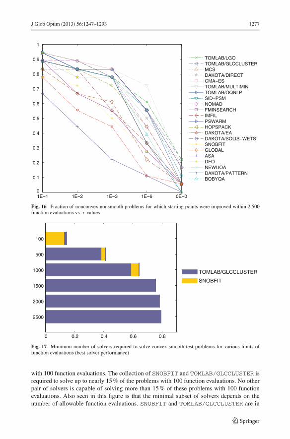
J Glob Optim (2013) 56:1247–1293 1277

1E−1 1E−2 1E−3 1E−6 0E+00

0.1

0.2

0.3

0.4

0.5

0.6

0.7

0.8

0.9

1

TOMLAB/LGOTOMLAB/GLCCLUSTERMCSDAKOTA/DIRECTCMA−ESTOMLAB/MULTIMINTOMLAB/OQNLPSID−PSMNOMADFMINSEARCHIMFILPSWARMHOPSPACKDAKOTA/EADAKOTA/SOLIS−WETSSNOBFITGLOBALASADFONEWUOADAKOTA/PATTERNBOBYQA

Fig. 16 Fraction of nonconvex nonsmooth problems for which starting points were improved within 2,500function evaluations vs. τ values

0 0.2 0.4 0.6 0.8

2500

2000

1500

1000

500

100

TOMLAB/GLCCLUSTER

SNOBFIT

Fig. 17 Minimum number of solvers required to solve convex smooth test problems for various limits offunction evaluations (best solver performance)

with 100 function evaluations. The collection of SNOBFIT and TOMLAB/GLCCLUSTER isrequired to solve up to nearly 15 % of the problems with 100 function evaluations. No otherpair of solvers is capable of solving more than 15 % of these problems with 100 functionevaluations. Also seen in this figure is that the minimal subset of solvers depends on thenumber of allowable function evaluations. SNOBFIT and TOMLAB/GLCCLUSTER are in

123

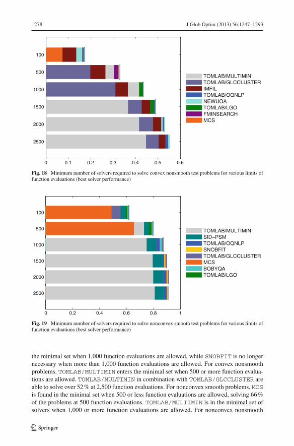
1278 J Glob Optim (2013) 56:1247–1293

0 0.1 0.2 0.3 0.4 0.5 0.6

2500

2000

1500

1000

500

100

TOMLAB/MULTIMINTOMLAB/GLCCLUSTERIMFILTOMLAB/OQNLPNEWUOATOMLAB/LGOFMINSEARCHMCS

Fig. 18 Minimum number of solvers required to solve convex nonsmooth test problems for various limits offunction evaluations (best solver performance)

0 0.2 0.4 0.6 0.8 1

2500

2000

1500

1000

500

100

TOMLAB/MULTIMINSID−PSMTOMLAB/OQNLPSNOBFITTOMLAB/GLCCLUSTERMCSBOBYQATOMLAB/LGO

Fig. 19 Minimum number of solvers required to solve nonconvex smooth test problems for various limits offunction evaluations (best solver performance)

the minimal set when 1,000 function evaluations are allowed, while SNOBFIT is no longernecessary when more than 1,000 function evaluations are allowed. For convex nonsmoothproblems, TOMLAB/MULTIMIN enters the minimal set when 500 or more function evalua-tions are allowed. TOMLAB/MULTIMIN in combination with TOMLAB/GLCCLUSTER areable to solve over 52 % at 2,500 function evaluations. For nonconvex smooth problems, MCSis found in the minimal set when 500 or less function evaluations are allowed, solving 66 %of the problems at 500 function evaluations. TOMLAB/MULTIMIN is in the minimal set ofsolvers when 1,000 or more function evaluations are allowed. For nonconvex nonsmooth

123

J Glob Optim (2013) 56:1247–1293 1279

0 0.1 0.2 0.3 0.4 0.5 0.6

2500

2000

1500

1000

500

100

CMA−ESIMFILTOMLAB/MULTIMINNEWUOATOMLAB/LGONOMAD

Fig. 20 Minimum number of solvers required to solve nonconvex nonsmooth test problems for various limitsof function evaluations (best solver performance)

0 0.2 0.4 0.6 0.8

2500

2000

1500

1000

500

100

TOMLAB/MULTIMINTOMLAB/GLCCLUSTERTOMLAB/OQNLPIMFILSID−PSMSNOBFITTOMLAB/LGOMCSBOBYQANEWUOA

Fig. 21 Minimum number of solvers required to solve all test problems for various limits of function evalu-ations (best solver performance)

problems, NEWUOA, TOMLAB/MULTIMIN, TOMLAB/LGO,and then CMA-ES solved thelargest fraction of problems.

Finally, Fig. 21 shows that TOMLAB/MULTIMIN enters the minimal set of solvers when500 or more function evaluations are allowed. The combination ofTOMLAB/MULTIMIN andTOMLAB/GLCCLUSTER solved the largest fraction of problems over most problem classes.

123

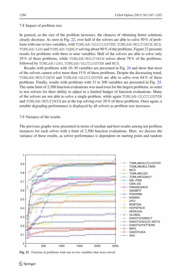
1280 J Glob Optim (2013) 56:1247–1293

7.8 Impact of problem size

In general, as the size of the problem increases, the chances of obtaining better solutionsclearly decrease. As seen in Fig. 22, over half of the solvers are able to solve 50 % of prob-lems with one or two variables, with TOMLAB/GLCCLUSTER, TOMLAB/MULTIMIN, MCS,TOMLAB/LGO andTOMLAB/OQNLP solving about 90 % of the problems. Figure 23 presentsresults for problems with three to nine variables. Half of the solvers are able to solve only29 % of these problems, while TOMLAB/MULTIMIN solves about 78 % of the problems,followed by TOMLAB/LGO, TOMLAB/GLCCLUSTER and MCS.

Results with problems with 10–30 variables are presented in Fig. 24 and show that mostof the solvers cannot solve more than 15 % of these problems. Despite the decreasing trend,TOMLAB/MULTIMIN and TOMLAB/GLCCLUSTER are able to solve over 64 % of theseproblems. Finally, results with problems with 31 to 300 variables are presented in Fig. 25.The same limit of 2,500 function evaluations was used even for the largest problems, in orderto test solvers for their ability to adjust to a limited budget of function evaluations. Manyof the solvers are not able to solve a single problem, while again TOMLAB/GLCCLUSTERand TOMLAB/MULTIMIN are at the top solving over 28 % of these problems. Once again, anotable degrading performance is displayed by all solvers as problem size increases.

7.9 Variance of the results

The previous graphs were presented in terms of median and best results among ten probleminstances for each solver with a limit of 2,500 function evaluations. Here, we discuss thevariance of these results, as solver performance is dependent on starting point and random

0 500 1000 1500 2000 25000

0.1

0.2

0.3

0.4

0.5

0.6

0.7

0.8

0.9

1

TOMLAB/GLCCLUSTERTOMLAB/MULTIMINMCSTOMLAB/LGOTOMLAB/OQNLPSID−PSMCMA−ESFMINSEARCHSNOBFITPSWARMNOMADDFOBOBYQAHOPSPACKNEWUOAGLOBALDAKOTA/DIRECTDAKOTA/SOLIS−WETSDAKOTA/PATTERNIMFILDAKOTA/EAASA

Fig. 22 Fraction of problems with one to two variables that were solved

123

J Glob Optim (2013) 56:1247–1293 1281

0 500 1000 1500 2000 25000

0.1

0.2

0.3

0.4

0.5

0.6

0.7

0.8

TOMLAB/MULTIMINTOMLAB/LGOTOMLAB/GLCCLUSTERMCSTOMLAB/OQNLPSID−PSMCMA−ESSNOBFITBOBYQAFMINSEARCHNOMADNEWUOAPSWARMHOPSPACKDFODAKOTA/DIRECTGLOBALDAKOTA/PATTERNIMFILDAKOTA/SOLIS−WETSDAKOTA/EAASA

Fig. 23 Fraction of problems with three to nine variables that were solved

0 500 1000 1500 2000 25000

0.1

0.2

0.3

0.4

0.5

0.6

0.7

TOMLAB/MULTIMINTOMLAB/GLCCLUSTERTOMLAB/OQNLPMCSTOMLAB/LGOSID−PSMBOBYQANEWUOASNOBFITIMFILHOPSPACKCMA−ESDAKOTA/DIRECTNOMADPSWARMDFODAKOTA/PATTERNGLOBALFMINSEARCHDAKOTA/SOLIS−WETSASADAKOTA/EA

Fig. 24 Fraction of problems with 10–30 variables that were solved

seeds used in the computations. Since the difference in scales of the global solutions and therange of values of the objective function of the test problems prevent a direct comparison,objective function values obtained were scaled as follows:

123

1282 J Glob Optim (2013) 56:1247–1293

0 500 1000 1500 2000 25000

0.05

0.1

0.15

0.2

0.25

0.3

0.35

0.4

TOMLAB/GLCCLUSTERTOMLAB/MULTIMINMCSTOMLAB/OQNLPSNOBFITBOBYQATOMLAB/LGODAKOTA/DIRECTNEWUOAHOPSPACKSID−PSMIMFILCMA−ESASANOMADDFOFMINSEARCHPSWARMDAKOTA/EADAKOTA/PATTERNDAKOTA/SOLIS−WETSGLOBAL

Fig. 25 Fraction of problems with 31–300 variables that were solved

fscaled = 1 − fsolver − fL

fW − fL,

where fsolver is a solution reported by the solver, fL is the global solution, and fW is theworst solution obtained by the solver among the ten runs from different starting points. Theresulting fscaled is in the interval [0, 1] with a value of 1 corresponding to the global solutionand a value of 0 corresponding to the worst solution reported by the solver.

Figure 26 displays the average scaled best, mean, median and worst results among the tenoptimization instances for all test problems. TOMLAB/GLCCLUSTER and TOMLAB/MUL-TIMIN achieve results close to 1 and with low variability among the best, mean, median andworst results. Detailed variability graphs are presented for each solver in the on-line material.

7.10 Impact of missing bounds

As presented in Table 4, a significant number of test problems contain at least one vari-able without lower or upper bounds. Figure 27 presents the fraction of problems solved forproblems grouped by the availability of bounds on their variables. Problems with bounds onall their variables display a much higher percentage of success than the other two classes.Better results are obtained for entirely unbounded problems compared to problems with onlylower bounds available. This is caused by the corresponding problem sizes (see Table 4).CMA-ES, PSWARM, NOMAD and GLOBAL are found to be most sensitive to the absence ofbounds.

7.11 Refinement ability

The following experiment was designed to analyze the ability of solvers to obtain a highlyaccurate solution. The solvers were provided an initial solution close to a global solution of

123

J Glob Optim (2013) 56:1247–1293 1283

0.6

0.65

0.7

0.75

0.8

0.85

0.9

0.95

1

IMF

IL

TO

MLA

B/G

LCC

LUS

TE

R

TO

MLA

B/M

ULT

IMIN

TO

MLA

B/O

QN

LP

MC

S

CM

A−

ES

DA

KO

TA

/SO

LIS

−W

ET

S

PS

WA

RM

NE

WU

OA

DA

KO

TA

/DIR

EC

T

TO

MLA

B/L

GO

GLO

BA

L

SID

−P

SM

BO

BY

QA

HO

PS

PA

CK

SN

OB

FIT

DA

KO

TA

/PA

TT

ER

N

NO

MA

D

FM

INS

EA

RC

H

DA

KO

TA

/EA

AS

A

DF

O

bestmeanmedianworst

Fig. 26 Scaled results for the best, mean, median and worst result among the 10 optimization instances after2,500 function evaluations for each solver

the problem and a feasible space that was asymmetric with respect to the global solution x∗.In particular, the ranges of all variables were set to [−0.166 + x∗, 0.033+ x∗], allowing eachvariable a range of 0.2, unless the original problem bounds were tighter, in which case thelatter were used.

Figure 28 presents the fraction of problems of different size that were solved to withinthe optimality tolerance. It can be noted that for problems with one or two variables, most ofthe solvers are able to find the global solution in over 90 % of the cases. For problems withthree to nine variables, only 8 solvers are able to solve more than 90 % of the cases. TOM-LAB/GLCCLUSTER solves most problems involving ten to thirty variables, with just over71 % of the problems, followed within 5 % by five other solvers. Performance for problemswith over thirty variables drops significantly for all solvers except for TOMLAB/OQNLP,NEWUOA and BOBYQA, which solve around 50 % of the problems. Figs. 29, 30, 31, and 32present similar refinement ability results for each problem class, while the on-line supplementpresents detailed graphs for each solver separately.

7.12 Solution of a test set unseen by developers

In an effort to encourage developers to improve their implementations, the above computa-tional results were shared with developers over several rounds in the course of our study. Thedevelopers of DAKOTA, IMFIL, SID-PSM, and the TOMLAB solvers improved their codes

123

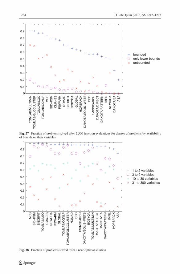
1284 J Glob Optim (2013) 56:1247–1293

0

0.1

0.2

0.3

0.4

0.5

0.6

0.7

0.8

0.9

1

TO

MLA

B/M

ULT

IMIN

TO

MLA

B/G

LCC

LUS

TE

R

TO

MLA

B/L

GO

TO

MLA

B/O

QN

LPM

CS

SID

−P

SM

CM

A−

ES

PS

WA

RM

NO

MA

DS

NO

BF

ITB

OB

YQ

A

GLO

BA

LH

OP

SP

AC

KD

AK

OT

A/S

OLI

S−

WE

TS

DF

OF

MIN

SE

AR

CH

DA

KO

TA

/DIR

EC

T

DA

KO

TA

/PA

TT

ER

NIM

FIL

NE

WU

OA

DA

KO

TA

/EA

AS

A

boundedonly lower boundsunbounded

Fig. 27 Fraction of problems solved after 2,500 function evaluations for classes of problems by availabilityof bounds on their variables

0

0.1

0.2

0.3

0.4

0.5

0.6

0.7

0.8

0.9

1

MC

SS

ID−

PS

M

SN

OB

FIT

TO

MLA

B/L

GO

CM

A−

ES

NE

WU

OA

PS

WA

RM

GLO

BA

LT

OM

LAB

/OQ

NLP

TO

MLA

B/G

LCC

LUS

TE

RN

OM

AD

DF

OF

MIN

SE

AR

CH

DA

KO

TA

/SO

LIS

−W

ET

SB

OB

YQ

AT

OM

LAB

/MU

LTIM

IN

DA

KO

TA

/DIR

EC

TD

AK

OT

A/E

A

DA

KO

TA

/PA

TT

ER

NIM

FIL

HO

PS

PA

CK

AS

A

1 to 2 variables3 to 9 variables10 to 30 variables31 to 300 variables

Fig. 28 Fraction of problems solved from a near-optimal solution

123

J Glob Optim (2013) 56:1247–1293 1285

0

0.1

0.2

0.3

0.4

0.5

0.6

0.7

0.8

0.9

1

DF

ON

EW

UO

AIM

FIL

MC

SH

OP

SP

AC

KD

AK

OT

A/S

OLI

S−

WE

TS

SN

OB

FIT

TO

MLA

B/L

GO

CM

A−

ES

BO

BY

QA

TO

MLA

B/M

ULT

IMIN

TO

MLA

B/O

QN

LPT

OM

LAB

/GLC

CLU

ST

ER

FM

INS

EA

RC

HS

ID−

PS

MP

SW

AR

MD

AK

OT

A/P

AT

TE

RN

NO

MA

DD

AK

OT

A/D

IRE

CT

GLO

BA

LD

AK

OT

A/E

AA

SA

3 to 9 variables10 to 30 variables31 to 300 variables

Fig. 29 Fraction of convex smooth problems solved from a near-optimal solution

0

0.1

0.2

0.3

0.4

0.5

0.6

0.7

0.8

0.9

1

NO

MA

DD

FO

NE

WU

OA

FM

INS

EA

RC

HIM

FIL

MC

SS

ID−

PS

MP

SW

AR

MH

OP

SP

AC

KD

AK

OT

A/D

IRE

CT

DA

KO

TA

/EA

DA

KO

TA

/PA

TT

ER

ND

AK

OT

A/S

OLI

S−

WE

TS

SN

OB

FIT

TO

MLA

B/L

GO

CM

A−

ES

GLO

BA

LT

OM

LAB

/MU

LTIM

INT

OM

LAB

/OQ

NLP

TO

MLA

B/G

LCC

LUS

TE

RB

OB

YQ

AA

SA

1 to 2 variables3 to 9 variables10 to 30 variables31 to 300 variables

Fig. 30 Fraction of convex nonsmooth problems solved from a near-optimal solution

123

1286 J Glob Optim (2013) 56:1247–1293

0

0.1

0.2

0.3

0.4

0.5

0.6

0.7

0.8

0.9

1

MC

SS

ID−

PS

MS

NO

BF

ITT

OM

LAB

/LG

OC

MA

−E

SD

FO

NE

WU

OA

PS

WA

RM

GLO

BA

LB

OB

YQ

AT

OM

LAB

/OQ

NLP

TO

MLA

B/G

LCC

LUS

TE

RN

OM

AD

FM

INS

EA

RC

HD

AK

OT

A/S

OLI

S−

WE

TS

TO

MLA

B/M

ULT

IMIN

DA

KO

TA

/DIR

EC

TD

AK

OT

A/E

AD

AK

OT

A/P

AT

TE

RN

IMF

ILH

OP

SP

AC

KA

SA

1 to 2 variables3 to 9 variables10 to 30 variables31 to 300 variables

Fig. 31 Fraction of nonconvex smooth problems solved from a near-optimal solution

0

0.1

0.2

0.3

0.4

0.5

0.6

0.7

0.8

0.9

1

NO

MA

DN

EW

UO

AF

MIN

SE

AR

CH

MC

SS

ID−

PS

MP

SW

AR

MD

AK

OT

A/D

IRE

CT

DA

KO

TA

/EA

DA

KO

TA

/PA

TT

ER

ND

AK

OT

A/S

OLI

S−

WE

TS

SN

OB

FIT

TO

MLA

B/L

GO

CM

A−

ES

GLO

BA

LB

OB

YQ

AT

OM

LAB

/MU

LTIM

INT

OM

LAB

/OQ

NLP

TO

MLA

B/G

LCC

LUS

TE

RA

SA

DF

OIM

FIL

HO

PS

PA

CK

1 to 2 variables3 to 9 variables10 to 30 variables

Fig. 32 Fraction of nonconvex nonsmooth problems solved from a near-optimal solution

123

J Glob Optim (2013) 56:1247–1293 1287

using feedback from our results. This raises the question whether this process may haveled to overtraining of the software on our test problem collection. To address this question,we solved a set of an additional 502 problems that had never been seen by the developers.These additional test problems were obtained from the original ones via a transformationof variables that preserves smoothness and convexity characteristics but otherwise changesthe problems considerably, including the shape of the objective functions and location of alllocal solutions. In particular, the following linear transformation was used:

x = x + (1 + tu′x)u,

t = (c − 1)/u′u,

where u is a randomly generated vector with elements in [0, 1), and c is the condition numberof the transformation. We chose c = 2, so as to result in a variable space that is of similarsize to that of the original space. The results with and without the transformation were almostidentical.

8 Conclusions

While much work is still to be done, especially for the constrained case, significant progresshas been made on the algorithmic and theoretical aspects of derivative-free optimizationover the past two decades. Without doubt, the most important results from this activity arethe recent model-based algorithms as well as proofs of global convergence for direct andmodel-based approaches.

A set of 22 leading software implementations of state-of-the-art derivative-free optimi-zation algorithms were tested on a large collection of publicly available problems, whosesolutions were obtained using derivative-based and global optimization algorithms. Our com-putational results show that attaining the best solutions even for small problems is a challengefor most current derivative-free solvers. The solvers TOMLAB/MULTIMIN, TOMLAB/GLC-CLUSTER, MCS and TOMLAB/LGO, on average, provide the best solutions among all thesolvers tested. However, computational results show that there is no single solver whoseperformance dominates that of all others. In addition, all solvers provided the best solutionpossible for at least some of the test problems. Although no subset of solvers suffices to solveall problems, our results suggest that the combination of the commercial TOMLAB/MULTI-MIN and TOMLAB/GLCCLUSTER with the free MCS and SNOBFIT is sufficient to providethe best results in most cases. Problem dimensionality and nonsmoothness were found to rap-idly increase the complexity of the search and decrease performance for all solvers. Finally,from a starting point close to a solution, TOMLAB/OQNLP, NEWUOA and TOMLAB/MULTI-MIN showed the fastest convergence towards the solution. Missing bounds on the variablesare found to affect significantly the performance of all solvers, particularly the stochasticones.

The issues of explicit or hidden constraints and noise in the objective function calcula-tion have not been addressed in this paper. These issues are complex and warrant furtherstudy on their own. In this direction, we performed experiments with applications for whichthe objective function was a true black-box that was not available in algebraic form. Theresults from these experiments suggest that the solvers identified as best herein indeed suf-fice to address a variety of true black-box application problems. These results are detailedelsewhere [13,26,43,120,128,139,144].

123

1288 J Glob Optim (2013) 56:1247–1293

Acknowledgments This work was supported over a period of seven years by the Joint NSF/NIGMS Initia-tive to Support Research in the Area of Mathematical Biology under NIH award GM072023, National EnergyTechnology Laboratory’s on-going research in CO2 capture under the RES contract DE-FE-0004000, andthe National Science Foundation under award CBET-1033661. The quality of this paper benefited signifi-cantly from discussions with the authors of the software listed in Table 2. Their constructive comments andsuggestions on several drafts of this paper are far too many to be acknowledged individually.

References

1. Aarts, E.H.L., van Laarhoven, P.J.M.: Statistical cooling: a general approach to combinatorial optimi-zation problems. Phillips J. Res. 40, 193–226 (1985)

2. Abramson, M.A.: Pattern Search Algorithms for Mixed Variable General Constrained OptimizationProblems. PhD thesis, Department of Computational and Applied Mathematics, Rice University, Hous-ton (2002, Aug)

3. Abramson, M.A.: NOMADm Version 4.5 User’s Guide. Air Force Institute of Technology, Wright-Patt-erson AFB, OH (2007)

4. Abramson, M.A., Asaki, T.J., Dennis, J.E. Jr., O’Reilly, K.R., Pingel, R.L.: Quantitative object recon-struction via Abel-based X-ray tomography and mixed variable optimization. SIAM J. Imaging Sci. 1,322–342 (2008)

5. Abramson, M.A., Audet, C.: Convergence of mesh adaptive direct search to second-order stationarypoints. SIAM J. Optim. 17, 606–609 (2006)

6. Abramson, M.A., Audet, C., Couture, G., Dennis, J.E. Jr., LeDigabel, S.: The Nomad project. http://www.gerad.ca/nomad/

7. Abramson, M.A., Audet, C., Dennis, J.E. Jr.: Filter pattern search algorithms for mixed variable con-strained optimization problems. Pac. J. Optim. 3, 477–500 (2007)

8. Abramson, M.A., Audet, C., Dennis, J.E. Jr., Le Digabel, S.: OrthoMADS: a deterministic MADSinstance with orthogonal directions. SIAM J. Optim. 20, 948–966 (2009)

9. Audet, C.: Convergence results for generalized pattern search algorithms are tight. Optim. Eng. 5, 101–122 (2004)

10. Audet, C., Béchard, V., Chaouki, J.: Spent potliner treatment process optimization using a MADS algo-rithm. Optim. Eng. 9, 143–160 (2008)

11. Audet, C., Dennis, J.E. Jr.: Mesh adaptive direct search algorithms for constrained optimization. SIAMJ. Optim. 17, 188–217 (2006)

12. Audet, C., Dennis, J.E. Jr.: A progressive barrier for derivative-free nonlinear programming. SIAM J.Optim. 20, 445–472 (2009)

13. Awasthi, S.: Molecular Docking by Derivative-Free Optimization Solver. Master’s thesis, Departmentof Chemical Engineering, Carnegie Mellon University, Pittsburgh (2008)

14. Barros, P.A. Jr., Kirby, M.R., Mavris, D.N.: Impact of sampling techniques selection on the creation ofresponse surface models. SAE Trans. J. Aerosp. 113, 1682–1693 (2004)

15. Bartholomew-Biggs, M.C., Parkhurst, S.C., Wilson, S.P.: Using DIRECT to solve an aircraft routingproblem. Comput. Optim. Appl. 21, 311–323 (2002)

16. Barton, R.R.: Metamodeling: A state of the art review. In: Proceedings of the 1994 Winter SimulationConference, pp. 237–244 (1994)

17. Bélisle, C.J., Romeijn, H.E., Smith, R.L.: Hit-and-run algorithms for generating multivariate distribu-tions. Math. Oper. Res. 18, 255–266 (1993)

18. Bethke, J.D.: Genetic Algorithms as Function Optimizers. PhD thesis, Department of Computer andCommunication Sciences, University of Michigan, Ann Arbor (1980)

19. Björkman, M., Holmström, K.: Global optimization of costly nonconvex functions using radial basisfunctions. Optim. Eng. 1, 373–397 (2000)

20. Boender, C.G.E., Rinnooy Kan, A.H.G., Timmer, G.T.: A stochastic method for global optimiza-tion. Math. Program. 22, 125–140 (1982)

21. Boneh, A., Golan, A.: Constraints’ redundancy and feasible region boundedness by random feasiblepoint generator (RFPG). In: 3rd European Congress on Operations Research (EURO III), Amsterdam(1979)

22. Booker, A.J., Dennis, J.E., Jr., Frank, P.D., Serafini, D.B., Torczon, V.J., Trosset, M.W.: A rigorousframework for optimization of expensive functions by surrogates. In: ICASE Report, pp. 1–24 (1998)

23. Booker, A.J., Dennis, J.E. Jr., Frank, P.D., Serafini, D.B., Torczon, V.J., Trosset, M.W.: A rigorousframework for optimization of expensive functions by surrogates. Struct. Optim. 17, 1–13 (1999)

123

J Glob Optim (2013) 56:1247–1293 1289

24. Booker, A.J., Meckesheimer, M., Torng, T.: Reliability based design optimization using designexplorer. Optim. Eng. 5, 179–205 (2004)

25. Brent, R.P.: Algorithms for Minimization without Derivatives. Prentice-Hall, Englewood Cliffs (1973)26. Chang, K.-F.: Modeling and Optimization of Polymerase Chain Reaction Using Derivative-Free Opti-

mization. Master’s thesis, Department of Chemical Engineering, Carnegie Mellon University, Pittsburgh(2011)

27. Chiang, T., Chow, Y.: A limit theorem for a class of inhomogeneous Markov processes. Ann. Pro-bab. 17, 1483–1502 (1989)

28. COIN-OR Project. Derivative Free Optimization. http://projects.coin-or.org/Dfo29. COIN-OR Project. IPOPT 2.3.x A software package for large-scale nonlinear optimization. http://

www.coin-or.org/Ipopt/ipopt-fortran.html30. Conn, A.R., Gould, N., Lescrenier, M., Toint, Ph.L.: Performance of a multifrontal scheme for partially

separable optimization. In: Gomez, S., Hennart, J.-P. (eds.) Advances in Optimization and NumericalAnalysis, pp. 79–96. Kluwer, Dordrecht (1994)

31. Conn, A.R., Scheinberg, K., Toint, P.L. : On the convergence of derivative-free methods for uncon-strained optimization. In: Buhmann, M.D., Iserles, A. (eds.) Approximation Theory and Optimization,Tribute to M. J. D. Powell, pp. 83–108. Cambridge University Press, Cambridge (1996)

32. Conn, A.R., Scheinberg, K., Toint, P.L.: Recent progress in unconstrained nonlinear optimization withoutderivatives. Math. Program. 79, 397–414 (1997)

33. Conn, A.R., Scheinberg, K., Toint, P.L.: A derivative free optimization algorithm in practice. In: Pro-ceedings of AIAA St Louis Conference, pp. 1–11 (1998)

34. Conn, A.R., Scheinberg, K., Vicente, L.N.: Global convergence of general derivative-free trust-regionalgorithms to first and second order critical points. SIAM J. Optim. 20, 387–415 (2009)

35. Conn, A.R., Scheinberg, K., Vicente, L.N.: Introduction to derivative-free optimization. SIAM, Phila-delphia (2009)

36. Cox, D.D., John, S.: SDO: A statistical method for global optimization. In: Multidisciplinary DesignOptimization (Hampton, VA, 1995), pp. 315–329. SIAM, Philadelphia (1997)

37. Csendes, T., Pál, L., Sendín, J.O.H., Banga, J.R.: The GLOBAL optimization method revisited. Optim.Lett. 2, 445–454 (2008)

38. Custódio, A.L., Dennis, J.E. Jr., Vicente, L.N.: Using simplex gradients of nonsmooth functions in directsearch methods. IMA J. Numer. Anal. 28, 770–784 (2008)

39. Custódio, A.L., Rocha, H., Vicente, L.N.: Incorporating minimum Frobenius norm models in directsearch. Comput. Optim. Appl. (to appear)

40. Custódio, A.L., Vicente, L.N.: Using sampling and simplex derivatives in pattern search methods. SIAMJ. Optim. 18, 537–555 (2007)

41. Custódio, A.L., Vicente, L.N.: SID-PSM: A Pattern Search Method Guided by Simplex Derivatives forUse in Derivative-Free Optimization. Departamento de Matemática, Universidade de Coimbra, Coimbra(2008)

42. Deming, S.N., Parker, L.R. Jr., Denton, M.B.: A review of simplex optimization in analytical chemis-try. Crit. Rev. Anal. Chem. 7, 187–202 (1974)

43. Desai, R.: A Comparison of Algorithms for Optimizing the Omega Function. Master’s thesis, Departmentof Chemical Engineering, Carnegie Mellon University, Pittsburgh (2010)

44. Eberhart, R.,Kennedy, J.: A new optimizer using particle swarm theory. In: Proceedings of the 6thInternational Symposium on Micro Machine and Human Science, Nagoya, pp. 39–43 (1995)

45. Eldred, M.S., Adams, B.M., Gay, D.M., Swiler, L.P., Haskell, K., Bohnhoff, W.J., Eddy, J.P., Hart, W.E.,Watson, J-P, Hough, P.D., Kolda, T.G., Williams, P.J., Martinez-Canales, M.L., DAKOTA, A.: Multi-level Parallel Object-Oriented Framework for Design Optimization, Parameter Estimation, UncertaintyQuantification, and Sensitivity Analysis: Version 4.2 User’s Manual. Sandia National Laboratories,Albuquerque (2008)

46. Fan, S.S., Zahara, E.: A hybrid simplex search and particle swarm optimization for unconstrained opti-mization. Eur. J. Oper. Res. 181, 527–548 (2007)

47. Finkel, D.E., Kelley, C.T.: Additive scaling and the DIRECT algorithm. J. Glob. Optim. 36, 597–608 (2006)

48. Fowler, K.R., Reese, J.P., Kees, C.E., Dennis, J.E. Jr., Kelley, C.T., Miller, C.T., Audet, C., Booker, A.J.,Couture, G., Darwin, R.W., Farthing, M.W., Finkel, D.E., Gablonsky, J.M., Gray, G., Kolda, T.G.: Acomparison of derivative-free optimization methods for groundwater supply and hydraulic capture com-munity problems. Adv. Water Resour. 31, 743–757 (2008)

49. Gablonsky, J.M.: Modifications of the DIRECT Algorithm. PhD thesis, Department of Mathematics,North Carolina State University, Raleigh (2001)

123

1290 J Glob Optim (2013) 56:1247–1293

50. Gilmore, P., Kelley, C.T.: An implicit filtering algorithm for optimization of functions with many localminima. SIAM J. Optim. 5, 269–285 (1995)

51. GLOBAL Library. http://www.gamsworld.org/global/globallib.htm52. Gray, G., Kolda, T., Sale, K., Young, M.: Optimizing an empirical scoring function for transmembrane

protein structure determination. INFORMS J. Comput. 16, 406–418 (2004)53. Gutmann, H.-M.: A radial basis function method for global optimization. J. Glob. Optim. 19, 201–

227 (2001)54. Han, J., Kokkolaras, M., Papalambros, P.Y.: Optimal design of hybrid fuel cell vehicles. J. Fuel Cell Sci.

Technol. 5, 041014 (2008)55. Hansen, N.: The CMA Evolution Strategy: A tutorial. http://www.lri.fr/hansen/cmaesintro.html56. Hansen, N.: The CMA evolution strategy: a comparing review. In: Lozano, J.A., Larranaga, P., Inza, I.,

Bengoetxea, E. (eds.) Towards a New Evolutionary Computation. Advances on Estimation of Distribu-tion Algorithms, pp. 75–102. Springer, Berlin (2006)

57. Hayes, R.E., Bertrand, F.H., Audet, C., Kolaczkowski, S.T.: Catalytic combustion kinetics: using a directsearch algorithm to evaluate kinetic parameters from light-off curves. Can. J. Chem. Eng. 81, 1192–1199 (2003)

58. Holland, J.H.: Adaptation in Natural and Artificial Systems. The University of Michigan Press, AnnArbor (1975)

59. Holmström, K.: Private Communication (2009)60. Holmström, K., Göran, A.O., Edvall, M.M.: User’s Guide for TOMLAB 7. Tomlab Optimization. http://

tomopt.com61. Holmström, K., Göran, A.O., Edvall, M.M.: User’s Guide for TOMLAB/CGO. Tomlab Optimization

(2007). http://tomopt.com62. Holmström, K., Göran, A.O., Edvall, M.M.: User’s Guide for TOMLAB/OQNLP. Tomlab Optimization

(2007). http://tomopt.com63. Holmström, K., Quttineh, N.-H., Edvall, M.M.: An adaptive radial basis algorithm (ARBF) for expensive

black-box mixed-integer constrained global optimization. Optim. Eng. 9, 311–339 (2008)64. Hooke, R., Jeeves, T.A.: Direct search solution of numerical and statistical problems. J. Assoc. Comput.

Mach. 8, 212–219 (1961)65. Huyer, W., Neumaier, A.: Global optimization by multilevel coordinate search. J. Glob. Optim. 14, 331–

355 (1999)66. Huyer, W., Neumaier, A.: SNOBFIT—Stable noisy optimization by branch and fit. ACM Trans. Math.

Softw. 35, 1–25 (2008)67. Hvattum, L.M., Glover, F.: Finding local optima of high-dimensional functions using direct search

methods. Eur. J. Oper. Res. 195, 31–45 (2009)68. Ingber, L.: Adaptive Simulated Annealing (ASA). http://www.ingber.com/#ASA69. Järvi, T.: A Random Search Optimizer with an Application to a Max–Min Problem. Technical report,

Pulications of the Institute for Applied Mathematics, University of Turku (1973)70. Jones, D.R.: A taxonomy of global optimization methods based on response surfaces. J. Glob. Op-

tim. 21, 345–383 (2001)71. Jones, D.R.: The DIRECT global optimization algorithm. In: Floudas, C.A., Pardalos, P.M. (eds.) Ency-

clopedia of Optimization, vol. 1, pp. 431–440. Kluwer, Boston (2001)72. Jones, D.R., Perttunen, C.D., Stuckman, B.E.: Lipschitzian optimization without the Lipschitz con-

stant. J. Optim. Theory Appl. 79, 157–181 (1993)73. Jones, D.R., Schonlau, M., Welch, W.J.: Efficient global optimization of expensive black-box functions.

J. Glob. Optim. 13, 455–492 (1998)74. Kelley, C.T.: Users Guide for IMFIL version 1.0. http://www4.ncsu.edu/ctk/imfil.html75. Kelley, C.T.: Detection and remediation of stagnation in the Nelder–Mead algorithm using a sufficient

decrease condition. SIAM J. Optim. 10, 43–55 (1999)76. Kelley, C.T.: Iterative Methods for Optimization. SIAM, Philadelphia (1999)77. Kennedy, J., Eberhart, R.: Particle swarm optimization. In: Proceedings of the IEEE International Con-

ference on Neural Networks, Piscataway, pp. 1942–1948 (1995)78. Kirkpatrick, S., Gelatt, C.D., Vecchi, M.P.: Optimization by simulated annealing. Science 220, 671–

680 (1983)79. Kolda, T.G., Lewis, R.M., Torczon, V.J.: Optimization by direct search: new perspectives on some

classical and modern methods. SIAM Rev. 45, 385–482 (2003)80. Kolda, T.G., Torczon, V.J.: On the convergence of asynchronous parallel pattern search. SIAM J.

Optim. 14, 939–964 (2004)81. Lagarias, J.C., Reeds, J.A., Wright, M.H., Wright, P.E.: Convergence properties of the Nelder–Mead

simplex method in low dimensions. SIAM J. Optim. 9, 112–147 (1998)

123

J Glob Optim (2013) 56:1247–1293 1291

82. LeDigabel, S.: NOMAD User Guide Version 3.3. Technical report, Les Cahiers du GERAD (2009)83. Lewis, R.M., Torczon, V.J.: Pattern search algorithms for bound constrained minimization. SIAM J.

Optim. 9, 1082–1099 (1999)84. Lewis, R.M., Torczon, V.J.: Pattern search algorithms for linearly constrained minimization. SIAM J.

Optim. 10, 917–941 (2000)85. Lewis, R.M., Torczon, V.J.: A globally convergent augmented lagrangian pattern search algorithm for

optimization with general constraints and simple bounds. SIAM J. Optim. 12, 1075–1089 (2002)86. Liepins, G.E., Hilliard, M.R.: Genetic algorithms: foundations and applications. Ann. Oper. Res. 21,

31–58 (1989)87. Lin, Y., Schrage, L.: The global solver in the LINDO API. Optim. Methods Softw. 24, 657–668 (2009)88. Lucidi, S., Sciandrone, M.: On the global convergence of derivative-free methods for unconstrained

minimization. SIAM J. Optim. 13, 97–116 (2002)89. Lukšan, L., Vlcek, J.: Test Problems for Nonsmooth Unconstrained and Linearly Constrained Optimi-

zation. Technical report, Institute of Computer Science, Academy of Sciences of the Czech Republic(2000). http://www3.cs.cas.cz/ics/reports/v798-00.ps

90. Marsden, A.L., Feinstein, J.A., Taylor, C.A.: A computational framework for derivative-free optimiza-tion of cardiovascular geometries. Comput. Methods Appl. Mech. Eng. 197, 1890–1905 (2008)

91. Marsden, A.L., Wang, M., Dennis, J.E. Jr., Moin, P.: Optimal aeroacustic shape design using the surrogatemanagement framework. Optim. Eng. 5, 235–262 (2004)

92. Marsden, A.L., Wang, M., Dennis, J.E. Jr., Moin, P.: Trailing-edge noise reduction using derivative-freeoptimization and large-eddy simulation. J. Fluid Mech. 5, 235–262 (2007)

93. Matheron, G.: Principles of geostatistics. Econ. Geol. 58, 1246–1266 (1967)94. McKinnon, K.I.M.: Convergence of the Nelder–Mead simplex method to a nonstationary point. SIAM

J. Optim. 9, 148–158 (1998)95. Metropolis, N., Rosenbluth, A.W., Rosenbluth, M.N., Teller, A.H., Teller, E.: Equation of state calcula-

tions by fast computing machines. J. Chem. Phys. 21, 1087–1092 (1953)96. Mongeau, M., Karsenty, H., Rouzé, V., Hiriart-Urruty, J.B.: Comparison of public-domain software for

black box global optimization. Optim. Methods Softw. 13, 203–226 (2000)97. Moré, J., Wild, S.: Benchmarking derivative-free optimization algorithms. SIAM J. Optim. 20, 172–191

(2009)98. Mugunthan, P., Shoemaker, C.A., Regis, R.G.: Comparison of function approximation, heuristic, and

derivative-based methods for automatic calibration of computationally expensive groundwater bioreme-diation models. Water Resour. Res. 41, W11427 (2005)

99. Nelder, J.A., Mead, R.: A simplex method for function minimization. Comput. J. 7, 308–313 (1965)100. Nesterov, Y.: Gradient methods for minimizing composite objective function. CORE Discussion Paper

2007/76 (2007)101. Neumaier, A.: MCS: Global Optimization by Multilevel Coordinate Search. http://www.mat.univie.ac.

at/neum/software/mcs/102. Neumaier, A., Shcherbina, O., Huyer, W., Vinkó, T.: A comparison of complete global optimization

solvers. Math. Program. 103, 335–356 (2005)103. Oeuvray, R.: Trust-Region Methods Based on Radial Basis Functions with Application to Biomedical

Imaging. PhD thesis, Institute of Mathematics, Swiss Federal Institute of Technology, Lausanne (2005,March)

104. Orosz, J.E., Jacobson, S.H.: Finite-time performance analysis of static simulated annealing algo-rithms. Comput. Optim. Appl. 21, 21–53 (2002)

105. Pintér, J.: Homepage of Pintér Consulting Services. http://www.pinterconsulting.com/106. Pintér, J.D.: Global Optimization in Action: Continuous and Lipschitz Optimization. Algorithms, Imple-

mentations and Applications. Nonconvex Optimization and its Applications. Kluwer, Dordrecht (1995)107. Pintér, J.D., Holmström, K., Göran, A.O., Edvall, M.M.: User’s Guide for TOMLAB/LGO. Tomlab

Optimization (2006). http://tomopt.com108. Plantenga, T.D.: HOPSPACK 2.0 User Manual. Technical Report SAND2009-6265, Sandia National

Laboratories, Albuquerque (2009)109. Powell, M.J.D.: A direct search optimization method that models the objective and constraint functions

by linear interpolation. In: Gomez, S., Hennart, J-P. (eds.) Advances in Optimization and NumericalAnalysis, pp. 51–67. Kluwer, Dordrecht (1994)

110. Powell, M.J.D.: A direct search optimization method that models the objective by quadratic interpolation.In: Presentation at the 5th Stockholm Optimization Days (1994)

111. Powell, M.J.D.: Recent Research at Cambridge on Radial Basis Functions. Technical report, Departmentof Applied Mathematics and Theoretical Physics, University of Cambridge (1998)

123

1292 J Glob Optim (2013) 56:1247–1293

112. Powell, M.J.D.: UOBYQA: unconstrained optimization by quadratic approximation. Math. Pro-gram. 92, 555–582 (2002)

113. Powell, M.J.D.: The NEWUOA software for unconstrained optimization without derivatives. In: Di Pillo,G., Roma, M. Large-Scale Nonlinear Optimization, pp. 255–297. Springer, New York (2006)

114. Powell, M.J.D.: Developments of NEWUOA for minimization without derivatives. IMA J. Numer.Anal. 28, 649–664 (2008)

115. Powell, M.J.D.: The BOBYQA Algorithm for Bound Constrained Optimization Without Derivatives.Technical report, Department of Applied Mathematics and Theoretical Physics, University of Cambridge(2009)

116. Princeton Library. http://www.gamsworld.org/performance/princetonlib/princetonlib.htm117. Regis, R.G., Shoemaker, C.A.: Constrained global optimization of expensive black box functions using

radial basis functions. J. Glob. Optim. 31, 153–171 (2005)118. Regis, R.G., Shoemaker, C.A.: Improved strategies for radial basis function methods for global optimi-

zation. J. Glob. Optim. 37, 113–135 (2007)119. Richtarik, P.: Improved algorithms for convex minimization in relative scale. SIAM J. Optim. (2010, to

appear). http://www.optimization-online.org/DB_FILE/2009/02/2226.pdf120. Rios, L.M.: Algorithms for Derivative-Free Optimization. PhD thesis, Department of Industrial and

Enterprise Systems Engineering, University of Illinois, Urbana (2009, May)121. Romeo, F., Sangiovanni-Vincentelli, A.: A theoretical framework for simulated annealing. Algorithmi-

ca 6, 302–345 (1991)122. Sacks, J., Welch, W.J., Mitchell, T.J., Wynn, H.P.: Design and analysis of computer experiments. Stat.

Sci. 4, 409–423 (1989)123. Sahinidis, N.V., Tawarmalani, M.: BARON 7.5: Global Optimization of Mixed-Integer Nonlinear Pro-

grams, User’s Manual (2005)124. Sandia National Laboratories: The Coliny Project. https://software.sandia.gov/trac/acro/wiki/Overview/

Projects125. Scheinberg, K.: Manual for Fortran Software Package DFO v2.0 (2003)126. Schonlau, M.: Computer Experiments and Global Optimization. PhD thesis, Department of Statistics,

University of Waterloo, Waterloo (1997)127. Serafini, D.B.: A Framework for Managing Models in Nonlinear Optimization of Computationally

Expensive Functions. PhD thesis, Department of Computational and Applied Mathematics, Rice Uni-versity, Houston (1998, Nov)

128. Shah, S.B., Sahinidis, N.V.: SAS-Pro: Simultaneous residue assignment and structure superposition forprotein structure alignment. PLoS ONE 7(5), e37493 (2012)

129. Shubert, B.O.: A sequential method seeking the global maximum of a function. SIAM J. Numer.Anal. 9, 379–388 (1972)

130. Smith, R.L.: Efficient Monte Carlo procedures for generating points uniformly distributed over boundedregions. Oper. Res. 32, 1296–1308 (1984)

131. Søndergaard, J.: Optimization Using Surrogate Models—by the Space Mapping Technique. PhD thesis,Technical University of Denmark, Department of Mathematical Modelling, Lingby (2003)

132. Spendley, W., Hext, G.R., Himsworth, F.R.: Sequential application for simplex designs in optimisationand evolutionary operation. Technometrics 4, 441–461 (1962)

133. Tawarmalani, M., Sahinidis, N.V.: A polyhedral branch-and-cut approach to global optimization. Math.Program. 103, 225–249 (2005)

134. Torczon, V.J.: On the convergence of multidirectional search algorithms. SIAM J. Optim. 1, 123–145 (1991)

135. Torczon, V.J.: On the convergence of pattern search algorithms. SIAM J. Optim. 7, 1–25 (1997)136. Tseng, P.: Fortified-descent simplicial search method: a general approach. SIAM J. Optim. 10, 269–

288 (1999)137. Vaz, A.I.F.: PSwarm Home Page. http://www.norg.uminho.pt/aivaz/pswarm/138. Vaz, A.I.F., Vicente, L.N.: A particle swarm pattern search method for bound constrained global opti-

mization. J. Glob. Optim. 39, 197–219 (2007)139. Wang, H.: Application of Derivative-Free Algorithms in Powder Diffraction. Master’s thesis, Department

of Chemical Engineering, Carnegie Mellon University, Pittsburgh (2011)140. Wild, S.M., Regis, R.G., Shoemaker, C.A.: ORBIT: Optimization by radial basis function interpolation

in trust-regions. SIAM J. Sci. Comput. 30, 3197–3219 (2008)141. Winfield, D.: Function and Functional Optimization by Interpolation in Data Tables. PhD thesis, Harvard

University, Cambridge (1969)

123

J Glob Optim (2013) 56:1247–1293 1293

142. Winslow, T.A., Trew, R.J., Gilmore, P., Kelley, C.T.: Simulated performance optimization of gaas mesfetamplifiers. In: IEEE/Cornell Conference on Advanced Concepts in High Speed Semiconductor Devicesand Circuits, Piscataway, pp. 393–402 (1991)

143. Zhao, Z., Meza, J.C., Van Hove, M.: Using pattern search methods for surface structure determinationof nanomaterials. J. Phys. Condens. Matter 18, 8693–8706 (2006)

144. Zheng, Y.: Pairs Trading and Portfolio Optimization. Master’s thesis, Department of Chemical Engi-neering, Carnegie Mellon University, Pittsburgh (2011)

123