Derivative-Based Fuzzy System Optimization

Dan SimonCleveland State University

1

Suppose we have a fuzzy controller that operates for N time steps. The controller error can be measured as:

2

2

1

1

2

ˆ

ˆ system output at -th time step

desired output at -th time step

N

qq

q q q

q

q

E EN

E y y

y q

y q

Input Modal Points cij

3

2

1

1

2

ˆ

N

qq

q q q

E EN

E y y

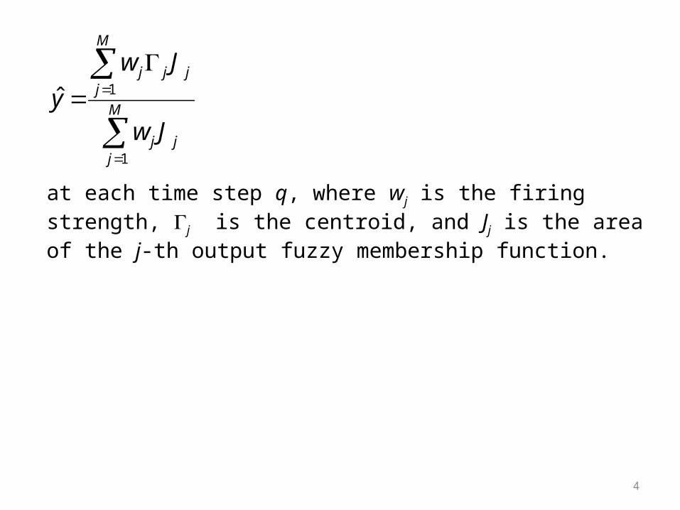
Note that yq is constant. Therefore,

1

ˆ1 Nq

qqij ij

yEE

c N c

at each time step q, where wj is the firing strength, j is the centroid, and Jj is the area of the j-th output fuzzy membership function.

4

1

1

ˆ

M

j j jj

M

j jj

w J

yw J

5

1

1

1 1

2

1

1

ˆ1

ˆ ˆ

ˆ

ˆ( )

Nq

qqij ij

Mq q k

kij k ij

M M

k k j j k j j jq j j

Mk

j jj

k k q

M

j jj

yEE

c N c

y y w

c w c

J w J J w Jy

ww J

J y

w J

1

1

ˆ

M

j j jj

M

j jj

w J

yw J

Definition:ri1k = 1 if x1 fuzzy set i is a premise of the k-th rule and wk = fi1(x1), and ri1k = 0 otherwise. In other words, ri1k = 1 if x1 determines the activation level of the kth rule because of its membership in the i-th fuzzy set.Similarly, ri2k = 1 if x2 fuzzy set i is a premise of the k-th rule and wk = fi2(x2), and ri2k = 0 otherwise.

6

x1 NS (0.8) and x1 Z (0.2)x2 Z (0.3) and x2 PS (0.7)12-th rule: x1 NS and x2 PS y NSTherefore, r2,1,12 = 1.

7

NL NS Z PS PL

NL NL NL NS NS NS

NS NL NS Z Z Z

Z NL NS Z PS PL

PS Z Z Z PS PL

PL PS PS PS PL PL

Change in Error x2

Error x1

Throttle Position Change y

-6 -4 -2 0 2 4 60

0.2

0.4

0.6

0.8

1

Le

ve

l of M

em

be

rsh

ip

Input 1

x1

-6 -4 -2 0 2 4 60

0.2

0.4

0.6

0.8

1

Le

ve

l of M

em

be

rsh

ip

Input 2

x2

Example:

ri,1,12 = 0 for i {1, 3, 4, 5}, and ri,2,12 = 0 for i [1, 5].

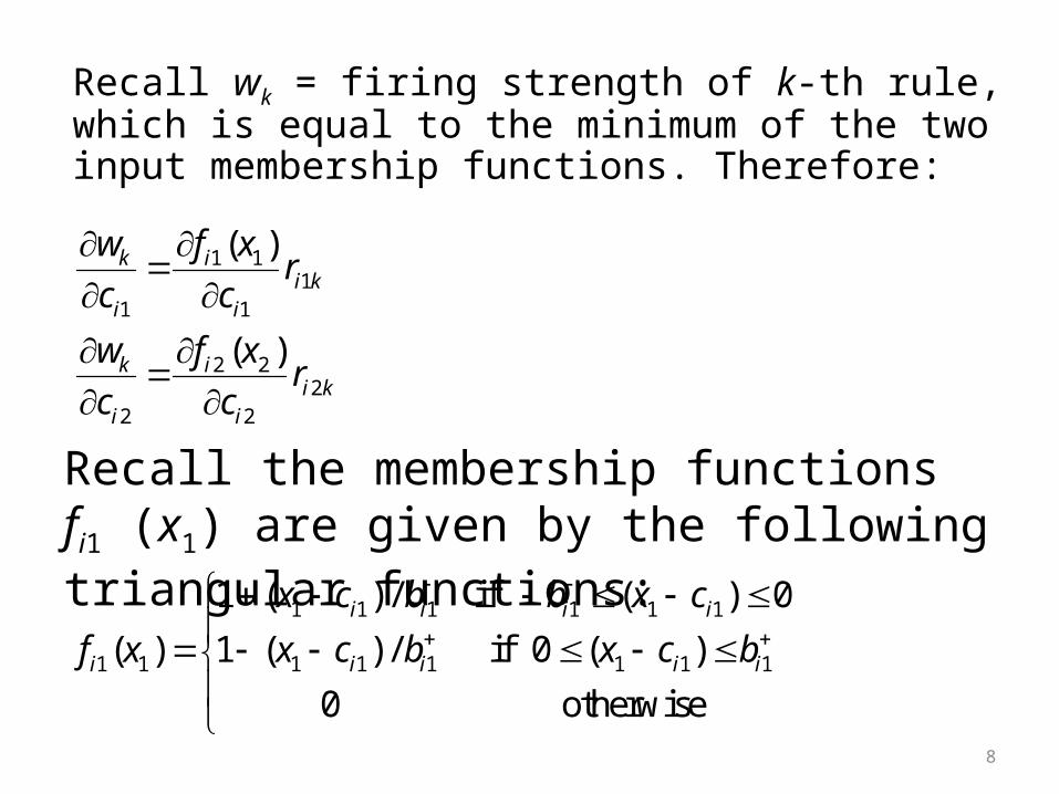
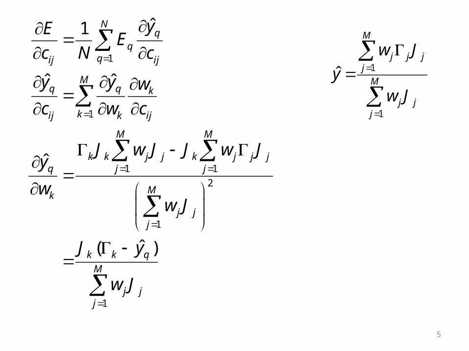
Recall wk = firing strength of k-th rule, which is equal to the minimum of the two input membership functions. Therefore:

8

1 11

1 1

2 22

2 2

( )

( )

k ii k

i i

k ii k

i i

w f xr

c c

w f xr

c c

1 1

1

1 1 1 1

1 1 1 1 11 1

1 ( ) / if ( ) 0

( ) 1 ( ) / if 0 ( )

0 otherwise

ii i

i

i

iiii

x c b b x c

f x x c b x c b

Recall the membership functions fi1 (x1) are given by the following triangular functions:

9

1 1 1 1 1

1 11 1 1 1 1

1

2 2 2 2 2

2 22 2 2 2 2

2

1/ if ( )

1/ if

0 otherwise

1/ if ( )

1/ if

0 otherwise

i i i i

ii i i i

i

i i i i

ii i i i

i

b c b x cf x

b c x c bc

b c b x cf x

b c x c bc

Summary:• The expressions on pages 3, 5, 8, and 9, give us

the partial derivative of the error with respect to the modal points of the input MFs.

• Similar methods are used to find the derivatives of the error with respect to input MF half-widths, output MF modal points, and output MF half-widths.

• Now we can use gradient descent (or another gradient-based method) to optimize the MFs.

Reference: D. Simon, "Sum normal optimization of fuzzy membership functions," International Journal of Uncertainty, Fuzziness and Knowledge-Based Systems, Aug. 2002.

10

Example: Fuzzy Cruise Control – VehicleGrad.m

11

0 20 40 60 80 1000.005

0.01

0.015

0.02

0.025

iterations

err

or

74% error decrease

Performance of cruise control after gradient descent optimization of MFs

12

0 5 10 1539.2

39.4

39.6

39.8

40

40.2

40.4

40.6

Time (sec)

Ve

loci

ty (

me

ters

/se

c)

DefaultOptimized

13-0.5 0 0.50

0.2

0.4

0.6

0.8

1m

em

be

rsh

ip le

vel

Output 1

-0.5 0 0.50

0.2

0.4

0.6

0.8

1

me

mb

ers

hip

leve

l

Output 1

Default Output MFs

Optimized Output MFsPlotMem('paramgu.txt', 2, [5 5], 1, 5)

Throttle change (rad)

The input MFs do not change as much as the output MFs

Some issues to think about:• Why use 5 membership functions for the

output and for each input?• How can we make the response less

oscillatory? How about something like:

where is a weighting parameter

14

2 21

1

1ˆ ˆ)( )(1

2

N

q q qq

E E y yN

• Try different initial conditions (initial fuzzy membership functions)

• Try different gradient descent options• Try different MF shapes• How can we optimize while constraining the

MFs to be sum normal?

15

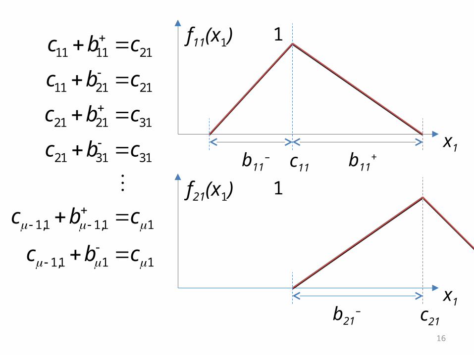
f11(x1)

16

11 11 21

11 21 21

21 21 31

21 31 31

1,1 1,1 1

1,1 1 1

c b c

c b c

c b c

c b c

c b c

c b c

c11b11

–

1

x1b11

+

f21(x1)

c21b21–

1

x1

= number of input 1 fuzzy sets = number of input 2 fuzzy sets = number of output fuzzy sets

17

11 11 11 1 1 1

12 12 12 2 2 2

1 1 1

T

x b b c b b c

b b c b b c

Similar equality constraints can be written for the input 2 MFs, and for the output MFs.

Similar equality constraints for the input 2 MFs and the output MFs

18

1 2 3

1 2 2 3 2 3

2 3 1 2 2 3

2 3 2 3 1 2

1

2

0

d , , )

0 0

0 0

0 0

0 1 1

0 0 1

iag

0 0 1

1 0 1

(

i

L L

M M

M ML

M M

M

Lx

L L

M

L1: 2( 1) 3L2: 2( 1) 3L3: 2( 1) 3

In our case, = 0

19

1 1 1

ˆ ˆmin ( ) ( ) such that

ˆ comes from unconstrained minimization

ˆ ˆ( ) ( )

positive definite we

Solu

ighting matri

ti n:

x

o

Tx

T T

x x W x x Lx

x

x x W L LW L Lx

W

20

0 20 40 60 80 1000.006

0.008

0.01

0.012

0.014

0.016

0.018

0.02

0.022

iterations

err

or

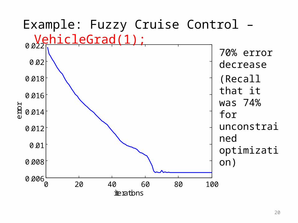
Example: Fuzzy Cruise Control – VehicleGrad(1);

70% error decrease(Recall that it was 74% for unconstrained optimization)

21

0 5 10 1539.2

39.4

39.6

39.8

40

40.2

40.4

40.6

Time (sec)

Ve

loci

ty (

me

ters

/se

c)

DefaultUnconstrained OptimizedConstrained Optimized

Performance of cruise control after unconstrained and constrained gradient descent optimization of MFs

22

-0.5 0 0.50

0.2

0.4

0.6

0.8

1

me

mb

ers

hip

leve

l

Output 1

Default Output MFs

Optimized Constrained Output MFsPlotMem('paramgc.txt', 2, [5 5], 1, 5)

Throttle change (rad)

The input MFs do not change as much as the output MFs

-0.5 0 0.50

0.2

0.4

0.6

0.8

1m

em

be

rsh

ip le

vel

Output 1

Other gradient descent optimization algorithms:• Chapter 3, “A Course in Fuzzy Systems and

Control,” by Li-Xin Wang

23