Derivation of Diagnostic Models Based on Formalized Process Knowledge

Esteban Arroyo*. Denis Schulze*. Lars Christiansen*. Alexander Fay*. Nina F. Thornhill**

*Automation Technology Institute, Helmut Schmidt University, Hamburg, 22043

Germany (e-mail: {e.arroyo, alexander.fay}@hsu-hh.de). **Centre for Process Systems Engineering, Imperial College London, London, SW7 2AZ

United Kingdom (e-mail:n.thornhill@imperial.ac.uk)

Abstract: Industrial systems are vulnerable to faults. Early and accurate detection and diagnosis in production systems can minimize down-time, increase the safety of the plant operation, and reduce manufacturing costs. Knowledge- and model-based approaches to automated fault detection and diagnosis have been demonstrated to be suitable for fault cause analysis within a broad range of industrial processes and research case studies. However, the implementation of these methods demands a complex and error-prone development phase, especially due to the extensive efforts required during the derivation of models and their respective validation. In an effort to reduce such modeling complexity, this paper presents a structured causal modeling approach to supporting the derivation of diagnostic models based on formalized process knowledge. The method described herein exploits the Formalized Process Description Guideline VDI/VDE 3682 to establish causal relations among key-process variables, develops an extension of the Signed Digraph model combined with the use of fuzzy set theory to allow more accurate causality descriptions, and proposes a representation of the resulting diagnostic model in CAEX/AutomationML targeting dynamic data access, portability, and seamless information exchange.

Keywords: Process, knowledge representation, model, fuzzy inference, diagnosis, information exchange.

1. INTRODUCTION

Automated Fault Detection and Diagnosis (AFDD) has acquired an increasing role in modern production facilities where complex interactions between components and control structures make the manual fault analysis highly complex. In such industrial scenarios, the fault of a single component might cause the malfunctioning of the whole system and result in severe consequences in terms of product quality loss, human safety, and economic costs. This fact has led to a surge of academic and industrial effort concentrated on developing effective process monitoring systems (Chiang et al., 2001). As a result, knowledge-based and model-based methods have arisen among current promising approaches to AFDD proving to be suitable for root cause analysis within a broad range of industrial applications (e.g. Ahn et al., 2008, and Lü et al., 2011).

An important model-based approach based on the use of process causality is Signed Directed Graphs (SDGs). Although this approach is characterized for its suitability to describe process connectivity and behavior, some shortcomings such as difficulties in dealing with multiple fault diagnosis and transient responses have limited its industrial application. Accordingly, in an effort to overcome such drawbacks, significant research has been conducted in the field of SDG-based diagnosis in conjunction with alternative methods. Gao et al., (2009), for instance, proposed a monitoring algorithm in which SGDs are combined with real-time bidirectional inference and fuzzy logic. In their work, fuzzy sets are utilized to determine the state of the

nodes within the SDG model and to sort causal priorities, whereas bidirectional inverse inference is employed to cope with compensatory responses. A similar approach combining SGDs and fuzzy set theory for prioritizing root cause candidates and estimating diagnosis confidence was previously introduced by Han et al., (1994). In the same direction, Zhang et al., (2005) developed a diagnosis approach exploiting fuzzy-SDG for patterns identification and diagnosis resolution enhancement, and Shih et al., (1995) propounded a fuzzy-based diagnostic model termed fuzzy cause-effect graph.

Concerning formal process description for AFDD, Christiansen, et al., (2011) discussed the limitations of structural knowledge for fault diagnosis, and proposed the addition of formalized process knowledge in accordance to VDI/VDE 3682 (VDI, 2005). Diagnostic benefits of the combined method are theoretically shown for a chemical mixing process. This approach, however, is limited to causalities of type products-processes-resources and does not deal with causal relations between key-process variables. In the phase of process design, Ulrich, (2009) proposed the use of an extended formalized process description for modeling process within production plants. The propounded extension consists in the addition of a new information element to the VDI/VDE 3682´s classes aimed at the description of information paths within the process.

Most of the aforementioned approaches are focused on the development of diagnosis algorithms and not on the formal generation of causal models on which AFDD algorithms are

Preprints of the 19th World CongressThe International Federation of Automatic ControlCape Town, South Africa. August 24-29, 2014

Copyright © 2014 IFAC 3456

to operate. The rest of them do not delve into detailed causal relations or specifications for models generation. Noting, however, that the success of the diagnosis tasks strictly depends upon the correctness and consistency of the causal model, it is useful to concentrate efforts on the development of methods for effective and accurate model generation. With such a motivation, this paper presents a new modeling approach based on formalized process descriptions. In it, process knowledge is formally structured in accordance to the VDI/VDE 3682 guideline, and further mapped into an extended SDG model (xSDG) in which the values of the arcs are consistently defined by using fuzzy set theory. The subsequent causal graph is transferred to a CAEX/AutomationML file for further dynamic data access and seamless information exchange. This contribution is not intended to introduce a diagnostic algorithm itself, but rather a formal approach to generation of causal models and their representation in a portable and object oriented (OO) format. The resulting model can then be shared with others who might use it for a variety of purposes such as plant AFDD and design of control structures.

The rest of this paper is organized as follows: Section 2 introduces the topic of engineering process description and information exchange presenting for this the Formalized Process Description guideline VDI/VDE 3682, the Computer Aided Exchange Format CAEX, and the engineering data exchange format AutomationML. Section 3 is dedicated to discuss causal modeling based on Signed Digraphs (SDGs), the specification of the eXtended Signed Digraphs (xSDGs) developed herein, and the use of fuzzy set theory for the definition of consistent arc values. The overall method for the generation of the diagnostic model is addressed in Section 4, whereas Section 5 deals with the implementation of the resulting model on CAEX/AutomationML. A case study of a continuous stirred tank heater aimed at exemplifying the application of the method is presented in Section 6, and at last, Section 7 rounds up the paper with the conclusions.

2. ENGINEERING PROCESS DESCRIPTION AND INFORMATION EXCHANGE

2.1 Formalized Process Description (FPD) VDI/VDE 3682

The guideline VDI/VDE 3682 Formalized Process Description (VDI, 2005) allows OO and domain-independent modeling of process information. It establishes seven types of elements, namely: process operator (O), technical resource (T) product (P), energy (E), flow (F), utilization (U) and system boundary (S). Fig. 1 presents a graphic overview of the FPD objects, whereas a model class diagram is depicted in Fig. 2.

Aiming at detailed process descriptions, the guideline also specifies an information model which comprises relations (e.g., aggregation, association, and cardinality) and attributes (i.e., identifier and characteristics). Each operator or state contains an identifier and several characteristics which may be used to describe the nature of these objects in more detail. The reader is referred to Section 2.2 of the guideline for further provisions on the FPD information model.

Fig. 1. Graphic symbols of the guideline VDI/VDE 3682

Fig. 2. Class diagram of a process and its objects (VDI, 2005)

Even though the VDI/VDE 3682 guideline is suitable for describing process sequences and functional relations, the guideline itself does not address the modeling of information structures (e.g. control loops) which are fundamental during fault analysis. Therefore, in order to cope with such a shortcoming, extensions of the guideline have been previously propounded. Ulrich, (2009), for instance, developed an information add-on which allows for the representation of information flow and its causal relation to process variables. His proposal for the graphical representation of the information element is a blue-colored hexagon (I), as shown in the extended formalized process description of Fig. 3. In this example, two products {P1, P2} are mixed in a process O1 which utilizes the resource T1 to generate the product P3 and liberate an energy amount E1. Here, the information element I1 is used to indicate that certain information of the process O1 is used within processes {O2, O3} to control the flow of products {P1, P2} by using resources {T2, T3}.

Fig. 3. Formal process description with information extension

19th IFAC World CongressCape Town, South Africa. August 24-29, 2014

3457

2.2 Computer Aided Engineering Exchange (CAEX)

IEC 62424 defines CAEX as a meta-model for the storage and exchange of engineering models. It comprises the following main components which are the base for the description of the diagnostic model derived in this work:

• InstanceHierarchy (IH): Description of a specific containment hierarchy of components from top-level plant down to single components (InternalElements, IEs) with interfaces (ExternalInterfaces, EIs) and relations (InternalLinks, ILs).

• SystemUnitClass Library: Reusable SystemUnitClasses (SUCs) defining component types down to their respective technical realizations normally organized in vendor-specific product catalogues.

• RoleClass Library: Reusable role classes (RCs) for abstract descriptions of component requirements.

• InterfaceClass Library: Reusable InterfaceClasses (ICs) for specifying connection points of RCs, SUCs, and the interface type of EIs.

• Attributes: Properties for describing characteristics of each previously introduced modeling element.

2.3 AutomationML (AML)

AutomationML is an XML schema-based data format designed for the vendor independent exchange of plant engineering information (AutomationML, 2010). AML stores engineering data following the OO paradigm and accordingly supports features such as re-use and inheritance. It allows representation of a wide variety of plant topology-based models encapsulating different functional aspects, and virtually supports the representation of any model that may be described as a graph.

The core of AML is the top-level data format CAEX but it also allows the integration of external engineering data. The schema has been designed to support references to other exchange data formats such as COLLADA (geometry and kinematics), and PLCopen XML (programmable logic control). Within this work, model descriptions are fully implemented in the base CAEX/AML, and accordingly external referencing is not required.

3. CAUSAL MODELLING

3.1 Signed Digraphs (SDGs)

An SDG is a qualitative model approach to fault diagnosis that incorporates causal analysis to represent process behavior. It is a diagram reflecting causal associations between process parameters by means of nodes and directed arcs. In general, nodes can represent process parameters such as physical variables, sensors, system faults, component failures, or subsystem failures (Chiang et al., 2001), whereas directed arcs represent causal relationships between nodes. A node can take values normal “0”, high “+”, or low “-” which represent its qualitative state. In turn, directed arcs assume values “-” and “+” representing a direct or inverse relationship between the cause and effect nodes. Fig. 4 depicts the basic topology of an SDG.

Fig.4. SDG segment of a chemical reaction process

The fundamental premise of digraph techniques is that cause and effect linkages must connect the fault origin to the observed symptoms of the identified fault (Kramer et al., 1987). Accordingly, during diagnosis measured deviations are propagated from the effect node to the cause nodes through consistent arcs until the root node is identified (Chiang et al., 2001).

3.1.1 SDG formal definition

As a causal graph, an SDG can be formalized as follows: let G= (V,E,Ʌ,Δ) be a graph defined by two non-empty sets namely, the vertex set V (nodes) and the edge set E (directed arcs), with E ⊆V x V, such that Ʌ:E→{+,-} represent the forward influences (values) of the edges, and Δ: V→{+,0,-} the qualitative status of a vertex as follows:

ε "0"

ε " "

ε " "

Where is the set point (steady-state value), and ε is a given threshold.

3.1.2 Arc Consistency in SDGs

An arc of an SDG is said to be consistent if the product of the cause node, the directed arc, and the effect node is positive, i.e. • Ʌ • = “+”. In general, it can be regarded that only consistent arcs can propagate disturbances; however, an exception applies for nodes representing process controlled variables (see Subsection 3.2).

The consistency of an arc can be validated by means of different statistical methods. Yang et al., (2012) introduced causal model validation by using cross-correlation and transfer entropy. Chang et al., (1990) proposed the use of truth tables, and modular SDGs to describe the transition states of the system, and addresses the non-single-transition problem (i.e. arcs changing sign during transients) by introducing a method based on description of variables in velocity-forms. In this contribution, instead, we propose a fuzzy-based approach alongside the use of process historical data and simulation results to establish edge consistency. This method is particularly suitable to deal with uncertainties and demands less computational resources.

3.1.3 SDGs Simplification

In case of finding several consecutive unmeasured nodes within the SDG (i.e. nodes representing unmeasured process

19th IFAC World CongressCape Town, South Africa. August 24-29, 2014

3458

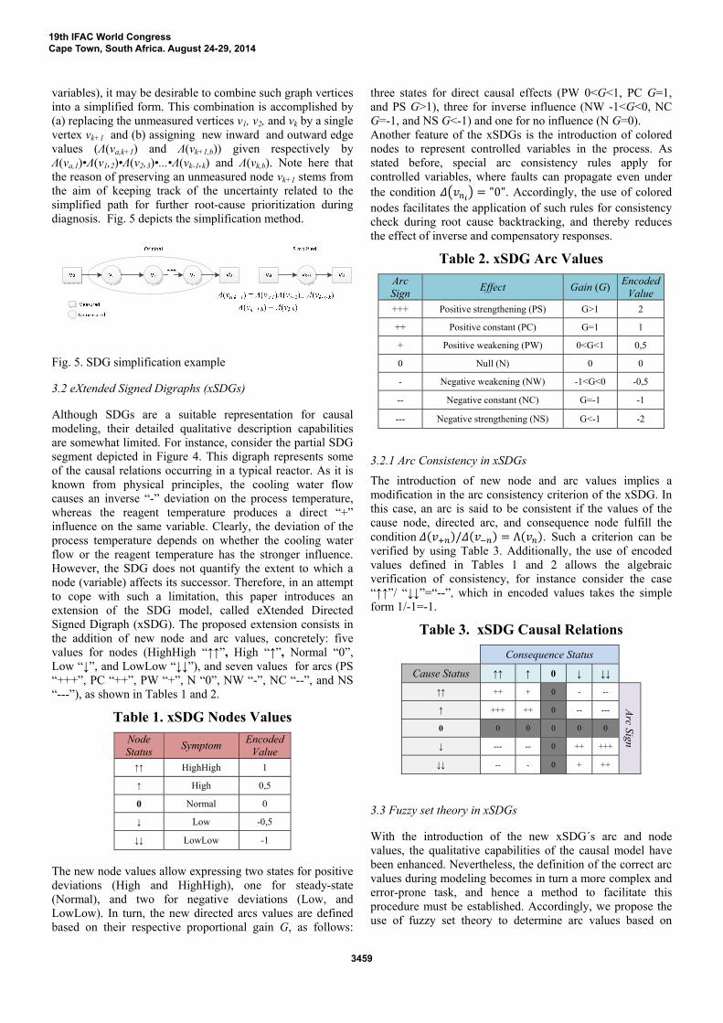
variables), it may be desirable to combine such graph vertices into a simplified form. This combination is accomplished by (a) replacing the unmeasured vertices v1, v2, and vk by a single vertex vk+1 and (b) assigning new inward and outward edge values (Ʌ(va,k+1) and Ʌ(vk+1,b)) given respectively by Ʌ(va,1)•Ʌ(v1,2)•Ʌ(v2,3)•...•Ʌ(vk-1,k) and Ʌ(vk,b). Note here that the reason of preserving an unmeasured node vk+1 stems from the aim of keeping track of the uncertainty related to the simplified path for further root-cause prioritization during diagnosis. Fig. 5 depicts the simplification method.

Fig. 5. SDG simplification example

3.2 eXtended Signed Digraphs (xSDGs)

Although SDGs are a suitable representation for causal modeling, their detailed qualitative description capabilities are somewhat limited. For instance, consider the partial SDG segment depicted in Figure 4. This digraph represents some of the causal relations occurring in a typical reactor. As it is known from physical principles, the cooling water flow causes an inverse “-” deviation on the process temperature, whereas the reagent temperature produces a direct “+” influence on the same variable. Clearly, the deviation of the process temperature depends on whether the cooling water flow or the reagent temperature has the stronger influence. However, the SDG does not quantify the extent to which a node (variable) affects its successor. Therefore, in an attempt to cope with such a limitation, this paper introduces an extension of the SDG model, called eXtended Directed Signed Digraph (xSDG). The proposed extension consists in the addition of new node and arc values, concretely: five values for nodes (HighHigh “↑↑”, High “↑”, Normal “0”, Low “↓”, and LowLow “↓↓”), and seven values for arcs (PS “+++”, PC “++”, PW “+”, N “0”, NW “-”, NC “--”, and NS “---”), as shown in Tables 1 and 2.

Table 1. xSDG Nodes Values

Node Status

Symptom Encoded

Value ↑↑ HighHigh 1

↑ High 0,5

0 Normal 0

↓ Low -0,5

↓↓ LowLow -1

The new node values allow expressing two states for positive deviations (High and HighHigh), one for steady-state (Normal), and two for negative deviations (Low, and LowLow). In turn, the new directed arcs values are defined based on their respective proportional gain G, as follows:

three states for direct causal effects (PW 0<G<1, PC G=1, and PS G>1), three for inverse influence (NW -1<G<0, NC G=-1, and NS G<-1) and one for no influence (N G=0). Another feature of the xSDGs is the introduction of colored nodes to represent controlled variables in the process. As stated before, special arc consistency rules apply for controlled variables, where faults can propagate even under the condition "0". Accordingly, the use of colored nodes facilitates the application of such rules for consistency check during root cause backtracking, and thereby reduces the effect of inverse and compensatory responses.

Table 2. xSDG Arc Values

Arc Sign

Effect Gain (G) Encoded

Value

+++ Positive strengthening (PS) G>1 2

++ Positive constant (PC) G=1 1

+ Positive weakening (PW) 0<G<1 0,5

0 Null (N) 0 0

- Negative weakening (NW) -1<G<0 -0,5

-- Negative constant (NC) G=-1 -1

--- Negative strengthening (NS) G<-1 -2

3.2.1 Arc Consistency in xSDGs

The introduction of new node and arc values implies a modification in the arc consistency criterion of the xSDG. In this case, an arc is said to be consistent if the values of the cause node, directed arc, and consequence node fulfill the condition / Ʌ . Such a criterion can be verified by using Table 3. Additionally, the use of encoded values defined in Tables 1 and 2 allows the algebraic verification of consistency, for instance consider the case “↑↑”/ “↓↓”=“--”, which in encoded values takes the simple form 1/-1=-1.

Table 3. xSDG Causal Relations

Consequence Status

Cause Status ↑↑ ↑ 0 ↓ ↓↓

↑↑ ++ + 0 - --

Arc Sign

↑ +++ ++ 0 -- ---

0 0 0 0 0 0

↓ --- -- 0 ++ +++

↓↓ -- - 0 + ++

3.3 Fuzzy set theory in xSDGs

With the introduction of the new xSDG´s arc and node values, the qualitative capabilities of the causal model have been enhanced. Nevertheless, the definition of the correct arc values during modeling becomes in turn a more complex and error-prone task, and hence a method to facilitate this procedure must be established. Accordingly, we propose the use of fuzzy set theory to determine arc values based on

19th IFAC World CongressCape Town, South Africa. August 24-29, 2014

3459

observed node statuses. Thereby, process simulations or historical data can be used to train the model in accordance to the methodology described below.

Let M be a fuzzy set of ordered pairs given by , μ | ∈ where μ is a number in the interval 0,1 representing the membership grade of to . The selection of limits for the membership functions (MFs) of the nodes (process variables) is done by using the statistical approach proposed by Gao, et al., (2009). This method assumes that each variable has noise with normal distribution. In it, a, b, and c are the limits to determine the state of the node, and are chosen as follows: a is three times the standard deviation of the node´s value, b takes the value of the node´s HH alarming limit, and c the value of the node´s LL alarming limit. Note here that HH and LL correspond to alarm threshold limits set by plant automation personnel and are different from the membership functions HighHigh and LowLow defined in the xSDG (see Table 1). In the case of the arc values, the limits of the MFs are defined within the interval [-2, 2] in accordance to the encoded values presented in Table 2. Fig. 6 and Fig. 7 illustrate two examples of fuzzy sets for nodes and arcs.

Fig. 6. Example of fuzzy set for an input variable (Node)

Fig. 7. Example of fuzzy set for an output variable (Arc)

Having already defined the fuzzy sets, a fuzzy inference engine is used to determine the consistent arc signs based on observed statuses of the connected nodes. Concretely, cause and effect nodes are used as inputs of the fuzzy inference, which based on the rules described in Table 3, calculates a fuzzificated value for the given edge (see Fig. 8). The fuzzification procedure is carried out by using the following T-norms: a) x AND y= min(x, y), b) x OR y= max(x, y), and c) NOT x= 1-x. Finally, the arc value is defuzzificated by using the Center of Gravity (COG) method and the resulting number corresponds to the new consistent arc sign.

Note that the fuzzy-based calculation of the values of the arcs can be executed, depending on the application, in constant time-intervals or triggered by events. Different existing learning algorithms can be used to define the preponderance of each iteration within the overall training. The discussion of such methods, however, is out of the scope of this paper.

Fig. 8. Fuzzy-based approach for determination of arc values

4. DIAGNOSTIC MODEL

The extended formalized process description, the specification of the xSDGs, and the fuzzy logic method provide almost all the necessary tools to generate the diagnostic model. It only remains to present the topic of key-process variables and their role. Key-process variables refer to process-specific magnitudes considered fundamental for monitoring a given process, i.e. those related to control loops, alarms, or variables for quality product verification (e.g. flow, temperature, and level). The idea consists in embedding such variables as attributes of the objects in the formalized diagram, and then to establish causalities by observing the diagram connectivity and analyzing the process sequence. Information elements are subsequently added to the diagram for linking control loop-related magnitudes, and as a result a composed Formal Process Representation Diagram (FPRD) is obtained. Fig. 9 illustrates an example of FPRD. In it, it is possible to observe, for instance, how the level (L) of process O1 is fed through the information element I1 into processes O2 and O3 for controlling the flow (F) of products P1 and P3. Note that the graphical embedding of key-process variables is not part of the VDI/VDE 3682 graphical representation; nevertheless such attributes are compliant with the object characteristics defined within the guideline´s information model (VDI, 2005). The depicted graphical extension allows for clearer process representations and a better visualization of causal relationships.

Fig. 9. Composed FPRD with temperature (T), Flow (F), Position (Pos) and Level (L) as key-process variables

Based on the composed FPRD, the model is extended to an xSDG by establishing additional causalities based on first-physical principles (e.g. mass and energy conservation laws), identifying controlled variables, and defining consistent arc values based on fuzzy logic. Finally, the resulting xSDG model can be codified in CAEX/AML for easy data access and exchange. A modeling procedure detailing the aforementioned method is presented in the following.

19th IFAC World CongressCape Town, South Africa. August 24-29, 2014

3460

4.1 Procedure for the diagnostic model generation

The modeling method proposed herein consists of nine stages, namely:

Stage 1: Construct a formalized process representation diagram (FPRD) for the monitored system, subsystem, or process unit (see Subsection 2.1). Stage 2: Define key-process magnitudes and embed them as attributes of the FPRD´s elements (products, processes, and resources). Stage 3: Create a composed FPRD by adding the required information elements (I) to link control loop-related variables. Stage 4: Derive causal relations between key-process variables and represent them into an xSDG in accordance to the composed FPRD and the application of first physical principles (e.g. mass, momentum, and energy conservation). Stage 5: Generate a colored xSDG by highlighting those nodes representing controlled variables. Stage 6: Assign expected arc values based on process knowledge (i.e. know-how of the process engineer). Stage 7: Simplify the colored xSDG by combining consecutive unmeasured nodes along the paths (if required). Stage 8: Establish consistent directed arcs values by using process data and fuzzy set theory as explained in Section 3.3. Stage 9: Represent the resulting diagnostic model on CAEX/AML by using/defining proper InstanceHierarchy, RoleClassLibrary, InterfaceClassLibrary and required objects attributes (see Section 5).

This modeling approach has several manual steps and requires knowledge of the process. The amount of effort needed is, however, less than the one required for full first principles modeling. The reason is that for this method it is enough to know that required balances exist, and to ascertain which are the independent (cause) variables, and which the dependent (effect) variables based on a qualitative process analysis. Moreover, the formal process description allows a simpler and more intuitive derivation of consistent causalities due to is structured nature. After the execution of the aforementioned procedure, a formally-derived, consistent, and digitally-coded causal diagnosis model describing fundamental process variables relationships is obtained.

5. REPRESENTATION OF THE DIAGNOSTIC MODEL IN CAEX/AML

5.1 Modeling

There are different methods to represent graphs in AML. A straightforward approach consists in modeling nodes as InternalElements (IEs), and directed arcs as InternalLinks (ILs); however the use of ILs to describe graph objects prevents the definition of hierarchic characterizations which constraints its application. A second approach consists in modeling as IEs both, nodes and directed arcs, and only using ILs to establish required links between them. Such an approach allows the embedment of extended information within the edges, since IEs allow attributes definition and, unlike ILs, hierarchical object instantiation. This feature is

suitable for the description of fuzzy sets in AML; accordingly this approach is used in the method presented herein.

Concerning graph structure, as proposed by Lüder et al., (2013), our modeling method uses two main IEs as object containers, i.e. VertexSet and EdgeSet, for the isolation of vertices and edges within the model. This definition is aimed at structural simplicity as it allows the clear distinction of nodes and directed arcs within the InstanceHierarchy which is particularly convenient when dealing with large models. Regarding fuzzy logic descriptions, the representation of fuzzy sets is realized by means of FuzzySets hierarchies containing the diverse membership functions of the given sets. A FuzzySet hierarchy is to be defined for each node and directed arc in the graph, as shown in Fig.12. The description of the limits for the membership functions is in turn carried out by means of attributes, as shown in Fig. 10b. Such attributes unambiguously describe an MF by specifying its type, label, and limits. Table 4 states the different MFs that can be represented in the model alongside the required number of parameters and data format for their description.

Table 4. Representation of Fuzzy Logic in CAEX/AML

Membership Function

Parameters Format

Triangular 3 [Left, Center, Right]

Trapezoidal 4 [Left, CenterL, CenterR, Right]

Gaussian 2 [Σ, C]

2-Sided Gaussian 4 [Σ1, C1, Σ2, C2]

Where C and Σ determine the shape of the Gaussian curve (f) such that

/ .

5.2 Libraries

In order to facilitate the model OO description for non-AML-experts, the authors have defined the required SystemUnitClass Libraries (SUCLs), RoleClass Libraries (RCLs) and InterfaceClass Libraries (ICL). They are in the public domain and can be downloaded from http://aut.hsu-hh.de/dependability. By means of the pre-defined SUCLs, the representation of the diagnostic model is mostly simplified to drag & drop- and filling out tasks, as the user has only to select the objects from libraries, assign roles, and complete fields within pre-defined attributes. Clearly, such templates significantly alleviate the graph modeling complexity.

Fig.10a) presents the pre-defined AML SUCLs DiagramElement and FuzzyLogic. The former library contains the required objects to represent xSDG´s elements (node and directed arc), whereas the latter comprises objects for fuzzy descriptions (fuzzy set, and membership function) aimed at the definition and update of consistent arc values based on process data. Note here that both nodes and directed arcs have a built-in FuzzySet IE to facilitate and quicken the input of fuzzy descriptions. Fig. 10b) depicts the respective attributes of an MF whose blank fields (Label and Limits) must be filled out by the user based on process knowledge.

19th IFAC World CongressCape Town, South Africa. August 24-29, 2014

3461

The required RoleClassLib (RCL) and the InterfaceClassLib (ICL) are presented respectively in Fig. 11.

Fig. 10. a) AML SUCL b) Attributes for fuzzy logic

Fig. 11. a) AML RCL b) AML ICL

5.3 AML Modeling Procedure

The following procedure comprising nine sequential steps is to be followed for the easy and effective representation of the diagnostic model in CAEX/AML.

Step 1: Create the InstanceHierarchy (IH) with the name of the modeled process or sub-process. Step 2: Define two internal elements VertexSet and EdgeSet with role Container derived from the Group RCL. Step 3: Build an instance of the Node SUC (derived from the DiagramElement SUCL) as a child IE of the VertexSet for each node of the model, and assign to it the role Vertex (derived from the GraphElements RCL). Complete the Variable Type field with the values colored or uncolored depending if it represents a controlled variable or not. Step 4: Create an instance of the DirectedArc SUC (derived from the DiagramElement SUCL) as a child IE of the EdgeSet for each directed arc within the model, and assign to it the role Edge (derived from the GraphElements RCL). Step 5: Assign (or update) the signed directed values within the DirectedArc´s sign attributes by using the results obtained from the application of the fuzzy-based approach. Step 6: Connect nodes and directed arcs by means of ILs. Add more interfaces if necessary and assign to them, depending on the case, the role Input or Output (derived from the Links ICL).

Step 7: Populate the FuzzySets on each node and directed arc with appropriate instances of the MembershipFunction SUC (i.e. TriangularMSF, TrapezoidalMSF, GaussianMSF, or 2-SGaussianMF) derived from the Fuzzy Set SUCL, and assign to each one of them the role MembershipFunction (derived from the Fuzzy RCL). Step 8: Complete the pre-defined attributes´ fields of the MembershipFunction IEs with the label and limits of the respective functions (determined based on process knowledge and following the approach described in Subsection 3.3). Step 9: Assign consistent names to the created instances as follows: a) call vertices with a formalized numbered tag (e.g. O1, P1, R1, or E1) concatenated to the name of the physical variable (e.g. Temperature) and its ID (e.g. T) O1.T b) term edges with formalized numbered tags and IDs of the connected physical variables (cause-consequence) separated by a hyphen P1.T-O1.T c) call the membership functions with the names or abbreviations defined in the columns Symptom and Effect of Tables 1 and 2 (e.g. HighHigh, Low, PS, N, NS, etc.)

Fig. 12. CAEX/AML representation of a diagnostic model

Fig. 12 presents an example of how a segment of a diagnosis model should be described in CAEX/AML. In this example, node P2.T is connected to node O1.T by the directed arc P1.T-O1.T

19th IFAC World CongressCape Town, South Africa. August 24-29, 2014

3462

6. CASE STUDY: THE CONTINOUS STIRRED TANK HEATER (CSTH)

With the aim of exemplifying the application of the modeling method, this Section presents a case study of a stirred tank process. In the following a formal description of the system and the procedure followed for its causal modeling and CAEX/ AML representation are described.

6.1 Description

The Continuous Stirred Tank Heater is a pilot plant for educational purposes located in the Department of Chemical and Materials Engineering at University of Alberta (Thornhill et al., 2008). The CSTH is a continuous process consisting of a stirred tank and a heating coil. The stirred tank mixes hot and cold water, whose flows are determined by the position of Valve 1 (HW) and Valve 2 (CW).The mixture is heated up by steam inside the coil, whose flow is determined by the position of Valve 3. The level of the tank is controlled through the CW flow, whereas the temperature is controlled through the steam flow. The mixture can be treated as ideally mixed so the temperature of the end product is the same as the temperature of the process. Fig. 13 shows an overview of the plant, its control structures and descriptive variables.

Fig. 13. Continuous Stirred Tank Heater (CSTH) (Thornhill et al., 2008)

6.2 Formal Process description

Following the modeling method described in Subsection 4.1, a formal process description in accordance to VDI/VDE 3682 is constructed (Stage 1). For that, five products, five processes, and five resources are defined as follows: three input products {P1 (hot water), P2 (cold water), P3 (steam)} and two output products {P4 (mixed water) and P5 (condensate)}, a stirring and heating process O1, four flow control processes {O2, O3, O4, O5}, and five resources T1 (tank), {T2, T3, T4, T5} (valves). Aiming at simplicity, energy elements have been omitted in this example. Subsequently, by observing the nature of the process and the control structures, flow (F), temperature (T), position (Pos), function (Fnc), and level (L) are chosen as process key-magnitudes, and embedded in the respective objects of the diagram (Stage 2). Then, three information elements are added to represent the information carried within control loops for the products flow regulation (Stage 3). The

resulting composed FPRD after the execution of the first three stages is shown in Fig. 14.

Fig. 14. Composed FPRD

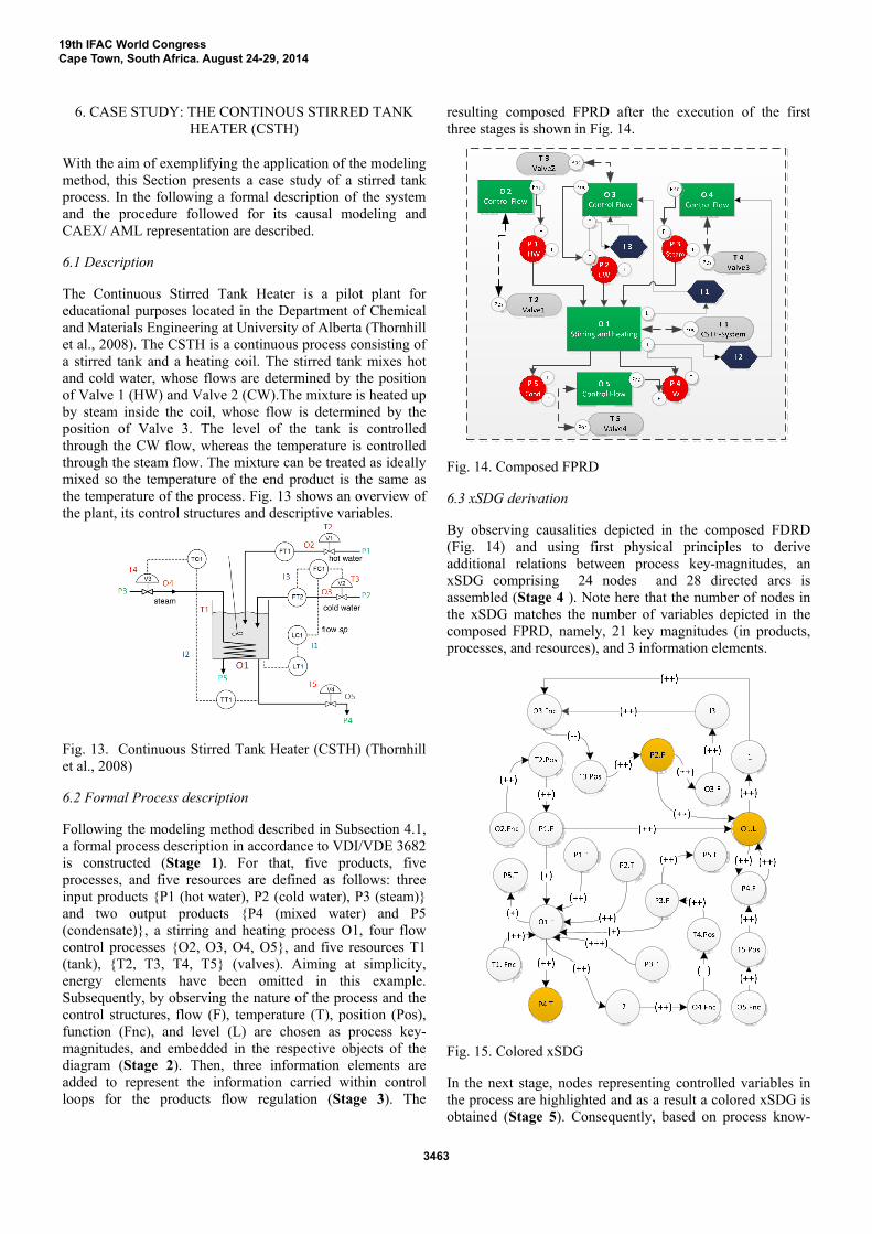
6.3 xSDG derivation

By observing causalities depicted in the composed FDRD (Fig. 14) and using first physical principles to derive additional relations between process key-magnitudes, an xSDG comprising 24 nodes and 28 directed arcs is assembled (Stage 4 ). Note here that the number of nodes in the xSDG matches the number of variables depicted in the composed FPRD, namely, 21 key magnitudes (in products, processes, and resources), and 3 information elements.

Fig. 15. Colored xSDG

In the next stage, nodes representing controlled variables in the process are highlighted and as a result a colored xSDG is obtained (Stage 5). Consequently, based on process know-

19th IFAC World CongressCape Town, South Africa. August 24-29, 2014

3463

how, expected values are assigned to the directed arcs in accordance to Table 2 (Stage 6). Then, the digraph is verified to determine if a simplification due to multiple unmeasured nodes is required (Stage 7). In this case, even though unmeasured nodes exist, a simplification is not required since there are no configurations of several unmeasured nodes in series. At this point, the definition of consistent directed arc values based on process data is carried out (Stage 8). By using a MATLAB Simulink model built and validated by one of the authors in previous research (Thornhill et al., 2008), the process is simulated both in normal operation mode and under the influence of two faults, namely an unintentional change of the position of Valve 1 (V1) and an increase of the temperature of the cold water inflow (CW). Thereby, process data is archived and subsequently used to train edge values. The training algorithm observes the states of adjacent nodes and accordingly calculates the respective value of the linking edge by using fuzzy inference, as explained in Subsection 3.3. Fig. 15 depicts the colored xSDG obtained after the execution of the first eight stages.

6.4 CAEX/AML representation

Once the colored xSDG is obtained (see Fig. 15), the last stage (Stage 9) consists in representing the model in CAEX/AML as discussed in Section 5. For that, the nine- steps procedure (Subsection 5.3) is followed and as a result an XML-based and OO oriented model is obtained. A segment of the resulting model is illustrated in Fig. 12. Due to space constraints, no additional screenshots are presented in this section, however the complete model can be found at http://aut.hsu-hh.de/dependability and http://personal-pages.ps.ic.ac.uk/~nina/CSTHSimulation/index.htm.

7. CONCLUSIONS AND FUTURE WORK

This paper has presented a new modeling approach to deriving causal models based on formalized process knowledge, xSDGs, and fuzzy logic. Additionally, the digital description of such causal models has been addressed by proposing a CAEX/AutomationML model representation which targets independence of the searching algorithm implementation, effective data access, seamless information exchange, and easy maintenance. Aiming at supporting the user at the description task, detailed modeling procedures for both the causal model derivation and its digital representation have been given.

Currently, the authors work in the causal model validation in order to refine the criteria for defining key-process magnitudes and the use of first physical principles, and assure thus modeling correctness and completeness.

Future work includes the creation of a tool allowing the automatic conversion of the colored xSDG (causal model) represented in MS Visio® into a CAEX/AutomationML representation by using the herein defined AML class libraries. This tool will be compliant with the AutomationML modeling procedure developed in this contribution.

REFERENCES

Ahn, S., Chang, L., Jung, Y., Han, et al (2008). Fault diagnosis of the multi-stage flash desalination process based on signed digraph and dynamic partial least square, Desalination, 228 (1-3), pp. 68-83.

AutomationML consortium (2010). Whitepaper AutomationML Part 2- AutomationML Libraries.

Chang, C. and Yu, C (1990). On-Line Fault Diagnosis using the Signed Direct Graph. Ind. Eng. Chem. Res, 29, pp. 1290-1299.

Chiang, L., Russell, E. and Braatz, R (2001). Fault Detection and Diagnosis in Industrial Systems. Springer.

Christiansen, L., Fay, A., Opgenoorth, B. and Neidig, J (2011). Improved diagnosis by combining structural and process knowledge. Proc. of IEEE Int. Conf. on Emerging Technologies & Factory Automation, pp.1-8.

Gao, D., Zhang, B., Ma, X. and Wu, C (2009). SDG multiple fault diagnosis by fuzzy logic and real-time bidirectional inference, Int. Conf. on Information Engineering and Computer Science, pp.1-8.

Han, C., Shih, R. and Lee, L (2004). Quantifying Signed Directed Graphs with the fuzzy set for Fault Diagnosis resolution improvement. Ind. Eng. Chem. Res, 33 (8), pp. 1943-1954.

IEC 62424: Specification for representation of process control engineering requests in P&I diagrams and data exchange between P&ID tools and PCE-CAE

Kramer, M. and Palowitch B.L (1987). A rule-based approach to Fault Diagnosis using the Signed Direct Graph. AIChE J., p.p. 233-243

Lü, N., Xiong, Z., Xiong, W. and Ren, C (2011). Integrated framework of probabilistic Signed Digraph based fault

diagnosis approach to a gas fractionation unit. Ind Eng. Chem. Res, 50 (17), pp. 10062-10073

Lüder, A., Schmidt, N. and Helgermann, S (2013). Lossless exchange of graph based structure information of production systems by AutomationML. Proc. of IEEE Int. Conf. on Emerging Technologies & Factory Automation.

Shih, R. and Lee, L (1995). Use of fuzzy cause-effect digraph for resolution fault diagnosis for process plants: fuzzy cause-effect digraph. Ind. Eng. Chem. Res. 34, pp. 1688-1702.

Thornhill, N.F, Patwardhan, S. and Shah. S (2008). A continuous stirred tank heater simulation model with applications. J. Process Control, 18, pp. 347-360.

Ulrich, A (2009). Development methodology for the design of process plants. VDI, 425, VDI Verlag, Düsseldorf.

VDI/VDE-Guideline 3682 (2005): Formalized Process Description.

Yang, F., Shah, S. and Xiao, D (2012). Signed Directed Graph based modeling and its validation from process knowledge and process data. Int. J. Applied Math and Computational Science, 22, pp. 41-53.

Zhang, J., Cao, W., Wang, B. and Cui, N (2005). Fault location algorithm based on the qualitative and quantitative knowledge of signed directed graph, Proc. of IEEE Int. Conf. on Industrial Technology, pp.1231-1234.

19th IFAC World CongressCape Town, South Africa. August 24-29, 2014

3464