Market Segmentation with Latent Class Regression

Deqiang Zou | School of Management | Fudan University

Applications of the package “FlexMix”November 14, 2010 @ Shanghai University of Finance and Economics

Segment and Segmentation• A segment is a group of end‐users that share a unique set of wants/needs and/or purchase behaviors

• Segmentation is the process that companies use to divide large heterogeneous markets into small markets that can be reached more efficiently and effectively with products and services that match their unique needs

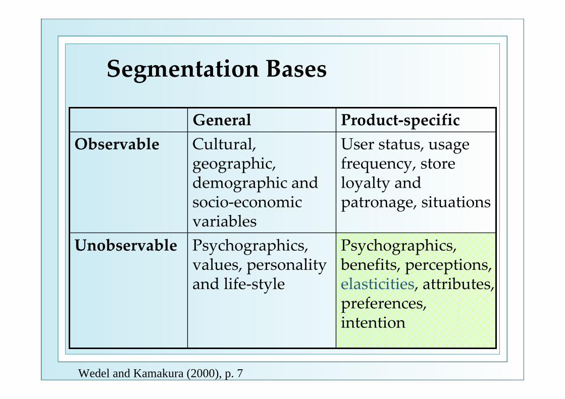
Segmentation Bases

Psychographics, benefits, perceptions, elasticities, attributes, preferences, intention

Psychographics, values, personality and life‐style

Unobservable

User status, usage frequency, store loyalty and patronage, situations

Cultural, geographic, demographic and socio‐economic variables

ObservableProduct‐specificGeneral

Wedel and Kamakura (2000), p. 7

Pricing Segments

p

q

p

q

Brand Loyals Deal Prone

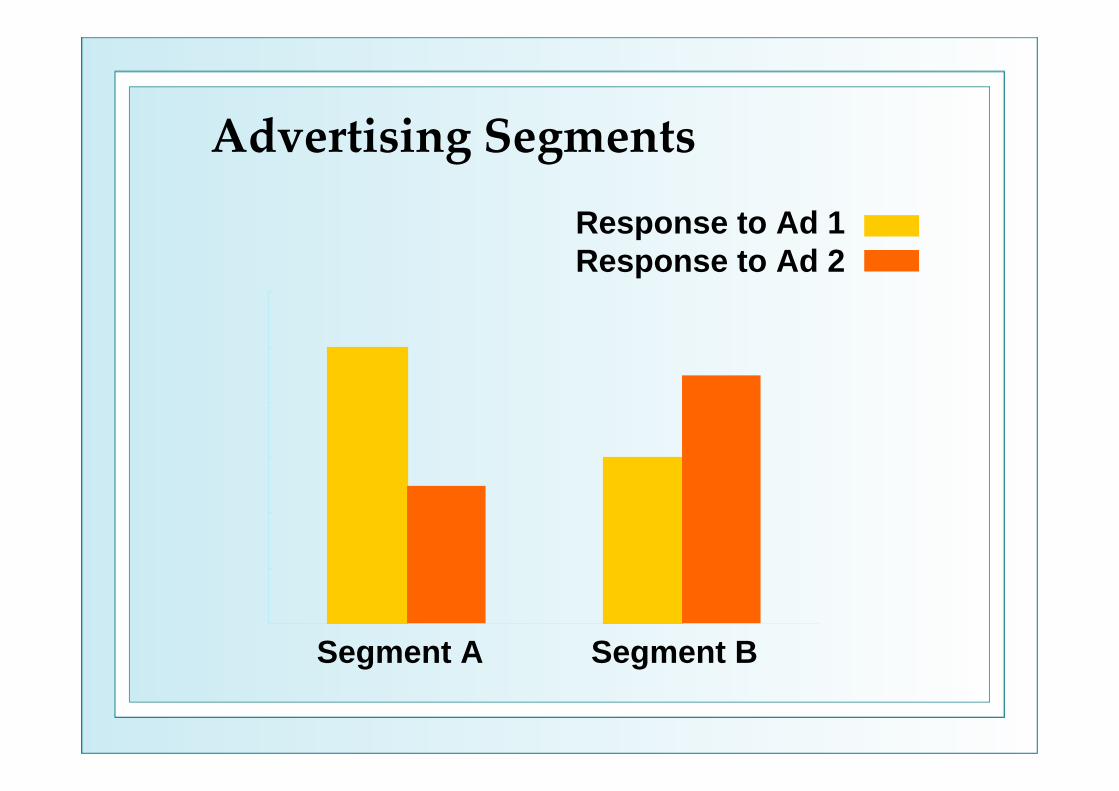
Advertising Segments

Segment A Segment B

Response to Ad 1Response to Ad 2

Segmentation Methods

AID, CART, Clusterwise regression, ANN, mixture models

Cross‐tabulation, Regression, logitand Discriminantanalysis

Predictive

Clustering methods: Nonoverlapping, overlapping, Fuzzy techniques, ANN, mixture models

Contingency tables, Log‐linear models

Descriptive

Post hoca priori

Wedel and Kamakura (2000), p. 17

Segmentation: Distance?

Segment4

Segment3

Segment2

Segment1

Segment4

Segment3

Segment2

Segment1

Low High Low HighSatisfactionEducation

Inco

me

Rep

urch

ase

Low

Hig

h

Low

Hig

h

• Segmentation is the process of clustering consumers on basis of distances between them?

Aggregate (100%): Loyal= -2.46 + 1.06×SatisfactionSegment A (25.22%): Loyal= 1.65 + 0.77×SatisfactionSegment B (48.38%): Loyal= -4.25 + 1.33×SatisfactionSegment C (26.40%): Loyal= 0.17 + 0.33×Satisfaction

Segmentation with Cause‐Effect Relation

王霞, 赵平, 王高, 刘佳 (2005)

Multiple Correspondence Analysis

Segment C•College or above•Average or high income•Age<30

Segment A•Senior high school•Modest income•40<Age<50

Segment B•Primary school or junior high school•Lowest income•Age>50

王霞, 赵平, 王高, 刘佳 (2005)

Relationship for Segment Targeting

DescriptorVariables

DescriptorVariables

BehavioralVariables

BehavioralVariables

Identifying the Particular Members of a Segment

The Aspects of a Segment that Define Marketers’

Efforts

The Key to Targeting a Segment

Latent Class Regression• Clusterwise / (finite) mixture regression

− Consider finite mixture models with K components of form

− πk≥0,

− where y is a (possibly multivariate) dependent variable with conditional density h, x is a vector of independent variables, πk is the prior probability of component k, θk is the component specific parameter vector for the density function f, and ψ= (π1, …, πK , θ’1,…, θ’K)’ is the vector of all parameters

1( | , ) ( | , )ψ π θ

=

=∑K

k kk

h y x f y x

11π

=

=∑K

kk

(1)

Latent Class Regression• If f is a univariate normal density with 

component‐specific mean β’kx and variance σk2 , we have θk = (β’k, σk2) and Equation (1) describes a mixture of standard linear regression models

• If f is a member of the exponential family, we get a mixture of generalized linear models

Posterior Probability• The posterior probability that observation (x, y) 

belongs to class j is given by

• The posterior probabilities can be used to segment data by assigning each observation to the class with maximum posterior probability

• Individual‐level predictions of finite mixture models are a weighted combination of the segment‐level regression functions, weighted with the posterior membership probabilities (DeSarbo, Kamakura, and Wedel 2006)

( | , )( | , , )

( | , )π θ

ψπ θ

=∑

i j

k kk

f y xP j x y

f y x

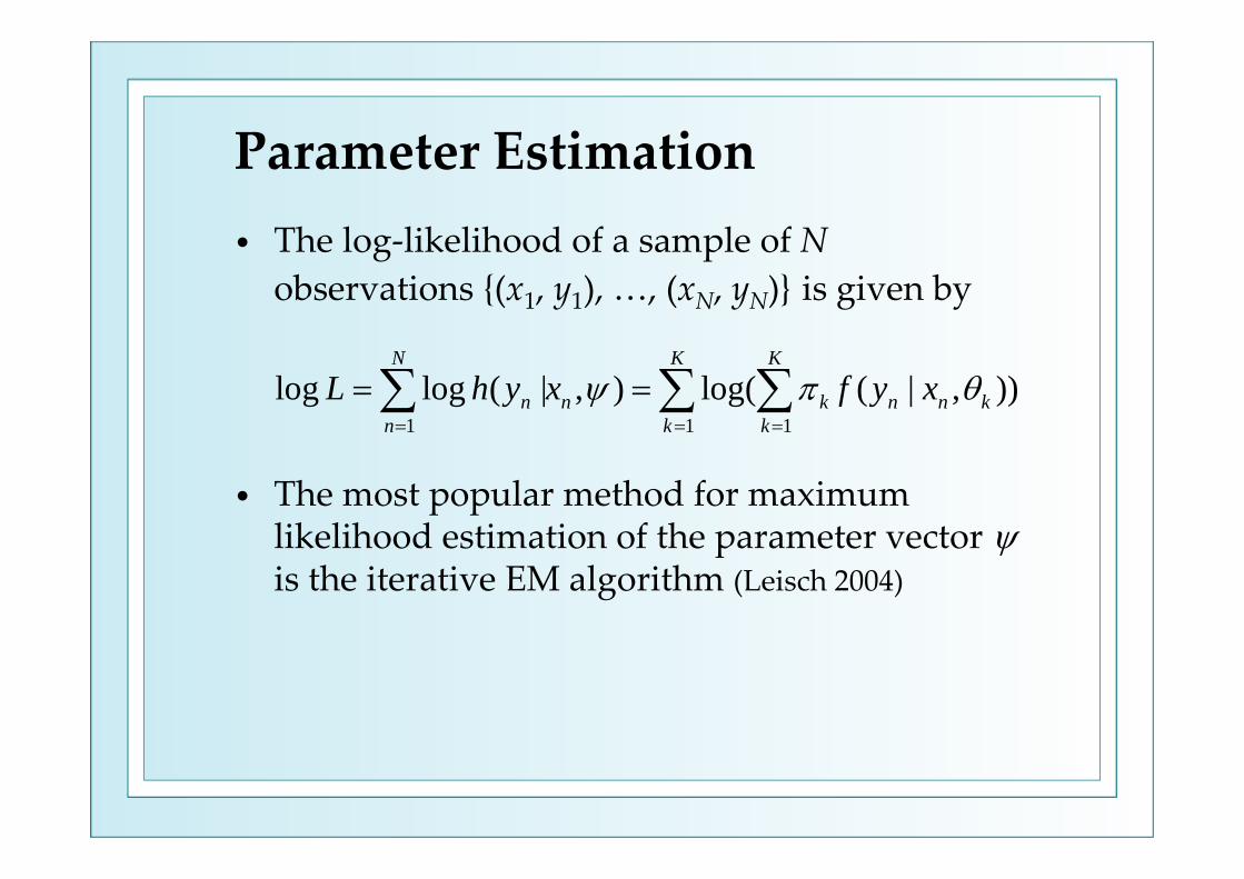
Parameter Estimation• The log‐likelihood of a sample of N

observations {(x1, y1), …, (xN, yN)} is given by

• The most popular method for maximum likelihood estimation of the parameter vector ψis the iterative EM algorithm (Leisch 2004)

1 1 1

log log ( | , ) log( ( | , ))ψ π θ= = =

= =∑ ∑ ∑N K K

n n k n n kn k k

L h y x f y x

Using FlexMix• As a simple example we use artificial data with 

two latent classes of size 100 each:− Class 1: y = 5x + ε− Class 2: y = 15 + 10x − x2 + ε

− with ε~ N(0, 9) and prior class probabilities π 1 = π 2 = 0.5

• We can fit this model in R using the commands

Leisch (2004)

> library(flexmix)> data(NPreg)> m1 = flexmix(yn ~ x + I(x^2), data = NPreg, k = 2)> m1

Leisch (2004)

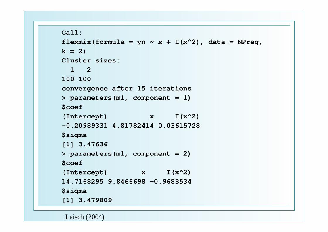
Call:flexmix(formula = yn ~ x + I(x^2), data = NPreg,k = 2)Cluster sizes:1 2

100 100convergence after 15 iterations> parameters(m1, component = 1)$coef(Intercept) x I(x^2)-0.20989331 4.81782414 0.03615728$sigma[1] 3.47636> parameters(m1, component = 2)$coef(Intercept) x I(x^2)14.7168295 9.8466698 -0.9683534$sigma[1] 3.479809

Leisch (2004)

Using FlexMix> summary(m1)Call:flexmix(formula = yn ~ x + I(x^2), data = NPreg,k = 2)

prior size post>0 ratioComp.1 0.494 100 145 0.690Comp.2 0.506 100 141 0.709`log Lik.' -642.5453 (df=9)AIC: 1303.091 BIC: 1332.775> table(NPreg$class, m1@cluster)

1 21 95 52 5 95

Leisch (2004)

Significance Test

Leisch (2004)

> rm1 = refit(m1)> summary(rm1)Call:refit(m1)Component 1 :

Estimate Std. Error t value Pr(>|t|)(Intercept) -0.208996 0.673900 -0.3101 0.7568x 4.817015 0.327447 14.7108 <2e-16I(x^2) 0.036233 0.032545 1.1133 0.2669-------------Component 2 :

Estimate Std. Error t value Pr(>|t|)(Intercept) 14.717541 0.890843 16.521 < 2.2e-16x 9.846148 0.390385 25.222 < 2.2e-16I(x^2) -0.968304 0.036951 -26.205 < 2.2e-16

Automated Model Search• In real applications the number of components 

is unknown and has to be estimated• Fit models with an increasing number of 

components and compare them using AIC or BIC

• Choose the number of components minimizing the BIC

Leisch (2004)

> m7 = stepFlexmix(yp ~ x + I(x^2), data = NPreg, control = list(verbose = 0), K = 1:5, nrep = 5)> sapply(m7, BIC)

1 2 3 4 5946.7477 925.9972 942.1553 960.0626 960.9347

Finite Mixtures with Concomitant Variables• If the weights depend on further variables, 

these are referred to as concomitant variables• The model class is given by

− Where w denotes the concomitant variables, α are the parameters of the concomitant variable model

Grün and Leisch (2008)

1( | , , ) ( , ) ( | , )

K

k k kk

h y x f y xω ψ π ω α θ=

=∑

1

( , ) 1K

kk

π ω α=

=∑ ( , ) 0,k kπ ω α > ∀

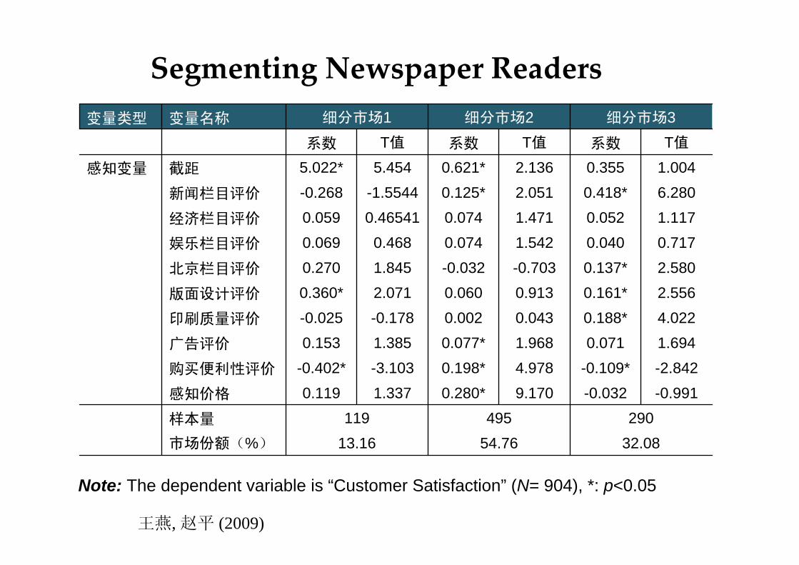
32.0854.7613.16市场份额（%）

290495119样本量

-0.991-0.0329.1700.280*1.3370.119感知价格

-2.842-0.109*4.9780.198*-3.103-0.402*购买便利性评价

1.6940.0711.9680.077*1.3850.153广告评价

4.0220.188*0.0430.002-0.178-0.025印刷质量评价

2.5560.161*0.9130.0602.0710.360*版面设计评价

2.5800.137*-0.703-0.0321.8450.270北京栏目评价

0.7170.0401.5420.0740.4680.069娱乐栏目评价

1.1170.0521.4710.0740.465410.059经济栏目评价

6.2800.418*2.0510.125*-1.5544-0.268新闻栏目评价

1.0040.3552.1360.621*5.4545.022*截距感知变量

T值系数T值系数T值系数

细分市场3细分市场2细分市场1变量名称变量类型

Segmenting Newspaper Readers

Note: The dependent variable is “Customer Satisfaction” (N= 904), *: p<0.05

王燕, 赵平 (2009)

1.1850.9481.0360.7254000元以上

-1.291-0.746-3.055-1.689*2000-4000元家庭月收入g

0.8990.542-0.344-0.23525-35岁-1.228-0.7720.2920.16325岁以下

年龄f

2.6381.319*2.0911.016*高中及以下

教育程度e

1.4140.6432.7961.138*男

性别d

-0.002-0.0010.1930.125上班

-1.451-0.9660.7050.492家中

阅读地点c

2.6581.327*1.5720.644半小时以下

每次读报用时b

0.3780.188-0.162-0.069每天阅读

阅读频率a

-0.503-0.5780.0750.081截距个人特征变量

T值系数T值系数T值系数

细分市场3细分市场2细分市场1变量名称变量类型

Recap• The underlying basis of customer 

heterogeneity (i.e., discrete market segments) is unknown a priori

• The objective is to simultaneously estimate the number of market segments, their size and composition, and the segment specific regression coefficients

• Concomitant variable mixtures allow for demographic variables to explain segment membership simultaneously

• This class of methods enables marketers to engage in response‐based segmentation, i.e., from descriptive to predictive segmentation

References (I)• 王霞, 赵平, 王高, 刘佳 (2005), “基于顾客满意和顾客忠诚

关系的市场细分方法研究,”南开管理评论, 8 (5), 26‐30.• 王燕, 赵平 (2009), “伴生变量混合模型在市场细分中的应

用,”营销科学学报, 5 (1), 27‐34. (http://www.jms.org.cn/read/15/3.pdf)

• Grün, Bettina and Friedrich Leisch (2008), “FlexMixVersion 2: Finite Mixtures with Concomitant Variables and Varying and Constant Parameters,” Journal of Statistical Software, 28 (4), (http://www.jstatsoft.org/v28/i04)

• Leisch, Friedrich (2004), “FlexMix: A General Framework for Finite Mixture Models and Latent Class Regression in R,” Journal of Statistical Software, 11 (8), (http://www.jstatsoft.org/v11/i08)

References (II)• Desarbo, Wayne S., Wagner A. Kamakura, and Michel 

Wedel (2006), “Latent Structure Regression,” in Rajiv Grover and Marco Vriens (Eds.), The Handbook of Marketing Research: Uses, Misuses, and Future Advances, Thousand Oaks: Sage Publications.

• McLachlan, Geoffrey and David Peel (2000), Finite Mixture Models, Now York: John Wiley & Sons, Inc.

• Wedel, Michel and Wagner A. Kamakura (2001), Market Segmentation: Conceptual and Methodological Foundations (2nd Edition), Boston: Kluwer Academic Publishers.

Q & A• Your comments are appreciated