Embed Size (px)
Citation preview

Depth-averaged Models and Softwarefor Geophysical Flows
Randall J. LeVequeDepartment of Applied Mathematics
University of Washington
GeoClaw: http://www.clawpack.org
R. J. LeVeque SIAM Annual Meeting, July 9, 2008

Collaborators
David George, University of WashingtonSoon to be Mendenhall postdoctoral Fellow at theUSGS Cascades Volcano Observatory (CVO)
Marsha Berger, Courant Institute, NYU
Roger Denlinger and Dick Iverson,USGS Cascades Volcano Observatory (CVO)
David Alexander and William Johnstone,Spatial Vision Group, Vancouver, BC
Barbara Lence, Civil Engineering, UBC
Harry Yeh, Civil Engineering, OSU
Numerous other students and colleagues
Supported in part by NSF
R. J. LeVeque SIAM Annual Meeting, July 9, 2008

Outline
• Why use depth-averaged models?• Current and potential applications• Why AMR is often crucial
• Shallow water equations• Dry states and margins• Steady states and well-balancing
• Depth-averaged models of complex flows• Other applications• Some mathematical challenges
R. J. LeVeque SIAM Annual Meeting, July 9, 2008
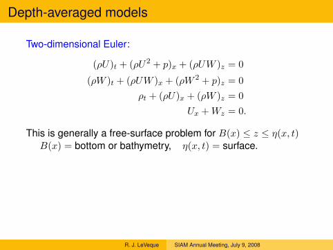
Depth-averaged models
Two-dimensional Euler:
(ρU)t + (ρU2 + p)x + (ρUW )z = 0
(ρW )t + (ρUW )x + (ρW 2 + p)z = 0ρt + (ρU)x + (ρW )z = 0
Ux + Wz = 0.
This is generally a free-surface problem for B(x) ≤ z ≤ η(x, t)B(x) = bottom or bathymetry, η(x, t) = surface.
Assume:
ρ(x, z, t) = constant (homogeneous density)W (x, z, t) = 0 (vertical velocity negligible)p(x, z, t) = g(η(x, t)− z) (hydrostatic pressure)
R. J. LeVeque SIAM Annual Meeting, July 9, 2008

Depth-averaged models
Let
h(x, t) = η(x, t)−B(x), (fluid depth)
u(x, t) =1
h(x, t)
∫ η(x,t)
B(x)U(x, z, t) dz.
Integrate Euler equations in z to obtain p = 12gh2 and ...
One-dimensional Shallow Water (St. Venant) Equations
ht + (hu)x = 0
(hu)t +(hu2 +
12gh2
)x
= −ghB′(x)
R. J. LeVeque SIAM Annual Meeting, July 9, 2008

Depth-averaged models
Similary, reduce three-dimensional free surface problem to...
Two-dimensional Shallow Water (St. Venant) Equations
ht + (hu)x + (hv)y = 0
(hu)t +(hu2 +
12gh2
)x
+ (huv)y = −ghBx(x, y)
(hv)t + (huv)x +(hv2 +
12gh2
)y
= −ghBy(x, y)
where (u, v) are velocities in the horizontal directions (x, y).
R. J. LeVeque SIAM Annual Meeting, July 9, 2008

Depth-averaged models
Advantages:• 2D rather than 3D
Often critical for realistic geophysical flowsVastly different spatial scales, e.g. ocean to harborNeed Adaptive Mesh Refinement even in 2D!
• No free surface η(x, y, t).
Possible problems:• When is this valid?• What if fluid is not homogeneous, or
shallow water assumptions don’t hold?• Often still a free boundary in te x-y domain,
at the shoreline or at the margins of the flow.• Small perturbations to steady state hard to capture.
R. J. LeVeque SIAM Annual Meeting, July 9, 2008

Tsunamis
Generated by• Earthquakes,• Landslides,• Submarine landslides,• Volcanoes,• Meteorite or asteroid impact
There were 97 significant tsunamis during the 1990’s,causing 16,000 casualties.
There have been approximately 28 tsunamis with run-upgreater than 1m on the west coast of the U.S. since 1812.
R. J. LeVeque SIAM Annual Meeting, July 9, 2008

Tsunamis
• Small amplitude in ocean (< 1 meter) but can grow to10s of meters at shore.
• Run-up along shore can inundate 100s of meters inland
• Long wavelength (as much as 200 km)
• Propagation speed√
gh (much slower near shore)
• Average depth of Pacific or Indian Ocean is 4000 m=⇒ average speed 200 m/s ≈ 450 mph
R. J. LeVeque SIAM Annual Meeting, July 9, 2008

Sumatra event of December 26, 2004Magnitude 9.1 quake near Sumatra, where Indian tectonic plateis being subducted under the Burma platelet.
Rupture along subduction zone≈ 1200 km long, 150 km wide
Propagating at ≈ 2 km/sec (for ≈ 10 minutes)
Fault slip up to 15 m, uplift of several meters.(Fault model from Caltech Seismolab.)
www.livescience.com
R. J. LeVeque SIAM Annual Meeting, July 9, 2008
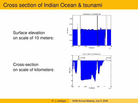
Cross section of Indian Ocean & tsunami
Surface elevationon scale of 10 meters:
Cross-sectionon scale of kilometers:
R. J. LeVeque SIAM Annual Meeting, July 9, 2008

Shallow water equations with bathymetry B(x, y)
ht + (hu)x + (hv)y = 0
(hu)t +(
hu2 +12gh2
)x
+ (huv)y = −ghBx(x, y)
(hv)t + (huv)x +(
hv2 +12gh2
)y
= −ghBy(x, y)
Some issues:
• Delicate balance between flux divergence and bathymetry:h varies on order of 4000m, rapid variations in oceanWaves have magnitude 1m or less.
• Cartesian grid used, with h = 0 in dry cells:Cells become wet/dry as wave advances on shoreRobust Riemann solvers needed.
• Adaptive mesh refinement crucialInteraction of AMR with source terms, dry states
R. J. LeVeque SIAM Annual Meeting, July 9, 2008

Tsunami simulations
• 2D shallow water + bathymetry
• Finite volume method• Cartesian grid
• Cells can be dry (h = 0)
• Cells become wet/dry as wavemoves on shore
• Mesh refinement on rectangularpatches
• Adaptive — follows wave, morelevels near shore
R. J. LeVeque SIAM Annual Meeting, July 9, 2008

Local modeling near Chennai (Madras), India
R. J. LeVeque SIAM Annual Meeting, July 9, 2008
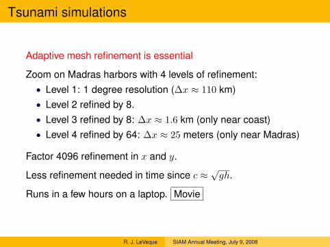
Tsunami simulations
Adaptive mesh refinement is essential
Zoom on Madras harbors with 4 levels of refinement:• Level 1: 1 degree resolution (∆x ≈ 110 km)• Level 2 refined by 8.• Level 3 refined by 8: ∆x ≈ 1.6 km (only near coast)• Level 4 refined by 64: ∆x ≈ 25 meters (only near Madras)
Factor 4096 refinement in x and y.
Less refinement needed in time since c ≈√
gh.
Runs in a few hours on a laptop. Movie
R. J. LeVeque SIAM Annual Meeting, July 9, 2008

Cascadia subduction fault
• 1200 km long off-shore fault stretching from northern California tosouthern Canada.
• Last major rupture: magnitude 9.0 earthquake on January 26, 1700.
• Tsunami recorded in Japan with run-up of up to 5 meters.
• Historically there appear to be magnitude 8 or larger quakes every 500years on average.
R. J. LeVeque SIAM Annual Meeting, July 9, 2008
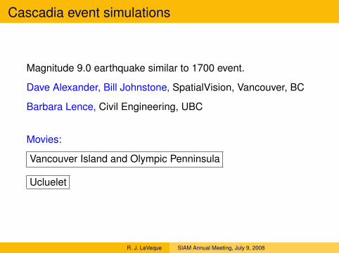
Cascadia event simulations
Magnitude 9.0 earthquake similar to 1700 event.
Dave Alexander, Bill Johnstone, SpatialVision, Vancouver, BC
Barbara Lence, Civil Engineering, UBC
Movies:
Vancouver Island and Olympic Penninsula
Ucluelet
R. J. LeVeque SIAM Annual Meeting, July 9, 2008

Hazard Study for Tofino, BC
R. J. LeVeque SIAM Annual Meeting, July 9, 2008

Hazard Study for Tofino, BC
R. J. LeVeque SIAM Annual Meeting, July 9, 2008

Hazard Study for Tofino, BC
R. J. LeVeque SIAM Annual Meeting, July 9, 2008

Hazard Study for Tofino, BC
R. J. LeVeque SIAM Annual Meeting, July 9, 2008

Comparison to NOAA model
Thanks to Tim Walsh (WA State DNR)
R. J. LeVeque SIAM Annual Meeting, July 9, 2008

GeoClaw Software
TsunamiClaw: Dave George’s code based on Clawpack.
Recently made more general as GeoClaw.
Currently includes:• 2d library for depth-averaged flows over topography.• Well-balanced Riemann solvers that handle dry cells.• General tools for dealing with multiple data sets at different
resolutions.• Tools for specifying regions where refinement is desired.• Graphics routines (Matlab currently, moving to Python).• Output of time series at gauge locations or on fixed grids.
R. J. LeVeque SIAM Annual Meeting, July 9, 2008
GeoClaw
Future:• Other depth-averaged flow rheologies• Two-dimensional vertical slices,
full 3D models for flow on topography• Subsurface flows, seismology, etc.
Test version recently released as part of Clawpack 5.0see www.clawpack.org.
Some other new features:• Python interface tools and open source graphics• EagleClaw (Easy Access Graphical Laboratory for
Exploring Conservation Laws)
• Will include other generalizations such as DavidKetcheson’s WENOCLAW (high order methods).
R. J. LeVeque SIAM Annual Meeting, July 9, 2008

Some other applications
Shallow water equations:• Storm surges, hurricanes• River flooding• Dam breaks
More complex flows:• Flow on steep terrain• Debris flows and lahars• Lava flows• Pyroclastic flows and surges• Landslides and avalanches• Underwater landslides / tsunami generation• Multi-layer, internal waves
R. J. LeVeque SIAM Annual Meeting, July 9, 2008

Debris flows
movie
R. J. LeVeque SIAM Annual Meeting, July 9, 2008
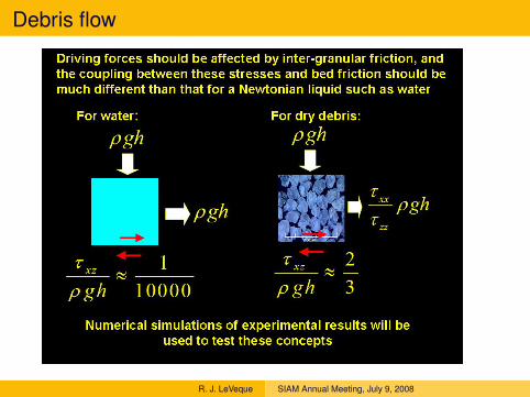
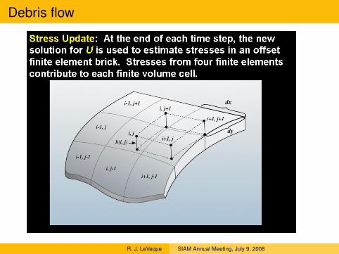
Debris flow
R. J. LeVeque SIAM Annual Meeting, July 9, 2008
Debris flow
R. J. LeVeque SIAM Annual Meeting, July 9, 2008

Debris flow
R. J. LeVeque SIAM Annual Meeting, July 9, 2008

Table top sand flume
R. J. LeVeque SIAM Annual Meeting, July 9, 2008

Table top sand flume
R. J. LeVeque SIAM Annual Meeting, July 9, 2008

Flume
initiation runout
R. J. LeVeque SIAM Annual Meeting, July 9, 2008

Challenges for applied mathematicians
Mathematical modeling and analysis:• Proper models for depth averaging complex rheologies• Understanding mathematical structure, e.g.
– Well posedness of equations– Loss of hyperbolicity in multi-layer equations– Proper interpretation of products of distributions
Algorithm development:• Robust methods for dry states, well-balancing• AMR error estimation, adjoint methods?• Nonlinear nonconservative products
R. J. LeVeque SIAM Annual Meeting, July 9, 2008

Challenges for applied mathematicians
Working with real topography/bathymetry data:• Interpolation of scattered nonsmooth noisy data• Automatic smoothing of mismatches between topo/bathy
Some challenging applications:• Erosion and sedimentation,
tsunami deposits, geomorphology• Debris flows, land slides, avalanches• Lava flows• Many more — American Geophysical Union annual
meeting is a good source of problems!
Collaborate with earth scientists for maximal impact.
R. J. LeVeque SIAM Annual Meeting, July 9, 2008