Embed Size (px)
Citation preview

Compositional closurefor Bayes Risk
in probabilistic noninterference
Annabelle McIver1, Larissa Meinicke1, and Carroll Morgan2?
1 Dept. Computer Science, Macquarie University, NSW 2109 Australia2 School of Comp. Sci. and Eng., Univ. New South Wales, NSW 2052 Australia
Abstract. We give a sequential model for noninterference security in-cluding probability (but not demonic choice), thus supporting reasoningabout the likelihood that high-security values might be revealed by obser-vations of low-security activity. Our novel methodological contribution isthe definition of a refinement order (v) and its use to compare securitymeasures between specifications and (their supposed) implementations.This contrasts with the more common practice of evaluating the securityof individual programs in isolation.
The appropriateness of our model and order is supported by our show-ing that (v) is the greatest compositional relation –the compositionalclosure– with respect to our semantics and an “elementary” order basedon Bayes Risk — a security measure already in widespread use. We alsorelate refinement to other measures such as Shannon Entropy.
By applying the approach to a non-trivial example, the anonymous-majority Three-Judges protocol, we demonstrate by example that cor-rectness arguments can be simplified by the sort of layered developments–through levels of increasing detail– that are allowed and encouraged bycompositional semantics.
? We acknowledge the support of the Australian Research Council Grant DP0879529.
arX
iv:1
007.
1054
v1 [
cs.F
L]
7 J
ul 2
010

Table of Contents
Compositional closure for Bayes Risk in probabilistic noninterference . . . . 1Annabelle McIver, Larissa Meinicke, Carroll Morgan1 Introduction . . . . . . . . . . . . . . . . . . . . . . . . . . . . . . . . . . . . . . . . . . . . . . . . . . . 32 A probabilistic, noninterference sequential semantics . . . . . . . . . . . . . . . . 73 The Bayes-Risk based elementary testing order . . . . . . . . . . . . . . . . . . . . 134 Non-compositionality of the elementary testing order . . . . . . . . . . . . . . . 145 The refinement order, and compositional closure . . . . . . . . . . . . . . . . . . . 146 Constructive definition of the refinement order . . . . . . . . . . . . . . . . . . . . . 157 Refinement (v) is the compositional closure of (�) . . . . . . . . . . . . . . . . . 188 Case study: The Three Judges protocol . . . . . . . . . . . . . . . . . . . . . . . . . . . 249 Conclusion: a challenge and an open problem . . . . . . . . . . . . . . . . . . . . . . 37A Proofs for partition-based matrix representations . . . . . . . . . . . . . . . . . . . 44B Secure semantics via matrices . . . . . . . . . . . . . . . . . . . . . . . . . . . . . . . . . . . 44C Proofs for the refinement relation . . . . . . . . . . . . . . . . . . . . . . . . . . . . . . . . 49D Example of completeness construction . . . . . . . . . . . . . . . . . . . . . . . . . . . . 52E Proof of the Atomicity Lemma . . . . . . . . . . . . . . . . . . . . . . . . . . . . . . . . . . 55F Informal description of the Oblivious Transfer implementation 3 . . . . . . 57G Alternative uncertainty measures . . . . . . . . . . . . . . . . . . . . . . . . . . . . . . . . 58

Compositional closure for Bayes Risk in probabilistic noninterference 3
1 Introduction
We apply notions of testing equivalence and refinement, based on Bayes Risk, tothe topic of noninterference security [10] with probability but without demonicchoice. Previously, we have studied noninterference for demonic systems withoutprobabilistic choice [26, 27], and we have studied probability and demonic choicewithout noninterfence [28, 21]. Here thus we are completing a programme oftreating these features “pairwise.”
Our long-term aim –as we explain in the conclusion– is to treat all threefeatures together, based on the lessons we have learned by treating strict subsetsof them. The benefit (should we succeed) would apply not only to security,but also to conventional program development where, in the presence of bothprobabilistic and demonic choice, the technique of data-transformation (aka.data refinement or data reification) becomes unexpectedly complex: variablesinside local scopes must be treated analogously to “high security” variables innoninterference security.
We take the view, learned from others, that program/system developmentbenefits from a comparison of specification programs with (putative) implemen-tations of them, wherever this is possible, via a mathematically defined “refine-ment” relation whose formulation depends ultimately on a notion of testing thatis agreed-to subjectively by all parties concerned [8]. 4 To explain our positionunambiguously, we begin by recalling the well known effects of this approach forconventional, sequential programming.
1.1 Elementary testing and refinement for conventional programs
Consider sequential programs operating over a state-space of named variableswith fixed types, including a program abort that diverges (such as an infiniteloop). We allow demonic nondeterminsm, statements such as x:= 0 u x:= 1, inthe now-conventional way in which they represent equally abstraction (we donot care whether x is assigned 0 or 1, as long as it is one or the other), on theone hand, or unpredictable and arbitrary run-time choice on the other.
Having determined a “specification” program S, we address the question ofwhether we are prepared to accept some program I that purports to “implement”it. Although there is nowadays a widely accepted answer to this, we imagine thatwe are considering the question for the first time and that we are hoping to findan answer that everybody will accept. For that we search for a test on programsthat is “elementary” in the sense that it is conceptually simple and that no“reasonable” person could ever argue that S is implemented by I if it is the casethat S always passes the test but I might fail it. 5
4 We say “wherever this is possible” since there are many aspects of system develop-ment that cannot be pinned down mathematically. But –we argue– those that canbe, should be.
5 There is a possibly dichotomy here between “may testing” and “must testing,” andwe are taking the latter in this example: if S must pass a certain test, then so mustI if it is to be considered an implementation.

4 Annabelle McIver, Larissa Meinicke, and Carroll Morgan
A common choice for such an elementary test is “can diverge,” where diver-gence is considered to be a bad thing: using it, our criterion becomes “if I indeedimplements S and I can diverge, then it must be possible for S to diverge also.”We note that the elementary test cannot be objectively justified: it is an “ax-iom” of the approach that will be built on it; and it is via the subjective axioms(in any approach) that we touch reality, where we avoid an infinite definitionalregress.
The elementary test provides an “only if” answer to the implementationquestion, but not an “if.” That is, we do not say that I implements S if eitherI never fails the test or S might fail it: this is not practical, because of context.For an example, let S be if x 6=0 then abort fi and let I be simply abort.Then indeed S passes the test if I does (because they both fail); but we cannotaccept I generally as a replacement for S because context x:= 0;S “protects” S,and passes the test as a whole; but the same context does not protect I, sincex:= 0; I (still) fails. This illustrates the inutility of the elementary view taken onits own, and it shows that we need a more sophisticated comparison in order tohave a practical tool that respects contexts. (Thus it is clear above that we mustadd “if executed from the same initial state.”) The story leads on from hereto a definition, ultimately, of sequential-program refinement (v) as the uniquerelation such that 6
(i) soundness If SvI then for all contexts C we have that C(I) passes theelementary test if C(S) does, and
(ii) completeness If S 6vI then there is some context C such that C(I) fails theelementary test although C(S) passes it.
That relation turns out to have the direct definition that SvI just when, for allinitial states s, if executing I from s can deliver some final state s′ then –froms again– either S can deliver s′, as well, or S can diverge. Crucially, it is thedirect definition that allows (v) to be determined without examining all possiblecontexts.
1.2 Elementary testing and refinement for probabilisticnoninterference-secure programs
In attempting to follow the trajectory of §1.1 into the modern context of nonin-terference and probability, we immediately run into the problem that there arecompeting notions of elementary test. Here are just four of them:
Bayes Risk [34, 5, 1, 2] is based on the probability an attacker can reveal ahigh-security, “hidden” variable h using a single query “Is h equal to h?”where h is some value in h’s type. Here (and below) the elementary testingof S wrt. I requires that the probability of revealing h in I cannot be higherthan it is in S.
6 We say “a” rather thean “the” definition of refinement because this is just an ex-ample: other elementary tests, and other possible contexts, lead naturally to otherdefinitions.
Compositional closure for Bayes Risk in probabilistic noninterference 5
marginal guesswork [30, 15] is measured in terms of how many queries of theform “Is h equal to h?” are needed to determine h’s value with a givenprobability.
Shannon Entropy [33] is related to the use of multiple queries of the form “Ish in some set H?” where H is a subset of h’s type.
guessing entropy [19, 15] is the average number of “Is h equal to h?” guessesnecessary to determine h’s value.
Not only do these criteria compete for popularity, it turns out that on theirown they are not even objectively comparable. For instance, Pliam [30] findsthat there can be no general ordering between marginal guesswork and ShannonEntropy: that is, from a marginal-guesswork judgement of whether S passes alltests that I does, there is no way to determine whether the same would holdfor Shannon-entropy judgements, nor vice versa. Similarly, Smith has comparedBayes Risk and Shannon Entropy, and claims that these measures are inconsis-tent in the same sense [34]. The general view seems to be that none of these(four) methods can be said to be generally more- or less discriminating than anyof the others.
In spite of the above, one of our contributions here is to show that Bayes Riskis maximally discriminating among those four if context is taken into account.
1.3 Features of our approach: a summary
Our most significant deviation from traditional noninterference is that, ratherthan calculating security measures of programs in isolation, instead we focus oncomparing security measures between programs: typically one is supposed to bea specification, and another is supposed to be an implementation of it. What weare looking for is an implementation that is at least as secure as its specification.
Since we never consider the security of programs in isolation, an advantage isthat it is possible easily to arrange certain kinds of permissible information flow.For example whenever s≥i holds, a program I that leaks only the i low-orderbits of a hidden integer h is secure with respect to a specification S that leaksthe s low-order bits of h — that is, for any implementation of S, the leaking ofup to s low-order bits of h is allowed but no more. This way we sometimes canavoid separate tools for declassification: to allow an implementation to release(partial) information, we simply arrange that its specification does so.
Typically it is both functional- and security properties (however we measurethem) that are of interest. As such, we would like to define a relation (v) betweenthese programs so that SvI just when implementation I has all the functionaland the security properties that specification S does, where “all” is interpretedwithin our terms of reference. For incremental, compositional reasoning with suchan order, it has been known from the very beginning [37] that the refinementrelation (v) must satisfy two key technical properties:
Transitivity If SvMvI then also SvI. Because of this a comparison betweentwo large programs S, I can be carried out via S v M1 v · · · v MN v Ithrough many small steps over a long time.

6 Annabelle McIver, Larissa Meinicke, and Carroll Morgan
Monotonicity of contexts If S v I then also C(S) v C(I), where C is anyprogram context. Because of this, a large comparison can be carried out viamany small steps independently by a large programming team working inparallel.
As argued above, since our comparisons rest ultimately on subjective criteriafor failure, we reduce that dependency on what is essentially an arbitrary choiceby making those criteria as elementary as possible: when can you be absolutelysure that S 6vI, that refinement should fail? For this purpose we identify anelementary testing relation (�) based on Bayes Risk, such that if S 6�I then I“certainly” (but still subjectively) does not satisfy the specification S in termsof “reasonable” functional- and probabilistically secure properties.
Because our (�) is not respected by all contexts (there exist programs S, Iand context C such that S�I, yet C(S)6�C(I) in spite of that) our relation (v) ischosen so that it is smaller –i.e. more restrictive– than (�), so that it excludesjust those “apparent” refinements that can be voided by context.
Our refinement relation is the compositional closure of (�), the largest rela-tion (v) such that SvI implies C(S)�C(I) for all possible contexts C. Abusingterminology slightly, we will for simplicity say that (v) is compositional justwhen it is respected by all possible contexts C (whereas strictly speaking weshould say that all such C’s are (v)-monotonic). Further, we note that if we de-fine equivalence A∼B to be “bi-refinement” AvB and BvA then monotonicityof (v) implies that (∼) is is a congruence for all contexts C.
There are two further, smaller idiosyncracies of our approach. The first isthat we allow the high-security, “hidden” variables to be assigned-to by the pro-gram, so that it is the secrecy of the final value h′ of h that is of concern tous, not the initial value h. This is because we could not otherwise meaningfullycompare functional properties, nor would we be able to treat (sequential) com-positional contexts. The other difference, more a position we take, is that weallow an attacker both perfect recall and an awareness of implicit flow : that theintermediate values of low-security “visible” program variables are observable,even if subsequently overwritten; and that the control-flow of non-atomic pro-gram statements is observable. As shown in our case study (§8.3) it is this whichallows us to model distributed applications: there, the values of intermediatevariables can be observed (and recalled) if they are sent on an insecure channel,and the control flow of a program may be witnessed (for example) by observingwhich request an agent is instructed to fulfill.
In summary, our technical contribution is that we (i) give a sequentialsemantics for probabilistic noninterference, (ii) define the above order (�) basedon Bayes Risk, (iii) show it is not compositional, (iv) identify a compositionalsubset of it, a refinement order (v) such that SvI implies C(S)�C(I) for allcontexts C and (v) show that (v) is in fact the compositional closure of (�), sothat in fact we have S 6vI only when C(S)6�C(I) for some C.
Finally, we note (vi) that (v) is sound for the other three, competing no-tions of elementary test and that therefore Bayes-Risk testing, with context, ismaximally discriminating among them.

Compositional closure for Bayes Risk in probabilistic noninterference 7
These technical contributions further our general goal of structuring secureprotocols hierarchically and then designing/verifying them in separate pieces,a claim that we illustrate by showing how our model and our secure-programordering may be used to give an incremental development of The Three Judges,an “anonymous majority” protocol we constructed precisely to make this point.
2 A probabilistic, noninterference sequential semantics
We identify visible variables (low-security), typically v in some finite type V, andhidden variables (high-security), typically h in finite H. Variables are in sans serifto distinguish them from (decorated) values v:V, h:H they might contain. 7
As an example, let hidden h: {0, 1, 2} represent one of three boxes: Box 0has two black balls; Box 1 has one black- and one white ball; and Box 2 hastwo white balls. Then let v: {w, b,⊥} represent a ball colour: white, black orunknown. Our first experiment in this system is Program S, informally writtenh:= 0⊕1⊕2; v:∈{{w@ h
2 , b@1− h2 }}; v:=⊥, that chooses box h uniformly, and then
draws a ball v from that Box h: from the description above (and the code) wecan see that with probability h/2 the ball is white, and with probability 1−h/2it is black. Then the ball is replaced. A typical security concern is “How muchinformation about h is revealed by its assignments to v?”
We use this program, and that question, to motivate our program syntax andsemantics, to make Program S the above program precise and to provide theframework for asking –and answering– such security questions.
We begin by introducing distribution notation, generalising the notations fornaıve set theory.
2.1 Distributions: explicit, implicit and expected values over them
We write function application as f.x, with “.” associating to the left. Operatorswithout their operands are written between parentheses, as (�) for example.Set comprehensions are written as {s:S | G · E} meaning the set formed byinstantiating bound variable s in the expression E over those elements of Ssatisfying formula G. 8
By DS we mean the set of discrete sub-distributions on set S that sum to nomore than one, and DS means the full distributions that sum to one exactly. Thesupport dδe of (sub-)distribution δ:DS is those elements s in S with δ.s 6=0, andthe weight
∑δ of a distribution is (
∑s: dδe · δ.s) , so that full distributions have
7 We say hidden and visible, rather than high- and low security, because of the con-nection with data refinement where the same technical issues occur but there are nosecurity implications.
8 This is a different order from the usual notation {E | s∈S∧G}, but we have good rea-sons for using it: calculations involving both sets and quantifications are made morereliable by a careful treatment of bound variables and by arranging that the orderS/G/E is the same in both comprehensions and quantifications (as in (∀s:S | G · E )and (∃s:S | G · E )).

8 Annabelle McIver, Larissa Meinicke, and Carroll Morgan
weight 1. Distributions can be scaled and summed according to the usual point-wise extension of arithmetic to real-valued functions, so that (c∗δ).s is c∗(δ.s)for example; the normalisation of a (sub-)distribution δ is defined [δ]:= δ/
∑δ.
Here are our notations for explicit distributions (cf. set enumerations):
multiple We write {{x@p, y@q, · · · , z@r}} for the distribution assigning probabil-ities p, q, · · · , r to elements x, y, · · · , z respectively, with p+q+ · · ·+r ≤ 1.
uniform When explicit probabilities are omitted they are uniform: thus {{x}} is
the point distribution {{x@1}}, and {{x, y, z}} is {{x@ 13 , y@ 1
3 , z@ 13 }}. And δ1⊕δ2
is δ1 12⊕δ2.
In general, we write (� d: δ · E) for the expected value (∑d: dδe · δ.d ∗ E)
of expression E interpreted as a random variable in d over distribution δ.9 Ifhowever E is Boolean, then it is taken to be 1 if E holds and 0 otherwise: thusin that case (� d: δ · E) is the combined probability in δ of all elements d thatsatisfy E.
We write implicit distributions (cf. set comprehensions) as {{d: δ | R · E}},for distribution δ, real expression R and expression E, meaning
(� d: δ · R ∗ {{E}}) / (� d: δ · R) (1)
where, first, an expected value is formed in the numerator by scaling and addingpoint-distribution {{E}} as a real-valued function: this gives another distribu-tion. The scalar denominator then normalises to give a distribution yet again. Amissing E is implicitly d itself. If R is missing, however, then {{d: δ · E}} is just(� d: δ · {{E}}) — in that case we do not multiply by R in the numerator, nordo we divide (by anything).
Thus {{d: δ · E}} maps expression E in d over distribution δ to make a newdistribution on E’s type. When R is present, and Boolean, it is converted to 0,1;thus in that case {{d: δ | R }} is δ’s conditioning over formula R as predicate ond.
Finally, for Bayesian belief revision we let δ be an a-priori distribution oversome D, and we let expression R for each d in D be the probability of a certainsubsequent result if that d is chosen. Then {{d: δ | R}} is the a-posteriori distri-bution over D when that result actually occurs. Thus in the three-box programS let the value first assigned to v be v. The a-priori distribution over h is uni-form, and the probability that the chosen ball is white, that v=w, is therefore1/3 ∗ (0/2 + 1/2 + 2/2) = 1/2. But the a-posteriori distribution of h given thatv=w is {{h: δ | h/2}}, which from (1) we can evaluate
= (�h: {{0, 1, 2}} · h2 ∗ {{h}}) / (�h: {{0, 1, 2}} · h2 ) = {{1@ 16 , 2@ 1
3 }} / 12 ,
that is {{1@ 13 , 2@ 2
3 }}, to calculate our way to the conclusion that if a white ballis drawn (v=w) then the chance it came from Box 2 is 2/3, the probability ofh=2 in the a-posteriori distribution.
9 It is a dot-product between the distribution and the random variable as state-vectors.
Compositional closure for Bayes Risk in probabilistic noninterference 9
2.2 Program denotations over a visible/hidden “split” state-space
We account for the visible and hidden partitioning of the finite state space V×Hin our new model by building split-states of type V×DH, whose typical element(v, δ) indicates that we know v=v exactly, but that all we know about h –whichis not directly observable– is that it takes value h with probability δ.h.
Programs become functions (V×DH)→ D(V×DH) from split-states to dis-tributions over them, called hyper-distributions since they are distributions withother distributions inside them: the outer distribution is directly visible but theinner distribution(s) over H are not. Thus for a program P with semantics [[P ]],the application [[P ]].(v, δ) is the distribution of final split-states produced frominitial (v, δ). Each (v′, δ′) in the support of that outcome, with probability psay in the outer- (left-hand) D in D(V×DH), means that with probability p anattacker will observe that v is v′ and simultaneously will be able to deduce (viathe explicit observation of v and v′ and other implicit observations) that h hasdistribution δ′.
When applied to hyper-distributions, addition, scaling and probabilistic choice(p⊕) are to be interpreted as operations on the outer distributions (as explainedin §2.1).
2.3 Program syntax and semantics
The programming language semantics is given in Fig. 1. In this presentation wedo not treat loops and, therefore, all our programs are terminating.
When we refer to classical semantics, we mean the interpretation of a pro-gram without distinguishing its visible and hidden variables, thus as a “relation”of type (V×H)→ D(V×H). 10
Atomic commands Syntactically atomic program (fragments), noted ? inFig. 1, are first interpreted with respect to their classical probabilistic semantics,and are then embedded into the split-state model. To emphasise that they aresyntaxtically atomic, we call them “A” (rather than “P”) in this section.
Thus the first step is to interpret an atomic program A as a function fromV×H -pairs to distributions D(V×H) of them [16, 21] — call that classical in-terpretation [[A]]C so that for an initial (v, h) program A produces a final distri-bution [[A]]C .(v, h), that is some distribution δ′∈D(V×H).
Given such a distribution δ′, define its v-projection vProj.δ′ to be given by{{(v, h): δ′ · v}}, that is the distribution over V, alone, that δ′ defines if we ignore(and aggregate) the h-components for each distinct v.
Then define for δ′ its v′-conditioning vCond.δ′.v′, that is the distribution{{(v, h): δ′ | v=v′ · h}} over H that we get by concentrating on a particular valuev′.10 Classical relational and non-probabilistic semantics over a state-space V×H is strictly
speaking (V×H)↔(V×H) or equivalently P((V×H)2). Further formulations includehowever both (V×H)→P(V×H) and V→H→P(V×H). Because all these are essen-tially the same, we call (V×H)→D(V×H) a “relational” semantics.

10 Annabelle McIver, Larissa Meinicke, and Carroll Morgan
Program type Program text P Semantics [[P ]].(v, δ)
Identity skip {{ (v, δ) }} ?Assign to visible v:=E.v.h {{ h: δ · (E.v.h, {{h′: δ | E.v.h′=E.v.h}}) }} ?Assign to hidden h:=E.v.h {{ (v, {{h: δ · E.v.h}}) }} ?Choose prob. visible v:∈D.v.h {{ v′: (�h: δ · D.v.h) · (v′, {{h′: δ | D.v.h′.v′}}) }} ?Choose prob. hidden h:∈D.v.h {{ (v, (�h: δ · D.v.h)) }} ?
Composition P1;P2 (� (v′, δ′): [[P1]].(v, δ) · [[P2]].(v′, δ′))General prob. choice P1 q.v.h⊕ P2 p ∗ [[P1]].(v, {{h: δ | q.v.h}}) p is (�h: δ · q.v.h)
+ (1−p) ∗ [[P2]].(v, {{h: δ | 1−q.v.h}})
Probabilistic choice P1 p⊕ P2 p ∗ [[P1]].(v, δ) + (1−p) ∗ [[P2]].(v, δ) p is constant
Conditional choice if G.v.h then Pt p ∗ [[Pt]].(v, {{h: δ | G.v.h}}) p is (�h: δ · G.v.h)else Pf fi + (1−p) ∗ [[Pf ]].(v, {{h: δ | ¬G.v.h}})
For simplicity let V and H have the same type X . Expression E.v.h is then of type X ,distribution D.v.h is of type DX and expression G.v.h is Boolean. Expressions p andq.v.h are of type [0, 1].
The syntactically atomic commands marked ? have semantics calculated by taking theclassical meaning and then applying Def. 1. The third column for ?’d commands is theresult of doing that.
Further, the Assign-to semantics are special cases of the Choose-prob. semantics, ob-tained by making the distribution D equal to the point distribution {{E}}. And the(simple) probabilistic choice is a special case of the general prob. choice, taking q.v.hto be the constant function always returning p. Finally, conditional choice is the specialcase of general prob. choice obtained by taking q.v.h to be 1 when G.v.h holds and 0otherwise.
For distributions in program texts we allow the more familiar infix notation p⊕, so that
we can write h:= 0 13⊕1 for h:∈{{0@ 1
3 , 1@ 23 }} and h:= 0⊕1 for the uniform h:∈{{0, 1}}.
The degenerate cases h:= 0 and h:∈{{0}} are then equivalent, as they should be.
Fig. 1. Split-state semantics of commands
With these two preliminaries, the distribution over V×DH we get by inter-preting δ′ atomically is defined
embed.δ′ := {{v′: vProj.δ′ · (v′, vCond.δ′.v′)}} ,
which is in essence just the “grouping together” of all elements (v′, h′) in δ′ thathave the same v′.
There are two routine steps left to finish off the embedding of whole programs;and they are given here in Def. 1:
Definition 1. Induced secure semantics for atomic programs Given a syntac-tically atomic program A we define its induced secure semantics [[A]] via
[[A]].(v, δ) := embed.(�h: δ · [[A]]C .(v, h)) . (2)
Compositional closure for Bayes Risk in probabilistic noninterference 11
Thus A is applied to the incoming distribution (v, δ) by applying its classicalmeaning [[A]]C to each (v, h)-pair separately, noting that pair’s implied weight,and then using those weights to combine the resulting (v′, h′)-distributions intoa single distribution δ′ of type D(V×H). That distribution δ′ is then embeddedinto the split-state model as above.
The effect overall is that an embedding imposes the largest possible ignoranceof h′ that is consistent with seeing v′ and knowing the classical semantics [[A]]C .2
We illustrate the definitions in Fig. 1 by looking at some simple examples.Program skip modifies neither v nor h, nor does it change an attacker’s
knowledge of h. Assignments to v or h can use an expression E.v.h or a distribu-tion D.v.h; and assignments to v might reveal information about h. For example,from Fig. 1 we can explore various assignments to v:
(i) A direct assignment of h to v reveals everything about h:[[v:= h]].(v, δ) = {{h: δ · (h, {{h}})}}
(ii) Choosing v from a distribution independent of h reveals nothing about h:
[[v:= 0 1/3⊕ 1]].(v, δ) = {{(0, δ)@ 13 , (1, δ)@ 2
3 }}(iii) Partially h-dependent assignments to v might reveal something about h:
[[v:= h mod 2]].(v, {{0, 1, 2}}) = {{(0, {{0, 2}})@ 23 , (1, {{1}})@ 1
3 }}
As a further illustration, we calculate the effect of the first assignment to v inProgram S as follows:
[[v:∈{{w@ h2 , b@1− h
2 }}]].(v, {{0, 1, 2}})
= {{ v′: 1/3∗({{b}}+ {{w, b}}+ {{w}}) ·(v′, {{h′: {{0, 1, 2}} | {{w@h′
2 , b@1−h′2 }}.v′}}) }}“Choose prob. visible”
=
{{ v′: {{w, b}} · (v′, {{h′: {{0, 1, 2}} | {{w@h′2 , b@1−h′2 }}.v′}}) }}
“simplify the summation”
=
{{ (w, {{h′: {{0, 1, 2}} | h′
2 }}), (b, {{h′: {{0, 1, 2}} | 1−h′
2 }}) }}“evaluate outer comprehension”
= {{ (w, {{1@ 13 , 2@ 2
3 }}), (b, {{0@ 23 , 1@ 1
3 }}) }} . “evaluate conditional distributions”
As for assignments to h, we see that they affect δ directly; thus Choosinghidden h might
(iv) increase our uncertainty of h: [[h:= 0⊕1⊕2]].(v, {{0, 1}}) = {{(v, {{0, 1, 2}})}}(v) or reduce it: [[h:= 0⊕1]].(v, {{0, 1, 2}}) = {{(v, {{0, 1}})}}(vi) or leave it unchanged: [[h:= 2−h]].(v, {{0, 1, 2}}) = {{(v, {{2, 1, 0}})}}
In all of the above, we saw that the assignment statements were atomic — anattacker may not directly witness the evaluation of their right-hand sides. Forinstance, the atomic probabilistic choice v:= h⊕¬h does not reveal which of theequally likely operands of (⊕) was used.

12 Annabelle McIver, Larissa Meinicke, and Carroll Morgan
Non-atomic commands The first, Composition P1;P2, gives an attacker per-fect recall after P2 of the visible variable v as it was after P1, even if P2 over-writes v.11 To see the effects of this, we compare the three-box Program S fromthe start of §2, that is
h:= 0⊕1⊕2; v:∈{{w@ h2 , b@1− h
2 }}; v:=⊥ ,
with the simpler Program I1 defined h:= 0⊕1⊕2; v:=⊥ in which no ball is drawn:the final hyper-distributions are respectively
{{ (⊥, {{1@ 13 , 2@ 2
3 }}), (⊥, {{0@ 23 , 1@ 1
3 }}) }} (∆′S)and {{ (⊥, {{0, 1, 2}}) }} . (∆′I1)
We calculated ∆′S as follows:
[[h:= 0⊕1⊕2; v:∈{{w@ h2 , b@1− h
2 }}; v:=⊥]].(v, δ)
= [[v:∈{{w@ h2 , b@1− h
2 }}; v:=⊥]].(v, {{0, 1, 2}}) “Choose hidden; Composition”
= (� (v, δ): [[v:∈{{w@ h2 , b@1− h
2 }}]].(v, {{0, 1, 2}}) · [[v:=⊥]].(v, δ)) “Composition”
=
(� (v, δ): [[v:∈{{w@ h2 , b@1− h
2 }}]].(v, {{0, 1, 2}}) · {{(⊥, δ)}})“assignment v:=⊥ independent of h”
=
(� (v, δ): {{(w, {{1@ 13 , 2@ 2
3 }}), (b, {{0@ 23 , 1@ 1
3 }})}} · {{(⊥, δ)}})“Choose prob. visible (see earlier calculation)”
= {{(⊥, {{1@ 13 , 2@ 2
3 }}), (⊥, {{0@ 23 , 1@ 1
3 }})}} . “evaluate expected value”
In neither case ∆′S nor ∆′I1 does the final value ⊥ of v reveal anything abouth. But ∆′I1 is a point (outer) distribution (thus concentrated on a single split-state), whereas ∆′S is a uniform distribution over two split-states each of whichrecalls implicitly the observation of an intermediate value v of v that was madeduring the execution leading to that state. Generally, if two split-states (v′, δ′1)and (v′, δ′2) occur with δ′1 6=δ′2 then it means an attacker can deduce whether h’sdistribution is δ′1 or δ′2 even though v has the same final value v′ in both cases.Although the direct evidence v has been overwritten, the distinct split-statespreserve the attacker’s deductions from it.
The meaning of General prob. choice P1 p.v.h⊕P1 –of which both Probabilisticchoice and Conditional choice are specific instances– makes it behave like [[P1]]with probability p.v.h and [[P2]] with the remaining probability. The definitionallows an attacker to observe which branch was taken and, knowing that, shemight be able to deduce new facts about h. Thus unlike for (v) above we have[[h:= 0 ⊕ h:= 1]].(v, δ) = {{(v, {{0}}), (v, {{1}})}}, which is an example of implicitflow.
11 It is effectively the Kleisli composition over the outer distribution.
Compositional closure for Bayes Risk in probabilistic noninterference 13
A similar implicit information flow in any Conditional choice with guardG.v.h makes it possible for an attacker to deduce the value of the guard exactly.
For General prob. choice P1 p.v.h⊕ P2 however, the implicit flow might onlypartially reveal the value of the expression p.v.h. For example, suppose we executethe probabilistic assignment h:= 1
4 ⊕12 , which establishes that h is either 1
4 or12 with equal probability of each: its output is {{(v, {{ 1
4 ,12}})}}. Then we execute
program skip h⊕ skip from there, and we find that we do not entirely discoverthe value of h. But still we do discover something: we find that
[[skip h⊕ skip]].(v, {{ 14 ,
12}}) = {{(v, {{ 1
4
@ 13 , 1
2
@ 23 }})@ 3
8 , (v, {{ 14
@ 35 , 1
2
@ 25 }})@ 5
8 }} ,
and see that indeed the chance of guessing h’s value has increased, though westill do not know it for certain. Our probability initially of guessing h is 1/2.But after the choice we will guess h= 1
2 when we see the choice went left, whichhappens with probability 3/8; but if we saw the choice going right we will guessh= 1
4 , which happens with probability 5/8. Our average chance of guessing h isthus (2/3)∗(3/8)+(3/5)∗(5/8) = 5/8, which is more than the 1/2 it was initially:that increased knowledge is what was revealed by the (h⊕).
3 The Bayes-Risk based elementary testing order
The elementary testing order comprises functional- and security characteristics.Say that two programs are functionally equivalent iff from the same input
they produce the same overall output distribution [16, 21], defined for hyper-distribution ∆′ to be ft.∆′:= {{(v′, δ′):∆′;h′: δ′ · (v′, h′)}}. 12 We consider state-space V×H jointly, i.e. not V alone, because differing distributions over h alonecan be revealed by the context (− ; v:= h) that appends an assignment v:= h.
We measure the security of a program with “Bayes Risk” [34, 5, 1, 2], whichdetermines an attacker’s chance of guessing the final value of h in one try. Themost effective such attack is to determine which split-state (v′, δ′) in a finalhyper-distribution actually occurred, and then to guess that h has some valueh′ that maximises δ′, i.e. so that δ′.h′ = tδ′. For a whole hyper-distribution weaverage the attacks over its elements, weighted by the probability it gives to each,and so we we define the Bayes Vulnerability of∆′ to be bv.∆′:= (� (v′, δ′):∆′ ·tδ′).13
For Program S the vulnerability is the chance of guessing h by rememberingv’s intermediate value, say v, and then guessing that h at that point had the valuemost likely to have produced that v: when v=w (probability 1/2), guess h=2;
12 Two program texts P{1,2} denote functionally equivalent secure programs just whentheir classical denotations agree, that is when [[P1]]C=[[P2]]C . The function ft ex-presses that semantically, and the connection is thus that [[P1]]C=[[P2]]C just whenft.([[P1]].(v, δ))=ft.([[P2]].(v, δ)) for all (v, δ).
13 We use vulnerability rather than risk because “greatest chance of leak” is moreconvenient than the dual “least chance of no leak.” Our definition corresponds toSmith’s vulnerability [34].

14 Annabelle McIver, Larissa Meinicke, and Carroll Morgan
when v=b, guess h=0. Via bv.∆′S that vulnerability is 1/2∗2/3 + 1/2∗2/3 = 2/3.For I1, however, there is no “leaking” v, and so it is less vulnerable, havingbv.∆′I1 = 1/3.
The elementary testing order on hyper-distributions is then defined ∆S�∆I
iff ft.∆S=ft.∆I and bv.∆S≥bv.∆I , and it extends pointwise to the elementarytesting order on whole programs. That is, we say that S�I just when for corre-sponding inputs (i) S, I are functionally equivalent and (ii) the vulnerability of Iis no more than the vulnerability of S. Thus S�I1 because they are functionallyequivalent and the vulnerabilities of S, I1 are 2/3, 1/3 resp.
The direction of the inequality (�) corresponds to increasing security (andthus decreasing vulnerability). This agrees with other notions of security thatincrease with increasing entropy of the hidden distribution.
4 Non-compositionality of the elementary testing order
Although S 6�I is an (elementary) failure of implementation, the complementaryS�I is not necessarily a success: it is quite possible, in spite of that, that thereis a context C with C(S)6�C(I). That is, simply having S�I does not mean thatI is safe to use in place of S in general.
Thus for stepwise development we require more than just S�I: we mustensure that C(S)�C(I) holds for all contexts C(·) in which S, I might be placed— and we do not know in advance what those contexts might be.
Returning to the boxes, we consider now another variation Program I2 inwhich both Boxes 0,1 have two black balls: thus the program code becomesh:= 0⊕1⊕2; v:∈{{w@(h÷2), b@1−(h÷2)}}; v:=⊥ with final hyper-distribution
{{ (⊥, {{2}})@ 13 , (⊥, {{0, 1}})@ 2
3 }} . (∆′I2)
The vulnerability of I2 is 1/3∗1+2/3∗1/2, again 2/3 so that S�I2. Now if contextC is defined (− ; h:= h÷2), the vulnerability of C(S) is 1/2∗2/3 + 1/2∗1 = 5/6:it is more than for S alone because there are fewer final h-values to choose from.But for C(I2) it is greater still, at 1/3∗1 + 2/3∗1 = 1.
Thus S�I2 but C(S)6�C(I2), and so (�) is not compositional. This makes(�) unsuitable, on its own, for secure-program development of any size; and itsfailure of compositionality is the principal problem we solve.
5 The refinement order, and compositional closure
The compositional closure of an “elementary” partial order over programs, callit (≤E), is the largest subset of that order that is preserved by composition withother programs, that is with being placed in a program context. Call that closure(≤C).
The utility of (≤C) is first that A≤CB implies A≤EB, so that A≤CB sufficesif A≤EB is all that we want: but it implies further that C(A)≤EC(B) for allcontexts C, as well. Its being the greatest such subset of (≤E) means that it

Compositional closure for Bayes Risk in probabilistic noninterference 15
relates as many programs as possible, never claiming that A 6≤CB unless thereis some context C that forces it to do so because in fact C(A) 6≤EC(B).
Thus to address the non-compositionality exposed in §4, we seek the compo-sitional closure of (�), the unique refinement relation (v) such that (soundness)if SvI then for all C we have C(S)�C(I); and (completeness) if S 6vI then forsome C we have C(S)6�C(I). Soundness gives refinement the property (§4) weneed for stepwise development; and completeness makes refinement as liberal aspossible consistent with that.
We found above that S 6vI2; we show later (§6.4) that we do have SvI1.
6 Constructive definition of the refinement order
Although saying thet (v) is the compositional closure of (�) does define it com-pletely, it is of little use if to establish SvI in practice we have to evaluateand compare C(S)�C(I) for all contexts C. Instead we seek an explicit construc-tion that is easily verified for specific cases. We give a detailed example to helpintroduce our definition.
For integers x, n, let xrndn be a distribution over the multiple(s) of n closestto x: usually there will be exactly two such multiples, one on either side of x and,in that case, the probabilities of each are inversely proportional to their distancefrom x. Thus 1 rnd 4 is {{0@ 3
4 , 4@ 14 }} and 2 rnd 4 is {{0@ 1
2 , 4@ 12 }} and 3 rnd 4
is {{0@ 14 , 4@ 3
4 }}. If however x happens to be an integer multiple of n then theoutcome is definite, a point distribution: thus 0rnd4 = {{0}} and 4rnd4 = {{4}}.
Now consider the two programs
P2:= h:= 1⊕2⊕3; v:∈ h rnd 2; v:= h mod 2and P4:= h:= 1⊕2⊕3; v:∈ h rnd 4; v:= h mod 2 .
(3)
Both reveal hmod2 in v’s final value v′, but each Pn also reveals in the overwrit-ten visible v, say, something about h rnd n; and intuition suggests that PnvPmfor n≤m only. Yet in fact the vulnerability is 5/6 for both P2,4, which we cansee from their final hyper-distributions; they are ∆′P2
and ∆′P4given by
{{ (0, {{2}})@ 13 , (1, {{1}})@ 1
6 , (1, {{1, 3}})@ 13 , (1, {{3}})@ 1
6 }} (∆′P2)
{{ (0, {{2}})@ 13 , (1, {{1@ 3
4 , 3@ 14 }})@ 1
3︸ ︷︷ ︸With overall probability 1/3∗3/4 + 1/3∗1/4 = 1/3 the final v′ will be 1 and v will be 0; sincev′ is 1 then h must be 1 or 3; but if v was 0 that h is three times as likely to have been 1.
, (1, {{1@ 14 , 3@ 3
4 }})@ 13 }} (∆′P4
)
so that e.g. 1/3∗1 + 1/3∗3/4 + 1/3∗3/4 = 5/6 for P4. The overall distributionof (v′, h′) is {{(0, 2), (1, 1), (1, 3)}} in both cases, so that P2,4 are functionallyequivalent; but they have different residual uncertainties of h.
6.1 Hyper-distributions as partitions of fractions
In our definition of refinement we will consider the hyper-distributions corre-sponding to each value of v separately.

16 Annabelle McIver, Larissa Meinicke, and Carroll Morgan
In the example above, if we consider just the h-distributions associated withv′=1 then we can, by multiplying through their associated probabilities fromthe hyper-distributions, present them as a collection of fractions, that is sub-distributions over H. We call such collections partitions and here they are givenfor P2 and P4 respectively by 14
when v′=1
{Π ′P2
: 〈{{1@ 16 }}, {{1@ 1
6 , 3@ 16 }}, {{3@ 1
6 }}〉Π ′P4
: 〈{{1@ 14 , 3@ 1
12 }}, {{1@ 112 , 3@ 1
4 }}〉 .(4)
In general, let the function fracs.∆.v for hyper-distribution ∆ and value vgive the partition of fractions extracted from ∆ for v=v, as we extracted Π ′{2,4}from ∆′{2,4} and v′=1 at (4) above.
6.2 Operations on fractions and partitions
Distribution operations such as support (d·e) and weight (∑
) and normalise
[·] apply to fractions, and for example we have that {{1@ 16 }} + {{1@ 1
6 , 3@ 16 }} is
{{1@ 13 , 3@ 1
6 }} and∑{{1@ 1
3 , 3@ 16 }} is 1/2 and [{{1@ 1
3 , 3@ 16 }}] is {{1@ 2
3 , 3@ 13 }}. For
partitions Π we write∑Π as shorthand for 〈 (
∑π:Π · π) 〉, so that∑
〈{{1@ 16 }}, {{1@ 1
6 , 3@ 16 }}〉 is 〈{{1@ 1
3 , 3@ 16 }}〉 .
Note that the sum of a partition is still a partition, albeit always with only asingle fraction in it. Scaling, when applied partition is applied pointwise to eachof its fractions. An empty partition is written 〈〉, and a zero(-weight) fraction iswritten {{}}; thus 〈{{}}〉 is a zero-weight partition containing exactly one fraction.
Finally, the Bayes Vulnerability of a partition bv.Π is (∑π:Π · tπ) , and
the Bayes Vulnerability of a hyper-distribution may be equivalently expressedusing partitions as (
∑v:V · bv.(fracs.∆.v)) .
6.3 Relationships between fractions and partitions
Say that two non-zero fractions π{1,2} are similar, written π1≈π2, just when theirnormalisations are equal, that is when [π1]=[π2] so that they are multiples of
each other: this is an equivalence relation. For example we have {{1@ 13 , 2@ 2
3 }} ≈{{1@ 1
4 , 2@ 12 }} because both normalise to the former.
Say that a partition is reduced just when it contains no two similar fractions,and no zero fractions at all. 15 For any hyper-distribution ∆ and value v, wehave that fracs.∆.v is in reduced form by construction. Thus partitions are moreexpressive than hyper-distributions.
The reduction of a partition is obtained by by adding-up all its similar frac-tions and removing its all-zero fractions, that is by reducing it, and we say that
14 Strictly speaking, partitions are multisets of fractions, i.e. without order but possiblyhaving repeated elements.
15 Allowing zero fractions, in the unreduced case, simplifies some proofs.

Compositional closure for Bayes Risk in probabilistic noninterference 17
two partitions Π{1,2} are similar, written Π1≈Π2, just when they have the samereduction. Thus for example we have
〈{{}}, {{0@ 13 }}, {{1@ 1
6 , 2@ 16 }}, {{1@ 1
6 , 2@ 16 }}〉 ≈ 〈{{0@ 1
3 }}, {{1@ 19 , 2@ 1
9 }}, {{1@ 29 , 2@ 2
9 }}〉 ,
because both reduce to 〈{{0@ 13 }}, {{1@ 1
3 , 2@ 13 }}〉. If two partitions are similar then.
for any distribution δ over H, the probability that an attacker may deduce thath is distributed according to δ is the same in either partition.
Say that one partition Π1 is as fine as another Π2, written Π1@∼Π2, justwhen ∆2 can be obtained by adding-up one or more groups of fractions in ∆1.Thus for example we have
〈{{0@ 13 }}, {{1@ 1
9 , 2@ 29 }}, {{1@ 2
9 , 2@ 19 }}〉 @∼ 〈{{0@ 1
3 }}, {{1@ 13 , 2@ 1
3 }}〉
by adding-up the second and third fractions on the left. For as-fine-as the added-up fractions do not have to be similar: if however they are similar, then we haveΠ1≈Π2 as well as Π1@∼Π2; if they are not similar, we can write Π1@∼/ Π2.
Combining two dissimilar fractions in a partition represents removal of theimplicit observations that distinguished them. Hence if Π1@∼/ Π2 then partitionΠ2 conceals h strictly better than Π1 does.
Note that in both cases Π1≈Π2 and Π1@∼Π2 we have∑Π1 =
∑Π2, i.e.
that neither relation allows a change in the overall probability assigned to eachof the elements.
6.4 Constructive definition of refinement
We use the relations (≈) and (@∼) between partitions to define refinement.
Definition 2. Secure refinement We say that hyper-distribution∆S is securely-refined by ∆I , written ∆S v ∆I , just when for every v there is some intermediatepartition Π of fractions so that first (i) fracs.∆S .v is similar to Π and then (ii)Π is as fine as fracs.∆I .v.16 That is, we have
∆S v ∆I iff fracs.∆S .v ≈ Π @∼ fracs.∆I .v for some partition Π.
The fractions of ∆S are first split-up into similar sub-fractions; and then someof those sub-fractions are rejoined to create the fractions of ∆I .
Refinement of hyper-distributions extends pointwise to the programs thatproduce them. 2
Note that since both (≈) and (@∼) preserve partition-sum, we have that (v)from Def. 2 implies functional equality. Informally speaking, refinement maynot change the functional behaviour of a secure program, but it may reducethe implicit observations available to an attacker, and hence the deductions anattacker can make about h.
16 In our earlier qualitative work [27] refinement reduces to taking unions of equivalenceclasses of hidden values, so-called “Shadows.” Kopf et al. observe similar effects [15].
18 Annabelle McIver, Larissa Meinicke, and Carroll Morgan
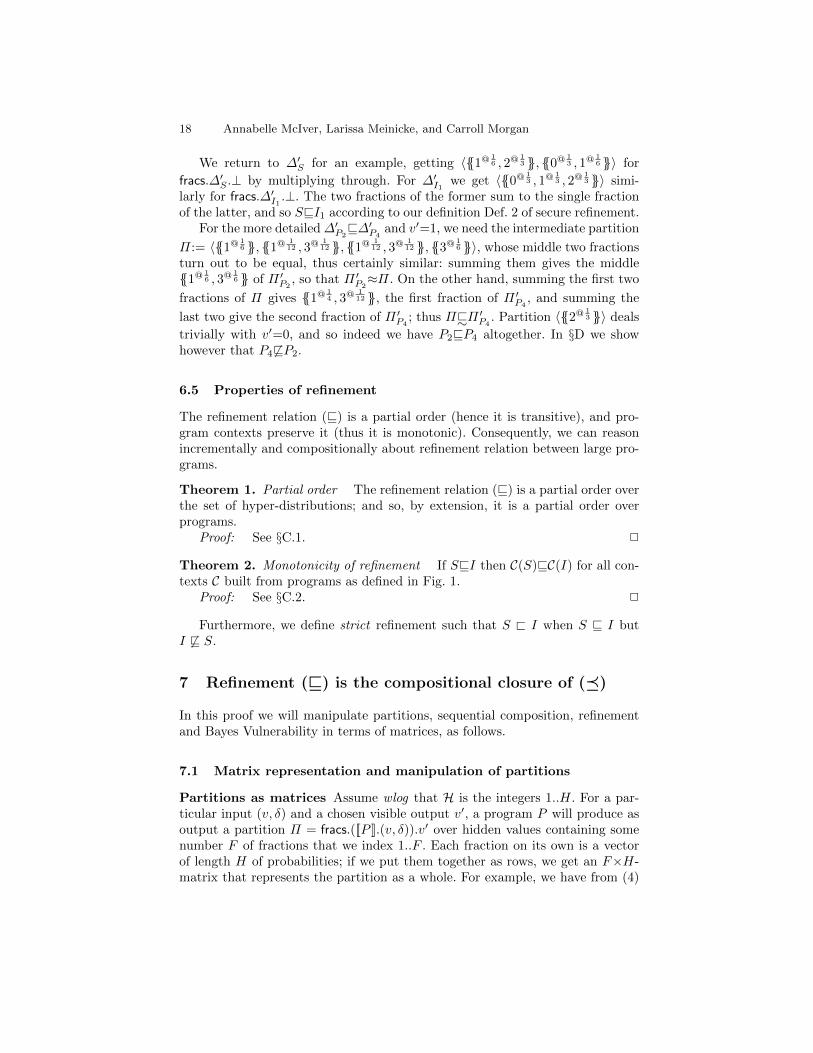
We return to ∆′S for an example, getting 〈{{1@ 16 , 2@ 1
3 }}, {{0@ 13 , 1@ 1
6 }}〉 for
fracs.∆′S .⊥ by multiplying through. For ∆′I1 we get 〈{{0@ 13 , 1@ 1
3 , 2@ 13 }}〉 simi-
larly for fracs.∆′I1 .⊥. The two fractions of the former sum to the single fractionof the latter, and so SvI1 according to our definition Def. 2 of secure refinement.
For the more detailed ∆′P2v∆′P4
and v′=1, we need the intermediate partition
Π:= 〈{{1@ 16 }}, {{1@ 1
12 , 3@ 112 }}, {{1@ 1
12 , 3@ 112 }}, {{3@ 1
6 }}〉, whose middle two fractionsturn out to be equal, thus certainly similar: summing them gives the middle{{1@ 1
6 , 3@ 16 }} of Π ′P2
, so that Π ′P2≈Π. On the other hand, summing the first two
fractions of Π gives {{1@ 14 , 3@ 1
12 }}, the first fraction of Π ′P4, and summing the
last two give the second fraction of Π ′P4; thus Π@∼Π
′P4
. Partition 〈{{2@ 13 }}〉 deals
trivially with v′=0, and so indeed we have P2vP4 altogether. In §D we showhowever that P4 6vP2.
6.5 Properties of refinement
The refinement relation (v) is a partial order (hence it is transitive), and pro-gram contexts preserve it (thus it is monotonic). Consequently, we can reasonincrementally and compositionally about refinement relation between large pro-grams.
Theorem 1. Partial order The refinement relation (v) is a partial order overthe set of hyper-distributions; and so, by extension, it is a partial order overprograms.
Proof: See §C.1. 2
Theorem 2. Monotonicity of refinement If SvI then C(S)vC(I) for all con-texts C built from programs as defined in Fig. 1.
Proof: See §C.2. 2
Furthermore, we define strict refinement such that S @ I when S v I butI 6v S.
7 Refinement (v) is the compositional closure of (�)
In this proof we will manipulate partitions, sequential composition, refinementand Bayes Vulnerability in terms of matrices, as follows.
7.1 Matrix representation and manipulation of partitions
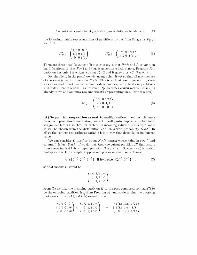
Partitions as matrices Assume wlog that H is the integers 1..H. For a par-ticular input (v, δ) and a chosen visible output v′, a program P will produce asoutput a partition Π = fracs.([[P ]].(v, δ)).v′ over hidden values containing somenumber F of fractions that we index 1..F . Each fraction on its own is a vectorof length H of probabilities; if we put them together as rows, we get an F×H-matrix that represents the partition as a whole. For example, we have from (4)
Compositional closure for Bayes Risk in probabilistic noninterference 19
the following matrix representations of partitions output from Programs P{2,4}for v′=1:
Π ′P2:
1/6 0 01/6 0 1/6
0 0 1/6
Π ′P4:
(1/4 0 1/12
1/12 0 1/4
). (5)
There are three possible values of h in each case, so that H=3; and P2’s partitionhas 3 fractions, so that F2=3 and thus it generates a 3×3 matrix. Program P4’spartition has only 2 fractions, so that F4=2 and it generates a 2×3 matrix.
For simplicity in the proof, we will arrange that H=F so that all matrices areof the same (square) dimension N×N . This is without loss of generality, sincewe can extend H with extra, unused values; and we can extend our partitionswith extra, zero fractions. For instance Π ′P4
becomes a 3×3 matrix, as Π ′P2is
already, if we add an extra row underneath (representing an all-zero fraction):
Π ′P4:
1/4 0 1/12
1/12 0 1/4
0 0 0
. (6)
(A) Sequential composition as matrix multiplication In our completenessproof, our program-differentiating context C will post-compose a probabilisticassignment h:∈D.h so that, for each of its incoming values h, the output valueh′ will be chosen from the distribution D.h, thus with probability D.h.h′. Ineffect the context redistributes variable h in a way that depends on its currentvalue.
We can consider D itself to be an N×N matrix whose value in row h andcolumn h′ is just D.h.h′. If we do that, then the output partition Π ′ that resultsfrom executing h:∈D.h on input partition Π is just Π×D, where (×) is matrixmultiplication. For example, suppose our post-composed context were
h:∈ ( {{1@ 12 , 2@ 1
4 , 3@ 14 }} if h=1 else {{2@ 1
2 , 3@ 12 }} ) , (7)
so that matrix D would be 1/2 1/4 1/4
0 1/2 1/2
0 1/2 1/2
.
From (5) we take the incoming partition Π to the post-composed context (7) tobe the outgoing partition Π ′P2
from Program P2, and so determine the outgoingpartition Π ′ from (P ′2; h:∈D.h) overall to be 1/6 0 0
1/6 0 1/6
0 0 1/6
× 1/2 1/4 1/4
0 1/2 1/2
0 1/2 1/2
=
1/12 1/24 1/24
1/12 1/8 1/8
0 1/12 1/12
.

20 Annabelle McIver, Larissa Meinicke, and Carroll Morgan
(B) Refinement as matrix multiplication Also refinement can be formu-lated as matrix multiplication, since it is essentially a rearranging of fractionswithin a partition that, therefore, boils down to rearrangement of rows withina matrix. For example, from §6.4 we recall that to refine Π ′P2
into Π ′P4we split
the middle fraction of the former into two equal pieces, and add them to theother two, and that is achieved by the left-hand matrix in the pre-multiplicationshown here: 1 1/2 0
0 1/2 10 0 0
× 1/6 0 0
1/6 0 1/6
0 0 1/6
=
1/4 0 1/12
1/12 0 1/4
0 0 0
.
In general a partition ΠS is refined by ΠI iff there exists a refinement matrixR, a matrix whose columns are non-negative and one-summing, such that R×ΠS
equals ΠI . Entry (r, c) of such a refinement matrix describes what proportion ofthe cth fraction (row) of ΠS is to contribute by addition to the rth fraction ofΠI .
(C) Bayes Vulnerability as matrix multiplication Finally we bring BayesVulnerability into the matrix algebra as well. For a partition Π as a matrix, thevulnerability is found by taking the individual row maxima and adding themtogether: the result is a scalar. Thus for Π ′P4
, for example, we have the matrix 1/4 0 1/12
1/12 0 1/4
0 0 0
with maxima selected by the strategy matrix G:
1 0 00 0 10 0 1
whose maxima have been set in bold and are selected by the 1 entries in thematrix G at right. Note that strategy matrices have the same shape as thematrix from which they select, and that they are 0/1 matrices with exactly one1 per row. 17
To determine the vulnerability associated with the Π, we calculate
(t strategy matrices G · tr.(GT×Π)) (8)
in general, where (·)T is matrix transpose and tr takes the trace of a squarematrix, i.e. the sum of its diagonal. Note that the maximum is actually attained,for some G, since there are only finitely many of them. In this particular casewe use the G above to calculate tr.(GT×Π ′P4
), and have therefore1 0 00 0 00 1 1
× 1/4 0 1/12
1/12 0 1/4
0 0 0
=
1/4 0 1/12
0 0 01/12 0 1/4
,
whose trace is 1/4 + 0 + 1/4 = 1/2 to give the Bayes Vulnerability of Π ′P4.
17 Of course in an all-zero row it makes no difference which entry is selected.

Compositional closure for Bayes Risk in probabilistic noninterference 21
(D) The connection between strategy matrices and refinement For anystrategy matrix G, the transpose GT has exactly one 1 in each column, and thuscan be regarded as a simple refinement matrix, one of those which (when pre-multiplied with a partition) merges only whole fractions. If we denote the set ofN×N strateGy matrices by GN , the set of N×N Refinement matrices by RN ,and the siMple subset of these (having only one non-zero entry per row) byMN , we thus have that
{G:GN · GT} = MN ⊆ RN .
Furthermore, it can be shown that the complete set of refinement matrices RNis in fact the convex closure of its simple subset:
RN = ccl.(MN ) . (9)
From (8) and by linearity of matrix operations multiplication and trace, we thushave for any N×N -dimensional Π that the Bayes Vulnerability is given by
bv.Π = (tG:GN · tr.(GT×Π)) = (tR:RN · tr.(R×Π)) , (10)
because the extra elements in RN but not GNT are only interpolations, and socannot increase the maximum of a linear expression. (Recall from above thatthis maximum is attained for some R.)
Additionally, RN forms a monoid under matrix multiplication, that is
(RN ,×,1N ) is a monoid, (11)
where 1N is the N×N unit of matrix multiplication. 18 We refer to §A for aproof of Properties (9) and (11).
7.2 Soundness
Here from SvI we must show that C(S)�C(I) for all contexts C. From mono-tonicity (Thm. 2) it suffices to show that SvI implies S�I.
Fix an initial split-state and construct the output hyper-distributions ∆′{S,I}that result from S, I respectively. Then since we assume SvI we must have∆′Sv∆′I . We now show that this implies ∆′S�∆′I .
Since SvI trivially guarantees that ft.∆′S = ft.∆′I –recall Def. 2– we needto show that the Bayes-Vulnerability condition in the elementary testing or-der is satisfied. Since bv.∆ = (
∑v:V · bv.(fracs.∆.v)) , it is enough to show
that for each v:V the vulnerability of Π ′S := fracs.∆′S .v is no less than that ofΠ ′I := fracs.∆′I .v.
For any such Π ′{S,I} assume wlog that they are represented as N×N matrices.We then have that
18 Note that it is not a group because only the matrices in RN that permute –but donot combine– fractions have inverses.

22 Annabelle McIver, Larissa Meinicke, and Carroll Morgan
bv.Π ′S= (tR:RN · tr.(R×Π ′S)) . “from (D), Property (10)”
= (tR1, R2:RN · tr.(R1×R2×Π ′S) ) “from (D), Property (11)”
≥ (tR1:RN · tr.(R1×R2×Π ′S) ) “for any R2”
= (tR1:RN · tr.(R1×Π ′I)) . “from (B), choose R2 so that R2×Π ′S = Π ′I”
= bv.Π ′I . “from (D), Property (10)”
That gives us
Theorem 3. Refinement is sound for Bayes Risk If SvI then C(S)�C(I)for all contexts C. 2
7.3 Completeness
Here from S 6vI we must discover a context C such that C(S) 6�C(I). (The proofhere is self-contained; but as background we give a fully worked example in §D).
Since S 6vI, there must be an initial split-state (v, δ) from which S, I yieldhyper-distributions ∆′{S,I} with ∆′S 6v∆′I . We can assume however that ∆′S,Igive equal overall probabilities to visible variables since, if they did not, theywould be functionally different, giving S 6�I immediately. This being so, we canassume that for some final v′ we have that partition ΠS := fracs.∆′S .v
′ cannot betransformed into partition ΠI := fracs.∆′I .v
′ via the two steps (i), (ii) in Def. 2.That is, we have ΠS 6v ΠI .
We will define a distribution D such that the context (− ; C) where C is
if v=v′ then h:∈D.h else h:= 0 fi
can be used to differentiate S from I using elementary testing.We dispose of the simple case first: if v′′ 6=v′ then fracs.([[S;C]].(v, δ)).v′′ equals
fracs.([[I;C]].(v, δ)).v′′ since, first, hyper-distributions ∆′{S,I} give equal proba-bilities to that v′′ and, second, the final value h′ of h is zero for both S;C andI;C in that case. The vulnerability associated with these partitions is thereforethe same. To establish [[S;C]] 6� [[I;C]] for our chosen C, it is thus enough toshow that the vulnerability of fracs.([[I;C]].(v, δ)).v′ is strictly greater than forfracs.([[S;C]].(v, δ)).v′. Treating Π{S,I} as N×N matrices, we calculate
“Bayes Vulnerability of ΠS ;C ”= “Bayes Vulnerability of ΠS×D ” “(A) above; definition of C based on D ”
= tr.(R×ΠS×D) “(10) in (D) above; for some maximising R∈RN”
= tr.(Π×D) “(B) above; for refinement Π = R×ΠS of ΠS”
< tr.(ΠI×D) “D was chosen in advance, using the Separating
Hyperplane Lemma, and does not depend on Π: see below”
= tr.(1×ΠI×D) “identity”
≤ (tR:RN · tr.(R×ΠI×D)) “1∈RN”
= “Bayes Vulnerability of ΠI×D ” “(10) in (D) above”

Compositional closure for Bayes Risk in probabilistic noninterference 23
= “Bayes Vulnerability of ΠI ;C ” . “(A) above; definition of C ”
The structure of the argument is basically a reformulation on the S side, anappeal to the separation property of the “pre-selected” matrix D, and then acomplementary un-reformulation on the I side. Thus for “see below” we argueas follows.
To prepare D we consider all possible refinements of ΠS together. Theserefinements {{R:RN · R×ΠS}} comprise a convex set of N×N matrices, (whereconvexity follows from (9) and linearity of matrix multiplication). Since ΠI isnot a refinement of ΠS , we know ΠI is not in that set. If we “flatten out” thematrices into vectors of length N2, say by glueing their rows together, then wehave a “point” ΠI in Euclidean space that is strictly outside of that convex setand by the Separating Hyperplane Lemma [35] there must be a plane with normal
X that strictly separates that whole set of refinements (including Π = R×ΠS)from the single point ΠI . The point X too will be a vector of length N2 and,written with matrices, the strict-separation condition is then that
tr.(Π×XT) < tr.(ΠI×XT) for all Π refining ΠS
since the dot-product of two N2-vectors A,B written as matrices of size N×Nis just tr.(A×BT). This is precisely what we required above; and so our D ismade by taking the direction numbers of the separating hyperplane in EuclideanN2-space and turning them back into a matrix, and transposing the result.
We admit that there is no guarantee that the D constructed as above willhave one-summing rows. However, we can choose D to have all non-negativecoefficients because ΠI and all the refinements Π of ΠS have the same weight,and thus we can add any constant to all elements of D without affecting itsseparating property; similarly we can scale it by any positive number. Thus wecan assume wlog that D is non-negative and that all its rows sum to no morethan 1. To then make each row of D sum to one exactly we can extend it withan extra “column zero” whose entries are chosen just for that purpose. We thenneed to guarantee –as a technical detail– that neither the Bayes Vulnerabilitystrategy matrix for ΠS or ΠI chooses h to be zero. We do that, if necessary, byadding a second context program that acts as skip when h6=0; but when h=0 itexecutes a large probabilistic choice over h to distribute the 0 value over enoughnew values −1,−2 . . . to make sure none of them individually will have a largeenough probability to attract a maximising choice. 19 That gives us
Theorem 4. Refinement is complete for Bayes Risk If S 6vI then C(S)6�C(I)for some context C. 2
7.4 Maximal discrimination of the Bayes-Risk elementary order
In this section only, we write “�B” for the Bayes-Risk based elementary testingorder (�), and we write “�1” etc. to stand generically for any similar orderbased on one of the four alternative entropy measures set out in §1.2.
19 At most N new values will be required for such a context.
24 Annabelle McIver, Larissa Meinicke, and Carroll Morgan
The problem discussed in §1.2 was that one could have A≺1B and yet B≺2Afor programs A,B and competing elementary orders (�1) and (�2). Similarly,for any of the four (≺1) including (≺B) itself, it’s easy to manufacture exampleswhere we have A≺1B but there is a context C that reverses the comparison, sothat C(B)≺1C(A). This seems a hopelessly confused situation.
Luckily it turns out (§G) that refinement (v) is sound not only for (�B) butfor the other three orders as well and –since (v) is complete for Bayes Risk–that gives us
Theorem 5. Bayes Risk is maximally discriminating With context, BayesRisk is maximally discriminating among the orders of §1.2: that is if (�1) is anorder derived from one of the entropies of §1.2, then whenever for two programsS, I and all contexts C we have C(S)�BC(I) we also have C(S)�1C(I) for all C.
Equivalently, if two programs A,B are distinguished by any (�1) from §1.2,that is A 6�1B, then there is a context C such that (�B) in particular distinguishesC(A) and C(B), that is such that C(A) 6�BC(B).
Proof: The equivalence of the first and second formulations is straightfor-ward; 20 we prove the second, reasoning
A 6�1B⇒ A 6vB “soundness of (v) for (�1), see §G”
⇒ C(A) 6�BC(B) . “completeness of (v) for (�B); some context C”
2
It’s the completeness result for (�B) that makes it maximal, i.e. that seemsto single it out from among the other orders. Whether or not the other ordersare also complete is an open problem.
8 Case study: The Three Judges protocol
The motivation for our case study is to suggest and illustrate techniques for rea-soning compositionally from specification to implementation of noninterference[27, 23, 11]. Our previous examples include (unboundedly many) Dining Cryptog-raphers [6], Oblivious Transfer [32] and Multi-Party Shared Computation [39].All of them however used our qualitative model for compositional noninterference[27, 23]; here of course we are using instead a quantitative model.
20 First implies second:
If A6�1B then, appealing to the identity context in the conclusion of the firstformulation, for some C we have C(A) 6�BC(B).
Second implies first:
Assume C(S) 6�1C(I) for some C, whence immediately from the second formu-lation we have D(C(S)) 6�BD(C(I)) for some context D(C(·)).
Compositional closure for Bayes Risk in probabilistic noninterference 25
The example is as follows. Three judges A,B,C are to give a majority deci-sion, innocent or guilty, by exchanging messages but concealing their individualvotes a, b and c, respectively. 21
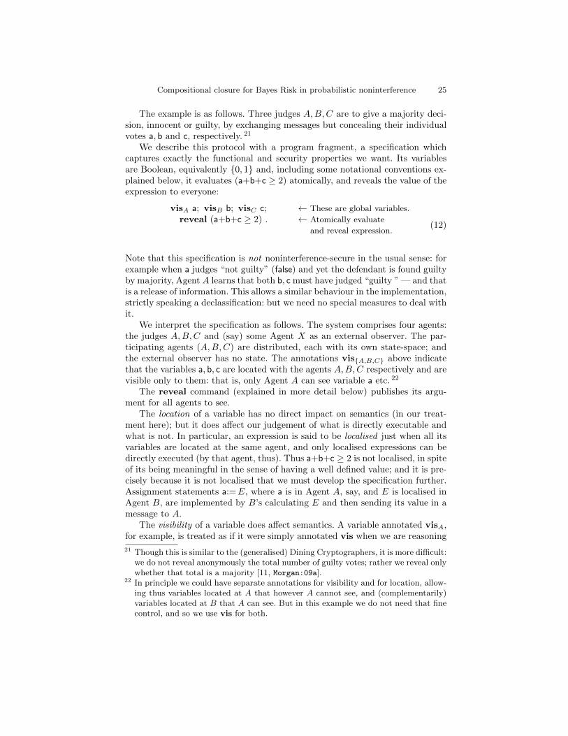
We describe this protocol with a program fragment, a specification whichcaptures exactly the functional and security properties we want. Its variablesare Boolean, equivalently {0, 1} and, including some notational conventions ex-plained below, it evaluates (a+b+c ≥ 2) atomically, and reveals the value of theexpression to everyone:
visA a; visB b; visC c; ← These are global variables.
reveal (a+b+c ≥ 2) . ← Atomically evaluate
and reveal expression.(12)
Note that this specification is not noninterference-secure in the usual sense: forexample when a judges “not guilty” (false) and yet the defendant is found guiltyby majority, Agent A learns that both b, c must have judged “guilty ” — and thatis a release of information. This allows a similar behaviour in the implementation,strictly speaking a declassification: but we need no special measures to deal withit.
We interpret the specification as follows. The system comprises four agents:the judges A,B,C and (say) some Agent X as an external observer. The par-ticipating agents (A,B,C) are distributed, each with its own state-space; andthe external observer has no state. The annotations vis{A,B,C} above indicatethat the variables a, b, c are located with the agents A,B,C respectively and arevisible only to them: that is, only Agent A can see variable a etc. 22
The reveal command (explained in more detail below) publishes its argu-ment for all agents to see.
The location of a variable has no direct impact on semantics (in our treat-ment here); but it does affect our judgement of what is directly executable andwhat is not. In particular, an expression is said to be localised just when all itsvariables are located at the same agent, and only localised expressions can bedirectly executed (by that agent, thus). Thus a+b+c ≥ 2 is not localised, in spiteof its being meaningful in the sense of having a well defined value; and it is pre-cisely because it is not localised that we must develop the specification further.Assignment statements a:=E, where a is in Agent A, say, and E is localised inAgent B, are implemented by B’s calculating E and then sending its value in amessage to A.
The visibility of a variable does affect semantics. A variable annotated visA,for example, is treated as if it were simply annotated vis when we are reasoning
21 Though this is similar to the (generalised) Dining Cryptographers, it is more difficult:we do not reveal anonymously the total number of guilty votes; rather we reveal onlywhether that total is a majority [11, Morgan:09a].
22 In principle we could have separate annotations for visibility and for location, allow-ing thus variables located at A that however A cannot see, and (complementarily)variables located at B that A can see. But in this example we do not need that finecontrol, and so we use vis for both.

26 Annabelle McIver, Larissa Meinicke, and Carroll Morgan
from Agent A’s point of view; from Agents’ B,C points of view, it is treated asif it were annotated hid; and the same applies analogously to the other agents.Thus in the example we will treat three agents A,B,C each with her own view:variables visible to one (declared vis) will be hidden from another (declared hid)— and vice versa. The “extra” Agent X (mentioned above) sees none of a, b, c,but does observe the reveal. This simple approach is possible for us becausewe are not dealing with agents whose actions can be influenced by other agents’knowledge.
In principle the vis-subscripting convention means that protocol develop-ment, e.g. as in §8.3ff. to come, will require a separate proof for each observer(since the patterns of variables’ visibility might differ); but in practice we canusually find a single chain of reasoning each of whose steps is valid for two oreven all three observers at once.
Before incrementally developing (12) into an implementation in order to lo-calise its expressions, we introduce some further extensions, including the revealstatement mentioned above [22], that will be used in the subsequent programderivation.
8.1 Further program-language extensions
Multiple- and local variables To this point we have had just two variables,visible v and hidden h, and a split-state V×DH to describe their behaviour. Inpractice each of V,H will each comprise many variables, represented in the usualCartesian way. Thus if we have variables a:A, b:B, c: C, d:D with the first twoa, b visible and the last two c, d hidden, then V is A×B and H is C×D so thatthe state-space is A×B×D(C×D). Assignments and projections are handled asnormal.
We allow local variables, both visible and hidden, which are treated (also) asnormal: within the scope of a visible local-variable declaration ‖[ vis x:X · · · ]‖,the Vlocal used is X×Vglobal. Hidden variables are treated similarly.23
Revelations Command reveal E publishes expression E for all to see: it isequivalent to the local block
‖[ vis v; v:=E ]‖ , (13)
but it avoids the small extra complexity of declaring the temporary visible-to-all variable v and the having to introduce the scope brackets as (13) does.The attraction of this is that the reveal command has a simple algebra of itsown, including for example that reveal E = reveal F just when E and Fare interdeducible given the values of (other) visible variables [22, 24]. Thus forexample (and slightly more generally) we have
reveal a∇b; reveal b∇c = reveal b∇c; reveal c∇a ,23 Implicitly local variables are assumed to be initialised by a uniform choice over
their finite state space. In our examples however, we always initialize local variablesexplicitly, to avoid confusion.
Compositional closure for Bayes Risk in probabilistic noninterference 27
using (∇) to denote exclusive-or, because from a∇b and b∇c an observer candeduce both b∇c and c∇a, and vice versa.
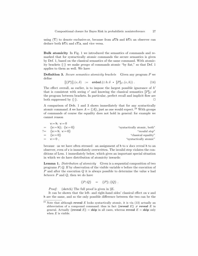
Bulk atomicity In Fig. 1 we introduced the semantics of commands and re-marked that for syntactically atomic commands the secure semantics is givenby Def. 1, based on the classical semantics of the same command. With atomic-ity brackets 〈〈·〉〉 we make groups of commands atomic “by fiat,” so that Def. 1applies to them as well. We have
Definition 3. Secure semantics atomicity brackets Given any program P wedefine
[[〈〈P 〉〉]].(v, δ) := embed.(�h: δ · [[P ]]C .(v, h)) . (14)
The effect overall, as earlier, is to impose the largest possible ignorance of h′
that is consistent with seeing v′ and knowing the classical semantics [[P ]]C ofthe program between brackets. In particular, perfect recall and implicit flow areboth suppressed by 〈〈·〉〉. 2
A comparison of Defs. 1 and 3 shows immediately that for any syntacticallyatomic command A we have A = 〈〈A〉〉, just as one would expect. 24 With groupsof commands of course the equality does not hold in general: for example wecannot reason
v:= h; v:= 0= 〈〈v:= h〉〉; 〈〈v:= 0〉〉 “syntactically atomic, both”
?= 〈〈v:= h; v:= 0〉〉 “invalid step”
= 〈〈v:= 0〉〉 “classical equality”
= v:= 0 , “syntactically atomic”
because –as we have often stressed– an assignment of h to v does reveal h to anobserver, even of v is immediately overwritten. The invalid step violates the con-ditions of Lem. 1 immediately below, which gives an important special situationin which we do have distribution of atomicity inwards:
Lemma 1. Distribution of atomicity Given is a sequential composition of twoprograms P ;Q. If by observation of the visible variable v before the execution ofP and after the execution Q it is always possible to determine the value v hadbetween P and Q, then we do have
〈〈P ;Q〉〉 = 〈〈P 〉〉; 〈〈Q〉〉 .
Proof: (sketch) The full proof is given in §E.It can be shown that the left- and right-hand sides’ classical effect on v and
h are the same, and so the only possible difference between the two can be the
24 Note that although reveal E looks syntactically atomic, it is via (13) actually anabbreviation of a compound command: thus in fact 〈〈reveal E〉〉 6= reveal E ingeneral. Actually 〈〈reveal E〉〉 = skip in all cases, whereas reveal E = skip onlywhen E is visible.

28 Annabelle McIver, Larissa Meinicke, and Carroll Morgan
degree to which h is hidden. On the left, variable h must be maximally hiddensince that is the (defined) effect of the atomicity brackets 〈〈·〉〉. Thus we needonly argue that h is maximally hidden on the right as well.
Since h is maximally hidden after 〈〈P 〉〉, the only way h can fail to be max-imally hidden after the subsequent 〈〈Q〉〉 is if there are two (or more) distinctvalues of v after P , say v{0,1} each with its associated hidden distribution δ{0,1}of h, that are brought together to the same final value v′ by execution of Q. Forthat would mean that after Q we could have two distinct distributions δ′{0,1}of h associated with that single v′, which is precisely what it means not to bemaximally hidden. Each δ′{0,1} would have been derived from the correspondingδ{0,1} in between.
That scenario cannot occur if for any particular starting v before P that leadsto two (or more) values v{0,1} between P and Q, we never have Q bringing thosevalues back together again to a single final value v′. That amounts to being ableto determine the intermediate value v of v from its values before (v) and after(v′). 2
In fact our invalid step 〈〈v:= h; v:= 0〉〉 6= 〈〈v:= h〉〉; 〈〈v:= 0〉〉 above shows off thecondition exactly. Although v’s intermediate value is indeed determined by theinitial h, that is not good enough because we cannot see that h: we have accessonly to the initial v. And v’s final value is always 0, again hiding v’s intermediatevalue from us. Knowing v before and after, in this example, does not tell us itsintermediate value (which is in fact h).
By definition, semantic equivalence of P and Q in the classical model entailssemantic equivalence of 〈〈P 〉〉 and 〈〈Q〉〉 — that is why within atomicity bracketswe can use classical equality reasoning.
8.2 Subprotocols: qualitative vs. quantitative reasoning
Rather than appeal constantly to the basic semantics (Fig. 1) instead we haveaccumulated, with experience, a repertoire of identities –a program algebra–which we use to reason at the source level. Those identities themselves are proveddirectly in the semantics but, after that, they become permanent members ofthe designer’s toolkit. One of the most common is the Encryption Lemma.
The Encryption Lemma Let statement (v∇h):=E set Booleans v, h so thattheir exclusive-or v∇h equals Boolean E: there are exactly two possible waysof doing so. In our earlier work [27], we proved that when the choice is madedemonically, on a single run nothing is revealed about E; in our refinement stylewe express that as
skip = ‖[ vis v; hid h; (v∇h):=E ]‖ . (15)
In our current model we can prove that exactly the same identity holds providedthe choice of possible values for v and h is made uniformly:

Compositional closure for Bayes Risk in probabilistic noninterference 29
Lemma 2. The Encryption Lemma For any Boolean expression E we havethat the following block is equal to skip, and so reveals nothing:
‖[ vis v; hid h; (v∇h):=E ]‖ .
For this we require that the implicit choice in (v∇h):=E is made uniformly.Proof: We calculate
‖[ vis v; hid h; (v∇h):=E ]‖= ‖[ vis v; hid h; 〈〈(v∇h):=E〉〉 ]‖ “syntactically atomic”
= ‖[ vis v; hid h; 〈〈v:= true⊕false; h:= v∇E〉〉 ]‖ “classical equality (†)”= ‖[ vis v; hid h; 〈〈v:= true⊕false〉〉; 〈〈h:= v∇E〉〉 ]‖ “Lem. 1”
= ‖[ vis v; hid h; v:= true⊕false; h:= v∇E ]‖ “syntactically atomic”
= ‖[ vis v; v:= true⊕false; ‖[ hid h; h:= v∇E ]‖ ]‖ “hid h does not capture”
= ‖[ vis v; v:= true⊕false ]‖ “assignment to local hidden is skip”
= skip . “value assigned to local v is known already (‡)”
2
The crucial step in the proof above was the classical equality at (†), and wenote that other variations are possible: for example we also have the classicalequality
(v∇h):=E = h:= true⊕false; v:=E∇h , (16)
which suggests the operational procedure of “flipping a private coin h ” and thenrevealing (via assignment to local v) the exclusive-or of that private coin withsome expression E. The above reasoning shows that also to be equal to skip.
Finally, we recall that (⊕) means choose uniformly, and we now show thatit is essential for the (†) step and for the equality (16): if for example we hadh:= true p⊕ false; v:=E∇h in (16) on the right-hand side, but with p6=1/2, itwould not be possible to rewrite that in the form v:= true 1/2⊕ false; h:= v∇E aswe had at (†) but with the 1/2 here exposed. Instead we’d have
v:=¬Ep⊕E; h:= v∇E
and the last step (‡) would then be invalid if E contained hidden variables (asit usually would). The role of p=1/2 is thus that the equality
v:=¬E 1/2⊕ E = v:= true 1/2⊕ false
holds no matter what expression E is, and in particular even if it contains hiddenvariables — but only (in general) when the choice is with probability 1/2.
Lem. 2 means that extant qualitative source-level proofs that rely only on“upgradeable identities” like (15) can be used as is for quantitative results pro-vided the demonic choices involved are converted to uniform choice. And that isthe case with our current example.
Beyond the Encryption Lemma, we use Two-party Conjunction [39] andOblivious Transfer [32] in our implementation. Just as for the Encryption Lemma,the algebraic proofs of their implementations [27, 23] apply quantitatively pro-vided we interpret the (formerly) demonic choice as uniform. We now look brieflyat those subprotocols.
30 Annabelle McIver, Larissa Meinicke, and Carroll Morgan
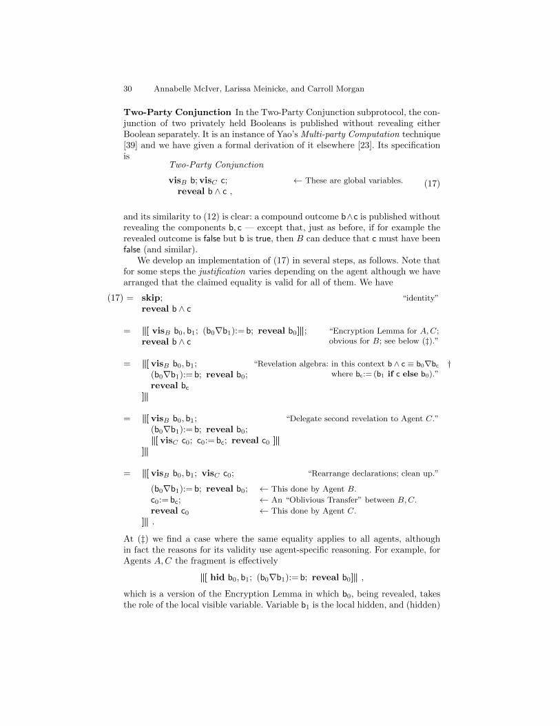
Two-Party Conjunction In the Two-Party Conjunction subprotocol, the con-junction of two privately held Booleans is published without revealing eitherBoolean separately. It is an instance of Yao’s Multi-party Computation technique[39] and we have given a formal derivation of it elsewhere [23]. Its specificationis
Two-Party Conjunction
visB b; visC c; ← These are global variables.
reveal b ∧ c ,(17)
and its similarity to (12) is clear: a compound outcome b∧c is published withoutrevealing the components b, c — except that, just as before, if for example therevealed outcome is false but b is true, then B can deduce that c must have beenfalse (and similar).
We develop an implementation of (17) in several steps, as follows. Note thatfor some steps the justification varies depending on the agent although we havearranged that the claimed equality is valid for all of them. We have
(17) = skip;reveal b ∧ c
“identity”
= ‖[ visB b0, b1; (b0∇b1):= b; reveal b0]‖;reveal b ∧ c
“Encryption Lemma for A,C;obvious for B; see below (‡).”
= ‖[ visB b0, b1;(b0∇b1):= b; reveal b0;reveal bc
]‖
“Revelation algebra: in this context b ∧ c ≡ b0∇bc †where bc:= (b1 if c else b0).”
= ‖[ visB b0, b1;(b0∇b1):= b; reveal b0;‖[ visC c0; c0:= bc; reveal c0 ]‖
]‖
“Delegate second revelation to Agent C.”
= ‖[ visB b0, b1; visC c0;
(b0∇b1):= b; reveal b0; ← This done by Agent B.
c0:= bc; ← An “Oblivious Transfer” between B,C.
reveal c0 ← This done by Agent C.
]‖ .
“Rearrange declarations; clean up.”
At (‡) we find a case where the same equality applies to all agents, althoughin fact the reasons for its validity use agent-specific reasoning. For example, forAgents A,C the fragment is effectively
‖[ hid b0, b1; (b0∇b1):= b; reveal b0]‖ ,
which is a version of the Encryption Lemma in which b0, being revealed, takesthe role of the local visible variable. Variable b1 is the local hidden, and (hidden)

Compositional closure for Bayes Risk in probabilistic noninterference 31
variable b is the expression E (on which there are no restrictions). On the otherhand, for Agent B the fragment is
‖[ vis b0, b1; (b0∇b1):= b; reveal b0]‖
with b a global visible: this is trivially equal to skip because all variables arevisible.
At (†) we use the revelation algebra mentioned in §8.1 to reason that onceb0 is revealed, going on to reveal b ∧ c is equivalent to revealing just bc since–knowing b0– we can calculate each of b ∧ c and bc from the other. 25
More interesting than any of that, however, is that in the last step we ap-peal to a further subprotocol by including the specification of the “ObliviousTransfer Protocol” [31, 32]. Here Agent C has a private {0, 1}-valued variable cand obtains from Agent B either b0 or b1, depending on c. But Agent B doesnot discover what c is, and Agent C does not discover b¬c. We give a rigorousimplementation of the protocol elsewhere [27]; an informal explanation may befound in §F.
Finally, to emphasise our earlier point about declassification, we suppose b istrue but c is false and thus that B learns c by noting that false is revealed overall;note that this is a property of the specification. Now, in the implementation,we can see how this happens: when b is true the local variables b0,1 will becomplementary and so –in spite of not learning c while the Oblivious Transfer iscarried out– Agent B will still learn c afterwards by comparing c0 with her ownb0,1.
8.3 The Three-Judges implementation: first attempt
We begin with an implementation attempt that fails, because this will illustratetwo things. The first is that our model prevents incorrect developments, that is itstops us from constructing implementations less secure than their specifications:arguably this “negative” aspect of a method is its most important property, sinceit would be trivial to describe a method that allowed secure refinements. . . andall others as well. The key is what is not allowed.
The second thing illustrated here is that a conditional if E · · · fi should beconsidered to reveal its condition E implicitly. This implicit flow is a propertyforced upon us by our advocacy of program algebra and our use of composition-ality: since the then- and the else branch of a conditional can be developeddifferently after the conditional has been introduced, we must expect that thosedifferences might reveal to an attacker which branch is being executed (and hencethe condition implicitly). This is exactly what we are about to see.
25 We have
b0∇bc ≡ (b0∇b1 if c else b0∇b0) ≡ (b if c else false) ≡ b ∧ c .

32 Annabelle McIver, Larissa Meinicke, and Carroll Morgan
We start with some Boolean algebra
(a+b+c ≥ 2) ≡ a ∧ (b ∨ c) ∨ b ∧ c ≡ (b ∨ c if a else b ∧ c) ,
and that suggests the first development steps
reveal (a+b+c ≥ 2)
?=
if a then reveal (a+b+c ≥ 2)else reveal (a+b+c ≥ 2)
fi
“P?= if E then P else P fi”
= if athen reveal b ∨ celse reveal b ∧ c
fi . . .
“After then we can assume a;after else we can assume ¬a.”
(18)
Now we can deal immediately with the else-part by adapting the Two-PartyConjunction Protocol of §8.2 so that it reveals b∧c only to Agent A; we introducea pair of A-private local variables for that purpose. The result is
. . . = ‖[ visA aB , aC ; visB b0, b1; visC c0;
if athen reveal b ∨ celse (b0∇b1):= b; ← Done privately by Agent B.
aB := b0; ← Message B→A.
c0:= bc; ← Oblivious Transfer B→C.
aC := c0; ← Message C→A.
reveal aB∇aC ← Agent A announces majority verdict.
fi]‖ . . .
“Adapting §8.2”
For the then-part we write b ∨ c as ¬(¬b ∧ ¬c) and adapt the else-partaccordingly; the effect overall turns out to be replacing the initial b by ¬b andchanging the following assignment. Once we factor out the common portion ofthe conditional, we have
. . . = ‖[ visA aB , aC ; visB b0, b1; visC c0;
if a then (b0∇b1):=¬b; aB := b1 else (b0∇b1):= b; aB := b0 fi;c0:= bc; aC := c0;reveal aB∇aC
]‖ .
“Using de Morgan”

Compositional closure for Bayes Risk in probabilistic noninterference 33
Now we see that the problem with going further is that Agent A must some-how arrange that B carries out either (b0∇b1):=¬b or (b0∇b1):= b, with thatarrangement depending on the value of A’s private variable a. Since B’s twopotential computations are different, there is no way this can occur without B’slearning the value of a in the process: this code is already incorrect.
Thus we must abandon this attempt, and admit that the questionable stepat (18) above was indeed wrong. In order to allow us to develop distributedimplementations, we make the (reasonable) assumption that each agent knowsthe code it is instructed to execute, with those instructions coming possibly fromanother agent. In this case Agent B must execute either (b0∇b1):=¬b; aB := b1
or (b0∇b1):= b; aB := b0, depending on the value of a which is supposed to bevisible only to Agent A.
Our semantics recognises implicit flow, and does not allow in general thetransformation of P into if E then P else P fi, for exactly this reason. 26
Similarly, a fragment a:= b; a:= c represents two messages, one B→A and thena second one C→A; with perfect recall we recognise that A can learn b byexamining a after the first message has arrived, but before the second.
8.4 The Three-Judges implementation: second attempt (sketch)
An “obvious” remedy for §8.3’s problem, that Agent B’s is aware of which pro-cedure she must follow, is to make B follow both procedures, speculatively: shedoes not know which one A will actually use.
The difficulty is now with Agent A, who learns both b∧c and b∨c. Althoughthose two values do not (always) determine b and c themselves, they do providestrictly more information to A than her knowing a and (a+b+c ≥ 2) would haveprovided on their own. 27 Thus this approach fails also.
Our attention is therefore drawn to arranging for B (and C) to do both two-party calculations, but then for A to get the results of only one of them. Thatleads naturally to the approach of the next section, a combination of two two-party computations (letting Agents B,C do both calculations) and two (more)oblivious transfers (letting Agent A learning about only one of them.) 28
8.5 The Three-Judges implementation: successful development
To repair the problem we encountered above we must arrange that Agents B,Cas far as possible carry out procedures independent of A’s variable a, in particular
26 In our related work for noninterference with demonic choice and without probability[26, 27], we give further arguments for this point of view, but based directly onprogram algebra. The extra feature there is that even classical programs have a non-trivial refinement relation; here, we have proper refinement only for secure programs.
27 If a and (a+b+c ≥ 2) are both false, then Agent A concludes ¬(b∧c), for whichthere are the three possibilities false/false, true/false, false/true. Agent A’s addition-ally knowing b ∨ c would eliminate at least one of those three.
28 The “more” refers to the fact that the two-party computations have oblivious trans-fers inside of them.

34 Annabelle McIver, Larissa Meinicke, and Carroll Morgan
so that calculations relating to b∨c and to b∧c both occur, irrespective of whichresult A actually needs.
To achieve this we need a slightly more general form of two-party computa-tion. We begin by introducing the specification of such a two-party conjunction,with its variables made local so that the introduced code is equivalent to skip:
reveal (a+b+c ≥ 2)
= ‖[ visB b0; visC c0; (b0∇c0):= b ∧ c; ]‖;reveal (a+b+c ≥ 2)
“Two-party conjunction”
From Agent A’s point of view, the introduced statement is trivially equivalentto skip: all assignments are to local variables that A cannot see. From AgentB,C’s points of view, it is equivalent to skip because it is an instance of theEncryption Lemma: each of those two agents can see only one of the two variablesassigned-to, and so learns nothing about the expression b ∧ c. 29
The statement (b0∇c0):= b ∧ c we have introduced is a more general formof two-party conjunction than the reveal b ∧ c we illustrated earlier in §8.2 —that is because the conjunction is not actually revealed, not yet; instead it issplit into two “shares,” one belonging to each party B,C. Since each party hasonly one share, the conjunction is not revealed at all at this stage. But thoseshares can be used as inputs to further two-party computations, while preservingthe security, and the contribution of the conjunction to a larger computation isrevealed at a later point.
The extra generality introduced by the shares does not cause us extra workhere, since we are using only the specification for our reasoning and that (we willsee) suffices. When we come to implement the general two-party conjunction inmore primitive terms, however, we would then have further work to do. We havegiven such an implementation elsewhere [23].
With exactly the same reasoning as above we can introduce two-party dis-junction and, with both conjunction and disjunction present, perform some re-organisation:
29 The following bogus counter-argument is an example of what having a careful defi-nition of equality and refinement helps us to avoid.
“Agent B might know that b is false, and then perhaps receive false also in b∧.She concludes that c∧ is also false, which is a leak since c∧ is supposed to be privateto C, invisible to B.”
In fact this is not a leak, because to judge it so we must refer to the specificationof this fragment. But that is simply skip and there is no c∧ declared there: therevealed variable is local to the implementation only.
That is, publishing the value of a hidden variable declared only in the im-plementation might look like a leak in the conventional interpretation –consider‖[ visC c; · · · ; reveal c ]‖ for example– but it is actually a leak only if that variablec has come to contain information (via assignments say in the “· · · ” portion) aboutother, more global hidden variables that were present in the specification, originally.Our semantics checks for that automatically.

Compositional closure for Bayes Risk in probabilistic noninterference 35
. . . = ‖[ visB b0; visC c0; (b0∇c0):= b ∧ c; ]‖;‖[ visB b1; visC c1; (b1∇c1):= b ∨ c; ]‖;reveal (a+b+c ≥ 2)
“Two-party disjunction”
= ‖[ visB b0, b1; visC c0, c1;
(b0∇c0):= b ∧ c;(b1∇c1):= b ∨ c;reveal (a+b+c ≥ 2)
]‖
“Reorganise declarations and scoping”
= ‖[ visB b0, b1; visC c0, c1;
(b0∇c0):= b ∧ c;(b1∇c1):= b ∨ c;reveal ba∇ca
]‖ . . .
“Boolean algebra”
Now since ba∇ca is revealed to everyone, and thus to A in particular, it doesno harm first to capture that value in variables of A, and then to have Agent Areveal those instead:
. . . = ‖[ visA aB , aC ;visB b0, b1;visC c0, c1;
(b0∇c0):= b ∧ c;(b1∇c1):= b ∨ c;(aB∇aC):= ba∇ca;reveal aB∇aC
]‖ . . .
“Introduce local private variables of A”
The point of using two variables a{B,C} rather than one is to be able to splitthe transmission of information B,C→A into two separate oblivious transfersB→A and C→A.
Thus the protocol boils down to three two-party computations: a conjunctionb∧c, a disjunction b∨c and an exclusive-or ba∇ca. The rhs of the last is actuallywithin an atomic conditional on a, that is (b0∇c0) if a=0 else (b1∇c1).
8.6 Two-party exclusive-or
Our final step is to split the two-party exclusive-or into two separate assignments.This is achieved by introducing a local shared variable h that is visible to B,Conly, i.e. not to A, and encrypting both hidden variables with it. Thus we takethe step
(aB∇aC):= ba∇ca

36 Annabelle McIver, Larissa Meinicke, and Carroll Morgan
= ‖[ visB,C h;h:= true ⊕ false;aB := ba∇h;aC := ca∇h
]‖ ,
justified trivially for B,C since the only assignments of non-constants are tovariables visible only to A. For A the justification comes from the the use ofclassical equality reasoning within a temporary atomicity block (refer Lem. 1):the effect of the two fragments above on aB , aC is identical, and there are nooverwritten visible values.
We will now show that in fact the extra variable h is not necessary: byabsorbing it into earlier statements, and with some rearrangement of scopes wecan rewrite our code at the end of §8.5 as
. . . = ‖[ visA aB , aC ; visB b0, b1; visC c0, c1; visB,C h;
h:= true ⊕ false;(b0∇c0):= b ∧ c;(b1∇c1):= b ∨ c;
aB := ba∇h;aC := ca∇h;reveal aB∇aC
]‖ . . .
where in fact we have moved the declaration and initialisation of h right tothe beginning. We now absorb it into the earlier two-party computations byintroducing temporarily variables b′{0,1} and c′{0,1} which correspond to theirunprimed versions except that they, too, are encrypted with h. That gives
. . . = ‖[ visA aB , aC ;visB b0, b1, b
′0, b′1;
visC c0, c1, c′0, c′1;
visB,C h;
h:= true ⊕ false;(b0∇c0):= b ∧ c; b′0, c
′0:= b0∇h, c0∇h;
(b1∇c1):= b ∨ c; b′1, c′1:= b1∇h, c1∇h;
aB := b′a; ← Note primes, justified by earlier.
aC := c′a; ← Assignments to b′{0,1}, c′{0,1}.
reveal aB∇aC ]‖ . . .
“Boolean reasoning”
where we have replaced the ba∇h and ca∇h at the end of the code with theirsimpler, primed versions where the encryption in built-in. Now we can rearrangethe statements using h so that not only h but also the unprimed b{0,1} and c{0,1}become auxiliary; that is, we have for the conjunction
(b0∇c0):= b ∧ c; b′0, c′0:= b0∇h, c0∇h

Compositional closure for Bayes Risk in probabilistic noninterference 37
‖[ visA aB , aC ; visB b0, b1; visC c0, c1;b0:= true ⊕ false;b1:= true ⊕ false;
c0:= (b∇b0 if c else b0);c1:= (¬b1 if c else b∇b1);aB := (b1 if a else b0);aC := (c1 if a else c0);
Four oblivious transfers.
reveal aB∇aC ]‖We replace the two Two-Party ’junctions by their implementations as oblivious trans-fers: each becomes two statements instead of one. The random flipping of bits b{0,1} isthen collected at the start.
The preservation of correctness is guaranteed by the compositionality of the securitysemantics.
Fig. 2. Three-Judges Protocol assuming Oblivious Transfers as primitives
= 〈〈 (b0∇c0):= b ∧ c; b′0, c′0:= b0∇h, c0∇h 〉〉 “introduce atomicity”
= 〈〈 (b′0∇c′0):= b ∧ c; b0, c0:= b′0∇h, c′0∇h 〉〉 “classical equality”
= (b′0∇c′0):= b ∧ c; b0, c0:= b′0∇h, c′0∇h , “remove atomicity”
and similarly for the disjunction. Removing the auxiliaries, and then applying atrivial renaming to get rid of the primes, we end up with
. . . = ‖[ visA aB , aC ; visB b0, b1; visC c0, c1;
(b0∇c0):= b ∧ c; ← Two-Party Conjunction (contains Oblivious Transfer).
(b1∇c1):= b ∨ c; ← Two-Party Disjunction (contains Oblivious Transfer).
aB := ba; ← Oblivious Transfer.
aC := ca; ← Oblivious Transfer.
reveal aB∇aC ]‖
“Consolidating the above”
which is precisely what we sought.In Fig. 2 we give the code with the (two) two-party computations instanti-
ated. In Fig. 3 we instantiate one of the (four) oblivious transfers.
9 Conclusion: a challenge and an open problem
We have investigated the foundations for probabilistic non-interference securityby proposing a semantics, and a refinement order between its programs, whichwe have demonstrated has connections with existing entropy-based measures.Especially it is related to Bayes Risk and we have given a soundness and com-pleteness result that establishes compositional closure.
Our approach has a general goal: to justify practical methods which supportaccurate analysis of programs operating in a context of probabilistic uncertainty.

38 Annabelle McIver, Larissa Meinicke, and Carroll Morgan
Starting from Fig. 2, we replace the specification of the first of its four oblivious trans-fers c0:= (b∇b0 if c else b0) by an implementation in elementary terms [23]:
‖[ visA aB , aC ; visB b0, b1; visC c0, c1;b0:= true ⊕ false;b1:= true ⊕ false;
‖[ visB m′0,m′1; visC c′,m′;
c′:= true ⊕ false;m′0:= true ⊕ false; m′1:= true ⊕ false;m′:=m′c′ ; ← Done in advance by trusted third party. †
visABC x, y0, y1; ← Note these are visible to all three agents.x:= c∇c′;y0:= b0∇m′x;y1:= b∇b0∇m′¬x;c0:= yc∇m′ ← Although yc is public, only Agent C knows m′. ‡
]‖;
c1:= (¬b1 if c else b∇b1);aB := (b1 if a else b0);aC := (c1 if a else c0);
Three more oblivious transfers,each one to beexpanded as above.
reveal aB∇aC ]‖
Each of the other three transfers would expand to a similar block of code, makingabout 40 lines of code in all. The Oblivious Transfer is formally derived elsewhere [27];an informal explanation is given in §F.
The preservation of correctness, under expansion, is again guaranteed by the composi-tionality of the security semantics.
Note that aside from the statement marked † (and its three other instances within thethree other, unexpanded oblivious transfers), all messages are wholly public because ofthe declarations vis x, y0, y1; that is, all the privacy needed is provided already by theexclusive-or’ing with hidden Booleans, as ‡ shows.The only private communications (†×4) are done with the aid of a trusted third party.As explained by Rivest [32, 27] this party’s involvement occurs only before the protocolbegins, and it is trusted not to observe any data exchanged subsequently between theagents; alternatively, the subsequent transfers can themselves be encrypted withoutaffecting the protocol’s correctness. (A trusted third party without these limitationswould implement trivially any protocol of this kind, simply by collecting the secretdata, processing it and then distributing the result.)
Fig. 3. Three-Judges Protocol in elementary terms
Abstraction underlies tractable analysis, but the results of such analyses becomerelevant only if the method of abstraction aptly preserves the properties intendedfor examination. The impact of this research is to show firstly that our refinementorder aptly characterises Bayes Risk, and secondly that the former discrepancies

Compositional closure for Bayes Risk in probabilistic noninterference 39
between Bayes Risk and other information orders can be rationalised by takingcontexts into account.
By taking a fresh point of view, we have related entropies that were formerlythought to be inconsistent. Furthermore, we highlight the similarities betweennon-interference (as defence against an adversary) and large-scale structuringtechniques (such as stepwise refinement and its associated information hiding[29]) for probabilistic systems. Both require a careful distinction between whatdata can be observed and what data must be protected; by observing that dis-tinction in the definition of abstraction, we allow the tractable analysis of prop-erties which rely on “secrecy” (on the one hand) or “probabilistic local state”(on the other). This unified semantic foundation opens up the possibility for auniform approach to the specification of security properties, along with othersafety-critical features, during system design [20].
These positive results now present a challenge and an open problem. Thechallenge is to find a model where all three features, probability, nondetermin-ism and hidden state, can reside together, and then an equivalence betweensemantic objects which respects an appropriate definition of testing. The pres-ence of nondeterminism would then include a treatment of distributed systemswith schedulers having a restricted view of the state [4]; that is because nondeter-minism can be interpreted either as underspecification, or as a range of decisionspresented to a scheduler. Within such a model we would be increasing the powerof the adversary to harvest information about the hidden state by increasing theexpressivity of the contexts she can create. It is an open problem whether thatincreased power is sufficient to make the various information-theoretic orders(Bayes Risk, Shannon Entropy, Marginal Guesswork etc.) equivalent or whetherthey remain truly distinct.
Related techniques
The use of information orders, such as those summarised in §1.2, to determinethe extent to which programs leak their secrets is widespread. Early work thattook this approach includes [25, 38, 13], and more recently it has been employedin [34, 15, 1, 7, 18]. One of the contributions of this paper is to show how thoseevaluations can be related by taking a refinement-oriented perspective. Composi-tionality plays a major role in our definition of refinement and we note that otherorders between probability distributions such as the “peakedness” introduced byDubois and Hullermeir [9] appear not to be compositional when generalised toour hyperdistributions.
More significant than the particular information order is the way that it isused in the analysis of programs. Our approach uses specifications to charac-terise permitted leaks, and a refinement order which ensures that for our choseninformation order (i.e. Bayes Risk), the implementation is at least as secure asits specification. An alternative mode is taken by Braun et al. [1]. Rather thanrestricting the elementary testing-relation (�) to a compositional subset (v),they identify the safe contexts Csafe such that I “�” Csafe(I). With our emphasis
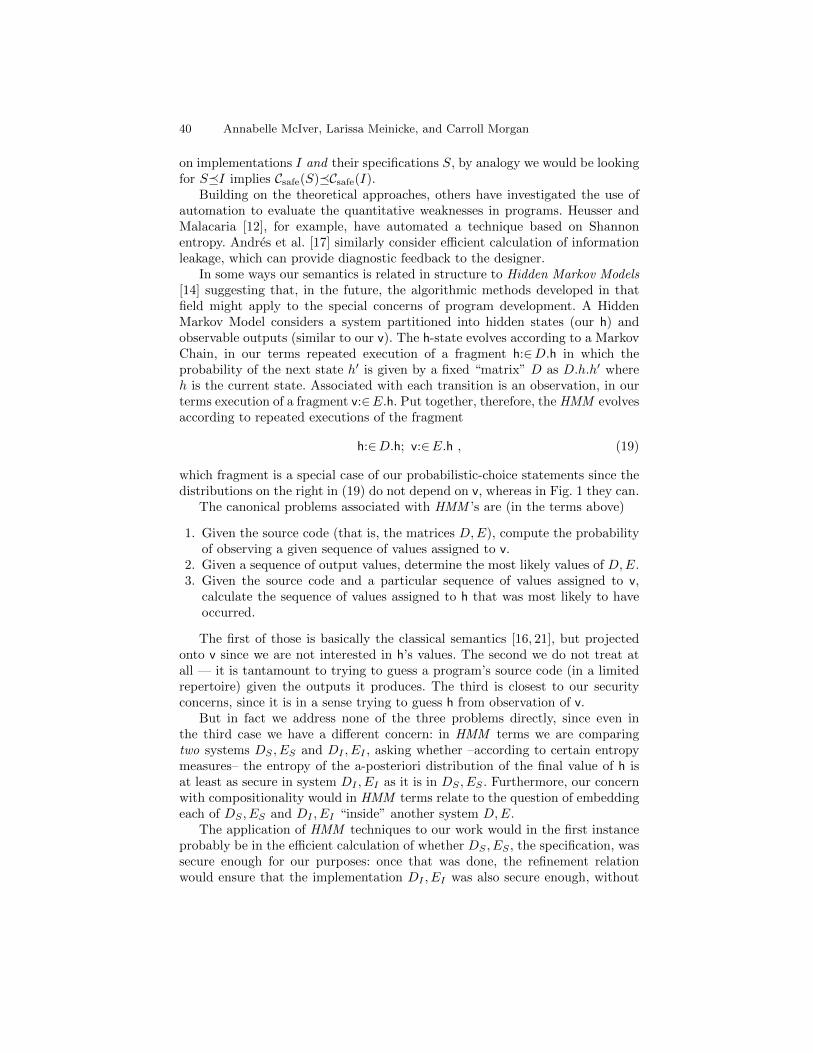
40 Annabelle McIver, Larissa Meinicke, and Carroll Morgan
on implementations I and their specifications S, by analogy we would be lookingfor S�I implies Csafe(S)�Csafe(I).
Building on the theoretical approaches, others have investigated the use ofautomation to evaluate the quantitative weaknesses in programs. Heusser andMalacaria [12], for example, have automated a technique based on Shannonentropy. Andres et al. [17] similarly consider efficient calculation of informationleakage, which can provide diagnostic feedback to the designer.
In some ways our semantics is related in structure to Hidden Markov Models[14] suggesting that, in the future, the algorithmic methods developed in thatfield might apply to the special concerns of program development. A HiddenMarkov Model considers a system partitioned into hidden states (our h) andobservable outputs (similar to our v). The h-state evolves according to a MarkovChain, in our terms repeated execution of a fragment h:∈D.h in which theprobability of the next state h′ is given by a fixed “matrix” D as D.h.h′ whereh is the current state. Associated with each transition is an observation, in ourterms execution of a fragment v:∈E.h. Put together, therefore, the HMM evolvesaccording to repeated executions of the fragment
h:∈D.h; v:∈E.h , (19)
which fragment is a special case of our probabilistic-choice statements since thedistributions on the right in (19) do not depend on v, whereas in Fig. 1 they can.
The canonical problems associated with HMM ’s are (in the terms above)
1. Given the source code (that is, the matrices D,E), compute the probabilityof observing a given sequence of values assigned to v.
2. Given a sequence of output values, determine the most likely values of D,E.3. Given the source code and a particular sequence of values assigned to v,
calculate the sequence of values assigned to h that was most likely to haveoccurred.
The first of those is basically the classical semantics [16, 21], but projectedonto v since we are not interested in h’s values. The second we do not treat atall — it is tantamount to trying to guess a program’s source code (in a limitedrepertoire) given the outputs it produces. The third is closest to our securityconcerns, since it is in a sense trying to guess h from observation of v.
But in fact we address none of the three problems directly, since even inthe third case we have a different concern: in HMM terms we are comparingtwo systems DS , ES and DI , EI , asking whether –according to certain entropymeasures– the entropy of the a-posteriori distribution of the final value of h isat least as secure in system DI , EI as it is in DS , ES . Furthermore, our concernwith compositionality would in HMM terms relate to the question of embeddingeach of DS , ES and DI , EI “inside” another system D,E.
The application of HMM techniques to our work would in the first instanceprobably be in the efficient calculation of whether DS , ES , the specification, wassecure enough for our purposes: once that was done, the refinement relationwould ensure that the implementation DI , EI was also secure enough, without

Compositional closure for Bayes Risk in probabilistic noninterference 41
requiring a second calculation. The advantage of this is that the first calculation,over a smaller and more abstract system, is likely to be much simpler than thesecond would have been.
References
1. C. Braun, K. Chatzikokolakis, and C. Palamidessi. Compositional methods forinformation-hiding. In Proc. FOSSACS’08, volume 4962 of LNCS, pages 443–57.Springer, 2008.
2. C. Braun, K. Chatzikokolakis, and C. Palamidessi. Quantitative notions of leakagefor one-try attacks. In Proc. MFPS, volume 249 of ENTCS, pages 75–91. ElsevierScience Publishers B. V., 2009.
3. Christian Cachin. Entropy measures and unconditional security in cryptography.PhD thesis, ETH, Zurich, Switzerland, 1997.
4. K. Chatzikokolakis and C. Palamidessi. Making random choices invisible to thescheduler. Information and Computation, 208(6):694–715, 2010.
5. K. Chatzikokolakis, C. Palamidessi, and P. Panangaden. Probability of error ininformation-hiding protocols. In Proc. CSF, pages 341–354. IEEE Computer So-ciety, 2007.
6. D. Chaum. The Dining Cryptographers problem: Unconditional sender and recip-ient untraceability. Jnl Cryptol., 1(1):65–75, 1988.
7. M.R. Clarkson, A.C. Myers, and F.B. Schneider. Quantifying information flowwith beliefs. Journal of Computer Security, 17(5):655–701, 2009.
8. M. de Nicola and M. Hennessy. Testing equivalence for processes. Theo Comp Sci,34:83–133, 1984.
9. D. Dubois and E. Hullermeier. A notion of comparative probabilistic entropy basedon the possibilistic specificity ordering. In Symbolic and Quantitative Approachesto Reasoning with Uncertainty, volume 3571 of LNCS, pages 848–859. Springer,2005.
10. J.A. Goguen and J. Meseguer. Unwinding and inference control. In Proc. IEEESymp on Security and Privacy, pages 75–86. IEEE Computer Society, 1984.
11. Probabilistic Systems Group. Collected publications.www.cse.unsw.edu.au/~carrollm/probs.
12. J. Heusser and P. Malacaria. Formal aspects in security and trust. In AppliedQuantitative Information Flow and Statistical Databases, volume 5983 of LNCS,pages 96–110. Springer, 2010.
13. J.W. Gray III. Toward a mathematical foundation for information flow security. InIEEE Symposium on Security and Privacy, pages 21–35. IEEE Computer Society,1991.
14. D. Jurafsky and J.H. Martin. Speech and Language Processing. Prentice HallInternational, 2000.
15. B. Kopf and D. Basin. An information-theoretic model for adaptive side-channelattacks. In Proc. 14th ACM Conf. Comp. Comm. Security, 2007.
16. D. Kozen. A probabilistic PDL. Jnl Comp Sys Sci, 30(2):162–78, 1985.
17. Miguel M. Andres, C. Palamidessi, P. Van Rossum, and G.Smith. Computing theleakage of information-hiding systems. In Tools and Algorithms for the Construc-tion and Analysis of Systems (TACAS), volume 6015 of LNCS, pages 373–389.Springer, 2010.

42 Annabelle McIver, Larissa Meinicke, and Carroll Morgan
18. P. Malacaria. Risk assessment of security threats for looping constructs. Journalof Computer Security, 18(2):191–228, 2010.
19. J.L. Massey. Guessing and entropy. In Proc. IEEE International Symposium onInformation Theory, page 204, 1994.
20. A.K. McIver, , L.A. Meinicke, and C.C. Morgan. Security, probability and nearlyfair coins in the cryptographers’ cafe. In A. Cavalcanti and D. Dams, editors, ProcFM ’09, volume 5850 of LNCS. Springer, 2009. Invited presentation.
21. A.K. McIver and C.C. Morgan. Abstraction, Refinement and Proof for ProbabilisticSystems. Tech Mono Comp Sci. Springer, New York, 2005.
22. A.K. McIver and C.C. Morgan. A calculus of revelations. Presented at VSTTETheories Workshop www.cs.york.ac.uk/vstte08/, October 2008.
23. A.K. McIver and C.C. Morgan. Sums and lovers: Case studies in security, compo-sitionality and refinement. In A. Cavalcanti and D. Dams, editors, Proc. FM ’09,volume 5850 of LNCS. Springer, 2009.
24. A.K. McIver and C.C. Morgan. The Thousand-and-One Cryptographers. PrenticeHall International, 2010.
25. J.K. Millen. Covert channel capacity. In IEEE Symposium on Security and Privacy,pages 60–66. IEEE Computer Society, 1987.
26. C.C. Morgan. The Shadow Knows: Refinement of ignorance in sequential programs.In T. Uustalu, editor, Math Prog Construction, volume 4014 of Springer, pages359–78. Springer, 2006. Treats Dining Cryptographers.
27. C.C. Morgan. The Shadow Knows: Refinement of ignorance in sequential programs.Science of Computer Programming, 74(8):629–653, 2009. Treats Oblivious Transfer.
28. C.C. Morgan, A.K. McIver, and K. Seidel. Probabilistic predicate transformers.ACM Trans Prog Lang Sys, 18(3):325–53, May 1996.doi.acm.org/10.1145/229542.229547.
29. D.L. Parnas. On the criteria to be used in decomposing systems into modules.Communications of the ACM, 15(12):1053–1058, 1972.
30. J.O. Pliam. On the incomparability of entropy and marginal guesswork in brute-force attacks. In Progress in Cryptology (INDOCRYPT 2000), volume 1977 ofLNCS, pages 67–79. Springer, 2000.
31. M.O. Rabin. How to exchange secrets by oblivious transfer. Technical ReportTR-81, Harvard University, 1981. Available at eprint.iacr.org/2005/187.
32. R. Rivest. Unconditionally secure commitment and oblivious transfer schemesusing private channels and a trusted initialiser. Technical report, M.I.T., 1999.//theory.lcs.mit.edu/~rivest/Rivest-commitment.pdf.
33. C.E. Shannon. A mathematical theory of communication. Bell System TechnicalJournal, 27:379–423, 623–656, 1948.
34. G. Smith. Adversaries and information leaks (Tutorial). In G. Barthe and C. Four-net, editors, Proc. 3rd Symp. Trustworthy Global Computing, volume 4912 of LNCS,pages 383–400. Springer, 2007.
35. K. Trustrum. Linear Programming. Library of Mathematics. Routledge and KeganPaul, London, 1971.
36. D. Welsh. Codes and Cryptography. Oxford Science Publications, 1988.
37. N. Wirth. Program development by stepwise refinement. Comm ACM, 14(4):221–7, 1971.
38. J.T. Wittbold and D.M. Johnson. Information flow in nondeterministic systems.In IEEE Symposium on Security and Privacy, pages 144–161. IEEE ComputerSociety, 1990.

Compositional closure for Bayes Risk in probabilistic noninterference 43
39. A.C-C. Yao. Protocols for secure computations (extended abstract). In AnnualSymposium on Foundations of Computer Science (FOCS 1982), pages 160–164.IEEE Computer Society, 1982.

44 Annabelle McIver, Larissa Meinicke, and Carroll Morgan
A Proofs for partition-based matrix representations
We give here the proofs for properties we relied on in §7.
Property 9 (in §7.1): Convex closure of refinement matrices To showthat the set of N×N refinement matrices is the convex closure of the transposeof the set of N×N strategy matrices, i.e. that
RN = ccl.(MN ) ,
we first observe (⊇) that every element in ccl.(MN ) is trivially non-negative andcolumn-one-summing (that is, it is a refinement matrix). It remains to show (⊆)that any refinement matrix R in RN can be expressed as an interpolation ofmatrices from MN .
We argue as follows. Fix R, and identify a non-zero minimum element ineach of its columns; let c be the minimum of those column-minima; select the Min MN that has 1’s in the column-minima positions exactly; and subtract cMfrom R to give some R′.
Now R′ has at least one more 0 entry than R did, and yet the columns ofR′ still have equal sums, now 1−c. Continue this process from R′ onwards: itmust stop, since the number of 0’s increases each time; and when it does stopit must be because there is an all-0 column, in which case all columns must beall-0, since the column sums have remained the same all the way through.
The collection of M ’s and their associated c’s is the interpolation we had tofind: for example, in three steps the procedure generates the interpolation(
1/3 3/42/3 1/4
)= 1/4
(1 00 1
)+ 1/12
(1 10 0
)+ 2/3
(0 11 0
).
Property (11) (in §7.1): refinement matrices form a monoid Since ma-trix multiplication is associative and the identity 1N is an element of RN , weneed only demonstrate that RN is closed under multiplication. That can bechecked by direct calculation.
B Secure semantics via matrices
In §7 we appealed to matrix representations of partitions to construct our proofthat (v) is the compositional closure of (�). Here we we project the rest ofour semantics into matrix algebra, giving matrix representations of split-states,hyper-distributions, programs, and refinement. These representations are used toverify both monotonicity (Thm. 2 from §6.5) in §C.2 and the Atomicity Lemma(Lem. 1 from §8.1) in §E.
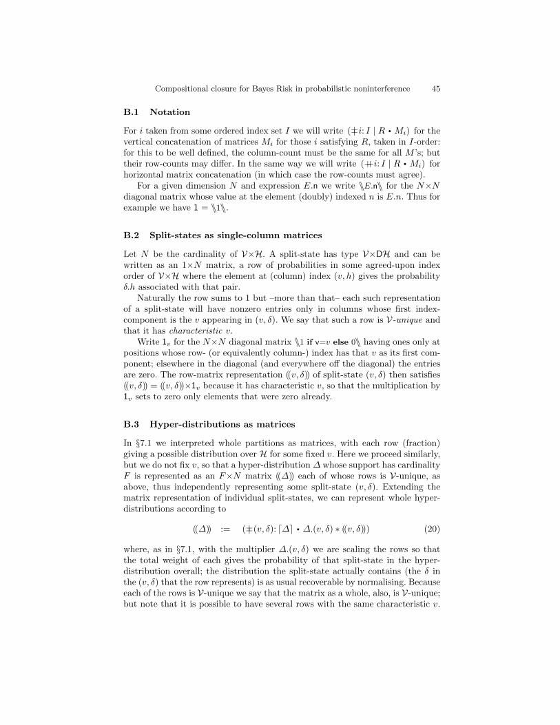
Compositional closure for Bayes Risk in probabilistic noninterference 45
B.1 Notation
For i taken from some ordered index set I we will write (++i: I | R ·Mi) for thevertical concatenation of matrices Mi for those i satisfying R, taken in I-order:for this to be well defined, the column-count must be the same for all M ’s; buttheir row-counts may differ. In the same way we will write (++i: I | R ·Mi) forhorizontal matrix concatenation (in which case the row-counts must agree).
For a given dimension N and expression E.n we write \\E.n\\ for the N×Ndiagonal matrix whose value at the element (doubly) indexed n is E.n. Thus forexample we have 1 = \\1\\.
B.2 Split-states as single-column matrices
Let N be the cardinality of V×H. A split-state has type V×DH and can bewritten as an 1×N matrix, a row of probabilities in some agreed-upon indexorder of V×H where the element at (column) index (v, h) gives the probabilityδ.h associated with that pair.
Naturally the row sums to 1 but –more than that– each such representationof a split-state will have nonzero entries only in columns whose first index-component is the v appearing in (v, δ). We say that such a row is V-unique andthat it has characteristic v.
Write 1v for the N×N diagonal matrix \\1 if v=v else 0\\ having ones only atpositions whose row- (or equivalently column-) index has that v as its first com-ponent; elsewhere in the diagonal (and everywhere off the diagonal) the entriesare zero. The row-matrix representation ((v, δ)) of split-state (v, δ) then satisfies((v, δ)) = ((v, δ))×1v because it has characteristic v, so that the multiplication by1v sets to zero only elements that were zero already.
B.3 Hyper-distributions as matrices
In §7.1 we interpreted whole partitions as matrices, with each row (fraction)giving a possible distribution over H for some fixed v. Here we proceed similarly,but we do not fix v, so that a hyper-distribution ∆ whose support has cardinalityF is represented as an F×N matrix ((∆)) each of whose rows is V-unique, asabove, thus independently representing some split-state (v, δ). Extending thematrix representation of individual split-states, we can represent whole hyper-distributions according to
((∆)) := (++(v, δ): d∆e · ∆.(v, δ) ∗ ((v, δ))) (20)
where, as in §7.1, with the multiplier ∆.(v, δ) we are scaling the rows so thatthe total weight of each gives the probability of that split-state in the hyper-distribution overall; the distribution the split-state actually contains (the δ inthe (v, δ) that the row represents) is as usual recoverable by normalising. Becauseeach of the rows is V-unique we say that the matrix as a whole, also, is V-unique;but note that it is possible to have several rows with the same characteristic v.

46 Annabelle McIver, Larissa Meinicke, and Carroll Morgan
V-uniqueness means that no two distinct v’s appear with non-zero probabilityin the same row.
As for partitions, in such matrices we define similarity between rows andsay that a hyper-distribution is in reduced matrix representation if all its similarrows have been added together, and all its all-zero rows have been removed. Wesay that two hyper-distribution matrices are similar (≈) if their reductions areequivalent up to a reordering of rows. Similarity is a congruence for matrix mul-tiplication on the right, but not on the left; vertical concatenation (++) respectssimilarity on both sides.
While the column-order of ((∆)) is fixed by our (arbitrary) ordering of V×H,the row-order might vary since there is no intrinsic order on fractions. We there-fore regard ((∆)) as determined only up to similarity, and our reasoning belowwill be restricted to operations for which similarity is a congruence. In partic-ular we have that ((∆1))≈((∆2)) implies ∆1=∆2, i.e. that ((·)) is injective up tosimilarity.
The operation ((·)) on (sub-)hyper-distributions is linear in the sense that
((p∗∆)) = p ∗ ((∆))and ((∆1+∆2)) ≈ ((∆1)) ++ ((∆2)) .
(21)
B.4 Classical commands as matrices
We recall from §2.3 that the classical “relational” semantics [[P ]]C of a programP is a function V×H→D(V×H) and may hence be treated (just as D.v.h from§7.1 was) as an N×N matrix written (|P |) whose value in row (v, h) and column(v′, h′) is just [[P ]]C .(v, h).(v′, h′). 30
Sequential composition between classical commands is then represented bymatrix multiplication, in the usual Markov style, so that we have
(|P1;P2|) = (|P1|)× (|P2|) . (22)
B.5 Secure commands as matrices
We will establish that for any secure program P there is an I-indexed set ofN×N matrices such that
(( [[P ]].(v, δ) )) ≈ (++i: I · ((v, δ))×Mi) (23)
for any split-state (v, δ). We think of the matrices as giving a normal form forP . Using the normal form, we will be able to represent the lifting of P ’s securesemantics using matrix operations, since then
(( (� (v, δ):∆ · [[P ]].(v, δ)) )) ≈ (++i: I · ((∆))×Mi) (24)
can be established by the calculation
30 Note that operation (|·|) applies to texts, i.e. syntax but ((·)) applies to hyper-distributions, i.e. semantics.

Compositional closure for Bayes Risk in probabilistic noninterference 47
(( (� (v, δ):∆ · [[P ]].(v, δ)) ))= (( (
∑(v, δ): d∆e · ∆.(v, δ) ∗ [[P ]].(v, δ) ) )) “definition expected value §2.1”
≈ (++(v, δ): d∆e · ∆.(v, δ) ∗ (([[P ]].(v, δ)))) “from (21)”
≈ (++(v, δ): d∆e · ∆.(v, δ) ∗ (++i: I · ((v, δ))×Mi) ) “normal form (23)”
= (++(v, δ): d∆e; i: I · (∆.(v, δ) ∗ ((v, δ)))×Mi) “distribute multiplication”
≈ (++i: I · (++(v, δ): d∆e · ∆.(v, δ) ∗ ((v, δ))) ×Mi) “rearrange rows; distributepost-multiplication”
≈ (++i: I · ((∆))×Mi) . “from (20) defining ((∆))”
We now show by structural induction how embedded classical commands, generalchoice, sequential composition (and hence all of our secure commands) can betranslated into this normal form.
Embedded classical commands In Def. 3 from §8.1 we gave the semantics[[〈〈P 〉〉]] of a program P considered as an atomic unit; we now do the same herein matrix style.
If we were to execute an atomic program 〈〈P 〉〉 from a split-state (v, δ), in thematrix style we would begin by calculating ((v, δ))×(|P |), giving again a singlerow; but that row might not be V-unique, in which case a further step wouldbe needed. We’d split its possibly non-unique rows into (maximally) V-uniqueportions, an operation that corresponds roughly to the embed funtion used inDef. 1.
Given a row matrix R that is V×H-indexed by column (such as the out-put ((v, δ))×(|P |) from just above) the splitting of its possibly non-unique row isachieved via
embed.R := (++v′:V · R× 1v′) , (25)
in which each of the values v′ in V is used, in turn, to construct a row ma-trix of characteristic v′ projected from R by zeroing all other entries: thosecharacteristic-v′ projections are then stacked on top of each other with (++) tomake a single (possibly quite tall!) matrix that is derived from R but now isV-unique. 31 With that apparatus, we have
(( [[〈〈P 〉〉.(v, δ)]] )) ≈ (++v′:V · ((v, δ))× (|P |)× 1v′) , (26)
thereby giving the V-unique matrix representation (up to similarity) of thehyper-distribution output by 〈〈P 〉〉 if executed from incoming split-state (v, δ). 32
General choice For both general choice and sequential composition we assumeinductively that the semantics of subprograms P1 and P2 can be written in
31 For example, if the row R is V-unique already then R′:= embed.R will stack up agreat many all-zero rows. But still we will have R≈R′, so no damage is done.
32 Note the algebra of similarity here: if we have R≈((v, δ)) for some R, then(++v
′:V · R× (|P |)× 1v′) is similar to the right-hand side above.

48 Annabelle McIver, Larissa Meinicke, and Carroll Morgan
matrix normal form so that for each split-state (v, δ) we have
(( [[Pi]].(v, δ) )) ≈ (++ji: Ji · ((v, δ))×Mi,ji) .
To show that general choice can be expressed in matrix normal form, we usethe following identity which expresses the conditioning of a split-state (v, δ) byexpression E.v.h in terms of matrix operations:
(�h: δ · E.v.h) ∗ ((v, {{h: δ | E.v.h}})) = ((v, δ))× \\E.v.h\\ . (27)
We then have
(( [[P1 q.v.h⊕ P2]].(v, δ) ))
=(( p ∗ [[P1]].(v, {{h: δ | q.v.h}}) + (1−p) ∗ [[P2]].(v, {{h: δ | 1−q.v.h}}) ))
“general choice from Fig. 1; p:= (�h: δ · q.v.h)”
≈p ∗ (( [[P1]].(v, {{h: δ | q.v.h}}) )) ++ (1−p) ∗ (( [[P2]].(v, {{h: δ | 1−q.v.h}}) ))
“from (21)”
≈p ∗ (++j1: J1 · ((v, {{h: δ | q.v.h}}))×M1,j1)
++ (1−p) ∗ (++j2: J2 · ((v, {{h: δ | 1−q.v.h}}))×M2,j2)
“inductive assumption: matrix normal form of P1 and P2”
=(++j1: J1 · (p ∗ ((v, {{h: δ | q.v.h}})))×M1,j1)
++ (++j2: J2 · ((1−p) ∗ ((v, {{h: δ | 1−q.v.h}})))×M2,j2)
“distribute scalar multiplications”
=(++j1: J1 · ((v, δ))× \\q.v.h\\ ×M1,j1)
++ (++j2: J2 · ((v, δ))× \\1−q.v.h\\ ×M2,j2)
“recall p:= (�h: δ · q.v.h); from (27)”
=(++i: {1, 2}; j: Ji · ((v, δ))× \\pi.v.h\\ ×Mi,j) .
“Let p1.v.h:= q.v.h and p2.v.h:= 1−q.v.h”
Sequential composition For sequential composition of P1 and P2 we have
(( [[P1;P2]].(v, δ) ))
=((
(� (v′, δ′): [[P1]].(v, δ) · [[P2]].(v′, δ′))))
“Composition from Fig. 1”
≈ (++j2: J2 · (([[P1]].(v, δ)))×M2,j2) “(24); matrix normal form of P2”
≈ (++j1: J1; j2: J2 · ((v, δ))×M1,j1 ×M2,j2) . “matrix normal form of P1”
B.6 Refinement as matrix multiplication
In §7.1 we showed how refinement between partitions could be defined usingmatrix multiplication. We can promote this to hyper-distributions by dealing
Compositional closure for Bayes Risk in probabilistic noninterference 49
with each v separately: we have that hyper-distribution ∆S is refined by ∆I justwhen for each v∈V there exists a refinement matrix (i.e. a non-negative, columnone-summing matrix) Rv such that
Rv × ((∆S))× 1v ≈ ((∆I))× 1v . (28)
The effect of requiring similarity for each v separately is to prevent rows withdiffering v’s from being added together.
C Proofs for the refinement relation
C.1 Secure programs are partially ordered by (v)
We show (Thm. 1 in §6.5) that the refinement relation (v) defines a partial orderover hyper-distributions. It follows by extension that it is a partial order oversecure programs.
Reflexivity For any hyper-distribution ∆ reflexivity holds trivially since, foreach v, the intermediate partition fracs.∆.v is both similar to and as fine as itself.
Transitivity Assume that ∆1v∆2 and ∆2v∆3. It is enough to show that foreach v we have fracs.∆1.v v fracs.∆3.v. For each i let Πi be the N×N matrixrepresentation (§7.1) of fracs.∆i.v for some N . To prove Π1vΠ3, we need to finda refinement matrix R31 such that Π3 is R31×Π1.
From above there are refinement matrices R32, R21 with Π3 = R32×Π2 andΠ2 = R21×Π1. Thus R31 defined R32×R21 satisfies Π3 = R31×Π1, and it is arefinement matrix by Property (11) from §7.1.
Antisymmetry Assume that both ∆1v∆2 and ∆2v∆1 but ∆1 6= ∆2. Fromthe first and third assumptions, with Lem. 6 (§G.1) we have that the ShannonEntropy of ∆1 is strictly less than that of ∆2; from the second and third, wehave the opposite — thus a contradiction.
C.2 Monotonicity of secure programs w.r.t. (v)
We use the following technical results to verify that (v) is monotonic with respectto secure program contexts (Thm. 2 from §6.5). They are verified using thematrix algebra from §B above.
Lemma 3. For any indexed set of matrices {i: I · Mi} each of dimensionF×N and corresponding refinement matrices Ri each having Fi rows and Fcolumns, there exists a refinement matrix R such that
(++i: I · Ri ×Mi) = R× (++i: I ·Mi) . (29)

50 Annabelle McIver, Larissa Meinicke, and Carroll Morgan
Proof: Refinement matrix R can be given directly as
(++i: I · (++ i′: I · ( Ri if i = i′ else 0Fi×F )) ) .
That R is a refinement matrix (i.e. it has non-negative entries and is column-one-summing) follows from its definition and the fact that each Ri is a refinementmatrix. It can be established by matrix multiplication that (29) holds. 33 2
Lemma 4. Additive monotonicity of hyper-distributions For probability p: [0, 1],and hyper-distributions ∆S1 , ∆S2 , ∆I1 , ∆I2 we have that ∆Si v ∆Ii implies
∆S1 p⊕∆S2 v ∆I1 p⊕∆I2 .
Proof: From (28) it is enough for each v to find a refinement matrix R suchthat
R× ((∆S1 p⊕∆S2))× 1v ≈ ((∆I1 p⊕∆I2))× 1v .
We have:
((∆I1 p⊕∆I2 ))× 1v≈ ( p∗((∆I1)) ++ (1−p)∗((∆I2)) )× 1v “from (21)”
= p∗((∆I1))× 1v ++ (1−p)∗((∆I2))× 1v “distribute post-multiplication”
≈p ∗R1 × ((∆S1
))× 1v ++ (1−p) ∗R2 × ((∆S2))× 1v
“∆Siv∆Ii implies ((∆Ii))×1v ≈ Ri×((∆Si))×1v for some refinementmatrix Ri”
=(R1 × p∗((∆S1)) ++ R2 × (1−p)∗((∆S2)) )× 1v
“commute scalar multiplication; distribute post-multiplication”
=R× ( p ∗ ((∆S1
)) ++ (1−p) ∗ ((∆S2)) )× 1v
“Lem. 3 for some refinement matrix R”
≈ R× ((∆S1 p⊕∆S2))× 1v . “from (21)”
2
Lemma 5. Pointwise monotonicity For all program texts P and hyper-distribut-ions ∆S and ∆I such that ∆S v ∆I , we have
(� (v, δ):∆S · [[P ]].(v, δ)) v (� (v, δ):∆I · [[P ]].(v, δ)) .
Proof: Let {i: I · Mi} be a set of N×N matrices giving the normal formfor [[P ]] as at (23) above, so that for any (v, δ) we have
(( [[P ]].(v, δ) )) ≈ (++i: I · ((v, δ))×Mi) .
From (28) and (24), it is enough to show that for each v′∈V there exists a refine-ment matrixR such thatR× (++i: I · ((∆S))×Mi)×1v′ ≈ (++i: I ·Mi×((∆I)))×1v′ .We have
33 A sketch of the block matrices helps to see the pattern.
Compositional closure for Bayes Risk in probabilistic noninterference 51
(++i: I · ((∆I))×Mi) × 1v′
≈ (++i: I · (++v:V · ((∆I))× 1v) ×Mi) × 1v′ “((∆I)) is V-unique”
= (++i: I; v:V · ((∆I))× 1v ×Mi) × 1v′ “distribute post-multiplication”
≈(++i: I; v:V · Rv × ((∆S))× 1v ×Mi) × 1v′
“∆S v ∆I implies ((∆I))× 1v ≈ Rv × ((∆S))× 1v for somerefinement matrix Rv”
= R× (++i: I; v:V · ((∆S))× 1v ×Mi) × 1v′ “Lem. 3for some refinement matrix R”
≈ R× (++i: I · ((∆S))×Mi) × 1v′ . “distribute post-multiplication;((∆S)) is V-unique”
2
Monotonicity of secure programs w.r.t. (v) Using Lem. 4 and Lem. 5 wenow prove Thm. 2 from §6.5. We must show that if SvI then C(S)vC(I) for allcontexts C built from programs as defined in Fig. 1.
We use structural induction. For the base case, context C(S):=S is triviallymonotonic.
General probabilistic choice (and hence probabilistic and conditional choice)is trivially monotonic in either argument from monotonicity of addition overhyper-distributions (Lem. 4). For example, for monotonicity in the first argumentwe have
[[S q.v.h⊕R]].(v, δ)=
([[S]].(v, {{h: δ | q.v.h}}) qδ⊕ [[R]].(v, {{h: δ | 1−q.v.h}}))“Let qδ:= (�h: δ · q.v.h); General choice from Fig. 1”
v ([[I]].(v, {{h: δ | q.v.h}}) qδ⊕ [[R]].(v, {{h: δ | 1−q.v.h}})) “S v I; Lem. 4”
= [[I q.v.h⊕R]].(v, δ) . “General choice from Fig. 1”
To show monotonicity of sequential composition in its right-hand argumentwe have for any programs R and S v I and initial state (v, δ) that
[[R;S]].(v, δ)= (� (v′, δ′): [[R]].(v, δ) · [[S]].(v′, δ′)) “Composition from Fig. 1”
v (� (v′, δ′): [[R]].(v, δ) · [[I]].(v′, δ′)) “S v I; Lem. 4”
= [[R; I]].(v, δ) . “Composition from Fig. 1”
For monotonicity in the first argument we have
[[S;R]].(v, δ)= (� (v′, δ′): [[S]].(v, δ) · [[R]].(v′, δ′)) “Composition from Fig. 1”
v (� (v′, δ′): [[I]].(v, δ) · [[R]].(v′, δ′)) “S v I and Lem. 5”
= [[I;R]].(v, δ) . “Composition from Fig. 1”

52 Annabelle McIver, Larissa Meinicke, and Carroll Morgan
D Example of completeness construction
Here we illustrate the completeness proof set out in §7.3 by applying it to theexample of §6, where we claimed that P4 6vP2. We use §7.3 to find a C such thatindeed P4;C 6� P2;C.
Our v′ is 1, since that is where we find the difference between P2 and P4 inthe residual uncertainties of h; with that, we extract the fractions
when v′=1
{ΠP4 := 〈{{1@ 1
4 , 3@ 112 }}, {{1@ 1
12 , 3@ 14 }}〉
ΠP2:= 〈{{1@ 1
6 }}, {{1@ 16 , 3@ 1
6 }}, {{3@ 16 }}〉
and find that there are two values of h, two fractions in ΠP4 and three fractionsin ΠP2 . Accordingly we set N to 3 and include an extra column for h=2 andan extra, zero fraction in ΠP4
. Note that∑ΠP2
=∑ΠP4
and that the totalweight (of each) is 2/3.
The N×N matrix corresponding to ΠP2is then as at right
1/6 0 01/6 0 1/60 0 1/6
with its columns corresponding to values 1, 2, 3 of h and therows to ΠP2 ’s three fractions. The point obtained by con-catenating the rows is (1/6, 0, 0, 1/6, 0, 1/6, 0, 0, 1/6), and isin 9-dimensional space; but to avoid a proliferation of fractions, we scale ev-erything up from now on by a factor of 12, and so take xP2
to be the point(2, 0, 0, 2, 0, 2, 0, 0, 2).
Now the scaled-up (and extended) matrix corresponding to ΠP4 , with a se-lection of refinement-forming matrices M in MN , is given by3 0 1
1 0 30 0 0
and
1 1 10 0 00 0 0
,
1 0 10 1 00 0 0
,
1 0 10 0 00 1 0
,
0 1 11 0 00 0 0
· · ·Carrying out the matrix multiplications gives us these four possible refinementsof ΠP4
: 4 0 40 0 00 0 0
,
3 0 11 0 30 0 0
,
3 0 10 0 01 0 3
,
1 0 33 0 10 0 0
· · · .Doing all of them for M in MN , and concatenating their rows to make pointsin 9-dimensional space, gives us this collection of refinements altogether:
{ (4, 0, 4, 0, 0, 0, 0, 0, 0) , (3, 0, 1, 1, 0, 3, 0, 0, 0) , (3, 0, 1, 0, 0, 0, 1, 0, 3) ,(1, 0, 3, 3, 0, 1, 0, 0, 0) , (0, 0, 0, 4, 0, 4, 0, 0, 0) , (0, 0, 0, 3, 0, 1, 1, 0, 3) ,(1, 0, 3, 0, 0, 0, 3, 0, 1) , (0, 0, 0, 1, 0, 3, 3, 0, 1) , (0, 0, 0, 0, 0, 0, 4, 0, 4) } .
(30)
Our claim that P4 6vP2 suggests that the point xP2 (corresponding to the matrixderived from ΠP2
) should not lie in the convex closure of the points (30) above.We can see this easily by concentrating on the first and third dimensions
only: for Π2
we get (2, 0); and for ΠP4, that is (30), after removing duplicates
we get (4, 4), (3, 1), (1, 3) and (0, 0). The ΠP2-point xP2 is not in the convexclosure of the other four because all of them have their two coordinates bothpositive or both zero, a property preserved by any convex combination but notshared by (2, 0).

Compositional closure for Bayes Risk in probabilistic noninterference 53
dt
t
t
t
��������
��������
��������
��������
����
����
�����1
y = (x−1)/3
We insert a hyperplane (just a line, in2-space) midway between the separatedpoint and the convex shape, parallel to theboundary of the latter.
Fig. 4. Finding a separating hyperplaney = (x−1)/3 in 2-space.
Now that we can concentrate onjust two dimensions, it’s easy to find aseparating hyperplane with a picture.Fig. 4 shows the ΠP2-point as an opencircle at (2, 0), while the filled cir-cles give the vertices of the diamond-shaped convex closure correspondingto refinements ofΠP4
. Clearly the (de-generate) hyperplane y = (x−1)/3separates the point from the diamond.The normal of that hyperplane (upand left, perpendicular to the line)has direction (−1, 3), and when wefill in the other seven dimensions aszero –since they’re not needed forseparation– that gives us a candidatenormal of X:= (−1, 0, 3, 0, 0, 0, 0, 0, 0)in 9-space. By translating X to ma-trix form and transposing it, we can
then give a tentatitive definition of D as shown at right. However this is notquite our final value for it. −1 0 0
0 0 03 0 0
The dot-product of X with ΠP2, that is tr.(ΠP2
×D),turns out to be −2; and with the refinements of ΠP4
shownat (30) we get the dot-products 8 and 0 (multiple times),showing indeed the separation we expect, but in the wrong direction: the values0 and 8 for P4 are both strictly greater than the value −2 for P2, and we wantthem to be strictly less. Accordingly we multiply the tentative D above by −1 34
and then add 3 to all its elements to make them non-negative; finally we divideeverything by 10 to make its rows sum to no more than 1. To get the final D fromthis we must then add a new “zero-th column” to make each row one-summingexactly. That gives
D :=
↓ Zero’th column, for one-summing
0 0.4 0.3 0.30.1 0.3 0.3 0.30.4 0 0.3 0.3
.
The distinguishing context (− ; C), say, must then overwrite h according to the
distribution given by a row of D, the one selected by the value h of h incomingto C; thus we construct C to be
if v=1 then h:∈ ({{1@ 0.4, 2@ 0.3, 3@ 0.3}} if h=1 else {{0@ 0.4, 2@ 0.3, 3@ 0.3}})else h:= 0 fi ,
34 The fact we can simply multiply by −1 to reverse the sense of the comparison doesnot mean we can just as easily construct a context to show P2 6vP4 — which wouldindeed be a worry. In fact for P2 6vP4 we’d need a shape XP2 and a point xP4 ; andthen we would find xP4 inside the shape XP2 , thus unable to be separated from it.
54 Annabelle McIver, Larissa Meinicke, and Carroll Morgan
with the outer if effectively restricting our attack to occur only when v′=1.(That allows us to ignore the h=2 case in D, as well.) Thus we have our context(− ; C). Let us now check that it actually works.
We begin with P4;C. Its output hyper-distribution is (after some calculation)given by
{{ (0, {{0}})@ 13 ,
(1, {{0@ 0.1, 1@ 0.3, 2@ 0.3, 3@ 0.3}})@ 13 ,
(1, {{0@ 0.3, 1@ 0.1, 2@ 0.3, 3@ 0.3}})@ 13 }} ,
whose Bayes Vulnerability is 1/3∗1 + 1/3∗0.3 + 1/3∗0.3 ≈ 0.53. On the otherhand, for P2;C the output hyper-distribution is
{{ (0, {{0}})@ 13 ,
(1, {{1@ 0.4, 2@ 0.3, 3@ 0.3}})@ 16 ,
(1, {{0@ 0.2, 1@ 0.2, 2@ 0.3, 3@ 0.3}})@ 13 ,
(1, {{0@ 0.4, 2@ 0.3, 3@ 0.3}})@ 16 }} ,
and here the vulnerability is 1/3∗1 + 1/6∗0.4 + 1/3∗0.3 + 1/6∗0.3 ≈ 0.55. Notethat in the third summand we took 0.3 rather than the larger 0.4 associatedwith 0, since as part of our construction we exclude guesses that h is 0. 35
Thus we have established that P4;C 6� P2;C (for the adjusted C — seeFootnote 35), because the vulnerability of the former is 0.53 but for the latterthe vulnerability is the greater 0.55. Hence when our refinement relation insiststhat P4 6vP2 –as we argued earlier above– in fact it is not being too severe, butrather it is acting just as a compositional closure should. It protects us not onlyagainst the context C we just made, but all other contexts too — in spite of thefact that in isolation P4 and P2 are not distinguished by elementary testing.
Finally, in this example there are many hyperplanes with distinct normalsthat achieve the separation we need, and each of these may be used to constructdifferent distinguishing contexts. For example, since there exists a separatinghyperplane with normal (0, 0, 2, 1, 0, 0, 1, 0, 0) we can use it to define another
35 Dealing with this detail would split the 0-case in half, uniformly distributed over−1,−2, since the resulting probability 0.4/2 for each would then be small enoughthat a Bayes-Vulnerability attack would never choose it. The adjusted context C′
would contain
h:∈ ({{[email protected], [email protected], [email protected]}} if h=1 else {{ − [email protected],−[email protected], [email protected], [email protected]}})
and the resulting output for P2;C′ would be
{{ (0, {{0}})@13 ,
(1, {{[email protected], [email protected], [email protected]}})@16 ,
(1, {{ − [email protected],−[email protected], [email protected], [email protected], [email protected]}})@13 ,
(1, {{ − [email protected],−[email protected], [email protected], [email protected]}})@16 }} ,
in which neither −2 nor −1 would ever be chosen for a Bayes-Vulnerability attack.
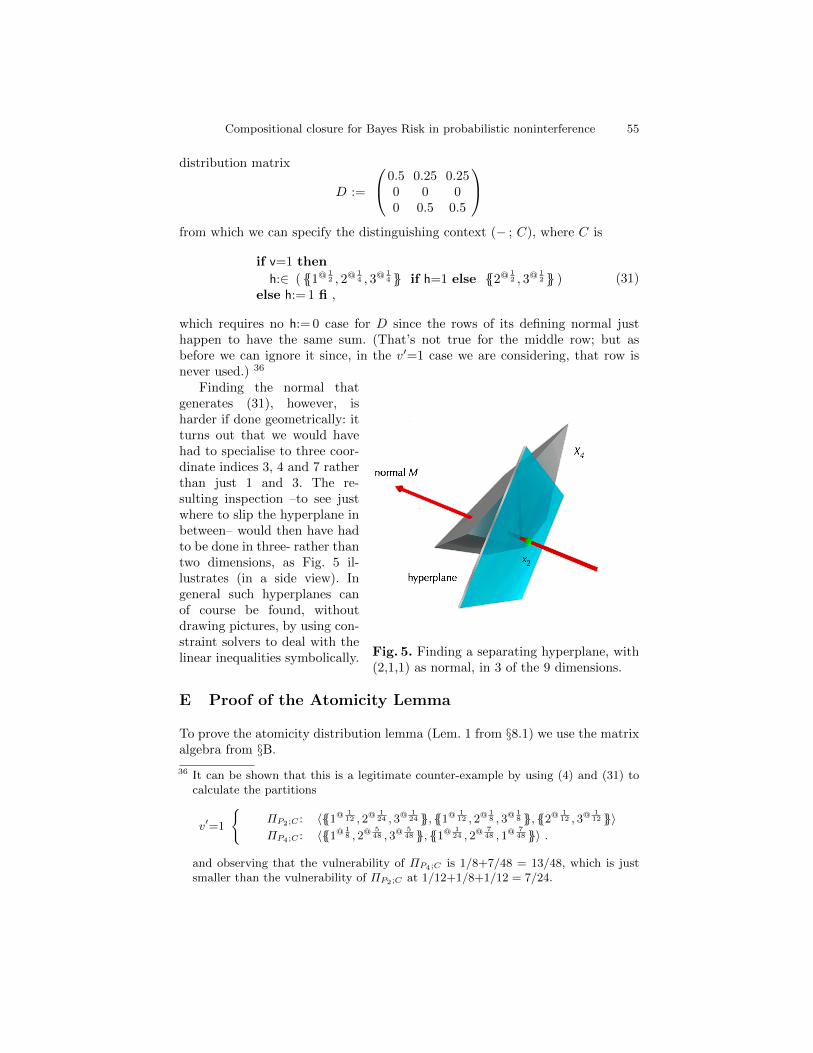
Compositional closure for Bayes Risk in probabilistic noninterference 55
distribution matrix
D :=
0.5 0.25 0.250 0 00 0.5 0.5
from which we can specify the distinguishing context (− ; C), where C is
if v=1 then
h:∈ ( {{1@ 12 , 2@ 1
4 , 3@ 14 }} if h=1 else {{2@ 1
2 , 3@ 12 }} )
else h:= 1 fi ,(31)
which requires no h:= 0 case for D since the rows of its defining normal justhappen to have the same sum. (That’s not true for the middle row; but asbefore we can ignore it since, in the v′=1 case we are considering, that row isnever used.) 36
Fig. 5. Finding a separating hyperplane, with(2,1,1) as normal, in 3 of the 9 dimensions.
Finding the normal thatgenerates (31), however, isharder if done geometrically: itturns out that we would havehad to specialise to three coor-dinate indices 3, 4 and 7 ratherthan just 1 and 3. The re-sulting inspection –to see justwhere to slip the hyperplane inbetween– would then have hadto be done in three- rather thantwo dimensions, as Fig. 5 il-lustrates (in a side view). Ingeneral such hyperplanes canof course be found, withoutdrawing pictures, by using con-straint solvers to deal with thelinear inequalities symbolically.
E Proof of the Atomicity Lemma
To prove the atomicity distribution lemma (Lem. 1 from §8.1) we use the matrixalgebra from §B.
36 It can be shown that this is a legitimate counter-example by using (4) and (31) tocalculate the partitions
v′=1
{ΠP2;C : 〈{{1@ 1
12 , 2@ 124 , 3@ 1
24 }}, {{1@ 112 , 2@ 1
8 , 3@ 18 }}, {{2@ 1
12 , 3@ 112 }}〉
ΠP4;C : 〈{{1@ 18 , 2@ 5
48 , 3@ 548 }}, {{1@ 1
24 , 2@ 748 , 1@ 7
48 }}〉 .
and observing that the vulnerability of ΠP4;C is 1/8+7/48 = 13/48, which is justsmaller than the vulnerability of ΠP2;C at 1/12+1/8+1/12 = 7/24.

56 Annabelle McIver, Larissa Meinicke, and Carroll Morgan
Suppose we have matrix representations (|P{1,2}|) for the classical programtexts P1 and P2 and a row-matrix representation ((v, δ)) of an incoming split-state.
If from every initial and final v-state of P1;P2 it is possible to determine theintermediate value of v (after P1 and before P2) then there must exist a totalfunction f :V→V→V such that for all v, v′ we have
1v × (|P1|)× (|P2|)× 1v′ = 1v × (|P1|)× 1f.v.v′ × (|P2|)× 1v′ (32)
from which we have for all v 6= f.v.v′ that
1v × (|P1|)× 1v × (|P2|)× 1v′ = 0N , (33)
where 0N is the N×N matrix of zeros.
Assuming such an f with properties (32) and (33), we can calculate
(([[〈〈P1;P2〉〉]].(v, δ)
))≈ (++v
′:V · ((v, δ))× (|P1;P2|)× 1v′) “embedding”
= (++v′:V · ((v, δ))× (|P1|)× (|P2|)× 1v′) “classical composition”
= (++v′:V · ((v, δ))× 1v × (|P1|)× (|P2|)× 1v′) “((v, δ))×1v = ((v, δ))”
= (++v′:V · ((v, δ))× 1v × (|P1|)× 1f.v.v′ × (|P2|)× 1v′) “(32)”
= (++v′, v:V | v=f.v.v′ · ((v, δ))× 1v × (|P1|)× 1v × (|P2|)× 1v′) “one-point rule
for (++)”
≈(++v
′, v:V | v=f.v.v′ · ((v, δ))× 1v × (|P1|)× 1v × (|P2|)× 1v′)
++ (++v′, v:V | v 6=f.v.v′ · 01×N )
“01×N is unit of concatenation, up to similarity”
=(++v
′, v:V | v=f.v.v′ · ((v, δ))× 1v × (|P1|)× 1v × (|P2|)× 1v′)
++ (++v′, v:V | v 6=f.v.v′ · ((v, δ))× 1v × (|P1|)× 1v × (|P2|)× 1v′)
“01×N = ((v, δ))×0N , (33)”
≈
(++v′, v:V · ((v, δ))× 1v × (|P1|)× 1v × (|P2|)× 1v′)
“v=f.v.v′ and v 6=f.v.v′ are disjoint and exhaustive;(++) is commutative and associative up to similarity”
= (++v′, v:V · ((v, δ))× (|P1|)× 1v × (|P2|)× 1v′) “((v, δ))×1v = ((v, δ))”
= (++v′:V · (++v · ((v, δ))× (|P1|)× 1v) × (|P2|)× 1v′) “distribute ++”
≈((
[[〈〈P1〉〉; 〈〈P2〉〉]].(v, δ))), “composition, embedding”
whence our result follows because ((·)) is injective up to similarity and (v, δ) wasarbitrary.

Compositional closure for Bayes Risk in probabilistic noninterference 57
F Informal description of the Oblivious Transferimplementation 37
Given are two agents B,C; Agent B has two messsages m{0,1}, bit-strings of thesame length; Agent C has a message variable m and a choice c: {0, 1} of whichof m{0,1} is to be assigned to m. The specification is thus
visB m0,m1; visC m, c;m:=mc .
Note that B does not discover c and that C does not discover m¬c.
The implementation is, informally, as follows:
This is the prelude of the protocol1. Agent B chooses privately two random bit-strings m′{0,1} to be used for ∇-
encrypting m{0,1} respectively.2. Agent C chooses privately in c′: {0, 1} which of the encrypting strings m′{0,1}
will be revealed to her.3. A trusted third party collects both m′{0,1} from B, collects c′ from C and
then reveals (only) m′c′ to C. She throws m′¬c′ away, and then leaves.
From here is the main part of the protocol4. Agent C then tells B to encrypt and send messages in the following way:
(a) If Agent C wants m0 and has m′0, then she instructs B to send herboth m0∇m′0 and m1∇m′1. Because she has m′0 she can recover m0 via(m0∇m′0)∇m′0; but she cannot recover m1.
(b) Similarly, if Agent C wants m0 but has m′1 instead (of m′0), then shesimply instructs B to send her both m0∇m′1 and m1∇m′0, i.e. with theencryption the other way around.
(c) If Agent C wants m1 and has m′0 — as for (4b).(d) If Agent C wants m1 and has m′1 — as for (4a).The four cases (4a–4d) can be described succinctly –if cryptically– simplyby instructing B to send mi∇m′i∇c∇c′ for i = 0, 1.
37 An even more informal description is this fairy tale. An Apprentice magician is aboutto graduate, and he must now choose between black- or white magic. His Sorcererwill allow him to read either the Black Tome or the White Tome, not both; and hischoice must be his own, uncoerced, thus never revealed to the Academy.
The Sorcerer summons a trusted third party Djinn who gives him two locks, oneblack and one white; and the Djinn gives a single, golden key to the Apprentice.On the key is a small dot that only the Apprentice can see: it is the colour of thematching lock. The Djinn then returns to his own dimension.
The Apprentice tells the Sorcerer to match the lock colours to the Tomes, or toreverse them: it depends on whether his choice matches the colour of the dot. TheSorcerer then leaves; the Apprentice can unlock only the Tome of his choice; and–provided he locks it again– no one afterwards will know which one he read.

58 Annabelle McIver, Larissa Meinicke, and Carroll Morgan
Note that only Step (3) involves private messages (first between B and the thirdparty, and then between the third party and C), and that is only in the prelude,before any of the actual data m{0,1}, c has appeared. Steps (1) and (2) involve nomessages at all; and the messages occurring in Step (4) are ∇-encrypted already.In effect the prelude has created a one-time pad.
A formal derivation of this implementation is given elsewhere [27].
G Alternative uncertainty measures
G.1 Shannon Entropy
The Shannon Entropy of a (full) distribution δ:DX is H.δ:= (� d: δ · − lg(δ.d)),that is the weighted average of the negated base-2 logarithms of its constituentprobabilities [33]. By extension, for any hyper-distribution ∆ we define the con-ditional Shannon Entropy H.∆ to be (� (v, δ):∆ · H.δ), the expected value ofthe entropies of its support [3].
Going further, if we split up our hyper-distribution by v into its partitions,we have an equivalent presentation of entropy as the sum of individual partition-entropies H.∆ = (
∑v:V · H.(fracs.∆.v)) , provided we define the entropy of a
single partition, and of a single fraction, as follows:
H.Π := (∑π:Π · H.π)
H.π := (� d:π · lg([π].d)) ,(34)
where we write lg for −lg to avoid a proliferation of minus signs, and [π] isnormalisation of the fraction π, scaling it up (if necessary) to give a distributionagain.
The ordering (�H) based on hyper-distributions
∆S �H ∆I := (ft.∆S = ft.∆I) ∧ (H.∆S ≤ H.∆I)
is then specified, as for the Bayes order (�), so that ∆S�H∆I if they are func-tionally equivalent and the uncertainty (the Shannon Entropy in this case) of ∆I
is no less than that of ∆S . It extends pointwise to secure programs. Furthermorewe write that S ≺H I when S �H I but I 6�H S.
Non-compositionality Consider again two functionally-equivalent programsfrom our three-box puzzle example from §2 and §4:
S := h:= 0⊕1⊕2; v:∈{{w@ h2 , b@1− h
2 }}; v:=⊥I2 := h:= 0⊕1⊕2; v:∈{{w@(h÷2), b@1−(h÷2)}}; v:=⊥
with final hyper-distributions
{{ (⊥, {{1@ 13 , 2@ 2
3 }}), (⊥, {{0@ 23 , 1@ 1
3 }}) }} (∆′S)
and {{ (⊥, {{2}})@ 13 , (⊥, {{0, 1}})@ 2
3 }} .. (∆′I2)
Compositional closure for Bayes Risk in probabilistic noninterference 59
The Shannon entropy of ∆′S , calculated 2 ∗ 12 ( 1
3 lg 13 + 2
3 lg 23 ), is slightly more
than 0.918, exceeding the entropy ∆′I2 that, by the simpler calculation given by13 (lg 1) + 2
3 (2∗ 12 lg 1
2 ), turns out to be exactly 23 ; and so I2�HS.
However if we define context C to be (− ; h:= (1 if h=2 else h)) then theentropy of C(I2) is the same as before at 2
3 ; but the entropy of C(S) is now onlya half of what it was, at ≈0.459. Hence C(I2) 6�H C(S).
Soundness We follow initially the structure of the soundness proof for BayesRisk. Fix an initial split-state and construct the output hyper-distributions∆′{S,I} that result from S, I respectively. Then since we assume SvI we must
have ∆′Sv∆′I . We now show that this implies ∆′S�H∆′I .
Since SvI trivially guarantees that ft.∆′S=ft.∆′I , we need to show that theShannon Entropy condition in (�H) is satisfied. Since we have that H.∆′ is(∑v′:V · H.(fracs.∆.v′)) , it is enough to show that for each v′:V the entropy of
Π ′S := fracs.∆′S .v′ is no less than the entropy of Π ′I := fracs.∆′I .v
′, provided thatΠ ′S ≈ Π ′ @∼ Π
′I for some partition Π ′ depending on v′.
For Π ′S≈Π ′ we consider the unique Π that is the reduction of both: it isformed in each case by adding together groups of similar fractions. From (34)and arithmetic, we obtain immediately that H.Π ′S = H.Π = H.Π ′. 38
For Π ′@∼Π′I we know that the fractions of Π ′I are sums of groups of not-
necessarily-similar fractions in Π ′. We consider the special case of just two frac-tions π{1,2} in Π ′ summing to a single fraction π:=π1+π2 in Π ′I , and look attheir relative contributions to the sum (34); we have
H.π= H.(π1+π2)
= (� d: (π1+π2) · lg([π1+π2].d))
= (� d:π1 · lg([π1+π2].d)) + (� d:π2 · lg([π1+π2].d))
† ≥ (� d:π1 · lg([π1].d)) + (� d:π2 · lg([π2].d)) “see below”
= H.π1 + H.π2 ,
that is that the contribution to the conditional entropy of π on its own is atleast as great as it was when was separated into π{1,2}.
For “see below” we refer to the Key Lemma [36, p5] which states that fortwo total distributions δ, δ′ of equal support, the weighted sum (� d: δ · lg(δ′.d))attains its minimum over δ′ when δ=δ′.
Extending the argument similarly to multiple additions gives H.Π ′ ≤ H.Π ′Ias required and thus we have H.Π ′S ≤ H.Π ′I overall. We note that the inequalityat † is strict when π1 6≈π2, because then e.g. [π1]6=[π1+π2]. 39 We have established
Theorem 6. Soundness of (v) w.r.t. (�H) For all secure programs S and Iand contexts C, we have that SvI implies C(S)�HC(I). 2
38 If π1≈π2 then [π1]=[π2]=[π1+π2] and so the line marked † below becomes an equality.39 This follows from a strengthening of the Key Lemma to “. . . only when δ=δ′,” which
is implied by the proof of Thm. 1 [op. cit.] immediately before.

60 Annabelle McIver, Larissa Meinicke, and Carroll Morgan
Finally, when SvI but S 6= I so that ∆′S 6=∆′I for some initial split-state wemust have Π ′S 6≈Π ′I for some final v′, since both those partitions are in reducedform: that is, reduced partitions cannot be similar without actually being equal.Thus also Π ′ 6≈Π ′I , and so we can find particular π1 6≈π2 to realise the strictinequality at †. That gives us
Lemma 6. Strict soundness For all hyper-distributions ∆{1,2} we have that∆1v∆2 but ∆1 6= ∆2 implies ∆1≺H∆2. 2
G.2 Marginal guesswork
The Marginal guesswork [30] of a distribution δ:DX is the least number ofguesses an attacker requires to be sure that her chance of guessing some h chosenaccording to δ is at least a given probability α. We define it
Wα.δ := (ui: 1..N | tiδ ≥ α)
where we write tiδ, or more generally tiπ for fraction π to mean the sum ofthe i greatest probabilities in π, and N is the cardinality of X . Note that bysuper-distribution of maximum over addition we have ti(π1+π2) ≤ tiπ1 +tiπ2
for any i in the proper range. To avoid clutter, we will omit the range 1..N fori from here on.
For a hyper-distribution ∆ we define
Wα.∆ := (ui | (� (v, δ):∆ · tiδ) ≥ α)or equivalently Wα.∆ := (ui | (
∑v:V;π: fracs.∆.v · tiπ) ≥ α)
(35)
which is the least value i such that if an attacker is allowed to make that manyguesses then she can discover the value of h with probability at least α.
Observe that our definition of Wα.∆ is not the same as the conditionalmarginal guesswork (� δ:∆ · Wα.δ) as conventionally defined [15]. We arguethat conditional marginal guesswork is not a reasonable measure of the numberof guesses required by an attacker to ensure that the probability of guessing hin ∆ is greater than α. Consider for example the hyper-distributions
∆S := {{(v, {{0}}), (v, {{1..4}})}} and ∆I := {{(v, {{0}} ⊕ {{1..4}})}} .40
Note that ∆Sv∆I since the latter is obtained by merging the two split-states ofthe former.
Now an attacker has more information about how h was chosen in ∆S than in∆I : for ∆S she knows not only that h is distributed according to the distribution{{0}} ⊕{{1..4}} overall (as for ∆I), but as well she knows when h was chosen from{{0}} and when h was chosen from {{1..4}}. However, when we set α:= 1/2 theconditional marginal guesswork of ∆S is 1
2 (1) + 12 (4α), that is 3/2 — which is
higher than for ∆I , which gives only 1. This suggests that it is harder for an
40 Alternatively we could write out {{0}} ⊕ {{1..4}} with its explicit probabilities as
{{0@ 12 , 1@ 1
8 , 2@ 18 , 3@ 1
8 , 4@ 18 }}, but we prefer to avoid the superscripts.

Compositional closure for Bayes Risk in probabilistic noninterference 61
attacker to guess h in ∆S than in ∆I , in spite of the fact that the attacker knowsmore about the final h-distribution in ∆S when launching an attack.
Using our Wα we have W1/2.∆S = W1/2.∆I , that is 1 in both cases: withjust one guess at her disposal an attacker is guaranteed to guess h at least halfthe time. Applying her one guess to ∆S , half the time she can guess 0 and issure to be right; in ∆1 she guesses 0 and will be right half the time.
The ordering between hyper-distributions based on marginal guesswork is
∆S �Wα∆I := (ft.∆S = ft.∆I) ∧ (Wα.∆S ≤Wα.∆I)
which extends pointwise to programs.
Non-compositionality When α is not zero, marginal guesswork –like the othermeasures– is non-compositional for our subset of programs. For such an α 6=0take, for example, functionally equivalent programs
S := h:∈{{0, 1, 2}} α⊕ {{−N..−1}};v:∈ ({{w@ h
2 , b@(1− h2 )}} if h≥0 else {{w@ 1
2 , b@12 }});
v:=⊥
I := h:∈{{0, 1, 2}} α⊕ {{−N..−1}};v:∈ ({{w@h÷2, b@1−h÷2}} if h≥0 else {{w@ 1
3 , b@23 }});
v:=⊥
such that if α=1 then N=0 else N ≥ 3× 1−αα . These programs have the final
output distributions
{{(⊥, {{1@ 13 , 2@ 2
3 }} α⊕ {{−N...−1}}), (⊥, {{0@ 23 , 1@ 1
3 }} α⊕ {{−N...−1}})}} (∆′S)
and {{(⊥, {{2}} α⊕ {{−N...−1}})@ 13 , (⊥, {{0, 1}} α⊕ {{−N...−1}})@ 2
3 }} . (∆′I)
We can calculate that both Wα.∆′S and Wα.∆
′I are 2, and so S �Wα
I, but thatfor context C defined as (− ; h:= (h ÷ 2 if h≥0 else h)) we have Wα.∆
′I is only
1, while Wα∆′S remains at 2 — and so C(S) 6�Wα C(I).
Soundness
Lemma 7. (v) implies (�Wα) For all hyper-distributions ∆S and ∆I and
probabilities α, if∆Sv∆I then also∆S�Wα∆I ; consequently SvI impliesS�WαI.Proof: From (35) and the definition of refinement (Def. 2, §6.4) it is enough
to show that for any partition Π and i in range that (i) if the fractions inΠ are similar then (
∑π:Π · tiπ) = ti (
∑π:Π) else (ii) (
∑π:Π · tiπ) ≥
ti (∑π:Π) . To show (ii) we have by generalising ti(π1+π2) ≤ tiπ1 +tiπ2 that
indeed(∑π:Π · tiπ) ≥ ti (
∑π:Π) ,
and for (i) we can replace inequality by equality since (ti) distributes oversummation in that case. 2

62 Annabelle McIver, Larissa Meinicke, and Carroll Morgan
Theorem 7. Soundness of (v) w.r.t. (�Wα) For all probabilities α, secure
programs S, I and contexts C we have that S v I implies C(S) �WαC(I).
Proof: Lem. 7 and monotonicity of (v) (Thm. 2 from §6.5). 2
G.3 Guessing entropy
The guessing entropy [19] of a distribution δ is the (least) average number ofguesses required to guess h in δ. It is equivalent to the average α-marginal guess-work over all values of α [30], and we define it
W.δ := (∑i: 1..N · uiδ) ,
where uiδ is the sum of the i smallest probabilities in δ. 41 Note that by subdis-tribution of minimum over addition we have ui(π1+π2) ≥ uiπ1 + uiπ2 for anyi in range. For hyper-distribution ∆ we define the conditional guessing entropy,thus
W.∆ := (� (v, δ):∆ ·W.δ)or equivalently W.∆ := (
∑v:V;π: fracs.∆.v ·W.π) ,
where W.π is defined in the same way as W.δ. We define the ordering by
∆S �W ∆I := (ft.∆S = ft.∆I) ∧ (W.∆S ≤W.∆I) ,
which extends pointwise to secure programs.
Non-compositionality To show non-compositionality of ordering (�W) werefer again (as we did for Shannon entropy in §G.1) to the functionally equivalentprograms S and I2. First we calculate that
W.∆′S = 2× 1
2 ( 13 + ( 1
3+ 23 )) = 4
3
and W.∆′I2
= 13 (1) + 2
3 ( 12 + ( 1
2+ 12 )) = 4
3 ,
so that we have I2 �W S. Again taking context C to be (− ; h:= (1 if h=2 else h))we get that the guessing entropy of C(S) is reduced to 7
6 while that of C(I2) isstill 4
3 , and hence C(I2) 6�W C(S).
Soundness
Lemma 8. (v) implies (�W) For all hyper-distributions ∆S and ∆I , we havethat ∆Sv∆I implies ∆S�W∆I ; and consequently SvI implies S�WI.
Proof: As in the proof of soundness for marginal guesswork, it is enoughto show that for any partition Π (i) if the fractions in Π are similar then(∑π:Π ·W.π) = W. (
∑π:Π) else (ii) (
∑π:Π ·W.π) ≤ W. (
∑π:Π) . For
(ii) we reason:
41 If wlog the four probabilities a, b, c, d are ordered greatest to least, then the beststrategy is to guess (the value associated with) a first, and then to go on to guessb, c, d in order as necessary. The average number of guesses needed overall is thena+ 2b+ 3c+ 4d, that is d+ (d+c) + (d+c+b) + (d+c+b+a).

Compositional closure for Bayes Risk in probabilistic noninterference 63
(∑π:Π ·W.π)
= (∑π:Π · (
∑i · uiπ) ) “definition W for a partition”
= (∑i · (
∑π:Π · uiπ) ) “swap summations”
≤ (∑i · ui (∑π:Π · π) ) “subdistribute minimisation”
= W. (∑π:Π) . “definition W for partition”
When all the fractions π in Π are similar, we can replace the inequality in thesecond-last step with equality, establishing (i). 2
Theorem 8. Soundness of (v) w.r.t. (�W) For all programs S and I andcontexts C we have that SvI implies C(S)�WC(I).
Proof: Immediate from Lem. 8 and monotonicity of (v) (Thm. 2 in §6.5).2