University of Massachusetts Amherst

Department of Resource Economics Working Paper No. 2004-2

Levels, Differences and ECMs – Principles for Improved Econometric Forecasting

P. Geoffrey Allen1 and Robert Fildes2

Abstract: An avalanche of articles has described the testing of a time series for the presence of unit roots. However, economic model builders have disagreed on the value of testing and how best to operationalise the tests. Sometimes the characterization of the series is an end in itself. More often, unit root testing is a preliminary step, followed by cointegration testing, intended to guide final model specification. A third possibility is to specify a general vector autoregression model, then work to a more specific model by sequential testing and the imposition of parameter restrictions to obtain the simplest data-congruent model ‘fit for purpose’. Restrictions could be in the form of cointegrating vectors, though a simple variable deletion strategy could be followed instead. Even where cointegration restrictions are sought, some commentators have questioned the value of unit root and cointegration tests, arguing that restrictions based on theory are at least as effective as those derived from tests with low power. Such a situation is, we argue, unsatisfactory from the point of view of the practitioner. What is needed is a set of principles that limit and define the role of the tacit knowledge of the model builders. In searching for such principles, we enumerate the various possible strategies and argue for the middle ground of using these tests to improve the specification of an initial general vector-autoregression model for the purposes of forecasting. The evidence from published studies supports our argument, though not as strongly as practitioners would wish. Keywords: unit root test, cointegration test, econometric methods, model specification, tacit knowledge JEL Classification: C32, C52, C53 ________________________ 1 P. Geoffrey Allen, Department of Resource Economics 201A Stockbridge Hall, 80 Campus Center Way University of Massachusetts, Amherst, MA 01002 USA E: allen@resecon.umass.edu P: 413-545-5715 F: 413-545-5853

2 Robert Fildes, Department of Management Science Lancaster University Management School, Lancaster LA1 4YX UK E: R.Fildes@lancaster.ac.uk P: +44 (0) 1524-593879 F: +44 (0) 1524-844885

Levels, Differences and ECMs – Principles for Improved Econometric Forecasting

P. Geoffrey Allen, Department of Resource Economics, University of Massachusetts, Amherst, MA 01002 USA, 413-545-5715, allen@resecon.umass.edu Robert Fildes, Department of Management Science, University of Lancaster, Lancaster LA1 4YX UK, (0)1524-593879, R.Fildes@lancaster.ac.uk

An avalanche of articles has described the testing of a time series for the presence of unit roots.

However, economic model builders have disagreed on the value of testing and how best to

operationalise the tests. Sometimes the characterization of the series is an end in itself. More

often, unit root testing is a preliminary step, followed by cointegration testing, intended to guide

final model specification. A third possibility is to specify a general vector autoregression model,

then work to a more specific model by sequential testing and the imposition of parameter

restrictions to obtain the simplest data-congruent model ‘fit for purpose’. Restrictions could be in

the form of cointegrating vectors, though a simple variable deletion strategy could be followed

instead. Even where cointegration restrictions are sought, some commentators have questioned

the value of unit root and cointegration tests, arguing that restrictions based on theory are at least

as effective as those derived from tests with low power. Such a situation is, we argue,

unsatisfactory from the point of view of the practitioner. What is needed is a set of principles that

limit and define the role of the tacit knowledge of the model builders. In searching for such

principles, we enumerate the various possible strategies and argue for the middle ground of using

these tests to improve the specification of an initial general vector-autoregression model for the

purposes of forecasting. The evidence from published studies supports our argument, though not

as strongly as practitioners would wish.

Keywords: unit root test, cointegration test, econometric methods, model specification, tacit knowledge

JEL Classification: C32, C52, C53

2

Introduction

What role, if any, should unit root and cointegration testing have in a model development

strategy designed for forecasting? Ideally, for a practitioner, principles would be available,

amounting to cook-book instructions, on how such tests can best be used in model building.

Pagan (1987), for example, argues that a methodology “should provide a set of principles to

guide work in all its facets” where he interprets ‘methodology’ to mean a coherent collection of

inter-related methods together with a philosophical basis for their justification and validation1.

But econometric model building is heavily reliant, not just on the methodology adopted by the

modelers, but on the tacit understanding of its implications as well as personal knowledge and

skills (Pagan, 1999, p.374). If, within a particular methodological approach, principles were

available, then such instructions would limit the requirement for the expert’s tacit (and personal)

knowledge. It proves to be quite challenging to state and defend a set of clear and operational

principles for econometric modeling (Magnus and Morgan, 1999a, Allen and Fildes, 2001,

Kennedy, 2002), a reflection of the considerable ambiguity in the established literature, and there

is certainly nothing that attains the completeness of a cook book, even within a particular model

building methodology. We examine here only a limited sub-set of issues, those concerned with

the utility of the fast-expanding literature on unit-root testing and cointegration analysis. Not all

econometric methodologies (Pagan, 1987 describes three which Darnell and Evans, 1990 accept

but add in cointegration analysis as a fourth2) embrace unit root and cointegration analysis with

equal facility or enthusiasm3. However, the general-to-specific modeling approach that Pagan

refers to as the LSE Methodology or LSEM (after the London School of Economics where much

of the early thinking took place) naturally includes these concepts as potentially contributing to a

final model specification.

The aim of this paper is to establish a set of operational principles within the LSEM framework

by examining both the recommendations from the literature and the comparative empirical

1 Dharmapala and McAleer (1996) are less concerned with methods and define methodology as the “philosophical basis for the validation and justification of econometric procedures”. 2 It has been argued that cointegration concepts themselves constitute a methodology but as Dharmapala and McAleer (1996) point out, such methods are compatible with various distinct philosophical positions including the three mentioned above.

3

evidence on forecasting accuracy when alternative models are specified in levels, as error

correction models (ECMs) or in differences, and how this is linked to alternative model

simplification strategies based on unit-root and cointegration tests. The general-to-specific

approach is accepted by many if not most time series econometricians and is in complete contrast

to the Box-Jenkins multivariate ARIMA modeling methodology or Zellner’s (2004) SEMTSA

approach.

This research complements the limited existing literature, which is primarily univariate (e.g.

Stock, 1996; Diebold and Kilian, 2000). In the univariate research, they evaluated a ‘pre-test

strategy’ where a series is tested for a unit root before specifying the forecasting model to be

estimated. Their conclusions were broadly favourable to a pre-test strategy although they warned

that “performance of pretests forecasts would deteriorate substantially in multivariate models”

(Stock, 1996) and with more complex lag structures. The question is whether their warnings

have substance. The empirical results in the studies we evaluate, as one would expect in

multivariate problems using real data, contribute to a more complicated picture than earlier

researchers had observed. However, we conclude that introducing the constraints suggested by

the pre-testing strategy is helpful to improved forecasting accuracy.

The structure of the paper is as follows. In the first section we argue for the need for explicit

rules of modeling that would seldom eradicate the need for modeler expertise but instead

establish a core of agreed, empirically effective principles beyond which expert modelers could

contribute. The second section introduces the various types of vector autoregression models and

how they relate to each other, posing the question as to which of the alternative model structures

tend to produce the most accurate forecasts. Potential strategies for building autoregressive

models are then described. Appeals to the literature on econometric forecasting reveal no clear

advice on modeling strategies as the evidence presented in section four shows. Empirical

comparative forecasting accuracy studies that report the performance of two or more

specifications are then shown to give qualified support to those strategies that test for unit roots

and cointegration. Structural breaks complicate the picture and represent an active area of

4

3 See for example Leamer’s (1999, p. 150) dismissive remarks.

research. The paper concludes by stating clear operational principles that have both theoretical

and empirical support in leading to improved forecasting accuracy. But Pagan’s complaint still

holds – the evidence we found is overly limited and sometimes contradictory, which emphasises

the need for research centered around establishing operational principles of econometric model

building and delineating the more limited role of tacit knowledge.

The need for principles in econometric forecasting It has long been apparent that “Hardly anyone takes anyone else’s data analyses seriously”

(Leamer, 1983). That this remains the case has been fully documented in two experiments in

econometric methodology (Magnus and Morgan, 1999a), one element of which was directly

concerned with forecasting. Essentially the problem is that different groups of econometricians,

given a defined data set, are unlikely to come up with the same model. There are various reasons

for this including the methodology adopted, pre-methodological considerations of the theoretical

framework adopted and data pre-processing, variability derived from the software and the

competence (or otherwise) with which it is employed. But a critical component, even when

research groups work within the same broad methodological framework, is the extent to which

tacit and personal knowledge affects the operational deployment of the methods subsumed in the

methodology (Magnus and Morgan, 1999c, p. 302). While operational differences do not

preclude similar forecasts, such was not the result when Magnus and Morgan (1999a) organized

8 forecasting groups to forecast the demand for food. In a second experiment a novice researcher

attempted to develop three different models using the principles embodied in Pagan’s three

methodologies. This again demonstrated a heavy reliance on tacit knowledge (as well as personal

knowledge and skills) and a limited ability to follow the guidance given by the writings of the

‘masters’ in the particular methodologies.

We are unaware of any evidence from other sources that contradicts the Magnus and Morgan

conclusion – econometric forecasts and by implication, their comparative accuracy, are heavily

influenced by the choice of methodology made by the research group, the explicit principles that

define the methodology’s canon, the group’s expertise (by which we mean the transmittable and

5

explicit knowledge base used) and also personal knowledge (which cannot be communicated).

Principles are hard to establish where a complex “combination of circumstances are involved so

that no simple, single-circumstance, textbook rule” can be invoked (Magnus and Morgan, 1999b,

p. 376). Of course, conditional rules that attempt to identify the circumstances where they apply

are not beyond the reach of text books (and in fact are at the heart of the Forecasting Principles

Project, Armstrong, 2001, p. 3). Nevertheless, the complex interaction among statistical results,

economic theory and the particular features of the software used, when applied in new

circumstances, for example, would test the most extensive expert system, as Collins (1990) has

shown when examining research scientists. More problematically, in econometrics even basic

replication using the same detailed procedures has often proved impossible (Dewald et al.,

1986).

Whilst the reliance of scientists on personal or tacit knowledge is commonplace, in many if not

most fields success is easily measured. Bad or ineffective practices can be expected to be driven

out, and poor researchers will find themselves without employment. Econometrics as it applies to

forecasting has not often used the existence of outcome feedback to effect an appraisal of the

merits of alternative model-building processes (and the modelers behind them). Instead

researchers have used theoretical and self-referential statistical arguments as the sole justification

for the procedures adopted. In contrast, time- series statisticians have employed so-called

forecasting competitions to evaluate both the methods and the tacit knowledge of the statistician

forecaster. Forecasting competitions have provided a suitable arena for such appraisals and have

mostly focused on the methods themselves (Fildes and Ord, 2002) but in the M-2 Competition,

and in the comparisons of personalized ARIMA identification procedures versus automatic

procedures, the value added by the forecaster’s personal knowledge has been appraised. Some

limited multivariate comparisons have been attempted but are more challenging. (See Fildes and

Ord, 2002) and the references therein for a discussion.) When producing an econometric forecast

we find we could adopt any of several extensive procedures –ill-defined personalized paths

through a forest of data and theory –leading to a multitude of forecast outcomes. Are these

alternatives indistinguishable in terms of accuracy (on average) or are there conditions where

one outperforms its competitors (as we find in the univariate case)?

6

The question of the comparative merits of the different procedures has to be defined more

rigorously before an answer can be attempted. When model selection (within a given

methodology) is heavily dependent on the tacit knowledge of the particular research group

employed no comparison is possible. Essentially, the personal knowledge of the research group

has to be extracted from the process. What remains is the methodology and the group’s

explicable expertise in employing it. It is this latter aspect that we regard as defining the

operating principles of the particular methodology.

Testing for unit roots and cointegration is primarily seen as of potential value in model

specification. Unfortunately, as Pagan (1999) makes clear, in the context of the LSEM, the “art-

to-science ratio is at an uncomfortable level” and this makes it hard to learn from the writings of

master practitioners who may of course disagree on the principles defining the methodology

amongst themselves. This is further confused as the methodology develops over time. Thus, the

practice of model building for the purposes of forecasting requires an explicit set of principles

that embody the accepted core of any econometric methodology. In addition, more tentative

principles may be found where masters disagree as to their value in the ‘general-to-specific’

approach to model specification. In ideal form, these principles can be embedded in a model-

selection computer algorithm in much the same way as personalized identification of ARIMA

models has been replaced by programmed identification routines (Hoover and Perez, 1999, and

Hendry and Krolzig, 2003a). The development of such programmes allows us to benchmark

master practice, identifying just where differences of operational practices appear and therefore

the effects (positive or negative) of personal knowledge. The question is how far “tacit

knowledge can be turned into [principles] and how such rules can be integrated into practice”

(Magnus and Morgan, 1999b, p. 375). Our hope (shared with Pagan, 1999, p. 374) is that the

contribution of communicable explicit knowledge to the results of applied work is high.

7

In the search for principles, which ideally are recipes not reliant on tacit knowledge, we give

greater credibility to some types of evidence over others. Since our concern is forecasting

accuracy (measured out-of-sample) empirical evidence that examines the comparative

performance of alternative approaches to achieving a final model specification are accorded

greatest weight. Simulation evidence is also valued but of course usually begs the core question

of the relationship of the simulated world to the experienced world. Theoretical and asymptotic

arguments are discounted; while they are invaluable as signposts towards establishing a tentative

principle, they do not provide any evidence as to operational effectiveness.

The setting Consider a particular autoregressive distributed lag equation, an AD(2,2;2), that is with

two regressors and two lags on both the dependent and explanatory variables. The equation is

from a vector autoregression system in standard form and so does not contain an xt term.

(1) u +z +z +x +x +y +y + =y t2-t21-t12-t21-t12-t21-t1t δδγγββα

Equation (1) may not have been the original starting point for the analysis. A refinement of the

general-to-specific approach is to specify an equation with a large number of lags on each

variable, then reduce the lag order on all variables one lag at a time until the set of parameter

restrictions becomes binding as evidenced by a significant F-statistic on a likelihood ratio test.

Empirical evidence supports this practice. This is a sequence of pretests each usually conducted

at the standard 5% significance level. The overall size of the test is not 5% though what it

actually is, and equally important, what it should be, remain topics for future research.

Subtract yt-1 from each side of equation (1), then add and subtract on the right hand side β2yt-1,

γ2xt-1 and δ2zt-1. Also, ∆yt = yt - yt-1 , etc. After collecting terms, this gives

(2) ∆ u +z -z ) +( +x -x ) +( +y -y 1)- +( + =y t1-t21-t211-t21-t211-t21-t21t ∆∆∆ δδδγγγβββα

The equation has seven parameters to be estimated and the system of three equations has 21.

Many different representations are possible. One is achieved by multiplying and dividing xt-1 and

zt-1 by β1 + β2 - 1, then collecting terms

(3) u + z --1 + -x --1

+ -y 1)- +( +z -x -y - =y t1-t

21

211-t

21

211-t211-t21-t21-t2t

∆∆∆

ββδδ

ββγγ

ββδγβα∆

8

This is the error-correction representation shown in Hendry and Anderson (1977). It is not quite

the generalized error-correction form of Banerjee et al. (1990) who showed that, without

imposing any restrictions, there are several equivalent representations. They also note that the

term in front of the square brackets measures the way the system responds to disequilibrium,

which is how the term “error correction” is best interpreted.

A useful reparameterization of equation (3) is

(4) 12 1311 11 1211

11 11t-1 t-1t-1 2 t-1 tt 2 t-1 2 t-1

+ + = - - - + - - + y y yx xz zφ φφ φ φα φβ γ δ

φ φ −

∆ ∆ ∆

u

uφ

u

∆

which can be rearranged as

(4a) 11 1 1 12 1 13] [ ][t-1 t-1t-1 2 t-1 tt t tt 2 t-1 2 t-1= - - - + - x z - z + y y yx xz zα φ φβ γ δ − − −∆ ∆ ∆ ∆ − + +

For the system of equations, the {φij} represent a 3 x 3 matrix of parameters that premultiply the

last three groups of variables.

Cointegration implies parameter restrictions and these are usually cross-equation restrictions. For

example, the Engel-Granger approach estimates a single cointegrating vector from the regression

of yt on xt and zt. The method of Johansen links the rank of the Φ matrix to the number of

identifiable cointegrating vectors. When the matrix is of full rank, there are no restrictions and

estimation in levels is appropriate. If the restriction , i = 1,2,3, is imposed, the

Φ matrix has rank two, and there are two identifiable cointegrating vectors. Two additional

parameters are needed (the k

1 1 2 2 13i ik k φ φ φ+ =

i) but three are eliminated, leaving a total of 20 in the system.

Equation (4a) simplifies to

(5a) . 11 1 1 1 12 2 1(1 ) ] [ (1 ) ][t-1t-1 2 t-1 tt t tt 2 t-1 2 t-1= - - - + - x k z - k z + y y yx xzα φ φβ γ δ − − −∆ ∆ ∆ ∆ − − + −

Since a linear combination of cointegrating vectors is itself a cointegrating vector, equation (4)

can now be written as

9

(5) 2112 1211 1111

11 11

(1 )(1 )t-1 t-1t-1 2 t-1 tt 2 t-1 2 t-1

+ k k+ = - - - + - - + y y yx xz zφφ φφα φβ γ δ

φ φ −−

∆ ∆

u

u

∆ ∆ .

The single restriction also imposes one unit root, in this example (by the elimination of φ33) on

the z variable. If we had chosen to eliminate φ11 this is equivalent to β1 + β2 - 1 = 0 or β1 = 1 -

β2, which by substitution in equation (1) will be seen to factor into a unit root.

If restrictions , i = 1,2,3, are imposed, the Φ matrix has rank one, and there

is one identifiable cointegrating vector. Six parameters are eliminated and two added leaving 17

in the system. There are also two unit roots (on x and z). Equation (4) then simplifies to

1 1 2 2 1 3,i i i ik k φ φ φ φ= =

(6) . 11 1 1 2(1 ) (1 )t-1t-1 2 t-1 tt 2 t-1 2 t-1 t-1= - - - + [ - k - ] + k k zy y yx xzα φβ γ δ∆ ∆ ∆ ∆ − + −

Finally, there is the situation where Φ is the null vector, with 9 parameter restrictions, leaving 12

in the system and imposing three unit roots. There are no cointegrating vectors and estimation

with the variables in first differences is appropriate, as in equation (7)

(7) u +z -x -y - =y t1-t21-t21-t2t ∆∆∆∆ δγβα

In this setting, a general-to-specific approach starts with a single equation or a system of

equations (1), then considers the restrictions imposed in equations (5), (6) and (7) usually as the

result of a cointegration test, either the Engle-Granger two-step procedure or the Johansen

method.

Model building strategies

10

Within a broadly defined LSEM, the specification search starts with a very general model

compatible with any theoretical model (of the system of interest) deemed appropriate. This initial

model is expanded considerably, in particular with reference to earlier research and the inclusion

of extensive dynamics. Even then this ‘local data generating process’ can only approximate the

complexities of the real economic system; theoretically important variables may be

unobservable, unique events may temporarily dominate the stable economic processes being

examined, etc. However, a good local model should show congruence within the sample data.

Congruence requires that the model match the data in all measurable respects (homoscedastic

disturbances, weakly exogenous conditioning variables, constant parameters, etc., Hendry, 1995,

Clements and Hendry, 1998, p. 162). Within the LSEM the art of model specification is “to seek

out models that are valid parsimonious restrictions of the general model and that are not

redundant in the sense of having an even more parsimonious models nested within them that are

also valid restrictions of the completely general model” (Hoover and Perez, 1999).

Given the length of data series generally available for analysis, it will provide only limited

guidance about the structure of the good forecasting model. Having started with a consciously

over-general model, simplification will need to rely heavily on parameter restrictions, derived

from both theory and the data. In addition the model builder must specify the functional form.

Data transformations such as forming ratios, powers, logarithms, or differences can all be

thought of as imposing parameter restrictions in models non-linear in parameters.

Adequacy of the initial formulation may be assessed by misspecification tests, but this does not

guarantee that the good causal model is nested within it if the initial model is not sufficiently

general. As Hendry (2002) has argued forcibly, theory alone is an incomplete basis for achieving

an operational data-congruent model – such an approach starting with a simple theory based

model usually has ad hoc statistical fixes forced upon it. For the general-to-specific modeling

strategy to be successful in balancing over-parameterization with mis-specification what is

required is a reduction strategy that will lead to a good causal model.

Within the LSEM methodology, there are several strategies for building multivariate equations

or systems of equations. Some strategies use unit root and cointegration tests at various points,

others do not. The following is one possible taxonomy of the strategies. They are summarized in

Figure 1.

1. “Unrestricted” VAR in levels

11

Estimate a VAR with all variables in levels and with suitably long lag order (equation 1).

Reduce the lag order on all variables by one and test if the restriction is binding (by a likelihood

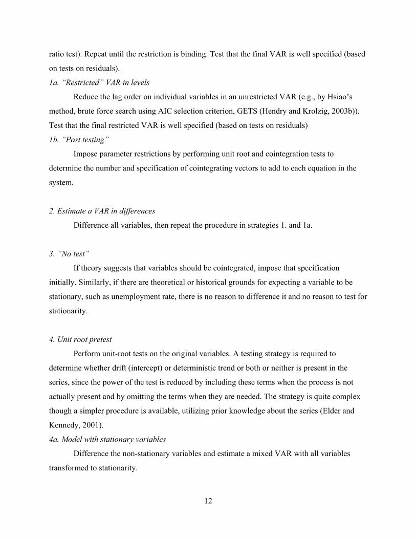
ratio test). Repeat until the restriction is binding. Test that the final VAR is well specified (based

on tests on residuals).

1a. “Restricted” VAR in levels

Reduce the lag order on individual variables in an unrestricted VAR (e.g., by Hsiao’s

method, brute force search using AIC selection criterion, GETS (Hendry and Krolzig, 2003b)).

Test that the final restricted VAR is well specified (based on tests on residuals)

1b. “Post testing”

Impose parameter restrictions by performing unit root and cointegration tests to

determine the number and specification of cointegrating vectors to add to each equation in the

system.

2. Estimate a VAR in differences

Difference all variables, then repeat the procedure in strategies 1. and 1a.

3. “No test”

If theory suggests that variables should be cointegrated, impose that specification

initially. Similarly, if there are theoretical or historical grounds for expecting a variable to be

stationary, such as unemployment rate, there is no reason to difference it and no reason to test for

stationarity.

4. Unit root pretest

Perform unit-root tests on the original variables. A testing strategy is required to

determine whether drift (intercept) or deterministic trend or both or neither is present in the

series, since the power of the test is reduced by including these terms when the process is not

actually present and by omitting the terms when they are needed. The strategy is quite complex

though a simpler procedure is available, utilizing prior knowledge about the series (Elder and

Kennedy, 2001).

4a. Model with stationary variables

Difference the non-stationary variables and estimate a mixed VAR with all variables

transformed to stationarity.

12

4b. Unit root and cointegration pretest

Use the information on non-stationary variables to conduct cointegration tests, impose

the parameter restrictions (if any) that follow from the testing, and estimate the resulting error-

correction model. This strategy is followed by ModelBuilder (Kurcewicz, 2002).

Conflicting advice from the experts – a controversial principle?

As we argued in the introduction, an important aim in developing a methodology should be that

it has an explicit and agreed core on which experts and the supporting evidence agree.

Unfortunately, where the use of unit roots and cointegration is concerned “Experts differ in the

advice offered for applied work”, (Hamilton, 1994, p. 652). In fact, experts, at least those who

write books on the subject, seem unwilling to offer much explicit advice at all. Hendry is an

obvious exception (Hendry, 1995, Hendry, 2002). But where experts are willing to commit

themselves, let us identify the breadth of their disagreement and see if there are any central

principles where agreement is to be found.

Hamilton follows a typical economist’s style, suggesting on the one hand you could estimate in

levels (strategy 1 or 1a), but on the other hand you could estimate in differences (since what is an

ECM but a VAR in differences with some cointegrating vectors tacked on) (strategy 2), while on

the third hand you could pursue a middle ground and do some unit root testing to see how to

enter each variable into the model (strategy 4a).

Harvey is one of the strongest proponents of strategy 3 (no tests), an exemplar of forecasters who

favor state-space and time-varying-parameter approaches who regularly practice the strategy. He

observes (Harvey, 1997, p. 196): “[M]uch of the time, it [unit root testing] is either unnecessary

or misleading, or both”. As well as doubting the value of unit root testing, Harvey has little

enthusiasm for either vector autoregressions or their modification to embody cointegration

restrictions, in part because the modeling strategies (1a, 1b) depend on tests with poor statistical

properties. He continues (p. 199):

13

“However, casting these technical considerations aside, what have economists learnt from

fitting such models? The answer is very little. I cannot think of one article which has come

up with a co-integrating relationship which we did not know already from economic theory.

Furthermore, when there are two or more co-integrating relationships, they can only be

identified by drawing on economic knowledge. All of this could be forgiven if the VECM

provided a sensible vehicle for modeling the short run, but it doesn’t because vector

autoregressions confound long run and short run effects.”

Harvey is being a little unreasonable here. Most VAR modelers try to pick a set of variables that

are connected according to economic theory. It should then be unsurprising if they turn out to be

cointegrated. What is sometimes surprising, given the power problems with cointegration tests

based on the null of restricted models (i.e. with many unit roots imposed) is that they should

sometimes detect the presence of more than one cointegrating vector. Even with economic

knowledge, the argument as to why a set of variables should contain several cointegrating

vectors can be difficult to make.

Harvey’s remarks quoted above stand in sharp contrast to his earlier views, which appear to

recommend strategy 4a:

“Before starting to build a model with explanatory variables, it is advisable to fit a

univariate model to the dependent variable. . . . it provides a description of the salient

features of the series, the ‘stylized facts’ . . . An initial analysis of the potential explanatory

variables may also prove helpful. . . . In particular the order of integration of the variables

will be known. It is not difficult to see that, if the model is correctly specified, the order of

integration of the dependent variable cannot be less than the order of integration of any

explanatory variable. This implies that certain explanatory variables may need to be

differenced prior to their inclusion in the model. A further point is that if the order of

integration of the dependent variable is greater than that of each of the explanatory

variables, a stochastic trend component must be present.” (Harvey, 1990, p.390)

14

Diebold (1998, p. 254) also seems to be arguing for strategy 4a: “In light of the special

properties of series with unit roots, it is sometimes desirable to test for their presence, with an

eye towards the desirability of imposing them, by differencing the data, if they seem to be

present.” But then has second thoughts as to their worth, leaning towards strategy 3: “Thus,

although unit-root tests are sometimes useful, don’t be fooled into thinking they are the end of

the story in regard to the decision of whether to specify models in levels or differences.”

(Diebold, 1998, p. 260).

More arguments favoring strategy 4a come from Stock and Watson (2003, pp. 466-467):

“The most reliable way to handle a trend in a series is to transform the series so that it does

not have a trend. . . .Even though failure to reject the null hypothesis of a unit root does not

mean the series has a unit root, it still can be reasonable to approximate the true

autoregressive root as equaling one and therefore to use differences of the series rather than

its levels.”

Holden also probably favours strategy 4a, though he creates additional concern by mentioning

cointegration:

“When the variables are not stationary . . . [and if] they are not cointegrated the correct

approach is to transform the variables to become stationary . . . and then estimate the VAR

in the usual way.” (Holden ,1995, p. 164)

Rather weakly, (Maddala and Kim, 1998, p. 146) apparently favor strategy 4b:

“[I]t is important to ask the question (rarely asked): why are we interested in testing for unit

roots? Much of this chapter (as is customary) is devoted to the question ‘How do we use unit

root tests?’ rather than ‘Why unit root tests?’ . . . One answer is that you need the unit root

tests as a prelude to cointegration analysis. . .”

Only strategy 2, ‘Estimate in differences’ seems to have been neglected, though Siegert (1999)

(in an attempt to apply the LSEM in modeling the demand for food) adopted this automatically,

much to Hendry’s disgust (Hendry, 1999). But Hendry (1997) himself has noted that when there

are structural breaks, a model that is robust to breaks will tend to produce better forecasts.

Differencing variables imparts robustness, implying that there are conditions when strategy 2

will be the best.

15

Theoretical justification and simulation evidence In theory, when a restriction is true, it should be imposed, since one source of estimation error is

removed. Consequently, if all variables are I(1) and there are no groups of variables that

cointegrate, estimation of a VAR in differences should give a better result and more accurate

forecasts than any less restricted model. Where there are groups of variables that cointegrate,

restrictions that specify one or more cointegrating vectors should give a better result than either a

VAR in differences or a VAR in levels. Imposing restrictions that are not true, for example,

estimating an ECM with one cointegrating vector when there should be two or three should give

a worse result than estimating the more general model. (When the number of cointegrating

vectors is one less than the number of nonstationary variables, this is an equivalent

representation to a VAR in levels.)

Conclusions from Monte Carlo simulations Results of Monte Carlo studies are fairly clear. With a data generating process (DGP) that

contains roots close to unity, and “close to” probably means ≥ .97, a unit root pretest will signal

the presence of a unit root and imposing a unit root will improve forecast accuracy (Diebold and

Kilian, 2000). The assumed DGP is a trending AR(1) process,

, which for ρ=1 (unit root) gives the random walk plus

drift model, for ρ=0 gives the (deterministic) linear trend model, and for values between gives a

mixture of the two models.

1( ( 1t ty t y tα β ρ α β ε−− − = − − − +)) t

Other authors specified a VAR DGP and experimented with imposing several unit roots or near

unit roots on the system. Engle and Yoo (1987) and Clements and Hendry (1995) used

essentially the same model, a two-variable VAR with one lag and one cointegrating vector

imposed. Imposing the cointegration restriction instead of estimation in levels gives better

forecasts, at long horizons, though not at shorter (up to six steps ahead). If forecasts of changes

are wanted, a VAR in differences will be more accurate than VAR in levels, even when the true

model is an ECM (Clements and Hendry, 1995). Reinsel and Ahn (1992) and Lin and Tsay

(1996) used a larger VAR, with four variables and two lags and so were able to generate more

models. These included: clearly stationary, with two near unit roots, with two unit roots (and

16

therefore two cointegrating vectors), and with four unit roots. For the clearly stationary model,

imposing any unit roots worsens the forecast at any horizon. When the largest characteristic

roots are 0.99, imposing four unit roots does not matter much, not the case when the largest roots

are 0.95. In the interesting middle case with two unit roots, most accurate forecasts result from

imposing the correct number of unit roots. Specifying one extra is relatively harmless, while

imposing one fewer is more damaging.

Christoffersen and Diebold (1998) provided an explanation for these findings. The problem with

the comparison of a VAR in levels and an ECM is that the ECM imposes both integration (unit

roots) and cointegration, while the VAR in levels imposes neither. When the DGP contains unit

roots (e.g., cointegrating vectors, differenced variables), and a VAR in levels is estimated, the

estimation errors amplify over time. The VAR in levels is a poor forecaster because it fails to

impose integration (unit roots).

Results hold generally when DGP is in logarithms and estimation is done (incorrectly) using

variables in natural numbers and vice versa. But making the correct transformation (e.g.,

estimating with variables in logs when DGP is in logs) has a much bigger impact on forecast

accuracy than imposing the correct number of unit roots. At least for the one-step ahead forecast

they considered, Chao, Corradi and Swanson (2001) found that estimation in differences gives

more accurate forecasts than estimation in levels (i.e., imposing too many unit roots) when the

DGP is in logs and estimation is in natural numbers. To the extent that the DGP in logs mimics

the non-linearities and breaks found in real-world data, this finding supports the idea that over-

restricting the model gives it robustness.

17

There are some limitations to these Monte Carlo studies. The DGP is very simple. Both DGP and

estimating equation have a fixed parameter structure (no time variation or structural breaks). And

in many of the studies correct lag order is assumed, not tested. Also, unit root and cointegration

tests are not performed. The studies answer the question: Given a system with cointegrated

variables, are more accurate forecasts achieved by imposing more, the correct number, or fewer

than the correct number of restrictions? Except for Diebold and Kilian (2000) they do not answer

the question: Will unit root and cointegration tests reliably tell you the correct specification?

Empirical evidence Despite the voluminous literature on cointegration and unit root testing (growing steadily from

1983 and both peaking, at least temporarily, in 1999 in the Econlit data base at 135 and 106

items respectively) and the accolade of the 2003 Nobel prize, the empirical evidence of its utility

is certainly not voluminous. Table 1 includes only studies that compare the out-of-sample

performance of models. It excludes comparisons with Bayesian VARs in levels or differences or

Bayesian ECMs as falling outside the LSEM methodological framework. A distinction is made

between unrestricted and restricted VARs since the difference does appear to matter.

‘Unrestricted’ means that all variables in all equations have the same lag length. The length is

not necessarily chosen arbitrarily. In four of the seven studies (23 of 35 series) likelihood ratio

tests were used to reduce the lag lengths from the initial choice. Even so, as shown in the first

line of Table 1, further simplification leads to better forecasts, supporting strategy 1a.

A model with variables entered in first differences (strategy 2) tends to give more accurate forecasts

that the same model with the variables in levels (strategy 1), 20 series versus seven, supporting

strategy 2 (“always difference”). Estimation in differences is theoretically correct only when there

are no cointegrating vectors.

Estimating a VAR in levels (strategy 1) versus performing a unit-root pretest and following its

conclusion (usually to a cointegration test and an ECM) appears to have little impact; the strategies

are essentially tied – a surprising result given the emphasis on simplification in the forecasting

literature. Especially surprising, and in conflict with findings from simulations studies, is that

imposing sufficient restrictions to leave one cointegrating vector gives worse results than leaving the

estimation in levels.

On the other hand, the bottom panel of Table 1 is much clearer in supporting the view that

specifying a VAR in differences (strategy 2) is a bad approach compared with arriving at a (less

restrictive) ECM either from theory or through testing. The VAR in differences comes out best when

it should: when there are no cointegrating vectors, and rather surprisingly, in the less restrictive case

when there are three.

18

The effects of structural change Structural change only has relevance in the context of a particular model. The true DGP does not

manifest structural change; the DGP adopted by the modeler and intended to capture the main

effects of the true DGP may well display parameter shifts. Standard unit-root tests (which are

very simple models) do not deal with breaks in the series but have been adapted to do so. One

approach would be to locate the break point and discard the earlier observations, which could

make a test with already low power even less powerful. Better would be to use all the data. The

(single) break may be treated as known (exogenous) or its location discovered by testing.

Multiple breaks can also be specified or tested for. These assumptions place successively more

demands on the data. Where a structural break does exist, use of a standard unit-root test (such as

the augmented Dickey-Fuller test) increases the probability of detecting a unit root in a series

that is actually stationary.

When a break point is specified (in effect, exogenously) a modified form of the ADF test is

needed and the critical values of the limiting test statistic are further in the tails than in the

standard tables (Perron, 1990). Alternatively, the break point(s) can be treated as endogenous to

the data. For data observations t = 1, … , T, with break point at t = m, one approach is to choose

the value of m that gives the least favorable view of the unit root hypothesis. That is, repeat the

test for a range of values of m and select the test statistic with smallest (absolute) value. Zivot

and Andrews (1992) give critical values. Critical values of the limiting test statistic of this form

of the ADF test are even further in the tails than the exogenous break ADF, so it is harder to

reject the null of a unit root when the break is considered endogenous. Simulation studies have

shown that introduction of trend break functions leads to further reductions in power and greater

size distortions (Stock, 1994, p. 2820).

For cointegration testing, similar adaptations have been made. For example, Inoue (1999)

extended the Johansen test to cover structural breaks.

19

Conclusions Each of the strategies identified have advantages and disadvantages, either theoretical or

empirical. The differences arise from the benefits of imposing restrictions when they hold true

out-of-sample compared to the costs if they fail.

Compared to other specifications, Strategy 1, an ‘unrestricted VAR in levels’ avoids throwing

away information (Sims, 1980). Even if the true model is a VAR in differences, hypothesis tests

based on a VAR in levels will have the same asymptotic distribution as if the correct model had

been used. However, it may be overparameterized and give a correspondingly bad forecasts.

But the initial unrestricted model, like all the alternative approaches to model specification, is no

more immune from failing misspecification tests (wrong choice of variables, poor autoregressive

approximation to the true DGP, etc., Harvey, 1997). It also responds slowly to structural breaks.

Comparing the unrestricted VAR with its restricted cousin, the simpler model, following similar

conclusions from univariate comparisons (Fildes and Ord, 2002), proves the more accurate as

Table 1 shows.

The ‘restricted VAR in levels’ specification, strategy 1a, also may ignore data-congruent

restrictions. These derive from long-run equilibrium relationships (cointegration) that would lead

to alternative, even simpler, model structures through ‘post-testing’ strategy 1b. We found no

studies that compared strategies 1 and 1b directly, only comparisons of strategies 1 and

‘pretesting’, 4b. But the empirical evidence of Table 1 offers little support to the view that this

leads to a significant improvement in forecasting. However, the ‘post-testing’ strategy rarely

leads to a VAR in differences, so this remains the preferred strategy since ECMs prove

considerably better than VARs automatically specified in differences (Strategy 2). Strategy 2

also suffers from the problem that if the variables are already stationary, differencing induces a

moving average term into the equation (though how important such a mis-specification is when

estimating the model is an empirical question). And although Monte Carlo studies have shown

that an advantage of specifying a VAR in differences is that it is robust if there are structural

breaks, we found no empirical evidence to support the simulation comparisons.

20

Strategy 3 relies on other means of model specification (such as cointegration relations imposed

from theory). A general model that is theoretically consistent allows specification testing for

nested special cases (e.g., a time-varying parameter model that allows for fixed parameters as

special cases). To support his 1997 argument for this strategy (Harvey, 1997, p.197) Harvey

focuses on the near impossibility of identifying the appropriate order of integration. Empirical

evidence, summarized in Allen and Fildes (2001), suggests that time-varying parameter or state-

space models developed with this strategy forecast better than models developed by other

methods.

There is however a cost to adding in this additional level of generality. Allowing response

parameters to vary over observations increases the chances for misspecification (Judge et al.,

1985, p. 815) and an even larger set of parameters needs to be considered. Consequently, while

the state-space models permit some non-linearities, which might be an important feature, they

typically use a small set of variables and simple dynamics. Fixed-parameter models derived from

them are too simple and easily beaten by the more general varying-parameter model. We found

no comparisons of forecasts from a model developed by conventional general-to-specific

methods (strategies 1b or 4b) with those from a state-space model.

The final arm of Figure 1 relies on pre-tests. The use of unit root pre-tests to ensure a model

specified in stationary variables has the single advantage of achieving a constrained model. But

the tests have low power and might lead to erroneous conclusions about the existence of unit

roots and cointegrating vectors, resulting in a misspecified over-constrained model. Nor are the

constraints necessarily appropriate (consider an ECM model with one cointegrating vector).

21

Assembling the evidence presented so far suggests that a strategy of never testing for unit roots

and cointegration is inferior to testing, even though the tests have admittedly low power. It does

not much matter whether unit-root and cointegration testing is conducted on the variables before

a model is specified or as part of the reduction of an acceptable general model. What does matter

is that the unit-root pretest not be used to establish a set of I(0) variables, by differencing if

necessary, and these variables be entered into a VAR. This is a form of restricted VAR that

should have desirable properties, since all variables are in stationary form, but fails to make use

of the valuable information contained in a cointegrating relationship.

Ideally, tests will give information on the correct number and form of restrictions, so that unit-

root and cointegration restrictions imposed on the final model are those that best describe the

DGP. According to simulation evidence, imposing one more restriction than the correct number

is harmless. This finding is likely to hold with real data where structural breaks are

commonplace and imposing additional unit root restrictions will therefore make the final model

more robust to breaks.

To conclude, the primary aim of this paper has been to establish some clear principles of model

specification for the purposes of forecasting within the LSE methodological framework. The

empirical evidence we have collected has shown convincingly that strategies to sequentially

reduce the general model in levels to a constrained model with either ECM or differenced

variables is beneficial and leads to improved forecasting accuracy. The results are generally in

accord to the predictions derived from cointegration theory. Within the LSE methodology we

can therefore claim to have established a principle that forecasters should build into their

modeling: start with a general model, restrict the lag lengths and use unit root and cointegration

tests (strategies 1b and 4b).

22

The principle just established is unambiguous but conflicts with much of the advice given in the

text books. Nor does it appear to be uniformly true. Further investigation should therefore lead

towards a clearer specification of the conditions under which it holds. The empirical evidence is

not overwhelming and, in some circumstances, is in conflict with the theoretical predictions, e.g.

where an ECM is outperformed by a model specified in levels, even though a cointegrating

vector has been detected. Of course the number of studies involved are small and the results

stochastic. Structural breaks we know to be a factor that leads to the better performance of

differenced model specifications and this may explain the observed results. As the evidence

slowly accumulates on these strategies, with more careful testing of structural breaks, both in and

out-of-sample, as an automatic aspect of specification testing, we can expect this anomaly to be

clarified.

A subsidiary aspect of the paper has been to examine the role of algorithmic versus tacit

knowledge when specifying forecasting models. Kennedy (2002) cites the complaints of several

well-known econometricians: we teach what we know, not the applied econometrics needed for

analysis of messy data; combining often controversial theories with evidence is difficult; the

profession does not appear to value empirical work very highly, relative to theoretical

econometrics work; writing down rules to guide data analysis (and when to ignore them) is hard,

because so much of data analysis is subjective, subtle and a tacit skill. This unsatisfactory state

of affairs is changing, if slowly. Computer algorithms, or expert systems, such as GETS and

ModelBuilder require explicit rules. Tinkering with the computer code and measuring the effect

on outcomes shows the impact of well-defined rules. Perhaps a parallel situation is in the

estimation of ARIMA models. As proposed by Box and Jenkins, considerable experience,

judgment and time were called for to identify, estimate and evaluate such models. Today,

computer algorithms routinely produce models as good as or better than the experts, in a fraction

of the time. Econometric analysis is considerably more involved, but the same progression

should be possible.

The analysis of a wide range of empirical evidence carefully coded has shown its worth, when

interpreted through econometric theory. Potential anomalies have been identified suggesting

areas of future research. Such an approach has the potential for driving downward Pagan’s

“uncomfortably high art-to-science ratio”.

References Allen, P. G. and Fildes, R. (2001). Econometric forecasting. In J. Scott Armstrong (editor), Principles of Forecasting: A Handbook for Researchers and Practitioners, pp. 303-362, Kluwer Academic Press, Norwell, MA. Armstrong, J.S. (2001). Introduction. In J. Scott Armstrong (editor), Principles of Forecasting: A Handbook for Researchers and Practitioners, pp. 1-14, Kluwer Academic Press, Norwell, MA. Banerjee, A., Galbraith, J.W. and Dolado, J. (1990). Dynamic specification and linear transformations of the autoregressive-distributed lag model. Oxford Bulletin of Economics and Statistics, 52, 95-104. 23

Chao, J.C., Corradi, V. and Swanson, N.R. (2001). Data transformation and forecasting in models with unit roots and cointegration. Annals of Economics and Finance, 2, 59-76. Christoffersen, P.F. and Diebold F.X. (1998). Cointegration and long-horizon forecasting. Journal of Business and Economic Statistics, 16, 450-458. Clements, M.P. and Hendry, D.F. (1995). Forecasting in cointegrated systems. Journal of Applied Econometrics, 10, 127-146. Clements, M.P. and Hendry D.F. (1998). Forecasting Economic Time Series. Cambridge University Press, Cambridge. Collins H.M. (1990). Artificial Experts. Social Knowledge and Intelligent Machines, MIT Press, Cambridge, MA. Darnell, A. C. and Evans, J. L. (1990). The Limits of Econometrics. Elgar, Aldershot, U.K. Dewald, W.G., Anderson, R.G. and Thursby, J.G. (1986). Replication in empirical economics: the Journal of Money, Credit and Banking project. American Economic Review, 76, 587-603. Dharmapala, D., and McAleer, M. (1996). Econometric methodology and the philosophy of science. Journal of Statistical Planning and Inference, 49, 9-37. Diebold, F.X. (1998). Elements of Forecasting. South-Western College Publishing, Cincinnati, Ohio. Diebold, F.X. and Kilian, L. (2000). Unit Root Tests are Useful for Selecting Forecasting Models. Journal of Business and Economic Statistics, 18, 265-273. Elder, J. and Kennedy, P. E. (2001). Testing for unit roots: what should students be taught? Journal of Economic Education, 32, 137-146. Engle, R.F. and Yoo B.S. (1987). Forecasting and testing in co-integrated systems. Journal of Econometrics, 35, 143-159. Fildes, R., and Ord, J.K. (2002). Forecasting competitions – their role in improving forecasting practice and research, in: A Companion to Economic Forecasting, M. Clements and D. Hendry (eds.), Oxford, Blackwell, 2002, 322-353. Hamilton, J.D. (1994). Time Series Analysis. Princeton University Press, Princeton NJ. Harvey, A. C. (1990). Forecasting, Structural Time Series Models and the Kalman Filter, Cambridge University Press, Cambridge, England. Harvey, A. (1997). Trends, cycles and autoregressions. Economic Journal, 107, 192-201. 24

Hendry, D.F. (1995), Dynamic Econometrics, Oxford University Press, Oxford. Hendry, D.F. (1997). The econometrics of macroeconomic forecasting. Economic Journal, 107, 1330-1357. Hendry, D.F. (1999). An econometric analysis of US food expenditure. In J.R. Magnus and M.S. Morgan (Eds.) Methodology and Tacit Knowledge, pp. 341-361. Wiley, Chichester, UK. Hendry, D.F. (2002). Applied econometrics without sinning. Journal of Economic Surveys, 16, 591-604. Hendry, D.F. and Anderson, G.J. (1977). Testing dynamic specification in small simultaneous models: and application to a model of building society behaviour in the United Kingdom. In M.D. Intrilligator (Ed.) Frontiers of Quantitative Economics, vol. IIIA. North-Holland, Amsterdam. Hendry, D.F. and Krolzig, H-M. (2003a) New developments in automatic general-to-specific modeling, in Stigum, B. P. Econometrics and the Philosophy of Economics: Theory-Data Confrontations in Economics, Princeton University Press, Princeton, NJ. Hendry, D.F. and Krolzig, H-M. (2003b). The Properties of Automatic Gets Modeling. Nuffield College Economics Working Papers 2003-W14. http://www.nuff.ox.ac.uk/economics/papers/2003/W14/dfhhmk03a.pdf Holden, K. (1995). Vector autoregression modeling and forecasting. Journal of Forecasting, 14, 159-166. Hoover, K.D., and Perez, S.J. (1999). Data mining reconsidered: encompassing and the general-to-specific approach to specification searches. Econometrics Journal, 2, 167-191. Inoue, A. (1999). Tests of cointegrating rank with a trend-break. Journal of Econometrics, 90, 215–237. Johansen, S. (1988). Statistical analysis of cointegration vectors. Journal of Economic Dynamics and Control, 12, 231-254. Judge, G. G., W. E. Griffiths, R. C. Hill, H. Lütkepohl, and T.C. Lee (1985), The Theory and Practice of Econometrics, (2nd ed.), Wiley, New York. Kennedy, P.E. (2002). Sinning in the basement: What are the rules? The ten commandments of applied econometrics. Journal of Economic Surveys, 16, 569-589. Kurcewicz, M. (2002). ModelBuilder - an automated general-to-specific modeling tool. In Haerdle, W. and Roenz, B. (eds.) Compstat 2002 - Proceedings in Computational Statistics, pp. 467-472, Physica-Verlag, Heidelberg.

25

Leamer, E.E. (1983). Let's take the con out of econometrics. American Economic Review, 73, 31-43. Leamer, E.E. (1999). Revisiting Tobin's 1950 study of food expenditure. In J.R. Magnus and M.S. Morgan (Eds.) Methodology and Tacit Knowledge, pp. 315-340. Wiley, Chichester, UK. Lin, J-L. and Tsay, R.S. (1996). Co-integration constraint and forecasting: an empirical examination. Journal of Applied Econometrics, 11, 519-538. Maddala, G.S. and Kim, I-M. (1998). Unit roots, Cointegration, and Structural Change, Cambridge University Press, Cambridge, England. Magnus, J.R., and Morgan, M.S. (1999a). Methodology and Tacit Knowledge. (Eds.) Wiley, Chichester, UK. Magnus, J.R., and Morgan, M.S. (1999b). Lessons from the tacit knowledge experiment. In J.R. Magnus and M.S. Morgan (Eds.) Methodology and Tacit Knowledge, pp. 375-381. Wiley, Chichester, UK. Magnus, J.R., and Morgan, M.S. (1999c). Lessons from the field trial experiment. In J.R. Magnus and M.S. Morgan (Eds.) Methodology and Tacit Knowledge, pp. 302-307. Wiley, Chichester, UK. Pagan, A.R. (1987). Three econometric methodologies: a critical appraisal. Journal of Economic Surveys, 1, 3-24. Pagan, A.R. (1999). The Tilburg experiments: impressions of a drop-out. In J.R. Magnus and M.S. Morgan (Eds.) Methodology and Tacit Knowledge, pp. 369-374. Wiley, Chichester, UK. Perron, P. (1990). Testing for a unit root in a time series with a changing mean. Journal of Business and Economic Statistics, 8, 153-62. Reinsel, G.C. and Ahn, S.K. (1992). Vector autoregressive models with unit roots and reduced rank structure: estimation, likelihood ratio test and forecasting. Journal of Time Series Analysis, 13, 353-375. Siegert, W.K. (1999). An application of three econometric methodolgies to the estimation of income elasticity of food demand. In J.R. Magnus and M.S. Morgan (Eds.) Methodology and Tacit Knowledge, pp. 315-340. Wiley, Chichester, UK. Sims, C.A. (1980). Macroeconomics and reality. Econometrica, 48, 1-48. Stock, J.H. (1994). Unit roots, structural breaks and trends. Handbook of Econometrics, Vol. 4, Chapter 46, 2739-2841.

26

Stock, J.H. (1996). VAR, error correction and pretest forecasts at long horizons. Oxford Bulletin of Economics and Statistics, 58, 685-701. Stock, J.H. and Watson, M.K. (2003). Introduction to Econometrics. Addison-Wesley, Boston MA Zellner, A. (2004) Statistics, Econometrics and Forecasting, Cambridge University Press, Cambridge. Zivot, E. and Andrews, D.W.K. (1992). Further evidence on the great crash, the oil-price shock, and the unit-root hypothesis. Journal of Business and Economic Statistics, 20, 25-44.

27

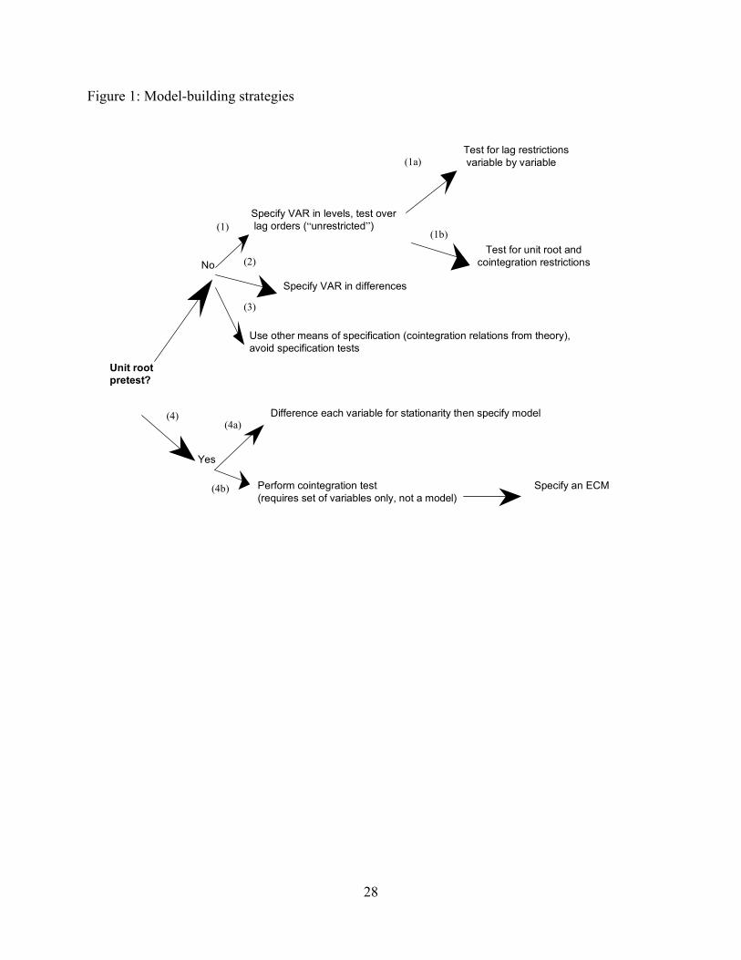
Figure 1: Model-building strategies

Difference each variable for stationarity then specify model

Yes

No

Perform cointegration test (requires set of variables only, not a model)

Unit rootpretest?

Specify VAR in levels, test overlag orders (“unrestricted”)

Test for lag restrictionsvariable by variable

Test for unit root andcointegration restrictions

Use other means of specification (cointegration relations from theory), avoid specification tests

Specify VAR in differences

Specify an ECM

(1)

(2)

(1b)

(1a)

(3)

(4)

(4b)

(4a)

28

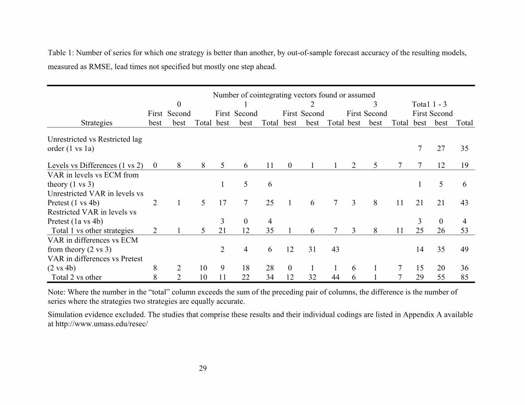
Table 1: Number of series for which one strategy is better than another, by out-of-sample forecast accuracy of the resulting models,

measured as RMSE, lead times not specified but mostly one step ahead.

Number of cointegrating vectors found or assumed 0 1 2 3 Tota1 1 - 3

Strategies First best

Second best Total

First best

Second best Total

First best

Second best Total

First best

Second best Total

First best

Second best Total

Unrestricted vs Restricted lag order (1 vs 1a) 7 27 35

Levels vs Differences (1 vs 2) 0 8 8 5 6 11 0 1 1 2 5 7 7 12 19 VAR in levels vs ECM from theory (1 vs 3) 1 5 6 1 5 6 Unrestricted VAR in levels vs Pretest (1 vs 4b) 2 1 5 17 7 25 1 6 7 3 8 11 21 21 43 Restricted VAR in levels vs Pretest (1a vs 4b) 3 0 4 3 0 4 Total 1 vs other strategies 2 1 5 21 12 35 1 6 7 3 8 11 25 26 53 VAR in differences vs ECM from theory (2 vs 3) 2 4 6 12 31 43 14 35 49 VAR in differences vs Pretest (2 vs 4b) 8 2 10 9 18 28 0 1 1 6 1 7 15 20 36 Total 2 vs other 8 2 10 11 22 34 12 32 44 6 1 7 29 55 85

Note: Where the number in the “total” column exceeds the sum of the preceding pair of columns, the difference is the number of series where the strategies two strategies are equally accurate.

Simulation evidence excluded. The studies that comprise these results and their individual codings are listed in Appendix A available at http://www.umass.edu/resec/

29

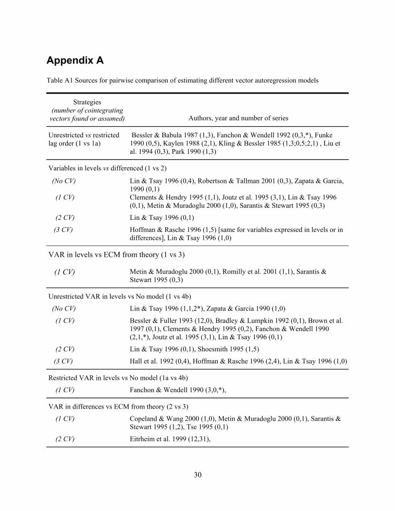
Appendix A Table A1 Sources for pairwise comparison of estimating different vector autoregression models

Strategies (number of cointegrating

vectors found or assumed)

Authors, year and number of series

Unrestricted vs restricted lag order (1 vs 1a)

Bessler & Babula 1987 (1,3), Fanchon & Wendell 1992 (0,3,*), Funke 1990 (0,5), Kaylen 1988 (2,1), Kling & Bessler 1985 (1,3;0,5;2,1) , Liu et al. 1994 (0,3), Park 1990 (1,3)

Variables in levels vs differenced (1 vs 2)

(No CV)

Lin & Tsay 1996 (0,4), Robertson & Tallman 2001 (0,3), Zapata & Garcia, 1990 (0,1)

(1 CV) Clements & Hendry 1995 (1,1), Joutz et al. 1995 (3,1), Lin & Tsay 1996 (0,1), Metin & Muradoglu 2000 (1,0), Sarantis & Stewart 1995 (0,3)

(2 CV) Lin & Tsay 1996 (0,1)

(3 CV) Hoffman & Rasche 1996 (1,5) [same for variables expressed in levels or in differences], Lin & Tsay 1996 (1,0)

VAR in levels vs ECM from theory (1 vs 3)

(1 CV) Metin & Muradoglu 2000 (0,1), Romilly et al. 2001 (1,1), Sarantis & Stewart 1995 (0,3)

Unrestricted VAR in levels vs No model (1 vs 4b)

(No CV) Lin & Tsay 1996 (1,1,2*), Zapata & Garcia 1990 (1,0)

(1 CV) Bessler & Fuller 1993 (12,0), Bradley & Lumpkin 1992 (0,1), Brown et al. 1997 (0,1), Clements & Hendry 1995 (0,2), Fanchon & Wendell 1990 (2,1,*), Joutz et al. 1995 (3,1), Lin & Tsay 1996 (0,1)

(2 CV) Lin & Tsay 1996 (0,1), Shoesmith 1995 (1,5)

(3 CV) Hall et al. 1992 (0,4), Hoffman & Rasche 1996 (2,4), Lin & Tsay 1996 (1,0)

Restricted VAR in levels vs No model (1a vs 4b)

(1 CV) Fanchon & Wendell 1990 (3,0,*),

VAR in differences vs ECM from theory (2 vs 3)

(1 CV) Copeland & Wang 2000 (1,0), Metin & Muradoglu 2000 (0,1), Sarantis & Stewart 1995 (1,2), Tse 1995 (0,1)

(2 CV) Eitrheim et al. 1999 (12,31),

30

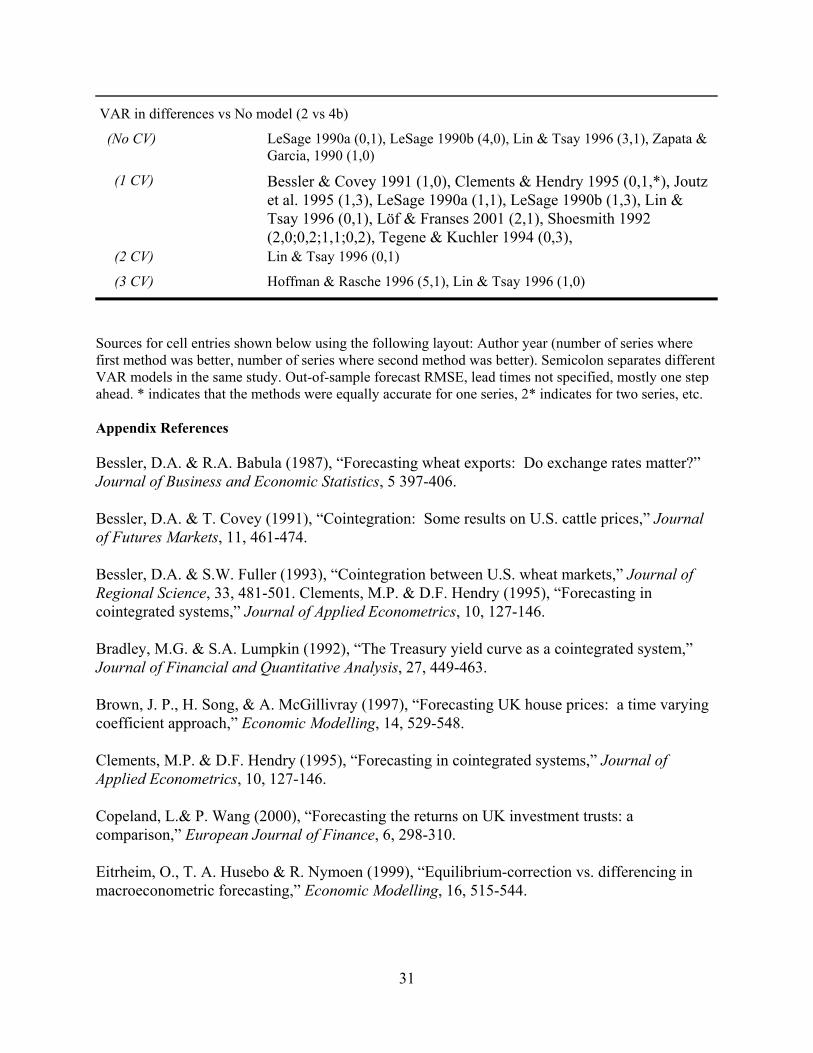
VAR in differences vs No model (2 vs 4b)

(No CV) LeSage 1990a (0,1), LeSage 1990b (4,0), Lin & Tsay 1996 (3,1), Zapata & Garcia, 1990 (1,0)

(1 CV) Bessler & Covey 1991 (1,0), Clements & Hendry 1995 (0,1,*), Joutz et al. 1995 (1,3), LeSage 1990a (1,1), LeSage 1990b (1,3), Lin & Tsay 1996 (0,1), Löf & Franses 2001 (2,1), Shoesmith 1992 (2,0;0,2;1,1;0,2), Tegene & Kuchler 1994 (0,3),

(2 CV) Lin & Tsay 1996 (0,1)

(3 CV) Hoffman & Rasche 1996 (5,1), Lin & Tsay 1996 (1,0)

Sources for cell entries shown below using the following layout: Author year (number of series where first method was better, number of series where second method was better). Semicolon separates different VAR models in the same study. Out-of-sample forecast RMSE, lead times not specified, mostly one step ahead. * indicates that the methods were equally accurate for one series, 2* indicates for two series, etc. Appendix References Bessler, D.A. & R.A. Babula (1987), “Forecasting wheat exports: Do exchange rates matter?” Journal of Business and Economic Statistics, 5 397-406. Bessler, D.A. & T. Covey (1991), “Cointegration: Some results on U.S. cattle prices,” Journal of Futures Markets, 11, 461-474. Bessler, D.A. & S.W. Fuller (1993), “Cointegration between U.S. wheat markets,” Journal of Regional Science, 33, 481-501. Clements, M.P. & D.F. Hendry (1995), “Forecasting in cointegrated systems,” Journal of Applied Econometrics, 10, 127-146. Bradley, M.G. & S.A. Lumpkin (1992), “The Treasury yield curve as a cointegrated system,” Journal of Financial and Quantitative Analysis, 27, 449-463. Brown, J. P., H. Song, & A. McGillivray (1997), “Forecasting UK house prices: a time varying coefficient approach,” Economic Modelling, 14, 529-548. Clements, M.P. & D.F. Hendry (1995), “Forecasting in cointegrated systems,” Journal of Applied Econometrics, 10, 127-146. Copeland, L.& P. Wang (2000), “Forecasting the returns on UK investment trusts: a comparison,” European Journal of Finance, 6, 298-310. Eitrheim, O., T. A. Husebo & R. Nymoen (1999), “Equilibrium-correction vs. differencing in macroeconometric forecasting,” Economic Modelling, 16, 515-544.

31

Fanchon, P. & J. Wendell (1992), “Estimating VAR models under non-stationarity and cointegration: Alternative approaches to forecasting cattle prices,” Applied Economics, 24, 207-217. Funke, M. (1990), “Assessing the forecasting accuracy of monthly vector autoregressive models: The case of five OECD Countries,” International Journal of Forecasting, 6, 363-378. Hall, A.D., H.M. Anderson & C.W.J. Granger (1992), “A cointegration analysis of Treasury bill yields,” Review of Economics and Statistics, 74, 116-126. Hoffman, D.L. & R.H. Rasche (1996), “Assessing forecast performance in a cointegrated system,” Journal of Applied Econometrics, 11, 495-517. Joutz, F.L., G.S. Maddala, & R.P. Trost (1995), “An integrated Bayesian vector autoregression and error correction model for forecasting electricity consumption and prices,” Journal of Forecasting, 14, 287-310. Kaylen, M.S. (1988), “Vector autoregression forecasting models: Recent developments applied to the U.S. hog market,” American Journal of Agricultural Economics, 70, 701-712. Kling, J.L. & D.A. Bessler (1985), “A comparison of multivariate forecasting procedures for economic time series,” International Journal of Forecasting, 1, 5-24. LeSage, J.P. (1990a), “A comparison of the forecasting ability of ECM and VAR models,” Review of Economics and Statistics, 72, 664-671. LeSage, J.P. (1990b), “Forecasting turning points in metropolitan employment growth rates using Bayesian techniques,” Journal of Regional Science, 30, 533-548. Lin, J-L. & R.S. Tsay (1996), “Co-integration constraint and forecasting: an empirical examination,” Journal of Applied Econometrics, 11, 519-538. Liu, T-R., M.E. Gerlow & S.H. Irwin (1994), The performance of alternative VAR models in forecasting exchange rates,” International Journal of Forecasting, 10, 419-433. Löf, M & P.H. Franses (2001), “On forecasting seasonal time series,” International Journal of Forecasting, 17, 607-621. Metin, K. & G. Muradoğlu (2000), “Forecasting stock prices by using alternative time series models,” ISE Review, 4, 17-24. Park, T. (1990), “Forecast evaluation for multivariate time-series models: The U.S. cattle market,” Western Journal of Agricultural Economics, 15, 133-143.

32

Robertson, J. C. & E. W. Tallman (2001), “Improving federal-funds rate forecasts in VAR models used for policy analysis,” Journal of Business and Economic Statistics, 19, 324-330.

33

Romilly, P., H. Song & X. Liu (2001), “Car ownership and use in Britain: a comparison of the empirical results of alternative cointegration estimation methods and forecasts,” Applied Economics, 33, 1803-1818. Sarantis, N. & C. Stewart (1995), “Structural, VAR and BVAR models of exchange rate determination: A comparison of their forecasting performance,” Journal of Forecasting, 14, 201-215. Shoesmith, G.L. (1992), “Cointegration, error correction, and improved medium-term regional VAR forecasting,” Journal of Forecasting, 11, 91-109. Shoesmith, G.L. (1995), “Multiple cointegrating vectors, error correction, and forecasting with Litterman's model,” International Journal of Forecasting, 11, 557-67. Tegene, A. & F. Kuchler (1994), “Evaluating forecasting models of farmland prices,” International Journal of Forecasting, 10, 65-80. Tse, Y.K. (1995), “Lead-lag relationship between spot index and futures price of the Nikkei stock average,” Journal of Forecasting, 14, 553-563. Zapata, H.O. & P. Garcia (1990), “Price forecasting with time-series methods and nonstationary data: An application to monthly U.S. cattle prices,” Western Journal of Agricultural Economics, 15, 123-132.