Czech Technical University in Prague

Faculty of Nuclear Sciences andPhysical Engineering

Department of Physics

MASTER THESIS

Application of antiprotons forradiotherapy

(Studium vyuzitı antiprotonu pro radioterapii)

Praha, 2006 Hedvika Toncrova

Nazev prace: Studium vyuzitı antiprotonu pro radioterapii

Autor: Toncrova Hedvika

Obor: Matematicke inzenyrstvı

Druh prace: Diplomova prace

Vedoucı prace: RNDr.Vojtech Petracek, CSc., Katedra fyziky, Fakulta

jaderna a fyzikalne inzenyrska, Ceske vysoke ucenı tech-

nicke v Praze

Konzultant: Dr.Michael Doser, CERN, Svycarsko

II

Prohlasuji, ze jsem svou diplomovou praci vypracovala samostatne a pouzila

jsem pouze podklady ( literaturu, projekty, SW atd.) uvedene v prilozenem sez-

namu.

Nemam zavazny duvod proti uzitı tohoto skolnıho dıla ve smyslu § 60 Zakona

c.121/2000 Sb. , o pravu autorskem, o pravech souvisejıcıch s pravem autorskym a

o zmene nekterych zakonu (autorsky zakon).

I declare that I have written this diploma thesis independently using the listed

references. I agree with using this diploma thesis.

V Praze dne

Hedvika Toncrova

III

Acknowledgement

I would like to express my gratitude to all those who gave me the possibility to

complete this thesis. I want to thank my CERN supervisor Dr.Michael Doser, for

involving me in the project and helping me throughout the initial phases of the

work. The summer at CERN was an unforgettable period of my life.

I am deeply grateful to my supervisor, RNDr.Vojtech Petracek, for his detailed

and constructive comments, and for his important support throughout this work.

I also wish to thank Jamie (super damn cool) Tattersall, who looked closely at

the final version of the thesis for English style and grammar, correcting both and

offering suggestions for improvement.

Especially, I would like to give my special thanks to my parents whose endless

patience and love enabled me to complete this work.

IV

Abstrakt

Vyuzitı antiprotonu pro radioterapii predstavuje alternativu k tradicnım radiotera-

peutickym metodam a zda se ze je i v mnoha ohledech vyhodnejsı. Vysledky prvnıch

experimentu totiz naznacujı ze jejich biologicka ucinnost je az ctyrikrat vyssı nez bio-

logicka ucinnost protonu, v soucasne dobe jednech z nejucinejsıch castic pouzıvanych

v radioterapii. Dalsım potencialnım prınosem antiprotonu je moznost zobrazit

rozlozenı mıst anihilacı v prostoru pomocı vysokoenergetickych castic vyzarenych

z mısta anihilace. V idealnım prıpade by tato zobrazovacı metoda byla pouzita

pred samotnou terapiı k overenı terapeutickeho planu a pote ke kontrole prubehu

vlastnıho ozarovanı.

Navrzeny terapeuticky plan by mohl byt overen ozarenım pacienta zkusebnım

paprskem o nızke intenzite, ktery by byl nasledovan plnou davkou. V prubehu

plneho ozarovanı muze zobrazovacı zarızenı slouzit pro zpetnou vazbu. To by

mohlo predstavovat velkou vyhodu teto metody, zejmena pro nadory ulozene v

blızkosti citlivych oblastı. Prvnı experiment, ktery zkoumal moznosti zobrazovanı

byl proveden na antiprotonovem dekcelratoru v CERNu a dalsi budou v blızke dobe

nasledovat.

Prvnı kapitoly teto prace jsou venovany historii radioterapie a fyzikalnım prin-

cipum, ktere jsou pri nı vyuzıvany. Cast je tvorena rychlym prehledem experimentu,

ktere zkoumaly interakci antiprotonu s biologickymi tkanemi. Samostatna kapi-

tola je venovana vyse zmınenemu experimentu, ktery testoval moznosti zobrazenı

cıloveho objemu zarenı. Bohuzel behem experimentu doslo k selhanı nektereho z

prıstroju a tak jsou data z experimentu neuplna a tudız nemohla byt analyzovana. Je

vsak ukazano ze velikost cıloveho objemu muze byt rekonstuovana jen velmi priblizne

s pouzitym experimentalnım usporadanım. Proto je nejvetsı cast teto prace zamere-

na na navrh vylepseneho usporadanı, ktere je citlivejsı k parametrum prostoroveho

rozlozenı anihilacı. Jsou navrzena dve experimentalnı usporadanı a jejich chovanı je

simulovano. Program, ktery z namerenych hodnot rekonstruuje puvodnı distribuci

je popsan a vysledky predstaveny. Navrzena usporadanı jsou velmi jednoducha aby

se ulehcila jejich instalace v prostorach antiprotonoveho dekceleratoru. Nicmene

rekonstrukce je pomerne presna a tak by zakladnı myslenka mohla najıt uplatnenı i

v budoucıch klinickych aplikacıch.

Klıcova slova: antiprotony, radioterapie.

V

Abstract

Antiprotons offer an alternative to established radiotherapeutic methods. Initial

trial experiments indicates that the biological efficiency of antiprotons is up to four

times higher than that of protons, currently one of the most efficient particles used

in radiotherapy. Another potential benefit of antiprotons is the possibility to image

the stopping distribution using the high energy particles that emanate from the

annihilation vertex. Optimally the imaging would be used at first to confirm a

therapy plan and later to control the course of irradiation.

A therapy plan can be confirmed with a low intensity beam before the patient

is irradiated with a therapeutical dose. In the course of the irradiation the imaging

device can serve as a control system. This could be a great advantage, especially for

tumors located close to sensitive areas. A first experiment to test the possibilities

of the imaging was carried out at the AD facility at CERN and other experiments

will follow in forthcoming beam time.

The first chapters of this thesis are devoted to a history of radiotherapy and

its physical principles. A part of it is a quick review of important experiments

testing the interaction of antiprotons with biological tissues. The next chapter

describes the experiment which tested the real time imaging. Unfortunately during

the experiment a failure of technical devices caused the data acquired from the

experiment to be incomplete and it cannot be used for analysis. It is shown that

only the bulk properties of the stopping distribution could be reconstructed with the

experimental design used. Therefore a main part of this thesis refers to a proposal

for an improved experiment which is more sensitive to the parameters of the stopping

distribution. Two experimental designs are proposed and its performance simulated.

The program that reconstructs the stopping distribution from the acquired data is

described and its results presented. The designs are very simple in order to facilitate

the installation of the experiment in the area of the AD. The reconstruction, however

is fairly precise and therefore the main idea of the design could be used in clinical

applications.

Keywords: antiprotons, radiotherapy.

VI

Contents

1 Introduction 1

2 Radiotherapy 3

2.1 Studies of antiprotons for radiotherapy . . . . . . . . . . . . . . . . . 5

2.2 Imaging . . . . . . . . . . . . . . . . . . . . . . . . . . . . . . . . . . 8

3 Principles of beam therapy 10

3.1 Lateral scattering . . . . . . . . . . . . . . . . . . . . . . . . . . . . . 12

3.2 Conformal beam treatment . . . . . . . . . . . . . . . . . . . . . . . . 12

3.3 Annihilation . . . . . . . . . . . . . . . . . . . . . . . . . . . . . . . . 13

3.4 Monte Carlo Simulation . . . . . . . . . . . . . . . . . . . . . . . . . 16

4 The Prototype Experiment and its Analysis 20

4.1 GEANT4 simulation . . . . . . . . . . . . . . . . . . . . . . . . . . . 22

4.2 Algorithm for the experiment analysis . . . . . . . . . . . . . . . . . . 23

4.3 Conclusion . . . . . . . . . . . . . . . . . . . . . . . . . . . . . . . . . 29

5 Proposal For The Next Experiment 30

5.1 A layout using two detector sets . . . . . . . . . . . . . . . . . . . . . 31

5.2 A layout using three detector sets . . . . . . . . . . . . . . . . . . . . 36

6 Conclusions and further perspectives 42

A Program for the reconstruction 45

Bibliography 46

VII

List of Figures

2.1 Survival of V79 Chinese Hamster cells . . . . . . . . . . . . . . . . . 6

2.2 Measured profile of the dose deposition in a phantom . . . . . . . . . 7

2.3 Survival for Peak and Plateau regions . . . . . . . . . . . . . . . . . . 8

3.1 Comparison of depth dose profiles for various particles . . . . . . . . 11

3.2 Cross sections of pp . . . . . . . . . . . . . . . . . . . . . . . . . . . . 13

3.3 Cross sections of pd and pn . . . . . . . . . . . . . . . . . . . . . . . 14

3.4 P-wave annihilation as a function of density . . . . . . . . . . . . . . 15

3.5 Pion spectrum . . . . . . . . . . . . . . . . . . . . . . . . . . . . . . . 16

3.6 Energy deposition of a stopping antiproton . . . . . . . . . . . . . . . 17

3.7 Momentum spectra of the pions created during a simulated annihilation. 18

3.8 Momentum spectra of the p, n and α created during a simulated

annihilation. . . . . . . . . . . . . . . . . . . . . . . . . . . . . . . . . 19

4.1 The scheme of PS experiments including the AD ring. . . . . . . . . . 20

4.2 AD cycle. . . . . . . . . . . . . . . . . . . . . . . . . . . . . . . . . . 21

4.3 Experimental setup used to test the real-imaging . . . . . . . . . . . 22

4.4 An annihilation event generated by Geant4. . . . . . . . . . . . . . . 23

4.5 Stopping distribution of antiprotons in water as a function of pene-

tration depth, simulated with Geant4. . . . . . . . . . . . . . . . . . . 26

4.6 Reconstruction of experiment in the x and y direction . . . . . . . . . 28

5.1 A scheme of first proposed experimental design. Top view. . . . . . . 32

5.2 Stopping distribution of monoenergetic antiprotons along the beam

axis . . . . . . . . . . . . . . . . . . . . . . . . . . . . . . . . . . . . . 33

5.3 Reconstructed range profile of spread-out Bragg peaks . . . . . . . . 34

5.4 Stopping distribution of antiprotons, transverse to the beam . . . . . 35

5.5 Occupancy of a parallel and a perpendicular detector . . . . . . . . . 36

5.6 A scheme of the proposed 3 detector design . . . . . . . . . . . . . . 37

VIII

5.7 Transverse beam profile reconstructed with the 3 detector setup . . . 38

5.8 Transverse beam profile reconstructed with the 3 detector setup . . . 39

5.9 Reconstruction of the range profile using detectors with better reso-

lution . . . . . . . . . . . . . . . . . . . . . . . . . . . . . . . . . . . 40

5.10 Comparison of the alternative setup and the classical 3 detector setup. 41

6.1 Comparison between Monte Carlo (MCNPX) calculations of the depth

dose profile of antiprotons to direct measurements . . . . . . . . . . . 43

A.1 Numbering of the detectors in an input file. . . . . . . . . . . . . . . 46

IX

List of Tables

4.1 Reconstruction of the simulated experiment . . . . . . . . . . . . . . 26

5.1 The percentage of hits generated by various particles in detectors . . 31

X

Chapter 1

Introduction

Radiotherapy is a hundred year old method of curing cancer and ranks among the

most successful. For decades after its discovery it was stigmatized by the lack of

understanding of the physical principles underlying the interaction of the radiation

with matter. Unfortunately, for a long time after the clarification of the physical

phenomena radiotherapy was still being administered based on empirical estimates.

A radical change only came with the invention of computer tomography (CT), which

facilitated precise treatment planning and thus dramatically reduced side effects.

Since that moment radiotherapy research has concentrated on improving the

established methods and on discovering and testing new methods. The purpose of

these methods is to kill all the cancer cells of a well defined tumor whilst sparing

the normal tissue that surrounds it. At the disposal of the research is the detailed

knowledge of the particle physics and numerous experimental facilities. This leads

to quick development and this field of medicine has gathered great success.

Currently there are several established radiotherapy methods that are used world-

wide and a few methods that still have to convince physicians and patients to accept

them. The historical overview with short descriptions of a few of the most commonly

used methods is devoted to the first chapter. This thesis deals with a potential al-

ternative which is radiotherapy using antiprotons. Preliminary results hint that

this method could bring another significant improvement. Antiprotons, compared

to other particles, do not deliver only their kinetic energy, but deposit additional

energy that is released during the annihilation in the close vicinity of the annihi-

lation vertex. Despite the amount of energy being small, it is deposited with high

biological efficiency.

Another potential benefit of the annihilations is that the high energy annihilation

products that escape the body and can be detected afterwards. If the particles can

1

CHAPTER 1. INTRODUCTION 2

be traced backwards and the annihilation vertex localized, the three dimensional

image of the annihilation volume can be obtained. A therapy plan can therefore

be confirmed with a low intensity beam before the patient is irradiated with a

therapeutical dose. In the course of the irradiation the imaging device can serve as

a control system. This could be a great advantage, especially for tumors that are

located close to sensitive areas.

The real time imaging is a main subject of the thesis. In chapter 4 the first ex-

periment is described, which tested the real-time imaging capabilities. The analysis

of this experiment is also a part of that chapter. The experiment did not go as well

as expected and therefore it is advisable that it is repeated. An improved design

for the new experimental is proposed in the chapter 5. The original experiment as

well as the experiment with the improved detector layout were simulated using the

Monte Carlo simulation toolkit GEANT4. The chapter 3 addresses the principles of

beam therapy, the process of annihilation and the way this process is simulated in

GEANT4.

Chapter 2

Radiotherapy

Radiation therapy had its beginning as a treatment of cancer soon after the discovery

of X-rays by Roentgen in 1895, radioactivity by Becquerel (1896) and radium by

Marie and Pierre Curie (1899). The first therapy trial was carried out in 1895 by

Emil Grubbe. However the first real cancer cure using X -Rays is reported in the

literature by prof.Freund in 1899.

The first decades after the discovery of X-rays are viewed as the ”Dark Ages”

in the evolution of radiation therapy. Surgeons administered the treatment with

little understanding or knowledge of the physical nature and biological effects of

radiation. Many complications occurred after treatment with radiation due to the

destruction of the normal tissues. The literature of this decade has many examples

of tissue necrosis, infection, and death as a result of treatment. The rate of tumor

recurrence was also reported as high.

In 1920’s a big effort was made investigating radiation and its interaction with

biological tissues. It was later discovered that radiation therapy worked by damaging

the DNA of cells. The damage is caused by the passage of particles through cells,

directly or indirectly ionizing the atoms which make up a DNA chain. A dosage unit

and the use of smaller daily doses of radiation rather than a single massive dose were

introduced. The physicists also quickly realized that in order to spare the healthy

tissue in front of the tumor, the energy of the photons for deep seated tumors has

to be increased. The X-rays were replaced with high energy γ rays.

There was still a major problem left though. This was that the tumor target

could often not be well defined within a patient. To compensate, larger volumes than

necessary were irradiated, which further increased the side effects. A major break-

through was the invention of computer tomography (CT). It became an essential

tool for treatment planning.

3

CHAPTER 2. RADIOTHERAPY 4

With improved planning development focused on new methods that could tar-

get the treatment more precisely. Some scientists put their effort on improving a

conformal photon therapy and others started to look for other particles that could

be used instead of photons. The use of ions and protons came into focus.

A photon deposits most of its energy in the body at a depth ranging from 3

mm to 5 cm from the surface, depending on the energy of the photon. Efforts to

improve photon therapy lead to the use of multiple beams at the same time. Every

beam deposits its maximum energy close to the surface, however the various lesser,

post-peak doses add up in the target volume. The additive dose is higher then that

received by normal tissue. Photon plans are designed to build up a sufficient dose

within the target while still keeping the normal-tissue dose low enough to minimize

damage.

The use of heavy charged particles like protons or heavier ions is advantageous

because the profile of the deposited energy peaks is at the end of the range of

the charged particle rather than near the surface as is the case with photon based

therapy. The biological effectiveness of a radiation method depends above all on

the density of ionization or LET (linear energy transfer) of the particle as it moves

through the body, which depends on the charge and velocity of the ion. Protons as

well as heavier ions show a steep increase in ionization density towards the end of

their particle range.

The conventional photon or electron beams cannot build up a maximum of energy

deposition or even stop at any desired depth within a patient. This is achievable

using heavy-charged particles and thus enables the treatment of tumors in very

sensitive zones. This supported the development of proton and heavy ion therapy.

Presently there are many facilities that successfully use protons or heavier ions.

A potential improvement of radiation therapy is expected to be achieved with the

use of antiprotons and this is now being tested. Antiprotons are biologically more

effective than all of the particles tested so far. Their slow down in a very similar

way to protons. However when they stop, they annihilate producing a variety of

low and high-energy particles. The enhanced biological effectiveness stems from the

recoils and fragments that come from annihilation events where one of the pions

interacts with the nucleus to cause nuclear excitation with subsequent breakup.

These heavy fragments and recoils have a short range and deposit all their energy

in a localized region around the annihilation vertex. The higher energy neutrons

emitted in the annihilation process have intermediate ranges and result in a diffuse

neutron radiation background centered on the tumor, but extending beyond the

CHAPTER 2. RADIOTHERAPY 5

targeted region. Similarly, the higher energy emitted particles such as pions will

produce some background radiation beyond the immediate region of annihilation.

The high-energy pions, muons, and gammas that leave the body have the additional

potential to be used for imaging.

2.1 Studies of antiprotons for radiotherapy

Gray and Kalogeropoulos (Gray and Kalogeropoulos, 1984) estimated that in the

reactions following the annihilation of an antiproton there will be deposited an

additional energy of 30MeV in the close vicinity of the annihilation vertex. This is

a small amount compared to the total annihilation energy of 1.88GeV, but by being

delivered in the form of high LET radiation it has a significant enhancement effect

for biological purposes.

The experiment AD-4/ACE (Antiproton Cell Experiment) was the first to di-

rectly measure the biological effect of antiproton annihilation (Holzscheiter et al.,

2004). The first data was taken in 2003 and was performed on the AD (Antipro-

ton Deccelerator) at CERN. The AD is the only facility in the world that has a

low energy, mono-energetic beam of antiprotons able to deliver a biologically mean-

ingful dose at an appropriate dose rate and thus is the only one suitable for this

experiment.

In the experiment it was found that the additional energy deposited after the an-

nihilation caused an increase in the ”biological dose” in the vicinity of the Bragg peak

as predicted. The enhancement of this dose compared to protons was determined

and an approximate dose range for meaningful biological exposures established.

The experiment used a beam of 300 MeV/c antiprotons from AD extracted into

a biological sample of live cells. The cells were embedded in a gelatine kept in a

tube of 6 mm in diameter that was placed at the end of DEM beam line. The tube

was kept at the temperature of 2 ◦C, prohibiting any movement of the cells.

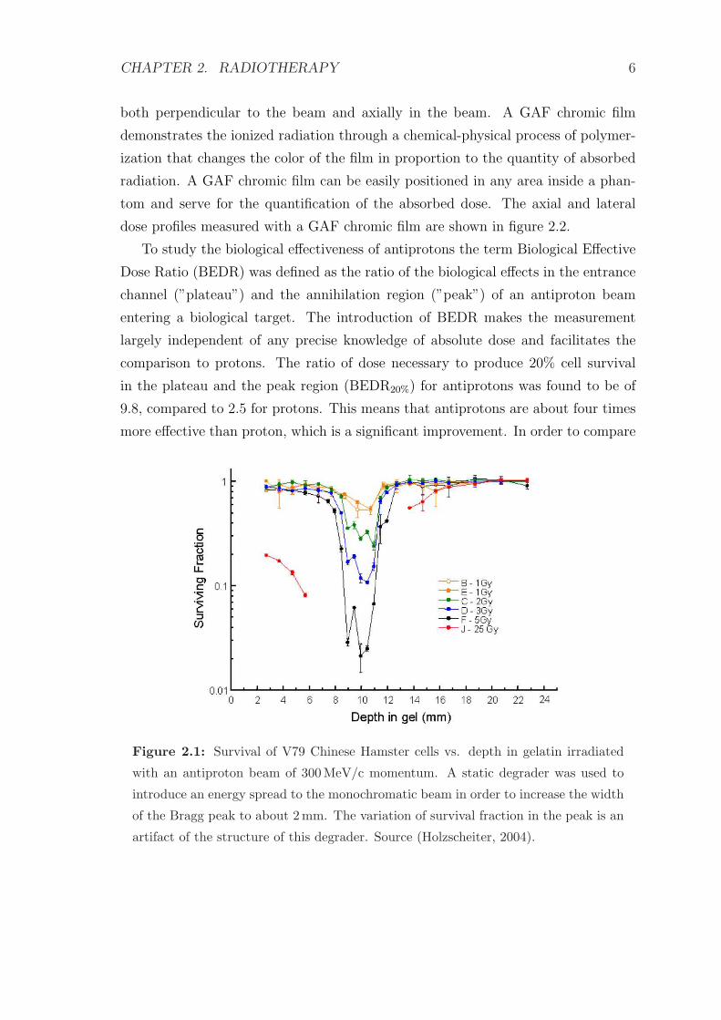
The tube was irradiated, then cut into 1mm slices along the beam axis and cell

survival fractions in each slice was determined. The whole experiment was repeated

for a variety of doses. A Bragg peak of mono-energetic beam of antiprotons is

only 1.5 mm wide at the FWHM value. The method of taking 1 mm thick samples

required the width of the peak to be enlarged. This was achieved with a static

degrader and the final width was 2.8mm. The fractions of survived cells in each

slice gave a family of survival vs. depth curves (Fig. 2.1).

Deposited energy was also measured by irradiating GAF chromic film placed

CHAPTER 2. RADIOTHERAPY 6

both perpendicular to the beam and axially in the beam. A GAF chromic film

demonstrates the ionized radiation through a chemical-physical process of polymer-

ization that changes the color of the film in proportion to the quantity of absorbed

radiation. A GAF chromic film can be easily positioned in any area inside a phan-

tom and serve for the quantification of the absorbed dose. The axial and lateral

dose profiles measured with a GAF chromic film are shown in figure 2.2.

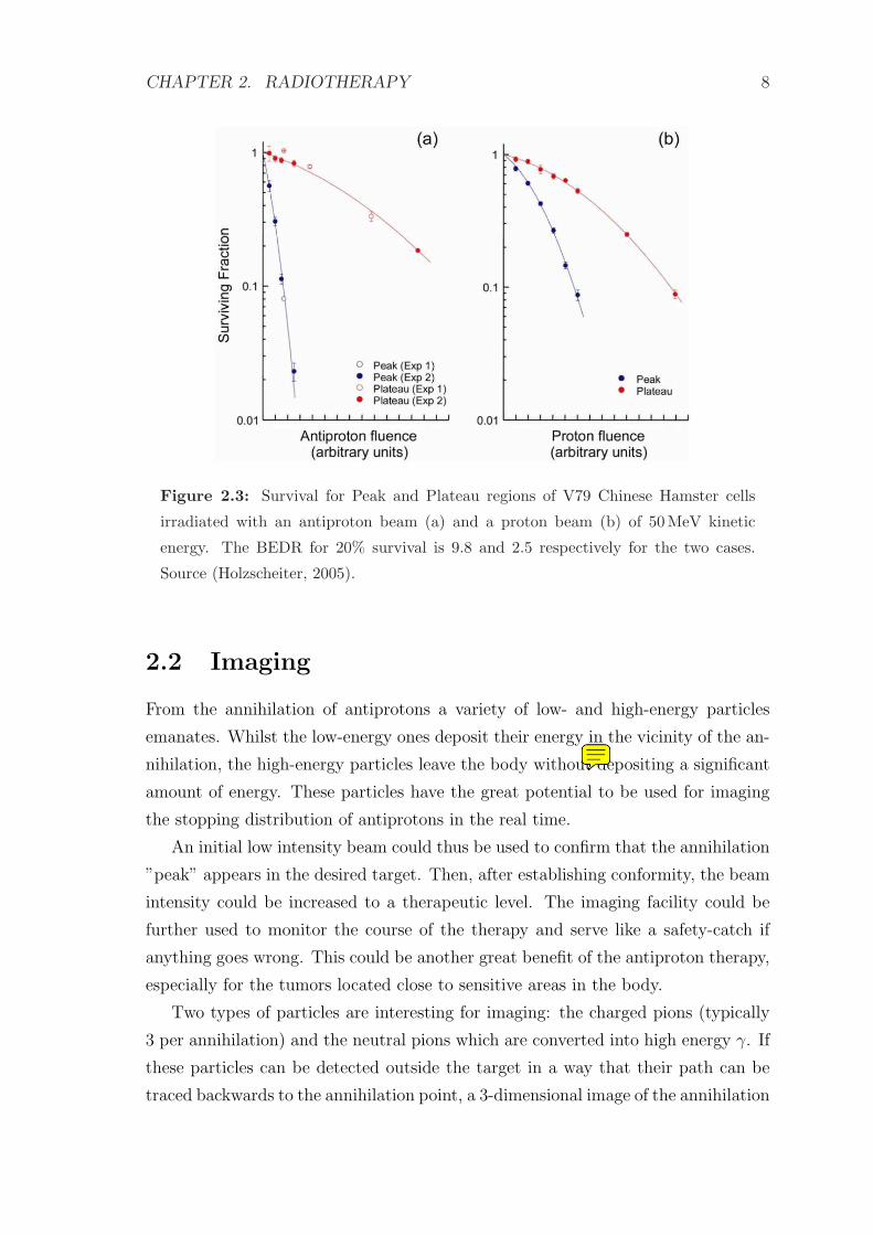
To study the biological effectiveness of antiprotons the term Biological Effective

Dose Ratio (BEDR) was defined as the ratio of the biological effects in the entrance

channel (”plateau”) and the annihilation region (”peak”) of an antiproton beam

entering a biological target. The introduction of BEDR makes the measurement

largely independent of any precise knowledge of absolute dose and facilitates the

comparison to protons. The ratio of dose necessary to produce 20% cell survival

in the plateau and the peak region (BEDR20%) for antiprotons was found to be of

9.8, compared to 2.5 for protons. This means that antiprotons are about four times

more effective than proton, which is a significant improvement. In order to compare

Figure 2.1: Survival of V79 Chinese Hamster cells vs. depth in gelatin irradiated

with an antiproton beam of 300MeV/c momentum. A static degrader was used to

introduce an energy spread to the monochromatic beam in order to increase the width

of the Bragg peak to about 2 mm. The variation of survival fraction in the peak is an

artifact of the structure of this degrader. Source (Holzscheiter, 2004).

CHAPTER 2. RADIOTHERAPY 7

Figure 2.2: (a) Axial and (b) radial profile of the dose deposited in a phantom as

measured with GAF chromic film. The lateral width of the beam was 3 cm, the width

of the Bragg peak 2.8 mm. Source (Agazaryan et al., 2003).

the data of proton and antiproton experiments, the position of plateau was redefined

for protons. It was defined as the slice which is at the same distance from the Bragg

peak as was used for the analysis of antiproton experiments. The summary of the

results is shown in Fig. 2.3.

In order to understand the significance of the results obtained with antiprotons

it is necessary to perform a direct comparison experiment with a beam of protons

and heavy ions under the same conditions as with the beam of antiprotons. For a

comparison with protons the TRIUMF facility in Canada was chosen. A first round

of comparison experiments conducted in 2003 and 2004 there and at CERN showed

a significant enhancement of the BEDR for antiprotons compared to protons. For

details see (appendix b of status report 2004). For a comparison experiment with

carbon ions the GSI facility in Darmstadt, Germany was chosen. This experiment

was approved for beam time in 2006 and 2007 and will be conducted in collaboration

with the biophysics group of Prof. G. Kraft at GSI.

CHAPTER 2. RADIOTHERAPY 8

Figure 2.3: Survival for Peak and Plateau regions of V79 Chinese Hamster cells

irradiated with an antiproton beam (a) and a proton beam (b) of 50 MeV kinetic

energy. The BEDR for 20% survival is 9.8 and 2.5 respectively for the two cases.

Source (Holzscheiter, 2005).

2.2 Imaging

From the annihilation of antiprotons a variety of low- and high-energy particles

emanates. Whilst the low-energy ones deposit their energy in the vicinity of the an-

nihilation, the high-energy particles leave the body without depositing a significant

amount of energy. These particles have the great potential to be used for imaging

the stopping distribution of antiprotons in the real time.

An initial low intensity beam could thus be used to confirm that the annihilation

”peak” appears in the desired target. Then, after establishing conformity, the beam

intensity could be increased to a therapeutic level. The imaging facility could be

further used to monitor the course of the therapy and serve like a safety-catch if

anything goes wrong. This could be another great benefit of the antiproton therapy,

especially for the tumors located close to sensitive areas in the body.

Two types of particles are interesting for imaging: the charged pions (typically

3 per annihilation) and the neutral pions which are converted into high energy γ. If

these particles can be detected outside the target in a way that their path can be

traced backwards to the annihilation point, a 3-dimensional image of the annihilation

CHAPTER 2. RADIOTHERAPY 9

volume can be obtained.

Although not mentioned in the original proposals the real-time imaging soon

became a solid part of the ACE experiment. A first prototype experiment designated

to test the possibilities of the real-time imaging was performed in November 2005

at AD at CERN by Michael Doser and Petra Riedler.

The analysis of this experiment forms one part of this thesis. The details of the

experiment are given, together with the analysis in the chapter 4. However at first

I will devote a short chapter to the physical principals of the beam therapy and to

the process of annihilation.

Chapter 3

Principles of beam therapy

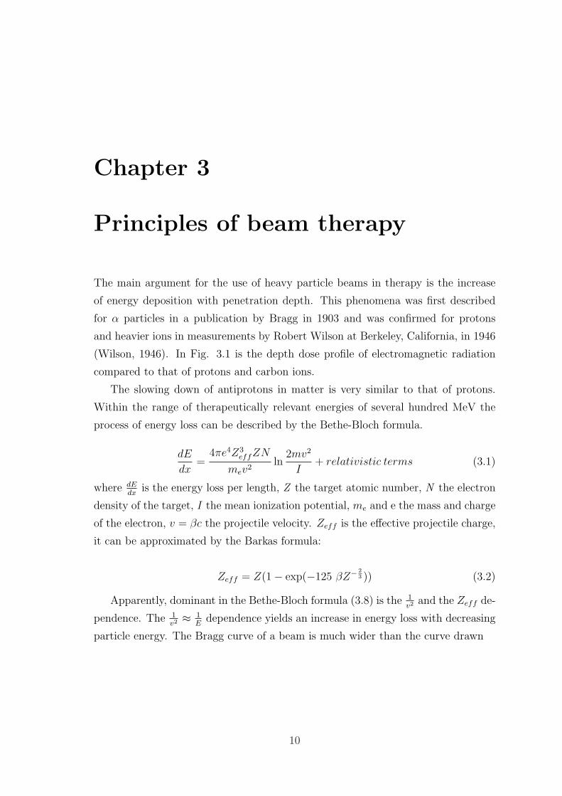
The main argument for the use of heavy particle beams in therapy is the increase

of energy deposition with penetration depth. This phenomena was first described

for α particles in a publication by Bragg in 1903 and was confirmed for protons

and heavier ions in measurements by Robert Wilson at Berkeley, California, in 1946

(Wilson, 1946). In Fig. 3.1 is the depth dose profile of electromagnetic radiation

compared to that of protons and carbon ions.

The slowing down of antiprotons in matter is very similar to that of protons.

Within the range of therapeutically relevant energies of several hundred MeV the

process of energy loss can be described by the Bethe-Bloch formula.

dE

dx=

4πe4Z3effZN

mev2ln

2mv2

I+ relativistic terms (3.1)

where dEdx

is the energy loss per length, Z the target atomic number, N the electron

density of the target, I the mean ionization potential, me and e the mass and charge

of the electron, v = βc the projectile velocity. Zeff is the effective projectile charge,

it can be approximated by the Barkas formula:

Zeff = Z(1− exp(−125 βZ− 23 )) (3.2)

Apparently, dominant in the Bethe-Bloch formula (3.8) is the 1v2 and the Zeff de-

pendence. The 1v2 ≈ 1

Edependence yields an increase in energy loss with decreasing

particle energy. The Bragg curve of a beam is much wider than the curve drawn

10

CHAPTER 3. PRINCIPLES OF BEAM THERAPY 11

Figure 3.1: Comparison of the depth dose profiles of electromagnetic radiation with

carbon ions and protons.

according to the Bethe-Bloch formula. This is caused by multiple scattering pro-

cesses. In reality it yields an almost Gaussian energy loss distribution f(∆E):

f(∆E) =1√2πσ

exp(∆E − 〈∆E〉)2

2σ2(3.3)

with

σ2 = 4πZ2effZN∆x

(1− β2

2

1− β2

)(3.4)

The width of the Bragg curve depends on the penetration depth ∆x of the

particles and thus the Bragg curve is wider for particles with greater energy. In

therapeutic praxis the active scanning is used to fill the target volume. If the Bragg

peak is too sharp too many slices are needed, and thus it can be advantageous to

widen the Bragg peak in order to decrease the overall treatment time. This is the

case especially for tumors that are located close to the surface.

CHAPTER 3. PRINCIPLES OF BEAM THERAPY 12

3.1 Lateral scattering

The lateral scattering of the therapeutic beam is at least as important as the depth

dose profile. In order to limit the risk, the treatment is always planned to avoid

the beam stopping in front of very sensitive regions. If the tumor is located close

to such a region the beam will pass by to the side. Here the knowledge of lateral

scattering is important when we decide how close the beam can get.

Lateral scattering mainly results from the Coulomb interaction of the projectile

with the target nuclei. In addition the kinematics of the nuclear reactions contributes

to the lateral width of a beam, predominantly at the distal side of the Bragg peak

where the primary projectiles are stopped and the residual dose is made up with

contributions of nuclear fragments only (Kraft, 2000). The angular distribution of

the scattering is again gaussian:

f(α) =1√

2πσα

exp

(− α2

2σα

)(3.5)

with

σα =14.1MeV

βpcZp

√d

Lrad

(1 +

1

9log10

d

Lrad

)(3.6)

where p is the momentum, Lrad the radiation length and d the thickness of the

material.

During the first ACE measurements in 2003 it was found that the damage to

samples placed outside the direct beam was minimal. Several approaches were used

to test this and the details can be found in (Holzscheiter, 2005).

3.2 Conformal beam treatment

The increased dose and high biological efficiency at the end of the particle range can

only be fully exploited with a so called target-conformal treatment. In very modern

facilities for ion beam therapy such as PSI in Villingen and GSI in Darmstadt

the dose is conformed to the tumour by lateral beam scanning. In this treatment

technique, the target volume is divided into slices of equal particle range and each

slice is treated by scanning the beam laterally over each slice. The slice to be treated

is covered by a net of pixels that have to be filled by a definite but varying particle

fluence according to the dose necessary to produce a homogeneous dose or biological

effect.

CHAPTER 3. PRINCIPLES OF BEAM THERAPY 13

Weber et al. (Weber et al., 2000) have recently proposed an alternative scanning

method with a intensity-controlled longitudinal scan in the beam direction, called

”depth scanning”. This method yields the same conformity as a lateral scan system

but requires a less expensive construction and control system. For depth scanning

the target volume is divided into cylinders with the central axis parallel to the beam

axis. Then the fast longitudinal scanning is applied in a series of such cylinders. It

means that the Bragg maximum is continuously shifted along the central axis of the

cylinder with a velocity up to 50 cm·s−1.

In order to exploit the advantages of antiprotons in radiotherapy one of the

described or a similar system should be applied in practise.

3.3 Annihilation

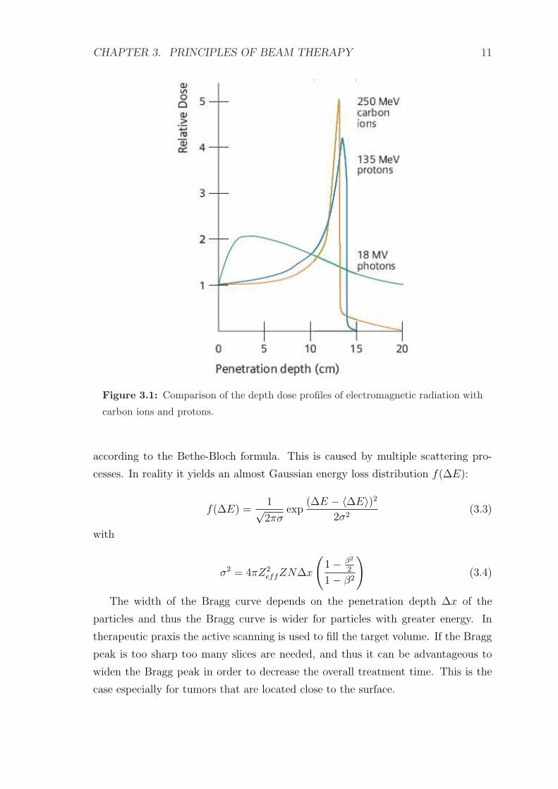
The antiproton nucleon annihilation occurs at rest or at low energies. The figures

3.2, 3.3 show pp and pn cross sections respectively. Annihilation is a process in

which the baryons undergo a transition into mesons. The transition is viewed in

the quark model basically as a rearrangement of all incoming quarks and antiquarks

into quark-antiquark pairs. However the process in which some of the quarks and

antiquarks annihilate and new quark-antiquark pairs are produced is also frequent.

This makes the theoretical description particulary difficult.

During the annihilation event mostly pions are produced.

Figure 3.2: Total and elastic cross sections for pp collision as a function of laboratory

beam momentum and total center-of-mass energy. Source (Eidelman et al., 2004).

CHAPTER 3. PRINCIPLES OF BEAM THERAPY 14

Figure 3.3: Total and elastic cross sections for pd (total only) and pn collisions as

a function of laboratory beam momentum and total center-of-mass energy. Source

(Eidelman et al., 2004).

The average pion multiplicity for the pp annihilation is estimated to:

nπ = 4.98± 0.13, nπ± = 3.05± 0.04, nπ0 = 1.93± 0.12 (3.7)

The fraction of purely neutral annihilations (mainly from channels like 3π0, 5π0,

2π0η, and 4π0η decaying to photons only) is (3.56±0.3)%. In addition to pions, η

mesons are produced with a rate of about 7% and kaons with a rate of about 6% of

all annihilations (Klempt et al., 2005), (Amsler, 1998).

The most detailed experiments to study the annihilation were performed at the

LEAR facility at CERN, KEK facility in Japan and in Brookhaven National Labo-

ratory. For review see e.g. (Amsler and Myhrer, 1991), (Amsler, 1998) and (Klempt

et al., 2005). In most of the experiments antiprotons were stopped in liquid or

gaseous H2 or D2 and thus the majority of the data can be found for hydrogen.

The detailed survey of the annihilation mechanism is beyond the scope of this thesis

and can be found elsewhere, e.g. (Klempt et al., 2005). I will give only a general

review of the known facts and emphasize the details that are most important for

the purposes of the imaging.

An antiproton stopping in hydrogen is captured to form an antiprotonic hydrogen

atom. The highest probability of forming the pp system is for high principal quantum

numbers: n∼ 30. The binding energy of the system corresponds to the binding

energy of the electron ejected during the capture process. The deexcitation proceeds

CHAPTER 3. PRINCIPLES OF BEAM THERAPY 15

via two different mechanisms. (a) Stark mixing, which dominates in liquid hydrogen

and (b) the cascade to lower levels by x-ray or external Auger emission of electrons

from neighboring molecules, which takes place mostly for the gaseous hydrogen.

In the liquid hydrogen collisions between the pp atom and neighboring molecules

induce transitions from high angular momentum states, the process called Stark

mixing. Thus the protonium annihilates with the angular momentum ` = 0, from

high S levels (S-wave annihilation). The initial states are spin singlets 1S0 and spin

triplets 3S1.

In the gaseous medium the annihilation collision frequency is much lower and the

annhilation occurs mainly with the angular momentum ` = 1 (P-wave annihilation).

Details of the S-wave and P-wave annihilations can be found e.g. in (Klempt et al.,

2005). Annihilation from states with ` ≥ 2 can be ignored due to the negligible

overlap of p and p in the atomic wavefunction. The branching ratio between the S-

wave and P-wave annihilation depends on the density of the target. The dependance

of the P-wave fraction on the density shows the figure 3.4.

Figure 3.4: Fraction of P-wave annihilation as a function of hydrogen density (curve).

The dots with error bars give the results from the optical model of Dover and Richard

(1980) using two-body branching ratios. Source (Amsler, 1998).

The unified theory for the pion spectrum calculation was presented by Amado

et al. in 1994 (Amado et al., 1994). In their picture the annihilation at rest is

very rapid and results in a pion wave radiated from the annihilation vertex. The

CHAPTER 3. PRINCIPLES OF BEAM THERAPY 16

pion wave is subsequently quantized using the method of coherent states (Horn and

Silver, 1970). Applying the constraints of isospin and four-momentum conservation

leads to the pion spectrum given in the Fig. 3.5. The results are in a very good

agreement with experiments.

Figure 3.5: The probability, Pm, of having m pions in nucleon-antinucleon annihila-

tion at rest as a function of m. The open circles refer to unconstrained coherent state

and form a Poisson distribution. The solid squares include the constraint of four-

momentum conservation and form the Gaussian distribution that agrees well with the

experiment. Source (Amado et al., 1994).

3.4 Monte Carlo Simulation

For the simulation of the experiment we chose the Monte Carlo program GEANT4

(Agostinelli et al., 2003). GEANT4 is a toolkit for simulating the passage of particles

through matter. It includes tools for designing the geometry of the system, the large

set of materials and fundamental particles and most importantly, a wide range of

physical processes. This enable us to generate a primary particle, to track its passage

through the defined geometry and to record its interaction with the materials and

the response of sensitive detectors.

In GEANT4 the mean energy loss of the antiprotons is calculated according to

the restricted Bethe-Bloch formula:

dE

dx= KNel

Z2eff

β2

(ln

2 mec2β2γ2Tmax

I2− β2(1 +

Tc

Tmax

)− 2 Ce

Z

)(3.8)

CHAPTER 3. PRINCIPLES OF BEAM THERAPY 17

where Nel is the electron density of the medium, Tmax the maximum energy trans-

ferable to the free electron, Tc the threshold energy above which the δ-rays are

generated and Ce/Z is the shell correction term. The concrete values of the correc-

tion terms can be found in the GEANT4 documentation (Agostinelli et al., 2003).

The accuracy of this formula is estimated as 1%.

The antiproton-nucleon reactions are implemented in GEANT4 with the quark

level chiral invariant phase space (CHIPS) model. The antinucleon-nucleon anni-

hilation algorithm is explained in detail (Degtyarenko et al., 2000). The first step

of the CHIPS algorithm is the annihilation of antiprotons on peripheral nucleons,

followed by the creation of an internuclear hadronic excitation (quasmons). The

quasmon dissipates its energy and produces secondary nuclear fragments. The spec-

tra of pions and nuclear fragments generated with the CHIPS model are in a very

good agreement with the experimental data. The details of the CHIPS performance

in antiproton-nuclear annihilation can be found in (Kossov, 2005).

In the simulation I use the G4QCaptureAtRest process for all negative hadrons

Figure 3.6: Energy deposition of an antiproton stopping in glycerin. The graph

shows contributions of individual products of annihilation and inelastic collisions;

namely of protons, deuterons, tritons, alpha particles, 3He, and heavier fragments as

a function of a penetration depth.

CHAPTER 3. PRINCIPLES OF BEAM THERAPY 18

in GEANT4 Physics List. This applies the CHIPS algorithm for all capture at

rest processes. Figure 3.6 shows the details for the energy deposition of antiprotons

annihilating in glycerin. It shows the individual contributions of protons, deuterons,

tritons, alpha particles, 3He, and other (heavier) secondaries as a function of a

penetration depth. A large fraction of annihilation products have a small momentum

in the beam direction and thus are not emitted completely isotropically in space.

Figures 3.7 and 3.8 show the momentum spectra of particles emanating from the

annihilation vertex in the GEANT4 simulation.

0 200 400 600 800 10000.0

0.2

0.4

0.6

0.8

1.0

+

coun

ts [a

rb.u

nits

](n

orm

aliz

ed to

1)

p [MeV/c]

0 200 400 600 800 10000.0

0.2

0.4

0.6

0.8

1.0

coun

ts [a

rb.u

nits

](n

orm

aliz

ed to

1)

p [MeV/c]

Figure 3.7: Momentum spectra of the particles created during simulated annihilation

in Geant4. The upper panel shows spectrum of π+, the lower of π−.

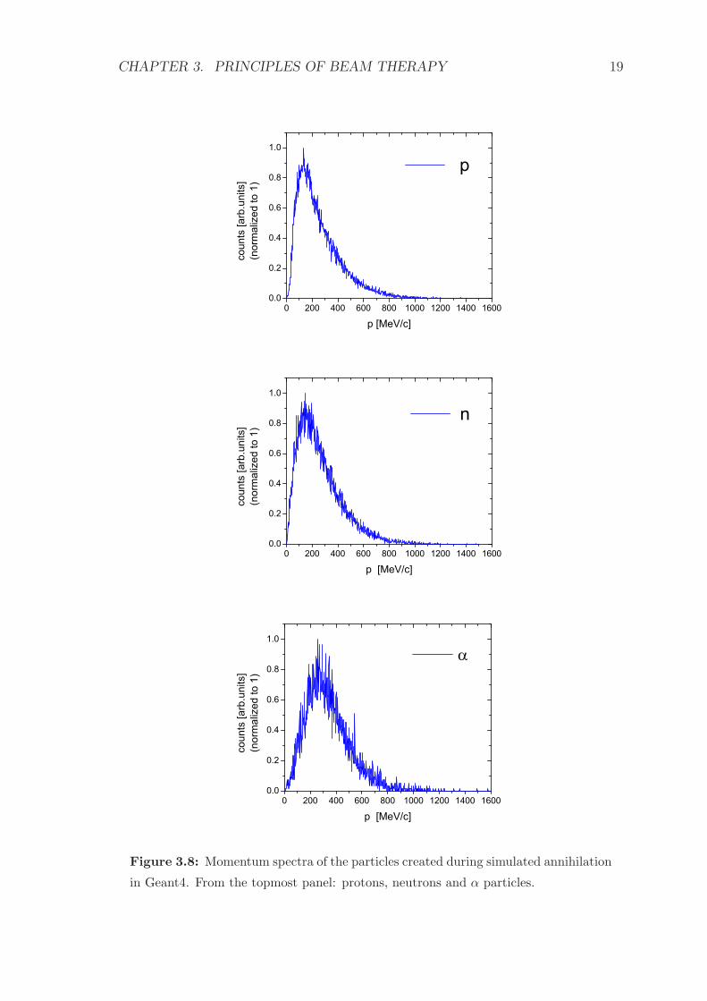
CHAPTER 3. PRINCIPLES OF BEAM THERAPY 19

0 200 400 600 800 1000 1200 1400 16000.0

0.2

0.4

0.6

0.8

1.0

p

coun

ts [a

rb.u

nits

](n

orm

aliz

ed to

1)

p [MeV/c]

0 200 400 600 800 1000 1200 1400 16000.0

0.2

0.4

0.6

0.8

1.0

n

coun

ts [a

rb.u

nits

](n

orm

aliz

ed to

1)

p [MeV/c]

0 200 400 600 800 1000 1200 1400 16000.0

0.2

0.4

0.6

0.8

1.0

coun

ts [a

rb.u

nits

](n

orm

aliz

ed to

1)

p [MeV/c]

Figure 3.8: Momentum spectra of the particles created during simulated annihilation

in Geant4. From the topmost panel: protons, neutrons and α particles.

Chapter 4

The Prototype Experiment and its

Analysis

The experiment that for the first time directly tested whether the pions emanating

from the annihilation vertex could be used in the real-time imaging was performed

in November 2005 at CERN by Michael Doser and Petra Riedler. The beam of

antiprotons was extracted from the Antiproton Decelerator (AD).

Figure 4.1: The scheme of PS experiments including the AD ring.

The AD is a facility which produces a low-energy beam of antiprotons. A pro-

ton beam at 26 GeV/c is extracted from PS (Proton Synchrotron) and delivered

onto a Copper or Iridium target. Of 1.5×1013 protons about 5×107 antiprotons at

3.57GeV/c are created and then the beam is decelerated. The deceleration proceeds

20

CHAPTER 4. THE PROTOTYPE EXPERIMENT AND ITS ANALYSIS 21

in several consecutive steps (Fig. 4.2) and takes 100 s. At first stochastic cooling is

applied and the beam is decelerated down to 2GeV/c. Afterwards electron cooling

slows the beam down to 100MeV/c. At the end 3×107 antiprotons are available at

low energy for the experiments. The detailed information about AD can be found

in e.g. (Belochitskii et al., 2004).

Figure 4.2: AD cycle.

For the ACE experiment a pulse of 3×107 antiprotons with p = 300 MeV was

extracted from the AD was sent onto a water target (a cylinder of a radius 2.5 cm

and length 20 cm). The antiprotons stopped simultaneously in the water. The

stopping distribution is expected to have the form of a sigmoid, with a width of

3 cm transverse to the beam axis, and 2mm along the beam axis. The charged

pions were emitted isotropically and a fraction of them was detected. A scheme of

the setup used is sketched in the Fig. 4.3.

A standard multiplane silicon pixel detector was chosen to detect charged pions.

Particulary a prototype of the ALICE chip, developed at CERN was used. The

ALICE1LHCB Pixel chip contains 8192 pixel cells, each with a size of 50× 425µm2.

The cells are arranged in a matrix with 32 columns and 256 rows. The sensor

thickness is 300µm and the chip thickness 725µm. Three such pixel chips were

placed 193 cm far from the water target, aligned as is shown in the Fig. 4.3.

CHAPTER 4. THE PROTOTYPE EXPERIMENT AND ITS ANALYSIS 22

p

193 cm

13.2 cm

2 cm

AD

100 cm

ALICE pixel

detectors

water target

z

x

2 cm

origin of the

coordinate system

Figure 4.3: The experimental setup used in the first experiment to test the imaging

potential, performed at the AD at CERN in November 2004. The figure shows the

setup in a top view.

The aim of the experiment was to show that the tracks of detected pions can be

reconstructed and the parameters of the stopping distribution gained. Unfortunately

we cannot expect any correlation among the registered pions, because it is very

unlikely that any given pair would come from the same annihilation vertex. This

makes the reconstruction of the parameters particulary difficult.

I address the analysis of this experiment in the next section. I present there a

GEANT simulation of the experiment and an algorithm developed for a reconstruc-

tion of the stopping distribution parameters. The algorithm is applied on experi-

mental and simulated data. Limitations of the current setup are clear and therefore

I propose an improved experimental setup for the next experiments. This proposal

is described in the next chapter.

4.1 GEANT4 simulation

I have simulated the experiment using the Monte Carlo package GEANT4, shortly

described in the section 3.4. For a schematic top view of the setup see Fig. 4.3. The

origin of the coordinate system was located on the beam axis, 2 cm deep in the water

target, as is shown in the figure. The y axis points out of the figure. The antiprotons

with energy 300± 0.1MeV came from the source located at z = −1.02m, i.e. 1m

away from the water target. The distribution of the beam transverse to the beam

axis was Gaussian with the width of 3 cm. The water target was surrounded by

air under standard conditions. The set of the the three silicon pixel detectors was

CHAPTER 4. THE PROTOTYPE EXPERIMENT AND ITS ANALYSIS 23

rotated 45 degrees about the y axis, facing the volume where most of the annihilation

events were expected to take place. For the detector location see the scheme.

In order to decrease the overall run time of the simulation I used detectors 100

times larger, i.e. 10× 10 ALICE chips described above. Thus each of the detectors

had 2560 rows and 320 columns. The width of the chips was 300 µm.

The detectors as well as the water target was set sensitive and the coordinate of

each pixel receiving a hit was registered. The exact coordinate of the annihilation

vertex was saved only when a product of this annihilation event hit the detectors.

A preview of a typical event generated with GEANT4 is in the Fig. 4.4.

Figure 4.4: A top view on the GEANT4 simulation of an antiproton stopping in

a water target. The red horizontal red line on the left side shows a p coming from

the source, the turquoise rectangle is the water target. Colors of the lines correspond

to the charge of the particle: red – negative, blue – positive and green neutral. The

majority of the green lines are γ.

4.2 Algorithm for the experiment analysis

An algorithm for the reconstruction of the stopping distribution analysis has been

developed. The reconstruction is not very precise with the experimental design

described above but the ideas can be used in the improved experimental design

that is suggested in the next chapter. Through the whole document the system of

coordinates introduced in the figure 4.3 is used. The origin of the system is located

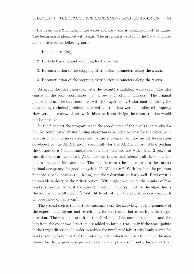
CHAPTER 4. THE PROTOTYPE EXPERIMENT AND ITS ANALYSIS 24

at the beam axis, 2 cm deep in the water and the y axis is pointing out of the figure.

The beam axis is identified with z axis. The program is written in the C++ language

and consists of the following parts:

1. Input file reading.

2. Particle tracking and searching for the z-peak.

3. Reconstruction of the stopping distribution parameters along the x axis.

4. Reconstruction of the stopping distribution parameters along the y axis.

As input the files generated with the Geant4 simulation were used. The files

consist of the pixel coordinates, i.e. a row and column numbers. The original

plan was to use the data measured with the experiment. Unfortunately during the

data taking technical problems occurred and the data were not collected properly.

However as it is shown later, with this experiment design the reconstruction would

not be possible.

In the first part the program reads the coordinates of the pixels that received a

hit. No complicated cluster finding algorithm is included because for the experiment

analysis it will be more convenient to use a program for precise hit localization

developed by the ALICE group specifically for the ALICE chips. While reading

the output of a Geant4 simulation only hits that are not wider than 2 pixels in

each direction are validated. Also, only the tracks that intersect all three detector

planes are taken into account. The first detector (the one closest to the target)

optimal occupancy, for good analysis is 25 - 35 hits/cm2. With less hits the program

finds the z-peak location (± 1.5mm) and the y distribution fairly well. However it is

impossible to describe the x distribution. With higher occupancy the number of fake

tracks is too high to trust the algorithm output. The top limit for the algorithm is

the occupancy of 50 hits/cm2. With little adjustment the algorithm can work with

an occupancy of 3 hits/cm2.

The second step is the particle tracking. I use the knowledge of the geometry of

the experimental layout and search only for the tracks that come from the target

direction. The reading starts from the third plane (the most distant one) and the

hits from the other two detectors are added to form a track only if the track points

in the target direction. In order to reduce the number of fake tracks I only search for

tracks coming from a part of the water cylinder, which is chosen to include the area

where the Bragg peak is expected to be located plus a sufficiently large area that

CHAPTER 4. THE PROTOTYPE EXPERIMENT AND ITS ANALYSIS 25

surrounds it. For example, when I searched for the Bragg peak which was expected

to be 2 cm deep in the target I assumed that it would be not deeper than 4 cm.

I perform different tracking for the analysis in each direction. While searching

the z-peak, the sharp peak in the depth dose profile I make the following assumption:

only a negligible fraction of annihilations occur deeper than 4 cm and the stopping

distribution does not depend on y. I search the tracks coming from a narrow slice

x ∈ (−25, 25)mm, y ∈ (−2, 2)mm.

If the occupancy of the detectors is not too high (see above) I find approximately

the right number of tracks. It is very unlikely that any pair of tracks come from

the same annihilation vertex. An intersection of each of the tracks with the target

volume is a line segment, up to few centimeters long. There is no way how to

determine where exactly on this segment the annihilation occurred.

To determine the location of the z-peak I use the fact that the distribution

transverse to the beam axis is regular. It means that there is approximately the

same number of particles coming from the x > 0 half of the water target as from the

x < 0 half. Thus the central line of the bunch of the reconstructed tracks intersects

the central beam line (z axis) at the point where the z-peak is located. The central

line is found so that intersections of all the tracks with two arbitrary planes, parallel

to the detectors are found. In each of these planes a central point is calculated

according to:

~R =

n∑i=1

~ri

n(4.1)

where ~ri correspond to the intersections and n is the number of tracks. The central

line is obtained with connecting these two points.

The main problem for the precise reconstruction is the finite width of the pixel

(0.425mm), which hinders accurate track reconstruction. The error on the z axis

for a single track can be in the worst case 15mm. However, if the statistics is high

enough these errors cancel and the error for the central line is reduced to 2 mm.

The reconstruction along the y axis gives the best results, because of two reasons:

1) the detector resolution in the vertical direction is 8.5 times better than in the hor-

izontal, 2) the detectors are not rotated about the z axis and thus the reconstructed

tracks include the plane y = 0 only at a small angle. Hence the error in estimate of

the y coordinate of the annihilation is much smaller. To reconstruct the distribution

I use a method which I later on refer to as a scanning method. I calculate how many

CHAPTER 4. THE PROTOTYPE EXPERIMENT AND ITS ANALYSIS 26

occupancy (hits/cm2) depth of z-peak (mm) σy (mm)

3 18.4 23.5 ± 7.4

6 17.4 24.8 ± 6.7

17 17.3 27.2 ± 6.3

25 18.3 18.3 ± 1.9

30 18.9 17.8 ± 1.7

35 18.8 19.6 ± 1.8

50 19.3 19.1 ± 2.4

Table 4.1: Reconstruction of the simulated experiment. The occupancy is given

for the the 1st detector plane (the plane which is closest to the target), σy is a half

width of a gaussian fit to the found distribution. The real parameters were: depth of

z-peak = 18.4mm, σy = 17 mm.

tracks come from the slices y ∈ (yc, yc + 2) mm and y ∈ {−25,−23, .., 23}mm, i.e.

the program scans the target volume along the y axis and counts the number of

tracks in each of the scanned part. The results obtained are plotted and compared

to the simulation output in the Figure 4.6.

10 12 14 16 18 20 220.0

0.2

0.4

0.6

0.8

1.0

Num

ber o

f ann

ihila

tion

even

ts(n

orm

aliz

ed to

1)

Penetration depth [mm]

Figure 4.5: Stopping distribution of antiprotons in water as a function of penetration

depth, simulated with Geant4.

CHAPTER 4. THE PROTOTYPE EXPERIMENT AND ITS ANALYSIS 27

In Table 4.1 the results found with the algorithm for the samples of different

occupancies are summarized and σy comes from a gaussian fit. In the Geant4 simu-

lation the stopping distribution was a sigmoid with a width of 34mm transverse to

the beam axis and 3mm along the beam axis. The z-peak was located at the depth

of 18.6mm. The profile of the peak calculated with Geant4 is shown in the Fig. 4.5.

The tracking for the x axis analysis is performed for a volume of x ∈ (−25, 25)mm,

y ∈ (−2, 2)mm and z ∈ (z-peak − 10, z-peak + 10)mm. Intersections of the tracks

found with a plane z = z-peak are found. The projection of the intersections to the

x axis yields the distribution in the x direction. The results obtained are plotted

and compared to the simulation output in the Figure 4.6.

CHAPTER 4. THE PROTOTYPE EXPERIMENT AND ITS ANALYSIS 28

-30 -20 -10 0 10 20 300.0

0.2

0.4

0.6

0.8

1.0

Num

ber o

f ann

ihila

tion

even

ts (

norm

aliz

ed to

1)

x (mm)

-30 -20 -10 0 10 20 300.0

0.2

0.4

0.6

0.8

1.0

Num

ber o

f ann

ihila

tion

even

ts(n

orm

aliz

ed to

1)

y (mm)

Figure 4.6: Stopping distribution of antiprotons in water along the x (upper panel)

and y (lower panel) axis. The black squares show the output of Geant4 simulation,

blue open circles the reconstruction performed with the algorithm described above.

The occupancy of the 1st detector was 30 hits/cm2.

CHAPTER 4. THE PROTOTYPE EXPERIMENT AND ITS ANALYSIS 29

4.3 Conclusion

Apparently the reconstruction is not very accurate. The distribution in the x direc-

tion is not reconstructed precisely. In the z direction it is only possible to determine

an approximative position of the peak. The reconstruction precision is probably

sufficient for therapeutic purposes.

I do not think that there is a way to significantly improve the algorithm. The

reasons for the inaccuracy lie in the design of the experiment. As was mentioned be-

fore, even when the right track is reconstructed it is not possible to determine where

exactly on the intersection of the track with the target the annihilation occurred.

Putting some assumptions on the symmetry of the layout it is possible to estimate

where the z-peak was located but i didn’t find a way to reasonably estimate the

width of the peak.

Making the intersection of all the tracks with the plane z = z-peak, i.e. with the

plane where the majority of annihilations occurred a rough estimate of the x axis

distribution can be made. However it is not possible to select the tracks that belong

to the annihilation events which took place in this plane and the distribution is

blurred. The best estimate I got is shown in the Figure 4.6.

The other problem is, that the analysis was performed on 100 times larger de-

tectors. The original experiment was carried out with detectors of surface equal

174.08mm2 and when I assume that the annihilation products were emitted as they

are emitted in Geant4 it received about 330 hits. With the occupancy of 190 hits/cm2

the algorithm would not work anyway.

Significantly improved results can be obtained with rather small changes in the

experimental setup. Such changes are described in the next chapter.

Chapter 5

Proposal For The Next

Experiment

A clear conclusion of the last chapter is that a single set of detectors is not sufficient

for a good three dimensional reconstruction of the stopping distribution. Another

important observation is that the scanning method (the method used in the previous

chapter for the reconstruction along the y axis) proved to be successful for the

detector situated parallel to the axis of interest (in that case the y axis).

The aim was to improve the reconstruction with as few added detectors as possi-

ble. I propose two different layouts and describe their advantages and disadvantages.

The simulations were written again in GEANT4, the program for the reconstruction

is described in detail in the Appendix.

In simulations a different target was used than in the original experiment. Here I

used a cube of water with an edge length of 10 cm. The reasons for the change was to

approximate a prospective medical target, in this case the head. This approximation

is important because the pixel detectors detect all charged particles, not only the

pions coming directly from the annihilation vertex. The annihilation products, after

emanating from the annihilation vertex collide further. Products of these collisions

also reach the detectors and blur the distribution of pions. The number of these

particles depend on the distance that the annihilation products travel in the water,

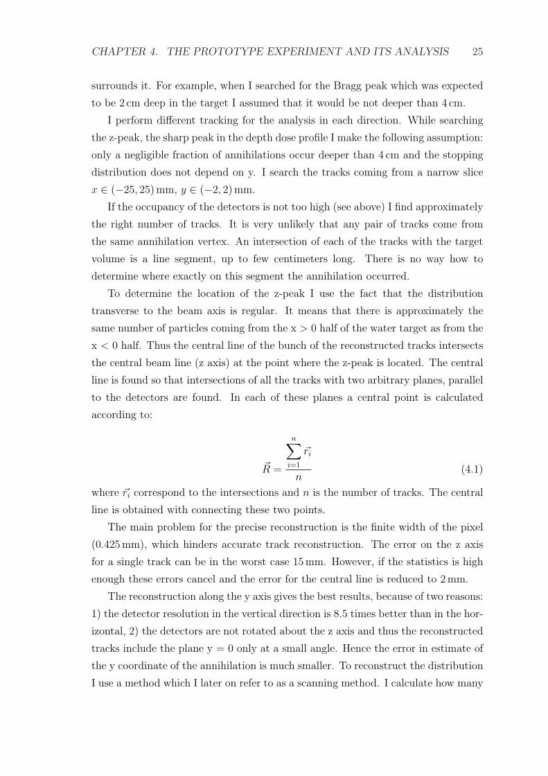
namely on the size of the target. The table 5.1 shows the number of hits generated

by various particles in the detectors situated behind and parallel to the target. Two

different target sizes are presented: a cube with edge length equal to 10 cm and

20 cm.

The most problematic particles are e− and e+ which are either delta electrons or

stem from pair production. In both cases they do not come from the annihilation

30

CHAPTER 5. PROPOSAL FOR THE NEXT EXPERIMENT 31

particle Hits [%] Hits [%]

target edge = 10 cm target edge = 20 cm

Parallel Perpendicular Parallel Perpendicular

π− 19.4 29 16.7 24.8

π+ 16.6 19.6 14.7 15.6

e− 31.5 24.9 38.4 35.1

e+ 9.2 9.7 14.9 15.1

p 14.1 12.5 8.8 6.3

d 1.7 0.8 0.5 0.1

µ− 4.2 1.8 3.3 1.6

µ+ 3.2 1.7 2.6 0.9

Table 5.1: The percentage of hits generated by various particles in the detector

parallel and perpendicular to the beam axis. As a target was used in both cases a

cube of water. The first column shows the results for the cube of the edge length equal

10 cm, the second column of the edge length equal 20 cm. The width of the beam at

FWHM was 3 cm.

vertex, which makes them particulary problematic. On the other hand they mostly

do not have very high energies and thus scatter easily. The hits that they leave

in detectors often do not cross the detectors on a straight trajectory and therefore

are not included in the bunch of reconstructed tracks. Although there are less of

them in the perpendicular detector, they have higher energies, which makes the

reconstruction from these detectors less precise.

There are also a significant amount of protons hitting the detectors. They are

emitted during the nucleus fragmentation following the annihilation process. A

spectrum of these protons is given in figure 3.8. The protons mostly come from

the annihilation vertex, but often do not have sufficient energy to leave a straight

track in the detectors. From the table 5.1 it follows that if the passage from the

annihilation vertex through the target is longer far less protons reach the detectors.

The number of registered electrons slightly increases with the target size.

5.1 A layout using two detector sets

The first proposed design consists of two sets of detectors instead of one. One of them

is designated to recognize the depth dose profile and the other one to reconstruct

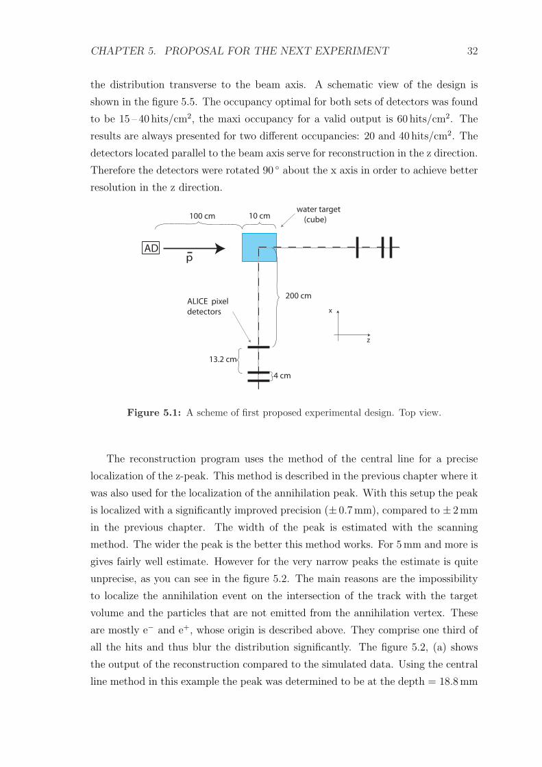
CHAPTER 5. PROPOSAL FOR THE NEXT EXPERIMENT 32

the distribution transverse to the beam axis. A schematic view of the design is

shown in the figure 5.5. The occupancy optimal for both sets of detectors was found

to be 15 – 40 hits/cm2, the maxi occupancy for a valid output is 60 hits/cm2. The

results are always presented for two different occupancies: 20 and 40 hits/cm2. The

detectors located parallel to the beam axis serve for reconstruction in the z direction.

Therefore the detectors were rotated 90 ◦ about the x axis in order to achieve better

resolution in the z direction.

p

13.2 cm

4 cm

AD

100 cm

ALICE pixel

detectors

water target

(cube)

z

x

10 cm

200 cm

Figure 5.1: A scheme of first proposed experimental design. Top view.

The reconstruction program uses the method of the central line for a precise

localization of the z-peak. This method is described in the previous chapter where it

was also used for the localization of the annihilation peak. With this setup the peak

is localized with a significantly improved precision (± 0.7mm), compared to ± 2mm

in the previous chapter. The width of the peak is estimated with the scanning

method. The wider the peak is the better this method works. For 5mm and more is

gives fairly well estimate. However for the very narrow peaks the estimate is quite

unprecise, as you can see in the figure 5.2. The main reasons are the impossibility

to localize the annihilation event on the intersection of the track with the target

volume and the particles that are not emitted from the annihilation vertex. These

are mostly e− and e+, whose origin is described above. They comprise one third of

all the hits and thus blur the distribution significantly. The figure 5.2, (a) shows

the output of the reconstruction compared to the simulated data. Using the central

line method in this example the peak was determined to be at the depth = 18.8 mm

CHAPTER 5. PROPOSAL FOR THE NEXT EXPERIMENT 33

when the occupancy was 20 hits/cm2 and 18.1mm when 40 hits/cm2. Geant4 output

peak was at 18.5mm.

It should be kept in mind that in medical applications the Bragg peak will

be perhaps enlarged in order to reduce the overall treatment time. In the lateral

scanning method, described in the section 3.2 a typical width of the slice is 4-5mm,

which corresponds to the width (FWHM) of the Bragg peak. In the depth scanning

method the width of the Bragg peak corresponds to the width of the tumor (up to

few cm). It is therefore necessary that the imaging method recognizes the wider

peaks well. I made simulations with 2 different spread-out Bragg peaks, one with a

width of 5mm and the second one with a width of approximately 1 cm. Results of

the reconstruction for these peaks are shown in figure 5.3.

0 5 10 15 20 25 30 35 40 45 50

0.0

0.2

0.4

0.6

0.8

1.0 GEANT4 output 20 hits/cm2

40 hits/cm2

Num

ber o

f ann

ihila

tion

even

ts (

norm

aliz

ed to

1)

Penetration depth (mm)

(a)

Figure 5.2: Stopping distribution of monoenergetic antiprotons in a water target

along the beam axis. The black lines show output of Geant4 simulation, the result of

the reconstruction is shown for the occupancy of 20 hits/cm2 (blue open circles) and

40 hits/cm2 (green triangles).

CHAPTER 5. PROPOSAL FOR THE NEXT EXPERIMENT 34

0 5 10 15 20 25 30 35

0.0

0.2

0.4

0.6

0.8

1.0 Geant4 20 hits/cm2

40 hits/cm2

Num

ber o

f ann

ihila

tion

even

ts(n

orm

aliz

ed to

1)

Penetration depth [mm]

(a)

0 5 10 15 20 25 30 35

0.0

0.2

0.4

0.6

0.8

1.0 Geant4 20 hits/cm2

40 hits/cm2

Num

ber o

f ann

ihila

tion

even

ts(n

orm

aliz

ed to

1)

Penetration depth [mm]

(b)

Figure 5.3: Stopping distribution of antiprotons in a water target along the beam

axis for two different spread-out Bragg peaks. The black lines show output of Geant4

simulation, the result of the reconstruction is shown for the occupancy of 20 hits/cm2

(blue open circles) and 40 hits/cm2 (green triangles).

CHAPTER 5. PROPOSAL FOR THE NEXT EXPERIMENT 35

-60 -40 -20 0 20 40 60

0.0

0.2

0.4

0.6

0.8

1.0 GEANT4 output 20 hits/cm2

40 hits/cm2

Num

ber o

f ann

ihila

tion

even

ts(n

orm

aliz

ed to

1)

x [mm]

-60 -40 -20 0 20 40 60

0.0

0.2

0.4

0.6

0.8

1.0

GEANT4 output 20 hits/cm2

40 hits/cm2

Num

ber o

f ann

ihila

tion

even

ts(n

orm

aliz

ed to

1)

y [mm]

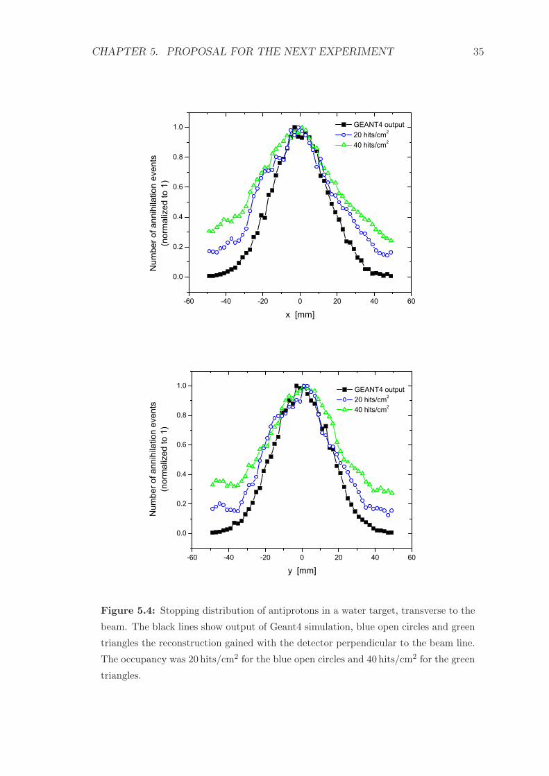
Figure 5.4: Stopping distribution of antiprotons in a water target, transverse to the

beam. The black lines show output of Geant4 simulation, blue open circles and green

triangles the reconstruction gained with the detector perpendicular to the beam line.

The occupancy was 20 hits/cm2 for the blue open circles and 40 hits/cm2 for the green

triangles.

CHAPTER 5. PROPOSAL FOR THE NEXT EXPERIMENT 36

The detector set perpendicular to the beam axis, placed behind the target serves

for the reconstruction of the parameters describing the shape of the annihilation

volume transverse to the beam axis. In order to get a fairly good resolution in both

directions (x and y) the middle detector is rotated 90 ◦. To accommodate differing

needs, detectors can be rotated in a different way or additional planes added. For

the reconstruction the scanning method was used again. Figures 5.2 and 5.4 show

results of the reconstruction.

The perpendicular detectors receive approximately three times more hits than

the detector placed parallel to the beam, if they are both the same distance from

the annihilation sigmoid. It can be advantageous for low intensity beams, but can

cause problems if the intensity is high.

1.4 1.6 1.8 2.0 2.2 2.4 2.6 2.8 3.0 3.20

50

100

150

200

250

300

350

400

450

parallel detector perpendicular detector

occu

panc

y [h

its/c

m2 ]

distance [m]

Figure 5.5: Occupancy of a parallel and a perpendicular detector after a pulse of

107 antiprotons plotted versus a distance of the detectors from the target. The target

was a cube 10× 10× 10 cm. Red circles show the occupancy of the parallel detector,

blue squares the occupancy of the perpendicular detector.

5.2 A layout using three detector sets

The problem with the previous setup is that the detector set located behind the

target receives too many hits compared to the second detector. Therefore for the

CHAPTER 5. PROPOSAL FOR THE NEXT EXPERIMENT 37

high intensity beam a setup with detectors located only parallel to the beam line

would be more convenient. The setup I propose uses three sets, each for a recon-

struction in one direction (Fig. 5.6). The detectors are always turned so that the

highest resolution is achieved in the particular direction.

13.2 cm

4 cm

3 sets of the

ALICE pixel

detectors

water target

(cube)

y

x

250 cm 250 cm

250 cm

Figure 5.6: A scheme of the proposed experimental design. Beam view.

The reconstruction program again uses the central line method to find the precise

location of the z peak and the scanning method to determine the width of the peak.

The results for the range reconstruction are presented in the previous section (5.1).

The results for the transverse beam profile are presented in figures 5.7 and 5.8,

always for detector occupancies of 20 and 40 hits/cm2. The figures show results

for two different beam profiles, one with beam width 0.5mm and other 1 cm at the

FWHM. For very narrow peaks (only few mm at the FWHM) the accuracy of the

reconstruction decreases as was explained in the previous chapter.

I tested how much the reconstruction would improve with better resolution of

detectors. I used detectors of the same size, only the pixel size was 0.2125× 0.02mm

instead of previously used 0.425× 0.05mm. The improvement is apparent for the

range profile reconstruction, whereas for the transverse profile of the beam the dif-

ference can be hardly spotted. The reconstructions of the range profile for the better

resolution is shown in the figure 5.9.

CHAPTER 5. PROPOSAL FOR THE NEXT EXPERIMENT 38

-60 -40 -20 0 20 40 60

0.0

0.2

0.4

0.6

0.8

1.0 Geant4 20 hits/cm2

40 hits/cm2

Num

ber o

f ann

ihila

tion

even

ts(n

orm

aliz

ed to

1)

x [mm]

(a)

-60 -40 -20 0 20 40 60

0.0

0.2

0.4

0.6

0.8

1.0 Geant4 20 hits/cm2

40 hits/cm2

Num

ber o

f ann

ihila

tion

even

ts(n

orm

aliz

ed to

1)

y [mm]

(b)

Figure 5.7: Transverse beam profile reconstructed with the 3 detector setup. Geant4

output (black squares) is compared with the reconstructed distribution for the occu-

pancy of 20 (blue open circles) and 40 (green triangles) hits/cm2. (a) Reconstruction

in the x and (b) y direction.

CHAPTER 5. PROPOSAL FOR THE NEXT EXPERIMENT 39

-60 -40 -20 0 20 40 60

0.0

0.2

0.4

0.6

0.8

1.0 Geant4 20 hits/cm2

40 hits/cm2

Num

ber o

f ann

ihila

tion

even

ts(n

orm

aliz

ed to

1)

x [mm]

(a)

-60 -40 -20 0 20 40 60

0.0

0.2

0.4

0.6

0.8

1.0 Geant4 20 hits/cm2

40 hits/cm2

Num

ber o

f ann

ihila

tion

even

ts(n

orm

aliz

ed to

1)

y [mm]

(b)

Figure 5.8: Transverse beam profile reconstructed with the 3 detector setup. Geant4

output (black squares) is compared with the reconstructed distribution for the occu-

pancy of 20 (blue open circles) and 40 (green triangles) hits/cm2. (a) Reconstruction

in the x and (b) y direction.

CHAPTER 5. PROPOSAL FOR THE NEXT EXPERIMENT 40

An alternative to three detector sets is an arrangement of two detector sets

where one of them reads in two directions. Apparently some precision is partly lost

but it can be advantageous when the room for the experiment is not large enough.

A reconstruction of a simulated experiment with two detector sets parallel to the

beam line is shown in figure 5.10. The middle detector from the set that serves

for the range profile reconstruction was rotated 90◦, the second detector set was

left as before. The target used in the simulation was a water cube with the edge

length of 5 cm. The reconstructed curve is apparently much smoother than for the

large cube, due to decreased scattering of the secondary particles. The central line

method also worked well. The peak was determined to be at the depth = 18.8mm

for the alternative setup and 18.5mm for the 3 detector setup. Geant4 outputs peak

was at 18.5mm. An additional improvement could be reached if another plane is

added to the set reading in two directions.

0 5 10 15 20 25 30 35

0.0

0.2

0.4

0.6

0.8

1.0 Geant4 Small pixels Large pixels

Num

ber o

f ann

ihila

tion

even

ts(n

orm

aliz

ed to

1)

Penetration depth [mm]

Figure 5.9: Reconstruction of the range profile using detectors with pixel

size 0.2125× 0.02mm (blue open circles) and 0.425× 0.05mm (red triangles).

Occupancy = 20 hits/cm2.

CHAPTER 5. PROPOSAL FOR THE NEXT EXPERIMENT 41

0 5 10 15 20 25 30 35

0.0

0.2

0.4

0.6

0.8

1.0 Geant4 2 detectors 3 detectors

Num

ber o

f ann

ihila

tion

even

ts (n

orm

aliz

ed to

1)

Penetration depth [mm]

-30 -20 -10 0 10 20 30

0.0

0.2

0.4

0.6

0.8

1.0 Geant4 2 detectors 3 detectors

Num

ber o

f ann

ihila

tion

even

ts(n

orm

aliz

ed to

1)

y [mm]

Figure 5.10: Comparison of the alternative setup with the middle detector plane

rotated and the classical 3 detector setup. Reconstruction along (a) the beam axis

and (b) the y axis. The detectors were located in the 2 m distance from the beam

axis and the occupancy was 20 hits/cm2. Black lines show the output of the Geant4

simulation, green squares the reconstruction from the alternative setup and blue open

circles from the classical setup.

Chapter 6

Conclusions and further

perspectives

In the present thesis I deal with the application of antiprotons for radiotherapy.

The work is concentrated on the possibility of imaging the antiproton stopping

distribution in the tissue.

At first the history of radiotherapy is revised and the motivation for the develop-

ment of new, more efficient methods described. A part of the chapter is addressed

to the physical principles of beam therapy and some theoretical background for

antiproton annihilation.

An experiment to test if the particles emitted from the annihilation vertex of

a biological phantom can be used for imaging and this was performed last year

at CERN. An analysis of the experiment is presented in this thesis (chapter 4).

Unfortunately the detectors did not work well during the data taking and virtually no

data were collected. Therefore I could analyze only data acquired from a simulation.

However, it was sufficient to show that the experiment design was not optimal and

that the reconstruction would not have been possible even if the detectors had

worked.

Observations of the experiment indicated what changes need to be made to the

experimental design to improve the sensitivity to the stopping distribution param-

eters. Two designs were proposed and its performance simulated. The results are

presented in the chapter 5.

Clearly the reconstruction of the stopping distribution is much more precise with

the proposed experimental designs than it was in the original experiment. Of the two

proposed designs the one using three detector set gives better results. However the

design which uses only two detector sets can be advantageous for the low intensity

42

CHAPTER 6. CONCLUSIONS AND FURTHER PERSPECTIVES 43

beams.

Another advantage of detectors placed parallel to the beam axis is that they can

be rotated about the beam axis and preserve the same functionality. Therefore the

arrangement can accommodate the room requirements. Apparently the reconstruc-

tion is more precise if the passage of particles through the dense medium (water or a

body) is shorter. The rotation symmetry can be also used to arrange the detectors

in such a way that the particle track is shielded as little as possible.

An important observation of the study is that it is desirable to decrease the

intensity of the beam ejected by AD in order to get lower occupancies from the

detectors. The other way is to place the detectors further away from the target.

This can be however complicated because of the room available and can lead to a

decreased accuracy of reconstruction if the detectors are too far away. Furthermore,

it is desirable to scale up the surface of detector planes. The smaller they are the

less precise the reconstruction.

The number of antiprotons used in a treatment session will possibly be lower

than 3×107. For proton therapy it is usual to deliver the total dose of 50 − 70 Gy

given typically in 4 – 6 daily doses. Even if we assume that antiprotons would be

four times more efficient maximally 70Gy would be delivered at once. In the figure

the dose delivered with one antiproton is depicted. From a simple

Figure 6.1: Comparison between Monte Carlo (MCNPX) calculations of the depth

dose profile of antiprotons to direct measurements using thermoluminescent detector

(TLD) chips placed inside a phantom.

CHAPTER 6. CONCLUSIONS AND FURTHER PERSPECTIVES 44

calculation it follows that about 1.7 ×106 antiprotons would deliver 70 Gy to the

peak region. This indicates that for clinical applications it will be necessary to

either put the detectors closer to the patient or to use a large surface to get high

enough statistics for reconstruction.

A simulation was carried out with detectors with better resolution. Improved

performance was clear for reconstruction in the beam direction, however for the

transverse beam profile the difference was hard to spot.

The conclusion is that from simulations the idea of real time imaging seems fea-

sible. However a reconstruction of very narrow peaks is unprecise with the methods

mentioned above. To reconstruct the width of such peaks, more sophisticated meth-

ods would be needed. The inspiration can be found in other imaging methods like

computer tomography.

Appendix A

Program for the reconstruction

The program for the reconstruction is written in C++ programming language and

was compiled using a Mingw GCC compiler. The source and executable files can be

found on http://cquark.fjfi.cvut.cz/∼ejf/Projekty.html.

At the beginning of the program the constants describing the geometry of the

setup are defined: distances of the detectors from the origin of the coordinate system,

size and number of pixels. The coordinate system is right handed as in GEANT4,

the origin is located at the beam axis which is identified with the z-axis. The target

size is defined with its maximal and minimal coordinates.

The input files are given in the following format:

where the columns correspond to the detector, the row and column number. Num-

bering of the detectors and pixels is shown in the figure A.1. Details can be easily

changed in the file ReadInput.cpp. After reading the input the scanning method

in each direction is performed. The important parameters can be set in the main

method. These are the width of slices in the scanning method (parameter Incre-

ment) and the maximal and minimal target coordinates. They can be set smaller

than they are in reality in order to avoid as many fake tracks as possible.

45

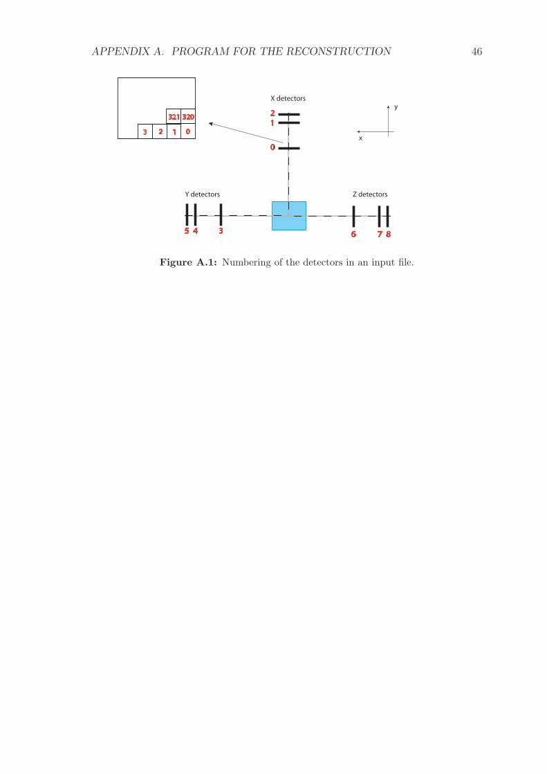
APPENDIX A. PROGRAM FOR THE RECONSTRUCTION 46

y

x

Y detectors Z detectors

X detectors

1 2

3 4 5 6 7

0

8

1 2 3 0

320 321

Figure A.1: Numbering of the detectors in an input file.

Bibliography

Agazaryan, N. et al. (2003), ‘Status report on experiment AD-4/ACE, Biological

effectiveness of antiproton annihilation’, CERN-SPSC-2003-031 .

Agostinelli, S. et al. (2003), ‘Geant4 - a simulation toolkit’, Nuclear Instruments

and Methods A 506, 250–303.

Amado, R., Cannata, F., Dedonder, J., Locher, M. and Shao, B. (1994), ‘Coherent

pion radiation from nucleon-antinucleon annihilation’, Physical review letters

72(7), 970–972.

Amsler, C. (1998), ‘Proton-antiproton annihilation and meson spectroscopy with

the crystal barrel’, Reviews of modern physics 70(4), 1293–1339.

Amsler, C. and Myhrer, F. (1991), ‘Low energy aniproton physics’, Annual review

of nuclear and particle science 41, 219–267.

Belochitskii, P., Eriksson, T. and Maury, S. (2004), ‘The CERN antiproton deceler-

ator (ad) in 2002: status, progress and machine development results’, Nuclear

instruments and methods in physics research section b-beam interactions with

materials and atoms 214, 176–180.

Degtyarenko, P., Kossov, M. and Wellisch, H.-P. (2000), ‘Chiral invariant phase

space event generator III. Modeling of real and virtual photon interactions

with nuclei below pion production threshold’, European physical journal, A

9(3), 421–424.

Eidelman, S. et al. (2004), ‘Review of particle physics 2004’, Physics Letters B

5892, 1–1109.

Gray, L. and Kalogeropoulos, T. (1984), ‘Possible biomedical applications of an-

tiproton beams: Focused radiation transfer’, Radiation Research 97, 246–252.

47

BIBLIOGRAPHY 48

Holzscheiter, M. (2004), ‘Status report on experiment AD-4, Biological effectiveness

of antiprotons’, CERN-SPSC-2004-031 .

Holzscheiter, M. (2005), ‘Status report on future plans for experiment AD-4, Bio-

logical effectiveness of antiproton annihilation’, CERN-SPSC-2005-037 .

Holzscheiter, M. et al. (2004), ‘Biological effectiveness of antiproton annihilation’,

Nuclear instruments and methods in physics research B 221, 210–214.

Horn, D. and Silver, R. (1970), ‘Distributions of charged pions’, Physical review D

2(9), 2082–2084.

Klempt, E., Batty, C. and Richard, J.-M. (2005), ‘The antinucleon–nucleon interac-

tion at low energy: Annihilation dynamics’, Physics reports 413, 197–317.

Kossov, M. (2005), ‘Simulation of antiproton-nuclear annihilation at rest’, IEEE

transactions on nuclear science 52(6), 2832–2835.

Kraft, G. (2000), ‘Tumor therapy with heavy charged particles’, Progress in particle

and nuclear physics 45, 473–544.

Weber, U., Becher, W. and Kraft, G. (2000), ‘Depth scanning for a conformal

ion beam treatment of deep seated tumours’, Physics in medicine and biol-

ogy 45(12), 3627–3641.

Wilson, R. (1946), ‘Radiological use of fast protons’, Radiology 47, 487–491.