HABITAT CONSERVATION TRUST FUND – FINAL REPORT CHARACTERISATION OF FOUR SECONDARY CHANNELS OF THE LOWER FRASER RIVER

Erica Ellis, Michael Church Department of Geography The University of British Columbia Vancouver BC V6T 1Z2 Marvin Rosenau Fisheries Centre Lower Mall Research Station The University of British Columbia Vancouver BC V6T 1Z4 31 March, 2004

HABITAT CONSERVATION TRUST FUND – FINAL REPORT Project Name: Characterisation of four secondary channels of the lower Fraser

River HCTF Project File #: 20255 Type of Report: Final Fiscal Year: April 1, 2003 to March 31, 2004 Location: Gravel reach of lower Fraser River, extending from Hope to Sumas

Mountain (60 km). Cover page photo: view of the lower Fraser River looking west (downstream), Hamilton secondary channel in foreground (L. Rempel, Sept. 20, 2002)

Executive Summary Secondary channel networks were once common features on the floodplain of large,

gravel-bed rivers (e.g. Columbia River, Colorado River, Rhine River). From an ecological perspective, they are the interface between the river and its floodplain and serve an important function in nutrient exchange, primary production and riparian habitat development. They also are widely used by fish for spawning and rearing, and provide refuge for fish and other animals during floods. From a geomorphic perspective, a well-developed secondary channel network serves to attenuate flood flows in the main channel.

Early photographic and cartographic records of lower Fraser River show an extensive system of secondary channels and active floodplain habitat. However, dykes and bank revetments, constructed since 1903 to reduce flood risk to development in this part of the floodplain, have resulted in a marked reduction in channel and floodplain width. Over the same period, populations of white sturgeon and some salmonid species known to use lower Fraser River for rearing and spawning have declined. In several regulated river systems in the United States, the loss of secondary channels and floodplain habitat has been substantial and has resulted in the near extinction of native fish populations. With a moderate amount of natural floodplain still intact, Fraser River presents an excellent opportunity for research on the geomorphology and ecology of secondary channels.

Project objectives were to characterise: (1) the hydraulic geometry, (2) the regime of flow conveyance, (3) the sedimentology, and (4) the fish community of four secondary channels in lower Fraser River. Additionally, we wished to ascertain the historical change in secondary channel extent in a sub-section of lower Fraser River. Field work was carried out during spring and summer 1999-2002 and completed in winter 2002-2003. Hydrologic and morphologic data were collected at a range of flows in study secondary channels during the 2002 freshet, to develop at-a-station hydraulic geometry relations for multiple sub-reaches within each secondary channel (corresponding to ‘upstream’, ‘mid’ and ‘downstream’ locations within the channel). Additional secondary channels were surveyed at bankfull flow to generate characteristic scaling relations for bankfull secondary channel morphology and hydraulics. Fish sampling was conducted in study secondary channels using a variety of sampling techniques, over multiple years. This project was co-ordinated with another HCTF-funded study (HCTF Project File # 2-136) to reduce costs related to field work. Change in secondary channel bank line extent to present time was quantified in a sub-section of lower Fraser River, by compiling a time-sequence comparison of bank line extent in a geographic information system (GIS). A chronology of the construction of dykes and flow-control structures over the last century in the same sub-section of the river was also developed.

Sub-reach averaged water surface width, mean hydraulic depth and mean velocity data collected in the study secondary channels generally conformed well (R2 ≥ 0.9) to the form of classical at-a-station hydraulic geometry relations, at higher flow. Spatial and frequency distributions of near-bottom velocity and channel depth were examined. In general, secondary channel sub-reach types stratified along gradients of width, depth, velocity and sedimentology, although there were exceptions. Additional data collected at high flow were used to generate bankfull scaling relations (classical downstream hydraulic geometry) for secondary channels in the gravel reach. Again, the data conform well to a simple power law up to, and including, points from the main channel.

1

The presence of 21 species of fish in the study secondary channels, including salmonid species and threatened or endangered species, confirms that secondary channels represent valuable habitat for juvenile fish. Total densities of fish at secondary channel sites are within the range of densities found in main channel sites. Fish data were stratified by their longitudinal sampling position on the gravel bar forming the bank of the secondary channel (‘up’, ‘mid’ or ‘down’). These bar position designations are the closest equivalent to the sub-reach designations used in the physical and hydraulic characterisation of the study secondary channels. Fish data did not show a strong bar position effect in the case of many metrics, suggesting that fish may not distinguish between sub-reaches within an individual secondary channel, although the sub-reaches themselves may show physical differences in morphology and hydraulics. However, species richness and proportion of salmonids demonstrate a bar position effect that suggests that certain species may prefer or avoid downstream sub-reaches in secondary channels, perhaps due to the lack of higher velocities present in more upstream locations. Overall, the fish data exhibited strong variability, which hampered our ability to discern trends in the data.

Bank line extent in a sub-section of Fraser River (Chilliwack to Agassiz, approximately) was tabulated at approximately 10-year intervals, starting with a ‘pre-settlement’ estimate (ca. 1900). Total bank line extent in each time period was divided into categories based on whether the bank line bounded a secondary channel or the main channel, and whether the bank line in question was part of an island or part of the floodplain. The total extent of bank line in the studied sub-section of the river has decreased greatly from our estimate of a pre-settlement condition to 1999 (a loss of 110 km, equivalent to a 44% decrease). This loss is largely a result of the construction of the Chilliwack dyke in 1903, which caused a loss of an estimated 108 km of bank line. Since 1903, changes in total bank line length have been minor in comparison (< 25 km change in any time period examined). After 1903, the largest changes in any time period examined have occurred in island bank line impacted by secondary channel flows (‘secondary channel/island bank line’): alternating increases and decreases of between 2 km and 20 km. These fluctuations appear to be correlated with changes in the flow regime, with periods of above-average flows leading to decreases in secondary channel/island bank line, and vice versa. The net change in secondary channel/island bank line since 1912 is a slight gain of approximately 5 km (+7%). Floodplain bank line impacted by secondary channel flows has experienced a net loss through the 20th century (19 km loss between pre-settlement and 1999, equal to a 40% decrease), with the greatest part of the decrease resulting from the construction of the 1903 dyke. Subsequent loss of secondary channel/floodplain bank line has occurred episodically as smaller islands have been incorporated into the floodplain. Changes in bank length since the completion of the Chilliwack dyke in 1903 do not suggest consistent increasing or decreasing trends over time. In fact, the total bank line extent in the studied sub-section of the river has remained relatively stable since 1912, with a net loss of 2.4 km (-1.7%).

This project is intended to complement HCTF Project # 2-136, which characterised the

physical and ecological attributes of fish habitat potentially impacted by gravel mining. Resources were shared between projects with the intent of creating an integrated body of knowledge on the ecology of the gravel reach.

2

Table of Contents

EXECUTIVE SUMMARY .........................................................................................................................................1

TABLE OF CONTENTS............................................................................................................................................3

LIST OF FIGURES.....................................................................................................................................................5

LIST OF TABLES.......................................................................................................................................................9

ACKNOWLEDGEMENTS ......................................................................................................................................10

1 INTRODUCTION............................................................................................................................................11 1.1 PROJECT RATIONALE .................................................................................................................................11 1.2 WHAT IS HYDRAULIC GEOMETRY? ............................................................................................................12

1.2.1 At-a-station hydraulic geometry ..........................................................................................................13 1.2.2 Downstream hydraulic geometry.........................................................................................................14

1.3 PROJECT OBJECTIVES................................................................................................................................17 2 METHODS AND ANALYSIS ........................................................................................................................18

2.1 STUDY SITE...............................................................................................................................................18 2.1.1 Channel and sub-reach selection.........................................................................................................20

2.2 DATA COLLECTION....................................................................................................................................21 2.2.1 Physical characterisation ....................................................................................................................21 2.2.2 Ecological characterisation.................................................................................................................25 2.2.3 Historical characterisation..................................................................................................................30

2.3 DATA ANALYSIS .......................................................................................................................................30 2.3.1 Characteristics of ADP data................................................................................................................30 2.3.2 Hydrological data analysis..................................................................................................................31 2.3.3 Sedimentological data analysis ...........................................................................................................38 2.3.4 Juvenile fish data analysis ...................................................................................................................39 2.3.5 Analysis of historical secondary channel network...............................................................................42

3 RESULTS .........................................................................................................................................................44 3.1 CHARACTERISATION OF SUB-REACH MORPHOLOGY ..................................................................................44

3.1.1 Hydraulic geometry relations ..............................................................................................................44 3.1.2 Distributions of depth and velocity......................................................................................................53 3.1.3 Sedimentological data .........................................................................................................................66

3.2 SCALING BEHAVIOUR OF SECONDARY CHANNELS .....................................................................................68 3.2.1 Relation of main-channel discharge to sub-reach discharge ..............................................................68 3.2.2 Secondary channel scaling relations ...................................................................................................71

3.3 JUVENILE FISH ..........................................................................................................................................77 3.3.1 Species abundance...............................................................................................................................78 3.3.2 Species distribution..............................................................................................................................82 3.3.3 Individual species comparisons ...........................................................................................................88

3.4 HISTORICAL SECONDARY CHANNEL NETWORK .........................................................................................90 4 DISCUSSION ...................................................................................................................................................95

4.1 SECONDARY CHANNEL MORPHOLOGY, HYDRAULICS AND ECOLOGY.........................................................95 4.1.1 Patterns in sub-reach morphology ......................................................................................................95 4.1.2 Patterns in juvenile fish data ...............................................................................................................96 4.1.3 Scaling behaviour of secondary channels............................................................................................96

4.2 TRENDS IN SECONDARY CHANNEL EXTENT ...............................................................................................99 5 CONCLUSIONS ............................................................................................................................................101

REFERENCES ........................................................................................................................................................103

3

APPENDIX A: PROJECT FINANCIAL REPORT............................................................................................107

APPENDIX B: TECHNICAL NOTES AND CALCULATIONS ......................................................................110

APPENDIX C: CONSTRUCTION OF DYKES AND FLOW-CONTROL STRUCTURES..........................122

APPENDIX D: PLOTS OF SUB-REACH AT-A-STATION HYDRAULIC GEOMETRY RELATIONS...125

APPENDIX E: PLOTS OF GRAIN-SIZE DISTRIBUTIONS...........................................................................163

APPENDIX F: RELATION OF MAIN CHANNEL TO SUB-REACH DISCHARGE...................................170

APPENDIX G: PLOTS OF FUNCTIONAL SCALING RELATIONS FOR SECONDARY CHANNELS..180

4

List of Figures Figure 1 Location map of the Lower Fraser River, BC, showing distances from Sand Heads

(km). ............................................................................................................................. 19

Figure 2 Location of secondary channels and sub-reaches where physical data were collected, either for at-a-station hydraulic geometry relations or scaling relations. Flow is from right to left. Fish data were collected in all channels used for at-a-station hydraulic geometry analysis......................................................................................................... 22

Figure 3 2002 hydrograph for the Fraser River at Hope, with approximate duration of project field work indicated (Water Survey of Canada station 08MF005). ............................. 23

Figure 4 Schematic of three channel types and eight alluvial habitat types found associated with gravel bars of lower Fraser River (after Church et al., 2000). ..................................... 26

Figure 5 Plan view of in-channel data collected on July 9th, 2002, in Jesperson channel, d/s. Note the approximate grid pattern of the ADP profiles. .............................................. 32

Figure 6 Diagram of a representative channel cross-section to illustrate the parameters involved in the calculation of discharge. A plan-view schematic (Figure 7) is required to illustrate the reduction of width data............................................................................ 34

Figure 7 Schematic detailing the reduction of ADP width data. Contrast with the cross-sectional schematic in Figure 6. Refer also to equations (17) and (18). .................... 36

Figure 8 Example of Voronoi regions used to calculate the volume of water in a given sub-reach (9-July-02, Carey m/r/d). Depths corresponding to each region are shown as small points, bank markers are shown as solid ‘x’s. .................................................... 38

Figure 9 Number (n) of fish sampling event by beach seine, gill net and minnow trap, stratified by season and longitudinal position on bar. Data were collected in secondary channels between Sept. 1999 and Sept. 2001. ‘All channels’ category includes data from the non-study secondary channels. The dashed line separates representatively fish-sampled habitats (left) from non-representatively fish-sampled habitats (right). The dotted line indicates the mean over all habitats in the ‘all channels’ category. ........... 41

Figure 10 Slopes of sub-reach hydraulic geometry width-to discharge and depth-to-discharge relations (power fit only). Note the change in scale between axes. Where separate analyses of high-flow data were performed, the slope presented is that corresponding to the high-flow data only. Non-significant slopes were not plotted and data from CAL m/r were excluded because of their irregularity.................................................. 52

Figure 11 Bivariate frequency distributions of near-bottom d/s velocity (m/s) and depth (m) for all sub-reaches in Jesperson channel at high flow (JES u/s: QMC = 10,015 m3/s, QSR = 394 m3/s; JES m/r: QMC = 10,225 m3/s, QSR = 384 m3/s; JES d/s: QMC = 10,521 m3/s, QSR = 447 m3/s). Histogram output has been converted to percent and mapped as contours of equal percent. Contour interval is variable but contours are labeled, see text for explanation. ..................................................................................................... 54

Figure 12 Bivariate frequency distributions of near-bottom d/s velocity (m/s) and depth (m) for all sub-reaches in Carey channel at high flow (CAR u/s: QMC = 9841 m3/s, QSR = 853 m3/s; CAR m/r/u: QMC = 9841 m3/s, QSR = 452 m3/s; CAR m/r/d: QMC = 9556 m3/s, QSR = 129 m3/s). Histogram output has been converted to percent and mapped as

5

contours of equal percent. Contour interval is variable but contours are labeled, see text for explanation. ..................................................................................................... 55

Figure 13 Bivariate frequency distributions of near-bottom d/s velocity (m/s) and depth (m) for all sub-reaches in Calamity channel at high flow (CAL u/s: QMC = 10,681 m3/s, QSR = 316 m3/s; CAL m/r: QMC = 10,681 m3/s, QSR = 274 m3/s; CAL d/s: QMC = 8295 m3/s, QSR = 205 m3/s). Histogram output has been converted to percent and mapped as contours of equal percent. Contour interval is variable but contours are labeled, see text for explanation. ..................................................................................................... 56

Figure 14 Bivariate frequency distributions of near-bottom d/s velocity (m/s) and depth (m) for both sub-reaches in Hamilton channel, at high flow (HAM m/r: QMC = 10,017 m3/s, QSR = 574 m3/s; HAM d/s: QMC = 10,017 m3/s, QSR = 667 m3/s). Histogram output has been converted to percent and mapped as contours of equal percent. Contour interval is variable but contours are labeled, see text for explanation. ........................ 57

Figure 15 Bivariate frequency distributions of near-bottom d/s velocity (m/s) and depth (m) for selected channels and sub-reaches, at moderate flow (JES m/r: QMC = 4615 m3/s, QSR = 94 m3/s; JES d/s: QMC = 4938 m3/s, QSR = 147 m3/s; CAR u/s: QMC = 3741 m3/s, QSR = 96 m3/s). Histogram output has been converted to percent and mapped as contours of equal percent. Contour interval is variable but contours are labeled, see text for explanation. ..................................................................................................... 58

Figure 16 Spatial distribution of (a) depth (m), (b) near-bottom d/s velocity (m/s), and (c) data points for JES u/s at high flow (QMC = 10,015 m3/s, QSR = 394 m3/s). Approximate d/s direction is indicated on (c).......................................................................................... 60

Figure 17 Spatial distribution of (a) depth (m), (b) near-bottom d/s velocity (m/s), and (c) data points for JES d/s at high flow (QMC = 10,521 m3/s, QSR = 447 m3/s). Approximate d/s direction is indicated on (c).......................................................................................... 61

Figure 18 Spatial distribution of (a) depth (m), (b) data points, and (c) near-bottom d/s velocity (m/s) for CAR m/r/u at high flow (QMC = 9841 m3/s, QSR = 452 m3/s). Approximate d/s direction is indicated on (b).................................................................................... 62

Figure 19 Spatial distribution of (a) depth (m), (b) data points, and (c) near-bottom d/s velocity (m/s) for CAR m/r/d at high flow (QMC = 9556 m3/s, QSR = 129 m3/s). Approximate d/s direction is indicated on (b).................................................................................... 63

Figure 20 Spatial distribution of (a) depth (m), (b) near-bottom d/s velocity (m/s), and (c) data points for JES d/s at moderate flow (QMC = 4938 m3/s, QSR = 147 m3/s). The additional points in (c) indicate the position of the waterline during data collection. The approximate d/s direction is indicated as well. ..................................................... 64

Figure 21 Spatial distribution of (a) depth (m), (b) data points, and (c) near-bottom d/s velocity (m/s), for CAR u/s at moderate flow (QMC = 3741 m3/s, QSR = 96 m3/s). The filled circles in (b) indicate the position of the waterline during data collection and the dashed line indicates the axis limit of (a) and (c). Approximate d/s direction is indicated as well........................................................................................................... 65

Figure 22 Comparison of different statistical models fit to JES QMC and QSR data (all sub-reaches). Main-channel ‘bankfull’ flow at which QSR will be evaluated is indicated. 70

Figure 23 Functional scaling relations for bankfull width and discharge, stratified by channel and sub-reach morphology. Bankfull at-a-station parameters are based on the high-

6

flow analyses, where performed (JES, HAM, CAR). The JES u/s data point is obscured by the JES d/s data point............................................................................... 75

Figure 24 Functional scaling relations for bankfull depth and discharge, stratified by channel and sub-reach morphology. Bankfull at-a-station parameters are based on the high-flow analyses, where performed (JES, HAM, CAR). .................................................. 76

Figure 25 Functional scaling relations for bankfull velocity and discharge, stratified by channel and sub-reach morphology. Relation was derived by continuity from the w-Q and d-Q scaling relations. Bankfull at-a-station parameters are based on the high-flow analyses, where performed (JES, HAM, CAR). CAL d/s parentheses indicate that the data quality is questionable because of a non-significant (α = 0.05) d-Q relation. ..... 77

Figure 26 Total density (mean + SE, # / m2) in beach seine samples, stratified by season, channel and position on bar. Note the change in y-axis scale between summer and winter plots. The dotted line corresponds to the average over all sites, including OTH. Number of samples (n) is indicated. ............................................................................ 79

Figure 27 Total CPUE (mean + SE, # / hr) in gill-net samples, stratified by season, channel and position on bar. Note the change in y-axis scale between summer and winter plots. The dotted line corresponds to the average over all sites, including OTH. Number of samples (n) is indicated................................................................................................ 80

Figure 28 Total CPUE (mean + SE, # / hr) in minnow trap samples, stratified by season, channel and position on bar. Note the change in y-axis scale between summer and winter plots. The dotted line corresponds to the average over all sites, including OTH. Number of samples (n) is indicated. ............................................................................ 81

Figure 29 Species richness (mean + SE), from beach seine, gill-net and minnow trap samples stratified by season, channel and position on bar. The dotted line corresponds to the average over all sites, including OTH. Number of samples (n) is indicated. ............. 83

Figure 30 Proportion of salmonid individuals (mean + SE) captured by beach seine and stratified by season, channel and position on bar. Note the change in y-axis scale between summer and winter plots. The dotted line corresponds to the average over all sites, including OTH. Number of samples (n) is indicated. ........................................ 84

Figure 31 Simpson’s diversity (mean + SE), based on beach seine data stratified by season, channel and position on bar. The dotted line corresponds to the average over all sites, including OTH. Number of samples (n) is indicated. ................................................. 85

Figure 32 Simpson’s diversity (mean + SE), based on gill-net data stratified by season, channel and position on bar. The dotted line corresponds to the average over all sites, including OTH. Number of samples (n) is provided for each average. ...................... 86

Figure 33 Simpson’s diversity (mean + SE) based on minnow trap data stratified by season, channel and position on bar. The dotted line corresponds to the average over all sites, including OTH. Number of samples (n) is indicated. ................................................. 87

Figure 34 Comparison of density (mean + SE, # / m2) and biomass (mean +SE, g / m2) for four fish species: chinook (CHI), red side shiner (RSS), peamouth chub (PEA) and large scale sucker (LGS). Data are derived from summer beach seines only. The dotted lines correspond to site averages (including OTH), and the number of samples (n) is indicated. ...................................................................................................................... 89

7

Figure 35 Assumed representation of the pre-settlement state of the study reach, based on 1912 bank lines. Study reach boundaries are indicated and the bank line classification scheme is shown........................................................................................................... 91

Figure 36 Study reach bank line classification in 1999. Location of dykes is also shown........ 92

Figure 37 Variation in bank line lengths in the study reach, over a 100-year time span. The “pre-settlement” value has been assigned an arbitrary date of 1900. .......................... 94

8

List of Tables Table 1 Level III of the habitat classification (after Church et al., 2000). Habitat abbreviations

are given in parentheses. Habitat types in italics are hypothetical only because they have not been sampled. An * denotes alluvial habitat types effectively sampled by beach seine. .................................................................................................................. 28

Table 2 Fish species known to occupy the gravel reach of Fraser River for some portion of the year and 3-letter codes assigned to those species captured in this study between 1999 and 2001. ...................................................................................................................... 29

Table 3 'Downstream' direction (referenced to true North) for all sub-reaches. ......................... 35

Table 4 Sub-reach hydraulic geometry relations for Jesperson channel. .................................... 46

Table 5 Sub-reach hydraulic geometry relations for Carey channel. .......................................... 47

Table 6 Sub-reach hydraulic geometry relations for Hamilton channel. .................................... 48

Table 7 Sub-reach hydraulic geometry relations for Calamity channel...................................... 49

Table 8 Surface grain-size parameters, all sub-reaches. ............................................................. 68

Table 9 Sub-surface grain-size parameters. ................................................................................ 68

Table 10 Relation of sub-reach discharges to main-channel discharge (at Hope). ..................... 71

Table 11 Computed sub-reach bankfull (BF) estimates of discharge (m3/s), water surface width (m), mean depth (m), mean velocity (m/s), and associated uncertainty a. ......... 72

Table 12 Functional scaling relations for secondary channel bankfull parameters. ................... 73

Table 13 Study reach bank line lengths (km) in various categories, from approximately 1900 to 1999.............................................................................................................................. 90

Table 14 Changes in bank line category lengths (km) between study years, including totals over all study years, and a total since 1912.......................................................................... 93

Table 15 Comparison of selected downstream hydraulic geometry relations (scaling relations)....................................................................................................................................... 97

9

Acknowledgements Funding for this project was provided by The Habitat Conservation Trust Fund. E. Ellis

received personal support from the National Sciences and Engineering Research Council. The former British Columbia Ministry of Fisheries (now Ministry of Water, Land and Air Protection, WLAP) provided a jet boat and accommodation during periods of field work, at the Fraser Valley Trout Hatchery in Abbotsford. Field sampling equipment was provided by the Department of Geography, University of British Columbia, and the former BC Ministry of Environment, Lands and Parks (WLAP). The following people are gratefully acknowledged for field assistance: Dave Awram, Chris Ayles, Sara Barker, Dave Campbell, Cathy Christie, Mike Church, Brett Eaton, Margaret Ellis, Fly, Darren Ham, Alexis Heaton, Kris Holm, Andrew Luke, Shawn Johnston, Bob Land, Bob Lee, Nick Manklow, Jacqui Morrisson, Dave Oldmeadow, Mike Papageorge, Teri Peterson, Jason Rempel, Dr. Steve Rice, Karyn Rilkoff, Catherine Shaw, Ian Skipper, Blair Tarling, Hamish Weatherly, Arelia Werner, Andre Zimmerman and Zip. Tara Flundra (City of Chilliwack), Kelly Harms (Chilliwack Archives), and Neil Peters (WLAP) provided important information regarding historical dyking activity on the lower Fraser River. Laura Rempel (UBC Geography) and Darren Ham (UBC Geography) provided data and invaluable technical assistance in producing this report.

10

1 Introduction

1.1 Project rationale World-wide fragmentation and regulation of natural river systems is leading to loss of

river ecosystems and riverine species (Dynesius and Nilsson, 1994). Riverine floodplains, including secondary channel networks, are some of the most productive and biologically diverse ecosystems on earth (Tockner and Stanford, 2002). Natural ecosystem processes in floodplains facilitate clean water and provide renewable timber, fisheries, and wildlife resources. In addition, they naturally attenuate high flows. However, historically floodplains have also been a locus for human settlement, agriculture and industry. Processes of natural channel change are now increasingly viewed as a threat to the high densities of people and capital investment along river corridors. For this reason, large rivers in particular have been the attention of much engineering work to straighten, maintain and dyke channel courses. This activity has resulted in a dramatic simplification of historically complex and productive habitat, a trend that will likely continue into the future (Tockner and Stanford, 2002).

Evidence suggests that secondary channel networks of large rivers are an endangered

habitat whose ecological function is important but poorly characterised (Bayley, 1995; Jungwirth et al., 2002; Tockner and Stanford, 2002). The gravel-reach of lower Fraser River presents an excellent opportunity for research on the geomorphology and ecology of secondary channels. In this reach, the river flows over a partially confined, cobble-gravel fan (Church and McLean, 1994). The channel assumes a laterally unstable, wandering morphology as a consequence of gravel transport through the reach. This morphology is generally characterised by an irregularly sinuous main channel that flows around island-bar complexes and creates secondary channels (Desloges and Church, 1989). In Fraser River, secondary channels (i.e., channels other than the main channel) form a network within the floodplain of the river, consisting of:

1. ‘side channels’ - mostly relatively short and large secondary channels, which flow around vegetated islands and gravel bars in the active main channel zone. These channels have a flow regime that varies from highly seasonal in smaller channels, to perennial in larger channels.

2. ‘anabranches’- relatively long, narrow and stable channels (including sloughs), flowing around large vegetated islands

The term ‘anabranch’ refers to narrow channels associated with large, stable islands, which persist for decades or centuries and support well-established vegetation (Knighton, 1998). Few ‘anabranch’ channels currently remain in a freely flowing state in the lower Fraser River, although this channel type was common in the early part of the 20th century. Most have been cut-off from the main channel at their upstream entrances as a result of dyking, or are affected by flow-control structures (e.g., weirs).

The arrangement of secondary channels is dynamic through time, changing as the river modifies its channel through the transport and deposition of sediment. Based on observations of river dynamics documented by air photos, secondary channels in lower Fraser River typically develop as the flow divides around large deposits of sediment (bars). Island growth occurs on bars that develop to sufficient height to cause slack water over their tops, even at highest flows. Slack water encourages the deposition of finer sediments, thus increasing the height of the surface even more. Eventually, vegetation becomes established on the surface, which further encourages the trapping of fine sediments. Once established, islands may persist for centuries

11

before they are eventually attacked by the flow and removed. The persistence of islands is largely linked to the alignment of the main channel, since major erosion events are unlikely to occur away from the main channel. There are many examples of island growth in lower Fraser River during the period of record (i.e., ca. 1871 to present), of a variety of sizes of islands (e.g., Church and Weatherly, 1998). Secondary channel dynamics are primarily linked to island dynamics, since islands (or complexes of islands and bars) provide the boundaries for secondary channels. Where islands have remained stable for many decades, secondary channels may begin to fill in with finer sediments, and vegetation may encroach along the banks, creating a typically narrower channel than might be observed in an area where the river is more active. This is a possible mechanism for the transition of a ‘side channel’ to an ‘anabranch’.

Within the gravel reach of Fraser River, British Columbia’s largest population of pink salmon (Onchorhynchus gorbuscha) spawn in odd years and high densities of juvenile chinook salmon (O. tshawytscha) rear throughout the year. Preliminary research by L. Rempel (HCTF Project # 2-136) has shown that secondary channels provide rearing habitat for 20 fish species. HCTF-supported research has also found that white sturgeon (Acipenser transmontanus, red-listed in BC) primarily use secondary channels for spawning (Perrin et al., 2000; Perrin et al., 2003a). Vegetated banks along secondary channels provide extensive near-shore habitat for fish where cover, drop-in terrestrial insect prey, nutrients and microhabitat features are found.

Bank hardening, dyking and isolation of the floodplain have resulted in much loss of

secondary channel habitat in lower Fraser River over the last century, primarily impacting ‘anabranch’ channels. However, the ‘side channel’ network remains relatively intact, and therefore presents an exceptional opportunity for scientific research to thoroughly characterise the ecological and physical attributes of these secondary channels. There is continuing pressure on the gravel reach of lower Fraser River, which relates to flood protection. Various actions being considered are gravel mining from within the active channel, upgrading dykes, and adding riprap and revetments to resist bank erosion. These measures, when applied together and persistently, may ultimately lead to further reduction of secondary channel area and degradation of habitat quality (Church and McLean, 1994). Data collected in this study can serve not only as a baseline state for Fraser River, and also as a useful template for the increasing number of river restoration projects being undertaken globally (e.g. Simons et al., 2001; Buijse et al., 2002).

1.2 What is hydraulic geometry? Hydraulic geometry is an attempt to describe the adjustment of the cross-sectional form

of stream channels by scaling with discharge (Q). The general relations are assumed to be power functions of the independent variable, Q, as follows:

ws = aQb, where ws is water surface width (1)

d* = cQf, where d* is the mean hydraulic depth (2)

v = kQm, where v is mean velocity (3)

S = gQz, where S is channel slope (4)

(Leopold and Maddock, 1953).

12

Other channel parameters have been used as dependent variables, including flow resistance and suspended sediment load. The exponents describe the rate of change of the given channel parameter with discharge whereas the coefficients define a value of the dependent variable for unit discharge.

The width, mean depth and mean velocity are related by continuity:

Q = w × d × v, (5)

which implies:

b + f + m ≡ 1.0, and (6)

a × c × k ≡ 1.0 (7)

Thus there are only two independent relations amongst ws, d* and v that together determine the third relation.

The concept of hydraulic geometry was first developed and applied to rivers in the mid 20th century in a seminal paper by Leopold and Maddock (1953). Data from a variety of gauging stations in the Great Plains and Southwest of the United States were used to show that water surface width, mean depth and mean velocity plotted as simple power functions (and hence, scaling functions) of discharge. This outcome was interpreted as indicating an equilibrium relation between the channel form and the flow conveyed.

Leopold and Maddock envisioned channel adjustment occurring in two different ways: 1) a channel cross-section or reach might be adjusted to accommodate the range of flows

experienced at that location (termed “at-a-station” or “at-a-point” hydraulic geometry); 2) the river channel might be adjusted along its length to increasing flows resulting from

increasing downstream drainage area (termed “downstream” hydraulic geometry). Although at-a-station hydraulic geometry and downstream hydraulic geometry share a similar method of graphical representation, the consensus of present research is that they are essentially different (Ferguson, 1986; Clifford, 1996), both in terms of underlying mechanics and application.

1.2.1 At-a-station hydraulic geometry As discharge increases or decreases at a given point along a river, there are characteristic

corresponding changes in water surface elevation (stage), velocity, width and depth. This knowledge has long been applied in the use of stage-discharge relations, or rating curves, to facilitate measurement of discharge. Extending this idea, Leopold and Maddock found approximately log-linear relations between mean width, depth and velocity and discharge for their 20 study reaches (which represent a variety of rivers) and gave average values for the exponents: b = 0.26, f = 0.40 and m = 0.34 (1953). It has been customary to use gauging section data to develop at-a-station hydraulic geometry relations because these data are readily available.

The implication of the power law relation between channel parameters and discharge is that the observed channel form is in equilibrium with the forcing function, discharge. However, it is clear that, in the case of an individual cross-section or reach, the form of the channel is

13

dictated in large part by the most recent competent flow. Lesser flows simply occupy the predetermined space without substantially altering it. Therefore, an equilibrium relation is unlikely to exist in any meaningful sense between channel parameters and the entire range of flows experienced at that cross-section, given that the majority of those flows will not exceed the competence threshold. The derived relations are not true power laws, although they are tolerably well described by simple power laws. Given the natural variability in channel cross-section properties as a result of factors such as meandering, pool-riffle sequences and changes in bank resistance, it is not surprising that there should be large variability in at-a-station hydraulic geometry exponents and coefficients, with no obvious pattern (Park, 1977).

However, the variability induced by site-specific characteristics means that the at-a-station relations reflect individual channel characteristics. The capability of hydraulic geometry relations to offer a concise, quantitative description of channel form has many useful applications, mainly in river management (Mosley, 1982; Hogan and Church, 1989; Jowett, 1998). At-a-station relations quickly summarise the adjustment in mean channel characteristics with changing discharge. This permits the comparison of different channels or the assessment of particular channels based on physical habitat requirements (e.g. “depth-velocity” curves, for fish species). For instance, whether channels accommodate increasing discharge primarily in increasing depth or width will greatly affect the type of habitat that exists at different discharges. However, the use of mean values of channel parameters, and gathering of data at single cross-sections (which has been the norm) means that important information about the variability within the habitat is lost by averaging. For instance, the use of mean velocity in aquatic habitat modeling is much less appropriate than the so-called “nose velocity”, which expresses the velocities commonly experienced by fish (Stalnaker et al., 1989).

Consequently, part of the information necessary for useful habitat assessment is the distribution of velocity-depth products over a range of flows. When combined with water surface area, these data give a “disaggregated hydraulic geometry” (Hogan and Church, 1989) which can be used to make a graphic comparison of the areal or frequency distribution of velocities and depths over changing flows, and between streams. With knowledge of particular species’ life cycle habitat preferences, disaggregated hydraulic geometry can be used to evaluate the potential of different streams, or different reaches within streams, to provide appropriate habitat. Alternatively, combining disaggregated hydraulic geometry relations for particular reaches with knowledge of the resident species allows conclusions to be made about habitat preference and use.

1.2.2 Downstream hydraulic geometry Equilibrium channel form in designed channels Although the concept of hydraulic geometry in natural channels was novel, Leopold and Maddock were explicitly influenced by research in the late 19th century on the designed channel form of stable canals. The purpose of this research was to develop a set of equations that could be used to design unlined irrigation canals, given a certain imposed discharge, slope and sediment load, which would neither silt up nor scour their beds. These stable channels were termed to be “in regime” with their governing conditions, from which derives the name “regime theory” for this body of work. Regime theory deals with equilibrium channel form in canals flowing through fine sands and silts, which were designed to carry a certain sediment and water load. Therefore, it is equivalent to the “downstream” case in hydraulic geometry. The related tractive force method deals with the form

14

of designed, stable channels in coarse materials for the limiting case of no sediment transport. For a stable channel to exist in non-cohesive coarse material, the channel form must be such that the distribution of shear force never exceeds the critical shear force to induce motion. It is possible to calculate the theoretical narrowest stable channel cross-section such that everywhere sediment is on the verge of motion (the so-called threshold channel), in which the stability of the banks imposes the lower limit on stability. Lane and Carlson (1953) analysed a series of stable canals in coarse-grained material and offered design guidelines including a factor to account for bank stability, based on side slope and natural angle of repose of the sediment.

Simons and Albertson (1963) attempted to extend the range of conditions over which the regime-type equations would apply by collecting data on canals in India (primarily fine-grained materials) and ones in the United States (coarser-grained materials). These channels would be classified as dominantly sand-bed channels, as 22 of 24 reaches analysed had a median bed-material grain diameter of less than 1 mm. The reaches were stratified based on bed and bank composition, and then channel parameters were graphically displayed as functions of discharge. The interesting result is that variability in the derived relations between channel parameters and discharge was dominantly expressed in the coefficients of the relations. For channels with a sand bed and cohesive banks, the relation between wetted-perimeter and discharge is (in ft-sec units):

P = 2.51Q0.512 (8)

Less cohesive channels plotted above this relation and more cohesive channels plotted below it. Therefore, the coefficients of the relations appear to play an important role in reflecting variation in bed and bank composition.

A substantial body of literature exists on the subject of designed equilibrium channels, from which some trends emerge such as the consistent one-half power relation of channel width to discharge. Also, results from designed channels suggest that variation in bed and bank composition induces variability in the coefficients of the hydraulic geometry relations. However, these designed channels are a simplified representation of natural channels, and as such have fewer degrees of freedom to adjust their form. In natural channels, discharge varies, reaches are not always straight, channel pattern varies, within-channel morphology changes and bank vegetation is present, all adding extra variability to adjustments of channel form. Equilibrium form in natural channels As formulated by Leopold and Maddock (1953), downstream hydraulic geometry relations express the adjustment of a river channel in space to increasing flow due to tributary and groundwater inputs. However, there are relatively few examples of empirical downstream hydraulic geometry relations on individual main-stem channels, due to the difficulty of gathering sufficient data on any one river. Instead, data have typically been gathered from a number of different rivers from similar physiographic settings. By stratifying natural channels by physiography, it is assumed that similar boundary conditions exist within the group. It is assumed that physiographical stratification yields “regime classes” within which rivers will exhibit similar channel-forming behaviour.

Data must then be gathered from the different channels at some reference discharge that occurs with the same frequency at all stations. Although theoretically a variety of flow frequencies could be examined (cf., Leopold and Maddock, 1953), the convention is to define the reference flow to be the most regularly occurring flow which has the potential to change the cross-sectional form of the channel (through erosion and sediment transport). Leopold and

15

Maddock, using the mean annual flow as the reference discharge, found an average downstream hydraulic geometry for their study reaches yielding exponents of b = 0.5, f = 0.4 and m = 0.1. In terms of the relation of width to discharge, this study confirmed the one-half power trend observed in the regime canals.

In effect, downstream hydraulic geometry relations can be thought of as scaling relations for channel form: ws is a suitable choice for a scale length and the cross-sectional area of flow, A, defines a storage-discharge relation:

A = rQt (9)

The other relations of hydraulic geometry follow by continuity, since

A/ws = d* (10)

and

Q/A = v (11)

One might reasonably expect that there could be an equilibrium relation between natural

channel form and some measure of a recurring, channel-shaping flow. This is borne out in the occurrence of large-scale trends such as the characteristic relations of width and depth to discharge (Figure 9 in Leopold and Maddock (1953); Figure 8 in Ferguson (1986)). Nonetheless, as with the at-a-station relations, there remains notable scatter in the downstream hydraulic relations (Park, 1977; Ferguson, 1986). Some of the scatter may be due to different reference flows used to derive the relations. More substantively, the cross-sectional form of a natural channel will depend on the particular balance struck between the erosive forces of the flow and the resistive forces of the channel boundaries. Therefore, as in regime theory, we may expect that similar hydraulic geometry relations will exist for channels with similar sedimentological characteristics, all else being equal, with the variation between groups being expressed in the coefficients of the relations.

Bank vegetation obviously has an important role to play as far as increasing resistance to erosion. Vegetation increases bank strength through the binding effects of its root mass, reduces near-bank velocities and effective shear stress, and encourages the deposition of fine material during overbank flows. In general, it has been found that vegetated banks result in narrower and deeper channels than ones with less stable banks (Millar and Quick, 1993; Huang and Nanson, 1997; Millar, 2000).

One additional difference between natural channels and designed channels is the ability of natural channels to adjust to changes in boundary conditions by changing their channel pattern. In an attempt to reduce potential variability induced by this consideration, most empirical research has focused on single-thread, straight channels, or, at most, straight single-channel reaches within a multi-channel river (Bray, 1973; Griffiths, 1981; Andrews, 1984). In addition, some work has been done on braided channels. Braided rivers are defined here as having multiple channels separated by bars that are commonly submerged at high flows and bounded by floodplain banks. Little work has been accomplished on the anabranches of multi-thread channels.

16

1.3 Project Objectives Project objectives are as follows:

a) Conduct spatially-distributed cross-sectional surveys of at-a-station hydraulic geometry (water surface width, water depth, water velocity) in four secondary channels to quantify the hydraulic characteristics of fish habitat, the flow conveyance capacity, and frequency of inundation.

b) Utilise at-a-station hydraulic data to construct spatial maps and bivariate frequency distributions of near-bottom velocity and depth, to characterise fish habitat.

c) Conduct similar surveys of channel geometry in additional channels at bankfull flow in order to develop characteristic scaling relations for bankfull secondary channel form in lower Fraser River (i.e., classical downstream hydraulic geometry relations).

d) Conduct surface and sub-surface sampling of sediments in secondary channels to characterise substrates encountered by fish.

e) Sample fish in four secondary channels to quantify relative use and to determine species composition of fish in these channels.

f) Ascertain the historical extent of secondary channels in a sub-section of lower Fraser River. Quantify changes in secondary channel habitat extent and connectivity over the 20th century.

17

2 Methods and Analysis

2.1 Study Site The study site is located in the gravel reach of the Lower Fraser River, in southwestern

British Columbia. The Fraser River drains about 25% of British Columbia (228,000 km², measured at Mission) and the mainstem is unregulated along its length. The hydrograph is dominated by the snowmelt freshet, which normally occurs in early June, though timing varies depending on the meteorological conditions influencing snowmelt. The river ranks highly on a global scale as a producer of salmonine fishes (Northcote and Larkin, 1989).

The Lower Fraser River extends from Yale to the Pacific Ocean (~ 190 km) (Figure 1),

and exhibits three distinct morphologies along this length. Between Yale and Laidlaw, the river channel is single-thread, and confined. The substrate is coarse gravel and cobble. Once it emerges from the confines of the mountains, the river flows over a partially-confined cobble-gravel fan. This gives rise to a characteristic wandering channel morphology between Laidlaw and Sumas Mountain (termed the “gravel reach”). Within this reach of the river there is a clearly defined main channel as well as secondary channels, which flow around and across large island-bar complexes. At Sumas Mtn., the river morphology changes back to a single-thread channel, and switches abruptly to a sand-bed.

The at-a-station hydraulic geometry of the unconstrained main channel is known at two

locations: Agassiz and Mission. These locations correspond to reaches where the channel is single-thread, and where the bed composition is, respectively, gravel and sand. Gauging stations also provide a lengthy record of discharge at these two locations. The mean annual flood at Agassiz is 8,760 m3/s and at Mission is 9,790 m3/s (McLean et al., 1999). The hydraulic geometry at Hope is also known, although the channel is rock-confined at this location.

A distinctive feature of wandering rivers is their seasonally persistent secondary

channels. In these relatively smaller channels comparatively lower flows result in the whole channel being potentially suitable habitat for different species. In contrast, within large channels (e.g. main channels) lateral zonation creates areas of hydraulic efficiency (the thalweg of the channel) and areas of biological richness (the shore zone), the relative location and size of which are conditioned by the magnitude of the discharge (Stalnaker et al., 1989). The presence of these laterally-shifting habitat zones has been verified with reference to invertebrate habitat in the main channel of the Fraser River before, during and after the yearly freshet (Rempel et al., 1999). It is theorized that the persistent secondary channels in the Fraser River provide refuge habitat for fish during high flows and may also provide valuable rearing habitat for juvenile fish. Ongoing research by Rempel is demonstrating the exceptionally diverse ecosystem represented in part by secondary channels of the Fraser River. Recent research indicates that these channels are also used as spawning habitat by endangered white sturgeon (Acipenser transmontanus) (Perrin et al., 2000; Perrin et al., 2003a).

18

Figure 1 Location map of the Lower Fraser River, BC, showing distances from Sand Heads (km).

19

Visual examination of secondary channels in the Fraser River suggests that there may be characteristic sub-reaches within each channel, each exhibiting distinctive hydraulic and sedimentological characteristics. Flow divergence into secondary channels at the upstream entrance produces a shallow and fast sub-reach with primarily gravel and cobble bed material. Conversely, at the downstream confluence of a secondary channel and the main channel, there is a backwater effect, which produces an “estuarine”, deep and slow-flowing sub-reach with primarily fine bed sediment. A third sub-reach incorporates the transition from upstream to downstream and is intermediate in character between the upstream and downstream reach types. In larger secondary channels this is the most extended sub-reach, and may express the most characteristic geometry of such channels, given the space to develop.

2.1.1 Channel and sub-reach selection Secondary channels were chosen for physical characterisation based on the logistics of

access and hydraulic sampling, as well as prior fish sampling effort in the channels. The channels had to be located relatively near to one another in order to keep main-channel travel time to a minimum. In addition, channels had to be free from obstructions that would prevent access to sub-reaches in low-flow conditions. Fish sampling in lower Fraser River began in the summer of 1999 (HCTF Project #2-136), and therefore potential channels were also evaluated on the basis of fish data availability. Four secondary channels were chosen within the gravel reach for physical and ecological characterisation: Calamity (CAL), Carey (CAR), Hamilton (HAM) and Jesperson (JES). Of the four study channels, Calamity channel flows behind the smallest and most recently formed gravel bar. It is constrained on the right bank by bedrock outcrops at the u/s and d/s ends of the channel. It is also downstream of the confluence of Fraser River and Harrison River (the only major tributary in the gravel reach). Jesperson channel (also known as Greyell Slough) is the oldest and longest of the study channels, and flows behind a large island-bar complex. Flow is controlled at the upstream end of the channel by a weir established approximately thirty years ago. Carey channel and Hamilton channel are intermediate in age and length between Calamity and Jesperson. Hamilton channel is controlled along the right bank by rip-rap. It is the site of the former main channel from approximately 1930 to 1950 (see Figure 6 in McLean and Church, 1999). A railroad runs along the upstream half of Carey channel and the right bank is protected by old rip-rap along the length of the tracks. Of the four channels, Jesperson had not been used for fish sampling in 1999 or 2000. However the documented presence of endangered white sturgeon spawning in this channel (Perrin et al., 2000; Perrin et al., 2003a) suggests that it has significant ecological value, and that a detailed physical characterisation would be valuable.

Of all the study channels analysed in this report, Jesperson channel most strongly

resembles the ‘anabranch’ secondary channel type, whereas Calamity, Carey and Hamilton are good examples of the ‘side channel’ secondary channel type defined in Section 1.1. However, in the interest of brevity, for the remainder of this report the study channels will be referred to generally as ‘secondary channels’.

Rather than collecting hydraulic data at a single cross-section, sampling areas were

established within each secondary channel to represent the upstream (u/s), mid (m/r) and downstream (d/s) sub-reach morphology, based on visual assessment in the field. Sub-reach length varied between 75 m and 200 m depending on the scale of the channel. The four channels used for at-a-station hydraulic geometry data collection yielded 13 sub-reaches (Carey channel

20

was sufficiently long to have two “mid” sub-reaches of different character). Five additional channels were chosen to study the scaling relations: Grassy, Queens, Minto, Big Bar and Gill. One sampling area was established in each of these channels to represent the mid-channel sub-reach morphology. The channels sampled solely for the scaling relation data range in size, but are generally larger secondary channels than the study secondary channels (Grassy is comparable in size to the study channels). A deliberate effort was made to choose larger secondary channels in which to collect data for the scaling relations, in order to incorporate as wide a range of discharges as possible. Figure 2 shows the location of all channels and sub-reaches where data collection occurred. A careful examination of Figure 2 will show that the sub-reaches in Carey channel and Hamilton channel are separated by additional minor channels flowing diagonally across the bar surface, connecting the behind-bar study channel to the main channel. Therefore, there are additions (Hamilton) or losses (Carey) of discharge between sub-reaches when these across-bar channels are active.

2.2 Data collection

2.2.1 Physical characterisation A wide range of discharges is desirable to develop at-a-station hydraulic geometry

relations, because of the power-form of the relation. For the purposes of the scaling relations, data collection at a scaling flow close to bankfull is most appropriate. Although the actual magnitude of the freshet is not fully predictable, both of the previous concerns suggested that data collection for this project should begin slightly before the estimated peak of the hydrograph, and should continue on the declining limb of the flood. The declining limb of the hydrograph is often less-steeply inclined than the rising limb, allowing more time for data collection, although this was not the case in 2002. Sub-reaches were established preceding the 2002 freshet and reference surveys of permanent and semi-permanent markers were conducted between March and May 2002. These markers were used to measure water surface width, water surface slope, and stage.

The 2002 freshet had a peak daily average discharge of 10,681 m3/s at Hope, on June 21 (Figure 3), that corresponds approximately to the 5-year flood. After the snowmelt peak, there were very few inputs of precipitation and therefore the flow declined steadily and rapidly through July and August. Hydraulic data collection in the secondary channels began in May 2002 and continued through the summer and autumn, as long as the channels were flowing. All sedimentological data were collected in the winter following the freshet, between February and March 2003, when secondary channels were predominantly dry. In addition, all reference surveys of sub-reach markers were repeated during the winter period to include the high-water markers added during the freshet. At-a-station hydraulic geometry relations Starting in late May 2002, at-a-station sub-reaches were surveyed on a continuous rotation through the freshet. Of a total 13 sub-reaches, two (from two different channels) had to be discarded during data collection because of logistics. One sub-reach simply ceased to exist when the bar, which defined the left bank, was eroded away (Carey Channel, d/s), and the other became impossible to navigate because of the volume of gravel moved into the middle of the channel (Hamilton Channel, u/s).

21

Figure 2 Location of secondary channels and sub-reaches where physical data were collected, either for at-a-station hydraulic geometry

relations or scaling relations. Flow is from right to left. Fish data were collected in all channels used for at-a-station hydraulic geometry analysis.

22

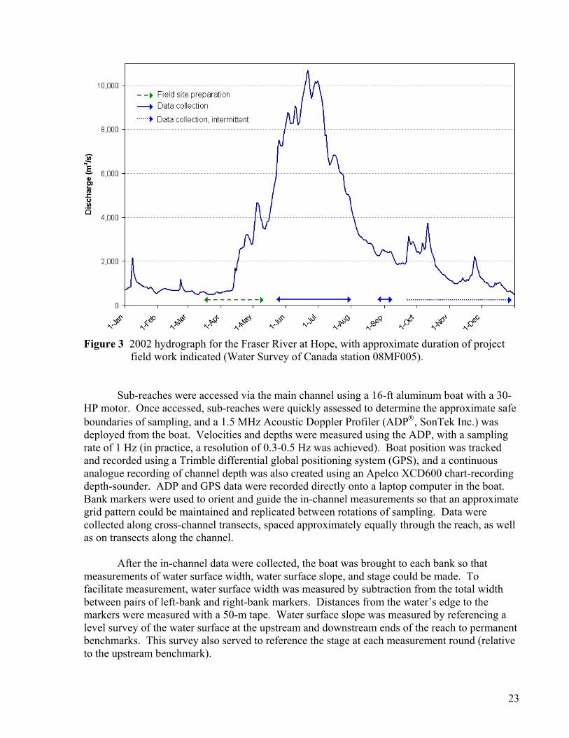
Figure 3 2002 hydrograph for the Fraser River at Hope, with approximate duration of project

field work indicated (Water Survey of Canada station 08MF005).

Sub-reaches were accessed via the main channel using a 16-ft aluminum boat with a 30-HP motor. Once accessed, sub-reaches were quickly assessed to determine the approximate safe boundaries of sampling, and a 1.5 MHz Acoustic Doppler Profiler (ADP, SonTek Inc.) was deployed from the boat. Velocities and depths were measured using the ADP, with a sampling rate of 1 Hz (in practice, a resolution of 0.3-0.5 Hz was achieved). Boat position was tracked and recorded using a Trimble differential global positioning system (GPS), and a continuous analogue recording of channel depth was also created using an Apelco XCD600 chart-recording depth-sounder. ADP and GPS data were recorded directly onto a laptop computer in the boat. Bank markers were used to orient and guide the in-channel measurements so that an approximate grid pattern could be maintained and replicated between rotations of sampling. Data were collected along cross-channel transects, spaced approximately equally through the reach, as well as on transects along the channel.

After the in-channel data were collected, the boat was brought to each bank so that

measurements of water surface width, water surface slope, and stage could be made. To facilitate measurement, water surface width was measured by subtraction from the total width between pairs of left-bank and right-bank markers. Distances from the water’s edge to the markers were measured with a 50-m tape. Water surface slope was measured by referencing a level survey of the water surface at the upstream and downstream ends of the reach to permanent benchmarks. This survey also served to reference the stage at each measurement round (relative to the upstream benchmark).

23

Bank markers originally were placed along the bankfull channel edge (defined as the beginning of permanent, woody vegetation). However, in most reaches the flow was above bankfull at and around the peak of the freshet, and submerged many bank markers. New markers were established to reference width, slope and stage measurements, where possible. Original markers were relocated after the freshet receded, although in some cases the markers were irretrievable. A second reference survey was conducted following the freshet to tie all remaining markers together. Although an attempt was always made during overbank flows to measure the true extent of the water surface (including standing water in the overbank vegetation), the presence of thick vegetation and bank levees often made this impossible. In most cases, flow through the vegetation was minimal compared with in-channel flow.

In some sub-reaches, near-shore access became impossible with the ADP as the freshet

declined. Near-shore velocity and depth measurements were then collected with a hand-held electromagnetic velocity meter (Flo-Mate Model 2000, Marsh-McBirney Inc.) and top-set wading rod. These measurements were taken at each width marker, and paced at approximately 1 or 2-m intervals into the channel from the waterline, up to the depth at which wading became impractical (and boating was possible): slightly over 1 m. Mean velocity and total depth were recorded at each measurement position. Secondary channel scaling relations Additional data collection for the channel scaling relations occurred in five different channels, covering a range of channel sizes (Figure 2). Sub-reaches were established to represent the intermediate “mid” reach morphology. In-channel ADP data were collected once only, while flow was near bankfull. The primary concern was to be able to collect data as quickly as possible, so that the flow would not have changed substantially during the time required to sample all the channels. For that purpose, it was decided that a water surface width measurement could be obtained at a later date either through photogrammetry (since the bankfull flow extended to the edge of vegetation on both banks) or from the GPS data collected at the time. A subsequent round of visits to these reaches was used to establish markers at the upstream and downstream ends of the reaches that were used for the water surface slope survey. A level survey was conducted at a later date to tie the markers together. Surface and sub-surface sedimentology Sedimentological data were collected at low flow in winter following the 2002 freshet. In each of the at-a-station and scaling relation sub-reaches, 400-stone grid counts were conducted to derive an estimate of surface roughness (Church et al., 1987). Material was sized in half-phi increments down to 8 mm, and the number of counts of sand was also recorded. If the bed was wholly composed of sand or finer sediment, a sample was taken for sieve analysis.

In addition, a bulk sample was taken in the upstream sub-reach of each at-a-station

channel to characterise the sub-surface sedimentology, following the sample size protocol suggested in Church et al. (1987). Material was hand-sized or sieved and weighed in the field down to 16 mm or 22 mm and the remaining sediment was randomly split until a sub-sample of the appropriate weight was achieved (based on the 0.1% criterion in Church et al., 1987). This sample was returned to the lab for processing. Effort was made to sample sediment that had been moved into reaches during the preceding freshet, so as to estimate the size distribution of sediment in transport. New sediment transported into the channel after the 2002 freshet was

24

distinguished based on visual assessment since the sediment tends to be deposited in coherent sheets, with prominent slip faces at their downstream edges. The sediment on which the new sheets rested was then categorised as being the ‘old’ channel surface.

2.2.2 Ecological characterisation The distribution and abundance of juvenile fish in secondary channels were examined

using various capture techniques, including netting by beach seine (12.5 m × 2 m, 6 mm knotless mesh), gill netting (three-panel net with mesh sizes of 2.5, 4, and 7 cm), and minnow trapping. Sampling for fish in secondary channels was carried out in summer (April – September) and winter (October – March), between 1999 and 2001. This work was supported by HCTF as Project File #2-136.

Fish sampling targeted specific habitat types, as delineated in Level Three of the Morphological and Habitat Classification of the Lower Fraser River Gravel-Bed Reach (Church et al., 2000). These habitat types are represented in Figure 4 and defined in Table 1. Habitats are recognised as being physically and ecologically distinct from each other, and occur throughout the gravel reach. They are distinguished based on morphology and are visually recognisable in the field. Different habitats lend themselves to different sampling methods, although the majority of habitat types were effectively sampled by beach seine. Certain habitats presented logistical problems that precluded the use of the beach seine (e.g. very deep water, cut-banks, etc.), and in these habitats either gill nets or minnow traps were used.

A 17-foot aluminium-welded boat with an outboard jet engine, on loan from the former BC Ministry of Fisheries, was used to travel on the river between sites. Sampling by beach seine occurred within habitat units by dragging the net in a downstream direction along the shoreline. Samples were collected over a distance of 10 – 50 m, depending on the length of the habitat unit. Fish became trapped in the net, which was then hauled on shore. The contents were promptly examined and all fish were immediately transferred to holding buckets containing fresh river water.

Gill netting was restricted to habitats of deep, standing water away from the main channel to minimise the risk of intercepting migratory salmon. The small mesh sizes also reduced this risk. As a consequence, the habitats sampled by gill net were distinct from those sampled by beach seine and gill net catch data were used mostly as supplementary information on the distribution of species in the gravel reach. Nets were set at the water surface and were clearly marked with floats and permit identification while left fishing in the river. Daytime sets averaged 2 hr in duration whereas night time sets averaged 18 hr (winter months only). Fish were then removed from the net as carefully as possible to minimise injury, and immediately transferred to holding buckets containing fresh river water for recovery and processing.

25

Figure 4 Schematic of three channel types and eight alluvial habitat types found associated with gravel bars of lower Fraser River (after Church et al., 2000).

Minnow traps were used extensively during winter months when beach seine sampling was less effective. Traps often were set where both beach seines and gillnetting were not feasible such as surrounding large woody debris accumulations and along densely vegetated island banks. Because the traps were baited with salmon roe, they did not provide representative catch information (some species are “trap-shy” and some species are more attracted to the bait). Nevertheless, the data were of interest as supplementary information on the distribution of species in the gravel reach. Traps were clearly marked with floats and anchored with lead weight to the bottom while fishing. Daytime sets averaged 5 hr, however most traps were left overnight and set duration averaged 19 hr. Fish were removed from the trap and immediately transferred to holding buckets containing fresh river water for processing.

Once collected, all fish were identified to species according to McPhail and Carveth

(1994) and counted. A minimum of 15 fishes representing each species in the haul were measured for fork length (mm) and weighed (g). Over 7,000 fish were caught and identified in the four study channels in this study. From this data set, twenty-one species of fish were identified (Table 2), including eight salmonid species and three blue-listed species (mountain sucker, coastal cutthroat trout, and brassy minnow). Although white sturgeon are known to use secondary channels for spawning (Perrin et al., 2000; Perrin et al., 2003a), we did not catch or observe any while sampling.

26

All fish sampling methods have associated catch biases. Gill netting is biased based on the net mesh size, which determines the size range of fish captured. Minnow traps are biased both towards a size range of captured fish, determined by the trap opening, and the species collected. Beach seining may be considered to be the least biased of the three methods, although mesh size determines the lower size limit of fish caught and some species may be particularly skilled at evading the net. In general, turbidity during most months of seining is believed to have minimised sampling bias. To reduce fish evasion of the net, each seine was executed swiftly and only relatively short lengths of beach were sampled at a time. The catch data were discarded for any seine in which the net became snagged. Despite these efforts, it remains probable that bottom-dwelling fish managed to evade the net in some instances, particularly over coarse substrate. Highly agile and fast-swimming fish may have evaded the net in some instances as well. The problem of fish escaping through the net pertains only to very small individuals (< 20 mm) whose species identification would be difficult, and to small individuals of longnose dace that are highly streamlined and could pass through the mesh. Clear water in winter months (October – March) likely contributed to an underestimate of fish density.

27

Table 1 Level III of the habitat classification (after Church et al., 2000). Habitat abbreviations are given in parentheses. Habitat types in italics are hypothetical only because they have not been sampled. An * denotes alluvial habitat types effectively sampled by beach seine.

HABITAT TYPE DEFINITION

Riffle (RI) High-gradient area of shallow, fast water flowing over well-sorted substrate that often has granular structures and is stable. The flow is rough. Common at bar heads.

Bar Head (BH)* Upstream end of a gravel bar. Surface substrate is characteristically coarse and flow velocity is usually high (erosional) but can be a back eddy (depositional).

Bar Edge (BE)* Any length of bar edge not occurring at the head or tail of a bar that is oriented parallel to the flow and subject to constant and consistent flow forces. Bank slope is variable and a range of velocities and substrate types is possible. Riparian influence is variable.

Bar Tail (BT)* Downstream end of a gravel bar, usually with moderate flow velocity. The habitat is often depositional and surface substrate consists of smaller cobbles and gravels.

Eddy Pool (EP)* Area bounded by fast, rough water that creates a back eddy in the lee of the flow. Common on the inside edge of riffles and at the upstream end of some bar head habitats. Bank slope is invariably steep and the substrate is usually embedded cobble.

Open Nook (ON)* Shallow indentation along a bar edge of reduced velocity and variable substrate that is openly connected to the channel with no sedimentary barrier (unlike channel nook). An ephemeral habitat that often disappears with a relatively small change in water level.

Channel Nook (CN)* Dead-end channel or narrow embayment of standing water and concave geometry. Substrate material usually consists of sand/silt and embedded gravel.

Bay (BA)* Semi-enclosed area with no flow velocity and fine bed material (sand/silt). Occurs on the lee side of large sediment accretions that are deposited in the shape of a crescent-dune.

Bar Top (BT)+ Bar top surface inundated only during high flow with reduced velocity and shallow water depth relative to open water and the thalweg. Substrate is variable.

Vegetation (VG) + Area of flooded island and bank vegetation where velocity is reduced and substrate is relatively fine. Submerged only at very high flow.

Cut Bank (CB) Eroding bank of fine sediment that is steeply sloped or vertical. Dense riparian vegetation is often present. Large woody debris is common and flow conditions are variable.

Rock Bank (RB) Natural rock bank, possibly with openings and cracks, that is invariably steep. The water is deep immediately offshore and currents are either fast or form a back eddy.

Artificial Bank (RP) Bank is invariably steep and consists of riprap or rubble rock that may have significant openings within its structure. The water is usually deep and fast immediately offshore.

Open Water (OP) Open area with no direct influence from bank or bar edge features or riparian vegetation. Velocity and substrate characteristics are variable.

* alluvial habitat types effectively sampled in this study. + hypothetical habitat – not sampled

28

Table 2 Fish species known to occupy the gravel reach of Fraser River for some portion of the year and 3-letter codes assigned to those species captured in this study between 1999 and 2001.

Family Species Common name Code Acipenseridae Acipenser transmontanus White sturgeon R nc Salmonidae Prosopium williamsoni Mountain whitefish MWF Salvelinus confluentus Bull trout B nc S. malma Dolly Varden B nc Onchorynchus clarki Cutthroat trout B CUT O. gairdneri Rainbow trout RBT O. gorbuscha Pink salmon PIN O. keta Chum salmon CHU O. kisutch Coho salmon COH O. nerka Sockeye salmon SOC O. tshawytscha Chinook salmon CHI Cyprinidae Hybognathus hankinsoni Brassy minnowB BRA Mylocheilus caurinus Peamouth PEA Ptychocheilus oregonensis Northern pikeminnow NPM Rhinichthys cataractae Longnose dace LND R. falcatus Leopard dace LED Richardsonius balteatus Redside shiner RSS Catostomidae Catostomus macrocheilus Largescale sucker LGS C. platyrhynchus Mountain sucker B MTS C. columbianus Bridgelip sucker nc Gasterosteidae Gasterosteus aculeatus Threespine stickleback TSS G. aculeatus trachurus Marine stickleback MSB Cottidae Cottus aleuticus Coastrange sculpin CRS C. asper Prickly sculpin PRS Petromyzonidae Lampetra ayresi River lamprey+ LAM L. richardsoni Western brook lamprey+ LAM L. tridentata Pacific lamprey+ LAM Osmeridae Thaleichthys pacificus EulachonB * nc

R: red-listed, B: blue-listed + specimens captured in this study were not identified to species, presence documented in Northcote and Larkin

(1989) * presence upstream of Agassiz documented by Perrin et al. (2003b) nc: not captured in this study

29

2.2.3 Historical characterisation A portion of the Fraser River gravel reach, which encompasses the four study channels,

was chosen for a GIS-based analysis. The boundaries of the study area correspond approximately with the boundaries of Figure 2: the upstream boundary is the Agassiz-Rosedale Bridge (slightly upstream of the boundary of the figure) and the downstream boundary is Chilliwack Mountain (in the lower left corner of the figure).

Air photos covering the study reach were selected at approximately ten-year intervals, to 1999. The earliest air photos were taken in 1928. The historical time period was extended by including a planimetric map based on a 1912 survey, which is the earliest accurately-scaled record of channel and island locations. Air photos were digitised using an analytical stereoplotter. For each time period, the location of river features such as bank lines (main channel and secondary channels), gravel bars, and islands were mapped. This information was then imported into a geographic information system (GIS) for analysis.

To assess changes in connectivity between secondary channels and the main channel, the location of all flow control structures, such as dykes and weirs was also digitised, where discernible. A chronology of the construction of these structures was developed by consultation with provincial and local officials, as well as archival records.

2.3 Data Analysis Data processing, analysis and graphical display of hydraulic data were performed using

MATLAB version 6.5.1. Historical bank line analysis was performed using Arc/Info 8.3.

2.3.1 Characteristics of ADP data The ADP is a monostatic current meter (i.e., the same transducer functions as a

transmitter and a receiver), which operates using the principle of the Doppler effect. Rather than measure the water velocity per se, the ADP measures the Doppler shift of sound reflected from particles in the water column. Particles in the water column are assumed to be moving with the flow, and therefore one must assume that their motion is equivalent to the water motion. The ADP used in this study has three beams each oriented at 25° off the vertical axis and at 120° relative azimuth to each other. By measuring the Doppler shift in each beam, the three-dimensional water velocity can be calculated using geometry. Although these velocity data are originally calculated with respect to a Cartesian co-ordinate system relative to the ADP, they can be converted to a geographically referenced system (East-North-Up, or ENU) by using data from the internal compass. Data are collected in user-specified depth bins that start after a blanking region immediately in front of the transducers. All together, data describe a complete vertical profile of velocity.

With every ADP profile, the following data were collected: date, time water velocities in each of the ENU components, for each depth bin signal strength by beam, for each depth bin water temperature compass and tilt sensor data

30

bottom-track data (where possible) GPS data (where possible)

More detail on ADP measurements can be found in Appendix B. Boat-velocity reference When collecting data from a moving platform, the water velocity that the ADP measures is a combination of the motion of the water (or particles in the water) and the motion of the platform. Therefore, to know the water velocity we need a method to derive the platform velocity. There are currently two options available: (1) GPS data or (2) the ADP bottom-tracking (BT) function.

To use GPS data as a boat-velocity reference, the GPS is normally integrated into the ADP data-collection apparatus and a position fix is taken at the beginning and end of each profile. The boat velocity is then calculated as the change in position over the time interval. When the bottom-tracking option is used, the ADP uses a separate pulse to locate the channel bottom. The Doppler shift from this pulse is used to infer the motion of the platform relative to the channel bottom. GPS and bottom-tracking can be enabled simultaneously during data collection, allowing two independent boat-velocity estimates to be compared.

The accuracy of boat-velocity estimates referenced to the GPS is determined by the differential accuracy of the GPS unit. The differential signal for the unit we used was received by antenna from a beacon located approximately 120 km distant. This may have been close to the limit for reliable signal reception, as we had problems consistently receiving the beacon signal. Topography and proximity to heavily vegetated banks also may have influenced our signal reception. When signal reception was poor, the GPS was incapable of resolving the relatively small motion of the boat between profiles and was therefore not an acceptable boat-velocity reference.

According to the manufacturer of the ADP, it is preferable to reference boat-velocity to the bottom-tracking algorithm, as they consider it to be more accurate (B.Macone, pers.comm. 2003, T.Mudge, pers.comm. 2004). However, given that bottom-tracking returns the motion of the platform relative to the bottom, if the bottom is mobile than the boat-velocity estimate will be biased (i.e. sediment moving downstream will cause an apparent boat motion in the upstream direction). Significant sediment transport would typically not occur in smaller channels with coarse beds, except at very high flows. However, in channels with sandy beds, bottom-tracking bias may become a factor. In those cases, the boat-velocity should be referenced to the GPS if possible.

2.3.2 Hydrological data analysis Estimates of discharge through each sub-reach were required to derive hydraulic

geometry relations. These discharge estimates were based on the ADP data collected in the field. The first method devised to calculate discharge through the at-a-station sub-reaches relies on reasonably good bottom-tracking coverage and at least partial GPS signal reception. Other methods were derived to deal with measurements in which data of this quality were not available.

31

Due to the deliberate spatial distribution of in-channel measurements, it was possible to derive multiple estimates of discharge for each round of measurements in a sub-reach. For example, in the case of the measurements in Figure 5, a discharge estimate was generated for each cross-channel line and then the distribution of estimates within the reach was examined.

Calculation of discharge through a cross-channel line followed a specific methodology. Consider the channel cross-section in Figure 6. Each vertical line in the schematic represents a velocity and depth profile as measured by the ADP. These profiles are separated by non-standard width increments, the size of which is dictated by boat-speed and data quality. The total discharge through the cross-section (QXS) is equal to the sum of the discharges through the middle and edges of the channel:

QXS = QLB + QADP + QRB (12)

The mid-channel (i.e. QADP) and bank components of the total discharge were calculated using different methods according to what boat velocity reference information was available, as summarised below and detailed in Appendix B.

Figure 5 Plan view of in-channel data collected on July 9th, 2002, in Jesperson channel, d/s.

Note the approximate grid pattern of the ADP profiles. Method 1: Files with good bottom-tracking and good GPS signal reception.

The output from Method 1 yields two separate discharge estimates. The calculation is identical for each estimate but in one only BT-referenced velocities are used, and in the other

32

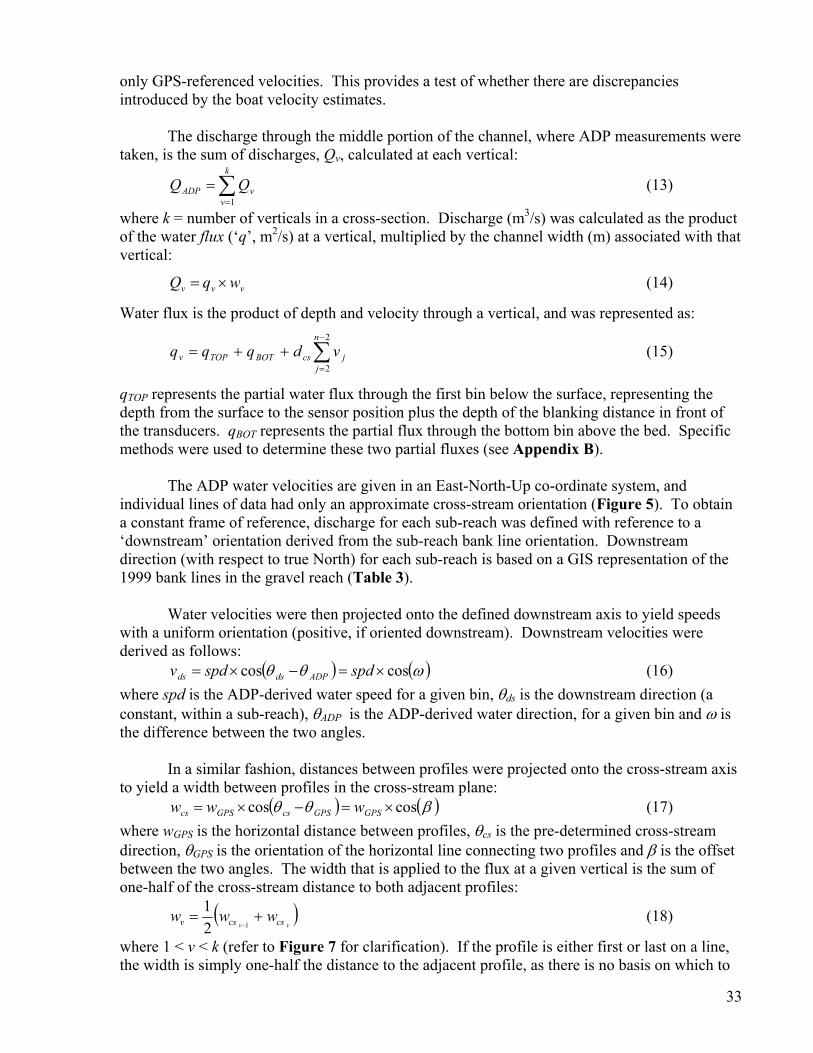
only GPS-referenced velocities. This provides a test of whether there are discrepancies introduced by the boat velocity estimates.

The discharge through the middle portion of the channel, where ADP measurements were taken, is the sum of discharges, Qv, calculated at each vertical:

∑=

=k

vvADP QQ

1 (13)

where k = number of verticals in a cross-section. Discharge (m3/s) was calculated as the product of the water flux (‘q’, m2/s) at a vertical, multiplied by the channel width (m) associated with that vertical:

vvv wqQ ×= (14)

Water flux is the product of depth and velocity through a vertical, and was represented as:

∑−

=

++=2

2

n

jjcsBOTTOPv vdqqq (15)

qTOP represents the partial water flux through the first bin below the surface, representing the depth from the surface to the sensor position plus the depth of the blanking distance in front of the transducers. qBOT represents the partial flux through the bottom bin above the bed. Specific methods were used to determine these two partial fluxes (see Appendix B).

The ADP water velocities are given in an East-North-Up co-ordinate system, and individual lines of data had only an approximate cross-stream orientation (Figure 5). To obtain a constant frame of reference, discharge for each sub-reach was defined with reference to a ‘downstream’ orientation derived from the sub-reach bank line orientation. Downstream direction (with respect to true North) for each sub-reach is based on a GIS representation of the 1999 bank lines in the gravel reach (Table 3).

Water velocities were then projected onto the defined downstream axis to yield speeds with a uniform orientation (positive, if oriented downstream). Downstream velocities were derived as follows:

( ) ( )ωθθ coscos ×=−×= spdspdv ADPdsds (16) where spd is the ADP-derived water speed for a given bin, θds is the downstream direction (a constant, within a sub-reach), θADP is the ADP-derived water direction, for a given bin and ω is the difference between the two angles.

In a similar fashion, distances between profiles were projected onto the cross-stream axis to yield a width between profiles in the cross-stream plane:

( ) ( )βθθ coscos ×=−×= GPSGPScsGPScs www (17) where wGPS is the horizontal distance between profiles, θcs is the pre-determined cross-stream direction, θGPS is the orientation of the horizontal line connecting two profiles and β is the offset between the two angles. The width that is applied to the flux at a given vertical is the sum of one-half of the cross-stream distance to both adjacent profiles:

(vv cscsv www +=

−121 ) (18)

where 1 < v < k (refer to Figure 7 for clarification). If the profile is either first or last on a line, the width is simply one-half the distance to the adjacent profile, as there is no basis on which to

33

assign a representative shoreward width. Discharge through the channel edges is handled in a separate calculation.

Figure 6 Diagram of a representative channel cross-section to illustrate the parameters involved

in the calculation of discharge. A plan-view schematic (Figure 7) is required to illustrate the reduction of width data.

The discharge calculation for the near-shore areas of the channel is slightly different than that used in the middle part of the channel.

(a) Extrapolation to zero When channel geometry and flow conditions permitted boating into near-shore locations

with the ADP, the bank discharge was estimated by a simple extrapolation of the last (or first) ADP flux to zero at the waterline.

(b) Near-shore velocity measurements Where it was considered that a substantial portion of the near-shore channel was not

adequately represented by the ADP measurements, hand-held velocity meter measurements were taken (see Section 2.2.1).

34

Table 3 'Downstream' direction (referenced to true North) for all sub-reaches.

channel & sub-reach downstream (°) a

Calamity – u/s 260.0 Calamity – mid 269.5 Calamity – d/s 217.6

Carey – u/s 269.5 Carey – u/s mid 269.5 Carey – d/s mid 246.1 Jesperson – u/s 241.3 Jesperson – mid 272.0 Jesperson – d/s 338.3 Hamilton – mid 311.7 Hamilton – d/s 273.7 Queens – mid 225.2 Grassy – mid 227.9 Minto – mid 211.2 Gill – mid 277.4 Big – mid 282.7

a based on GIS map of 1999 bank lines Method 2: Files with sparse bottom-tracking and good GPS signal reception.

Where bottom-tracking coverage was poor but the GPS signal was of good quality, all profiles with good GPS are included, whether or not they have bottom-tracking. When using ADP data with no bottom-tracking signal, it is necessary to have an alternate measure of channel depth. Data from the chart-recording depth sounder were used for this purpose. Details of this method can be found in Appendix B. Method 3: Files with good bottom-tracking and no GPS signal reception.

There were a number of rounds of measurements in different sub-reaches that lacked reliable GPS position data. In addition, many of these reaches had sparse bottom-tracking coverage. In some cases, poor GPS reception affected every round of measurements made in a particular sub-reach (e.g. Hamilton d/s). In order to salvage these measurements, depths were taken from the depth-sounder, water velocities were referenced to bottom-tracking (when available) and water surface widths were derived from on-shore measurements.

35

Figure 7 Schematic detailing the reduction of ADP width data. Contrast with the cross-

sectional schematic in Figure 6. Refer also to equations (17) and (18).

The digitized depth-sounder charts were integrated and then divided by the length of the chart to obtain an average depth for the navigable part of the channel (dCHART). A mounting depth of 0.155 m was added to the average. An average was taken for all cross-sectional lines to obtain the average dCHART for the sub-reach. Velocities were treated in a fashion identical to Method 1 (and Method 2) and projected into the imposed downstream plane. Profiles were truncated based on bottom-tracking (where available) and then profile averages were created for those profiles with bottom-tracking coverage. Finally, an average downstream velocity over all valid profiles was calculated. Water surface widths measured during the on-shore survey were used to calculate an average width for the sub-reach. Widths were truncated in a manner similar to that applied in Methods 1 and 2 for overbank flows. Discharge was calculated simply as the product of the average depth, width and velocity and cross-sectional area was calculated as the product of the average width and depth.

In order to test how well the results of Method 3 might agree with Method 1, Method 3 was applied to two sub-reaches with good bottom-tracking and GPS signal reception (Jesperson d/s and Carey u/s). The comparison is given in Appendix B.

36

Method 4: Low-flow measurements.

In many of the sub-reaches, boating became impossible before the channel had stopped flowing completely. Either the sub-reach was not accessible by boat or it was impractical to deploy the ADP in the sub-reach because of shallow water depths. In these cases, an attempt was made to collect the necessary velocity data to calculate discharge by using the hand-held velocity meter. Data were collected in a manner similar to near-shore velocity measurements and simply carried on to the opposite bank, if possible. Due to variations in channel depth within individual sub-reaches, it was not always possible to collect velocity data at more than one cross-section, although this was always attempted. Correction for compass bias The ADP has an internal compass that enables velocities, which are originally referenced to the ADP’s internal geometry, to be converted to a geomagnetic frame of reference. Inaccuracies in the compass will result in an inaccurate direction being assigned to velocity measurements, hence may create biased estimates of downstream and cross-stream velocity components. Although the compass was properly calibrated before each ADP deployment, an examination of the velocity data after the discharge analysis was complete revealed the presence of a persistent compass bias. Where possible, this bias was accounted for by applying a correction to the d/s velocity. For the most part, the mean corrections were quite small: ± 0 – 3%. For details on the determination of and correction for compass bias, see Appendix B. Derivation of “reach-averaged” channel parameters The intent of this project was to collect data in a distributed fashion over an area of channel, rather than relying on a single cross-section. Spatial averaging could then be performed by estimating the volume of water sampled within the sub-reach, and dividing by the sub-reach length to determine a reach-averaged cross-sectional area of flow. A regular pattern of cross-sectional and longitudinal data-collection lines was maintained to facilitate the calculation of discharge. However, the density of longitudinal lines was much less than that of the cross-sectional lines, due to time constraints during data-collection.

Given the irregular spacing between depth and velocity measurements, averaging over the reach had to incorporate a weighting scheme to emphasize those data in lightly-sampled areas of the channel. We decided to use Voronoi regions (also called Thiessen polygons) to calculate what portion of the total sub-reach area was closest to each point, and to use that area as a weight. Points representing zero depth (i.e. the waterline) were included at the end of each cross-sectional line. A boundary representing the left-bank and right-bank waterline and upstream-most and downstream-most markers was then imposed on the Voronoi regions to truncate them. The volume of water in the sub-reach was then calculated as the sum of the products of all truncated Voronoi region areas multiplied by their corresponding depth measurement. The average cross-sectional area was determined by dividing the volume by the average of the left-bank and right-bank sub-reach lengths (to account for any bank curvature).

There were difficulties in implementing this methodology to calculate volume. In particular, the density of data points in the sub-reach often overwhelmed the MATLAB “Voronoi” algorithm. The problem appeared to be two-fold: the large number of points in general was problematic, and also the tendency for the points to be closely spaced or even co-

37

located, either along lines or because lines overlapped accidentally. In order to allow the algorithm to run successfully, first the cross-sectional data were thinned by excluding every other point (usually this was a sufficient thinning but in a few cases only every third point could be included). Once a stable configuration had been achieved, the longitudinal points and waterline points were added and Voronoi regions were calculated again. If the algorithm failed at this point, the longitudinal data were thinned on the basis of proximity to the nearest cross-sectional or waterline point until a second, stable configuration was reached. If the longitudinal data points were too closely spaced (e.g. when collecting data and attempting to make headway against the current), the data were manually thinned until the algorithm ran successfully.

Figure 8 shows one example of Voronoi regions calculated for the d/s mid sub-reach of Carey channel, at moderately high flow. The regions are relatively homogeneous in size, except near the right (North) bank where they are slightly larger. Heavy overhanging bank vegetation prevented the boat from accessing the near-shore area on this bank.

580780 580800 580820 580840 580860 580880 580900 5809205453280

5453290

5453300

5453310

5453320

5453330

5453340

5453350

5453360

5453370

Easting (m)

Nor

thin

g (m

)

Avg. XS area is 108.5 m 2 .

Figure 8 Example of Voronoi regions used to calculate the volume of water in a given sub-

reach (9-July-02, Carey m/r/d). Depths corresponding to each region are shown as small points, bank markers are shown as solid ‘x’s.

2.3.3 Sedimentological data analysis Surface sedimentology Samples were collected, sized in half-phi intervals and tabulated in the field. Grain-size distribution curves were created for each sample and size parameters such as the median grain-size (D50) were interpolated from each curve.

In the case of fine material (both bank sand samples and pipe dredge samples), the field samples were dried at 200°C for 24 hours and then sieved into half-phi categories down to

38

0.063 mm (phi = 4). Dredge samples were further sized using a sedigraph analysis. Sedigraph samples comprised material < 0.125 mm and were first burned in a muffle-furnace at 450°C for 4 hours to remove organic material (which can cause problems for the sedigraph). The sedigraph record was used to separate the material into half-phi increments down to 0.5 µm. A composite grain-size distribution was then developed for the original sample. Sub-surface sedimentology Field samples were dried at 200°C for 24 hours and then sieved into half-phi categories down to 0.063 mm (phi = 4). A composite grain-size distribution was developed based on the field weights and the laboratory weights. Size parameters were interpolated from the grain-size distribution curves.

2.3.4 Juvenile fish data analysis Due to the shared resources between HCTF Project #2-136 and this project, fish sampling

was conducted in the four study secondary channels as well as several other secondary channels in the gravel reach. For the purposes of this analysis, the data were grouped by study channel (i.e., CAL, CAR, HAM and JES). Those data collected in non-study channels were combined into a fifth category (OTH), which represents an average condition of secondary channels in the gravel reach.

Over the sampling period, a total of 267 samples were collected in the study channels by beach seine, gill net and minnow trap (515 samples, when all secondary channels are included). Sampling was more intensive in the summer. Fish sampling locations referenced the island-bar complex that forms the bank of the secondary channel in question (e.g., a fish sample taken in Calamity secondary channel would refer to Calamity bar as the sampling location). The general position of each fish sample along the longitudinal extent of the bar, from upstream to downstream, was recorded with each sample (e.g., ‘up’, ‘mid’ or ‘down’). These designations correspond approximately to the sub-reach designations used in the physical characterisation of the study channels (‘upstream’, ‘mid reach’, and ‘downstream’), although hydrologic and morphologic data were not collected concurrently with the fish data. Fish data were further stratified by season: summer (April to September) or winter (October to March).

Grouping of fish data by their longitudinal position on the bar allows comparisons to be made between fish species composition and the physical characterisation of the secondary channel sub-reaches (e.g., do secondary channel sub-reaches that are physically distinct have different species assemblages as well?). However, it is recognised that a single bar position or sub-reach designation may encompass multiple habitats (as defined in Section 2.2.2). Although analysing the data at the habitat level was not practical due to small sample sizes, habitats tend to stratify along a hydrological gradient, and this gradient is also implicit in the bar position designation. Therefore, a link can be made between habitat types and bar position. Figure 9 shows the number of samples collected in each habitat type for both seasons and all bar positions. In each plot, the dashed line separates habitats that were representatively sampled (left) from those that were not (right). The hydrologic gradient is indicated for representatively sampled habitats. Habitats that are ‘exposed’ tend to experience faster-flowing water, and therefore also have relatively larger bed sediment. Habitats that are more sheltered have correspondingly slower water velocities and therefore, finer substrates.

39

The change in sampling intensity between summer and winter is obvious in Figure 9 (note the change in y-axis scale). This is explained partially by the seasonal nature of the flow conditions in most secondary channels: the majority of secondary channels are not flowing in winter and flow generally stops during late summer or early fall. Once the secondary channels have ceased flowing, standing water may be present in the downstream ends, which accounts for the relatively high proportion of winter samples in the ‘down’ position, as compared to the ‘up’ and ‘mid’ positions.

The following parameters, or metrics, were calculated to assess differences in the fish community between the study channels and between the different positions in the channels. Formulae are from Krebs (1998). 1) Density: total number of fish captured in a beach seine haul, divided by the sampling area

(# / m2).

2) Biomass density: total weight of fish captured in a beach seine haul, divided by the sampling area (g / m2).

3) Catch per unit effort (CPUE): total number of fish captured in a gill-net or minnow-trap, divided by the duration of the set (# / hr).

4) Species Richness: total number of unique species captured in a sample (all sampling methods).

5) Salmonid Index: the proportion of all individuals belonging to the family Salmonidae (Table 2).

6) Simpson’s Diversity (D’): where p is the proportion of individuals of

the i

∑=

−=−=s

iipDD

1

211'th species. D refers to Simpson’s Index. The index provides more weighting for

common species and reflects the probability of picking two fish at random that are different species. Values range from 0 to 1.

The data were grouped by sampling method before calculating most fish community

metrics, to avoid combining biased (gill net, minnow trap) and more representative (beach seine) sampling methods. This grouping was not applied in the case of species richness, because species richness is intended to indicate the number of species known to occur in the habitat type, irrespective of their proportional representation in the total catch. Grouping sampling methods to calculate species richness provides the most complete habitat-specific estimate of the total number of species present at any one time or position along the channel. The salmonid index was calculated only for beach seine data, because salmonid species were rarely caught by the alternate methods.

40

Figure 9 Number (n) of fish sampling event by beach seine, gill net and minnow trap, stratified by season and longitudinal position on bar.

Data were collected in secondary channels between Sept. 1999 and Sept. 2001. ‘All channels’ category includes data from the non-study secondary channels. The dashed line separates representatively fish-sampled habitats (left) from non-representatively fish-sampled habitats (right). The dotted line indicates the mean over all habitats in the ‘all channels’ category.

41

Comparisons of the summer plots in Figure 9 show evidence of a bar-scale hydraulic gradient between up, mid and down bar positions. ‘Representatively’ fish sampled habitat types (see Figure 9) present during any given sampling period were sampled proportionately, and therefore the number of samples is an indication of the tendency of a habitat unit to be found at a particular position along the bar. Habitats that are designated ‘exposed’ are relatively more common in the ‘up’ bar position, whereas ‘sheltered’ habitats are found in greater numbers in the ‘down’ bar position. Although the bar edge habitat appears relatively more common in the ‘down’ position of the study channels, in fact it probably takes on the more sheltered character of other habitats there. This habitat type tends to have relatively high variability in its physical characteristics. The link between position on bar and the hydraulic gradient suggests that stratifying data by position on the bar should not introduce large variability due to lumping habitats, since the proportional representation of habitats shows stratification at the bar scale.

2.3.5 Analysis of historical secondary channel network Air photos were digitised using an analytical stereoplotter. For each time period, the

location of river features such as bank lines (main channel and secondary channels), gravel bars, and islands were mapped. After importing the digitised channel features to the GIS, channel bank lines were selected and assigned a numeric code based on their inferred immediate flow environment (i.e., main channel or secondary channel). It is hypothesised that one important function of secondary channels is to serve as rearing habitats for juvenile fish, by providing refuge from the relatively faster flows in main channel habitats. For the purposes of the GIS-based analysis, secondary channels are considered to be all channels other than the main channel, flowing behind vegetated islands, or island-gravel bar complexes, which are connected to the main channel at both ends. The flow environment adjacent to a given bank line was assessed visually in the GIS. Bank lines were then categorised to distinguish their immediate flow environment, and also to distinguish whether the bank line was part of an island, or floodplain:

(a) main channel flow, impacting floodplain bank line

(b) main channel flow, impacting island bank line

(c) secondary channel flow, impacting island bank line

(d) secondary channel flow, impacting floodplain bank line The total bank line length (km) in each category was summarised for each time period. The total thalweg length (km) within the study area was also measured in the GIS for the same time period. The path of the thalweg was visually estimated, and three separate estimates were averaged to produce the final result. Bank line lengths and thalweg lengths were used to create measures of bank line km per river km (i.e., per thalweg km), both for the total bank line length, and for each category of bank line. The total bank line length per river km has been used to indicate the connectivity and extent of a river’s secondary channel network, since it provides a measure of the length of shoreline along which the river and floodplain intersect (e.g., Sedell and Froggatt, 1984). By sub-dividing the bank lines into categories, we can identify trends in the total bank line extent at a finer resolution.

Changes in bank line extent can be linked to either channel dynamics of island creation and erosion, or human impacts such as dykes. Dyking of the secondary channel network began at the time of settlement, in the late 19th century. With the backing of the Provincial Government, a major dyking project to protect the town of Chilliwack and surrounding area, was

42

undertaken in 1899 and completed in 1903 (see Table C-1, in Appendix C). Therefore, on our earliest map (which is based on a 1912 survey), the dyke is already present and impacts the connectivity of the secondary channel network. In order to represent the secondary channel network in a pre-settlement state, we chose to simply analyse the 1912 network without considering the dykes. We refer to this as the estimated ‘pre-1903’ state of the secondary channel network. The Fraser River gauge at Hope was established in 1912, and therefore it is impossible to evaluate the peak flows between 1903 and 1912 in order to assess how much the river might have changed in that time period, and hence how representative our pre-1903 estimate is likely to be.

For the purposes of the analysis, once a secondary channel was closed off at its upstream end, it was no longer considered to be extant, and the entire length of channel was erased. Some remnants of the pre-1903 secondary channels persisted in the form of sloughs or back channels. However, it can be difficult to determine accurately their effective upstream limits from air photos, due to dense vegetation growth along their banks. The truncation of blocked secondary channels means that total bank length estimates are conservative, although the estimate is accurate if one is considering only secondary channels with upstream and downstream connectivity to the main channel.

43

3 Results

3.1 Characterisation of sub-reach morphology Using the hydraulic and sedimentological data collected in this study, it is possible to

create characterisations of sub-reach morphology that encompass flow hydraulics, channel shape and substrate texture. The most compact summary of the channel shape and hydraulics data is in the form of at-a-station hydraulic geometry relations, which will be presented in the following section. Because the data were collected over an area of channel, it is also possible to generate maps showing the spatial distribution of velocities and depths within a given sub-reach. These data can be represented as bivariate histograms of joint velocity and depth distribution. Finally, surface and (in some cases) sub-surface grain-size distribution curves can be presented for each sub-reach.

3.1.1 Hydraulic geometry relations Once all data files had been analysed using one of Methods 1-4, and the output had been

corrected for compass bias (where possible), the corrected output was used to create at-a-station hydraulic geometry relations. Given the nature of the classical at-a-station relations, we require only an estimate of discharge as well as two of the three available parameters (i.e. surface width, hydraulic mean depth and mean velocity). The third relation should then be estimated by continuity from the other two. It seems logical that we should use the two parameters which are known with the least error, or which are known most directly. In the case of this study, the water surface width was the parameter which was measured most directly and which was known with low error. The remaining two parameters were derived by less direct means. Based on the collected water depth data, a volume of water was calculated for each round of measurements in a sub-reach. The volume divided by the shore length that it represented provided an average cross-sectional area for the sub-reach. From the average cross-sectional area, the water surface width and the discharge both the hydraulic mean depth and the mean velocity were derived. However, it seemed that the depths had less associated error than the velocity measurements, and therefore the at-a-station relations for average velocity were derived from continuity from the water surface width and hydraulic mean depth relations, using equations (6) and (7).

The at-a-station relations were derived using functional analysis, rather than simple least-squares regression. The functional analysis should be used in situations such as this where we desire to estimate the parameters of a curve either for descriptive or comparative purposes (Mark and Church, 1977). Regression would have been inappropriate since the ‘predictor’ datum is not known without error. The functional analysis will fall somewhere between the conventional regression line and the inverse regression (i.e. a regression where ‘Y’ is used to predict ‘X’). The factor used to convert a regression to a functional relation is the ratio of error variances:

2

2

x

y

E

E=λ (19)

As the error in the ‘X’ variable goes to zero, λ approaches infinity and the functional relation approaches the conventional regression. If the relations are strong and R2 is high (e.g. > 0.9), the difference between the regression and the functional analysis is not great.

Estimates of error in the hydraulic geometry variables are therefore necessary for the functional analysis. A detailed error analysis was conducted for each discharge estimate and

44

calculated errors were most often smaller than the actual scatter in the data about the best fit line (represented by the standard error of the mean over all cross-section estimates). This result suggests either that the errors were underestimated or that there are additional sources of error not accounted for in the error analysis. A third possibility is the presence of real, unreduced random or systematic variance in the data. The standard error of the mean of the discharge estimate was used to represent the error in this variable. For all other variables, errors were assigned on the basis of the error analyses that were performed.

For the relation of width to discharge and the relation of depth to discharge, λ was calculated by averaging the fractional error of both parameters over all rounds and calculating the appropriate ratio of errors. These values are given in the tables of results (see Table 4 – 8).

The results of the functional analyses are presented for each sub-reach, in a tabulated form. A complete record of the figures corresponding to each relation can be found in Appendix D, which includes plots of residuals. The power form is the conventional form chosen to represent the at-a-station hydraulic geometry relations, but there is no a priori reason why it must be used (Ferguson, 1986). Each relation was developed using the power form but if there was significant lack of fit in the residuals, a linear fit was also attempted. If the linear fit improved the goodness of fit (as assessed by the R², SEE and residuals plot), it was also presented in the table of results.

In some sub-reaches (JES, CAR and HAM), data collected at lower flows showed a lack of agreement with the trend of the (relatively) higher flow data, indicating the potential effect of residual width and depth when Q approaches zero. These residuals represent stagnant water in the sub-reaches, once the channels have ceased to flow. The presence of non-zero residuals cannot be incorporated into a power-law fit, and therefore where these effects are in evidence, high-flow data were analysed separately. The fit based on the high-flow data was then extended for comparison with the low-flow data (see plots in Appendix D). If the goodness of the fit was reduced substantially by analysing the high-flow data separately, the original relation was also presented, for contrast. No high-flow analyses were performed on the CAL data because of generally poor data quality: it was not possible to discern a plausible non-zero residual effect.

45

Table 4 Sub-reach hydraulic geometry relations for Jesperson channel.

Sub-reach & parameter Equation a, b R² or

I² c SEE or SEE* c 95% C.I. for slope n λ d

u/s, w w = 51.08Q 0.141 0.996 0.49 m [0.132 - 0.150] 6 e 0.02u/s, d d = 0.097Q 0.577 0.999 0.012 m [0.568 - 0.587] 6 e

0.34u/s, v f v = 0.20Q 0.282 n/a n/a n/a 6 e n/am/r, w w = 63.45Q 0.084 0.84 1.95 m [0.048 - 0.127] 6 e 0.03m/r, w w = 53.88Q 0.114 0.99 2.25 m [0.107 - 0.121] 8 0.06 m/r, d d = 0.18Q 0.531 0.95 0.21 m [0.410 - 0.672] 6 e

0.65m/r, v f v = 0.088Q 0.385 n/a n/a n/a 6 e n/ad/s, w w = 62.08Q 0.106 0.85 2.49 m [0.062 - 0.163] 6 e 0.03d/s, w w = 67.51Q 0.091 0.97 2.27 m [0.079 - 0.105] 7 0.01 d/s, d d = 0.26Q 0.459 0.997 0.04 m [0.226 - 0.344] 6 e

0.12

d/s, v f v = 0.063Q 0.435 n/a n/a n/a 6 e n/aa relations are functional, rather than least-squares regressions b units: Q (m3/s), w (m), d (m), v (m/s) c relations which were log-linear were back-transformed in order to calculate comparable goodness-of-fit measures d ratio of errors in the dependent variate to errors in the independent variate (Mark and Church, 1977) e high-flow data only f relation derived from continuity

46

Table 5 Sub-reach hydraulic geometry relations for Carey channel.

Sub-reach & parameter Equation a, b R² or

I² c SEE or SEE* c 95% C.I. for slope n λ d

u/s, w w = 36.26Q 0.226 0.84 11.92 m [0.139 - 0.399] 5 e 0.03u/s, w w = 43.43Q 0.197 0.94 9.70 m [0.158 - 0.250] 6 0.02 u/s, d d = 0.41Q 0.288 0.95 0.15 m [0.199 - 0.390] 5 e

0.36u/s, v f v = 0.068Q 0.486 n/a n/a n/a 5 e n/a

m/r/u, w w = 48.14Q 0.098 0.96 0.94 m [0.071 - 0.127] 5 e 0.05m/r/u, d d = 0.17Q 0.476 0.94 0.16 m [0.341 - 0.650] 5 e

0.34m/r/u, v f v = 0.12Q 0.426 n/a n/a n/a 5 e n/am/r/d, w w = 38.01Q 0.066 0.73 0.999 m [0.014 - 0.127] 5 e 0.05m/r/d, w w = 29.84Q 0.120 0.96 1.50 m [0.010 - 0.145] 6 0.01 m/r/d, d d = 0.36Q 0.421 0.94 0.12 [0.315 - 0.579] 5 e

0.10

m/r/d, v f v = 0.073Q 0.513 n/a n/a n/a 5 e n/aa relations are functional, rather than least-squares regressions b units: Q (m3/s), w (m), d (m), v (m/s) c relations which were log-linear were back-transformed in order to calculate comparable goodness-of-fit measures d ratio of errors in the dependent variate to errors in the independent variate (Mark and Church, 1977) e high-flow data only f relation derived from continuity

47

Table 6 Sub-reach hydraulic geometry relations for Hamilton channel.

Sub-reach & parameter Equation a, b R² or

I² c SEE or SEE* c 95% C.I. for slope n λ d

m/r, w w = 46.12Q 0.104 0.98 0.47 m [0.072 - 0.140] 4 e 0.04m/r, d d = 0.098Q 0.554 0.985 0.06 m [0.431 - 0.693] 4 e

0.93m/r, v f v = 0.22Q 0.342 n/a n/a n/a 4 e n/ad/s, w w = 76.25Q 0.123 0.86 4.57 m [0.068 - 0.214] 5 e 0.02d/s, w w = 58.29Q 0.167 0.96 6.06 m [0.140 - 0.204] 6 0.01 d/s, d d = 0.97Q 0.246 0.98 0.09 m [0.196 - 0.296] 5 e

0.78

d/s, v f v = 0.0094Q 0.690 n/a n/a n/a 5 e n/aa relations are functional, rather than least-squares regressions b units: Q (m3/s), w (m), d (m), v (m/s) c relations which were log-linear were back-transformed in order to calculate comparable goodness-of-fit measures d ratio of errors in the dependent variate to errors in the independent variate (Mark and Church, 1977) e high-flow data only f relation derived from continuity

48

Table 7 Sub-reach hydraulic geometry relations for Calamity channel.

Sub-reach & parameter

Form of relation a Equation b R² or

I² c SEE or SEE* c 95% C.I. for slope n λ d

u/s, w log w = 27.21Q 0.199 0.98 3.75 m [0.174 - 0.226] 5 0.09 u/s, d log d = 0.55Q 0.273 0.89 0.33 m [0.200 - 0.352] 5 0.47 u/s, d linear d = 0.71 + 0.00767Q 0.95 0.23 m [0.005 - 0.010] 5 0.47

u/s, v e log v = 0.066Q 0.528 n/a n/a n/a 5 n/am/r, w log w = 126.34Q 0.016 0.98 0.12 m [0.012 - 0.020] 4 0.01 m/r, d log d = 0.0031Q 1.255 0.79 0.65 [0.670 - 5.169] 4 0.15

m/r, v e log v = 2.52Q –0.271 n/a n/a n/a 4 n/ad/s, w log w = 51.19Q 0.078 0.595 6.54 [0.0003 - 0.3957] 5 0.01 d/s, d log d = 6.08Q 0.019 e 0.17 0.48 [-0.047 - 0.090] f

5 0.04

d/s, v e log v = 0.0032Q 0.903 n/a n/a n/a 5 n/aa relations are functional, rather than least-squares regressions b units: Q (m3/s), w (m), d (m), v (m/s) c relations which were log-linear were back-transformed in order to calculate comparable goodness-of-fit measures d ratio of errors in the dependent variate to errors in the independent variate (Mark and Church, 1977) e relation derived from continuity f slope not significantly different from zero (α = 0.05)

49

When the power form was used for curve fitting, the derived functional relation was back-transformed into original units before the goodness of fit was assessed. This enabled a direct comparison to be made between the linear and log-transformed fits. A 95% confidence interval was also calculated for each slope estimate (Church and Mark, 1980) and used to assess whether the slope was statistically different from zero. All slopes shown are statistically different from zero unless otherwise stated.

For the most part, the individual at-a-station relations show good agreement and have relatively low scatter. The notable exception is Calamity m/r and d/s. The range of discharge captured in the m/r did not include a particularly low flow. In addition, the negative slope in the CAL m/r v-Q relation suggests that there may have been a persistent backwater effect in this sub-reach. The relation of CAL m/r discharge to main channel discharge, which shows a clearly non-linear trend (Figure F-15, p.178), further supports this conjecture. In addition to a backwater effect, this sub-reach was rather heterogeneous in character, with a mid-channel longitudinal bar separating a wide and quiet LB from a narrower, faster-flowing RB. The bar was apparently enlarged during the 2002 freshet by the deposition of new sediment, and thus the ‘ponding’ effect on the LB was exacerbated. Because of these complications, data from Calamity m/r were excluded from subsequent analyses. In the d/s sub-reach of Calamity, both width and depth showed little change with discharge and had nearly non-significant or non-significant slopes (α = 0.05). This outcome is the effect of a very large residual depth (ca. 6 m) and steep banks on both sides. Calamity d/s is the best example we have of an “estuarine” sub-reach.

The effect of analysing high-flow data separately was to generally improve the fit of the d-Q relations. The plots of sub-reach d-Q relations in Appendix D clearly show the tendency for lower flow points to plot on a separate trend from higher-flow points (e.g., Figure D-3, p.130). The trend almost always indicates the presence of a positive residual depth (i.e., the lower-flow depths do not fall off to zero as the high-flow trend would indicate they should). The corresponding effect on velocities is for the lower-flow data to go toward zero more quickly than the higher-flow data suggest they should, due to the constraint of flow continuity. The exception to this trend is CAR m/r/d (Figure D-28, p.145) in which sub-reach the low-flow datum plots on a lower trend than the high-flow data suggest it should. This datum point indicates the difficulties of collecting data at low flow, when the presence of cross-section irregularities is most apparent. At this flow, there was an extreme contrast in cross-section parameters (i.e., narrow/shallow/fast-flowing vs. wide/deep/slow-flowing). Although the data were averaged, the presence of the shallow cross-section seems to be still indicated.

In contrast, the fit of the w-Q relations was often poorer when only the high-flow data were considered. By definition, a non-zero depth residual requires the existence of a non-zero width residual and therefore if the effect of the non-zero behaviour was detected in the d-Q relation, the same analysis was applied to the w-Q relation and, because of continuity, to the v-Q relation. In all cases where the ‘high flow’ w-Q and ‘all-data’ w-Q relations are presented, the 95% confidence intervals overlap. The decrease in I² in the high-flow analyses is likely more a result of decreasing the range of the ‘X’ variate, than a true indication of lack of fit. However, the high-flow w-Q data may be less amenable to the power-law fit than the d-Q data because of the imposed maximum width (limited at perennial shrubby vegetation).

Exponents for the at-a-station width and depth relations are plotted in Figure 10 for comparison. The mean slope for all width-discharge (w-Q) relations is 0.123 (SD = ±0.052), and the mean of all depth-discharge (d-Q) relations is 0.425 (SD = ±0.127). Simply based on the

50

mean exponents, the change in Q is expressed dominantly in a change in mean depth and velocity (slope = 0.452, by continuity), rather than width.

There appears to be a clear stratification of slopes in the w-Q and d-Q relations, which corresponds to sub-reach morphology. Relative to other sub-reach types, u/s sub-reaches tend to have higher slopes for the w-Q relation and lower for the d-Q relation, although JES u/s deviates from this trend by having a relatively high d-Q slope. This deviation may result from the fact that the u/s sub-reach in JES is not really an entrance vicinity sub-reach (like the CAL and CAR u/s sub-reaches). Due to the presence of the flow-control structure, the ‘u/s’ sub-reach in JES was placed further downstream in the channel, and therefore may bear a stronger resemblance to a m/r morphology. D/s and m/r sub-reaches tend to show the opposite pattern: relatively low w-Q slopes and relatively high d-Q slopes (except for HAM d/s, which has a low d-Q slope). In general, the m/r and d/s morphologies show more resemblance to a straight-sided ‘box’ cross-section, where there is little change in width with discharge and more change in depth and velocity. The u/s sub-reaches tend more toward a shallow parabolic configuration with greater change in width. These patterns are most likely a result of the proximity of bank vegetation to the channel, which would explain why individual sub-reaches show deviations from the pattern (i.e. HAM d/s, JES u/s). U/s sub-reaches tend to be in bar-head environments where vegetation is newly established and sparse. Jesperson channel does not fit that classification, though, being a very old channel with fully established vegetation. Similarly, slower velocities in the d/s sub-reaches often permit vegetation to establish earlier in comparison to the u/s reaches thus constraining channel width somewhat. However, HAM d/s is the exception, having quite a large unvegetated sandy expanse on the left-bank. In general, the patterns and the deviations from the pattern simply reinforce the fact that at-a-station hydraulic geometry relations are truly descriptive and will be as variable as the sub-reaches themselves.

51

Figure 10 Slopes of sub-reach hydraulic geometry width-to discharge and depth-to-discharge relations (power fit only). Note the change in

scale between axes. Where separate analyses of high-flow data were performed, the slope presented is that corresponding to the high-flow data only. Non-significant slopes were not plotted and data from CAL m/r were excluded because of their irregularity.

52

3.1.2 Distributions of depth and velocity Although hydrologic data are summarised in at-a-station hydraulic geometry relations,

mean channel parameters yield little information about variance, which is often of paramount interest when assessing channels for habitat potential. By collecting spatially distributed data in each channel sub-reach, we were able to assess the variance in hydrologic parameters of interest such as velocity and depth. In the case of velocity, we were able to assess not simply the depth-averaged velocity but rather the near-bottom velocity, a quantity that is far more applicable to assessments of fish habitat (Stalnaker et al., 1989).

In order to assess the distribution of near-bottom velocity and depth within the at-a-station sub-reaches, a sub-set of data was chosen corresponding to the highest-flow measurements in each sub-reach (i.e. QMC > 8000 m3/s). During peak flows, it is hypothesised that fish seek refuge in the secondary channels and therefore it is interesting to assess what sorts of environments are available as refuge. In addition, high flow data points are generally evenly spatially distributed within each sub-reach, since high water levels permitted boating from bank to bank. Even distributions of data points permit better quality spatial mapping and also make interpretation of frequency distributions more transparent. Lower-flow data from certain sub-reaches were also assessed for comparison with the high-flow results, where the channel shape permitted fairly good data coverage (JES m/r, JES d/s and CAR u/s), and/or GPS data permit us to assess which part of the channel did not get surveyed. Bivariate frequency distributions For each data file, the subset of ADP profiles with good bottom-tracking coverage was selected, both in the cross-sectional and longitudinal data collection lines. In each ADP water velocity profile, the deepest bin that was uncorrupted by the channel bottom was located. The distance of this bin above the channel bottom varied from profile to profile but ranged from 0.25 to just under 0.5 m (distance from the bottom of the bin to the channel bottom) and the bin size is 0.25 m. Channel depth was measured by bottom-tracking. Water speed data (referenced to BT) were selected from the appropriate profiles and bins. It was assumed that the water speed, independent of direction, would be the most relevant variable to examine for habitat assessment purposes, rather than the projected d/s velocity used in the calculations of discharge. A correction for compass bias was not required because the correction was applied to direction only. A bivariate histogram of depth and near-bottom d/s velocity was then produced, with bin sizes of one-half m/s for velocity and one-half m for depth. When maximum depths were greater than eight meters, the depth bin size was increased to one meter to maintain the clarity of the graphical presentation. The bivariate histogram output was transformed to percentages and plotted as a contour map. Plots for each sub-reach (grouped by channel) are presented in Figure 11, Figure 12, Figure 13 and Figure 14.

High-flow data did not always have good GPS coverage, and in one instance (CAL d/s), did not have good BT coverage either. Poor GPS data coverage meant that the evenness of the spatial distribution of data points within the sub-reach could not be assessed. Sub-reaches where this was the case are: JES m/r, CAR u/s, CAL u/s, CAL m/r, HAM m/r and HAM d/s. In the case of CAL d/s, the reverse was true and GPS coverage was good while BT coverage was generally poor. Unlike all other sub-reaches, the GPS was used for a boat velocity reference. In addition, the maximum number of depth bins was set slightly too low for this round of data collection in CAL d/s. Therefore in 37 of 326 profiles the true depth exceeded the maximum number of bins implying that in the deepest parts of the channel, the “near-bottom” velocities

53

may be further from the bottom than expected and therefore have potentially higher speeds than expected.

The frequency plots are shaded, with darker colours corresponding to higher frequencies. The contour interval was generally set to show the 0%, 1% and maximum percent boundaries, with an interval of 2% between these limits. However, the contour interval was sometimes altered to improve the legibility of the plot. All contours except the 0% contour (which forms the inner box around the plot) have been labeled for reference. The bin boundaries are indicated on each plot, although they vary slightly from plot to plot. Data in each bin are greater than the lower boundary and less than or equal to the upper boundary.

Figure 11 Bivariate frequency distributions of near-bottom d/s velocity (m/s) and depth (m) for

all sub-reaches in Jesperson channel at high flow (JES u/s: QMC = 10,015 m3/s, QSR = 394 m3/s; JES m/r: QMC = 10,225 m3/s, QSR = 384 m3/s; JES d/s: QMC = 10,521 m3/s, QSR = 447 m3/s). Histogram output has been converted to percent and mapped as contours of equal percent. Contour interval is variable but contours are labeled, see text for explanation.

54

Figure 12 Bivariate frequency distributions of near-bottom d/s velocity (m/s) and depth (m) for

all sub-reaches in Carey channel at high flow (CAR u/s: QMC = 9841 m3/s, QSR = 853 m3/s; CAR m/r/u: QMC = 9841 m3/s, QSR = 452 m3/s; CAR m/r/d: QMC = 9556 m3/s, QSR = 129 m3/s). Histogram output has been converted to percent and mapped as contours of equal percent. Contour interval is variable but contours are labeled, see text for explanation.

55

Figure 13 Bivariate frequency distributions of near-bottom d/s velocity (m/s) and depth (m) for

all sub-reaches in Calamity channel at high flow (CAL u/s: QMC = 10,681 m3/s, QSR = 316 m3/s; CAL m/r: QMC = 10,681 m3/s, QSR = 274 m3/s; CAL d/s: QMC = 8295 m3/s, QSR = 205 m3/s). Histogram output has been converted to percent and mapped as contours of equal percent. Contour interval is variable but contours are labeled, see text for explanation.

56

Figure 14 Bivariate frequency distributions of near-bottom d/s velocity (m/s) and depth (m) for

both sub-reaches in Hamilton channel, at high flow (HAM m/r: QMC = 10,017 m3/s, QSR = 574 m3/s; HAM d/s: QMC = 10,017 m3/s, QSR = 667 m3/s). Histogram output has been converted to percent and mapped as contours of equal percent. Contour interval is variable but contours are labeled, see text for explanation.

57

Figure 15 Bivariate frequency distributions of near-bottom d/s velocity (m/s) and depth (m) for

selected channels and sub-reaches, at moderate flow (JES m/r: QMC = 4615 m3/s, QSR = 94 m3/s; JES d/s: QMC = 4938 m3/s, QSR = 147 m3/s; CAR u/s: QMC = 3741 m3/s, QSR = 96 m3/s). Histogram output has been converted to percent and mapped as contours of equal percent. Contour interval is variable but contours are labeled, see text for explanation.

58

Clear patterns in the variation of high-flow bivariate distributions between sub-reach types and between channels are difficult to discern. Many of the high-flow distributions are strongly or weakly bimodal, with a secondary peak frequency of observations at the same or similar velocity but greater or lesser depth. D/s sub-reaches do not demonstrate the high near-bottom velocities (i.e. v > 2.5 m/s) that are present at high flow in the u/s and m/r sub-reaches. However, there is considerable overlap both in the range of velocities and in the range of depths between all sub-reach types. Comparing only u/s and m/r sub-reaches between channels shows that JES is a generally slower-flowing channel, although CAL has a relatively slow-flowing m/r (i.e. the wide, quiet LB). By comparison, CAR u/s, m/r/u and HAM m/r have dominantly fast-flowing water (i.e. the majority of observations have a near-bottom velocity > 0.5 m/s), which suggests that there is little refuge for fish in these sub-reaches at high flow. Comparison of selected high-flow frequency distributions with their accompanying spatial maps of depth and velocity reveals that the distribution of velocity is largely uniform across the sub-reach, while the depth distribution varies. This leads to the observed bimodality of the frequency distributions (see following section on spatial distributions). It is interesting to note that HAM d/s does not show a bimodal distribution. Without good GPS data for this sub-reach, it is not possible to examine the spatial distribution of the data points but, given the generally poor performance of BT in deep channels (> 6 m), it would not be surprising if the data points were not evenly distributed over the channel. This sub-reach should have a bimodal depth distribution since it has a wide, shallow LB and a very deep RB, but this is only vaguely suggested by the frequency distribution.

The frequency distributions of the more moderate flow data show expected shifts in depth and velocity. In each case, the distribution as a whole has shifted to shallower depths and generally slower velocities. The lower-flow distributions are simplified as well in that they are no longer bimodal. In each distribution, the peak frequency of observations shows a dramatic decrease in depth (2 – 2.5 m shallower). The shift in velocity is less consistently strong: in two of the sub-reaches, the peak frequency falls in the same category as at high flow (JES m/r, JES d/s), and in the other sub-reach (CAR u/s) there is a decrease of two bins (i.e. 1 m/s). However, in this case the plot of the ADP water profiles juxtaposed against the waterline shows that a part of the channel was not sampled (see Figure 21). On the left bank, the depths were too shallow to permit boating to the waterline and therefore the frequency distribution is truncated in the region of shallow depths and slow velocities (depth ~ 0-1 m, velocity ~ < 0.5 m/s, from hand-held current meter observations of mean velocity and total depth). Spatial distributions of near-bottom velocity and depth In a few of the high-flow and moderate-flow data sets, GPS data quality permitted the creation of contour maps which show the spatial distribution of depth and near-bottom d/s velocity (see Figure 16 to Figure 21). For the purposes of the spatial mapping, the velocity data were projected into the d/s plane and corrected for compass bias. Therefore, the contours indicate the strength of the near-bottom velocity in the imposed d/s direction. The depth data are identical to those used to generate the frequency distributions. Maps were generated in SURFER v.6.04, using the ‘kriging’ option to interpolate a regular grid from irregularly distributed data. A map that shows the distribution of data points within each sub-reach accompanies the contour maps of depth and near-bottom d/s velocity.

59

5451200

5451220

5451240

5451260

5451280

5451300

5451320

Nor

thin

g (m

)

1.5 m2.0 m2.5 m3.0 m3.5 m4.0 m4.5 m5.0 m

583780 583800 583820 583840 583860 583880

Easting (m)

5451200

5451220

5451240

5451260

5451280

5451300

5451320

-0.5 m/s0.0 m/s0.5 m/s1.0 m/s1.5 m/s2.0 m/s

583800 583850

5451200

5451250

5451300

a.

b.

c.

Flow

Figure 16 Spatial distribution of (a) depth (m), (b) near-bottom d/s velocity (m/s), and (c) data

points for JES u/s at high flow (QMC = 10,015 m3/s, QSR = 394 m3/s). Approximate d/s direction is indicated on (c).

60

5452040

5452060

5452080

5452100

5452120

5452140

5452160

5452180

Nor

thin

g (m

)

1.5 m

2.0 m

2.5 m

3.0 m

3.5 m

4.0 m

4.5 m

5.0 m

5.5 m

6.0 m

581540 581560 581580 581600 581620 581640

Easting (m)

5452040

5452060

5452080

5452100

5452120

5452140

5452160

5452180

-1.0 m/s

-0.5 m/s

0.0 m/s

0.5 m/s

1.0 m/s

1.5 m/s

2.0 m/s

581550 581600 581650

5452050

5452100

5452150

a.

b.

c.

Flow

Figure 17 Spatial distribution of (a) depth (m), (b) near-bottom d/s velocity (m/s), and (c) data

points for JES d/s at high flow (QMC = 10,521 m3/s, QSR = 447 m3/s). Approximate d/s direction is indicated on (c).

61

0.0 m/s

0.5 m/s

1.0 m/s

1.5 m/s

2.0 m/s

2.5 m/s

3.0 m/s

5453340

5453360

5453380

5453400

5453420

Nor

thin

g (m

)

581370 581390 581410 581430 581450 581470

Easting (m)

5453340

5453360

5453380

5453400

5453420

1.5 m

2.0 m

2.5 m

3.0 m

3.5 m

4.0 m

4.5 m

5.0 m

581370 581410 5814505453340

5453360

5453380

5453400

5453420

a.

b.

c.

Flow

Figure 18 Spatial distribution of (a) depth (m), (b) data points, and (c) near-bottom d/s velocity

(m/s) for CAR m/r/u at high flow (QMC = 9841 m3/s, QSR = 452 m3/s). Approximate d/s direction is indicated on (b).

62

5453290

5453300

5453310

5453320

5453330

5453340

5453350

Nor

thin

g (m

)

1.5 m

2.0 m

2.5 m

3.0 m

3.5 m

4.0 m

4.5 m

580810 580830 580850 580870 580890

Easting (m)

5453290

5453300

5453310

5453320

5453330

5453340

5453350

-1.0 m/s

-0.5 m/s

0.0 m/s

0.5 m/s

1.0 m/s

1.5 m/s

2.0 m/s

580820 580840 580860 580880

5453300

5453320

5453340

a.

b.

c.

Flow

Figure 19 Spatial distribution of (a) depth (m), (b) data points, and (c) near-bottom d/s velocity

(m/s) for CAR m/r/d at high flow (QMC = 9556 m3/s, QSR = 129 m3/s). Approximate d/s direction is indicated on (b).

63

5452020

5452040

5452060

5452080

5452100

5452120

5452140

5452160

5452180

0.5 1.0 1.5 2.0 2.5 3.0 3.5 4.0 4.5

581540 581560 581580 581600 581620 5816405452020

5452040

5452060

5452080

5452100

5452120

5452140

5452160

5452180

-1.5 /

-1.0 /

-0.5 /

0.0 /

0.5 /

1.0 /

1.5 /

581550 581600 581650

5452050

5452100

5452150

a.

b.

c.

Flo

Figure 20 Spatial distribution of (a) depth (m), (b) near-bottom d/s velocity (m/s), and (c) data

points for JES d/s at moderate flow (QMC = 4938 m3/s, QSR = 147 m3/s). The additional points in (c) indicate the position of the waterline during data collection. The approximate d/s direction is indicated as well.

64

5453260

5453280

5453300

5453320

5453340

1.0 m

1.5 m

2.0 m

2.5 m

3.0 m

581980 582000 582020 582040 582060 582080 5821005453260

5453280

5453300

5453320

5453340

-0.5 m/s

0.0 m/s

0.5 m/s

1.0 m/s

1.5 m/s

2.0 m/s

581980 582000 582020 582040 582060 582080 582100

5453240

5453260

5453280

5453300

5453320

5453340

a.

b.

c.

Flow

Figure 21 Spatial distribution of (a) depth (m), (b) data points, and (c) near-bottom d/s velocity

(m/s), for CAR u/s at moderate flow (QMC = 3741 m3/s, QSR = 96 m3/s). The filled circles in (b) indicate the position of the waterline during data collection and the dashed line indicates the axis limit of (a) and (c). Approximate d/s direction is indicated as well.

65

It is interesting to compare the spatial distributions with the frequency distributions. JES u/s (Figure 16) has a fairly abrupt gradient in depth from the shallow RB (the NW corner of the maps) to the deeper LB (SE corner of the maps). However, the distribution of near-bottom d/s velocity is relatively uniform across the channel and is dominated by flows between 1 and 1.5 m/s. Therefore the bimodal frequency distribution is simply a result of the channel bed configuration (i.e. there is proportionately less area with a depth between 3 and 4 m, and therefore proportionately fewer observations in this range of depths). JES d/s, high-flow (Figure 17), has a similar distribution of depths and also shows a rather uniform distribution of the dominant velocity category (flows between 0.5 and 1 m/s). However, there seems also to be a tendency for faster flows in the deeper part of the channel, a trend that is borne out in the frequency distribution. This pattern is repeated again in CAR m/r/u (Figure 18), in which the frequency distribution is a combination of a uniform distribution of a dominant flow class (between 1 and 1.5 m/s) over a bimodal depth distribution, with an additional tendency for faster velocities at higher depths. CAR m/r/d is slightly different. First of all, it has a unimodal frequency distribution, unlike many of the sub-reaches. An examination of the map of channel depths (Figure 19) reveals that the majority of the channel area has a depth of between 3 and 4 m. Within this area the pattern of velocities is similar to the other sub-reaches already described: the dominant velocity category is the 0.5 to 1 m/s category (although the 1-1.5 m/s category is also quite prevalent) and there is the tendency for faster velocities where depth is greater. However, in that part of the channel where depths are less than 3 m, velocities are relatively slower, reflected in the corresponding ‘bulge’ in the frequency distribution.

Plots of JES d/s at high flow (Figure 17) and moderate flow (Figure 20) can be compared to examine the changes in spatial distribution of near-bottom d/s velocity and depth, as flow declines. Colour scales have been standardized to facilitate comparison between these two plots. One can see how the configuration of the channel (steep banks, relatively deep channel) permitted boating from bank to bank until quite low flow. Due to the steep-sided banks, the shape of the depth distribution at moderate flow is more or less identical to that at high flow, but simply shifted. The near-bottom d/s velocity plots are both relatively uniform, with a dominant category of 0.5–1 m/s at both flow levels (although at moderate flow there is far more of the 0–0.5 m/s category evident, and much less of the > 1 m/s). It is interesting to speculate why there would not be a more dramatic shift, as in the other moderate-flow bivariate distributions. One possibility is that a backwater effect at high flow caused by the confluence with the main channel eliminated the possibility of higher sub-reach velocities. The spatial plots of CAR u/s at moderate flow (Figure 21) are a useful accompaniment to the frequency distribution, as previously mentioned.

3.1.3 Sedimentological data Summary parameters from surface grain-size distributions (GSD) are presented in

Table 8 (this includes samples of fine material from bank sands or substrate dredge samples). The tendency for the d/s sub-reaches of the at-a-station channels to have a fine, sandy substrate is clearly demonstrated. In the case of the dredge samples from the sub-reach channel bottoms, there is also a fairly strong silt component (see also the grain-size distribution plots in Appendix E). The m/r and u/s substrates are dominantly gravel, and there are only a few instances in which the D84 falls in the cobble category. The sub-reaches in which the D84 is well within the cobble size range (i.e., JES m/r, CAR u/s and HAM m/r) are most likely heavily armoured since there was no evidence for sediment transport in these sub-reaches. Indeed, the flow-control

66

structure at the upstream end of Jesperson channel effectively blocks sediment from entering the channel. There is a general trend of increasingly fine sediment as one progresses downstream in any of the study channels, although both JES and HAM have the coarsest deposits in the m/r sub-reach. These are likely to be very old deposits, since there is no evidence of recent sediment movement that far downstream in those channels. In sub-reaches where surface samples were taken in contrasting ‘new’ (i.e., post-2002 freshet) and ‘old’ (i.e., pre-2002 freshet) deposits (CAL m/r, HAM u/s), the two distributions are quite similar (see also plots in Appendix E). The new deposit in CAL m/r is slightly finer than the underlying older deposit, as indicated by the summary GSD parameters. The new deposit in HAM u/s is well sorted, slightly more so than the older deposit. However, the two distributions are otherwise very similar. The lack of difference between the new and old sediment suggests that the bed in this sub-reach is potentially mobile at high flow.

The corresponding information for all sub-surface grain-size distributions can be found in Table 9. These data are primarily from u/s sub-reaches only since they are likely to be the most sedimentologically active, at least in longer channels. In u/s sub-reaches where new sediment had been deposited, we sampled the new rather than the old sediment (e.g. HAM u/s, CAL m/r, CAL u/s). The new sediment had clearly been deposited during the 2002 freshet and therefore gives an indication of the grain-size distribution that was in transport during the measured flows. Based on the data from CAL u/s and HAM u/s, sediment that was moved by the 2002 freshet had an approximate D50 of 26 mm and a D84 of 45 mm. In contrast to the mobile sediment sampled in u/s sub-reaches, the mobile sediment in CAL m/r was relatively smaller (D50 ≈ 18 mm, D84 ≈ 29 mm).

One can also visually compare the coarse fraction of the sub-surface GSD plots with the surface GSD plots in the corresponding sub-reaches to evaluate their agreement. In the case of CAL u/s, the coarse sub-surface GSD (Figure E-5, p.168) is very similar to the surface sample (Figure E-1, p.164), except at the finer end of the GSD (i.e. 8-11 mm, ψ = 3-3.5). In this region of the GSD there is, not surprisingly, relatively more material in the sub-surface than the surface GSD. In CAL m/r (new), the sub-surface coarse (Figure E-5) and surface GSD (Figure E-1) are very similar in shape and share the same mode (16 mm, ψ = 4), but there is disproportionately more material in this size category in the sub-surface than the surface. Also, there is again more fine material in the sub-surface than the surface GSD. Finally, the comparison of the HAM u/s sub-surface coarse fraction (Figure E-6, p.169) to both of the surface samples (Figure E-2, p.165) shows that the sub-surface fraction very closely resembles the old surface, although there is slightly more of the largest size category present in the surface sample. The new surface, being better sorted, has less material in the fine end of the GSD, although the modes and general shapes of the distributions are similar. Agreement between the sub-surface coarse fraction and the surface GSD indicates that the surface sediment has not been reworked (e.g., surface armouring has not occurred). This is not surprising in the case of the new deposits, because the hydrograph was quite steep-sided in 2002, both on the rising and the declining limbs. There would perhaps have been sufficient time for the smaller material on the surface to be mobilized. However, it is interesting to note that the older surface in HAM u/s still shows good agreement with the sub-surface GSD of the new deposit. We do not know exactly when the ‘old’ surface was formed because, although the two preceding freshets were not as large as 2002, they were both of a magnitude that would allow for significant sediment transport, at least in the main channel.

67

Table 8 Surface grain-size parameters, all sub-reaches.

Channel & sub-reach D50 (mm)

D84 (mm)

Number of stones, or dry weight of

sample (kg) Notes

JES u/s 24.4 64.4 465 JES m/r 44.3 77.6 434 JES d/s 0.21 0.30 5.0 kg sandy substrate, dune features apparent

CAL u/s 33.4 54.6 443 CAL m/r (old) 21.5 34.1 597 CAL m/r (new) 18.1 29.4 408 CAL d/s (bank) 0.19 0.20 4.4 kg sand

CAL d/s (dredge) 0.031 0.15 2.6 kg silty sand

CAR u/s 50.0 79.3 425 CAR m/r/u 33.5 57.5 412 CAR m/r/d 30.2 49.4 369

HAM u/s (old) 32.3 55.0 423 HAM u/s (new) 36.9 55.7 493

HAM m/r 48.5 75.5 469 HAM d/s (bank) 0.19 0.21 1.4 kg sand

HAM d/s (dredge) 0.047 0.14 3.4 kg silty sand, dune features apparent

Minto (m/r) 36.9 61.7 388 Big Bar (m/r) 29.8 49.5 392

Gill (m/r) 29.2 54.3 395 Queens (m/r) 42.4 64.9 296 Grassy (m/r) 12.0 22.2 397

Table 9 Sub-surface grain-size parameters.

Channel & sub-reach D50 (mm)

D84 (mm)

Field weight of sample (kg) Notes

JES u/s 15.5 51.4 633.8 CAL u/s 25.7 45.4 482.4 new sediment (post-2002 freshet) CAL m/r 16.0 27.9 309.3 new sediment (post-2002 freshet) CAR u/s 23.8 49.4 613.6 HAM u/s 26.4 45.1 635.4 new sediment (post-2002 freshet)

3.2 Scaling behaviour of secondary channels

3.2.1 Relation of main-channel discharge to sub-reach discharge Once a ‘bankfull’ flow can be specified for a given sub-reach, the appropriate parameters

can be calculated from the at-a-station relation for entry into scaling relation analysis (equivalent to classical downstream hydraulic geometry). In studies using gauging data, it has been common

68

to specify the bankfull flow by a return period and by this mechanism ensure that comparable flows from each gauge are used. When using field data, surveying the channels in question while flow is not changing appreciably ensures the comparability of the data. One must then choose the flow at which to sample in the field, and that requires defining what flow is considered to be ‘bankfull’.

Deriving ‘bankfull’ sub-reach discharges for this study required multiple steps and assumptions, as follows:

1) We interpreted ‘bankfull’ flow in the sense of the “channel-shaping” flow. Therefore we assumed that bankfull main-channel flows must be represented by some flow greater than 5000 m3/s, at which discharge significant gravel transport is initiated (McLean et al., 1999).

2) We also assumed that main channel gauging data at Hope would reasonably represent main channel discharges in the study area. There is only one major tributary in the study reach (Harrison River), which is estimated to add less than 10-15% to main-channel flood flows (McLean et al., 1999). Five sub-reaches are downstream of the entrance of Harrison River, from a total of sixteen sub-reaches (Figure 2).

3) We made the further assumption that the main channel and secondary channels would experience bankfull conditions simultaneously. Therefore, by relating individual sub-reach discharges to main channel discharge, sub-reach bankfull discharge could be predicted based on a main channel bankfull discharge.

Based on these assumptions, a methodology for deriving sub-reach bankfull flows was developed and implemented.

Data collection in the additional sub-reaches occurred approximately one week after the 2002 peak flow. The average main-channel discharge during data collection in the additional sub-reaches was 8873 m3/s (measured at Hope). This flow was defined as the main channel ‘bankfull’ flow for the scaling relations. This discharge is slightly greater than the mean annual flood measured at Hope (8766 m3/s, (McLean et al., 1999)). Main channel discharge at Hope was obtained from the Water Survey of Canada, as hourly data, which were then converted to daily averages and represent the main-channel flow for sub-reach data collected on that date. Sub-reach hydraulic geometry relations describe the shape of the channel sub-reaches, as well as mean velocity, based on the discharge flowing through the sub-reach. Therefore, once a bankfull flow for each sub-reach could be defined, the sub-reach hydraulic geometry relations could be used to determine bankfull water surface width, mean depth and mean velocity for each sub-reach. Sub-reach bankfull discharges were derived by relating measured sub-reach flow to the main-channel flow, by regression. Assuming bankfull conditions were experienced in both main channel and secondary channels simultaneously, the defined main channel ‘bankfull’ flow could then be used to predict individual sub-reach bankfull discharges.

Results of the main-channel Q (QMC) to sub-reach Q (QSR) regressions are presented in Table 10. Corresponding scatter-plots and plots of residuals can be found in Appendix F. Of the four study channels, three were clearly (Carey, Hamilton) or potentially (Calamity) affected by flow across the bar and therefore the discharges from these sub-reaches were not grouped by channel for the regression. Only Jesperson was not affected in this way and therefore all sub-reach flows were grouped together for the regression with main-channel discharge. There is the

69

possibility of sub-surface flow through the channel substrate, but this seems unlikely to be a major component of the discharge, given the configuration of this channel.

There is a clear non-linear trend in the JES data (see Figure F-1, p.171), with the suggestion of either a quadratic polynomial trend, or perhaps a threshold near QMC = 8000 m3/s separating two different trends. Different models were explored to fit these data including a quadratic polynomial and robust Lowess smoothing (resistant to outliers, domain = 50% of the data set). The resulting fits are shown in Figure 22. Clearly, for the purposes of predicting QSR there is almost no difference among the different models. For a description of the underlying trend(s) in the data, although the linear equation suffers from lack of fit, the quadratic polynomial also displays lack of fit in the range QMC < 7000 m3/s. The line produced by the Lowess smoothing appears to fit the data well but is inconvenient in the sense that it cannot be described by a simple mathematical function and is therefore difficult to present except in graphical format. For the purposes of this study, QSR bankfull predictions were made using the linear model since the models are nearly coincident at QMC = 8873 m3/s. The results from the polynomial fit on the JES data are also presented in Table 10.

1000 2000 3000 4000 5000 6000 7000 8000 9000 10000 11000-50

0

50

100

150

200

250

300

350

400

450

Main-channel discharge (

3/s)

Sub-

reac

h di

scha

rge

(m3 /s

)

x-y data linear fit quadratic fit robust Lowess

QMC

= 8873 m3/s ('bankfull')

Figure 22 Comparison of different statistical models fit to JES QMC and QSR data (all sub-

reaches). Main-channel ‘bankfull’ flow at which QSR will be evaluated is indicated.

The R2 value for CAL m/r in Table 10 is poor in comparison to the results from other sub-reaches. Both CAL m/r and d/s show evidence for a backwater effect once the main channel

70

discharge exceeds approximately 6500 m3/s (at Hope) (see Figure F-15, p.178 and Figure F-17, p.179). The strong non-linear trend in the CAL m/r plot explains the poor performance of the linear model. This non-linearity makes the assumption of a linear relation between sub-reach discharge and main channel discharge unlikely, and also complicates the issue of determining a channel-shaping flow for these sub-reaches. In the remaining sub-reaches there were no clear non-linear trends and insufficient data points to make a judgement as to whether a subtle non-linear trend was present, and therefore the linear fit was applied. Table 10 Relation of sub-reach discharges to main-channel discharge (at Hope).

Sub-reach Least-squares regression R² SEE (m3/s)

JES (all sub-reaches) QSR = -107.49 + 0.0468 QMC 0.95 ± 30.97 JES (all sub-reaches) QSR = 2.95×10-6 QMC² + 0.0115 QMC – 27.26 0.97 ± 24.00

CAR, u/s QSR = -317.61 + 0.117 QMC 0.97 ± 70.93 CAR, u/s mid QSR = -157.57 + 0.0658 QMC 0.94 ± 51.71 CAR, d/s mid QSR = -43.10 + 0.0180 QMC 0.92 ± 15.17

HAM, mid QSR = -153.69 + 0.0744 QMC 0.99 ± 14.17 HAM, d/s QSR = -214.93 + 0.0873 QMC 0.98 ± 35.66 CAL, u/s QSR = -46.74 + 0.0335 QMC 0.92 ± 35.74

CAL, mid a QSR = 24.29 + 0.0262 QMC 0.60 ± 56.03 CAL, d/s a QSR = -65.74 + 0.0368 QMC 0.92 ± 32.19

a data show evidence of a backwater effect

3.2.2 Secondary channel scaling relations On the basis of the regressions presented in Section 3.2.1, sub-reach flows for at-a-station

reaches were estimated for the defined main-channel ‘bankfull’ flow (i.e., QMC = 8873 m3/s) (Table 11). In most cases, this involved an interpolation rather than an extrapolation of the regression, since the range of main channel discharge was high. The SEE of the regression was assumed to represent the estimated uncertainty in each sub-reach bankfull discharge estimate. In the case of CAL m/r and d/s, the linear regression does not describe the relation of sub-reach to main channel discharge adequately. In CAL d/s, sub-reach flows never exceeded approximately 200 m3/s, although the very highest range of main channel discharge (QMC > 9000 m3/s) was not sampled. Therefore it seems more appropriate to set the bankfull QSR in this sub-reach to 200 m3/s. Although CAL m/r presents a similar difficulty, this sub-each was excluded from the scaling relation analysis on the basis that the narrow (and high) range of discharge that was sampled in this sub-reach had resulted in anomalous relations.

Using the estimated sub-reach bankfull flows as inputs for at-a-station functional relations, bankfull values of water surface width, mean depth, and mean velocity were generated (Table 11). In cases where a linear fit had produced a better fit, this form of the relation was used to make the estimate and, in sub-reaches where a high-flow analysis was performed, the high-flow at-a-station relation was used. Again, the SEE of the relation was assumed to represent the error in the predicted channel parameter of interest. In addition to excluding all

71

data points from CAL m/r, the at-a-station d-Q relation in CAL d/s was not used because of its non-significant slope. All other at-a-station sub-reaches were included.

Data collected in the reaches specifically designated for the scaling relations were analysed in a manner similar to that described in Section 2.3.2. Four out of the five scaling relation sub-reaches had good GPS signal reception and reasonable bottom-tracking, and hence could be analysed using Method 1. The ‘Big Bar’ sub-reach was the exception: the GPS signal reception was poor and Method 3 had to be applied. The only way in which these analyses differed from the at-a-station analyses is that no near-shore estimation was applied, since it was assumed that, at this high flow, the ADP was able to capture essentially all in-channel discharge. This assumption was also in part necessitated by the requirement that the sub-reaches investigated solely for scaling relations be surveyed in rapid succession. Table 11 Computed sub-reach bankfull (BF) estimates of discharge (m3/s), water surface

width (m), mean depth (m), mean velocity (m/s), and associated uncertainty a.

Channel & sub-reach QSR (BF) ± SEE (m3/s)

w BF ± SEE (m)

d BF ± SEE (m)

v BF b (m/s)

JES u/s 308 ± 31.0 114 ± 0.5 2.6 ± 0.01 1.0 JES m/r 308 ± 31.0 103 ± 1.9 3.8 ± 0.21 0.80 JES d/s 308 ± 31.0 114 ± 2.5 3.6 ± 0.04 0.76 CAR u/s 718 ± 70.9 161 ± 12 2.7 ± 0.15 1.7

CAR m/r/u 426 ± 51.7 87 ± 0.9 3.0 ± 0.16 1.7 CAR m/r/d 117 ± 15.2 52 ± 1.0 2.7 ± 0.12 0.84 HAM m/r 507 ± 14.2 88 ± 0.5 3.1 ± 0.06 1.9 HAM d/s 560 ± 35.7 166 ± 4.6 4.6 ± 0.10 0.73 CAL u/s 250 ± 35.7 82 ± 3.8 2.6 ± 0.23 1.2 CAL m/r 256 ± 56.0 not used not used not used

CAL d/s c 261 (200) ± 32.2 77 ± 6.5 not used 0.38 a estimates are based on a main channel discharge of 8873 m3/s (i.e., ‘bankfull’, for this study) b at-a-station velocity relation derived from continuity and therefore has no associated SEE c QSR estimate in italics is suggested based on the potential backwater effect

The net result of this assumption is that water-surface width is estimated by summing all cross-stream width increments in each cross-section, and averaging the estimates for the sub-reach. The only other difference in the analysis is that the volume calculation algorithm, which requires an estimate of the waterline location to function properly, was given a ‘dummy’ waterline corresponding to a point just slightly beyond the end of each cross-section. The intent was simply to provide bounds to the volume calculation without inflating the channel area.

The scaling relation sub-reaches comprise the largest surveyed secondary channels in this study excluding Grassy, which plots with the at-a-station sub-reaches. In fact, it could be argued that the Gill channel, at least after the 2003 freshet, appears to be the new main channel in this part of the river. We made a deliberate attempt to choose scaling sub-reaches that would extend the range of discharge past the range covered by the at-a-station relations. In terms of character,

72

the sub-reaches were situated in an intermediate position in their respective channels, to represent the m/r sub-reach morphology.

The results of the functional analysis on the bankfull w-Q data and the bankfull d-Q data are presented in Table 12, and are shown with residual plots in Appendix G. In general, the results are quite good, although there is more scatter around the line of best fit than in many of the at-a-station relations. This is not surprising given that there is a greater chance of real variability about the relation in this case, since each datum is drawn from a different channel. As the functional analysis is still the appropriate analysis to employ, it was necessary to arrive at a value for λ. The bulk of the data (10 of 15 points, and 9 of 14 points, for the width and depth relations, respectively) were derived from the at-a-station hydraulic geometry relations and the main-channel to secondary-channel discharge regressions. It was assumed that the SEE values of these relations are reasonable error estimates. Using SEE data to calculate an average error ratio yielded the values of λ for the functional analysis of scaling relation data.

Table 12 Functional scaling relations for secondary channel bankfull parameters.

Parameter Equation I² a SEE*a 95% C.I. for slope n λ b w w = 4.57Q 0.526 0.83 ± 33.68 m [0.431 - 0.641] 15 0.31 d d = 0.72Q 0.254 0.69 ± 0.62 m [0.161 - 0.358] 14 0.36

v c v = 0.31Q 0.220 n/a n/a n/a n/a n/a

w d w = 4.03Q 0.539 0.84 ± 35.19 m [0.439 - 0.665] 12 0.25 d d d = 0.68Q 0.258 0.77 ± 0.57 m [0.169 - 0.356] 12 0.45 v c v = 0.37Q 0.203 n/a n/a n/a n/a n/a

a log-linear were back-transformed in order to calculate goodness-of-fit measures b ratio of errors in the dependent variate to errors in the independent variate (Mark and Church, 1977) c relation derived from continuity d all d/s sub-reaches excluded

λ used for the w-Q scaling relation is higher than was typically used in the at-a-station analyses. According to Mark and Church (1977), the ratio of the functional analysis slope to the conventional regression slope is not a rapidly changing function of λ, particularly for higher values of R2, (cf. Figure 2 in Mark and Church, 1977). This would suggest that the change in the slope of the bankfull w-Q scaling relation would not be substantial if λ were reduced. The trend would be to increase the slope of the functional relation slightly.

The scaling relations are shown in Figure 23, Figure 24 and Figure 25 with the data points formatted to distinguish each point by its sub-reach of origin. Mean-annual flood main-channel parameters at Hope, Agassiz and Mission have been added to each plot for comparison (from Table 1 in McLean et al., 1999). Stratification by sub-reach morphology or by channel does not appear to explain the scatter in the w-Q scaling relation. Both the Agassiz and Mission points agree very well with the w-Q relation, suggesting that bankfull water surface width exhibits true scaling behaviour. In the case of Mission, this agreement is surprising, first because it falls in a different regime class (sand bed) and therefore the results of Simons and Albertson (1963) suggest that it should plot above points from gravel-bed channels. Second, the river is

73

constrained by dykes at Mission and therefore we might expect a deviation from the other data points from (relatively) unconstrained sub-reaches. Possibly the dykes are constraining the channel width from what it might naturally achieve, and this might explain the agreement with the other data points. The point for Hope plots well below the w-Q relation, but the river is confined by rock at this location and therefore may be considered to be non-alluvial in character.

There is more evidence of morphological stratification in the d-Q relation, since the u/s sub-reaches plot below the best-fit line (i.e. shallower), while d/s sub-reaches plot above the best-fit line (i.e. deeper). The m/r points appear truly intermediate in character since they straddle the best-fit line fairly evenly (recall that the sub-reaches used solely in the scaling relations can also be considered to fall into the m/r category). Again, the Agassiz point falls very close to the best-fit line suggesting that the bankfull mean hydraulic depth also exhibits true scaling behaviour. Both Hope and Mission plot well above the best-fit line for the reasons previously mentioned. The bankfull v-Q relation shows the most scatter about the best-fit line (derived by continuity from the w-Q and d-Q relations). There is a weak tendency for u/s sub-reaches to plot above the best-fit line (i.e. faster) and d/s sub-reaches to plot below the best-fit line (i.e. slower). Once more, Agassiz plots on the best-fit line, while Hope and Mission do not. CAL d/s also plots quite far from the best-fit line but the point itself is questionable since it was derived by continuity using the d-Q relation with a non-significant slope.

There appears to be some evidence in the d-Q and v-Q plots that the d/s sub-reaches are different in character from the other sub-reaches. These differences may arise from the markedly finer substrate and potential backwater effects. For this reason, a separate analysis was run which explicitly excluded all d/s sub-reaches, the results of which are presented in the lower part of Table 12. The effect of removing the d/s sub-reaches is to slightly increase the exponents of both the w-Q and d-Q relations by 2.5 % and 1.6 %, respectively (with the necessary decrease in the slope of the v-Q relation). The slopes of the relations excluding d/s sub-reaches are not statistically different from the slopes calculated based on all sub-reach types. The coefficients of the w-Q and d-Q relations both decrease as a result of excluding the d/s sub-reaches (–11 % and –5.6 %, respectively), a result which may partially be explained by the steepening of the slopes of the relations.

In summary, bankfull scaling relations based on a range of secondary channels in lower Fraser River gravel reach appear to indicate that alluvial channels in this reach (up to and including the main channel) obey true scaling laws. Deviations from the best-fit line in the case of mean hydraulic depth and mean velocity may be plausibly explained by sub-reach morphology (i.e. different regime classes). The distinctiveness of the different sub-reach positions could be explored using an analysis of covariance, but there are insufficient reliable data to implement it successfully. However, the results establish a basis for predicting the hydraulic geometry of secondary channels at high flow in the gravel-bed reach of Fraser River.

74

Figure 23 Functional scaling relations for bankfull width and discharge, stratified by channel

and sub-reach morphology. Bankfull at-a-station parameters are based on the high-flow analyses, where performed (JES, HAM, CAR). The JES u/s data point is obscured by the JES d/s data point.

75

Figure 24 Functional scaling relations for bankfull depth and discharge, stratified by channel

and sub-reach morphology. Bankfull at-a-station parameters are based on the high-flow analyses, where performed (JES, HAM, CAR).

76

Figure 25 Functional scaling relations for bankfull velocity and discharge, stratified by channel

and sub-reach morphology. Relation was derived by continuity from the w-Q and d-Q scaling relations. Bankfull at-a-station parameters are based on the high-flow analyses, where performed (JES, HAM, CAR). CAL d/s parentheses indicate that the data quality is questionable because of a non-significant (α = 0.05) d-Q relation.

3.3 Juvenile Fish Various metrics of fish species abundance and distribution were calculated and are

presented in the following sections. In all cases, fish data have been stratified by longitudinal bar position (as described in Section 2.3.4), and are further split into summer (April to September) and winter (October to March). Bar plots are presented, showing mean values (and standard error of the mean) for visual comparison. In many instances, sample sizes were low (i.e., n ≤ 3), missing values were common (i.e., n = 0) and variability was high. Therefore it was felt that in most cases, statistical analysis was unwarranted. Where a particular metric had sufficiently high sample sizes and no missing values, an ANOVA was conducted to assess the statistical

77

significance of the trends presented in the plots. Despite variable transformations, the data were typically highly skewed. In addition, variances were generally not homogeneous and were often correlated with the means, leading to problems interpreting the ANOVA results (StatSoft, Inc., 2003). Due to these difficulties in meeting the assumptions necessary for proper application and interpretation of an ANOVA, these results are not presented.

3.3.1 Species abundance Individuals Measures of density (beach seine) and effort (gill-net and minnow trap) were used to compare the total number of fish found in any given channel and bar position. No beach seines were carried out in Jesperson, and therefore only beach seine data from CAL, CAR, HAM and the OTH sites are shown. A clear difference between CAL and the other study secondary channels is shown in Figure 26, in which total density by beach seine is compared. Calamity secondary channel has much higher total densities of fish in summer than any of the other sites, regardless of position on bar. However, the relative size of the standard errors suggests that there is also more variability in the CAL samples than in other sites. The other study secondary channels are similar to each other in having comparatively low fish densities, with no clear bar position effect. As indicated in Figure 26, the average over all channels in summer is similar among bar positions (range: 0.41 #/m2 – 0.55 #/m2). Winter beach seine data are very sparse, which makes it difficult to identify any trends in the data. Winter data suggest that lower densities of fish may be present in secondary channels at this time of year compared with summer, although the result may be partially a consequence of a sampling bias due to low turbidity.

The gill-net CPUE data (Figure 27) do not show clear trends either in between-channel or bar-position differences, although the same general seasonal effect is present (i.e., lower CPUE in winter months than in summer months). All-channel average CPUE ranges from 5.3 #/hr (‘down’) to 7.3 #/hr (‘mid’), for summer data. A similar seasonal trend is true of the minnow trap CPUE data, shown in Figure 28. The summer minnow trap data for the ‘up’ and ‘mid’ positions suggest that the catches from CAL and CAR are somewhat lower than might be expected in the study area (i.e. as indicated by OTH). In the summer ‘down’ bar position, the CPUE for JES is noticeably lower than for the other study channels (i.e., 0.08 #/hr compared with an average of 0.18 #/hr for all secondary channels including OTH). All-channel average CPUE is similar between bar positions for summer data (range: 0.14 #/hr – 0.18 #/hr).

78

Figure 26 Total density (mean + SE, # / m2) in beach seine samples, stratified by season, channel and position on bar. Note the change in y-

axis scale between summer and winter plots. The dotted line corresponds to the average over all sites, including OTH. Number of samples (n) is indicated.

79

Figure 27 Total CPUE (mean + SE, # / hr) in gill-net samples, stratified by season, channel and position on bar. Note the change in y-axis

scale between summer and winter plots. The dotted line corresponds to the average over all sites, including OTH. Number of samples (n) is indicated.

80

Figure 28 Total CPUE (mean + SE, # / hr) in minnow trap samples, stratified by season, channel and position on bar. Note the change in y-

axis scale between summer and winter plots. The dotted line corresponds to the average over all sites, including OTH. Number of samples (n) is indicated.

81

3.3.2 Species distribution Species richness Species richness was assessed by grouping data from all sampling methods, (Figure 29). ‘Up’ and ‘mid’ bar positions appear to have higher species richness than ‘down’ positions, in summer (all-channel average species richness values are 4.8, 4.2 and 2.3, respectively). The channels in the ‘up’ sites show slightly more consistency in their relatively high species richness values, whereas the ‘mid’ sites are more variable among secondary channels. JES and CAL in the ‘mid’ location have noticeably lower diversity than CAR or HAM (and also lower than the average state, as represented by OTH). When only ‘down’ position data are examined, JES again has very low species richness (0.65) in comparison with other secondary channels (average for all secondary channels, ‘down’ position = 2.32). Winter data suggest that species richness is generally lower than in summer. Proportion of salmonids Only beach seine data were included to calculate this metric because the density of salmonids caught using other methods was very low. The data in Figure 30 show that salmonids are present in summer in all study secondary channels that were sampled using a beach seine, and in all positions. Winter data are sparse, and therefore only summer data will be discussed. In summer, salmonid species comprised between 10% and 40% of the total number of individuals. At a given position along the bar, the proportion of salmonids is relatively consistent between secondary channels, although CAR appears to be slightly lower than the other channels at the ‘up’ and ‘mid’ sites. Comparing positions, there seems to be a higher proportion of salmonids found in the ‘down’ position along the bar, although there also seems to be higher variability in those values. All-channel average proportion of salmonids ranges from 0.17 (‘mid’) to 0.33 (‘down’). Simpson’s diversity Figure 31 to Figure 33 show Simpson’s diversity values for the different sampling methods used in this study. Simpson’s diversity values based on beach seine data are displayed in Figure 31. Summer data are quite homogeneous, both between positions along the bar, and between channels considered at an individual bar position. The ‘up’ and ‘down’ positions have diversities of approximately 0.6, while the ‘mid’ positions show greater variation between channels, and also slightly higher values for some channels (~0.7, in CAL and HAM). The winter data indicate broadly similar results. The gill-net data are more sparsely distributed over channels and positions, and therefore it is harder to distinguish trends in the data (Figure 32). There is more variability between channels in the gill-net data compared with the beach seine data, and diversities appear to be lower as well. The data from the minnow traps (Figure 33) have the lowest diversities of all the sampling methods, and there does not appear to be a strong position effect. Within the ‘down’ site, CAR has the highest diversity (~0.2) and JES the lowest (~0.02), with the other channels intermediate to these two sites.

82

Figure 29 Species richness (mean + SE), from beach seine, gill-net and minnow trap samples stratified by season, channel and position on

bar. The dotted line corresponds to the average over all sites, including OTH. Number of samples (n) is indicated.

83

Figure 30 Proportion of salmonid individuals (mean + SE) captured by beach seine and stratified by season, channel and position on bar.

Note the change in y-axis scale between summer and winter plots. The dotted line corresponds to the average over all sites, including OTH. Number of samples (n) is indicated.

84

Figure 31 Simpson’s diversity (mean + SE), based on beach seine data stratified by season, channel and position on bar. The dotted line

corresponds to the average over all sites, including OTH. Number of samples (n) is indicated.

85

Figure 32 Simpson’s diversity (mean + SE), based on gill-net data stratified by season, channel and position on bar. The dotted line

corresponds to the average over all sites, including OTH. Number of samples (n) is provided for each average.

86

Figure 33 Simpson’s diversity (mean + SE) based on minnow trap data stratified by season, channel and position on bar. The dotted line

corresponds to the average over all sites, including OTH. Number of samples (n) is indicated.

87

3.3.3 Individual species comparisons Density and biomass density were examined on an individual species level, to ascertain if

a species-specific position effect could be detected. In order to retain reasonable sample sizes, four of the most frequently occurring species were chosen for the analysis (CHI - chinook, RSS - red side shiner, PEA - peamouth chub, and LGS - large scale sucker), and only summer beach seine data were included. The data are presented in Figure 34 grouped by site and stratified by bar position.

As the overall averages for each position suggest, it is difficult to discern a strong bar position effect. The position averages for density are very similar among up, mid and down bar positions: 0.34 #/10 m2, 0.57 #/10 m2 and 0.57 #/10 m2, respectively. For ‘up’ position data, density is relatively consistent among channels and slightly less consistent between species. By comparison, ‘mid’ and ‘down’ position data have far greater variability. However, relatively low sample sizes in mid and down positions (n = 2 – 5, in the study channels) make inter-position comparisons more difficult. For example, the apparent tendency for certain species to be present in higher densities in ‘mid’ locations is at least partially the result of one (CAR) or two (CAL) high values influencing the mean. Since in each case the high values represent 50% of the replicates, it is difficult to know what the trend would be given a higher number of replicates. The ‘mid’ position data with relatively low SE values are more variable than the ‘up’ position data, although there are more low values in the mid data (i.e. density < 0.15 #/10 m2). Examining only the ‘mid’ OTH site average, which is based on a large number of replicates, densities of certain species appear to be relatively low in comparison to values from ‘up’ and ‘down’ locations (CHI and RSS), while one species (LGS) is relatively high in comparison to the other positions. The noticeably high density of RSS in HAM mid is the result of consistently high densities in the replicates. The ‘down’ position data suffer from the same sample size issue as in the ‘mid’ position data, where the highest averages are biased by individual large density values. The remaining data appear to be slightly lower on average than either the ‘mid’ or ‘up’ position data. Overall, ‘up’ positions appear to have the highest densities, while ‘down’ positions have the lowest. The data from the ‘mid’ positions suggest that high densities of certain species may be likely, although more sampling would be required to confirm this effect.

In summary, individual species do not appear to show strong associations with bar

position, suggesting that they do not discriminate between upstream, mid and downstream locations in an individual secondary channel. However, certain trends in the data suggest that species may show preference for particular channels (e.g., CHI in CAL, RSS in CAL). For the most part, trends in biomass (g/10m2) parallel trends in density (#/10m2), and therefore there is no evidence of a bar position effect on fish size.

88

Figure 34 Comparison of density (mean + SE, # / m2) and biomass (mean +SE, g / m2) for four fish species: chinook (CHI), red side shiner

(RSS), peamouth chub (PEA) and large scale sucker (LGS). Data are derived from summer beach seines only. The dotted lines correspond to site averages (including OTH), and the number of samples (n) is indicated.

89

3.4 Historical secondary channel network The study area at the beginning of the 20th century contained an extensive network of

secondary channels (Figure 35). Secondary channels flowing around large, vegetated islands were particularly extensive on the left (south) bank of the river. Secondary channels on the right bank within the study reach were sparse in comparison, due to the predominantly steeper slopes on this bank. The islands adjacent to Nicomen Slough are an exception to this generalisation, but most of this secondary channel network falls outside the study reach. Settlement began in the late 19th century on the left bank of the river near the present-day location of Chilliwack, and with it the concurrent pressure to protect these lands from the yearly flooding. The first successful dyking project in this area, completed in 1903, effectively cut off most of the secondary channels around Chilliwack. In 1948, the dyke withstood the second highest flood on record, and therefore the channels cut-off by the dyke have been isolated from the main channel for slightly over a century, aside from what flow enters from their downstream confluences with the main channel. The most recent time period in this study (1999) shows a rather different arrangement of the study reach, with dramatically fewer islands (Figure 36). Dyking has resulted in a large reduction in floodplain and active channel width over the last century (Ham and Church, 2002). A chronology of the construction of dykes and flow-control structures in the study reach is provided in Appendix C.

The total bank line length in the study reach has decreased over time, from a maximum of

247.31 km in the pre-1903 estimate, to the most recent estimate of 137.24 km, in 1999, a 44% decrease. Figure 37 shows the variation in bank line length in each category, as well as the bank line lengths per thalweg length. Thalweg length did not vary greatly between the study years, ranging from approximately 22 to 24 km. Raw length data are presented in Table 13, for reference, and as differences between study years in Table 14. Table 13 Study reach bank line lengths (km) in various categories, from approximately 1900 to

1999.

Year Total main

channel, floodplain

main channel,

island

secondary channel,

island

secondary channel,

floodplain thalweg

pre-1903 * 247.31 6.82 30.19 162.83 47.48 22.61 1912 139.66 16.66 20.58 67.19 35.23 22.61 1928 155.57 17.54 15.15 90.00 32.88 22.55 1949 159.63 16.88 17.04 91.92 33.79 22.44 1962 135.54 17.64 12.57 72.39 32.93 22.72 1971 119.83 21.08 12.56 57.96 28.23 23.22 1983 123.27 17.10 10.60 63.77 31.80 22.72 1991 146.34 20.53 13.82 83.96 28.03 24.03 1999 137.24 19.99 16.67 72.11 28.46 24.57

* estimate of pre-settlement condition, based on 1912 bank lines assuming no 1903 dyke

90

Figure 35 Assumed representation of the pre-settlement state of the study reach, based on 1912 bank lines. Study reach boundaries are

indicated and the bank line classification scheme is shown.

91

Figure 36 Study reach bank line classification in 1999. Location of dykes is also shown.

92

It is clear from an examination of the data in Table 13, Table 14 and Figure 37 that the

changes in total bank length have been driven primarily by changes in the category of island bank lines impacted by secondary channel flows (i.e., ‘secondary channel, island’). The most dramatic decrease in secondary channel/island bank line (and hence in total bank line) occurred in the pre-1903 to 1912 interval. This 58% decrease in secondary channel/island bank line is an estimate of the effect of the construction of the Chilliwack dyke on the connectivity of the secondary channel network. The only category of bank line to have increased in this period is the main channel floodplain, which increased by approximately 10 km, as a result of the conversion of islands to floodplain. After this initial period of change, changes in bank line categories other than secondary channel/island have been relatively minor in comparison. Maximum fluctuations in bank line lengths in these categories between study years are between 1 km and 5 km, and there do not appear to be consistently positive or negative trends through time (Table 14). Table 14 Changes in bank line category lengths (km) between study years, including totals over

all study years, and a total since 1912.

Interval main

channel, floodplain

main channel,

island

secondary channel,

island

secondary channel,

floodplain Total

pre-1903 to 1912 9.8 -9.6 -95.6 -12.2 -107.6 1912 to 1928 0.9 -5.4 22.8 -2.4 15.9 1928 to 1949 -0.7 1.9 0.9 4.1 1949 to 1962 0.8 -4.5 -19.5 -0.9 -24.1 1962 to 1971 3.4 -0.01 -14.4 -4.7 -15.7 1971 to 1983 -4.0 -2.0 5.8 3.6 3.4 1983 to 1991 3.4 3.2 20.2 -3.8 23.1 1991 to 1999 -0.5 2.8 -11.8 0.4 -9.1

OVER ALL YEARS 13.2 -13.5 -90.7 -19.0 -110.1

POST 1912 3.3 -3.9 4.9 -6.8 -2.4

1.9

After the initial decrease in secondary channel/island bank line, there appears to have been a period of slight increase from 1928 to 1949 (37% augmentation overall). This was followed by an interval of island/secondary channel bank line loss between 1949 and 1971 (-37%), and then another period of expansion from 1971 to 1991 (+45%). In the most recent time period (1991 to 1999), secondary channel/island bank line has decreased once more, by 14%. Over all time periods, there has been a net loss of approximately 91 km of secondary channel/island bank line. However, if one examines only the period of time since 1912 (i.e. after the completion of the first major dyking project), there appears to have been a slight gain in secondary channel/island bank line (~5 km).

Main channel floodplain is the only category of bank line to have a net gain over the century (~13 km), although the majority of this increase was accomplished in the earliest time period. All other categories of bank line show a net decrease over the century, with the majority

93

of the diminishment occurring in the interval between the pre-1903 and 1912 maps. The net changes in bank line since 1928 are relatively small. The largest change has occurred in the category of secondary channel floodplain bank line, which has decreased by approximately 7 km since 1912 (-19%). The net change in total bank line since 1912 is a minor decrease of 2.4 km (-1.7%).

Figure 37 Variation in bank line lengths in the study reach, over a 100-year time span. The

“pre-settlement” value has been assigned an arbitrary date of 1900.

94

4 Discussion

4.1 Secondary channel morphology, hydraulics and ecology

4.1.1 Patterns in sub-reach morphology One of the goals of this study is to compare apparently different sub-reach morphologies,

to see if any systematic morphological or hydrological trends can be discerned. Trends in at-a-station hydraulic geometry exponents, surface and sub-surface sedimentological characteristics, and distributions of near-bottom d/s velocity and depth have been discussed separately in the preceding sections.

Within each sub-reach, the data collected for at-a-station hydraulic geometry relations conformed well to the classical power-form equations, although there were clear departures at low flow. Taking the mean of all sub-reach hydraulic geometry exponents for water surface width, mean depth and mean velocity, the result suggests that increasing discharge is primarily taken up by increases in mean velocity (mmean = 0.452, by continuity) and then by increases in depth (fmean = 0.425). However, the relatively wide scatter in the w-Q and d-Q exponents can at least partially be explained by sub-reach morphology. Within the average trend, u/s sub-reaches tend to accommodate more incremental discharge through expansion in water surface width with than do the m/r or d/s sub-reaches. The u/s sub-reaches correspondingly accommodate less incremental discharge through depth than do m/r or d/s sub-reaches. This suggests that u/s sub-reaches will tend to be wider and shallower than m/r and d/s sub-reaches. However, there are exceptions to this trend (e.g. JES u/s, HAM d/s) which suggest that local factors such as the geomorphic history of the channel and bank vegetation must also be considered.

Sedimentological data suggest that surface grain-size distributions tend to be progressively finer with increasing distance down-channel, in an individual secondary channel. D/s sub-reaches are composed of fine sand and silty sand, and show evidence of dune features, whereas the u/s and m/r sub-reaches tend to be composed of gravel and cobbles. Sediment influx from the main channel is likely to terminate in the u/s sub-reaches, except in channels such as CAL, which are quite short. Thus sediment in the m/r of many secondary channels is likely to be relatively immobile. In some reaches, the large calibre of the sediment (or channel history) suggests that it is a lag deposit (e.g. HAM m/r, JES m/r). New deposits in some of the u/s sub-reaches at disparate points in the river show good agreement in the sub-surface grain-size distribution (D50 ~ 25 mm, D84 ~ 45 mm). However, not all secondary channels are likely to receive sediment inputs from the main channel, even if the flow strength were sufficient to mobilize sediment. The angle at which a secondary channel diverges from the main channel, and the main channel planform upstream of the divergence will strongly influence whether sediment is directed away from or into the secondary channel entrance.

Trends in sedimentology of the at-a-station sub-reaches can be linked to the observed trends in hydraulic geometry. U/s sub-reach channel surfaces are composed of cobble or coarse gravel, which suggests that scour is likely to be quite limited. Thus, increases in flow are taken up primarily in changes in width, as demonstrated in the relatively higher at-a-station width exponents of the u/s sub-reaches. In contrast, m/r and d/s sub-reaches have progressively finer sediment and therefore a greater propensity to adjust their depth. Greater bank strength from the establishment of vegetation in the m/r and d/s sub-reaches is also a factor.

95

An examination of bivariate frequency distributions of depth and near-bottom velocity

suggests that u/s and m/r reaches have generally higher velocities than d/s reaches. Near-bottom velocities in the u/s and m/r sub-reaches can be quite fast, with peak frequencies in the 1-1.5 m/s and 1.5-2 m/s categories. However, sub-reaches in JES tend to be somewhat slower than their counterparts in other channels. The frequency distributions reveal that many of the sub-reaches have a bimodal depth distribution at high flow because of cross-channel depth variation. However, the distribution of near-bottom velocities is relatively uniform across the channel, both at high flow and at more moderate flows. There is considerable overlap in the ranges of the velocity and depth distributions at high flow, although their far greater depth range and tendency to have slower velocities (< 0.5 m/s) often distinguishes the d/s sub-reaches. At more moderate flow levels, the frequency distributions are simplified, generally because the depth distribution tends to be more unimodal. There is a more obvious change in depth with decreasing flow, than in velocity, although this is perhaps a function of the larger total range of depths.

4.1.2 Patterns in juvenile fish data Morphologic and hydraulic distinctions can be drawn between u/s, m/r and d/s sub-

reaches, and therefore juvenile fish data were grouped at the bar position level to attempt to discern possible corresponding changes in density or species distribution. Some measures such as species richness showed a position effect, suggesting that ‘up’ and ‘mid’ positions had higher species richness, compared with ‘down’ positions. ‘Down’ bar positions may have lower species richness because they lack the areas of higher flow that are desirable for certain species. As shown in the previous section, there is considerable overlap in the range of velocities experienced at a given sub-reach, but the d/s sub-reaches tend to have dominantly slower velocities and to lack the high velocities experienced in u/s and m/r sub-reaches. The salmonid index was slightly higher in ‘down’ positions than either ‘up’ or ‘mid’ positions, suggesting that juvenile salmonids prefer the generally slower velocities present in the d/s sub-reaches. However, most measures showed only weak associations with bar position and were either relatively constant between positions (e.g. Simpson’s diversity from beach seine data, Figure 31) or too variable to discern any trends. Differences among channels were sometimes obvious (e.g. total density from beach seine samples, Figure 26), but were not necessarily consistent between different metrics. Small sample sizes were problematic, especially in cases where the data were highly variable.

4.1.3 Scaling behaviour of secondary channels The scaling relations presented in Section 3.2.2 suggest that channels within the Lower

Fraser River gravel-reach tend to scale with bankfull discharge. This scaling behaviour is consistent over the large size range of channels surveyed: two orders of magnitude in discharge, one order of magnitude in water surface width and approximately one-half an order of magnitude in depth. The results of work by Simons and Albertson (1963) suggest that we might expect to see that points from channels in different boundary materials would plot differently (i.e. different coefficients, although the exponent would remain the same). Sample sizes are small for the u/s and d/s sub-reach types (i.e. n ≤ 3). However according to the results of Simons and Albertson we would expect to see that in the w-Q and d-Q relations points from the d/s sub-reaches (in which the boundary materials are sand and silty-sand) would plot above the other data points (in which boundary materials are coarser). This does appear to be the case, although there are

96

exceptions (e.g. CAL d/s in the w-Q relation, JES d/s in the d-Q relation). A comparison of the points from Mission (sand) and Agassiz (gravel) does not show the expected offset for reasons previously discussed. The v-Q scaling relation shows more scatter than either of the other two scaling relations, although some of the points are either questionable (CAL d/s) or have valid reasons why they do not conform (Hope, Mission).

There does not appear to be a comparable set of results from secondary channels in a large, gravel-bed river with which we could compare these results. Tabata and Hickin (2003) explore scaling behaviour in the anastomosing reach of the Columbia River but, given that these channels are uniformly sand-bed channels, their results are likely to represent a different regime class. Although this study appears to represent the first attempt to explicitly characterize secondary channels in a wandering gravel bed river, a comparison with the data collected in gravel bed rivers of Alberta by Bray (1973) may be informative. Even though his 70 reaches are single-thread, some are from rivers which can be classified as wandering, (e.g. the Oldman River at Brocket, the Red Deer River at Bindloss, the Athabasca River at Whitecourt) (Kellerhals et al., 1972; Bray, 1973). The downstream hydraulic geometry relations that he presents are based on the channel parameters at the 2-year flow (Q2), which is at or above the threshold for gravel movement in those channels. For further comparison, the results of this study are presented with results from Tabata and Hickin (2003), Andrews (1984), Griffiths (1981), Bray (1973), Simons and Albertson (1963) and the classical exponents from Leopold and Maddock Jr. (1953) in Table 15. Bray’s results and the results of Simons and Albertson have been converted to SI units from the original presentation in Imperial units. Possible sources of discrepancies are noted for each set of results, such as the choice of scaling flow, channel substrate (if unspecified, the substrate is gravel), and the use of gauging data (if unspecified, field data were used). All studies presented used least-squares regression to derive their relations except for Simons and Albertson (1963) and Leopold and Maddock (1953), in which trend lines were fitted by eye, and Tabata and Hickin (2003), in which no method is specified. Table 15 Comparison of selected downstream hydraulic geometry relations (scaling relations).

Study w-Q relation d-Q relation v-Q relation

Fraser R. gravel reach, 2002 a w = 4.29Q0.535 d = 0.72Q0.254 v = 0.32Q0.211 Tabata and Hickin, 2003 b w = 3.24Q0.64 d = 1.04Q0.19 v = 0.30Q0.17

Andrews, 1984 c b = 0.478 or 0.482 f = 0.377 or 0.370 m = 0.145 or 0.144 Griffiths, 1981 d w = 7.09Q0.48 d = 0.21Q0.43 v = 0.61Q0.11

Bray, 1973 e w = 4.75Q0.527 d = 0.266Q0.333 v = 0.79Q0.140 Simons and Albertson, 1963 f w = 3.4Q0.512 d = 0.273Q0.361 v = 1.08Q0.127 Leopold and Maddock, 1953 g b = 0.5 f = 0.4 m = 0.1

a Q = ‘bankfull’, see Section 3.2.1 for explanation b Q = ‘bankfull’, sand-bed channels c Q = ‘bankfull’, relations are dimensionless therefore only exponents are given, results stratified by presence of

vegetation: thin and thick vegetation, respectively d Q = mean annual discharge, gauging data used e Q = 2-year flood flow f canals in coarse, non-cohesive materials g Q = mean annual flow, gauging data used

97

The agreement among the w-Q relations is good, especially when one considers that the

95% confidence interval for the exponent in this study ranges from 0.438 to 0.654, which easily encompasses the range of variation present in Table 15. However, the results of Tabata and Hickin clearly diverge from the other w-Q relations in terms of the exponent. The w-Q coefficients show some variation. Theoretically, four of the five w-Q relations belong to the same regime class (gravel-bed rivers), and hence should have similar coefficients. However, only the coefficients from Fraser River and from Bray’s Alberta gravel bed rivers show good agreement. When the canal-derived relation of Simons and Albertson for coarse, non-cohesive materials is superimposed on the Fraser River w-Q scaling relation, all data points fall above the line except for Hope. The relation based on canals having sand beds and cohesive banks is actually a far better fit to the data (w = 4.75Q0.512). It would appear that the canals do not in this instance serve as perfect physical models of natural river channels, although they may suggest typical patterns of behaviour. The New Zealand gravel-bed river w-Q results presented by Griffiths (1981) have a noticeably higher coefficient than the other gravel-bed relations. Two potential sources of discrepancies are noted. In particular the use of gauging data may mean that non-alluvial reaches were selected. Although the exponents from the Leopold and Maddock Jr. study are also presented for reference, they represent data gathered from gauging stations and relatively few if any gravel-bed rivers were included.

The agreement between exponents diverges somewhat when one considers the d-Q results. The value of f in this study is noticeably lower than all presented gravel-bed river results. However, there is scatter in the Fraser River results and the 95% confidence interval overlaps with Bray’s result (0.160 ≥ f ≥ 0.358), although at the very high end of the interval. Even though Bray does not appear to have used a functional analysis, the trend in the exponent induced by functional analysis would in fact decrease the agreement between the two studies. The coefficients are relatively consistent (all < 0.75), although the Fraser River coefficient is on the high end of the range. The other gravel-bed river d-Q coefficients cluster between 0.2 and 0.3. As the v-Q relations were derived by continuity, the lack of agreement between this study and Bray’s results follow from the discussion of the d-Q relations.

All results in Table 15 except for Fraser River and Columbia River (Tabata and Hickin, 2003) are based on data sets from multiple rivers. Leopold and Maddock deliberately included rivers from a wide range of physiographic and geologic settings, whereas Bray, Griffiths, and Andrews attempted to sample from within one physiographic setting. The results from this study are from an even more homogeneous physiographic setting since they represent a single morphological reach within one river. In the sense that the Fraser River results are from channels in one river, they represent a genuine regime group, although sediment deposition and backwater effects make the d/s sub-reaches distinct. However, the scaling flow for these relations was chosen in a different way than potentially all preceding studies. We have assumed that the scaling flow in all channels is set by the main channel magnitude-frequency series. However, the secondary channels flow only part of the year and therefore their magnitude-frequency distributions could differ from the main channel. If one assumes that the zero flows should be included in the distribution, then the secondary channel magnitude-frequency distributions should be sensibly the same as the main channel distribution. Another issue complicating the definition of a coherent regime group is the age of the channels. The channel heads tend to be wide and shallow because sediments are coarse, and because the channel heads are the most likely to receive new inputs of sediment from the main channel. Therefore, they are also likely to be the ‘youngest’ part of the secondary channel with correspondingly sparse vegetation. Farther downstream in a secondary channel where sediment deposition is less

98

frequent and finer in calibre, vegetation has been established which will thus alter bank strength properties.

Similar secondary channel scaling relations (called “interchannel hydraulic geometry”) presented by Tabata and Hickin (2003) for sand-bed channels in the anastomosing reach of Columbia River also diverge from the classical exponents, as well as from other studies. The value of b for the anastomosing reach (0.64) is markedly higher than conventional mean of 0.5, whereas their value for f (0.19) is lower than would be expected (~0.33). They propose that the lack of variation in water surface slope and boundary materials in the anastomosing reach gives rise to a different set of relations than in classical downstream hydraulic geometry, where both of these factors vary in the downstream direction. This would be true if preceding studies had actually implemented downstream hydraulic geometry in the way that it was presented (i.e. as the change along one river channel, measured at many different locations). However, many if not most studies have substituted multiple rivers of different sizes, measured at some common frequency of flow for multiple measurements on one river, simply because the data are easier to obtain. When this substitution has been applied, generally researchers have selected rivers with similar boundary materials and physiographic setting (i.e. a particular regime class). Therefore, it seems less likely that boundary materials would vary in any significant way, although water surface slope might be more variable.

In the case of the present results, the w-Q secondary channel scaling relation shows relatively good agreement with results from other similar regime groups. However, the variation in secondary channel depth with bankfull flow is less than would be expected based on preceding results.

4.2 Trends in secondary channel extent Bank line data analysed in this study suggest that there has been a 44% decrease (110

km) in the total bank line extent within our study area, from the original, ‘undisturbed’ state to present. However, the bulk of the decrease occurred early in the 20th century as a result of the construction of the Chilliwack dyke in 1903, and changes have been relatively minor since that time. Trends in the total bank line length appear to be largely driven by changes in secondary channel/island bank line, while the other categories of bank line examined in this analysis experience only minor fluctuations. Secondary channel/island bank line has oscillated between approximately 20-year periods of growth and decay, with an overall small gain of approximately 5 km since 1912. One possible cause for fluctuations in island bank line extent is variation in discharge, with periods of higher flows leading to increased erosion and loss of island bank line, and periods of lower flows facilitating island growth. Ham and Church (2002) present flow trends for the lower Fraser River over the 20th century (1912 to 1999), in the form of cumulative departures from the long-term mean annual flood. Periods of increase in secondary channel/island bank lines (1928-1949, 1971-1991) appear to be related to periods of consistently below-average flows, whereas the 1949-1971 period of decrease in secondary channel/island bank line was also a period of consistently above-average flows. The increase in secondary channel/island bank line between 1912 and 1928 occurred during a period of above-average flows, and is therefore not well explained by trends in the flow, unless the effect of increasing flows was in this case to fragment already existing islands (thereby increasing island perimeter). The most recent period (1991-1999) has showed a loss of secondary channel/island bank line,

99

but this is only partially supported by the trends in cumulative departures from the mean flow, which have been mixed.

If one assumes that total bank line represents a measure of the intactness of the secondary

channel network in this area, then the network has remained relatively intact since 1912 (net decrease of 1.7%). If one specifically examines the extent of bank line impacted by secondary channel flows, the net change since 1912 is a small increase in secondary channel/island bank line (+4.9 km = +7%) but a rather noticeable decrease in secondary channel/floodplain bank line (-6.8 km = -19%). The percentage decrease in secondary channel/floodplain bank line since 1912 is equivalent to the decrease during the pre-1903 to 1912 period (approximately 20% in both cases). Secondary channel/floodplain bank lines exist in areas where islands are adjacent to the floodplain. The pre-1903 to 1912 loss of secondary channel floodplain came as a result of the conversion of many large islands to floodplain behind the dyke. The secondary channel that originally formed the boundary between island and floodplain on the south bank of the river (Hope Slough, see Figure 35) was a long and meandering channel, and the loss of this channel decreased the secondary channel/floodplain bank line noticeably. The decrease in secondary channel/floodplain since 1912 has happened episodically, with each episode usually representing the further incorporation of islands into the floodplain.

Ham and Church (2002) analysed island area for the entire length of the gravel reach of Fraser River (Mission to upstream of Laidlaw) over the same time period. They found that the 1999 total island area is approximately equal to the 1928 total island area, although there has been an intervening period of island loss and subsequent island growth. Periods of island growth and loss were at least partially consistent with periods of above-average or below-average flows. The results of their analysis of channel cross-sectional area also suggested that islands may be becoming larger but less numerous (although the effect was statistically weak). This change to fewer and increasingly large islands would have been demonstrated in our study as a decrease in island bank line length, since larger islands would lead to lower perimeter values, if area is held constant. However, we found no strong evidence in our analysis to confirm this trend. This may be partially due to the difference in the length of river examined: the length of river analysed in this study is only a sub-set of the river length examined by Ham and Church (2002). The results of this study suggest that island bank line extent may be strongly linked to mean annual flood conditions, and therefore it is difficult to make predictions about future trends.

100

5 Conclusions

In this study, we have attempted to characterise the hydraulics, morphology and ecology of four secondary channels within the gravel reach of Lower Fraser River. We analysed sub-reach averaged channel characteristics (at-a-station hydraulic geometry), distributions of depth and near-bottom velocity, surface and sub-surface sedimentology and patterns of abundance and species distribution of fish. In addition we also examined changes through time in the extent of the secondary channel network in one part of the gravel reach.

Hydraulic and morphological data were collected over a wide range of flows in all sub-reaches, using an ADP for in-channel velocity measurements. Traditional power-law formulations of the at-a-station hydraulic geometry relations provide a good fit to the majority of the higher flow data, although at lower flows, deviations become apparent. It was hypothesised that different sub-reach types (u/s, m/r and d/s) would stratify along gradients of width, depth, velocity and surface grain-size. There is some evidence for this stratification, although local effects are also clear. U/s sub-reaches tend to be wider and shallower than either m/r or d/s sub-reaches. U/s and m/r sub-reaches also tend to be faster-flowing and to have coarser substrates than d/s sub-reaches. Individual sub-reaches can differ from these trends, and individual channels such as JES show differences from other secondary channels.

Additional data were collected at high flow in order to generate scaling relations for a range of secondary channels within the lower Fraser River gravel reach. These data are also well described by simple power-law formulations, and suggest that bankfull secondary channel form scales with discharge (i.e., with knowledge of the width or depth of a secondary channel, one could make a prediction of the discharge it would carry at bankfull flow). Where expected, main channel data agree with the scaling relations, suggesting that the scaling behaviour is consistent up to and including the largest channels in this reach. The scaling relation of water surface width to discharge compares well with the corresponding downstream hydraulic geometry relation of Bray (1973), for Alberta gravel bed rivers. However, the agreement between the d-Q relations is not as good. It is not known whether scaling relations for individual river reaches may prove to be specific to each river rather than being more broadly applicable to a regime group.

Data were also collected to describe the fish community of the secondary channels. Of the 26 species known to spend some portion of the year in the gravel reach, 21 were discovered in the secondary channels sampled for this study, and the presence of another (white sturgeon) has been documented by other studies. Species found in the study channels include eight salmonid species and three blue-listed species (mountain sucker, coastal cutthroat trout, and brassy minnow). Based on the evidence for secondary channel sub-reach differentiation based on morphological and hydrological characteristics, fish data were examined at a similar scale, using longitudinal position on the bar adjacent to the channel as a surrogate for sub-reach. Although species richness and the salmonid index showed a bar position effect, suggesting that the hydraulic gradient between u/s, m/r and d/s sites may be important to some species, many metrics did not show a clear bar position effect. Density and CPUE were variable between study secondary channels as well, although again clear trends were not obvious. Total densities of fish in the study secondary channels are within the range of main channel fish densities (based on unpublished data collected by L. Rempel).

The extent of the secondary channel network in one portion of the gravel reach was assessed over time, from an estimated pre-1903 state to 1999, quantified by bank line length. The largest changes in total bank line and in secondary channel impacted bank line were a result

101

of the construction of the Chilliwack dyke in 1903, which resulted in a 44% decrease in total bank line (a loss of 110 km). Since that time, changes in bank line have been relatively minor. The largest changes occur in the category of secondary channel/island bank line, where increases and decreases of between 2 km and 20 km have occurred since 1912. Periods of increasing bank line alternate with periods of decreasing bank line, at approximately 20-year intervals. These fluctuations appear to be correlated with changes in the flow regime, with periods of above-average flows leading to decreases in secondary channel/island bank line, and vice versa (Ham and Church, 2002). Secondary channel/floodplain loss has experienced a net loss through the 20th century, although the greatest losses occurred as a result of the 1903 dyke. Subsequent loss of secondary channel/floodplain bank line has occurred as smaller islands have been incorporated into the floodplain. The total secondary channel extent has remained relatively stable since 1912, with a net loss of 2.4 km.

This study also tested the feasibility of collecting field data using an acoustic Doppler current profiler. In short, we would not have been able to collect the volume of data that we did, had we been using conventional instruments. However, data collection with an ADCP requires constant monitoring in the field to ensure quality control, a fact that became clear in the post-processing of this data. Post-processing was labour intensive and very time-consuming, which to a large extent offset the time saved during data collection. It is likely that, with the benefit of knowledge gained through this exercise, much time could have been saved in the post-processing stage: first, by ensuring good data quality in the field (through changes to the configuration and deployment of the instrument, and monitoring of real-time data); and secondly because of familiarity with the idiosyncrasies of the data, and with the programming language that was applied in order to analyse the data. Ultimately, the profiling range of this instrument was somewhat problematic for sampling in these relatively shallow channels, except at high flows. However an instrument with a higher operating frequency would have been unusable in the d/s sub-reaches and the larger channels sampled for the scaling relations. There remains a need for an instrument that has the capability to simultaneously sample shallow and deep channel environments, for use in naturally heterogeneous river environments.

102

References Andrews, E.D., 1984. Bed-material entrainment and hydraulic geometry of gravel-bed rivers in

Colorado. Geological Society of America Bulletin, 95: 371-378.

Bayley, P.B., 1995. Understanding large river-floodplain ecosystems. Bioscience, 45(3): 153-158.

Bray, D.I., 1973. Regime relations for Alberta gravel-bed rivers. Proceedings of Hydrology Symposium No. 9: Fluvial Processes and Sedimentation. National Research Council of Canada, pp. 440-452.

Buijse, A.D. et al., 2002. Restoration strategies for river floodplains along large lowland rivers in Europe. Freshwater Biology, 47: 889-907.

Church, M. and Mark, D.M., 1980. On size and scale in geomorphology. Progress in Physical Geography, 4: 342-390.

Church, M. and McLean, D.G., 1994. Sedimentation in Lower Fraser River, British Columbia: implications for management. In: S.A. Schumm and B.R. Winkley (Editors), The variability of large alluvial rivers. ASCE Press, New York, pp. 221-241.

Church, M., Rempel, L. and Rice, S., 2000. Morphological and habitat classification of the lower Fraser River gravel-bed reach. Report prepared for The Fraser Basin Council, British Columbia.

http://www.geog.ubc.ca/fraserriver/reports/DFO_report.pdf

Church, M. and Weatherly, H., 1998. Historical changes of Minto Channel during the Twentieth Century. Report prepared for the District of Chilliwack by Dept. of Geography, University of British Columbia.

http://www.geog.ubc.ca/fraserriver/reports/minto.pdf

Church, M.A., McLean, D.G. and Wolcott, J.F., 1987. River bed gravels: sampling and analysis. In: C.R. Thorne, J.C. Bathurst and R.D. Hey (Editors), Sediment Transport in Gravel-bed Rivers. John Wiley & Sons Ltd., New York, pp. 43-79.

Clifford, N.J., 1996. Classics in physical geography revisited: Leopold, L.B. and Maddock, T.M. jr 1953: The hydraulic geometry of stream channels and some physiographic implications. USGS Professional Paper 252. Progress in Physical Geography, 20(1): 81-87.

Desloges, J.R. and Church, M.A., 1989. Wandering gravel-bed rivers: Canadian landform examples. The Canadian Geographer, 33(4): 360-364.

Dynesius, M. and Nilsson, C., 1994. Fragmentation and flow regulation of river systems in the northern third of the world. Science, 266: 753-762.

Ferguson, R.I., 1986. Hydraulics and hydraulic geometry. Progress in Physical Geography, 10(1): 1-31.

103

Griffiths, G.A., 1981. Hydraulic geometry relationships of some New Zealand gravel bed rivers.

Journal of Hydrology (New Zealand), 19(2): 106-118.

Ham, D. and Church, M., 2002. Channel island and active channel stability in the lower Fraser River gravel reach. Report prepared for the City of Chilliwack by Dept. of Geography, University of British Columbia.

http://www.geog.ubc.ca/fraserriver/reports/channelreport2002.pdf

Hogan, D.L. and Church, M., 1989. Hydraulic geometry in small, coastal stream: progress toward quantification of salmonid habitat. Canadian Journal of Fisheries and Aquatic Sciences, 46: 844-852.

Huang, H.Q. and Nanson, G.C., 1997. Vegetation and channel variation: a case study of four small streams in southeastern Australia. Geomorphology, 18: 237-249.

Jowett, I.G., 1998. Hydraulic geometry of New Zealand rivers and its use as a preliminary method of habitat assessment. Regulated Rivers: Research and Management, 14(5): 451-466.

Jungwirth, M., Muhar, S. and Schmutz, S., 2002. Re-establishing and assessing ecological integrity in riverine landscapes. Freshwater Biology, 47: 867-887.

Kellerhals, R., Neill, C.R. and Bray, D.I., 1972. Hydraulic and geomorphic characteristics of rivers in Alberta. River Engineering and Surface Hydrology Report 72-1.

Knighton, D., 1998. Fluvial forms and processes: a new perspective. Arnold, London.

Krebs, C.J., 1998. Ecological Methodology, 2nd edition. Benjamin/Cummings, California.

Lane, E.W. and Carlson, E.J., 1953. Some factors affecting the stability of canals constructed in coarse granular materials. Proceedings of the Minnesota International Hydraulics Convention, Joint Meeting of the International Association for Hydraulics Research and Hydraulics Division. American Society of Civil Engineers, pp. 37-48.

Leopold, L.B. and Maddock Jr., T., 1953. The hydraulic geometry of stream channels and some physiographic implications. United States Geological Survey Professional Paper, 252.

Mark, D.M. and Church, M., 1977. On the misuse of regression in earth science. Mathematical Geology, 9(1): 63-75.

McLean, D.G. and Church, M., 1999. Sediment transport along lower Fraser River, 2, Estimates based on the long-term gravel budget. Water Resources Research, 35(8): 2549-2559.

McLean, D.G., Church, M. and Tassone, B., 1999. Sediment transport along lower Fraser River, 1, Measurements and hydraulic computations. Water Resources Research, 35(8): 2533-2548.

McPhail, J.D. and Carveth, R., 1994. Field key to the freshwater fishes of British Columbia. Resources Inventory Committee, British Columbia Government Publications Centre, Victoria, British Columbia.

104

Millar, R.G., 2000. Influence of bank vegetation on alluvial channel pattern. Water Resources

Research, 36(4): 1109-1118.

Millar, R.G. and Quick, M.C., 1993. Effect of bank stability of alluvial channel pattern. Journal of Hydraulic Engineering, 119(12): 1343-1363.

Mosley, M.P., 1982. Analysis of the effect of changing discharge on channel morphology and instream uses in a braided river, Ohau River, New Zealand. Water Resources Research, 18(4): 800-812.

Northcote, T.G. and Larkin, P.A., 1989. The Fraser River: A major salmonine production system. Proceedings of the International Large River Symposium, 106. Special Publications of the Fisheries and Aquatic Sciences 106, pp. 172-204.

Park, C.C., 1977. World-wide variation in hydraulic geometry exponents of stream channels: an analysis and some observations. Journal of Hydrology, 33: 133-46.

Perrin, C.J., Heaton, A. and Laynes, M.A., 2000. White sturgeon (Acipenser transmontanus) spawning habitat in the lower Fraser River, 1999. Prepared for Ministry of Fisheries by Limnotek R&D Inc.

Perrin, C.J., Rempel, L.L. and Rosenau, M.L., 2003a. White sturgeon spawning habitat in an unregulated river: Fraser River, Canada. Transactions of the American Fisheries Society, 132: 154-165.

Perrin, C.J., Taylor, J.R. and Stables, T.B., 2003b. Effects of dredging and transfer pit operations on the aquatic community in the Lower Fraser River near Barnston Island. Draft report prepared by Limnotek Research and Development Inc. for Fraser River Port Authority, Vancouver, British Columbia.

Rempel, L.L., Richardson, J.S. and Healey, M.C., 1999. Flow refugia for benthic macroinvertebrates during flooding of a large river. The North American Benthological Society, 18(1): 34-48.

Rennie, C.D., 2002. Non-invasive measurement of fluvial bedload transport velocity using an acoustic Doppler current profiler. PhD Thesis, University of British Columbia, Vancouver.

Sedell, J.R. and Froggatt, J.L., 1984. Importance of streamside forests to large rivers: the isolation of the Willamette River, Oregon, USA, from its floodplain by snagging and streamside forest removal. Internationale Vereinigung fur theoretische und angewandte Limnologie Verhandlungen, 22: 1828-1834.

Simons, D.B. and Albertson, M.L., 1963. Uniform water conveyance channels in alluvial material. Transactions of the American Society of Civil Engineers, 128: 65-167.

Simons, J.H.E.J. et al., 2001. Man-made secondary channels along the River Rhine (The Netherlands); Results of post-project monitoring. Regulated Rivers: Research and Management, 17: 473-491.

105

SonTek, 1998. SonTek ADPTM Acoustic Doppler Profiler Documentation. SonTek, San Diego,

CA.

Stalnaker, C.B., Milhous, R.T. and Bovee, K.D., 1989. Hydrology and hydraulics applied to fishery management in large rivers. Proceedings of the International Large River Symposium. Canadian Special Publication of Fisheries and Aquatic Sciences 106, pp. 13-30.

StatSoft, Inc., 2003. STATISTICA (data analysis software system), version 6. www.statsoft.com.

Tabata, K.K. and Hickin, E.J., 2003. Interchannel hydraulic geometry and hydraulic efficiency of the anastomosing Columbia River, southeastern British Columbia, Canada. Earth Surface Processes and Landforms, 28: 837-852.

Tockner, K. and Stanford, J.A., 2002. Riverine flood plains: present state and future trends. Environmental Conservation, 29(3): 308-330.

106

Appendix A: Project Financial Report Proponent / Project Leader:

Dr. M. Rosenau / Dr. M. Church HCTF Project #: 20255

HCTF Approved Budget Amount: $38,025 Project name: Characterisation of 4 floodplain side channels of the lower Fraser River. Reporting Period: 04/01/03 to 03/31/04 Reporting Purpose: Final report PART 1. BUDGET DETAILS A. Labour Costs i. Human Resources – Wages & Salaries

Position # of Crew

# of Work Days Rate /day HCTF

Amount Student, salaried 1 94 85 7,990 Staff, salaried 1 90 134 12,060

Person Days (# of crew × work days) 184 Subtotal (i) $20,050

ii. Subcontractors & Consultants

Contractor # of Crew

# of Work Days Rate/day HCTF

Amount Technician, UBC Earth and Ocean Science 1 26.5 40 1,060

Technician, UBC Geography 1 3.2 40 128 R.W. Land (BC Fisheries) 1 1 321 321 Subtotal (ii) $1,509

A. Total Labour Costs $21,559

107

B. Site / Project Costs

Details HCTF Amount

Travel (in field) Gas, oil, groceries 3,003 Small Tools & Equipment Misc. tools & field gear 760 Site Supplies & Materials Surveying supplies 415 Equipment Rental Vehicle Rental (incl. Helicopters) Truck rental & insurance 9,442 Work & Safety Supplies Life-vest, chest waders 88 Repairs & Maintenance Boat engine 810 Permits Boat launch permit 25 Technical Monitoring Other Site / Project Costs

B. Total Site / Project Costs $10,365 C. Overhead

Details HCTF Amount

Office space, utilities, etc. Provided by UBC Insurance Office supplies Provided by UBC Telephone & long distance Provided by UBC Photocopies & printing Provided by UBC Administration fees Other overhead costs C. Total Overhead Costs $0

108

PART 2. Summary of Expenditures From All Funding Sources

Other Funding: HCTF Funding Amount Source In-kind Cash

Total

LABOUR COSTS $21,559 NSERC scholarship $10,092 $31,651 PROJECT / SITE

COSTS $10,365 UBC Geography / Gov’t. of BC (WLAP)

$40,000* / $5,000* $55,365

OVERHEAD COSTS $0 UBC Geography $200* $200

TOTAL COSTS $31,924 $87,216 *estimated

109

Appendix B: Technical notes and calculations Text provided in this appendix relates to technical details of either the operation of the ADP, or

to specific details regarding the analysis of hydraulic data. This appendix is intended to complement the summary contained in the main report. List of Figures: Appendix B Figure B-1 Discrepancy between the boat trajectory as measured by GPS and by bottom-tracking. For

clarity, only a sub-set of data points is shown for the selected cross-sections........... 112

Figure B-2 Diagram of a representative channel cross-section to illustrate the parameters involved in the calculation of discharge. A plan-view schematic (Figure 8) is required to illustrate the reduction of width data. ............................................................................................. 114

Figure B-3 Results of comparison between mean velocity (m/s) and water-surface width (m) from Method 1 (M1) and Method 3 (M3) discharge calculations. Points correspond to an individual round of measurements in a given sub-reach and are averages for the sub-reach. Where two series occupy a single plot, points shown as squares “❏ ” have alternate nearshore widths (see text for details). Points plotted with the standard symbol use nearshore widths derived from field notes. A one-to-one line is shown for comparison...................... 117

Figure B-4 Results of comparison between cross-sectional area (m2) and discharge (m3/s) from Method 1 (M1) and Method 3 (M3) discharge calculations. See Figure B-3 caption for plot details..................................................................................................................................... 118

Figure B-5 Scatter-plot of boat direction using different references (GPS and BT) corresponding to the data in Figure B-1, for cross-sectional lines only. The two clusters of points represent the two cross-channel trajectories (i.e. LB to RB and vice versa). Note the change in bias magnitude between the two cross-channel trajectories.............................................. 120

Figure B-6 Histogram of the bias measurements shown in Figure B-5. .................................. 121

List of Tables: Appendix B Table B-1 Bias in relation between Method 3 and Method 1 output parameters...................... 118

110

Characteristics of ADP data There is inherent spatial averaging in ADP current measurements. The ADP signal processing algorithms are constructed on the assumption that the flow field is uniform across the area covered by the three beams. Although the beams are relatively narrow themselves, “area” here indicates the total area within a line circumscribed around the exterior of the three beams. Because of the geometry of the beams, the area that is covered by the beams increases with depth in an almost 1:1 numerical relation (area ≈ 0.93 depth). Velocity data are averaged within depth bins, and adjacent bins have 25% overlapping information because of the convolution of the acoustic pulse length and the receive window over which it is averaged (SonTek, 1998). According to SonTek (1998), for most purposes the depth bins can be assumed to be distinct measurements without applying the true spatial definition of the bin.

It is important to note that the ADP returns a value for every specified depth bin, in every profile. Given that the number of bins does not vary during data collection but that the channel depth clearly will vary, there are almost always bins which contain invalid data at the bottom of collected profiles (i.e. data from bins which extend beneath the channel bottom). The user must filter out these data. ADP compass bias The ADP has an internal compass that enables velocities, which are originally referenced to the ADP’s internal geometry, to be converted to a geomagnetic frame of reference. Inaccuracies in the compass will result in an inaccurate direction being assigned to velocity measurements, hence may create biased estimates of downstream and cross-stream velocity components. For this reason, before each deployment of the ADP a proper compass calibration was performed according to the manufacturer’s specifications (SonTek, 1998). At a later date, the ability of the compass to resolve 180° and 360° turns was checked in a controlled setting and there were no apparent problems. However, this test did not check the ability of the compass to properly resolve magnetic North (i.e. a check for a persistent bias).

One way to establish whether or not the compass is inaccurate is to compare graphically the boat-trajectories given by GPS and by bottom-tracking (properly compensated for magnetic declination). In sub-reaches where the channel bottom can be supposed to be immobile and the GPS signal reception is good, discrepancies between the two boat-velocity vectors can be attributed to compass problems. A pattern of systematic differences in velocity magnitudes depending on the cross-stream trajectory of the ADP (i.e. left-bank to right-bank or vice versa) led to an examination of data for potential problems with the compass. An apparent compass bias was discovered whose magnitude changes depending on the cross-stream trajectory (consistently smaller in one trajectory compared with the other) and whose sign changes in the longitudinal trajectories (Figure B-1).

The boat-motion vectors in Figure B-1 clearly demonstrate the compass bias. Although this sub-reach has a dominantly coarse substrate and therefore was probably essentially immobile on 30 May, 2002 (v ≈ 1.8 m/s), a mobile bed could not explain the discrepancy between the GPS and BT. If the bed were in motion, the BT vectors would be consistently biased to the upstream direction (East) during cross-stream trajectories. Also, we would expect to see fairly good agreement between BT and GPS vector orientation from longitudinal lines, but would expect a difference in the magnitude of the vectors (with BT vectors shorter in the downstream direction and longer in the upstream direction). Neither of these patterns is discernible. This particular ADP has been known to have a sporadic and unpredictable compass bias even when calibrations have been performed (Rennie, 2002).

111

The compass bias was discovered after all discharge calculations had been completed. Because velocities were projected into the downstream plane, a compass error translates into a change in length of the projected vector, and affects both the GPS and BT-referenced velocities. To avoid repeating all discharge calculations, a method was developed to obtain a mean bias correction for all reaches where GPS and BT boat direction could be compared.

Figure B-1 Example of the discrepancy between the boat trajectory as measured by GPS and by

bottom-tracking. For clarity, only a sub-set of data points is shown for the selected cross-sections.

Calculation of discharge The first method devised to calculate discharge through the at-a-station sub-reaches relies on reasonably good bottom-tracking coverage and at least partial GPS signal reception (Method 1). Other methods were derived to deal with measurements in which data of this quality were not available (Methods 2 – 4).

Calculation of discharge through a cross-channel line followed a specific methodology. Consider the channel cross-section in Figure 6. Each vertical line in the schematic represents a velocity and depth profile as measured by the ADP. These profiles are separated by non-standard width increments, the size of which is dictated by boat-speed and data quality. The total discharge through the cross-section (QXS) is equal to the sum of the discharges through the middle and edges of the channel:

QXS = QLB + QADP + QRB (i)

The mid-channel (i.e. QADP) and bank components of the total discharge were calculated using different methods according to what boat velocity reference information was available, as detailed below. Method 1: Files with good bottom-tracking and good GPS signal reception.

112

1. QADP (channel centre)

ADP profiles (i.e. verticals) are divided into depth bins, and in each bin the ADP returns a water velocity. Therefore, discharge at an individual vertical can be further separated into components flowing through each bin (Figure B-2). Water fluxes (‘q’, m2/s) were calculated for each bin of a given vertical, then summed and multiplied by the corresponding width interval to yield a discharge (m3/s).

(a) qTOP : The ‘top’ bin is the depth bin that extends to the water surface. Its depth is equal to the sum of

the blanking distance in front of the ADP transducers (constant = 0.40 m) and the mounting depth of the transducers beneath the surface (0.37 – 0.45 m). The mounting depth was constant for any given deployment in a sub-reach, although it often varied slightly between deployments. There are no measured velocities in this bin. In order to estimate the water flux through this bin, the velocity from the next lowest bin (i.e. the shallowest measured velocity) was assumed to be constant to the surface.

(b) qBOTTOM : The size of the ‘bottom’ bin is dictated by the total measured depth, the ‘top’ bin size and the

specified bin size for data collection. The ADP will return velocities for bins that are embedded in the bottom, and therefore invalid data must be removed with knowledge of the estimated water depth, as follows:

1)(int −

−−=

cs

bdmdwvalid d

dddb (ii)

where bvalid is the number of valid depth bins, ‘int’ is the integer part of the quotient, dw is the total water depth, dmd is the mounting depth, dbd is the blanking distance, and dcs is the bin depth. Although the ADP user sets a bin depth for data collection, the true spatial extent of an ADP bin is twice the user-selected size (SonTek, 1998). Therefore, simply calculating the integer number of possible bins of size dcs in the measured water depth would mean that the bin closest to the bottom would be incorporating at least some bottom influence. This is accounted for by subtracting one bin from the potential number of valid bins, which leaves only bins with velocities not corrupted by the bottom reflection. Thus the ‘bottom’ bin depth is the remainder of the total measured depth once the ‘top’ and valid bin depths are accounted for. A linear decrease to zero velocity at the channel boundary is assumed, therefore the velocity in the ‘bottom’ bin is one-half of the measured velocity in the last valid bin.

The remaining valid bins are of uniform, pre-determined size (i.e. dcs) and therefore the estimated water flux at a vertical, qv, (m2/s) can be represented as:

∑−

=

++=2

2

n

jjcsBOTTOPv vdqqq (iii)

where n = total number of bins in the vertical, including top and bottom.

113

Figure B-2 Diagram of a representative channel cross-section to illustrate the parameters involved in

the calculation of discharge. A plan-view schematic (Figure 7) is required to illustrate the reduction of width data.

2. QB (channel edges)

Distances were measured from bank markers to the waterline for each round of measurements. Marker position was established in geographic co-ordinates using GPS measurements and from those positions, the waterline could be assigned a geographic location. Thus the distance between the last ADP profile and the waterline is known. In low-flow conditions, depending on channel geometry, this distance can be a substantial part of the total water surface width. In high-flow conditions, the channel edge was defined to be at the edge of perennial, woody vegetation since water velocities overbank (as defined by this convention) were negligible in comparison with in-channel velocities. In reaches where there was minimal bank vegetation, such as in bar-head locations, the position of the on-shore markers was assumed to represent the edge of the channel. Near-shore discharge estimates were calculated independently for both banks, although equations will refer to the general term “QB”.

When channel geometry and flow conditions permitted boating into near-shore locations with the ADP, the bank discharge was estimated by a simple extrapolation of the last (or first) ADP flux to zero at the waterline, as follows:

114

BvB wqQ ××=21 (iv)

where v is equal to 1 or k. The width of channel (in the cross-stream plane) from the first/last profile to the waterline is determined during the analysis in MATLAB, using a plot of waterline position and ADP profile position.

Alternatively, where it was considered that a substantial portion of the near-shore channel was not adequately represented by the ADP measurements, hand-held velocity meter data were collected. Measurements were taken at regularly paced intervals from the waterline. An average velocity-depth product was generated from these measurements and was assumed to represent the near-shore water flux. Thus the near-shore discharge is simply a product of the distance from the last ADP profile to the waterline and the average near-shore flux:

BANK

m

lllBANK wvd

mQ ×

×= ∑

=1

1 (v)

where m is the number of near-shore measurements taken at a given line. Values of m ranged from 3 to approximately 30, depending on the pacing interval, the channel shape and the water level. The width is derived in the same manner as described previously for the near-shore extrapolation to zero. Method 2: Files with sparse bottom-tracking and good GPS signal reception.

Where bottom-tracking coverage was poor but the GPS signal was of good quality, a different method was used to calculate discharge through the reach. Substantially, the mechanics are the same as Method 1, except that all profiles with good GPS are included, regardless of bottom-tracking coverage. Again, similar to Method 1, two values for discharge are calculated: one value incorporates velocities referenced to bottom-tracking where the data quality permits, and GPS-referenced velocities otherwise, and the other estimate uses solely GPS-referenced velocities.

When using ADP data that lack bottom-tracking coverage, an alternate measure of channel depth is required. Data from the chart-recording depth sounder were used for this purpose. The depth estimates from these two instruments diverge based on our comparisons, and Method 1 uses only ADP bottom-tracking depths. To ensure comparability between discharge estimates derived using the different methods, in Method 2 a regression was run on profiles with both good bottom-tracking and a depth estimate from the depth-sounder. The depth sounder was used as the predictor variable for the bottom-tracking depths. Profiles without bottom-tracking were then assigned a depth by estimating a predicted bottom-tracking depth based on the regression output. Method 3: Files with good bottom-tracking and no GPS signal reception.

A third discharge calculation method was developed to deal with data files in which reliable GPS position data were not available. This method is described in Section 2.3.2.

In order to test how well the results of Method 3 might agree with Method 1, Method 3 was applied to two sub-reaches with good bottom-tracking and GPS signal reception (Jesperson d/s and Carey u/s). The preliminary agreement was poor: Method 3 could predict widths very well (because the measurement was essentially identical between the two methods), but had a tendency to overestimate the

115

average depth and hence to also overestimate the cross-sectional area and discharge. Velocities also tended to be overestimated. These overestimates were a result of not accounting for that part of the channel near the banks, where boating was not feasible. In Method 1 a near-shore extrapolation was performed on the basis of the boat position and the waterline position. However, without GPS data, it was not possible to use this method to estimate distance to shore in Method 3. Instead, distance to shore was estimated on the basis of field notes (visual estimates from the boat, to the nearest meter) or from near-shore current meter measurements (which were taken at paced intervals from the waterline). In early rounds of measurements, neither of these estimates was available and distances were estimated on the basis of information from subsequent rounds. These widths are fairly subjective and will tend to be more reliable when the distances are short (e.g. less than 5 m). However, they were used for lack of any better estimate.

The measured water surface width was divided into the mid-channel, boated width (wCHART) and the left-bank and right-bank widths (on the basis of the estimates). A simple weighting scheme was applied to the depth measurements:

( ) ( )

total

RBRBLBLBchartchart

adj w

dwdwwd

d

×+×+×

=2

(vi)

The weighting scheme assumes a linear extrapolation from the last measured depth to zero at the bank, and hence the left-bank and right-bank w-d products are divided in half. A simplified version of the correction was applied to the mean velocity: left-bank and right-bank velocities were unknown and therefore the mean velocity was used instead.

The adjusted results from Method 3 were then compared to the results from Method 1 (Figure B-3, Figure B-4). Some scatter is evident in the relation between the output from the two discharge calculation methods but overall the relations appear to be linear and fairly tight. However, many of the relations (particularly those based on the Carey u/s data) are biased. The magnitude of the bias is related to the ability of the nearshore correction to decrease the average depth and velocity accurately. For two rounds of measurements in Carey u/s mid, it was possible to compare nearshore width estimates derived from field notes and/or hand-held current meter measurements and those estimated from the plot of ADP profile and waterline location. Data were adjusted using both of these width estimates and then plotted on the same graphs: squares “❏ ” were used to indicate data points where the nearshore widths had been estimated from the plot, rather than the field notes. It appears that the field note-based widths underestimated the true nearshore widths, which caused a systematic positive bias in the output from Method 3 (Table B-1). Positive bias indicates that the output from Method 3 is greater than that from Method 1. The nearshore areas are assumed to be shallower and slower-flowing, and therefore underestimating their extent leads to an overestimate of the mean depth and mean velocity. However, when nearshore widths are more accurate the bias is fairly small (i.e. CAR b and JES, in Table B-1). There is no way to evaluate the accuracy of the nearshore width estimates in reaches with poor GPS signal reception but we can infer from this comparison that the likely effect of a bias will be to overestimate all output parameters.

116

Figure B-3 Results of comparison between mean velocity (m/s) and water-surface width (m) from

Method 1 (M1) and Method 3 (M3) discharge calculations. Points correspond to an individual round of measurements in a given sub-reach and are averages for the sub-reach. Where two series occupy a single plot, points shown as squares “❏ ” have alternate nearshore widths (see text for details). Points plotted with the standard symbol use nearshore widths derived from field notes. A one-to-one line is shown for comparison.

117

0 200 400 6000

100

200

300

400

500

M3 - XS area (m2)

M1

- XS

are

a (m

2 )

Carey /

0 200 400 600100

200

300

400

500

600

M3 - XS area (m2)

M1

- XS

are

a (m

2 )

Jesperson d/

0 500 10000

200

400

600

800

1000

M3 - discharge (m3/s)

M1

- dis

char

ge (m

3 /s)

0 200 400 6000

100

200

300

400

500

M3 - discharge (m3/s)

M1

- dis

char

ge (m

3 /s)

Figure B-4 Results of comparison between cross-sectional area (m2) and discharge (m3/s) from Method

1 (M1) and Method 3 (M3) discharge calculations. See Figure B-3 caption for plot details. Table B-1 Biasa in relation between Method 3 and Method 1 output parameters.

Depth Width Area Velocity Discharge m % m % m2 % m/s % m3/s %

CAR b 0.16 8.5 0.71 0.5 21.98 9.1 0.03 3.7 26.09 13.7 CAR c 0.06 3.6 0.71 0.5 7.35 4.1 0.001 0.7 -2.16 5.0

JES 0.14 4.8 0.49 0.5 17.87 5.1 0.003 18.6 d 8.29 25.4 e a absolute bias calculated as: M3 – M1, bias normalized by M1 for percentages b nearshore widths estimated from field notes c where possible, nearshore widths estimated from a plot of ADP profile and waterline location d average sensitive to lowest-flow measurement: excluding this value the average bias is 1.4 % e average sensitive to lowest-flow measurement: excluding this value the average bias is 5.7 %

118

Method 4: Low-flow measurements.

In many of the sub-reaches, boating became impossible before the channel had stopped flowing completely. In these cases, an attempt was made to collect the necessary velocity data to calculate discharge by using the hand-held velocity meter.

Water surface widths and slope were measured in the same way as previously described for

Methods 1, 2 and 3. Because the interval between velocity measurements was not measured but can be assumed to be more or less regular, discharge was calculated by assuming that each velocity measurement represented a certain increment of the channel width. The increment was defined as the water surface width divided by the number of measurements (including both waterlines, where the velocity and depth were assumed to be zero). The calculation of discharge was then a straightforward sum of all incremental discharges across the channel.

It is important to note that these rounds of data collection (often providing the lowest-flow point for the hydraulic geometry relations) represent a significant shift in methodology. The measurements were not reach-averaged when discharge was measured only at a single cross-section: although water surface widths could still be measured at all cross-sections, depths could not. Therefore, it seemed most straightforward to use only the average depth from the measured cross-section and the width estimate from that same cross-section to present the channel parameters. This suggests that depth will be underestimated, since the other cross-sections were not feasible to wade. Widths were commonly more uniform within the sub-reaches, although not always. In some sub-reaches, changes in bottom topography (e.g. riffles, point bars) became prominent at low flow and caused a major variation in water surface width (e.g. Carey m/r/d, Hamilton m/r). When data were collected at more than one cross-section, the data were averaged over the measured cross-sections. Correction for compass bias As discussed previously, the ADP’s internal compass was discovered to have a bias. The magnitude of the bias was variable during any given round of data collection and seemed to be affected by the orientation of the boat. We decided that, given the magnitude of the error induced in the downstream velocities (relatively small because it is a cosine error), a simple correction for the mean bias in cross-sectional lines would be applied in sub-reaches where the BT and GPS boat trajectories could be assessed. Mean bias was determined by comparing the direction of boat travel for the two references over all profiles in cross-sections that were determined to have valid data (Figure B-5). The bias, φ, was calculated for each profile as:

GPSBT ααφ −= (vii) where αBT and αGPS are the direction (degrees from true North) of the boat-trajectory given by bottom-tracking and GPS, respectively. An average and median were taken over all valid profiles (in the case where the distribution of differences was highly skewed). Figure B-6 shows the distribution of compass bias measurements for cross-sectional lines in one sub-reach.

Although ADP velocities were projected onto the downstream axis on a bin by bin basis, we wished to calculate a mean correction factor that could be applied to the summary results of the discharge calculation. Considering an individual bin, recall the original projection in equation (16). The offset, ω, between the imposed downstream direction and the measured ADP velocity direction actually

119

includes the compass bias. We would like to adjust vds for the effect of this bias by applying a correction factor, xc:

( ) ( )( )ωφωφω

coscos'

,cos' −==−×=

ds

dscds v

vxspdv (viii)

The measured offset between the direction of water velocity and the imposed downstream direction, ω, varies as the velocity direction varies. In order to calculate a correction factor which is applicable to the average d/s velocity (and by extension, to the average discharge), we must estimate an average ω for the sub-reach. This was achieved by averaging the measured velocity direction for valid profiles. Given that the measured velocity direction also depends on the boat-motion reference, the average was performed separately for each boat-velocity reference. For the most part, the mean corrections were quite small: ± 0 - 3%.

Figure B-5 Scatter-plot of boat direction using different references (GPS and BT) corresponding to the

data in Figure B-1, for cross-sectional lines only. The two clusters of points represent the two cross-channel trajectories (i.e. LB to RB and vice versa). Note the change in bias magnitude between the two cross-channel trajectories.

This correction could be applied in all cases where it was possible to derive two independent boat-velocity estimates for some portion of the data. However, the files processed using Method 3 had, by definition, only one estimate of the boat velocity, by bottom-tracking. In some sub-reaches Method 3 was applied in only one or two rounds out of the total number of rounds of data collected. For these instances, the correction factor was averaged over all rounds where it could be determined, and applied

120

to the output from Method 3. Some sub-reaches such as Hamilton m/r and d/s had no rounds in which a correction factor could be calculated. The output from these sub-reaches remains uncorrected for potential compass bias. This should not present too great a problem since the magnitude of the correction was generally small.

Figure B-6 Histogram of the bias measurements shown in Figure B-5.

121

Appendix C: Construction of dykes and flow-control structures. A chronology of significant events relating to dyking and flow-control in the study reach, was

assembled by consultation with provincial and local officials, as well as archival records. The source for each event is listed after Table C-1. It was not always possible to assign an exact date to an event, in which case either an estimate of the year (prefixed with a ‘~’) or the range of years is given. An accompanying map of the study reach shows the approximate location of the construction events, where a map reference has been provided.

122

Table C-1 Significant events related to dyking and flow-control, within the study reach.

Year Activity and Location Source Map reference

1878 Sumas Dyking District instituted [1], p.76 1878 Chilliwack Dyking District instituted [1], p.76

… various dyking projects, not well engineered, repeated failures [1], p.76 1885 CPR completed through lower Fraser Valley (N side of river) [2], p.52 A 1894 Largest flood on record

1899 Chilliwack - contract signed to build a permanent dyke (Lachlan McLean, contractor) [5]

1890's Agassiz Dyking District built short dyke at west end of present dyke (Hammersley), as well as a pumping plant [3] B

~1913-1927

Nicomen Slough closed off at upstream end by Bell Dam, project undertaken by Dominion Government [3], [7] C

1903 Chilliwack - dyke complete (March 1903) [3], [6] D

1910 Chilliwack / Sumas - BC Electric Railway line to Chilliwack completed (south side of river) [2], p.52 E

1924 Sumas Lake drainage complete [2], p.38 1948 Second largest flood on record

~ 1943 - 1949

Dyke constructed to bridge the secondary channel between Ferry Island and Island 32 [7] F

~ 1949 Agassiz – Fraser Valley Dyking Board (FVDB) built new dyke and re-built existing short dyke [3] G

~ 1949 Chilliwack - FVDB reconstructed almost the entire existing dyke Chilliwack - FVDB built new dyke closing gap between existing dyke and Atchelitz R.

[3] H

~ 1949 Sumas - FVDB reconstructed Vedder R. dykes and Fraser R. dyke [3] ~ 1949 Harrison Mills - FVDB built new dykes [3] I 1956 Agassiz-Rosedale bridge constructed J

1974/75 Chilliwack - Greyell Slough weirs (4) and wing dyke constructed [4] K 1990 Chilliwack - wing dyke (Shefford Slough) constructed [4] L

[1] History of Dykes and Drainage in B.C., Transactions of the 10th British Columbia Natural Resources Conference, J.L. MacDonald, Dyking Commissioner, 1957

[2] Lower Fraser Valley: Evolution of a Cultural Landscape, edited by Alfred H. Siemens, 1968 [3] Reconnaissance Report on Reclamation Works in the Lower Mainland, V. Raudsepp, Hydraulic Engineer, Sept. 7th,

1953 (File 0105865), Ministry unknown. [4] Operation and Maintenance Instructions Flood Control Works, Volume 3: As Contructed Drawings, Canada - British

Columbia Fraser River Flood Control 1968 Agreement, The Corporation of the District of Chilliwack [5] Chilliwack Archives, bid for tenders and contract (signed 8-Sep-1899): Chilliwack Dyking District, Contract #2, Land &

Works Dept. [6] Chilliwack archives, newspaper article, date: Mar. 4, 1903 [7] date (or interval) derived from air photo record

123

Figure C-1 Air photo mosaic of the study reach (1999). Reference codes correspond to entries in Table C-1, and indicate the approximate location of the event.

124

Appendix D: Plots of sub-reach at-a-station hydraulic geometry relations Plots of all at-a-station hydraulic geometry relations are provided. The functional

regression (FR) and simple linear regression (SLR) are both provided for comparison, as well as statistical measures of goodness-of-fit. The latter correspond solely to the functional form of the relation. List of figures: Appendix D Figure D-1 Jesperson u/s sub-reach, at-a-station hydraulic geometry relation of width (m) with

sub-reach discharge (m3/s). Fit is based on high-flow data (upper six points) and has been extended for comparison with low-flow data. ................................................... 129

Figure D-2 Jesperson u/s sub-reach, residuals corresponding to high-flow data in Figure D-1..................................................................................................................................... 129

Figure D-3 Jesperson u/s sub-reach, at-a-station hydraulic geometry relation of depth (m) with sub-reach discharge (m3/s). Fit is based on high-flow data (upper six points) and has been extended for comparison with low-flow data. ................................................... 130

Figure D-4 Jesperson u/s sub-reach, residuals corresponding to high-flow data in Figure D-3..................................................................................................................................... 130

Figure D-5 Jesperson u/s sub-reach, at-a-station hydraulic geometry relation of velocity (m/s) with sub-reach discharge (m3/s). The relation was derived by continuity (see Section 3.1.1) and super-imposed on the actual data points. .................................................. 131

Figure D-6 Jesperson mid sub-reach, at-a-station hydraulic geometry relation of width (m) with sub-reach discharge (m3/s). Fit is based on high-flow data (upper six points) and has been extended for comparison with low-flow data. ................................................... 132

Figure D-7 Jesperson mid sub-reach, residuals corresponding to high-flow data in Figure D-6..................................................................................................................................... 132

Figure D-8 Jesperson mid sub-reach, at-a-station hydraulic geometry relation of depth (m) with sub-reach discharge (m3/s). Fit is based on high-flow data (upper six points) and has been extended for comparison with low-flow data. ................................................... 133

Figure D-9 Jesperson mid sub-reach, residuals corresponding to high-flow data in Figure D-8..................................................................................................................................... 133

Figure D-10 Jesperson mid sub-reach, at-a-station hydraulic geometry relation of velocity (m/s) with sub-reach discharge (m3/s). The relation was derived by continuity (see Section 3.1.1) and super-imposed on the actual data points. .................................................. 134

Figure D-11 Jesperson d/s sub-reach, at-a-station hydraulic geometry relation of width (m) with sub-reach discharge (m3/s). Fit is based on high-flow data (upper six points) and has been extended for comparison with low-flow data. ................................................... 135

Figure D-12 Jesperson d/s sub-reach, residuals corresponding to high-flow data in Figure D-11..................................................................................................................................... 135

Figure D-13 Jesperson d/s sub-reach, at-a-station hydraulic geometry relation of depth (m) with sub-reach discharge (m3/s). Fit is based on high-flow data (upper six points) and has been extended for comparison with low-flow data. ................................................... 136

125

Figure D-14 Jesperson d/s reach, residuals corresponding to high-flow data in Figure D-13. 136

Figure D-15 Jesperson d/s sub-reach, at-a-station hydraulic geometry relation of velocity (m/s) with sub-reach discharge (m3/s). The relation was derived by continuity (see Section 3.1.1) and super-imposed on the actual data points. .................................................. 137

Figure D-16 Carey u/s sub-reach, at-a-station hydraulic geometry relation of width (m) with sub-reach discharge (m3/s). Fit is based on high-flow data (upper five points) and has been extended for comparison with low-flow datum................................................. 138

Figure D-17 Carey u/s sub-reach, residuals corresponding to high flow data in Figure D-16. 138

Figure D-18 Carey u/s sub-reach, at-a-station hydraulic geometry relation of depth (m) with sub-reach discharge (m3/s). Fit is based on high-flow data (upper five points) and has been extended for comparison with low-flow datum................................................. 139

Figure D-19 Carey u/s sub-reach, residuals corresponding to high-flow data in Figure D-18.139

Figure D-20 Carey u/s sub-reach, at-a-station hydraulic geometry relation of velocity (m/s) with sub-reach discharge (m3/s). The relation was derived by continuity (see Section 3.1.1) and super-imposed on the actual data points. ............................................................ 140

Figure D-21 Carey u/s mid sub-reach, at-a-station hydraulic geometry relation of width (m) with sub-reach discharge (m3/s). Fit is based on high-flow data (upper five points) and has been extended for comparison with low-flow datum. ......................................... 141

Figure D-22 Carey u/s mid sub-reach, residuals corresponding to high-flow data in Figure D-21................................................................................................................................ 141

Figure D-23 Carey u/s mid sub-reach, at-a-station hydraulic geometry relation of depth (m) with sub-reach discharge (m3/s). Fit is based on high-flow data (upper five points) and has been extended for comparison with low-flow datum. ......................................... 142

Figure D-24 Carey u/s mid sub-reach, residuals corresponding to high-flow data in Figure D-23................................................................................................................................ 142

Figure D-25 Carey u/s mid sub-reach, at-a-station hydraulic geometry relation of velocity (m/s) with sub-reach discharge (m3/s). The relation was derived by continuity (see Section 3.1.1) and super-imposed on the actual data points. .................................................. 143

Figure D-26 Carey d/s mid sub-reach, at-a-station hydraulic geometry relation of width (m) with sub-reach discharge (m3/s). Fit is based on high-flow data (upper five points) and has been extended for comparison with low-flow datum. ......................................... 144

Figure D-27 Carey d/s mid sub-reach, residuals corresponding to high-flow data in Figure D-26................................................................................................................................ 144

Figure D-28 Carey d/s mid sub-reach, at-a-station hydraulic geometry relation of depth (m) with sub-reach discharge (m3/s). Fit is based on high-flow data (upper five points) and has been extended for comparison with low-flow datum. ......................................... 145

Figure D-29 Carey d/s mid sub-reach, residuals corresponding to high-flow data in Figure D-28................................................................................................................................ 145

Figure D-30 Carey d/s mid sub-reach, at-a-station hydraulic geometry relation of velocity (m/s) with sub-reach discharge (m3/s). The relation was derived by continuity (see Section 3.1.1) and super-imposed on the actual data points. .................................................. 146

126

Figure D-31 Hamilton mid sub-reach, at-a-station hydraulic geometry relation of width (m)

with sub-reach discharge (m3/s). Fit is based on high-flow data (upper four points) and has been extended for comparison with low-flow datum.................................... 147

Figure D-32 Hamilton mid sub-reach, residuals corresponding to high-flow data in Figure D-31................................................................................................................................ 147

Figure D-33 Hamilton mid sub-reach, at-a-station hydraulic geometry relation of depth (m) with sub-reach discharge (m3/s). Fit is based on high-flow data (upper four points) and has been extended for comparison with low-flow datum................................................. 148

Figure D-34 Hamilton mid sub-reach, residuals corresponding to high-flow data in Figure D-33................................................................................................................................ 148

Figure D-35 Hamilton mid sub-reach, at-a-station hydraulic geometry relation of velocity (m/s) with sub-reach discharge (m3/s). The relation was derived by continuity (see Section 3.1.1) and super-imposed on the actual data points. .................................................. 149

Figure D-36 Hamilton d/s sub-reach, at-a-station hydraulic geometry relation of width (m) with sub-reach discharge (m3/s). Fit is based on high-flow data (upper five points) and has been extended for comparison with low-flow datum................................................. 150

Figure D-37 Hamilton d/s sub-reach, residuals corresponding to high-flow data in Figure D-36..................................................................................................................................... 150

Figure D-38 Hamilton d/s sub-reach, at-a-station hydraulic geometry relation of depth (m) with sub-reach discharge (m3/s). Fit is based on high-flow data (upper five points) and has been extended for comparison with low-flow datum................................................. 151

Figure D-39 Hamilton d/s sub-reach, residuals corresponding to high-flow data in Figure D-38..................................................................................................................................... 151

Figure D-40 Hamilton d/s sub-reach, at-a-station hydraulic geometry relation of velocity (m/s) with sub-reach discharge (m3/s). The relation was derived by continuity (see Section 3.1.1) and super-imposed on the actual data points. .................................................. 152

Figure D-41 Calamity u/s sub-reach, at-a-station hydraulic geometry relation of width (m) with sub-reach discharge (m3/s). ........................................................................................ 153

Figure D-42 Calamity u/s sub-reach, residuals corresponding to Figure D-41. ...................... 153

Figure D-43 Calamity u/s sub-reach, at-a-station hydraulic geometry relation of depth (m) with sub-reach discharge (m3/s). Conventional power-law form is shown although a better fit is achieved using a linear model (Figure D-45). .................................................. 154

Figure D-44 Calamity u/s sub-reach, residuals corresponding to Figure D-43. ...................... 154

Figure D-45 Calamity u/s sub-reach, at-a-station hydraulic geometry relation of depth (m) with sub-reach discharge (m3/s). ........................................................................................ 155

Figure D-46 Calamity u/s sub-reach, residuals corresponding to Figure D-45. ...................... 155

Figure D-47 Calamity u/s sub-reach, at-a-station hydraulic geometry relation of velocity (m/s) with sub-reach discharge (m3/s). The relation was derived by continuity (see Section 3.1.1) and super-imposed on the actual data points. .................................................. 156

Figure D-48 Calamity mid sub-reach, at-a-station hydraulic geometry relation of width (m) with sub-reach discharge (m3/s). Note the limited range of discharges. ........................... 157

127

Figure D-49 Calamity mid sub-reach, residuals corresponding to Figure D-48...................... 157

Figure D-50 Calamity mid sub-reach, at-a-station hydraulic geometry relation of depth (m) with sub-reach discharge (m3/s). Note the limited range of discharges. ........................... 158

Figure D-51 Calamity mid sub-reach, residuals corresponding to Figure D-50...................... 158

Figure D-52 Calamity mid sub-reach, at-a-station hydraulic geometry relation of velocity (m/s) with sub-reach discharge (m3/s). The relation was derived by continuity (see Section 3.1.1) and super-imposed on the actual data points. .................................................. 159

Figure D-53 Calamity d/s sub-reach, at-a-station hydraulic geometry relation of width (m) with sub-reach discharge (m3/s). ........................................................................................ 160

Figure D-54 Calamity d/s sub-reach, residuals corresponding to Figure D-53. ...................... 160

Figure D-55 Calamity d/s sub-reach, at-a-station hydraulic geometry relation of depth (m) with sub-reach discharge (m3/s). The slope is not significantly different from zero (α = 0.05). .......................................................................................................................... 161

Figure D-56 Calamity d/s sub-reach, residuals corresponding to Figure D-55. ...................... 161

Figure D-57 Calamity d/s sub-reach, at-a-station hydraulic geometry relation of velocity (m/s) with sub-reach discharge (m3/s). The relation was derived by continuity (see Section 3.1.1) and super-imposed on the actual data points. .................................................. 162

128

1. Jesperson

1 0 - 1 1 0

01 0

11 0

2 1 0

31 0 0

1 0 1

1 0 2

1 0 3

1 0 4

D i s c h a r g e ( m 3 / s )

Wid

th (m

)

w = 5 1 . 0 8 * Q 0 . 1 4 1

I 2 = 0 . 9 9 6 , S E E * = 0 . 4 9 0 m

x - y d a t aS L R F R

Figure D-1 Jesperson u/s sub-reach, at-a-station hydraulic geometry relation of width (m) with

sub-reach discharge (m3/s). Fit is based on high-flow data (upper six points) and has been extended for comparison with low-flow data.

Figure D-2 Jesperson u/s sub-reach, residuals corresponding to high-flow data in Figure D-1.

129

1 0 - 1 1 0

01 0

11 0

2 1 0

31 0 - 2

1 0 - 1

1 0 0

1 0 1

1 0 2

D i s c h a r g e ( m 3 / s )

Dep

th (m

)

d = 0 . 0 9 7 * Q 0 . 5 7 7

I 2 = 0 . 9 9 9 7 , S E E * = 0 . 0 1 2 m x - y d a t aS L R F R

Figure D-3 Jesperson u/s sub-reach, at-a-station hydraulic geometry relation of depth (m) with

sub-reach discharge (m3/s). Fit is based on high-flow data (upper six points) and has been extended for comparison with low-flow data.

Figure D-4 Jesperson u/s sub-reach, residuals corresponding to high-flow data in Figure D-3.

130

1 0 - 1 1 0

01 0

11 0

2 1 0

31 0 - 3

1 0 - 2

1 0 - 1

1 0 0

1 0 1

D i s c h a r g e ( m 3 / s )

Velo

city

(m/s

)

v = 0 . 2 0 * Q 0 . 2 8 2x - y d a t ar e la t io n ( c o n t in u i t y )

Figure D-5 Jesperson u/s sub-reach, at-a-station hydraulic geometry relation of velocity (m/s)

with sub-reach discharge (m3/s). The relation was derived by continuity (see Section 3.1.1) and super-imposed on the actual data points.

131

1 0 - 1 1 0

01 0

11 0

2 1 0

31 0 0

1 0 1

1 0 2

1 0 3

1 0 4

D i s c h a r g e ( m 3 / s )

Wid

th (m

)

w = 6 3 . 4 5 * Q 0 . 0 8

I 2 = 0 . 8 4 , S E E * = 1 . 9 5 m

x - y d a t aS L R F R

Figure D-6 Jesperson mid sub-reach, at-a-station hydraulic geometry relation of width (m) with

sub-reach discharge (m3/s). Fit is based on high-flow data (upper six points) and has been extended for comparison with low-flow data.

Figure D-7 Jesperson mid sub-reach, residuals corresponding to high-flow data in Figure D-6.

132

1 0 - 1 1 0

01 0

11 0 2

1 03

1 0 - 2

1 0 - 1

1 0 0

1 0 1

1 0 2

D i s c h a r g e ( m 3 / s )

Dep

th (m

)

d = 0 . 1 8 * Q 0 . 5 3 1

I 2 = 0 . 9 5 , S E E * = 0 . 2 1 m

x - y d a t aS L R F R

Figure D-8 Jesperson mid sub-reach, at-a-station hydraulic geometry relation of depth (m) with

sub-reach discharge (m3/s). Fit is based on high-flow data (upper six points) and has been extended for comparison with low-flow data.

Figure D-9 Jesperson mid sub-reach, residuals corresponding to high-flow data in Figure D-8.

133

1 0 - 1 1 0

01 0

11 0

2 1 0

31 0 - 3

1 0 - 2

1 0 - 1

1 0 0

1 0 1

D i s c h a r g e ( m 3 / s )

Velo

city

(m/s

)

v = 0 . 0 8 8 * Q 0 . 3 8 5x - y d a t ar e la t io n ( c o n t in u i t y )

Figure D-10 Jesperson mid sub-reach, at-a-station hydraulic geometry relation of velocity (m/s)

with sub-reach discharge (m3/s). The relation was derived by continuity (see Section 3.1.1) and super-imposed on the actual data points.

134

1 0 0 1 0

11 0

21 0

31 0 1

1 0 2

1 0 3

1 0 4

D i s c h a r g e ( m 3 / s )

Wid

th (m

)

w = 6 2 . 0 8 * Q 0 . 1 0 6

I 2 = 0 . 8 5 , S E E * = 2 . 4 9 m

x - y d tS L R F R

Figure D-11 Jesperson d/s sub-reach, at-a-station hydraulic geometry relation of width (m) with

sub-reach discharge (m3/s). Fit is based on high-flow data (upper six points) and has been extended for comparison with low-flow data.

104 106 108 110 112 114 116 118 120-3 -2 -1 0 1 2 3

Predicted Y-values

Res

idua

ls =

Y -

Pred

icte

d Y

(m)

SLRFR

Figure D-12 Jesperson d/s sub-reach, residuals corresponding to high-flow data in Figure D-11.

135

1 0 0 1 0

11 0

21 0

31 0 - 1

1 0 0

1 0 1

1 0 2

D i s c h a r g e ( m 3 / s )

Dep

th (m

)

d = 0 . 2 6 * Q 0 . 4 5 9

I 2 = 0 . 9 9 7 S E E * = 0 . 0 4 m x - y d tS L R F R

Figure D-13 Jesperson d/s sub-reach, at-a-station hydraulic geometry relation of depth (m) with

sub-reach discharge (m3/s). Fit is based on high-flow data (upper six points) and has been extended for comparison with low-flow data.

Figure D-14 Jesperson d/s reach, residuals corresponding to high-flow data in Figure D-13.

136

1 0 0 1 0

11 0

21 0

31 0 - 2

1 0 - 1

1 0 0

1 0 1

D i s c h a r g e ( m 3 / s )

Velo

city

(m/s

)

V = 0 . 0 6 3 * Q 0 . 4 3 5x - y d a t ar e la t io n ( c o n t in u i t y )

Figure D-15 Jesperson d/s sub-reach, at-a-station hydraulic geometry relation of velocity (m/s)

with sub-reach discharge (m3/s). The relation was derived by continuity (see Section 3.1.1) and super-imposed on the actual data points.

137

2. Carey

1 0 1 1 0

21 0

31 0 1

1 0 2

1 0 3

D i s c h a r g e ( m 3 / s )

Wid

th (m

)

w = 3 6 . 2 0 * Q 0 . 2 2 6

I 2 = 0 . 8 4 , S E E * = 1 1 . 9 2 m x - y d a t aS L R F R

Figure D-16 Carey u/s sub-reach, at-a-station hydraulic geometry relation of width (m) with

sub-reach discharge (m3/s). Fit is based on high-flow data (upper five points) and has been extended for comparison with low-flow datum.

100 110 120 130 140 150 160 170-10 -5 0 5

10 15 20

Predicted Y-values

Res

idua

ls =

Y -

Pred

icte

d Y

(m)

SLR FR

Figure D-17 Carey u/s sub-reach, residuals corresponding to high flow data in Figure D-16.

138

1 0 1 1 0

21 0

31 0 - 1

1 0 0

1 0 1

D i s c h a r g e ( m 3 / s )

Dep

th (m

)

d = 0 . 4 1 * Q 0 . 2 8 8

I 2 = 0 . 9 5 , S E E * = 0 . 1 5 m

x - y d a t aS L R F R

Figure D-18 Carey u/s sub-reach, at-a-station hydraulic geometry relation of depth (m) with

sub-reach discharge (m3/s). Fit is based on high-flow data (upper five points) and has been extended for comparison with low-flow datum.

1.5 2 2.5 3-0.3 -0.2 -0.1

0 0.1 0.2

Predicted Y-values

Res

idua

ls =

Y -

Pred

icte

d Y

(m) SLR

FR

Figure D-19 Carey u/s sub-reach, residuals corresponding to high-flow data in Figure D-18.

139

1 0 1 1 0

21 0

31 0 - 1

1 0 0

1 0 1

D i s c h a r g e ( m 3 / s )

Velo

city

(m/s

)

v = 0 . 0 6 8 * Q 0 . 4 8 6 x - y d a t ar e la t io n ( c o n t in u i t y )

Figure D-20 Carey u/s sub-reach, at-a-station hydraulic geometry relation of velocity (m/s) with

sub-reach discharge (m3/s). The relation was derived by continuity (see Section 3.1.1) and super-imposed on the actual data points.

140

1 0 0 1 0

11 0

21 0

31 0 1

1 0 2

1 0 3

1 0 4

D i s c h a r g e ( m 3 / s )

Wid

th (m

)

w = 4 8 . 1 4 * Q 0 . 0 9 8

I 2 = 0 . 9 6 , S E E * = 0 . 9 4 m

x - y d a t aS L R F R

Figure D-21 Carey u/s mid sub-reach, at-a-station hydraulic geometry relation of width (m)

with sub-reach discharge (m3/s). Fit is based on high-flow data (upper five points) and has been extended for comparison with low-flow datum.

Figure D-22 Carey u/s mid sub-reach, residuals corresponding to high-flow data in Figure D-

21.

141

1 00

1 01

1 02 1 0 3

1 0 - 1

1 0 0

1 0 1

1 0 2

D i s c h a r g e ( m 3 / s )

Dep

th (m

)

d = 0 . 1 7 * Q 0 . 4 7 6

I 2 = 0 . 9 4 , S E E * = 0 . 1 6 m

x - y d a t aS L R F R

Figure D-23 Carey u/s mid sub-reach, at-a-station hydraulic geometry relation of depth (m)

with sub-reach discharge (m3/s). Fit is based on high-flow data (upper five points) and has been extended for comparison with low-flow datum.

Figure D-24 Carey u/s mid sub-reach, residuals corresponding to high-flow data in Figure D-

23.

142

1 0 0 1 0

11 0

21 0

31 0 - 1

1 0 0

1 0 1

1 0 2

D i s c h a r g e ( m 3 / s )

Velo

city

(m/s

)

v = 0 . 1 2 * Q 0 . 4 2 6x - y d a t ar e la t io n ( c o n t in u i t y )

Figure D-25 Carey u/s mid sub-reach, at-a-station hydraulic geometry relation of velocity (m/s)

with sub-reach discharge (m3/s). The relation was derived by continuity (see Section 3.1.1) and super-imposed on the actual data points.

143

1 0 0 1 0

11 0

21 0

31 0 0

1 0 1

1 0 2

1 0 3

D i s c h a r g e ( m 3 / s )

Wid

th (m

)

w = 3 8 . 0 1 * Q 0 . 0 6 6

I 2 = 0 . 7 3 , S E E * = 0 . 9 9 9 m x - y d a t aS L R F R

Figure D-26 Carey d/s mid sub-reach, at-a-station hydraulic geometry relation of width (m)

with sub-reach discharge (m3/s). Fit is based on high-flow data (upper five points) and has been extended for comparison with low-flow datum.

Figure D-27 Carey d/s mid sub-reach, residuals corresponding to high-flow data in Figure D-

26.

144

1 0 0 1 0

11 0

21 0

31 0 - 1

1 0 0

1 0 1

1 0 2

D i s c h a r g e ( m 3 / s )

Dep

th (m

)

d = 0 . 3 6 * Q 0 . 4 2 1

I 2 = 0 . 9 4 , S E E * = 0 . 1 2 m

x - y d a t aS L R F R

Figure D-28 Carey d/s mid sub-reach, at-a-station hydraulic geometry relation of depth (m)

with sub-reach discharge (m3/s). Fit is based on high-flow data (upper five points) and has been extended for comparison with low-flow datum.

Figure D-29 Carey d/s mid sub-reach, residuals corresponding to high-flow data in Figure D-

28.

145

1 0 0 1 0

11 0

21 0

31 0 - 2

1 0 - 1

1 0 0

1 0 1

D i s c h a r g e ( m 3 / s )

Velo

city

(m/s

)

v = 0 . 7 3 * Q 0 . 5 1 3x - y d a t ar e la t io n ( c o n t in u i t y )

Figure D-30 Carey d/s mid sub-reach, at-a-station hydraulic geometry relation of velocity (m/s)

with sub-reach discharge (m3/s). The relation was derived by continuity (see Section 3.1.1) and super-imposed on the actual data points.

146

3. Hamilton

1 0 2 1 0

31 0 1

1 0 2

D i s c h a r g e ( m 3 / s )

Wid

th (m

)

w = 4 6 . 1 2 * Q 0 . 1 0 4

I 2 = 0 . 9 8 , S E E * = 0 . 4 7 m

x - y d a t aS L R F R

Figure D-31 Hamilton mid sub-reach, at-a-station hydraulic geometry relation of width (m)

with sub-reach discharge (m3/s). Fit is based on high-flow data (upper four points) and has been extended for comparison with low-flow datum.

Figure D-32 Hamilton mid sub-reach, residuals corresponding to high-flow data in Figure D-

31.

147

1 0 2 1 0

31 0 0

1 0 1

D i s c h a r g e ( m 3 / s )

Dep

th (m

)

d = 0 . 0 9 8 * Q 0 . 5 5 4

I 2 = 0 . 9 8 5 , S E E * = 0 . 0 6 m

x - y d a t aS L R F R

Figure D-33 Hamilton mid sub-reach, at-a-station hydraulic geometry relation of depth (m) with

sub-reach discharge (m3/s). Fit is based on high-flow data (upper four points) and has been extended for comparison with low-flow datum.

Figure D-34 Hamilton mid sub-reach, residuals corresponding to high-flow data in Figure D-

33.

148

1 0 2 1 0

3

1 0 0

D i s c h a r g e ( m 3 / s )

Velo

city

(m/s

)

v = 0 . 2 2 * Q 0 . 3 4 2x - y d a t ar e la t io n ( c o n t in u i t y )

Figure D-35 Hamilton mid sub-reach, at-a-station hydraulic geometry relation of velocity (m/s)

with sub-reach discharge (m3/s). The relation was derived by continuity (see Section 3.1.1) and super-imposed on the actual data points.

149

1 0 1 1 0

21 0

31 0 1

1 0 2

1 0 3

D i s c h a r g e ( m 3 / s )

Wid

th (m

)

w = 7 6 . 2 5 * Q 0 . 1 2 3

I 2 = 0 . 8 6 , S E E * = 4 . 5 7 m

x - y d a t aS L R F R

Figure D-36 Hamilton d/s sub-reach, at-a-station hydraulic geometry relation of width (m) with

sub-reach discharge (m3/s). Fit is based on high-flow data (upper five points) and has been extended for comparison with low-flow datum.

Figure D-37 Hamilton d/s sub-reach, residuals corresponding to high-flow data in Figure D-36.

150

1 0 1 1 0

21 0

31 0 0

1 0 1

1 0 2

D i s c h a r g e ( m 3 / s )

Dep

th (m

)

d = 0 . 9 7 * Q 0 . 2 4 6

I 2 = 0 . 9 8 , S E E * = 0 . 0 9 m

x - y d a t aS L R F R

Figure D-38 Hamilton d/s sub-reach, at-a-station hydraulic geometry relation of depth (m) with

sub-reach discharge (m3/s). Fit is based on high-flow data (upper five points) and has been extended for comparison with low-flow datum.

Figure D-39 Hamilton d/s sub-reach, residuals corresponding to high-flow data in Figure D-38.

151

1 0 1 1 0

21 0

31 0 - 1

1 0 0

1 0 1

D i s c h a r g e ( m 3 / s )

Velo

city

(m/s

)

v = 0 . 0 1 3 5 * Q 0 . 6 3 1x - y d a t ar e la t io n ( c o n t in u i t y )

Figure D-40 Hamilton d/s sub-reach, at-a-station hydraulic geometry relation of velocity (m/s)

with sub-reach discharge (m3/s). The relation was derived by continuity (see Section 3.1.1) and super-imposed on the actual data points.

152

4. Calamity

1 0 0 1 0

11 0

21 0

31 0 0

1 0 1

1 0 2

1 0 3

D is c h a r g e ( m 3 /s )

Wid

th (m

)

w = 2 7 .2 1 * Q 0 . 1 9 9

I 2 = 0 .9 8 , S E E * = 3 .7 5 m

x - y d a taS L R F R

Figure D-41 Calamity u/s sub-reach, at-a-station hydraulic geometry relation of width (m) with

sub-reach discharge (m3/s).

Figure D-42 Calamity u/s sub-reach, residuals corresponding to Figure D-41.

153

1 0 0 1 0

11 0

21 0

31 0 - 1

1 0 0

1 0 1

1 0 2

D is c h a r g e ( m 3 / s )

Dep

th (m

)

d = 0 .5 5 * Q 0 . 2 7 3

I 2 = 0 .8 9 , S E E * = 0 .3 3 m x - y d a taS L R F R

Figure D-43 Calamity u/s sub-reach, at-a-station hydraulic geometry relation of depth (m) with

sub-reach discharge (m3/s). Conventional power-law form is shown although a better fit is achieved using a linear model (Figure D-45).

Figure D-44 Calamity u/s sub-reach, residuals corresponding to Figure D-43.

154

0 50 100 150 200 250 300 3500.5

1

1.5

2

2.5

3

3.5

Discharge (m3/s)

Dep

th (m

)

d = 0.00767*Q + 0.71R 2 = 0.95, SEE = 0.23 m

x-y data SLR FR

Figure D-45 Calamity u/s sub-reach, at-a-station hydraulic geometry relation of depth (m) with

sub-reach discharge (m3/s).

Figure D-46 Calamity u/s sub-reach, residuals corresponding to Figure D-45.

155

1 0 0 1 0

11 0

21 0

31 0 - 2

1 0 - 1

1 0 0

1 0 1

v = 0 .0 6 6 * Q 0 .5 2 8

D is c h a r g e ( m 3 / s )

Velo

city

(m/s

)

x - y d a tar e la t io n ( c o n t in u i t y )

Figure D-47 Calamity u/s sub-reach, at-a-station hydraulic geometry relation of velocity (m/s)

with sub-reach discharge (m3/s). The relation was derived by continuity (see Section 3.1.1) and super-imposed on the actual data points.

156

1 0 2 1 0

31 0 2

1 0 3

D is c h a r g e ( m 3 /s )

Wid

th (m

)

w = 1 2 6 . 3 4 * Q 0 . 0 1 6

I 2 = 0 .9 8 , S E E * = 0 .1 2 m

x - y d a taS L R F R

Figure D-48 Calamity mid sub-reach, at-a-station hydraulic geometry relation of width (m) with

sub-reach discharge (m3/s). Note the limited range of discharges.

Figure D-49 Calamity mid sub-reach, residuals corresponding to Figure D-48.

157

1 0 2 1 0

31 0 0

1 0 1

D is c h a r g e ( m 3 /s )

Dep

th (m

)

d = 0 .0 0 3 1 * Q 1 .2 5 5

I 2 = 0 .7 9 , S E E * = 0 .6 5 m x - y d a taS L R F R

Figure D-50 Calamity mid sub-reach, at-a-station hydraulic geometry relation of depth (m) with

sub-reach discharge (m3/s). Note the limited range of discharges.

Figure D-51 Calamity mid sub-reach, residuals corresponding to Figure D-50.

158

1 0 2 1 0

31 0 - 1

1 0 0

D i s c h a r g e ( m 3 /s )

Velo

city

(m/s

)

v = 2 .5 2 * Q – 0 . 2 7 1x - y d a t ar e la t io n ( c o n t in u i t y )

Figure D-52 Calamity mid sub-reach, at-a-station hydraulic geometry relation of velocity (m/s)

with sub-reach discharge (m3/s). The relation was derived by continuity (see Section 3.1.1) and super-imposed on the actual data points.

159

1 0 1 1 0

21 0

31 0 1

1 0 2

1 0 3

D is c h a r g e ( m 3 /s )

Wid

th (m

)

w = 5 1 .1 9 * Q 0 .0 7 8

I 2 = 0 .5 9 5 , S E E * = 6 .6 4 m x - y d a taS L R F R

Figure D-53 Calamity d/s sub-reach, at-a-station hydraulic geometry relation of width (m) with

sub-reach discharge (m3/s).

Figure D-54 Calamity d/s sub-reach, residuals corresponding to Figure D-53.

160

1 0 1 1 0

21 0

31 0 0

1 0 1

1 0 2

D is c h a r g e ( m 3 /s )

Dep

th (m

)

d = 6 .0 8 * Q 0 . 0 1 9

I 2 = 0 .1 7 ,S E E * = 0 .4 8 m

x - y d a taS L R F R

Figure D-55 Calamity d/s sub-reach, at-a-station hydraulic geometry relation of depth (m) with

sub-reach discharge (m3/s). The slope is not significantly different from zero (α = 0.05).

Figure D-56 Calamity d/s sub-reach, residuals corresponding to Figure D-55.

161

1 0 1 1 0

21 0

31 0 - 2

1 0 - 1

1 0 0

D is c h a r g e ( m 3 /s )

Velo

city

(m/s

)

v = 0 . 0 0 3 2 * Q 0 .9 0 3x - y d a tar e la t io n ( c o n t in u i t y )

Figure D-57 Calamity d/s sub-reach, at-a-station hydraulic geometry relation of velocity (m/s)

with sub-reach discharge (m3/s). The relation was derived by continuity (see Section 3.1.1) and super-imposed on the actual data points.

162

Appendix E: Plots of grain-size distributions Plots of grain-size distributions for all surface and sub-surface samples are shown. Both

the percent retained by size category and the cumulative percent finer are shown in each plot. Percent retained in a given size category is the fraction coarser than the particle size boundary associated with the histogram bar, except where noted. List of figures: Appendix E Figure E-1 Surface grain-size distributions for coarse (i.e. gravel and larger) substrates in JES

u/s and m/r, CAL u/s, m/r (old) and m/r (new) and CAR u/s. Note that the analyses have been truncated at 8 mm...................................................................................... 164

Figure E-2 Surface grain-size distributions for coarse (i.e. gravel and larger) substrates in CAR m/r/u and m/r/d, HAM u/s (old), u/s (new) and m/r. Note that the analyses have been truncated at 8 mm....................................................................................................... 165

Figure E-3 Surface grain-size distributions for coarse (i.e. gravel and larger) substrates in all scaling relation sub-reaches. Note that the analyses have been truncated at 8 mm. . 166

Figure E-4 Grain-size distributions for fine (i.e. sand and smaller) substrates. Note that the non-dredge sample analyses are truncated at ψ = -4 (0.0625 mm). Sedigraph analysis of dredge samples was terminated at ψ = -11 (0.5 µm). ............................................ 167

Figure E-5 Sub-surface grain size distribution for JES u/s, CAL u/s and m/r and CAR u/s. Note that the analyses have been truncated at -4Ψ (0.063 mm). ........................................ 168

Figure E-6 Sub-surface grain size distribution for HAM u/s. Note that the analysis has been truncated at -4Ψ (0.063 mm)...................................................................................... 169

163

Figure E-1 Surface grain-size distributions for coarse (i.e. gravel and larger) substrates in JES u/s and m/r, CAL u/s, m/r (old) and m/r (new)

and CAR u/s. Note that the analyses have been truncated at 8 mm.

164

Figure E-2 Surface grain-size distributions for coarse (i.e. gravel and larger) substrates in CAR m/r/u and m/r/d, HAM u/s (old), u/s (new)

and m/r. Note that the analyses have been truncated at 8 mm.

165

Figure E-3 Surface grain-size distributions for coarse (i.e. gravel and larger) substrates in all scaling relation sub-reaches. Note that the

analyses have been truncated at 8 mm.

166

Figure E-4 Grain-size distributions for fine (i.e. sand and smaller) substrates. Note that the non-dredge sample analyses are truncated at ψ =

-4 (0.0625 mm). Sedigraph analysis of dredge samples was terminated at ψ = -11 (0.5 µm).

167

Figure E-5 Sub-surface grain size distribution for JES u/s, CAL u/s and m/r and CAR u/s. Note that the analyses have been truncated at -4Ψ

(0.063 mm).

168

Figure E-6 Sub-surface grain size distribution for HAM u/s. Note that the analysis has been truncated at -4Ψ (0.063 mm).

169

Appendix F: Relation of main channel to sub-reach discharge Main-channel vs. sub-reach discharge regression results. All main channel discharge

values are measured at Hope. List of figures: Appendix F Figure F-1 Jesperson channel, all sub-reaches combined......................................................... 171

Figure F-2 Jesperson channel, all sub-reaches combined, residuals corresponding to Figure F-1. Dotted line indicates ± 1 SEE. .............................................................................. 171

Figure F-3 Carey u/s sub-reach................................................................................................. 172

Figure F-4 Carey u/s sub-reach, residuals corresponding to Figure F-3. Dotted line indicates ± 1 SEE.......................................................................................................................... 172

Figure F-5 Carey u/s mid sub-reach. ........................................................................................ 173

Figure F-6 Carey u/s mid sub-reach, residuals corresponding to Figure F-5. Dotted line indicates ± 1 SEE. ...................................................................................................... 173

Figure F-7 Carey d/s mid sub-reach. ........................................................................................ 174

Figure F-8 Carey d/s mid sub-reach, residuals corresponding to Figure F-7. Dotted line indicates ± 1 SEE. ...................................................................................................... 174

Figure F-9 Hamilton mid sub-reach.......................................................................................... 175

Figure F-10 Hamilton mid sub-reach, residuals corresponding to Figure F-9. Dotted line indicates ± 1 SEE. ...................................................................................................... 175

Figure F-11 Hamilton d/s sub-reach. ........................................................................................ 176

Figure F-12 Hamilton d/s sub-reach, residuals corresponding to Figure F-11. Dotted line indicates ± 1 SEE. ...................................................................................................... 176

Figure F-13 Calamity u/s sub-reach.......................................................................................... 177

Figure F-14 Calamity u/s sub-reach, residuals corresponding to Figure F-13. Dotted line indicates ± 1 SEE. ...................................................................................................... 177

Figure F-15 Calamity mid sub-reach. ....................................................................................... 178

Figure F-16 Calamity mid sub-reach, residuals corresponding to Figure F-15. Dotted line indicates ± 1 SEE. ...................................................................................................... 178

Figure F-17 Calamity d/s sub-reach.......................................................................................... 179

Figure F-18 Calamity d/s sub-reach, residuals corresponding to Figure F-17. Dotted line indicates ± 1 SEE. ...................................................................................................... 179

170

1000 2000 3000 4000 5000 6000 7000 8000 9000 10000 11000-50

0

50

100

150

200

250

300

350

400

450

Main-channel discharge (m3/s)

Sub-

reac

h di

scha

rge

(m3 /s

Q SC = 0.00468*QMC -107.49

R 2 = 0.95, SEE = ± 30.97 m3/s

x-y data SLR

Figure F-1 Jesperson channel, all sub-reaches combined.

Figure F-2 Jesperson channel, all sub-reaches combined, residuals corresponding to Figure F-

1. Dotted line indicates ± 1 SEE.

171

2000 3000 4000 5000 6000 7000 8000 9000 10000-100

0

100

200

300

400

500

600

700

800

900

Main-channel discharge (m3/s)

Sub-

reac

h di

scha

rge

(m3 /s

)

Q SC = 0.117*QMC - 317.61

R 2 = 0.97, SEE = ± 70.93 m3/sx-y data regression

Figure F-3 Carey u/s sub-reach.

Figure F-4 Carey u/s sub-reach, residuals corresponding to Figure F-3. Dotted line indicates ±

1 SEE.

172

2000 3000 4000 5000 6000 7000 8000 9000 10000-100

0

100

200

300

400

500

Main-channel discharge (m 3/s)

Sub-

reac

h di

scha

rge

(m3 /s

)

Q SC = 0.0658* QMC - 157.57

R 2 = 0.94, SEE = ± 51.71 m3/s

x-y data regression

Figure F-5 Carey u/s mid sub-reach.

Figure F-6 Carey u/s mid sub-reach, residuals corresponding to Figure F-5. Dotted line

indicates ± 1 SEE.

173

2000 3000 4000 5000 6000 7000 8000 9000 10000-20

0

20

40

60

80

100

120

140

Main-channel discharge (m 3/s)

Sub-

reac

h di

scha

rge

(m3 /s

)

Q SC = 0.0180*QMC - 43.10

R 2 = 0.92, SEE = ± 15.17 m3/s

x-y data regression

Figure F-7 Carey d/s mid sub-reach.

Figure F-8 Carey d/s mid sub-reach, residuals corresponding to Figure F-7. Dotted line

indicates ± 1 SEE.

174

4000 5000 6000 7000 8000 9000 10000 110000

100

200

300

400

500

600

Main-channel discharge (m 3/s)

Sub-

reac

h di

scha

rge

(m3 /s

)

Q SC = 0.0744*QMC - 153.693

R 2 = 0.99, SEE = ± 14.17 m3/s

x-y dataregression

Figure F-9 Hamilton mid sub-reach.

Figure F-10 Hamilton mid sub-reach, residuals corresponding to Figure F-9. Dotted line

indicates ± 1 SEE.

175

2000 3000 4000 5000 6000 7000 8000 9000 10000 110000

100

200

300

400

500

600

700

Main-channel discharge (m 3/s)

Sub-

reac

h di

scha

rge

(m3 /s

)

Q SC = 0.0873*QMC - 214.93

R 2 = 0.985, SEE = ± 35.66 m 3/s

x-y dataregression

Figure F-11 Hamilton d/s sub-reach.

Figure F-12 Hamilton d/s sub-reach, residuals corresponding to Figure F-11. Dotted line

indicates ± 1 SEE.

176

1000 2000 3000 4000 5000 6000 7000 8000 9000 10000 110000

50

100

150

200

250

300

350

Main-channel discharge (m 3/s)

Sub-

reac

h di

scha

rge

(m3 /s

)

Q SC = 0.0335*QMC - 46.74

R 2 = 0.92, SEE = ± 35.74 m 3/s

x-y dataregression

Figure F-13 Calamity u/s sub-reach.

Figure F-14 Calamity u/s sub-reach, residuals corresponding to Figure F-13. Dotted line

indicates ± 1 SEE.

177

5000 6000 7000 8000 9000 10000 110000

50

100

150

200

250

300

350

Main-channel discharge (m 3/s)

Sub-

reac

h di

scha

rge

(m3 /s

)

Q SC = 0.0262*QMC + 24.29

R 2 = 0.60, SEE = ± 56.03 m3/sx-y dataregression

Figure F-15 Calamity mid sub-reach.

Figure F-16 Calamity mid sub-reach, residuals corresponding to Figure F-15. Dotted line

indicates ± 1 SEE.

178

2000 3000 4000 5000 6000 7000 8000 90000

50

100

150

200

250

Main-channel discharge (m 3/s)

Sub-

reac

h di

scha

rge

(m3 /s

)

Q SC = 0.0368*QMC - 65.74

R 2 = 0.92, SEE = ± 32.19 m3/s

x-y dataregression

Figure F-17 Calamity d/s sub-reach.

Figure F-18 Calamity d/s sub-reach, residuals corresponding to Figure F-17. Dotted line

indicates ± 1 SEE.

179

Appendix G: Plots of functional scaling relations for secondary channels Plots of functional scaling relations for secondary channels, accompanied by residual

plots for the same data. List of figures: Appendix G Figure G-1 Functional relation of bankfull secondary channel width to discharge, for at-a-

station sub-reaches (CAL m/r excluded) and scaling relation sub-reaches. .............. 181

Figure G-2 Functional relation of bankfull secondary channel depth to discharge, for at-a-station sub-reaches (CAL m/r and d/s excluded) and scaling relation sub-reaches. .. 182

Figure G-3 Residuals for the bankfull width to discharge scaling relations (Figure G-1). ..... 183

Figure G-4 Residuals for the bankfull depth to discharge scaling relations (Figure G-2). ..... 183

Figure G-5 Functional relation of bankfull secondary channel width to discharge, for at-a-station sub-reaches (excluding CAL m/r and all d/s sub-reaches), and scaling relation sub-reaches................................................................................................................. 184

Figure G-6 Functional relation of bankfull secondary channel depth to discharge, for at-a-station sub-reaches (excluding CAL m/r and all d/s sub-reaches), and scaling relation sub-reaches................................................................................................................. 185

Figure G-7 Residuals for the alternate bankfull width to discharge scaling relations (Figure G-5). ............................................................................................................................... 186

Figure G-8 Residuals for the alternate bankfull depth to discharge scaling relations (Figure G-6). ............................................................................................................................... 186

180

102 103 104101

102

103

Bankfull discharge (m3/s)

Bankfull width (m)

w = 4.58*Q0.526

I2 = 0.83, SEE* = ± 33.68 m

x-y dataSLRFR

Ban

kful

l wid

th (m

)

Figure G-1 Functional relation of bankfull secondary channel width to discharge, for at-a-station sub-reaches (CAL m/r excluded) and scaling relation sub-reaches.

181

Figure G-2 Functional relation of bankfull secondary channel depth to discharge, for at-a-

station sub-reaches (CAL m/r and d/s excluded) and scaling relation sub-reaches.

182

Figure G-3 Residuals for the bankfull width to discharge scaling relations (Figure G-1).

Figure G-4 Residuals for the bankfull depth to discharge scaling relations (Figure G-2).

183

102 103 104101

102

103

Bankfull discharge (m3/s)

B

k

w

m

w = 4.03*Q0.539

I2 = 0.84, SEE* = ± 35.19 m

x-y dataSLRFR

Ban

kful

l wid

th (m

)

Figure G-5 Functional relation of bankfull secondary channel width to discharge, for at-a-station sub-reaches (excluding CAL m/r and all d/s sub-reaches), and scaling relation sub-reaches.

184

Figure G-6 Functional relation of bankfull secondary channel depth to discharge, for at-a-

station sub-reaches (excluding CAL m/r and all d/s sub-reaches), and scaling relation sub-reaches.

185

186

Figure G-7 Residuals for the alternate bankfull width to discharge scaling relations (Figure G-

5).

Figure G-8 Residuals for the alternate bankfull depth to discharge scaling relations (Figure G-

6).