A Behavioural Power Index

Serguei Kaniovski and Dennis Leech

No 831

WARWICK ECONOMIC RESEARCH PAPERS

DEPARTMENT OF ECONOMICS

A behavioral power index

Serguei Kaniovski∗ Dennis Leech†

March 11, 2009

Abstract

We propose an empirically informed measure of the voting power that relaxes the as-sumptions of equally probable and independent votes. The behavioral power index measuresthe voter’s ability to swing a decision based on the probability distributions of the others’behavior. We apply it to the Supreme Court of the United States using roll-call data toestimate voting probability distributions, which lead us to refute the assumption of equallyprobable and independent votes, and estimate the equivalent number of independent Justicesfor the Warren, Burger and Rehnquist benches, which turns out to be very low.

JEL-Codes: D72Key Words: behavioral voting power, constitutional voting power, U.S. Supreme Court

∗Austrian Institute of Economic Research (WIFO), P.O. Box 91; A-1103 Vienna, Austria.Email: serguei.kaniovski@wifo.ac.at.

†University of Warwick, Department of Economics, Coventry CV4 7AL, United Kingdom.Email: d.leech@warwick.ac.uk.

1

1. Introduction

A common criticism of the widely used Penrose (1946) or Banzhaf (1965) measure of voting

power is that it fails to take account of preferences.1 It is a measure of the a priori voting

power of an individual member of a voting body defined as the probability of her being decisive,

considering all possible voting behavior by the other members. Power is assumed to arise purely

from the voting rules and its measurement is based on an examination of the possibilities that

exist for voters to affect decisions by switching their votes. All outcomes permitted under the

rules are treated as being equiprobable, rather than their probability distribution being derived

empirically from evidence on actual behavior. A standard power index is therefore best described

as a measure of constitutional voting power: power that is inherent in the formal rules of the

voting body only.

The assumption that all voting profiles are equally probable is equivalent to the binomial

model of probabilistic voting in which each vote has an equal probability of being cast for or

against a motion, and all votes are independent. Felsenthal and Machover (2004) defend the

binomial model on three counts. First, it is a reasonable assumption in the absence of prior

knowledge about the future issues on the ballot and how divided over these issues voters will be.

Second, it therefore suits the purpose of measuring the distribution of a priori or constitutional

voting power that follows from the rules of the voting body only in a purely formal sense. Third,

it is attractive on normative grounds because it presumes the maximum freedom of choice for the

voter.2 It therefore is the benchmark model to use in constitutional design but lacks descriptive

1See, for example, Garrett and Tsebelis (1999), Gelman, Katz and Bafumi (2004). This topic has beenextensively debated in Journal of Theoretical Politics; see Napel and Widgren (2004) and the critique in Brahamand Holler (2005a), as well as the reply in Napel and Widgren (2005) and the rejoinder in Braham and Holler(2005b).

2In a binary voting game, the assumption of equally probable and independent votes maximizes the informationentropy of the distribution on the choice set of each voter {0, 1}, and also maximizes the entropy of the distributionon the set of all 2n voting profiles. The model can therefore be interpreted as presuming the maximum freedomof choice for the voter and the maximum freedom of choice for the voting assembly.

2

realism.

In this paper we propose an empirically informed power measure by relaxing this very strong

assumption of binomial voting and replacing it by probability distributions that reflect real

preferences. Since, for each individual, it is the behavior of the other voters that determines

the likelihood that she will be decisive, this approach makes it necessary to base the definition

of the power index for each voter on a different probability distribution. These probability

distributions can be estimated empirically from a relative frequency distribution over the set of

all theoretically possible voting profiles; that is, from observation of the frequency of occurrence

of every one of the large number of possible roll-calls over a suitable period of time.

We apply this approach to data for the Supreme Court of the United States. Using a large

sample of voting data we are led to reject the binomial voting model. A major reason for this

is evidence of positive correlations between votes. There is a large discrepancy between the

Penrose measure of constitutional power and the behavioral power index.

The plan of the paper is as follows. In the next section we introduce the behavioral index

of voting power. Section 3. describes the data and presents computations of behavioral power

for the justices in the U.S. Supreme Court. Section 4. presents estimates of Coleman’s measure

of the overall dependence and the correlation coefficients between justices’ votes. Section 5.

summarizes the paper.

2. A behavioral power index

We assume that the voting body consists of n members, labeled i = 1, 2, . . . , n; the set of all

members is N = {1, 2, . . . , n}. Each member has a number of votes (or voting weight) wi and

must cast all her votes as a bloc either for or against a motion. The decision rule is defined by a

3

majority quota or threshold number of votes, q, such that, if the total number of votes cast by

Yes voters is greater than or equal to q, the decision is Yes, and otherwise it is No. A decisive

voting rule requires 0.5∑n

i=1 wi < q ≤∑n

i=1 wi, which is assumed.3

We seek to define a measure of the voting power of a particular voter i in relation to decisions

taken under the rules, recognizing the behavior of all the other voters.

In defining a behavioral power index for an individual voter we follow Braham and Holler

(2005a) and Morriss (2002), who argue that, because power is fundamentally dispositional in

nature, its possession or its magnitude do not depend on its exercise. That is, power exists as

a potential whether or not its possessor uses it. This means that the behavior of voter i has no

relevance to a measure of the power of i, which depends on the behavior of the other voters.

That is, the actual behavior of voter i, in the sense of how frequently she votes Yes or No, is

not part of the measure.

Thus, for example, if it is known that voter i almost always votes Y es whenever the other

voters are tied, and almost never votes No in the same circumstances, this information is

irrelevant to the measurement of the power of i. Voter i’s power depends only on the potential

she faces to affect decisions, which arises due to the behavior of the other voters (as well as her

voting weight and the decision rule).

2.1. Definition of the power index

We refer to any particular voting profile, or the result of a ballot, as a division. We represent a

division of all n voters by the set D (where D ⊆ N). The members of D are those voting Y es.

The total number of Yes votes cast is w(D) =∑

j∈D wj .4

3Later it will be convenient to let wi represent the number of Yes votes cast by member i, and set wi = 0 ifshe votes No.

4It is common in the literature to refer to a division D as ‘winning’ if w(D) ≥ q and ‘losing’ otherwise. Wewill here avoid this terminology and instead refer to a Yes decision and a No decision respectively.

4

Now consider the measurement of the voting power of member i. In general a member’s

power index measures the likelihood of her being able to bring about a change in a decision by

changing her vote, that is, the probability of being a swing voter. This probability depends on

the distribution of divisions of all voters other than i. Thus in our probability model the number

of elements in the set of elementary outcomes equals 2n−1. We represent such a division by Di,

where Di ⊆ N\{i}. Di is a swing for i if q − wi ≤ w(Di) < q. Let the set of swings for i be Hi

and the total number of swings be ηi.

We assume a probability distribution over Di, with the probability πDisuch that πDi

≥

0,∀Di ⊆ N\{i} and∑

DiπDi

= 1.

Then we can define a behavioral power index as the probability of a swing for voter i:

γi =∑

Di∈Hi

πDi(1)

A special case, of course, is the Penrose-Banzhaf measure, where we take all divisions as equally

probable, that is πDi= 21−n for all Di. Then

γi =∑

Di∈Hi

21−n =ηi

2n−1= β′i (2)

using the usual notation β′i for the index, also known as the absolute Banzhaf index.

We follow Morriss (2002) in making an important distinction between ‘power as ability’ and

‘power as ableness’. A voter’s ability is defined as her power to affect decisions whatever the

actions of others. On the other hand, the term ableness refers to the situation in which the

voter finds herself given specific actions by others. The suggestion is that the former leads to

a power measure which makes no assumptions about the actual or likely voting behavior of

5

the voters other than i, treating all divisions that could possibly occur as equiprobable: the

Penrose-Banzhaf measure. The latter means taking account of the actual behavior of the voters

other than i, as in definition (1).

2.2. Allowing for asymmetries in voting behavior

Definition (1) assumes that the probability distribution of divisions of voters other than i does

not depend on how voter i votes. Empirically this is unlikely to be the case because of both

asymmetries in the way in which issues are presented and correlation of voter behavior. That

is, certain Di will be more/less likely to occur when voter i votes Y es than when she votes No

and this fact is relevant to how the measure is constructed. This kind of dependence can arise

in various ways. It can be causal in either direction or reflect common influences; but that is

immaterial to a measure of voting power which is merely a description of the potential to swing

a vote.

It may be, to take an example, that voter i happens to be some kind of leader on issues on

which she votes Y es and that the other n− 1 voters are likely to follow her in also voting Y es,

while on an issue where she votes No, there is high probability that they are evenly split, with

similar numbers of votes on each side. This is observationally equivalent to a situation where,

for whatever reason, voter i votes Y es when there is often a large Y es vote anyway, but No

when the others are evenly divided. But in both cases i’s voting power is the same.

It is therefore necessary to allow for this kind of asymmetry by the use of two different

probability distributions for divisions Di.

Definition 1. Let: φDi= Pr[Di] when i votes Y es; and ψDi

= Pr[Di] when i votes No.

These two probability distributions can be used to define two different behavioral power

6

indices, one for each way that i votes, by substituting φDiand ψDi

for πDiin (1). However,

we seek a single measure that is independent of voter i’s behavior and so we need some way of

combining them.

The measure we propose combines the two probabilities for each Di equally, on the grounds

that, since power is inherent in its disposition rather than its exercise, there is no reason to

regard voter i’s power as greater because she has chosen to vote in a certain way. We must allow

for the fact that voter i has a sovereign right to choose whether to vote Y es or No equally.

Therefore the two probability distributions must have equal weight in the behavioral power

index.

We therefore replace πDiin (1) by a simple mean of these probabilities, and define the

behavioral power index αi in terms of the two distributions as:5

αi =1

2

∑

Di∈Hi

(φDi+ ψDi

). (3)

It might be objected that this leads to inconsistency in that, when measuring the power

of another voter, j, the behavior of voter i is then treated differently, as random. However

such inconsistency is inherent in the fundamental approach to the measurement of power we are

employing and the idea of power as ableness.6

An alternative measure has been proposed by Morriss (2002). He suggests a measure of

power equal to the probability of a swing for voter i where the basic probability model is a

5In basing αi on the key distinction that the behavior of all the members of N\{i} is random, but that of i isnot, means that our approach differs fundamentally from that of Laruelle and Valenciano (2005), whose startingpoint is to assume a probability model for all divisions of N . The set of elementary outcomes in their modelcontains 2n instead of 2n−1 elements. Consistent with their model they speak of conditional probabilities of beingdecisive, conditioned on whether i votes Yes or No.

6The Penrose, or absolute Banzhaf, measure has the same logical inconsistency in the treatment of i and Di

but it is less apparent because the probabilities of the Dis are equal. This only becomes an important issue whenthe index is normalized, as shown by Dubey and Shapley (1979).

7

distribution over all divisions, D ⊆ N , rather than, as here, Di ⊆ N\{i}. It therefore treats the

voting behavior of i as probabilistic. In our view this measure fails as a power index because it

depends on the behavior of i herself, and therefore is subject to the exercise fallacy.

Suppose, for example, that voter i’s probability of a swing is 0.9 when she votes Yes, and 0

when she votes No. If she votes Yes on 90% of occasions we might say that the swing probability

index is equal to 0.9 · 0.9 + 0 · 0.1 = 0.81. On the other hand, if she decides to vote No with

probability 0.9, the index will be 0.9 · 0.1 + 0 · 0.9 = 0.09. The value of this particular power

measure therefore depends on the exercise of power. The index αi, however, disregards the

behavior of voter i and gives a value of 0.45 reflecting only the probabilities of swings.

2.3. Estimation and computation

The calculation of the power index αi using the definition in (3) requires knowledge of the

probabilities of divisions, the φDis and ψDi

s. In practice these must be estimated from the

observed frequencies with which each division occurs, separately for each i.

Let assume that we know the relative frequencies of occurrence of divisions of all voters,

obtained from historical data. That is, for each division D ⊆ N we know its relative frequency

fD (where 0 ≤ fD ≤ 1,∑fD = 1).

We estimate the φDis and ψDi

s from the conditional frequencies7 for the cases where i votes

Yes and No respectively. Let the relative frequency with which i votes Yes be denoted by fi;

that is fi =∑

D;i∈D fD. The frequency with which i has voted No is equal to 1 − fi.8

7Note the fact that these are conditional frequencies does not imply that the probabilities φDiand ψDi

shouldbe regarded as conditional probabilities. Such terminology would be inappropriate since the vote of i is notprobabilistic with respect to the measure of voting power of i.

8The use of this approach to estimate probabilities requires fi 6= 0 and fi 6= 1. The probabilities cannot beretrieved from observed data if i never votes either Y es or No.

8

Now, our estimates of the probabilities are:

φDi=

fD

fi

, when i ∈ D, that is, when D = Di ∪ {i},Di ⊆ N\{i} (i votes Yes)

ψDi=

fD

(1 − fi)when i /∈ D, that is, when D = Di,Di ⊆ N\{i} (i votes No).

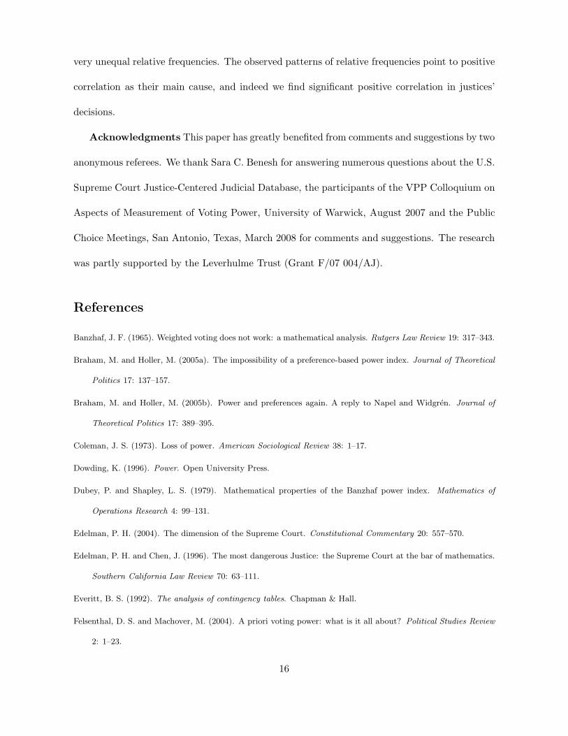
Table 1 gives an example illustrating the above calculation for a weighted voting game with

n = 3, q = 4, w1 = 3, w2 = 2 and w3 = 1. The discrepancy between the behavioral and

constitutional power measures is evident in this example.

2.4. Preferences

In seeking to allow for preferences in a power measure, we agree with Braham and Holler

(2005a: 138) that “the basic concept of power as a potential or capacity cannot accommodate

the preferences of the players whose power we are measuring”. But we believe that a power

measure should accommodate the preferences of the players other that the one whose power is

being measured. In this we hope to reconcile the fundamental critique by Braham and Holler

with the counter-argument by Napel and Widgren (2005: 379) that “preferences are needed to

screen outcomes that are possible and can potentially be affected or forced by a given player

from those that are not possible given all players’ strategic efforts to realize their own will”.

We do not model preferences in the way true preference-based measures do. Typically these

measures model preferences as points in a suitably labeled Euclidean space.9 Our measure does

not specify preferences, strategies, informational asymmetries that may influence the distribution

of votes, and yet it fully accounts for the statistical consequences of the preferences conveyed

by the roll-call data on voting. Whether it was differences in preferences, a plot on the part of

9For example, Steunenberg, Schmidtchen and Koboldt (1999), or Napel and Widgren (2004).

9

other voters, or a basic lack of information that caused this distribution may be important to

the voter, but has no bearing on the measurement of voting power. We therefore do not call

our measure preference-based, but rather empirically informed. Since our measure is based on

the probability space of the classic Penrose-Banzhaf-Coleman measures, it cannot be compared

directly to measures based on a spatial representation of preferences as they have different spaces

of elementary outcomes, and hence also different probability spaces.

3. Voting power in the U.S. Supreme Court

The U.S. Supreme Court is the highest judicial authority of the United States. The Court

comprises the Chief Justice and eight Associate Justices. The justices are nominated by the

President and appointed with the advice and consent of the Senate to serve for life.

The Court votes under simple majority rule provided at least six justices are present for

the Court to be in session. Justices vote in the order of their seniority, starting with the Chief

Justice. Although the Chief Justice has a number of exclusive prerogatives and responsibilities,

all justices have equal a priori voting power.

It is customary to refer to the Court by the name of the presiding Chief Justice, who usually is

the longest-serving member of the Court. We define a bench as a Court in which the same group

of persons sit as justices, and study three benches from the Chief Justice Warren (1953-1969),

Burger (1969-1986) and Rehnquist’s (1989-2005) eras.

3.1. The data

The Supreme Court Justice-Centered Judicial Databases sponsored by the University of Ken-

tucky and maintained by Benesh and Spaeth is a comprehensive source of data on the decisions

10

and opinions of individual justices during the three eras.10

Several decisions had to be made when preparing the data. Our focus is on the relative

frequencies of divisions. For a meaningful analysis we therefore confine the analysis to cases in

which the same bench of justices voted. Out of 228 observed benches we chose the three which

had the largest number of cases, one for each era. The high number of different benches arises

from the combinations of six to nine justices possibly attending a session, and from the fact that

associate justices retired and were replaced in the same era. Our selection includes 416, 1110,

and 683 cases from respectively the Warren, Burger and Rehnquist eras, with all nine justices

voting on each case. Since we would like the cases to be as independent from each other as

possible, we exclude those with multiple legal issues or multiple legal provisions. Finally, we

define a Yes vote as one in favor of the petitioning party.11

3.2. Relative frequencies of divisions

Figure 1 shows the relative frequencies of divisions. With nine justices there will be 512 possible

divisions. The abscissa scale shows the divisions ordered from a unanimous vote against the

petitioning party to a unanimous vote in favor of the petitioning party. Note that:

(i) only a small minority of possible divisions actually has occurred, the percentage in each

bench being Warren (9.4), Burger (31.6) and Rehnquist (21.5);

(ii) the relative frequencies of those which are observed are very unequal;

(iii) unanimity is by far the most common of all voting profiles. The Burger bench is an excep-

tion with the 2:7 divisions against the petitioning party occurring slightly more frequently

than the 0:9 divisions;

10These data are available at http://www.cas.sc.edu/poli/juri/sctdata.htm.11In terms of the variables in the Benesh and Speath databases, we restrict ANALU = 0, delete the duplicate

LED numbers and compute a vote variable which takes the value 1 ifMAJ MIN = WIN DUM , and 0 otherwise.

11

(iv) a unanimous vote in favor of the petitioning party is more frequent than a unanimous

vote against the petitioning party. This suggests a selection bias in the data in favor of

petitions with a reasonable chance of success.

These observations refute the binomial model of equally probable and independent votes as an

empirical description. Although comprehensive voting records such as that for the U.S. Supreme

Court are scarce, data on several other voting bodies reveal that divisions typically occur with

very different frequencies. This is true of the Supreme Court of Canada (Heard and Swartz 1998),

the European Union Council of Ministers (Hayes-Renshaw, van Aken and Wallace 2006) and the

institutions of the United Nations (Newcombe, Ross and Newcombe 1970). In the next section

we show that positive correlations between votes are the primary cause of the observed pattern.

3.3. The behavioral power index

In a voting game with equal weights all voters have equal a priori powers. Under simple-majority

rule with an odd number of votes the Banzhaf absolute measure equals the binomial probability

of (n − 1)/2 successes in n − 1 trials with 0.5 as the probability of success. For n = 9 this

probability equals 0.273.

Table 2 reports the behavioral power index αi for each justice. It is evident that the justices’

behavioral powers are not equal. We quantify this inequality by comparing the Gini coefficient

of αi. The largest inequality is observed in the Warren bench, followed by Rehnquist and

Burger. The biggest losers in terms of behavioral versus a priori voting power were justices

Black, Douglas and Clark of the Warren bench. None of the justices had more behavioral power

than a priori power.

The actual distribution of voting power in the U.S. Supreme Court has been studied be-

fore. Edelman and Chen (1996) compute what essentially is a generalization of the normalized

12

Banzhaf measure of voting power, in which a devision is defined by the group of justices who

join the Court’s opinion. They identify Justice Kennedy as the one who wielded the most voting

power during this period of time. This conclusion is not supported by our calculations for the

Rehnquist bench. We find that it was Justice Souter who had the most power. The difference

can be explained by three facts. First, Edelman and Chen (1996) based their calculations on a

subsample of the data we used, covering the Court’s 1994 and 1995 October Terms only. Sec-

ond, their calculations account for the Court opinions joined by the Justices. Opinions and votes

differ occasionally. A justice may vote with the majority and yet write a dissenting opinion.

Defining divisions based on opinions in the context of a binary choice is also problematic because

the Court may deliver more than two opinions (‘seriatim opinion’). And third, Edelman and

Chen’s measure differs conceptually in that it is not free from the effect of the own vote on the

collective outcome.

4. Coleman’s measure of dependence

The fact that unanimity is by far the most frequent of all divisions points to a positive correlation

between the justices’ votes. The correlation coefficient is a pairwise measure of linear dependence.

But is there a measure of the overall dependence between votes? One such measure has been

proposed in Coleman (1973).

Under the binomial model the variance of the fraction of Yes votes is σ2 = p(1−p)/n, where

p is the probability of a Yes vote, here common to all voters. The sample variance s2 will differ

systematically from σ2 if the assumptions of the binomial model are not met. This will be the

case if votes are not independent, or if the true probability is not p, or both. For example,

if each pair of votes correlates with the correlation coefficients c, then s2 ≈ σ2[1 + (n − 1)c],

13

provided (1−n)−1 ≤ c ≤ 1. The equality is only approximate since s2 depends on the sample of

voting data, i.e., is a statistic. Assuming that the true probability is indeed p, the ratio σ2/s2

is a rough measure of the overall dependence in a voting body of size n.

Coleman used this fact to compute the equivalent number of independent voters m. Setting

s2 = p(1− p)/m yields m = p(1− p)/s2. For independent voters s2 ≈ p(1− p)/n so that m ≈ n.

Compared to n = 9, low values of m for the Warren (1.48), Burger (2.21) and Rehnquist (1.79)

benches suggest a high positive correlations between votes.

A measure of the overall dependence similar to Coleman’s has been proposed in Sirovich

(2003). Sirovich claims that the second Rehnquist U.S. Supreme Court “acts as if composed

of 4.68 ideal Justices”. His measure is based on the concept of informational entropy and is

computed for a sub-sample of the data for the Rehnquist bench analyzed in this paper. We find

an even lower equivalent number of independent Justices on the Rehnquist bench.12

Coleman’s is a measure of the overall dependence. Table 3 reports estimates of the individual

marginal probabilities and correlation coefficients. They show that in most cases the probability

of a Yes vote is not far from 0.5 but that votes are highly positively correlated. For the three

Courts the average probabilities of a Yes vote are 0.63, 0.47 and 0.54. The spreads of the

estimated probabilities range from (0.44, 0.73) for the Warren bench to (0.53, 0.55) for the

Rehnquist bench. The average correlation coefficients between two Yes votes for the three

benches are 0.67, 0.39 and 0.5.

Fisher’s Exact Test13 cannot reject the null hypothesis of conditional independence at the

5% level of significance for only 7 of 108 pairs of justices indicated by an asterisk. There is

significant positive correlation in justices’ decisions.

12For a critique of the equivalent number of independent (or, as Sirovich calls them, “platonic” justices), see acommentary by Edelman (2004).

13See Everitt (1992).

14

One consequence of high positive correlations is that voters often see their preferred outcome

prevail. Several authors have proposed to measure voting power using this probability (Satisfac-

tion index by Straffin (1978), EPW index by Morriss (2002)). We believe that the probability

of being on the winning side is not a valid measure of power because it does not distinguish

between power and luck.14 For example, it assigns power to a voter who cannot swing in any

theoretically conceivable division of votes, a dummy. Our approach is to define power in terms

of the capacity to affect a decision, based on the concept of a swing.

5. Summary

The standard approach to measuring the voting power of a particular member of the voting

body is to compute the probability of her casting a decisive vote. This analysis must encompass

both the formal rules of the voting body and also the behavior of all the voters. The member

is more powerful the more frequently her vote is decisive. But this will depend in practice on

circumstances created by others casting their votes so that she has opportunities to be decisive.

Thus an empirical voting power measure must be based on the frequencies with which the various

voting profiles occur. As is well known, the Penrose-Banzhaf measure ignores behavior and takes

into account only power deriving from the rules construed in a purely formal, a priori sense.

We propose an empirically informed power measure by relaxing this very strong assumption

and replacing it by the use of information about real or assumed voting patterns. The behavioral

power index is based on the probability distribution of divisions of all other voters except the

one whose power is being measured, which can be assumed or estimated using ballot data.

The voting behavior of justices in the U.S. Supreme Court clearly contradicts the assumptions

of equally probable and independent votes. Over a range of cases, voting profiles occur with

14This point has been extensively discussed by Dowding (1996).

15

very unequal relative frequencies. The observed patterns of relative frequencies point to positive

correlation as their main cause, and indeed we find significant positive correlation in justices’

decisions.

Acknowledgments This paper has greatly benefited from comments and suggestions by two

anonymous referees. We thank Sara C. Benesh for answering numerous questions about the U.S.

Supreme Court Justice-Centered Judicial Database, the participants of the VPP Colloquium on

Aspects of Measurement of Voting Power, University of Warwick, August 2007 and the Public

Choice Meetings, San Antonio, Texas, March 2008 for comments and suggestions. The research

was partly supported by the Leverhulme Trust (Grant F/07 004/AJ).

References

Banzhaf, J. F. (1965). Weighted voting does not work: a mathematical analysis. Rutgers Law Review 19: 317–343.

Braham, M. and Holler, M. (2005a). The impossibility of a preference-based power index. Journal of Theoretical

Politics 17: 137–157.

Braham, M. and Holler, M. (2005b). Power and preferences again. A reply to Napel and Widgren. Journal of

Theoretical Politics 17: 389–395.

Coleman, J. S. (1973). Loss of power. American Sociological Review 38: 1–17.

Dowding, K. (1996). Power. Open University Press.

Dubey, P. and Shapley, L. S. (1979). Mathematical properties of the Banzhaf power index. Mathematics of

Operations Research 4: 99–131.

Edelman, P. H. (2004). The dimension of the Supreme Court. Constitutional Commentary 20: 557–570.

Edelman, P. H. and Chen, J. (1996). The most dangerous Justice: the Supreme Court at the bar of mathematics.

Southern California Law Review 70: 63–111.

Everitt, B. S. (1992). The analysis of contingency tables. Chapman & Hall.

Felsenthal, D. S. and Machover, M. (2004). A priori voting power: what is it all about? Political Studies Review

2: 1–23.

16

Garrett, G. and Tsebelis, G. (1999). Why resist the temptation of power indices in the European Union? Journal

of Theoretical Politics 11: 291–308.

Gelman, A., Katz, J. N., and Bafumi, J. (2004). Standard voting power indices don’t work: an empirical analysis.

British Journal of Political Science 34: 657–674.

Hayes-Renshaw, F., van Aken, W., and Wallace, H. (2006). When and why the EU council of ministers votes

explicitly. Journal of Common Market Studies 44: 161–194.

Heard, A. and Swartz, T. (1998). Empirical Banzhaf indices. Public Choice 97: 701–707.

Laruelle, A. and Valenciano, F. (2005). Assessing success and decisiveness in voting situations. Social Choice and

Welfare 24: 171–197.

Morriss, P. (2002). Power: a philosophical analysis. Manchester University Press.

Napel, S. and Widgren, M. (2004). Power measurement as sensitivity analysis: a unified approach. Journal of

Theoretical Politics 16: 517 – 538.

Napel, S. and Widgren, M. (2005). The possibility of a preference-based power index. Journal of Theoretical

Politics 17: 377–387.

Newcombe, H., Ross, M., and Newcombe, A. G. (1970). United Nations voting patterns. International Organiza-

tion 24: 100–121.

Penrose, L. S. (1946). The elementary statistics of majority voting. Journal of Royal Statistical Society 109:

53–57.

Sirovich, L. (2003). A pattern analysis of the Second Rehnquist US Supreme Court. Proceedings of the National

Academy of Sciences of the United States of America 100: 7432–7437.

Steunenberg, B., Schmidtchen, D., and Koboldt, C. (1999). Strategic power in the European Union: evaluating

the distribution of power in policy games. Journal of Theoretical Politics 11: 339–366.

Straffin, P. D. (1978). Probability models for power indices. In P. C. Ordeshook (Ed.), Game Theory and Political

Science. New York University Press.

17

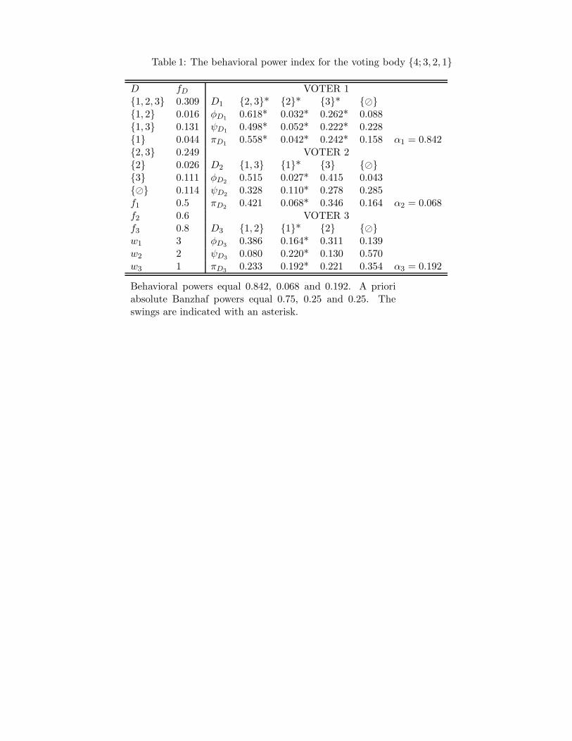
Table 1: The behavioral power index for the voting body {4; 3, 2, 1}

D fD VOTER 1{1, 2, 3} 0.309 D1 {2, 3}* {2}* {3}* {⊘}{1, 2} 0.016 φD1

0.618* 0.032* 0.262* 0.088{1, 3} 0.131 ψD1

0.498* 0.052* 0.222* 0.228{1} 0.044 πD1

0.558* 0.042* 0.242* 0.158 α1 = 0.842{2, 3} 0.249 VOTER 2{2} 0.026 D2 {1, 3} {1}* {3} {⊘}{3} 0.111 φD2

0.515 0.027* 0.415 0.043{⊘} 0.114 ψD2

0.328 0.110* 0.278 0.285f1 0.5 πD2

0.421 0.068* 0.346 0.164 α2 = 0.068f2 0.6 VOTER 3f3 0.8 D3 {1, 2} {1}* {2} {⊘}w1 3 φD3

0.386 0.164* 0.311 0.139w2 2 ψD3

0.080 0.220* 0.130 0.570w3 1 πD3

0.233 0.192* 0.221 0.354 α3 = 0.192

Behavioral powers equal 0.842, 0.068 and 0.192. A prioriabsolute Banzhaf powers equal 0.75, 0.25 and 0.25. Theswings are indicated with an asterisk.

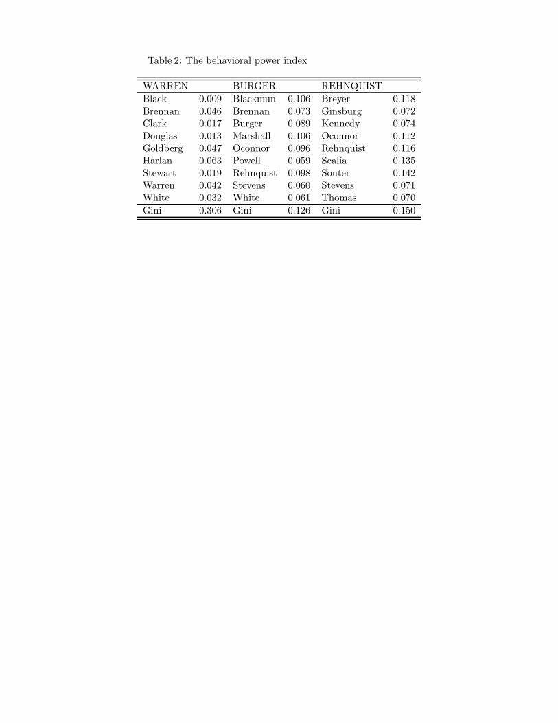
Table 2: The behavioral power index

WARREN BURGER REHNQUIST

Black 0.009 Blackmun 0.106 Breyer 0.118Brennan 0.046 Brennan 0.073 Ginsburg 0.072Clark 0.017 Burger 0.089 Kennedy 0.074Douglas 0.013 Marshall 0.106 Oconnor 0.112Goldberg 0.047 Oconnor 0.096 Rehnquist 0.116Harlan 0.063 Powell 0.059 Scalia 0.135Stewart 0.019 Rehnquist 0.098 Souter 0.142Warren 0.042 Stevens 0.060 Stevens 0.071White 0.032 White 0.061 Thomas 0.070

Gini 0.306 Gini 0.126 Gini 0.150

Table 3: Marginal probabilities and correlation coefficients

WARREN BURGER REHNQUIST(i, j) pi pj ci,j (i, j) pi pj ci,j (i, j) pi pj ci,jBlack-Brennan 0.64 0.73 0.80 Blackmun-Brennan 0.44 0.51 0.36 Breyer-Ginsburg 0.55 0.53 0.72Black-Clark 0.64 0.58 0.56 Blackmun-Burger 0.44 0.49 0.47 Breyer-Kennedy 0.55 0.55 0.48Black-Douglas 0.64 0.65 0.74 Blackmun-Marshall 0.44 0.49 0.35 Breyer-O’Connor 0.55 0.55 0.54Black-Goldberg 0.64 0.70 0.77 Blackmun-O’Connor 0.44 0.47 0.49 Breyer-Rehnquist 0.55 0.54 0.38Black-Harlan 0.64 0.44 0.37 Blackmun-Powell 0.44 0.46 0.54 Breyer-Scalia 0.55 0.55 0.27Black-Stewart 0.64 0.57 0.55 Blackmun-Rehnquist 0.44 0.50 0.37 Breyer-Souter 0.55 0.53 0.71Black-Warren 0.64 0.72 0.79 Blackmun-Stevens 0.44 0.38 0.52 Breyer-Stevens 0.55 0.53 0.58Black-White 0.64 0.64 0.69 Blackmun-White 0.44 0.54 0.46 Breyer-Thomas 0.55 0.55 0.24Brennan-Clark 0.73 0.58 0.67 Brennan-Burger 0.51 0.49 0.00* Ginsburg-Kennedy 0.53 0.55 0.52Brennan-Douglas 0.73 0.65 0.82 Brennan-Marshall 0.51 0.49 0.81 Ginsburg-O’Connor 0.53 0.55 0.50Brennan-Goldberg 0.73 0.70 0.90 Brennan-O’Connor 0.51 0.47 0.05* Ginsburg-Rehnquist 0.53 0.54 0.41Brennan-Harlan 0.73 0.44 0.51 Brennan-Powell 0.51 0.46 0.13 Ginsburg-Scalia 0.53 0.55 0.30Brennan-Stewart 0.73 0.57 0.67 Brennan-Rehnquist 0.51 0.50 -0.10 Ginsburg-Souter 0.53 0.53 0.79Brennan-Warren 0.73 0.72 0.95 Brennan-Stevens 0.51 0.38 0.36 Ginsburg-Stevens 0.53 0.53 0.62Brennan-White 0.73 0.64 0.78 Brennan-White 0.51 0.54 0.12 Ginsburg-Thomas 0.53 0.55 0.27Clark-Douglas 0.58 0.65 0.56 Burger-Marshall 0.49 0.49 -0.03* Kennedy-O’Connor 0.55 0.55 0.72Clark-Goldberg 0.58 0.70 0.59 Burger-O’Connor 0.49 0.47 0.76 Kennedy-Rehnquist 0.55 0.54 0.75Clark-Harlan 0.58 0.44 0.62 Burger-Powell 0.49 0.46 0.73 Kennedy-Scalia 0.55 0.55 0.65Clark-Stewart 0.58 0.57 0.62 Burger-Rehnquist 0.49 0.50 0.75 Kennedy-Souter 0.55 0.53 0.57Clark-Warren 0.58 0.72 0.66 Burger-Stevens 0.49 0.38 0.40 Kennedy-Stevens 0.55 0.53 0.3Clark-White 0.58 0.64 0.69 Burger-White 0.49 0.54 0.59 Kennedy-Thomas 0.55 0.55 0.63Douglas-Goldberg 0.65 0.70 0.77 Marshall-O’Connor 0.49 0.47 0.02* O’Connor-Rehnquist 0.55 0.54 0.71Douglas-Harlan 0.65 0.44 0.34 Marshall-Powell 0.49 0.46 0.10 O’Connor-Scalia 0.55 0.55 0.63Douglas-Stewart 0.65 0.57 0.52 Marshall-Rehnquist 0.49 0.50 -0.13 O’Connor-Souter 0.55 0.53 0.58Douglas-Warren 0.65 0.72 0.83 Marshall-Stevens 0.49 0.38 0.33 O’Connor-Stevens 0.55 0.53 0.25Douglas-White 0.65 0.64 0.63 Marshall-White 0.49 0.54 0.05* O’Connor-Thomas 0.55 0.55 0.64Goldberg-Harlan 0.70 0.44 0.49 O’Connor-Powell 0.47 0.46 0.72 Rehnquist-Scalia 0.54 0.55 0.76Goldberg-Stewart 0.70 0.57 0.66 O’Connor-Rehnquist 0.47 0.50 0.75 Rehnquist-Souter 0.54 0.53 0.45Goldberg-Warren 0.70 0.72 0.89 O’Connor-Stevens 0.47 0.38 0.46 Rehnquist-Stevens 0.54 0.53 0.12Goldberg-White 0.70 0.64 0.69 O’Connor-White 0.47 0.54 0.53 Rehnquist-Thomas 0.54 0.55 0.75Harlan-Stewart 0.44 0.57 0.65 Powell-Rehnquist 0.46 0.50 0.67 Scalia-Souter 0.55 0.53 0.37Harlan-Warren 0.44 0.72 0.48 Powell-Stevens 0.46 0.38 0.47 Scalia-Stevens 0.55 0.53 0.05Harlan-White 0.44 0.64 0.63 Powell-White 0.46 0.54 0.58 Scalia-Thomas 0.55 0.55 0.87Stewart-Warren 0.57 0.72 0.63 Rehnquist-Stevens 0.50 0.38 0.35 Souter-Stevens 0.53 0.53 0.58Stewart-White 0.57 0.64 0.70 Rehnquist-White 0.50 0.54 0.50 Souter-Thomas 0.53 0.55 0.35Warren-White 0.72 0.64 0.74 Stevens-White 0.38 0.54 0.34 Stevens-Thomas 0.53 0.55 0.03

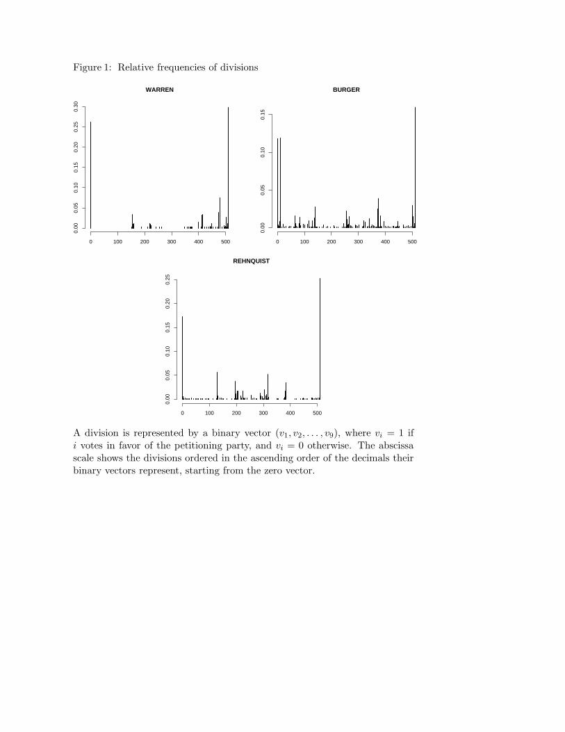
Figure 1: Relative frequencies of divisions

0 100 200 300 400 500

0.00

0.05

0.10

0.15

0.20

0.25

0.30

WARREN

0 100 200 300 400 500

0.00

0.05

0.10

0.15

BURGER

0 100 200 300 400 500

0.00

0.05

0.10

0.15

0.20

0.25

REHNQUIST

A division is represented by a binary vector (v1, v2, . . . , v9), where vi = 1 ifi votes in favor of the petitioning party, and vi = 0 otherwise. The abscissascale shows the divisions ordered in the ascending order of the decimals theirbinary vectors represent, starting from the zero vector.