ECONOMETRICS PRELIM EXAM

August 24, 2010

Department of Economics, Michigan State University

Instructions: Answer all four (4) questions. Be sure to show your work or provide su¢ cient

justi�cation for your answers. Unless explicitly asked, do not worry about regularity conditions such

as existence of moments or di¤erentiability in parameters. This exam is closed book. You may use

a calculator and tables of relevant distributions are provided on additional pages of the exam.

1.(25 points) Let fXng denote a sequence of random variables. Xn is said to converge to X

in mean square if limn!1E[(Xn � X)2] = 0. Xn is said to converge to X in probability if

limn!1 P (jXn �Xj > �) = 0 for any � > 0. It is well known that if Xn converges to X in mean

square then it follows that Xn converges to X in probability.

Let y1; y2; :::yn be a random sample from a population with mean � and variance �2. Assume

that �2 <1. Let y denote the sample average of the y data.

a) Derive formulas for E(y) and var(y):

b) Is y an unbiased estimator of �? Is y a consistent estimator of �? Provide sketches of proofs

for your answers.

De�ne an alternative estimator of � as

e� = y +Xn

where Xn is a discrete random variable de�ned as

Xn = n with probability n�1

Xn = 0 with probability 1� 2n�1

Xn = �n with probability n�1:

Assume that Xn is independent of the y data and assume that n > 1.

c) Derive formulas for E(e�) and var(e�):d) Is e� an unbiased estimator of �? Is e� a consistent estimator of �? Provide sketches of proofsfor your answers.

e) Which is the better estimator of �? Clearly explain what you mean by "better".

1

2. (25 points) Consider the following two regressions:

(1) log(wage) = �0 + �1jc+ �2univ + �3exper + u;

(2) log(wage) = �0 + �1jc+ �2(jc+ univ) + �3exper + u;

where wage is hourly wage, jc is the number of years spent in junior college (2 year college), univ is

the number of years spent at university (4 year college) and exper is years of experience.

Let b� =266664b�0b�1b�2b�3

377775 denote the OLS estimator from regression (1).

Let e =266664e�0e�1e�2e�3

377775 denote the OLS estimator from regression (2).

a) Provide an economic interpretation of the parameters �1 and �2 in regression (2).

b) Prove that e�1 = b�1 � b�2.c) Prove that the SSR (sum of squared residuals) and R2 are the same for regressions (1) and

(2).

d) Prove that se(e�1) = se(b�1 � b�2).e) Prove that the t-statistic for testing H0 : �1 � �2 in regression (1) is exactly equal to the

t-statistic for testing H0 : �1 � 0 in regression (2).

Hint: Determine the 4 � 4 matrix of numbers, G; such that Z = XG where Z is the matrix

of regressors from regression (2) (1; jc; jc + univ; exp er) and X is the matrix of regressors from

regression (1) (1; jc; univ; exp er).

2

3. (25 points) You have used ordinary least squares (OLS) to estimate the housing demand function

logHi = �0 + �1 logPi + �2 log Yi + �3Di + ui

where Hi is the ith family�s units of housing consumption, Pi is their unit price of housing, Yi is their

income, and Di is a dummy variable equal to 1 if they live in an urban area and 0 if not. Based on

404 observations, your estimated equation is

log bHi = 10:0 �:7 logPi +:9 log Yi �:1Di

(1:0) (:3) (:3) (:1)

with R2 = :25. The numbers in parentheses are estimated standard errors, and Cbov(b�1; b�2) = �:085.Assume that the ideal conditions pertain.

a) Brie�y interpret your estimates of �1, �2 and �3:

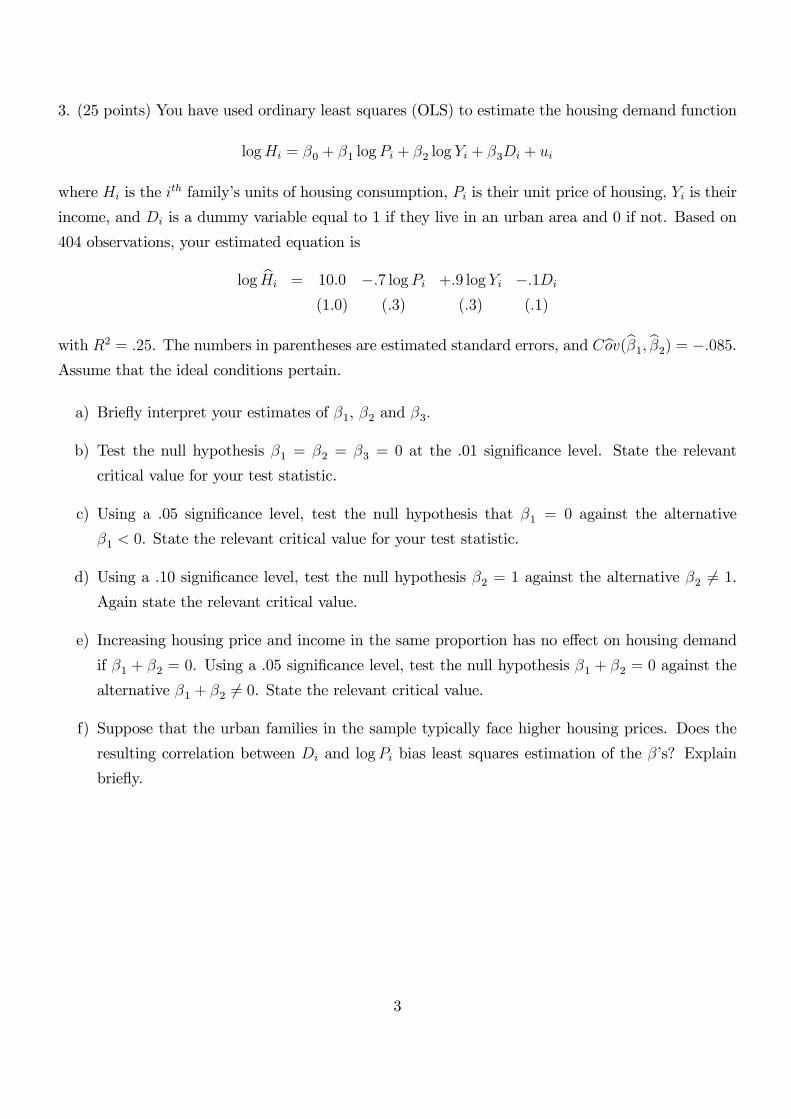
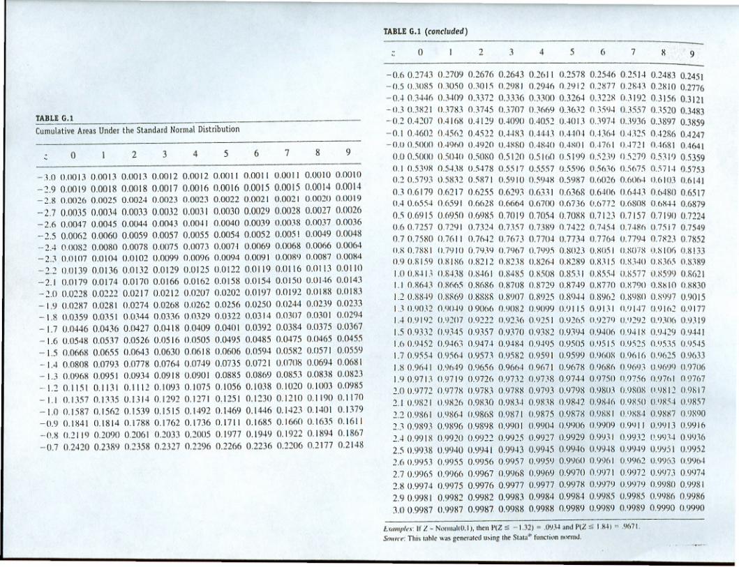
b) Test the null hypothesis �1 = �2 = �3 = 0 at the .01 signi�cance level. State the relevant

critical value for your test statistic.

c) Using a .05 signi�cance level, test the null hypothesis that �1 = 0 against the alternative

�1 < 0. State the relevant critical value for your test statistic.

d) Using a .10 signi�cance level, test the null hypothesis �2 = 1 against the alternative �2 6= 1.Again state the relevant critical value.

e) Increasing housing price and income in the same proportion has no e¤ect on housing demand

if �1 + �2 = 0. Using a .05 signi�cance level, test the null hypothesis �1 + �2 = 0 against the

alternative �1 + �2 6= 0. State the relevant critical value.

f) Suppose that the urban families in the sample typically face higher housing prices. Does the

resulting correlation between Di and logPi bias least squares estimation of the ��s? Explain

brie�y.

3

4. (25 points) Consider the model

Yt = �0 + �1Xt + ��1Xt�1 + �2�1Xt�2 + �

3�1Xt�3 + :::+ ut

where the X�s are exogenous, 0 < � < 1, and ut obeys the ideal conditions. This model represents a

situation in which X has lagged e¤ects on Y , but the lagged e¤ects die out geometrically.

a) At �rst glance this model may seem intractable because it contains an in�nite number of

explanatory variables. This problem can be solved, though, by writing the equation for Yt�1,

multiplying it through by �, and subtracting the resulting equation from the equation for Yt.

Show how this procedure re-expresses Yt as a regression function of only Yt�1 and Xt.

b) Is the regression function from part (a) estimated consistently by OLS? Explain brie�y.

c) Describe an alternative estimation procedure that consistently estimates the coe¢ cients in the

regression of Yt on Yt�1 and Xt.

d) Describe how you would use the resulting coe¢ cient estimates from part (c) to produce con-

sistent estimates of �, �0, and �1.

4