Department of Civil, Surveying and Environmental Engineering The University of Newcastle AUSTRALIA Supervisor:Co-Supervisor: Supervisor:Co-Supervisor:

Department of Civil, Surveying and Environmental EngineeringDepartment of Civil, Surveying and Environmental Engineering

The University of NewcastleThe University of NewcastleAUSTRALIAAUSTRALIA

Supervisor:Supervisor: Co-Supervisor:Co-Supervisor: Garry WillgooseGarry Willgoose Jetse KalmaJetse Kalma

Estimating Soil Moisture Profile Dynamics From Near-Surface

Soil Moisture Measurements and Standard Meteorological Data

Jeffrey WalkerJeffrey Walker

Importance of Soil Moisture Meteorology

Evapotranspiration - partitioning of available energy into sensible and latent heat exchange

Hydrology Rainfall Runoff - infiltration rate; water supply

Agriculture Crop Yield - pre-planting moisture; irrigation

scheduling; insects & diseases; de-nitrification Sediment Transport - runoff producing zones

Climate Studies

Background to Soil Moisture

Remote SensingSatellite

Surface SoilMoisture

Soil MoistureSensors

Logger Soil Moisture Model[q , D ( ), ( )] f s(z)

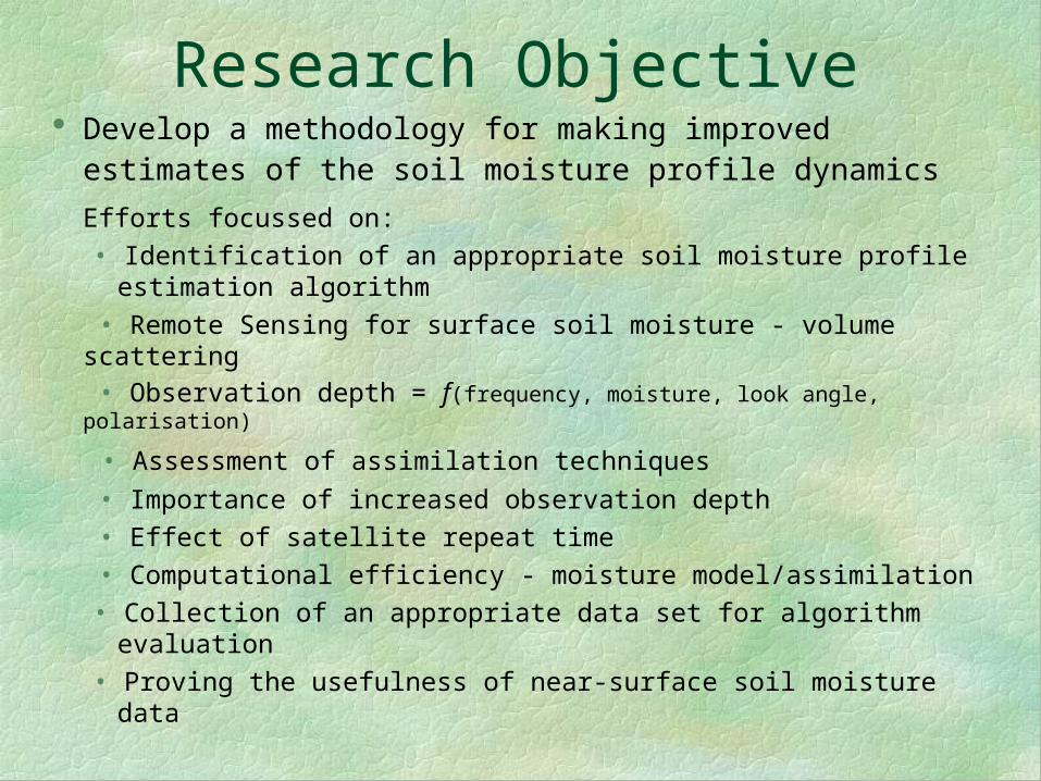
Research Objective Develop a methodology for making improved estimates

of the soil moisture profile dynamics

Efforts focussed on:

• Identification of an appropriate soil moisture profile estimation algorithm

• Remote Sensing for surface soil moisture - volume scattering

• Observation depth = f(frequency, moisture, look angle, polarisation)

• Assessment of assimilation techniques

• Importance of increased observation depth

• Effect of satellite repeat time

• Computational efficiency - moisture model/assimilation

• Collection of an appropriate data set for algorithm evaluation

• Proving the usefulness of near-surface soil moisture data

Seminar Outline Identification of an appropriate methodology for

estimation soil moisture profile dynamics Near-surface soil moisture measurement One-dimensional desktop study Model development

Simplified soil moisture model Simplified covariance estimation

Field applications One-dimensional Three-dimensional

Conclusions and Future direction

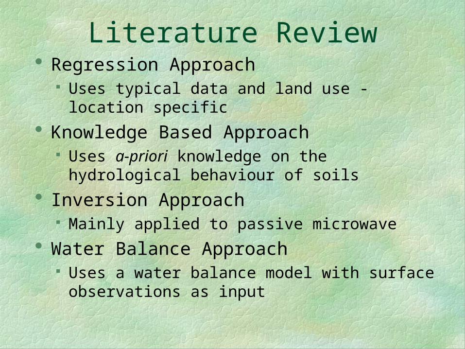
Literature Review Regression Approach

Uses typical data and land use - location specific

Knowledge Based Approach Uses a-priori knowledge on the hydrological

behaviour of soils

Inversion Approach Mainly applied to passive microwave

Water Balance Approach Uses a water balance model with surface

observations as input

Water Balance Approach Updated 2-layer model by direct insertion of

observations - Jackson et al. (1981), Ottle and Vidal-Madjar (1994)

Fixed head boundary condition on 1D Richards eq. - Bernard et al. (1981), Prevot et al. (1984), Bruckler and Witono (1989)

Updated 1D Richards equation with Kalman filter - Entekhabi et al. (1994)

Updated 2-layer basin average model with Kalman filter - Georgakakos and Baumer (1996)

Updated 3-layer TOPLATS model with: direct insertion; statistical correction; Newtonian nudging (Kalman filter); and statistical interpolation - Houser et al. (1998)

Soil Moisture Profile Estimation Algorithm

Initialisation Phase Use a knowledge-based approach

Lapse rate; Hydraulic equilibrium; Root density; Field capacity; Residual soil moisture

Dynamic Phase (Water Balance Model) Forecast soil moisture with meteorological data Update soil moisture forecast with observations

Direct insertion approach Dirichlet boundary condition Kalman filter approach

Matric Head

TrueProfile

ModelPrediction

ModelUpdate

DirectReplacement

WithObservations

Matric Head

Depth

TrueProfile

ModelPrediction

StatisticallyOptimal

Model Update

Data Assimilation

Direct-Insertion Kalman-Filtering

ObservationDepth

The (Extended) Kalman-Filter Forecasting Equations

States: Xn+1 = An X

n + Un

Covariances: n+1 = An n AnT + Q

Observation equationZ = H X + V

1

ψ 2

M

ψ d

⎧

⎨ ⎪

⎩ ⎪

⎫

⎬ ⎪

⎭ ⎪=

1 0 L 0 L 0 0

0 1 L 0 L 0 0

M M O M O M M

0 0 L 1 L 0 0

⎡

⎣

⎢ ⎢ ⎢

⎤

⎦

⎥ ⎥ ⎥

ψ 1

ψ 2

M

ψ d

M

ψ N −1

ψ N

⎧

⎨

⎪ ⎪ ⎪

⎩

⎪ ⎪ ⎪

⎫

⎬

⎪ ⎪ ⎪

⎭

⎪ ⎪ ⎪

+V

Active or Passive? Passive

Measures the naturally emitted radiation from the earth - Brightness Temperature

Resolution - 10’s km 100 km (applicable to GCM’s)

Active Sends out a signal and measures the return -

Backscattering Coefficient More confused by roughness, topography and

vegetation Resolution - 10’s m (applicable to partial area hydrology and

agriculture)

The Modified IEM Modified reflectivities Dielectric profile

m = 12 gives varying profile to depth 3mm Radar observation depth 1/10 1/4 of the

wavelength

0 25

-10

0

10

Dielectric Constant

Depth z (cm)

ε=1

ε=ε∞

=12m=1m

ε

εr z( ) = 1 + ε r∞− 1( )

exp mz( )

1 + exp mz( )

Radar Observation Depth

d

Er=|R|Et´

Evol=|T|Er´

Esur=|R|Ei

Dielectric DiscontinuityDeep Soil Layer

Air Layer

Surface Soil Layer

Ei

Et=|T|Ei Er´=aEr

Et´=aEt

Evol /Esur = ?

Addressed through error analysis of backscattering equation

2% change in mc 0.15 - 1 dB, wet dry Radar calibration 1 - 2 dB 1.5 dB 0.17

Evol

Esur

=∂σ o ln1020

Application of the Models

vv polarisationhh polarisation

rms = 25 mmcorrelation length = 60 mmincidence angle = 23o

moisture content 9% v/v

-20

0

0 5

EMSL dataIEM simulationmodified IEM, transition rate factor=12modified IEM, variable transition rate factor

Backscattering Coefficient (dB)

Frequency (GHz)0 5

Frequency (GHz)

1.5

3.5

hhvv

Observation Depth (cm)

1D Desktop Study 1D soil moisture and heat transfer

C∂∂t

=∇ Dl∇ +Dl[ ]

CT∂T∂t

=∇ λ∇T−cl T −Tref( )ql[ ]

−clρl T −Tref( )∂ l

∂t

Moisture Equation Matric Head form of Richard’s eq. Assumes:

Isothermal conditions (decoupled from temperature)

Vapour flux is negligible

Temperature Equation Function of soil moisture Assumes:

Effect from differential heat of wetting is negligible

Effect from vapour flux is negligible

0

5

10Frequency (GHz)

L S C K Band

0 oC 10 oC 30 oC 50 oC

RealComponent

ImaginaryComponent

1

Temperature Dependence Low Soil Moisture (5%)

0

30

10Frequency (GHz)

L S C K Band

0 oC10 oC

30 oC 50 oC

RealComponent

ImaginaryComponent

1

Microwave remote sensing is a function of dielectric constant

High Soil Moisture (40%)

Synthetic Data

0 10 200

0.5

1

Day

Evaporation (cm/day)

Initial conditions Boundary conditions

0 10 20

-400

0

400

Day

Soil Heat Flux (langley/day)

-600 0-100

0

Matric Head (cm)

PoorInitial

Guess

TrueInitialProfile

0 30-100

0

Soil Temperature (oC)

Depth (cm)

PoorInitial

Guess

TrueInitialProfile

Direct-Insertion Every Hour

Day 1

No Update0 cm

1

4

10 cm

True

Day 3

-600 0-100

0

Matric Head (cm)

Depth (cm)

Day 5 Day 7

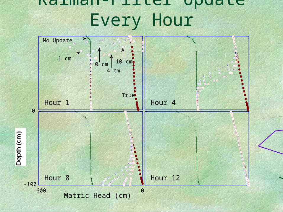
Kalman-Filter Update Every Hour

Hour 1

No Update

0 cm1 cm

4 cm

10 cm

True

Hour 4

-600 0-100

0

Matric Head (cm)

Depth (cm)

Hour 8 Hour 12

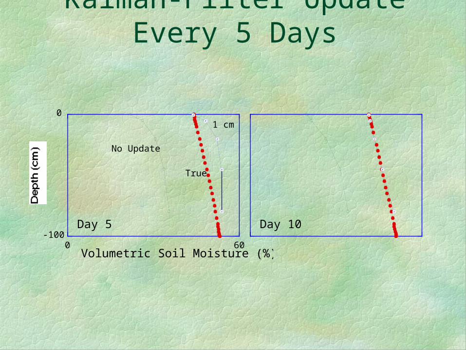
Kalman-Filter Update Every 5 Days

-3000 0-100

0

Matric Head (cm)

Depth (cm)

Day 5

No Update

True

Kalman-FilterUpdate

0Matric Head (cm)

Day 10

No Update

True KalmanFilter

Update

InvalidUpdateRegion

-2000 1000

WaterTable atSurface

Quasi Profile Observations

-600 0-100

0

Matric Head (cm)

Depth (cm)

Model

TrueProfile

Observations

ModelStandardDeviation

SmallStandardDeviation

-600 0Matric Head (cm)

Model

Observations

ModelStandardDeviation

QuasiObservations

QuasiObservation

StandardDeviations

UpdatedProfile

TrueProfile


Day 5

No Update

0 cm

1 cm

4 cm

10 cm

True

-600 0-100

0

Matric Head (cm)

Depth (cm)

Day 10

Day 5

No Update

True

0 cm

0 30Soil Temperature (oC)

Day 10

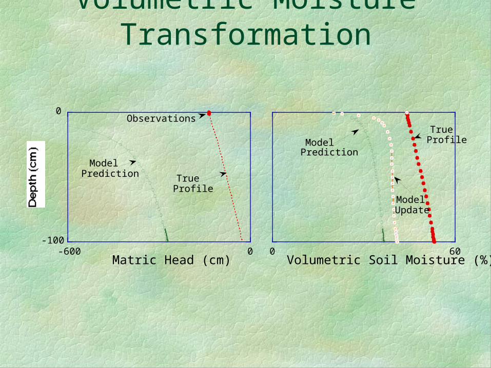
Volumetric Moisture Transformation

-600 0-100

0

Matric Head (cm)

Depth (cm)Model

Prediction

Observations

TrueProfile

0 60Volumetric Soil Moisture (%)

TrueProfileModel

ModelUpdate

Prediction

Summary of Results

Update Direct-Insertion (days) Kalman-Filter (days)

Interval Moisture* Temperature Moisture Temperature

1 Hour 7 − 0.5 2

1 Day >20* >20* 3 6

5 Days >40* >40* 15* 15

Continuous Dirichlet boundary condition Moisture 5 - 8 days Temperature >20 days

10 cm update depth Required Dirichlet boundary condition for 1 hour Required Dirichlet boundary condition for 24 hours Moisture Transformation

A Simplified Moisture Model Computationally efficient -based model

Capillary rise during drying events Gravity drainage during wetting events Lateral redistribution No assumption of water table Amenable to the Kalman-filter

Buckingham Darcy Equationq = K+K

Approximate Buckingham Darcy Equationq = KVDF+Kwhere VDF = Vertical Distribution Factor

Vertical Distribution Factor Special cases

Uniform Infiltration Exfiltration

Proposed VDFVDF =

MGRAD

DZ j+ 12−r( )

2

j − j+1

φ −r

⎛

⎝ ⎜ ⎞

⎠ ⎟

∇ = 0

z

ψ

∇ = ∞

z

ψ

∇ = −∞

z

ψ

Model Comparison Exfiltration (0.5 cm/day)

Infiltration (10 mm/hr)

0 60-100

0

Volumetric Soil Moisture (%)

Depth (cm)

Day 1

0 60-100

0


Depth (cm)

Hour 1

Day 10 Day 25

Hour 12 Hour 24


0 60-100

0


Depth (cm)

Day 5

No Update

1 cm

True

Day 10

KF Modification for 3D Modelling Implicit Scheme

1n+1 Xn+1 + 1

n+1 = 2n Xn + 2

n

State Forecasting

Xn+1 = An Xn + Un

where An = [1n+1]-1 [2

n]

Un = [1n+1]-1 [2

n – 1n+1]

Covariance Forecasting

n+1 = An n AnT + Q

KF Modification for 3D Modelling Covariance Forecast

Auto-regressive smooth of 1 and 2

1n+1 = 1

n + (1 – ) 1

n+1

Estimate correlations from:

= AAT where A = [1]-1 [2]

Reduce to correlation matrix

ρi,j = e where = 1 −

1

Γi,j

a

⎛

⎝ ⎜

⎞

⎠ ⎟b

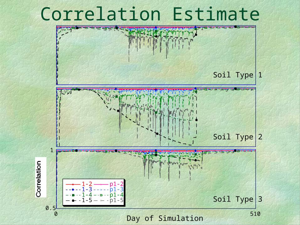
Correlation Estimate

0.5

1

0 510

1-21-31-41-5

p1-2p1-3p1-4p1-5

Correlation

Day of Simulation

Soil Type 3

Soil Type 1

Soil Type 2

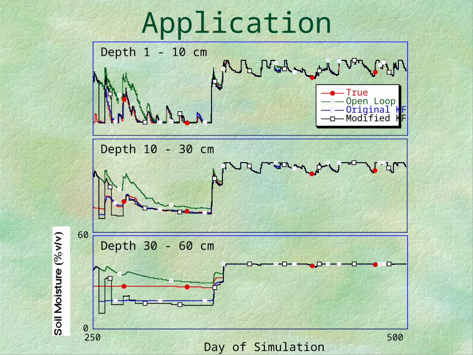
Modified Kalman-Filter Application

0

60

250 500

Soil Moisture (%v/v)

Day of Simulation

Depth 30 - 60 cm

Depth 10 - 30 cm

TrueOpen LoopOriginal KFModified KF

Depth 1 - 10 cm

Field Application

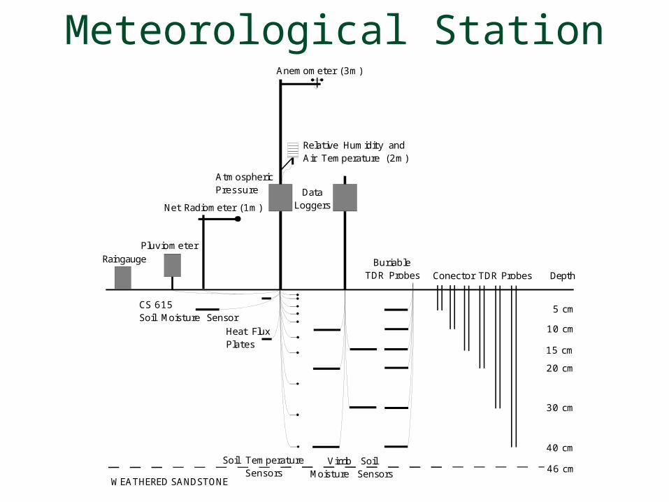
Meteorological Station

CS 615Soil Moisture Sensor

Conector TDR ProbesBuriable

TDR Probes

Net Radiometer (1m)

PluviometerRaingauge

DataLoggers

Relative Humidity andAir Temperature (2m)

Anemometer (3m)

Heat FluxPlates

Soil TemperatureSensors

Virrib SoilMoisture Sensors

Depth

5 cm

10 cm

15 cm

20 cm

30 cm

40 cm

46 cmWEATHERED SANDSTONE

AtmosphericPressure

1D Model Calibration/Evaluation

0

60

May/12 Dec/18 Jul/26


1997 1998

Depth 0-460 mm

Depth 0-235 mm

ModelVirribConnector TDR

Depth 0-123 mm

1D Profile Retrieval - 1/5 Days

0

60

Sep/27 Mar/26 Sep/22


1997 1998

Depth 0-460 mm

Depth 0-225 mm

Open LoopVirribConnector TDRKalman Filter

Depth 0-123 mm

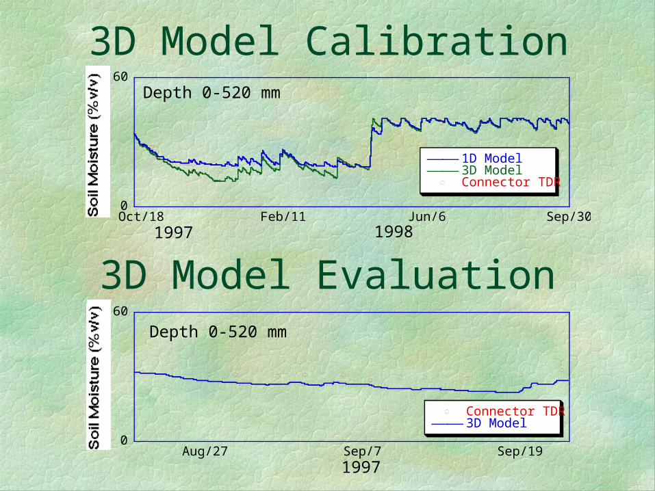
3D Model Calibration

3D Model Evaluation

0

60

Aug/27 Sep/7 Sep/19

Connector TDR3D Model


1997

Depth 0-520 mm

0

60

Oct/18 Feb/11 Jun/6 Sep/30

1D Model3D ModelConnector TDR


1997 1998

Depth 0-520 mm

3D Profile Retrieval All observations

Single Observation

0

60

Aug/27 Sep/7 Sep/19

Connector TDROpen LoopKalman-Filter


1997

Depth 0-520 mm

0

60

Aug/27 Sep/7 Sep/19

Connector TDROpen LoopKalman-Filter


1997

Depth 0-520 mm

Summary of Results

RMS of Horizons for all Profiles (% v/v)Simulation

A1 A1 - A2 A1 - B1 A1 - B2

Evaluation 9.6 5.9 4.6 4.3

Open Loop 20.8 15.8 14.2 13.4

All Observations 9.3 7.9 6.7 6.2

Single Observation 9.4 7.5 6.4 6.1

Conclusions Radar observation depth model has been

developed which gives results comparable to those suggested in literature

Modified IEM backscattering model has been developed to infer the soil moisture profile over the observation depth

Computationally efficient spatially distributed soil moisture forecasting model has been developed

Computationally efficient method for forecasting of the model covariances has been developed

Conclusions Require an assimilation scheme with the

characteristics of the Kalman-filter (ie. a scheme which can potentially alter the entire profile)

Require as linear forecasting model as possible to ensure stable updating with the Kalman-filter (ie. -based model rather than a -based model)

Updating of model is only as good as the models representation of the soil physics

Usefulness of near-surface soil moisture observations for improving the soil moisture estimation has been verified

Future Direction Addition of a root sink term to the simplified soil

moisture forecasting model Improved specification of the forecast system state

variances Application of the soil moisture profile estimation

algorithm with remote sensing observations, published soils and elevation data, and routinely collected met data

Use point measurements to interpret the near-surface soil moisture observations for applying observations to the entire profile - may alleviate the decoupling problem

Documents

Department of Civil, Surveying and Environmental Engineering The University of Newcastle AUSTRALIA Supervisor:Co-Supervisor: Supervisor:Co-Supervisor: