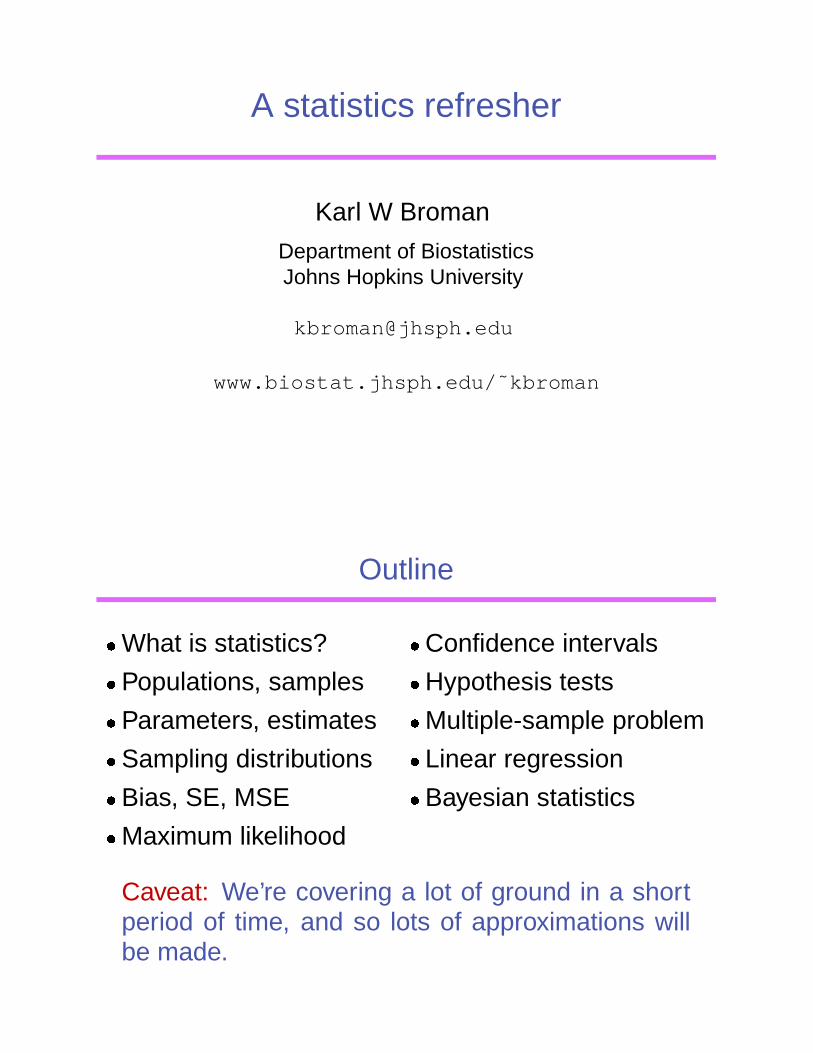
A statistics refresher

Karl W Broman

Department of BiostatisticsJohns Hopkins University

kbroman@jhsph.edu

www.biostat.jhsph.edu/˜kbroman

Outline

� What is statistics?� Populations, samples� Parameters, estimates� Sampling distributions� Bias, SE, MSE� Maximum likelihood

� Confidence intervals� Hypothesis tests� Multiple-sample problem� Linear regression� Bayesian statistics

Caveat: We’re covering a lot of ground in a shortperiod of time, and so lots of approximations willbe made.

We may at once admit that any inference fromthe particular to the general must be attendedwith some degree of uncertainty, but this is not thesame as to admit that such inference cannot beabsolutely rigorous, for the nature and degree ofthe uncertainty may itself be capable of rigorousexpression.

— Sir R. A. Fisher

What is statistics?

� Data exploration and analysis

� Inductive inference with probability

� Quantification of uncertainty

� Experimental design

Populations and samples

We are interested in the distribution of some measurement (ormeasurements) in some underlying (possibly hypothetical) popu-lation (or populations).

Examples: � Infinite number of mice from strain A; cytokine response totreatment.

� All T cells in a person; respond or not to an antigen.

� All possible samples from the Baltimore water supply; concen-tration of cryptospiridium.

� All possible samples of a particular type of cancer tissue; ex-pression of a certain gene.

We can’t see the entire population (whether it is real or hypotheti-cal), but we can see a random sample of the population (perhapsa set of independent, replicated measurements).

Parameters

The object of our interest is the population distribution or, in par-ticular, certain numerical attributes of the population distribution(called parameters).

0 10 20 30 40 50 60

µ

σ

Population distribution Examples:� mean� median� SD� proportion = 1� proportion � 40� geometric mean� 95th percentile

Parameters are usually assigned greek letters (like � , � , and � ).

Sample data

We make n independent measurements (or draw a random sam-ple of size n).

This gives X 1, X 2, . . . , X � , independent and identically distributed(iid), following the population distribution.

Statistic: A numerical summary (function) of the X ’s (that is, of the data).For example, the sample mean, sample SD, etc.

Estimator:(estimate)

A statistic, viewed as estimating some population parameter.

We write:�

� an estimator of ��

p an estimator of p

�

X ��� an estimator of �

S ��� an estimator of �

Parameters, estimators, estimates

� � The population mean� A parameter� A fixed quantity� Unknown, but what we want to know

�

X � The sample mean� An estimator of �� A function of the data (the X ’s)� A random quantity

�x � The observed sample mean

� An estimate of �� A particular realization of the estimator,

�

X� A fixed quantity, but the result of a random process.

Estimators are random variables

Estimators have distributions, means, SDs, etc.

0 10 20 30 40 50 60

µ

σ

Population distribution

� � X 1, X 2, . . . , X 10� �

�

X

3.8 8.0 9.9 13.1 15.5 16.6 22.3 25.4 31.0 40.0 � � 18.6

6.0 10.6 13.8 17.1 20.2 22.5 22.9 28.6 33.1 36.7 � � 21.2

8.1 9.0 9.5 12.2 13.3 20.5 20.8 30.3 31.6 34.6 � � 19.0

4.2 10.3 11.0 13.9 16.5 18.2 18.9 20.4 28.4 34.4 � � 17.6

8.4 15.2 17.1 17.2 21.2 23.0 26.7 28.2 32.8 38.0 � � 22.8

Sampling distribution

0 10 20 30 40 50 60

µ

σ

Population distribution

Sampling distribution depends on:

� The type of statistic

� The population distribution

� The sample size

Distribution of�

X

5 10 15 20 25 30 35 40

n = 5

5 10 15 20 25 30 35 40

n = 10

5 10 15 20 25 30 35 40

n = 25

5 10 15 20 25 30 35 40

n = 100

Bias, SE, RMSE

0 10 20 30 40 50 60

µ

σ

Population distribution

0 5 10 15 20

Dist’n of sample SD (n=10)

Consider�

� , an estimator of the parameter � .

Bias: E� �

� � ��� � E� �

��� � �Standard error (SE): SE

� �

��� � SD� �

��� .RMS error (RMSE): E � � �

� � ��� 2 � � � �bias � 2 � �

SE � 2.

An example

Consider � backcross mice (genotype AA or AB). Let � be thequantitative phenotype of mouse � .Imagine a single gene (QTL) + environmental noise.

Let � � ����� if mouse � is AB/AA at the gene, and suppose there isno segregation distortion, so that Pr

� �� � � � � Pr� � � � � � ����� .

Imagine ����� �� normal�

�����! �#"$� .% � ���&� !� �

��(' � )+*-,/.

0���21 � � �3�4�

� 5 "76Unconditionally, � follows a mixture of normal distributions.% � �8� �

� ����� � % � ����� � � � � � �9��� � % � �:�&� � � �

Example data

Phenotype

80 90 100 110 120 130 140 150

Maximum likelihood

Q: How to estimate ��� , ��� , and � ?

One approach: Use the parameter values for which the data aremost probable.

log likelihood:

� � ��� ��� �3� � ��� Pr�data � ��� ���$ �3�

� ��� �� � ����� ��� � � � ��� �3� � � ����� ��� � ��� ���$ �3���where � � �� � � � �

���� "�� * ,/. ���" ��� ������ �:"!

Maximum likelihood estimates:���� , ���� , � such that

�is maximized.

Fitted curves

Phenotype

80 90 100 110 120 130 140 150

µ̂0 = 101.3

µ̂1 = 120.5

σ̂ = 10.6

Log likelihood surface

90 100 110 120 130 140

90

100

110

120

130

140

µ0

µ 1

A few facts

Let X 1, X 2, . . . , X � be iid with mean = � and SD = � .

Let��

� � � � � � sample mean�

� � � � � ��� � " � � � � � � � sample SD

No matter what: E� �� � � � , SD

� �� � � � � ' � .

E� � " � � � "

If � is large,��

is approximately normally distributed

If the population distribution is normal:�� � normal � " � � � � � � � " � �("� � �� ��

� � � � � � � ' ��� � normal� � � � � ��

� � � � � � � ' ��� � � � � �

Confidence intervals

Suppose we measure the log10 cytokine response in 100 malemice of a certain strain, and find that the sample average (

�x) is

3.52 and sample SD (s) is 1.62.

Our estimate of the SE of the sample mean is 1.62/ ' 100 = 0.162.

A 95% confidence interval for the population mean ( � ) is3.52 � �

2 � 0.16 � = 3.52 � 0.32 = (3.20, 3.84).

What does this mean?

What is the chance that (3.20, 3.84) contains � ?

What is a confidence interval?

A 95% confidence interval is an interval calculated from the datathat in advance has a 95% chance of covering the population pa-rameter.

In advance,�

X � 1.96 � � ' n has a 95% chance of covering � .

Thus, it is called a 95% confidence interval for � .

Note that, after the data is gathered (for instance, n=100,�

X �

3.52, s � 1.62), the interval becomes fixed:�

X � 1.96 � � ' n = 3.52 � 0.32.

We can’t say that there’s a 95% chance that � is in the interval3.52 � 0.32. It either is or it isn’t; we just don’t know.

1 2 3 4 5 6 1 2 3 4 5 6 1 2 3 4 5 6 1 2 3 4 5 6 1 2 3 4 5 6

500 confidence intervals for µ(σ known)

But we don’t know the SD

Use of�

X � 1.96 � � ' n as a 95% confidence interval for � requiresknowledge of � .

That the above is a 95% confidence interval for � is a result of thefollowing:

�

X � �� � ' n

� normal(0,1)

What if we don’t know � ?

We plug in the sample SD (s), but then we need to widen theintervals to account for the uncertainty in s.

The t interval

If X 1 ������ X n are iid normal(mean= � , SD= � ),�

X � t�� � 2 n � 1 � � � ' n is a 1 � � confidence interval for � .

t�� � 2 n � 1 � is the 1 � � � 2 quantile of the t distribution

with n � 1 “degrees of freedom.”

−4 −2 0 2 4t(α 2, n − 1)

α 2

1 2 3 4 5 6 1 2 3 4 5 6 1 2 3 4 5 6 1 2 3 4 5 6 1 2 3 4 5 6

500 BAD confidence intervals for µ(σ unknown)

1 2 3 4 5 6 1 2 3 4 5 6 1 2 3 4 5 6 1 2 3 4 5 6 1 2 3 4 5 6

500 confidence intervals for µ(σ unknown)

Hypothesis testing

85 90 95 100 105 110 115

A

B

Question: Do the two strains have the same mean?

We imagine X 1 ������ X n � iid normal( � � , � � )Y 1 �� ���� Y m � iid normal( ��� , ��� )

H0 � � � � ��� Ha � � ���� ���

Question: Are the data compatible with H0?

Test statistic

In order to determine whether the data are compatible with H0, weform a summary statistic, for which large values indicate evidencefor a departure from the null hypothesis � � � ��� .

The statistic to use depends on

(a) the types of parameters in question

(b) the form of the data

(c) our assumptions about the process generating the data

In the above example, we’d use T =

�

X ��

Y�SD

� �

X ��

Y �Rejection rule: Reject H0 if �T � � , for some “critical value,” .

P-values

� P-values are a function of the data. (They are random, likedata.)

� P-values measure the strength of evidence against H0.(Take this with a grain of salt.)

� Small p-values indicate evidence against H0.� P = probability of getting this sort of extreme data, if the

observed difference were just due to chance variation.� NOT the probability that the observed difference is due to

chance.� Note that P=0.048 is essentially the same as P=0.053.

Permutation test

X or Y groupX 1 1X 2 1... 1

X n 1 � Tobs

Y 1 2Y 2 2... ...

Y m 2

X or Y groupX 1 2X 2 2... 1

X n 2 � T�Y 1 1Y 2 2... ...

Y m 1

Group status shuffled

Compare the observed t-statistic to the distribution obtained byrandomly shuffling the group status of the measurements.

Permutation distribution

−4 −3 −2 −1 0 1 2 3 4 5 6 7

P-value = Pr( �T � � � �Tobs � )Small n: Look at all � �����

� � possible shuffles

Large n: Look at a sample (w/ repl) of 1000 such shuffles

Example

For each of 8 mothers, we observe (estimates of) the number ofcrossovers, genome-wide, in a set of independent meioticproducts.

Question:

Do the mothers vary in the number of crossoversthey deliver?

The data

30 35 40 45 50 55 60

Fam

ily

No. crossovers

102

884

1331

1332

1347

1362

1413

1416

Example (cont.)

How do we think about this?

If there were no relationship between family ID and numberof crossovers in a meiotic product:

� What sort of data would we expect?� What would be the chance of obtaining data as extreme

as what was observed?

Permuted data

30 35 40 45 50 55 60

Fam

ily

No. crossovers

102

884

1331

1332

1347

1362

1413

1416

The F statistic

�groups�# values in group ���� = � th value in � th group

Assume the data are independent, and that ��� � Normal�

� 4 �#"$� .Question: Are the �3 the same?

Let ���� � � � ���� � ��� � �# and ���� � � �� � � � �

��� � ��� � � �� � �#Let SS � � � �� � �# � ���� �

� �� �:" and SS � � � �� � � � ���� � � ��� �

���� �:"�

�SS � � � � � � �

SS � � � � �# � � �

Estimated permutation distribution

0 1 2 3 4 5

F statistic

Fobs

The above example concernsthe analysis of variance (ANOVA)

Another example

Consider � intercross mice.

Let � = phenotype of mouse �Let � �

���� � �� if mouse � isBBABAA

at a marker

Imagine � � normal�

��� � � " �Question: ��� � ��� � � " ?

ANOVA as linear regression

Let �� �

���� � ��� � if � �

� �� and �� �

���� �� �� if � �

� ��Then � � � � � � � �� � normal

� � �#"$�Estimate � , � , by least squares

(equivalent to maximum likelihood here)

RSS � � � � ���!�:" � � � � �

�� ��� � �

� ��!�:"Note: ����� � � � � � � � � � �� � � � � � � �

A sex effect

Let � = 1/0 if mouse � is male/female.

Consider the model: � � � � � �� � �� ��� � � mean phenotype

marker genotype females males

BB � � � � ��� � �

AB � �� � ��� ��AA � � � � ��� � �

A sex effect

5

10

15

20

25

30

AA AB BB

Genotype

Mea

n ph

enot

ype

female

male

Sex by marker interaction

Consider the model: � � � � � � � ��� � ����� � � � � ����� � � � � � mean phenotype

marker genotype females males

BB � � � � ��� � � �����AB � �� � ��� �� ��� �AA � � � � ��� � � � � �

Sex by marker interaction

5

10

15

20

25

30

No interaction

AA AB BB

Genotype

Mea

n ph

enot

ype

female

male

5

10

15

20

25

30

Interaction

AA AB BB

Genotype

Mea

n ph

enot

ype

female

male

An age effect

Let � be the age of mouse � .Consider the model: � � � � � �� � �� ��� � �

marker genotype mean phenotype

BB � � � ��� � AB � �� ��� � AA � � � ��� �

An age effect

50 100 150 200

5

10

15

20

25

30

Age

Mea

n ph

enot

ype

AA

ABBB

Age by marker interaction

Consider the model:� � � � � �� � �� ��� � ��� � � �� � !� ��� � � �� � !� � marker genotype mean phenotype

BB � � � � � � ��� � � � AB � �� � � � ��� � � � AA � � � � � � � � � � �

Age by marker interaction

50 100 150 200

5

10

15

20

25

30

No interaction

Age

Mea

n ph

enot

ype

AA

ABBB

50 100 150 200

5

10

15

20

25

30

Interaction

Age

Mea

n ph

enot

ype

AA

AB

BB

Frequentist statistics

The target is inference regarding some fixedpopulation parameter, � .

We imagine repeating the sampling/measurementprocess.

We focus on the sampling distribution of astatistic/estimator.

Bayesian statistics

Imagine the population parameter, � , is drawn fromsome prior distribution, Pr( � ).

We calculate the distribution of � conditional on theobserved data (the “posterior” distribution)

Pr�

� � � � � Pr� � � ��� Pr

����

All inference follows from careful study of Pr�

��� � � .

Example

Suppose we are interested in the proportion of 8 week old maleC57BL/6J mice that survive some infection.

We infect � = 10 mice and note that � = 3 survive.

Frequentist:��� binomial

�10 �����

A 95% confidence interval for � is 7 – 65%.

In advance, we had a 95% chance that our interval would contain � ; afterthe fact, it either does or doesn’t.

Bayesian:��� binomial

�10 �����

Imagine that � � uniform� ����� , a priori.

There’s a 95% chance that � is in the interval 9–59%.

References

� L Gonick, W Smith (1993) The cartoon guide to statistics. HarperCollins.

� D Freedman, R Pisani, R Purves (1998) Statistics, 3rd edition. Norton.

� JA Rice (1995) Mathematical statistics and data analysis, 2nd edition. Duxbury.

� ML Samuels, JA Witmer (1999) Statistics for the life sciences, 2nd edition.Prentice Hall.

� FL Ramsey, DW Schafer (2002) The statistical sleuth: A course in methods ofdata analysis, 2nd edition. Duxbury.

� PV Rao (1998) Statistical research methods in the life sciences. Duxbury.

� BJF Manly (1997) Randomization, bootstrap and Monte Carlo methods in biol-ogy, 2nd edition. Chapman & Hall/CRC