Department for Environment, Food and Rural Affairs ...sciencesearch.defra.gov.uk/Document.aspx?Document=DefraSP057… · Department for Environment, Food and Rural Affairs Research

Department for Environment, Food and Rural Affairs Research project final report

Project title Climate change impacts on soil biota - development of a resistance and resilience assay

Defra project code SP0570

Contractor organisations

Cranfield University

The Macaulay Institute

Report authors Karl Ritz ([email protected]), Jim Harris, Mark Pawlett, Helaina Black, Clare Cameron

Project start date September 2009

Project end date March 2011

SP0570 Final report ‐ Page 2

Climate change impacts on soil biota - development of a resistance and resilience assay

1. Summary This study aimed to explore the development of a methodology appropriate to assess the likely impacts of climate change upon key soil biological properties. The concept was based upon measuring the ability of certain biological properties of soils to resist climatically-based perturbations (i.e. ‘resistance’) and the extent to which they then recovered following such perturbation (i.e. ‘resilience’). The perturbations were based upon a single cycle of drying and rewetting, or one of flooding and draining. A laboratory-based assay was developed and applied to six soils originating from Sweden, Scotland, England, France, Spain and Greece, representing a latitudinal European gradient. The responses of soil processes relating to C and N cycling, and the soil microbial (phospholipid fatty acid profiling) and were measured. Resistance and resilience phenomena were quantified by a range of indices. In general, soils were less resistant to drying than flooding. This was particularly the case for the microbial community phenotypic profiles, and notably so for the soils derived from the northern and southern extremes of the latitudinal gradient. In relative terms, there was some evidence that the soils from Scotland and England showed least resistance generally. There was also a distinct decrease in resistance to flooding in the microbial phenotypic profiles down the latitudinal gradient, which circumstantially supports the hypothesis that communities in soils from more arid zones are more immediately affected by flooding. In most cases, there was significant temporal variation in properties in the unperturbed (control) soils, which affected interpretation of resilience depending on what was deemed the ‘norm’. It was judged that perturbed soils should be compared with their respective controls at a common time-point. In that case, all soils exhibited a high degree of resilience to both forms of perturbation. The property which showed most suitability as an indicator in this context was microbial phenotypic profiling, providing data that essentially satisfied the criteria of discrimination, sensitivity, ubiquity and interpretability. The resistance and resilience assay shows definite promise in terms of being an effective indicator of climate change impacts upon soil systems. Its further development needs to involve more extensive perturbations and high-throughput systems to accommodate the inherent temporal and spatial variation exhibited by soils.

2. Background and rationale Climate change has been identified as one of the key pressures likely to affect the soils of England and Wales both now and increasingly so in the future. Under current climate projections, UK soils will continue to experience increasingly drier, hotter summers and wetter, milder winters. These climatic changes will ultimately alter the capacity of soils to maintain their functions, and consequently impact on the delivery of ecosystems goods and services which are reliant upon soil properties and processes. Soil flora and fauna have a fundamental role in delivering and regulating many of the soil properties and processes that underpin the delivery of soil functions. Such links between soil biota and soil functioning mean that biological indicators are likely to be of utility to monitor both the status and changes in soil quality. This concept was studied in detail in Defra Project SP0538, which identified a series of basic candidate soil biological indicators (Ritz et al. 2009). In order to test for the impacts of climate change on soil biota, the logical approach is to monitor the biotic status of soils over time in the context of climate-based parameters and interpret changes in the biotic status with respect to the


delivery of key soil functions. This has been the conventional approach largely adopted to date. The principal drawback of this approach is that is based on ‘real time’, and offers little in terms of any pre-emptive indication of consequential changes. We proposed to test and develop a methodology which measures responses of these indicators as a consequence of the application of prescribed and controlled perturbations that are pertinent to climate change scenarios. The rationale here is that such responses are more likely to reflect climate change impacts than properties measured alone outside of the context of a perturbation.

The concept proposed is based upon that of a ‘resistance and resilience’ assay, appropriate to establish the likely effects of climate change on biotically-mediated soil functions. The basic principles of such techniques in the context of soil systems were first established by (Griffiths et al. 2000; 2001), refined by Orwin and Wardle (2004), and are reviewed in Defra Report SP1605. The basis of the concept is that the change in a property of a soil as a result of some form of perturbation is measured, and its subsequent dynamics over time then quantified. The extent of deviation from the initial state is defined as the resistance, and the trajectory of recovery relates to the resilience of the system with respect to the property being considered. This trajectory of recovery is time-dependent, and hence resilience is defined as the extent of recovery at a prescribed time.

A central hypothesis is that soils which have developed under contrasting climatic conditions would respond in contrasting ways to the same climatic perturbations, reflecting regional differences in inherent soil resistance and resilience developed as a result of differing pedogenic processes and regional adaptation by the soil communities.

3. Objectives:

1. To develop a resistance and resilience assay appropriate to assess the impacts of climate change on soil biota

2. To test the methodology by applying it to a suite of six grassland soils sourced from a N-S series across Europe, and deploying a multi-variate range of soil biological indicators

3. To evaluate the appropriateness of the methodologies in terms of discrimination, sensitivity, ubiquity and interpretability

4. To produce recommendations for further development of the methodology, outline its applicability for wider-scale deployment, and where appropriate produce standard operating procedures for the methodology.

4. Approaches 4.1 Soils

Grassland soils from a pan-European gradient were procured from six countries representing a N-S trajectory, viz. Sweden (abbreviated to SWE hereafter), Scotland (SCO), England (ENG), France (FRA), Spain (ESP) and Greece (GRC). These sites were selected to encompass a range of climate scenarios UK soils are likely to be subjected to over the next several decades. Precise locations and basic soil properties are shown in Fig. 1. Grasslands were deemed as the most appropriate land-use for this study since this ecotype was present in all countries, and all classes of biological indicator were notionally represented, and the inherent biodiversity grassland soils tends to relatively high.

Fig. 1: Locations and basic properties of soils used in study.

SCO

ENG

SWE

FRA

ESP GRC9.7

11.0

10.3

11.1

12.6

11.1

C:N

0.12

0.15

0.25

0.18

0.34

0.18

GRC

ESP

FRA

ENG

SCO

SWE

Country code

20

35

28

31

36

35

Silt

1.25.31367Greece

1.76.91055Spain

2.65.51557France

2.05.71356England

4.36.51153Scotland

2.05.41550Sweden

pHClaySandCountry

9.7

11.0

10.3

11.1

12.6

11.1

C:N

0.12

0.15

0.25

0.18

0.34

0.18

%N

GRC

ESP

FRA

ENG

SCO

SWE

Country code

20

35

28

31

36

35

Silt

1.25.31367Greece

1.76.91055Spain

2.65.51557France

2.05.71356England

4.36.51153Scotland

2.05.41550Sweden

%CpHClaySandCountry

SCO

ENG

SWE

FRA

ESP GRC9.7

11.0

10.3

11.1

12.6

11.1

C:N

0.12

0.15

0.25

0.18

0.34

0.18

GRC

ESP

FRA

ENG

SCO

SWE

Country code

20

35

28

31

36

35

Silt

1.25.31367Greece

1.76.91055Spain

2.65.51557France

2.05.71356England

4.36.51153Scotland

2.05.41550Sweden

pHClaySandCountry

9.7

11.0

10.3

11.1

12.6

11.1

C:N

0.12

0.15

0.25

0.18

0.34

0.18

%N

GRC

ESP

FRA

ENG

SCO

SWE

Country code

20

35

28

31

36

35

Silt

1.25.31367Greece

1.76.91055Spain

2.65.51557France

2.05.71356England

4.36.51153Scotland

2.05.41550Sweden

%CpHClaySandCountry


The target soil type was of light sandy-loam texture, prescribed in order to make the experimental system conducive to uniformity, for example with respect to microcosm packing, rapid attainment of target water status’ and homogenisation during assay procedures. Soils were sampled by project partners and transported to Cranfield, where they were stored moist at 4ºC until application of assays.

4.2 Experimental procedure

The assay proposed to be developed was in this case based on rapidly-induced changes in moisture status, deemed appropriate in the context of the climate-change emphasis the assay is targeting. Soils were sieved <2 mm in their moist state, and packed into polypropylene ring microcosms (inner dimensions 70 mm diameter 50 mm height) at a dry bulk density equivalent to 1.1 g cm-3 (Fig. 2). Their field water-holding capacity (WHC) was determined by free draining, and adjusted to 45% of this value. All microcosms were pre-incubated at 20ºC for 10 days in a sealed moist environment to allow preparation effects to recede. One third of the microcosms were then air-dried at 35º for 7 days. Preliminary experiments showed that 95% of drying-induced water loss was attained within 48 h of such treatment. A further one third of the microcosms were flooded by immersion (individually) in water and held in such a state for 5 days at 10ºC. They were then drained to 45% of their WHC within 2 days. All treated cores were then returned to the incubator where the control microcosms had prevailed during these perturbation treatments. Treatments were arranged according to a randomised block design within the incubator. Immediately following rehydration of the dried cores (and hence when the flooded microcosms had attained their target moisture status), three replicates of each of the treatments were taken, for each of the 6 soils (total n= 54), soils were removed and mixed and the following parameters measured on aliquots:

(i) Respiration rate, at 20ºC, at periodic intervals over c. 50 days following the sampling event, by alkaline trapping of CO2 and titration.

(ii) Multiple-substrate induced respiration rate (MSIR) by the Microresp® procedure.

(iii) Potential N mineralisation rate over 72 h following sampling, by a chlorate-block procedure with supplementary ammonium.

(iv) Actual N mineralisation rate over c.50 days following the sampling event, by determining mineral N concentrations following microcosm sampling and after incubation period.

(v) Nematode community structure by wet extraction and microscopic identification.

(vi) Microbial phenotypic community structure by phospholipid fatty-acid (PLFA) profiling.

These parameters were determined according to established methods; the standard operating procedures are given in Appendix I.

This initial sampling time is denote T0 hereafter. A further three replicates of each treatment were subsequently sampled after a further 7, 27 and 84 days following removal of the perturbations, denoted T7, T27 and T84 hereafter. The experimental design is shown schematically in Fig. 3.

3

3

3

• Nmin

• PNR

• LT Resp

• MSIR

• PLFA

• Worms

CON

FLD

DRY

T7

7 days post removal

3

3

3

• Nmin

• PNR

• LT Resp

• MSIR

• PLFA

• Worms

CON

FLD

DRY

3

3

3

• Nmin

• PNR

• LT Resp

• MSIR

• PLFA

• Worms

CON

FLD

DRY

12

12 12

12 12

12

12

Rewet

DrainFlood

Dry

12 3

3

3

• Nmin

• PNR

• LT Resp

• MSIR

• PLFA

• Worms

CON

FLD

DRY

T0

Immediately post removal of perturb’n

FOR EACH SOIL:

Sum = 36 cores per soil

Grand Sum = 216 cores Grand Sum = 54 cores per time

Control

5 days

7 days*

T27

27 days post removal

T84


3

3

3

• Nmin

• PNR

• LT Resp

• MSIR

• PLFA

• Worms

CON

FLD

DRY

T7

7 days post removal

3

3

3

• Nmin

• PNR

• LT Resp

• MSIR

• PLFA

• Worms

CON

FLD

DRY

3

3

3

• Nmin

• PNR

• LT Resp

• MSIR

• PLFA

• Worms

CON

FLD

DRY

12

12 12

12 12

12

12

Rewet

DrainFlood

Dry

12 3

3

3

• Nmin

• PNR

• LT Resp

• MSIR

• PLFA

• Worms

CON

FLD

DRY

T0

Immediately post removal of perturb’n

FOR EACH SOIL:

Sum = 36 cores per soil

Grand Sum = 216 cores Grand Sum = 54 cores per time

Control

5 days

7 days*

T27


T84


Fig. 3. Schematic of experimental design. CON = control; FLD = flooding treatment; DRY = drying treatment. Other abbreviations relate to assays applied: Nmin = N mineralisation; PNR = potential nitrification rate; LT Resp = long‐term respiration; MSIR = multiple substrate induced respiration;PLFA = phospholipid fatty‐acid [profiling].

Fig. 2: Soils packed into microcosms prior to onset of study. Scale bar = 25 mm.

(a) SWE (b) SCO (c) ENG

(f) GRC(e) ESP(d) FRA


4.3 Calculation of resistance and resilience

Resistance and resilience indices were calculated by three basic procedures, providing absolute, relative and bounded measures (Fig. 4). Absolute and relative measures essentially prescribe the control (unperturbed), with which perturbed systems are compared, as that contemporary with the sampling time following the perturbation; bounded measures are scaled between -1 and +1, where a value of +1 denotes total resistance or resilience relative to the control (unperturbed) system at the time the perturbation was deemed removed. For absolute and relative measures, the terms are arranged such that a negative value equates to a reduction in the property relative to the control, and a positive value an increase in value. For activity rates, this is interpretable as an inhibition or stimulation of the associated processes respectively. For univariate data (e.g. N mineralisation rates), the response variables were taken to be the variates themselves.

The dimensionality of multivariate profiles was reduced by principal component analysis (PCA), using the correlation matrix, applied in two modes: (i) to profiles relating to soils sourced from each country independently, which is appropriate to determine resistance and resilience within each such soil; (ii) combining profiles for all soils across all countries, which is appropriate to establish the relative scales of resistance and resilience within and between the soils of different origin.

4.4 Statistical analyses

Data were analysed by factorial analysis of variance (ANOVA), transforming where necessary to ensure normality of the distributions. Where appropriate, Fisher’s multiple-range test was used to determine homogenous groups of means at the 95% level of significance.

5. Results and discussion 5.1 Long-term respiration

Respiration rates were significantly greater in all soils immediately following removal from the microcosms, and consistently showed a decline thereafter (Figs. 5-8). This was particularity the case for soils sampled at T0 (Fig. 5). Inherent (overall mean) soil respiration rates differed significantly between the soils from different origins at T0, T7 and T27, but not at T84 (Figs. 5h - 8h). At T0 and T7, soils from SCO, ENG, FRA and ESP respired at similar rates, with those from SWE and GRC respiring more slowly, and GRC at the lowest relative rate (Figs. 5 and 6). At T27, there was a consistent pattern of respiration rates across the geographical north-south transect, peaking around ENG (Fig. 7g). By T84 respiration rates were so low in all cases that they were bordering on the limit of detection of the assay system adopted (Fig. 8). Mean respiration rates thus generally declined between T0 and T84, which would be expected given that the soils did not receive any supplementary energy inputs whilst incubating in the microcosms, and they were incubated under constant environmental conditions. The drying and flooding perturbations generally had very small effects upon respiration rates within each soil of origin, relative to the control soils, and there were no third-order interactions in the ANOVA (Figs. 5-8). Where there were significant second-order interactions, these showed no distinct trends in relation to perturbation, time, or country of origin. Similarly, where there were main effects of perturbation, these were very modest in absolute terms and are unlikely of any functional significance. It was not possible to prescribe a mathematical function which adequately fitted the time-course curves of respiration in all cases, which would provide an alternative means of globally analysing the respiration data.

Fig. 4. Calculation of resistance and resilience indices, based on hypothetical response curves to perturbation. Forms (3) and (6) according to Orwin and Wardle 2004.

Prop

erty

0

D0

Time

Perturbation Control(not perturbed)

Dx

C0 Cx

Px

P0

Perturbed

t0 tx

100

Prop

erty

0

D0

Time


Dx

C0 Cx

Px

P0

Perturbed

t0 tx

100

Absolute resistance = P0 – C0

Relative resistance (%) = (P0 – C0) / C0 * 100

Bounded resistance = |)D|(

|D|2100

0

+−

C

(1)

(2)

(3)

Absolute resilience = Px – Cx

Relative resilience (%) = (Px – Cx) / Cx * 100

Bounded resilience = 1|)D| |D(|

|D |2

x0

0 −+

(4)

(5)

(6)

n

Prop

erty

0

D0

Time


Dx

C0 Cx

Px

P0

Perturbed

t0 tx

100

Prop

erty

0

D0

Time


Dx

C0 Cx

Px

P0

Perturbed

t0 tx

100




|D|2100

0

+−

C

(1)

(2)

(3)




|D|2100

0

+−

C

(1)

(2)

(3)




|D |2

x0

0 −+

(4)

(5)

(6)




|D |2

x0

0 −+

(4)

(5)

(6)

n

T0(a) SWE (b) SCO (c) ENG

(d) FRA (e) ESP (f) GRC

(g) Country means (h) Perturbation means

Error

**

580509855

p***

***

297

Country*PerturbationCountry*PSI_0_timePerturbation*PSI_0_timeCountry*Perturbation*PSI_0_time

µg C

O2

g-1

day-

1

368

477969082233

MSSourceCountryPerturbationPSI_0_time

0

50

100

150

200

0 10 20 30 40 50

CONDRYFLD

0

50

100

150

200

0 10 20 30 40 500

50

100

150

200

0 10 20 30 40 50

0

50

100

150

200

0 10 20 30 40 50

Time (days)

0

50

100

150

200

0 10 20 30 40 50

Time (days)

0

50

100

150

200

0 10 20 30 40 50

Time (days)

Figure 5. Time‐courses of respiration rates following sampling and associated ANOVA terms for soils sampled zero days following applied perturbations (i.e. T0 in experimental notation). (a) – (f) individual countries [n=3]; (g) means by country, across perturbations [n=63], similar letters denote homogeneous groups; (h) means by perturbation, across countries [n=126]. Points/columns denote means, whiskers denote pooled standard errors. NB all axes scaled to be uniform between Figures 5‐8.

0

20

40

60

80

100

SWE SCO ENG FRA ESP GRC0

25

50

75

100

Control Dry Flood

b ba b b c



(g) Country means (h) Perturbation meansSourceCountryPerturbation

240

4670256716923PSI_7_time

247

Country*PerturbationCountry*PSI_7_timePerturbation*PSI_7_timeCountry*Perturbation*PSI_7_time

425

p*********

MS

µg C

O2

g-1

day-

1

Error

***787218

0

50

100

150

200

0 10 20 30 40 50

CONDRYFLD

0

50

100

150

200

0 10 20 30 40 500

50

100

150

200

0 10 20 30 40 50

0

50

100

150

200

0 10 20 30 40 50

Time (days)

0

50

100

150

200

0 10 20 30 40 50

Time (days)

0

50

100

150

200

0 10 20 30 40 50

Time (days)

0

20

40

60

80

100


25

50

75

100

Control Dry Flood

b ba b b c

Figure 6. Time‐courses of respiration rates following sampling and associated ANOVA terms for soils sampled 7 days following applied perturbations (i.e. T7 in experimental notation). (a) – (f) individual countries [n=3]; (g) means by country, across perturbations [n=63], similar letters denote homogeneous groups; (h) means by perturbation, across countries [n=126]. Points/columns denote means, whiskers denote pooled standard errors. NB all axes scaled to be uniform between Figures 5‐8.



(g) Country means (h) Perturbation meansSourceCountryPerturbation

130

309289315789PSI_27_time

130

Country*PerturbationCountry*PSI_27_timePerturbation*PSI-27-timeCountry*Perturbation*PSI_27_time

183

p********

MS

µg C

O2

g-1

day-

1

Error

13087

0

50

100

150

200

0 10 20 30 40 50

CONDRYFLD

0

50

100

150

200

0 10 20 30 40 500

50

100

150

200

0 10 20 30 40 50

0

50

100

150

200

0 10 20 30 40 50

Time (days)

0

50

100

150

200

0 10 20 30 40 50

Time (days)

0

50

100

150

200

0 10 20 30 40 50

Time (days)

0

20

40

60

80

100


25

50

75

100

Control Dry Flood

d ca b c ab

Figure 7. Time‐courses of respiration rates following sampling and associated ANOVA terms for soils sampled 27 days following applied perturbations (i.e. T27 in experimental notation). (a) – (f) individual countries [n=3]; (g) means by country, across perturbations [n=63], similar letters denote homogeneous groups; (h) means by perturbation, across countries [n=126]. Points/columns denote means, whiskers denote pooled standard errors; note that whiskers often fall within confines of symbols in (a) – (f). NB all axes scaled to be uniform between Figures 5‐8.




Error

**

*

369750

p

***

73

Country*PerturbationCountry*PSI_T84_timePerturbation*PSI_T84_timeCountry*Perturbation*PSI_T84_time

µg C

O2

g-1

day-

1

51

425610447

MSSourceCountryPerturbationPSI_T84_time

0

50

100

150

200

0 10 20 30 40 50

CONDRYFLD

0

50

100

150

200

0 10 20 30 40 500

50

100

150

200

0 10 20 30 40 50

0

50

100

150

200

0 10 20 30 40 50

Time (days)

0

50

100

150

200

0 10 20 30 40 50

Time (days)

0

50

100

150

200

0 10 20 30 40 50

Time (days)

0

20

40

60

80

100


25

50

75

100

Control Dry Flood

a aa a a a

Figure 8. Time‐courses of respiration rates following sampling and associated ANOVA terms for soils sampled 84 days following applied perturbations (i.e. T84 in experimental notation). (a) – (f) individual countries [n=3]; (g) means by country, across perturbations [n=63], similar letters denote homogeneous groups; (h) means by perturbation, across countries [n=126]. Points/columns denote means, whiskers denote pooled standard errors; note that whiskers often fall within confines of symbols in (a) – (f). NB all axes scaled to be uniform between Figures 5‐8.


Given the overall lack of significant differences associated with perturbation, it was considered inappropriate to calculate resistance and resilience parameters. The essential feature of the respiration responses is that rates in all soils were both resistant and resilient to the applied perturbations. Removing the soils from the microcosms represented a secondary physical disturbance, and again the evidence is that recovery (resilience) from such perturbations was also rapid and complete within ten days on all occasions.

5.2 Multiple substrate induced respiration

The MSIR assay proved to be occasionally unreliable and respiratory responses could not be accurately determined due to problems being encountered with the application of the Microresp assay. This was associated with large variation between Microresp colorimetric plates for the blank cells, which are crucial to determine the respiratory profiles. The prescribed coefficient of variation between blank plates should be <5%, however resultant values were of the order of 30% on occasion, for reasons which could not readily be established.

Due to the high error associated with the blanks, the MSIR calculation was inaccurate to the same order of error, and hence was not reliable. Due to the requirement for a coherent dataset over time, it was not possible to determine resistance and resilience parameters for this assay.

5.3 Potential nitrification

Potential nitrification rates varied significantly between countries, with SCO exhibiting an order-of-magnitude greater rates than the other soils (Fig. 9). There was generally a significant temporal variation in PNR in control soils (Fig. 9). PNR was resistant to both forms of perturbation in all soils except SCO and ENG, where the process was significantly reduced by the drying perturbation (Fig.10). All soils were generally resilient with respect to potential nitrification, apart from the ESP and GRC soils with respect to drying, where rates persisted in being significantly greater than their respective controls (Fig. 10). Bounded indices of resistance were consistent with absolute and relative measures, however bounded resilience indices often showed poor association with absolute measures, due to the forced relation with the prevailing rates at T0 (Fig. 10).

5.4 N mineralisation

N mineralisation rates in control soils showed relatively little temporal variation, with the exception of FRA which showed a significant decline over the 84 day incubation period (Fig. 11). There was a distinct pattern of N mineralisation rates across the geographical north-south transect, peaking around FRA (Fig. 11g). Resistance differed between the soils, with SCO, ENG and FRA soils showing low resistance to drying (Fig. 12). In general, N mineralisation was resilient in all cases apart from FRA (Fig. 12)

5.5 Nematodes

Very low numbers of nematodes were obtained from all of the soil samples, such that the faunal data was not utilisable. This may be a consequence of the initial soil processing and homogenisation procedures since worms and, to a lesser extent nematodes are sensitive to physical soil disturbance. It was therefore not possible to establish resistance and resilience indices in relation to these populations.




Error

******

**

0.0640.0860.016

p***

***

0.038

Country*PerturbationCountry*TimePerturbation*TimeCountry*Perturbation*Time

log

[µg

N k

g-1

soil

h-1]

+1

0.018

15.7080.0052.439

MSSourceCountryPerturbationTime

0.0

0.5

1.0

1.5

2.0

2.5

0 10 20 30 40 50 60 70 80 90

ControlDryFlood

0.0

0.5

1.0

1.5

2.0

2.5

0 10 20 30 40 50 60 70 80 900.0

0.5

1.0

1.5

2.0

2.5

0 10 20 30 40 50 60 70 80 90

0.0

0.5

1.0

1.5

2.0

2.5

0 10 20 30 40 50 60 70 80 90

Time (days)

0.0

0.5

1.0

1.5

2.0

2.5

0 10 20 30 40 50 60 70 80 90

Time (days)

0.0

0.5

1.0

1.5

2.0

2.5

0 10 20 30 40 50 60 70 80 90

Time (days)

Figure 9. Potential nitrification rates and associated ANOVA terms. Data is log transformed. (a) – (f) individual countries [n=4], see Table S1 for homogeneous groups; (g) means by country, across perturbations [n=36], similar letters denote homogeneous groups; (h) means by perturbation, across countries [n=72]. Points/columns denote means, whiskers denote pooled standard errors; note that whiskers fall within confines of symbols in (a) – (f). In ANOVA table, blank cell, P>0.05; ** P<0.001; *** P<0.001.

0.0

0.5

1.0

1.5

2.0

2.5

SWE SCO ENG FRA ESP GRC0.95

1.00

1.05

Control Dry Flood

c aca

b

d

e

0

(i) Absolute log [µg N kg-1 soil h-1] +1DRY

FLD

(ii) Relative (%)DRY

FLD

(iii) BoundedDRY

FLD

(e) ESP (f) GRC(a) SWE (b) SCO (c) ENG (d) FRA

-1.0

-0.5

0.0

0.5

1.0

-1.0

-0.5

0.0

0.5

1.0

-1.0

-0.5

0.0

0.5

1.0

-1.0

-0.5

0.0

0.5

1.0

-1.0

-0.5

0.0

0.5

1.0

-1.0

-0.5

0.0

0.5

1.0

-1.0

-0.5

0.0

0.5

1.0

0 30 60 90Days

-1.0

-0.5

0.0

0.5

1.0

0 30 60 90Days

-1.0

-0.5

0.0

0.5

1.0

0 30 60 90Days

-1.0

-0.5

0.0

0.5

1.0

0 30 60 90Days

-1.0

-0.5

0.0

0.5

1.0

0 30 60 90Days

-1.0

-0.5

0.0

0.5

1.0

0 30 60 90Days

-60

-30

0

30

60

-60

-30

0

30

60

-60

-30

0

30

60

-60

-30

0

30

60

-60

-30

0

30

60

-50

50

150

250

350

-60

-30

0

30

60

0 30 60 90Days

-60

-30

0

30

60

0 30 60 90Days

-60

-30

0

30

60

0 30 60 90Days

-60

-30

0

30

60

0 30 60 90Days

-60

-30

0

30

60

0 30 60 90Days

-50

50

150

250

350

0 30 60 90Days

-0.50

-0.25

0.00

0.25

0.50

-0.50

-0.25

0.00

0.25

0.50

-0.50

-0.25

0.00

0.25

0.50

-0.50

-0.25

0.00

0.25

0.50

-0.50

-0.25

0.00

0.25

0.50

-0.50

-0.25

0.00

0.25

0.50

-0.50

-0.25

0.00

0.25

0.50

0 30 60 90Days

-0.50

-0.25

0.00

0.25

0.50

0 30 60 90Days

-0.50

-0.25

0.00

0.25

0.50

0 30 60 90Days

-0.50

-0.25

0.00

0.25

0.50

0 30 60 90Days

-0.50

-0.25

0.00

0.25

0.50

0 30 60 90Days

-0.50

-0.25

0.00

0.25

0.50

0 30 60 90Days

Figure 10. Resistance and resilience parameters for potential nitrification rates. Parameters determined as explained in text. Points show means [n=4], whiskers in (i) denote least significant difference at 95% level based upon pooled EMS. All axes are scaled to same bounds within each grouping, but note different scale for GRC in (ii)



(g) Country means (h) Perturbation meansMS

[µg

N g

-1 s

oil h

-1]

Error

***

**

0.007

p***

***

Country*TimePerturbation*TimeCountry*Perturbation*Time

0.0080.077

SourceCountryPerturbation

0.014

0.5190.0230.169Time

0.029

Country*Perturbation

0.0

0.2

0.4

0.6

0.8

0 10 20 30 40 50 60 70 80 90

ControlDryFlood

0.0

0.2

0.4

0.6

0.8

0 10 20 30 40 50 60 70 80 900.0

0.2

0.4

0.6

0.8

0 10 20 30 40 50 60 70 80 90

0.0

0.2

0.4

0.6

0.8

0 10 20 30 40 50 60 70 80 90

Time (days)

0.0

0.2

0.4

0.6

0.8

0 10 20 30 40 50 60 70 80 90

Time (days)

0.0

0.2

0.4

0.6

0.8

0 10 20 30 40 50 60 70 80 90

Time (days)

Figure 11. N mineralisation rates and associated ANOVA terms. (a) – (f) individual countries [n=4], see Table S2 for homogeneous groups; (g) means by country, across perturbations [n=36], similar letters denote homogeneous groups; (h) means by perturbation, across countries [n=72]. Points/columns denote means, whiskers denote pooled standard errors. In ANOVA table, blank cell, P>0.05; * P<0.05; ** P<0.001; *** P<0.001.

0.0

0.1

0.2

0.3

0.4

0.5

0.6

SWE SCO ENG FRA ESP GRC0.28

0.30

0.32

0.34

0.36

0.38

0.40

Control Dry Flood

c da b e f

0

(i) Absolute [µg N g-1 soil h-1]DRY

FLD

(ii) Relative [%]DRY

FLD

(iii) BoundedDRY

FLD


-1.0

-0.5

0.0

0.5

1.0

-1.0

-0.5

0.0

0.5

1.0

-1.0

-0.5

0.0

0.5

1.0

-1.0

-0.5

0.0

0.5

1.0

-1.0

-0.5

0.0

0.5

1.0

-1.0

-0.5

0.0

0.5

1.0

-1.0

-0.5

0.0

0.5

1.0

0 30 60 90Days

-1.0

-0.5

0.0

0.5

1.0

0 30 60 90Days

-1.0

-0.5

0.0

0.5

1.0

0 30 60 90Days

-1.0

-0.5

0.0

0.5

1.0

0 30 60 90Days

-1.0

-0.5

0.0

0.5

1.0

0 30 60 90Days

-1.0

-0.5

0.0

0.5

1.0

0 30 60 90Days

-60-30

0306090

120

-60-30

0306090

120

-60-30

0306090

120

-60-30

0306090

120

-60-30

0306090

120

-60-30

0306090

120

-60-30

0306090

120

0 30 60 90Days

-60-30

0306090

120

0 30 60 90Days

-60-30

0306090

120

0 30 60 90Days

-60-30

0306090

120

0 30 60 90Days

-60-30

0306090

120

0 30 60 90Days

-60-30

0306090

120

0 30 60 90Days

-0.3

-0.1

0.1

0.3

-0.3

-0.1

0.1

0.3

-0.3

-0.1

0.1

0.3

-0.3-0.2-0.10.00.10.20.3

-0.3

-0.1

0.1

0.3

-0.3

-0.1

0.1

0.3

-0.3

-0.1

0.1

0.3

0 30 60 90Days

-0.3

-0.1

0.1

0.3

0 30 60 90Days

-0.3

-0.1

0.1

0.3

0 30 60 90Days

-0.3

-0.1

0.1

0.3

0 30 60 90Days

-0.3

-0.1

0.1

0.3

0 30 60 90Days

-0.3

-0.1

0.1

0.3

0 30 60 90Days

Figure 12. Resistance and resilience parameters for N mineralisation rates. Parameters determined as explained in text. Points show means [n=3], whiskers in (i) denote least significant difference at 95% level based upon pooled EMS. All axes are scaled to same bounds within each grouping.


5.6 Phenotypic profiles

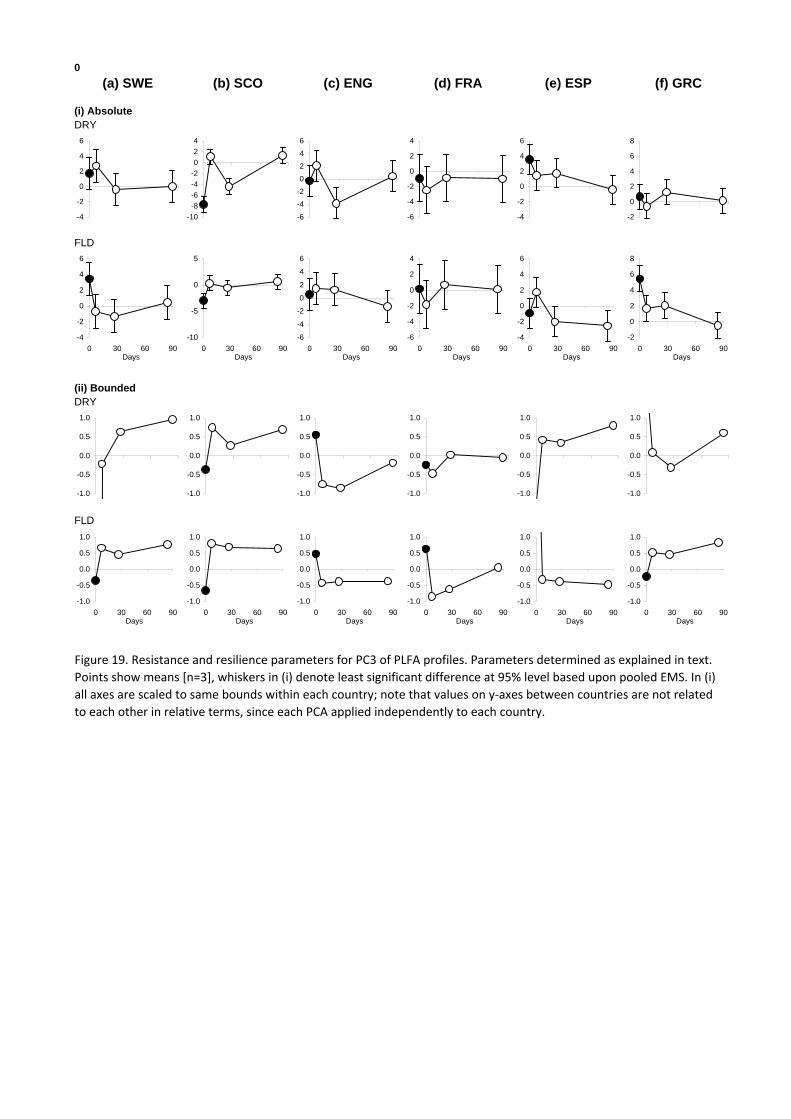
Establishing the degree of resistance and resilience for multivariate data such as PLFA profiles is less straightforward than for univariate properties. Principal component analysis is a technique which reduces the dimensionality of data in such a manner as to be appropriate to quantify resistance and resilience, since by definition if two PLFA profiles are congruent, the PCs will be concomitantly equal. Thus a community phenotype would be interpreted as completely resistant if the associated PCs were essentially the same between control and perturbed systems, and totally resilient if there were a convergence of PCs over time. When PCA was applied to data within each source country, there was generally highly significant temporal variation in all of the first four principal components, and some instances of significant perturbation effects and time x perturbation interactions (Figs. 13-16; combined ordinations are also presented in Supplementary Figures S1 – S6). Application of relative resistance and resilience indices is not appropriate due to the way the PCs are derived (there is an inherent data normalisation process which renders such proportionality nonsensical), but absolute- and bounded-indices (Figs. 17-20) should be applicable.

However, this is not the case for resistance where negative PCs are involved with the control (e.g. ESP for flooded soil in PC1; Figs. 13, 17), since the formula (Fig. 4(3)) does not take the absolute form for Co. As was the case for N mineralisation rates, there was poor correspondence in general between absolute and bounded resilience measures based upon PCs (Figs 17-20), due to the large temporal variation in the control soils (Figs. 13-16). Comparison of individual PCs provides a general basis for determining resistance and resilience, but a more revealing means of visualising the data to this end is to ordinate those PCs where significant perturbation effects were manifest. In this case, it is apparent that the phenotypes of the SWE and SCO soils were not resistant to drying, nor the GRC soil to flooding, and phenotypes of ESP soils showed an equitable but low resilience to flooding and drying (Fig. 21). By mapping the trajectories of such PCs over time thorough the ordinations, the temporal dynamics of the community phenotypes are apparent, and in all soils consistently converge to common zones in the PC ordinations at T84 (Fig. 21). This demonstrates that in all cases the community phenotypes in all soils were essentially resilient. In some cases, such as ENG and FRA soils, the trajectories between the control and perturbed soils were highly consistent (Figs. 21c, d), suggesting that there were inherent dynamics in the community structures in these soils which the drying and flooding perturbations temporarily modulated.

When the PLFA profiles for all soils were combined in a PCA, there were significant country and time effects for the first four PCs, such that ordination of the PC1-4 showed that the phenotypic profiles for each country were highly distinct (Fig 22). Ordination of PC2 and PC3, both of which showed significant effects of perturbation in ANOVA, showed that the relative sensitivity of the soils to the perturbations differed between countries (Fig. 23). Thus the GRC soils showed similar, but low resistance to both flooding and drying; the ESP soils showed low resistance to flooding, and the SWE soils were least resistant to drying (Fig. 23). All soils showed a high degree of resilience to both perturbation types, as shown by the general converge of points by T84 (Fig. 23), as also concluded from the PCA applied to individual countries (Fig. 21). This combined ordination also shows that the relative variability within countries differed markedly, with SCO, ENG and FRA soils being less variable compared to the GRC, ESP and SWE soils (Fig. 23).



21.65.2 18.211.0 6.9

44.111.9

GRC

MS p

0.616.37.8

ESP

MS p

13.6107.2 ***5.6

FRA

MS p

28.0 *77.6 ***9.9

ENG

MS p

1.286.0 ***6.1

p

SWE

Error 14.9

Time

MSSOURCE

3.433.4

Perturbation

PC

1

SCO

MS p

5.1

Pert x time 16.9

-10

-8

-6

-4

-2

0

2

4

6

0 10 20 30 40 50 60 70 80 90

ControlDryFlood

-10-8-6-4-202468

0 10 20 30 40 50 60 70 80 90-6

-4

-2

0

2

4

6

0 10 20 30 40 50 60 70 80 90

-6-4-202468

1012

0 10 20 30 40 50 60 70 80 90

Time (days)

-8-6-4-202468

0 10 20 30 40 50 60 70 80 90

Time (days)

-8-6-4-202468

10

0 10 20 30 40 50 60 70 80 90

Time (days)

Figure 13. First principal component (PC1) derived from PLFA profiles and associated ANOVA terms. PC analysis applied to each country independently (hence scales on y‐axes are not directly comparable). Points denote means [n=3] whiskers denote pooled standard errors. In ANOVA table, blank cell, P>0.05; * P<0.05; ** P<0.001; *** P<0.001.



PC

2

SCO

MS p

0.2

Pert x time 12.0

Perturbation

SOURCE

Error 5.6

Time

MS p

***

SWE

20.933.7 24.1 *

4.1

ENG

MS p

27.4 ***41.4 ***1.6

FRA

MS p

4.238.2 ***2.9

ESP

MS p

9.4 *60.0 ***4.6

GRC

MS p

1.239.6 ***5.3

6.3 2.8 4.94.2 2.1

-6

-4

-2

0

2

4

6

8

0 10 20 30 40 50 60 70 80 90

ControlDryFlood

-4-3-2-1012345

0 10 20 30 40 50 60 70 80 90-6

-4

-2

0

2

4

6

8

0 10 20 30 40 50 60 70 80 90

-6

-4

-2

0

2

4

6

0 10 20 30 40 50 60 70 80 90

Time (days)

-10

-8

-6

-4

-2

0

2

4

0 10 20 30 40 50 60 70 80 90

Time (days)

-8

-6

-4

-2

0

2

4

6

0 10 20 30 40 50 60 70 80 90

Time (days)

Figure 14. Second principal component (PC2) derived from PLFA profiles and associated ANOVA terms. PC analysis applied to each country independently (hence scales on y‐axes are not directly comparable). Points denote means [n=3] whiskers denote pooled standard errors. In ANOVA table, blank cell, P>0.05; * P<0.05; ** P<0.001; *** P<0.001.



2.07.1 2.81.5 4.5

1.36.0 *

GRC

MS p

16.1 **18.1 **5.4

ESP

MS p

19.5 **7.91.0

FRA

MS p

5.825.5 **8.3

ENG

MS p

2.56.1 *

15.1 ***

p

*

SWE

Error 3.4

Time

MSSOURCE3.2

11.3Perturbation

PC

2

SCO

MS p

18.4 ***

Pert x time 5.6

-4

-3

-2

-1

0

1

2

3

4

0 10 20 30 40 50 60 70 80 90

ControlDryFlood

-6-5-4-3-2-1012345

0 10 20 30 40 50 60 70 80 90-5-4-3-2-101234

0 10 20 30 40 50 60 70 80 90

-4-3-2-1012345

0 10 20 30 40 50 60 70 80 90

Time (days)

-5-4-3-2-1012345

0 10 20 30 40 50 60 70 80 90

Time (days)

-4-3-2-1012345

0 10 20 30 40 50 60 70 80 90

Time (days)

Figure 15.Third principal component (PC3) derived from PLFA profiles and associated ANOVA terms. PC analysis applied to each country independently (hence scales on y‐axes are not directly comparable). Points denote means [n=3] whiskers denote pooled standard errors. In ANOVA table, blank cell, P>0.05; * P<0.05; ** P<0.001; *** P<0.001.



2.22.4 1.71.7 2.6

4.92.1

GRC

MS p

5.221.0 ***3.0

ESP

MS p

5.014.7 **7.3 *

FRA

MS p

1.720.0 ***2.7

ENG

MS p

0.633.4 ***2.1

p

***

SWE

Error 1.4

Time

MSSOURCE0.2

24.4Perturbation

PC

2

SCO

MS p

3.0

Pert x time 2.3

-5-4-3-2-101234

0 10 20 30 40 50 60 70 80 90

ControlDryFlood

-4

-3

-2

-1

0

1

2

3

4

0 10 20 30 40 50 60 70 80 90-5-4-3-2-101234

0 10 20 30 40 50 60 70 80 90

-5-4-3-2-101234

0 10 20 30 40 50 60 70 80 90

Time (days)

-4-3-2-101234

0 10 20 30 40 50 60 70 80 90

Time (days)

-4

-3

-2

-1

0

1

2

3

0 10 20 30 40 50 60 70 80 90

Time (days)

Figure 16. Fourth principal component (PC4) derived from PLFA profiles and associated ANOVA terms. PC analysis applied to each country independently (hence scales on y‐axes are not directly comparable). Points denote means [n=3] whiskers denote pooled standard errors. In ANOVA table, blank cell, P>0.05; * P<0.05; ** P<0.001; *** P<0.001.

0

(i) AbsoluteDRY

FLD

(ii) BoundedDRY

FLD


-1.0

-0.5

0.0

0.5

1.0

-1.0

-0.5

0.0

0.5

1.0

-1.0

-0.5

0.0

0.5

1.0

-1.0

-0.5

0.0

0.5

1.0

-1.0

-0.5

0.0

0.5

1.0

-1.0

-0.5

0.0

0.5

1.0

-1.0

-0.5

0.0

0.5

1.0

0 30 60 90Days

-1.0

-0.5

0.0

0.5

1.0

0 30 60 90Days

-1.0

-0.5

0.0

0.5

1.0

0 30 60 90Days

-1.0

-0.5

0.0

0.5

1.0

0 30 60 90Days

-1.0

-0.5

0.0

0.5

1.0

0 30 60 90Days

-1.0

-0.5

0.0

0.5

1.0

0 30 60 90Days

-12-9-6-3036

-5

0

5

10

-10

-5

0

5

-6-4-202468

-10

-5

0

5

-12-8-4048

12

-12

-9

-6

-3

0

3

6

0 30 60 90Days

-5

0

5

10

0 30 60 90Days

-10

-5

0

5

0 30 60 90Days

-6-4-202468

0 30 60 90Days

-10

-5

0

5

0 30 60 90Days

-12

-8

-4

0

4

8

12

0 30 60 90Days

Figure 17. Resistance and resilience parameters for PC1 of PLFA profiles. Parameters determined as explained in text. Points show means [n=3], whiskers in (i) denote least significant difference at 95% level based upon pooled EMS. In (i) all axes are scaled to same bounds within each country; note that values on y‐axes between countries are not related to each other in relative terms, since each PCA applied independently to each country.

0

(i) AbsoluteDRY

FLD

(ii) BoundedDRY

FLD


-1.0

-0.5

0.0

0.5

1.0

-1.0

-0.5

0.0

0.5

1.0

-1.0

-0.5

0.0

0.5

1.0

-1.0

-0.5

0.0

0.5

1.0

-1.0

-0.5

0.0

0.5

1.0

-1.0

-0.5

0.0

0.5

1.0

-1.0

-0.5

0.0

0.5

1.0

0 30 60 90Days

-1.0

-0.5

0.0

0.5

1.0

0 30 60 90Days

-1.0

-0.5

0.0

0.5

1.0

0 30 60 90Days

-1.0

-0.5

0.0

0.5

1.0

0 30 60 90Days

-1.0

-0.5

0.0

0.5

1.0

0 30 60 90Days

-1.0

-0.5

0.0

0.5

1.0

0 30 60 90Days

-10-8-6-4-2024

-8-6-4-20246

-6-4-20246

-4

-2

0

2

4

6

-6

-4

-2

0

2

-6-4-20246

-10-8-6-4-2024

0 30 60 90Days

-8-6-4-20246

0 30 60 90Days

-6

-4

-2

0

2

4

6

0 30 60 90Days

-4

-2

0

2

4

6

0 30 60 90Days

-6

-4

-2

0

2

0 30 60 90Days

-6

-4

-2

0

2

4

6

0 30 60 90Days


0

(i) AbsoluteDRY

FLD

(ii) BoundedDRY

FLD


-1.0

-0.5

0.0

0.5

1.0

-1.0

-0.5

0.0

0.5

1.0

-1.0

-0.5

0.0

0.5

1.0

-1.0

-0.5

0.0

0.5

1.0

-1.0

-0.5

0.0

0.5

1.0

-1.0

-0.5

0.0

0.5

1.0

-1.0

-0.5

0.0

0.5

1.0

0 30 60 90Days

-1.0

-0.5

0.0

0.5

1.0

0 30 60 90Days

-1.0

-0.5

0.0

0.5

1.0

0 30 60 90Days

-1.0

-0.5

0.0

0.5

1.0

0 30 60 90Days

-1.0

-0.5

0.0

0.5

1.0

0 30 60 90Days

-1.0

-0.5

0.0

0.5

1.0

0 30 60 90Days

-4

-2

0

2

4

6

-10-8-6-4-2024

-6-4-20246

-6

-4

-2

0

2

4

-4

-2

0

2

4

6

-2

0

2

4

6

8

-4

-2

0

2

4

6

0 30 60 90Days

-10

-5

0

5

0 30 60 90Days

-6

-4

-2

0

2

4

6

0 30 60 90Days

-6

-4

-2

0

2

4

0 30 60 90Days

-4

-2

0

2

4

6

0 30 60 90Days

-2

0

2

4

6

8

0 30 60 90Days


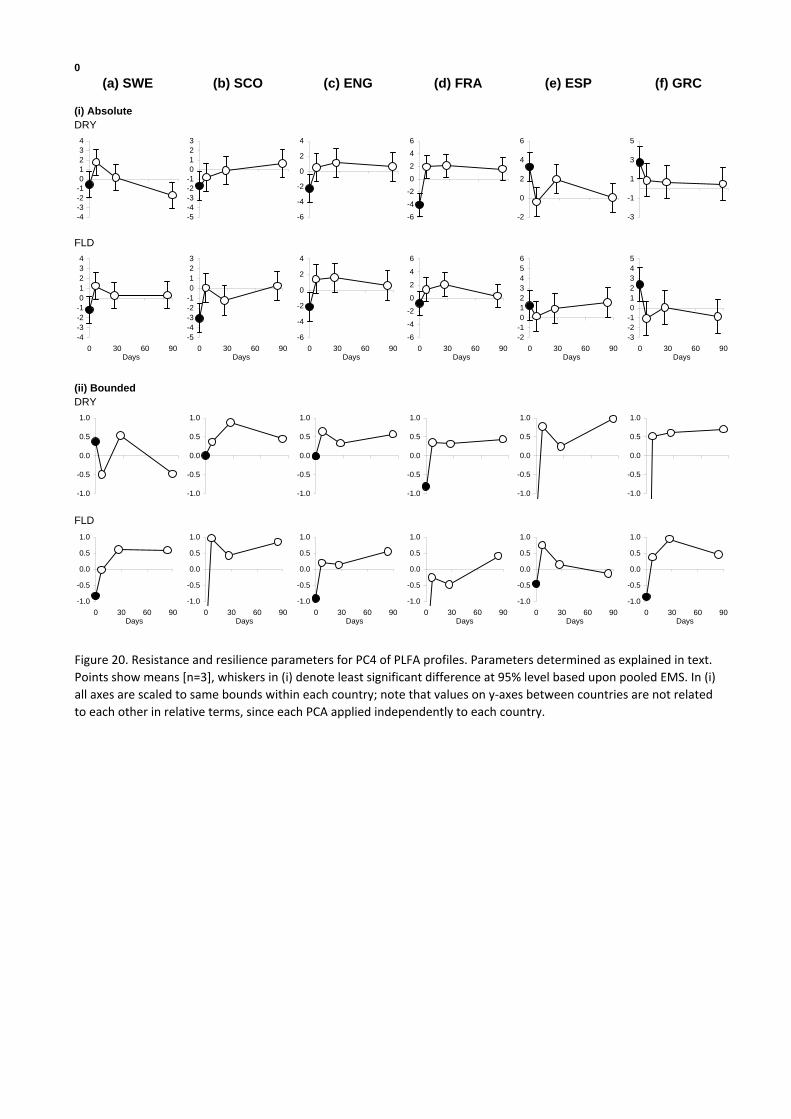
0

(i) AbsoluteDRY

FLD

(ii) BoundedDRY

FLD


-1.0

-0.5

0.0

0.5

1.0

-1.0

-0.5

0.0

0.5

1.0

-1.0

-0.5

0.0

0.5

1.0

-1.0

-0.5

0.0

0.5

1.0

-1.0

-0.5

0.0

0.5

1.0

-1.0

-0.5

0.0

0.5

1.0

-1.0

-0.5

0.0

0.5

1.0

0 30 60 90Days

-1.0

-0.5

0.0

0.5

1.0

0 30 60 90Days

-1.0

-0.5

0.0

0.5

1.0

0 30 60 90Days

-1.0

-0.5

0.0

0.5

1.0

0 30 60 90Days

-1.0

-0.5

0.0

0.5

1.0

0 30 60 90Days

-1.0

-0.5

0.0

0.5

1.0

0 30 60 90Days

-4-3-2-101234

-5-4-3-2-10123

-6

-4

-2

0

2

4

-6-4-20246

-2

0

2

4

6

-3

-1

1

3

5

-4-3-2-101234

0 30 60 90Days

-5-4-3-2-10123

0 30 60 90Days

-6

-4

-2

0

2

4

0 30 60 90Days

-6

-4

-2

0

2

4

6

0 30 60 90Days

-2-10123456

0 30 60 90Days

-3-2-1012345

0 30 60 90Days


(c) ENG

C00

C07

C27

C84

D00D07

D27

D84

F00F07F27

F84

-5

-4

-3

-2

-1

0

1

2

3

4

5

-4 -2 0 2 4 6 8PC1

PC

2

(d) FRA

C00

C07

C27

C84

D00

D07

D27

D84

F00F07F27

F84

-4

-3

-2

-1

0

1

2

3

4

5

-4 -2 0 2 4 6 8 10PC1

PC

2

(e) ESP

F84

F27

F07

F00 D84

D27

D07

D00

C84

C27

C07C00

-4

-3

-2

-1

0

1

2

3

4

-8 -6 -4 -2 0 2 4PC2

PC

3

F84

F27

F07

F00

D84

D27

D07

D00

C84

C27

C07

C00

-4

-3

-2

-1

0

1

2

3

-4 -2 0 2 4 6PC2

PC

4(a) SWE

F84

F27F07

F00

D84

D27

D07

D00

C84C27

C07

C00

-5

-4

-3

-2

-1

0

1

2

3

4

-8 -6 -4 -2 0 2 4 6PC1

PC

3

(b) SCO

F84

F27

F07

F00

D84D27

D07

D00

C84

C27

C07

C00

-3

-2

-1

0

1

2

3

4

-6 -4 -2 0 2 4PC2

PC

3

(f) GRC

Figure 21. Ordinations of principal components (PCs) derived from PLFA profiles of soils from each country separately. PCs were selected for plotting in the first instance on basis of whether they showed significant effect of perturbation, then which PC next showed greatest effect of time. Abbreviations: C = control; D = dry; F = flood; numbers denote days post application of perturbation (i.e. Tn in experimental notation). Broken arrows connect points relating to control soils to respective perturbed soils (i.e. resistance); solid arrows mark a notional trajectory through the ordination across time periods, drawn by visual estimation.

Source PCA1 PCA2 PCA3 PCA4

Source PC1 PC2 PC3 PC4Country *** *** *** ***Perturbation ** ** *Time *** *** *** ***Country*PerturbationCountry*Time * ***Perturbation*TimeCountry*Perturbation*Time

GRC

ESP

FRA

ENG

SCO

SWE

-3

-2

-1

0

1

2

3

4

-4 -3 -2 -1 0 1 2 3PC1 [24%]

PC2

[12%

]

GRC

ESP

FRAENG

SCOSWE

-2

-1

0

1

2

3

4

-6 -4 -2 0 2 4PC3 [11%]

PC

4 [9

%]

Figure 22.. Ordinations of principal components (PCs) derived from PLFA profiles based upon data combined from all countries and associated ANOVA terms. (a) PC1 vs PC2; (b) PC3 vs PC4. Points show means (n=36), bars show pooled standard errors; values in parentheses in axis labels denote percentage variation accounted for by the respective Eigenvalues.

(a)

(b)

F84

*

*

F00

D84

* *

D00C84

* *

C00

F84

*

*F00

D84

*

*

D00

C84

**

C00

F84

*

*

F00

D84

*

*

D00

C84

*

*C00

F84

**

F00

D84

*

*

D00

C84

*

*

C00F84

*

*

F00

D84 *

*

D00

C84

*

*C00

F84

*

*F00

D84*

*

D00

C84

**

C00

-6

-5

-4

-3

-2

-1

0

1

2

3

4

-8 -6 -4 -2 0 2 4

PC2

PC3

GRC

SWE

FRA

ENG

SCO

ESP

D00

Figure 23. Ordinations of second and third principal components (PC) derived from PLFA profiles based upon data combined from all countries. Points show means (n=4). Abbreviations: C = control; D = dry; F = flood; numbers denote days post application of perturbation (i.e. Tn in experimental notation). Only points relating to T0 and T84 are labelled for clarity; asterisks denote other points for T7 and T27. Broken arrows connect points relating to control soils to respective perturbed soils (i.e. resistance); solid arrows connect points relating to perturbed soils to their respective controls 84 days after perturbation (i.e. resilience). Ellipses are arbitrarily drawn around T0 and T84 boundaries to data for each country.


5.7 The importance of the control

There was a general trend across all parameters for significant temporal variation in the control soils, i.e. significant differences between data values at T84 compared to T0. This was particularly apparent from the phenotypic profiles, and in some instances there were apparently consistent trajectories in the way the PLFA profiles were changing over time. There was no evidence that the phenotypes at least had reached an equilibrium point after 84 days, only that the secondary effects of the perturbations upon the phenotypic structure had subsided by then. These dynamics could have arisen as a result of the soil disturbance during preparation of the microcosms, and are notable in that the mean respiration rates suggested microbial activity was declining over the entire period of 84 days. This suggests that, as was also apparent for the functional measurements, all soils were in a dynamic state during the incubation period in the experiment, but that the perturbations resulted in some deviations from these inherent dynamics, with a subsequent convergence. The process-based measurements were not sufficiently sensitive to detect such phenomena, but the PLFA profiling did. Part of the reason for this could be that the perturbations were relatively mild, and did not induce a large-scale response in the process-based parameters measured. PLFA profiling appears to be a sensitive measure of the status of the soil microbial community, which is also apparent in other studies (e.g. Defra Report SP0534). Previous resistance and resilience studies have tended to adopt more extreme perturbations such as heavy-metal or xenobiotic addition, or heat-shock (for review see Defra Report SP1605).

Temporal variation in the controls such as was encountered here affects the bounded resistance and resilience values and confounds the interpretation of such indices, since the ‘norm’ in this case is taken to be the value at T0, which in the case where controls are showing significant variation is arguably not appropriate. This can then result in the interpretation that that a system is not resilient when in actuality there is no difference between the property in perturbed or control systems at a common time after perturbation. In a sense, such systems would be arguably resilient – it depends upon the definition of the control, and what is deemed to be appropriate in this context. In general, and particularly in the natural state, soils (and ecosystems) are rarely in any state of true equilibrium and always in some form of dynamics, hence the static or ‘T0’ baseline view of resistance or resilience is inappropriate. We argue that the absolute and relative forms of resistance and resilience are the most appropriate measures. Relative indices generally show similar temporal patterns to absolute measures but can be misleading where data ranges are relatively large. For example, where the magnitude of properties are small, apparently very large relative (%) changes can be manifest but are a consequence of very small absolute changes (e.g. potential nitrification rates for GRC).

5.8 Overall resistance and resilience responses

A qualitative scoring of the overall responses of the soils to the perturbations shows that overall, soils were less resistant to drying than flooding (Table 1). This was particularly the case for the community phenotypic profiles, and notably so for the soils derived from the northern and southern extremes of the latitudinal gradient. In relative terms, there was some evidence that SCO in particular, but also ENG, soils showed least resistance across the piece (Table 1). There was also a distinct decrease in resistance to flooding in the phenotypic profiles down the latitudinal gradient, which circumstantially supports the hypothesis that communities in soils from more arid zones are more immediately affected by flooding. However, this assertion has to be qualified by the point that all the soils were in essence equally (and highly) resilient – a shown by the scarcity of noted effects in the resilience section of Table 1.


Table 1. Summary of resistance and resilience responses, in relative terms between countries, with respect to activity parameters and community phenotypic structure.

SWE SCO ENG FRA ESP GRC

RESISTANCE1

Drying

• Respiration

• Potential nitrification xx x x

• N mineralisation xx x xx

• Phenotypic structure xxx xxx x xx xx

Flooding

• Respiration

• Potential nitrification x

• N mineralisation

• Phenotypic structure x x xx xx xxx

RESILIENCE1

Drying

• Respiration

• Potential nitrification x x

• N mineralisation x

• Phenotypic structure

Flooding

• Respiration

• Potential nitrification x

• N mineralisation xx

• Phenotypic structure

• Blank cell = highly resistant/resilient: x = some lack of resistance/resilience; xx = lack of resistance/resilience; xxx = least resistance/resilience.


5.9 Performance of potential indicators of resistance and resilience

The potential indicators adopted here to determine resistance and resilience phenomena differed in the extent to which they satisfied the four primary criteria for effectiveness:

(i) Discrimination: the process-based assays discriminated between soils on the basis of their origin, and to a modest extent in relation to the perturbations. Phenotypic profiling was considerably more effective in this respect, strongly discriminating between soils with respect to origin, perturbation and time. There was also some coherence in such responses.

(ii) Sensitivity: In the scenarios tested here, sensitivity was very low for the process-based assays. However, phenotypic profiling was notably sensitive in that it allowed subtle effects of perturbation to be detected against a dynamic background.

(iii) Ubiquity: All of the processes measured gave signals from all of the soils and hence were ubiquitous. The failure to detect sufficient individuals in the worm assays suggest that such fauna are not ubiquitous and hence their application is on this basis questionable. PLFAs were ubiquitous in all the soils studied.

(iv) Interpretability: The key interpretation in the resistance and resilience assays relates to the behaviour of perturbed systems relative to a control. The difficulty in defining such an appropriate control notwithstanding, the basis of the resistance measure being the deviation from such controls and resilience the reversion to such comparators is in principal readily interpreted. Interpretation of multivariate data is a little less straightforward, but the ordination approaches here suggest that they too can be interpreted. There was circumstantial evidence in this study that the ecological interpretation of such resistance and resilience responses also appears robust.

6. Conclusions (i) Absolute indices of resistance and resilience are more readily interpreted since

they accommodate temporal variation in the control, and the extent of resistance and resilience can be readily visualised by plotting such differences between control and perturbed soils. It is also straightforward to determine the statistical significance of such differences since they are based upon primary data.

(ii) In general, the impact of the drying and flooding perturbations upon any of the properties was small, even immediately after removal of the perturbation. This was often particularly so relative to the general temporal variation which was apparent.

(iii) There was a range of responses between the soils from different sources, and with respect to the nature of the perturbation. There was tentative evidence that the phenotypes of more northern soils were more resistant flooding than those from more southern regions. All soils were resilient to the perturbations applied.

(iv) The prescription of the control in resistance and resilience assays is not straightforward if there are any dynamics in such controls which are large relative to the effect of the treatment. This could be attained by prolonged pre-incubation periods in non-disturbed systems, but this could arguably result in artificial circumstances.


(v) This study suggests that the resistance and resilience concept has some potential for application in pre-emptively determining the effects of, but perturbations need to be prescribed which have a more substantial impact upon response variables, or response variables which are less prone to variation in the absence of the putative stressors need to be considered. Extant work studying resistance and resilience phenomena have to date tended to adopt such circumstances, e.g. perturbation by adding heavy metals, heating the soil to unnaturally high temperatures, or compressive recovery.

(vi) For climate change scenarios in a UK context, water and temperature are acknowledged as being key variables and hence the perturbations need to involve these. In was not possible to include temperature-based perturbations within the scope of this study. However, the results here show that single instances of such perturbations had little impact on the soil phenotype or functioning. A logical development of the concept then is to study resistance and resilience phenomena during a series of repeated and sequential such perturbations, such as an intensive series of wet:dry and/or flood:drain events, possibly incorporating temperature treatments. Factorial combinations of such factors would be more incisive but the number of treatments soon escalates and sets a limit to the practicality of such approaches. High-throughput systems of measuring response variables would make such approaches more feasible, and there is clearly a rationale to develop such systems for phenotypic profiling of soil communities. A further metric which could be of pertinence is the number of such cycles which need to be applied before there is a substantive ‘state change’ in soil properties.

Acknowledgements We sincerely thank Anke Herrmann (Swedish University Agricultural Sciences), Guénola Peres (University of Rennes), Juan Puigdefábregas Tomás (CSIC Experimental Station for Arid Zones, Almería) and Sid Theocharopoulos (Soil Science Institute of Athens), and their colleagues, for their advice, interaction and assistance in procuring the soils used in this study. Woburn Park, Bedfordshire kindly gave permission to sample soil from their estate. We also thank Sue Welch and Jane Bingham of Cranfield University for technical support.

References Griffiths BS, Bonkowski M, Roy J, Ritz K (2001). Functional stability, substrate utilisation and biological indicators of soils following environmental impacts. Applied Soil Ecology 16, 49-61.

Griffiths BS, Ritz K, Bardgett RD, Cook R, Christensen S, Ekelund F, Sørensen S, Bååth E, Bloem J, de Ruiter PC, Dolfing J, Nicolardot B (2000). Ecosystem response of pasture soil communities to fumigation-induced microbial diversity reductions: an examination of the biodiversity-ecosystem function relationship. Oikos 90, 279-294.

Orwin KH, Wardle DA (2004). New indices for quantifying the resistance and resilience of soil biota to exogenous disturbances. Soil Biology and Biochemistry 36, 1907-1912.

Ritz K, Black HIJ, Campbell CD, Harris JA, Wood C (2009). Selecting ecological indicators for monitoring soils: a framework for balancing scientific opinion to assist policy development. Ecological Indicators 9, 1212-1221.

SWE

PERT TIME PxTPC1PC2PC3PC4

%3320 ***

7 ***9 *

F84F27

F07

F00

D84D27

D07

D00C84

C27

C07

C00

-4

-3

-2

-1

0

1

2

3

4

5

6

-8 -6 -4 -2 0 2 4

PC1

PC2

C00

C07

C27

C84

D00

D07

D27

D84

F00

F07

F27

F84

-4

-3

-2

-1

0

1

2

3

-3 -2 -1 0 1 2 3

PC3

PC4

8427

07

00

-3

-2

-1

0

1

2

3

4

-4 -2 0 2 4 6

PC1

PC2

F

D

C

-2.5

-2.0

-1.5

-1.0

-0.5

0.0

0.5

1.0

1.5

2.0

2.5

-2 -1 0 1 2

PC1

PC2

84

27

07

00

-3.0

-2.0

-1.0

0.0

1.0

2.0

3.0

-2 -1 0 1 2 3

PC3

PC4

F

DC

-0.6

-0.4

-0.2

0.0

0.2

0.4

0.6

-1.5 -1.0 -0.5 0.0 0.5 1.0 1.5

PC3

PC4

(a)

(b)

(c)

(d)

(e)

(f)

Figure S1. Ordinations of first four principal components (PCs) derived from PLFA profiles of SWE soils. Inset shows ANOVA terms.(a, b) perturbation:time means [n=3]; (c, d) means by time, across perturbations [n=9]; (e, f) means by perturbation, across time [n=12]. Abbreviations: C = control; D = dry; F = flood; numbers denote days post application of perturbation (i.e. Tn in experimental notation). Whiskers denote pooled standard errors, omitted from (a) and (b) for clarity. ANOVA terms: % = variation accounted for by the respective Eigenvalues; Blank cell, P>0.05; * P<0.05; ** P<0.001; *** P<0.001

SCO


%***33

15 ****

9***

***11 *

F84

F27

F07

F00

D84

D27D07

D00

C84

C27

C07

C00

-3

-2

-1

0

1

2

3

4

-10 -5 0 5 10

PC1

PC2

C00

C07

C27

C84

D00

D07

D27

D84

F00

F07

F27

F84

-4

-3

-2

-1

0

1

2

3

-6 -4 -2 0 2 4

PC3

PC4

84

27

07

00

-3

-2

-1

0

1

2

3

-5 0 5 10

PC1

PC2

FDC

-1.0

-0.8

-0.6

-0.4

-0.2

0.0

0.2

0.4

0.6

0.8

1.0

-2 -1 0 1 2

PC1

PC2

84

27

07

00

-4.0

-3.0

-2.0

-1.0

0.0

1.0

2.0

3.0

-2 -1 0 1 2

PC3

PC4

F

D

C

-1.0

-0.8

-0.6

-0.4

-0.2

0.0

0.2

0.4

0.6

0.8

1.0

-2.0 -1.0 0.0 1.0 2.0

PC3

PC4

(a)

(b)

(c)

(d)

(e)

(f)

Figure S2. Ordinations of first four principal components (PCs) derived from PLFA profiles of SCO soils. Inset shows ANOVA terms. (a, b) perturbation:time means [n=3]; (c, d) means by time, across perturbations [n=9]; (e, f) means by perturbation, across time [n=12]. Abbreviations: C = control; D = dry; F = flood; numbers denote days post application of perturbation (i.e. Tn in experimental notation). Whiskers denote pooled standard errors, omitted from (a) and (b) for clarity. ANOVA terms: % = variation accounted for by the respective Eigenvalues; Blank cell, P>0.05; * P<0.05; ** P<0.001; *** P<0.001

ENG

PERT TIME PxTPC1PC2PC3PC4 8 ***

14 **

%***27

15 ******

F84

F27F07 F00

D84

D27

D07D00

C84

C27C07

C00

-5

-4

-3

-2

-1

0

1

2

3

4

5

-4 -2 0 2 4 6 8

PC1

PC2

C00

C07

C27C84 D00

D07

D27

D84 F00

F07

F27

F84

-4

-3

-2

-1

0

1

2

3

-4 -2 0 2 4

PC3

PC4

84

2707

00

-3

-2

-1

0

1

2

3

4

5

-4 -2 0 2 4 6

PC1

PC2

F

D

C

-2.5

-2.0

-1.5

-1.0

-0.5

0.0

0.5

1.0

1.5

2.0

2.5

-2 -1 -1 0 1 1 2

PC1

PC2

84

27

07

00

-3.0-2.5-2.0-1.5-1.0-0.50.00.51.01.52.02.5

-4 -2 0 2 4

PC3

PC4

F

D C

-0.8

-0.6

-0.4

-0.2

0.0

0.2

0.4

0.6

0.8

-1.5 -1.0 -0.5 0.0 0.5 1.0 1.5

PC3

PC4

(a)

(b)

(c)

(d)

(e)

(f)

Figure S3. Ordinations of first four principal components (PCs) derived from PLFA profiles of ENG soils. Inset shows ANOVA terms. (a, b) perturbation:time means [n=3]; (c, d) means by time, across perturbations [n=9]; (e, f) means by perturbation, across time [n=12]. Abbreviations: C = control; D = dry; F = flood; numbers denote days post application of perturbation (i.e. Tn in experimental notation). Whiskers denote pooled standard errors, omitted from (a) and (b) for clarity. ANOVA terms: % = variation accounted for by the respective Eigenvalues; Blank cell, P>0.05; * P<0.05; ** P<0.001; *** P<0.001

FRA

PERT TIME PxTPC1PC2PC3PC4 *9 **

12

%***31

14 ******

F84

F27F07 F00

D84

D27

D07

D00

C84

C27

C07

C00

-4

-3

-2

-1

0

1

2

3

4

5

-5 0 5 10

PC1

PC2

C00C07

C27

C84

D00

D07

D27D84

F00

F07

F27

F84

-4

-3

-2

-1

0

1

2

3

-3 -2 -1 0 1 2 3

PC3

PC4

84

27

07 00

-3

-2

-1

0

1

2

3

4

-4 -2 0 2 4 6 8

PC1

PC2

F

D

C

-1.5

-1.0

-0.5

0.0

0.5

1.0

1.5

-3 -2 -1 0 1 2 3

PC1

PC2

84 27

07

00

-2.0

-1.5

-1.0

-0.5

0.0

0.5

1.0

1.5

2.0

2.5

3.0

-3 -2 -1 0 1 2 3

PC3

PC4

F

D

C

-1.0

-0.8

-0.6

-0.4

-0.2

0.0

0.2

0.4

0.6

0.8

1.0

-2.0 -1.0 0.0 1.0 2.0

PC3

PC4

(a)

(b)

(c)

(d)

(e)

(f)

Figure S4. Ordinations of first four principal components (PCs) derived from PLFA profiles of FRA soils. Inset shows ANOVA terms. (a, b) perturbation:time means [n=3]; (c, d) means by time, across perturbations [n=9]; (e, f) means by perturbation, across time [n=12]. Abbreviations: C = control; D = dry; F = flood; numbers denote days post application of perturbation (i.e. Tn in experimental notation). Whiskers denote pooled standard errors, omitted from (a) and (b) for clarity. ANOVA terms: % = variation accounted for by the respective Eigenvalues; Blank cell, P>0.05; * P<0.05; ** P<0.001; *** P<0.001

ESP

PERT TIME PxTPC1PC2PC3PC4 ***8

**11 **

%3316 ****

F84F27

F07

F00

D84D27D07

D00

C84

C27C07

C00

-8

-6

-4

-2

0

2

4

-6 -4 -2 0 2 4 6

PC1

PC2

C00

C07

C27

C84

D00

D07

D27D84F00

F07

F27

F84

-3

-2

-1

0

1

2

3

-4 -2 0 2 4

PC3

PC4

84

2707

00

-5

-4

-3

-2

-1

0

1

2

3

-4 -2 0 2 4

PC1

PC2

F

D C

-2.0

-1.5

-1.0

-0.5

0.0

0.5

1.0

1.5

-4 -2 0 2 4

PC1

PC2

84

27

07

00

-3.0

-2.5

-2.0

-1.5

-1.0

-0.5

0.0

0.5

1.0

1.5

2.0

-3 -2 -1 0 1 2

PC3

PC4

FD

C

-1.5

-1.0

-0.5

0.0

0.5

1.0

-2.0 -1.0 0.0 1.0 2.0 3.0

PC3

PC4

(a)

(b)

(c)

(d)

(e)

(f)

Figure S5. Ordinations of first four principal components (PCs) derived from PLFA profiles of ESP soils. Inset shows ANOVA terms. (a, b) perturbation:time means [n=3]; (c, d) means by time, across perturbations [n=9]; (e, f) means by perturbation, across time [n=12]. Abbreviations: C = control; D = dry; F = flood; numbers denote days post application of perturbation (i.e. Tn in experimental notation). Whiskers denote pooled standard errors, omitted from (a) and (b) for clarity. ANOVA terms: % = variation accounted for by the respective Eigenvalues; Blank cell, P>0.05; * P<0.05; ** P<0.001; *** P<0.001

GRC


*6

**7

%4216 ***

F84

F27

F07

F00

D84

D27 D07

D00

C84

C27

C07

C00

-6

-5

-4

-3

-2

-1

0

1

2

3

-6 -4 -2 0 2 4 6

PC1

PC2

C00

C07

C27C84

D00D07

D27

D84

F00

F07

F27

F84

-3

-2

-2

-1

-1

0

1

1

2

2

-4 -2 0 2 4

PC3

PC4

84

27 07

00

-4

-3

-2

-1

0

1

2

3

4

-6 -4 -2 0 2 4

PC1

PC2

FD

C

-1.0

-0.5

0.0

0.5

1.0

1.5

-2 -1 0 1 2

PC1

PC2

84

27

0700

-1.5

-1.0

-0.5

0.0

0.5

1.0

1.5

2.0

-2 -1 -1 0 1 1 2

PC3

PC4

F

D

C

-1.0

-0.5

0.0

0.5

1.0

1.5

-2.0 -1.0 0.0 1.0 2.0

PC3

PC4

(a)

(b)

(c)

(d)

(e)

(f)

Figure S6. Ordinations of first four principal components (PCs) derived from PLFA profiles of GRC soils. Inset shows ANOVA terms. (a, b) perturbation:time means [n=3]; (c, d) means by time, across perturbations [n=9]; (e, f) means by perturbation, across time [n=12]. Abbreviations: C = control; D = dry; F = flood; numbers denote days post application of perturbation (i.e. Tn in experimental notation). Whiskers denote pooled standard errors, omitted from (a) and (b) for clarity. ANOVA terms: % = variation accounted for by the respective Eigenvalues; Blank cell, P>0.05; * P<0.05; ** P<0.001; *** P<0.001

Country Perturbation Time log(PNR+1) a b c d e f g h i j k l m n o p q r s t u v w x y z # $ENG Control T00 0.455 x x x xENG Control T07 0.580 x x x x xENG Control T27 0.884 x x x x x x xENG Control T84 0.961 x x x x x x xENG Dry T00 0.253 x x xENG Dry T07 0.536 x x x xENG Dry T27 0.958 x x x x x x xENG Dry T84 1.044 x x x x xENG Flood T00 0.668 x x x x x x xENG Flood T07 0.589 x x x x xENG Flood T27 1.208 x xENG Flood T84 0.941 x x x x x x xESP Control T00 0.822 x x x x x xESP Control T07 0.879 x x x x x x xESP Control T27 1.445 x xESP Control T84 0.924 x x x x x xESP Dry T00 0.965 x x x x x x xESP Dry T07 0.913 x x x x x x xESP Dry T27 1.579 xESP Dry T84 1.249 x x xESP Flood T00 0.838 x x x x x x xESP Flood T07 0.907 x x x x x xESP Flood T27 1.360 x xESP Flood T84 1.130 x x xFRA Control T00 0.469 x x x xFRA Control T07 0.704 x x x x x x xFRA Control T27 1.070 x x x xFRA Control T84 1.068 x x x xFRA Dry T00 0.652 x x x x x x xFRA Dry T07 0.660 x x x x x xFRA Dry T27 1.035 x x x x x xFRA Dry T84 1.045 x x x x xFRA Flood T00 0.215 x xFRA Flood T07 0.643 x x x x x x xFRA Flood T27 1.049 x x x x xFRA Flood T84 1.039 x x x x x xGRC Control T00 0.215 x xGRC Control T07 0.083 xGRC Control T27 0.554 x x x xGRC Control T84 0.478 x x xGRC Dry T00 0.134 x xGRC Dry T07 0.326 x x xGRC Dry T27 0.563 x x x xGRC Dry T84 0.458 x x x xGRC Flood T00 0.172 x xGRC Flood T07 0.336 x x xGRC Flood T27 0.492 x x x xGRC Flood T84 0.437 x x xSCO Control T00 2.313 x x xSCO Control T07 2.210 xSCO Control T27 2.488 x xSCO Control T84 2.276 x xSCO Dry T00 1.852 xSCO Dry T07 2.293 x x xSCO Dry T27 2.381 x x xSCO Dry T84 2.249 xSCO Flood T00 2.305 x x xSCO Flood T07 2.195 xSCO Flood T27 2.510 xSCO Flood T84 2.251 xSWE Control T00 0.640 x x x x x x xSWE Control T07 0.813 x x x x x xSWE Control T27 1.145 x x xSWE Control T84 0.967 x x x x x x xSWE Dry T00 0.652 x x x x x x xSWE Dry T07 0.624 x x x x x x xSWE Dry T27 0.797 x x x x x x xSWE Dry T84 0.964 x x x x x x xSWE Flood T00 0.603 x x x x x xSWE Flood T07 0.764 x x x x x x xSWE Flood T27 0.990 x x x x x xSWE Flood T84 0.946 x x x x x x x

Table S1. Homogeneous groups for mean potential nitrifictaion rate based upon Fisher test at 95% level of significance. Means belong to homogeneous groups where ‘x’ symbol shares common letter in columns.

Country Perturbation Time Nmin rate a b c d e f g h i j k l m n o p q r s tENG Control T00 0.40 x x x x x x x x xENG Control T07 0.40 x x x x x x x x x xENG Control T27 0.39 x x x x x x x x x xENG Control T84 0.57 x x x x x x xENG Dry T00 0.60 x x x x xENG Dry T07 0.28 x x x x x x x x x xENG Dry T27 0.42 x x x x x x x x xENG Dry T84 0.54 x x x x x x x xENG Flood T00 0.37 x x x x x x x x xENG Flood T07 0.16 x x xENG Flood T27 0.54 x x x x x x x x xENG Flood T84 0.65 x x xESP Control T00 0.50 x x x x x x x x x xESP Control T07 0.37 x x x x x x x x x xESP Control T27 0.34 x x x x x x x x x xESP Control T84 0.35 x x x x x x x x x x xESP Dry T00 0.46 x x x x x x x x xESP Dry T07 0.40 x x x x x x x x xESP Dry T27 0.25 x x x x x x x xESP Dry T84 0.33 x x x x x x x x x xESP Flood T00 0.50 x x x x x x x x x xESP Flood T07 0.39 x x x x x x x x x xESP Flood T27 0.41 x x x x x x x x xESP Flood T84 0.27 x x x x x x x x xFRA Control T00 0.67 xFRA Control T07 0.47 x x x x x x x x x xFRA Control T27 0.61 x x x xFRA Control T84 0.23 x x x x x x x xFRA Dry T00 0.46 x x x x x x x x xFRA Dry T07 0.64 x x x xFRA Dry T27 0.58 x x x x x xFRA Dry T84 0.47 x x x x x x x x x xFRA Flood T00 0.68 xFRA Flood T07 0.66 x xFRA Flood T27 0.58 x x x x x xFRA Flood T84 0.25 x x x x x x x xGRC Control T00 0.24 x x x x x x x xGRC Control T07 0.12 xGRC Control T27 0.21 x x x x x xGRC Control T84 0.14 xGRC Dry T00 0.22 x x x x x x xGRC Dry T07 0.12 xGRC Dry T27 0.39 x x x x x x x x x xGRC Dry T84 0.17 x x xGRC Flood T00 0.28 x x x x x x x x x xGRC Flood T07 0.12 xGRC Flood T27 0.26 x x x x x x x xGRC Flood T84 0.13 xSCO Control T00 0.29 x x x x x x x x x xSCO Control T07 0.22 x x x x x x x xSCO Control T27 0.23 x x x x x x x xSCO Control T84 0.22 x x x x x x xSCO Dry T00 0.61 x x x xSCO Dry T07 0.24 x x x x x x x xSCO Dry T27 0.19 x x x x xSCO Dry T84 0.16 x xSCO Flood T00 0.30 x x x x x x x x x xSCO Flood T07 0.24 x x x x x x x xSCO Flood T27 0.18 x x x xSCO Flood T84 0.21 x x x x x xSWE Control T00 0.38 x x x x x x x x x xSWE Control T07 0.22 x x x x x x x xSWE Control T27 0.23 x x x x x x x xSWE Control T84 0.24 x x x x x x x xSWE Dry T00 0.52 x x x x x x x x x xSWE Dry T07 0.35 x x x x x x x x x x xSWE Dry T27 0.26 x x x x x x x xSWE Dry T84 0.26 x x x x x x x xSWE Flood T00 0.33 x x x x x x x x x xSWE Flood T07 0.28 x x x x x x x x x xSWE Flood T27 0.25 x x x x x x x xSWE Flood T84 0.50 x x x x x x x x x x

Table S2. Homogeneous groups for mean N mineralisation rate based upon Fisher test at 95% level of significance. Means belong to homogeneous groups where ‘x’ symbol shares common letter in columns.

Documents

Department for Environment, Food and Rural Affairs ...sciencesearch.defra.gov.uk/Document.aspx?Document=DefraSP057… · Department for Environment, Food and Rural Affairs Research