Embed Size (px)
Citation preview

Density Forecast inFunctional Space
Joe J. QianDepartment of Economics
Rice University
Page 1

Contents
(1.) Motivations.
(2.) FAR(1) Model of Time-Varying Densities
(3.) Estimation and Forecast
(4.) A Simulation
(5.) An Application in Risk-Neutral Density Forecast
(6.) Conclusions
Page 2

Part 1
Motivations
Page 3

Pseudo-Panel Data Set
(Xit), i = 1, · · · , N, t = 1, · · · , T
• (Example I) Xit can be income, energy consumption, etc., forhousehold i at time t.
• (Example II) Xit = Ct(Ki), where Ct(Ki) are option priceswith strike prices Ki at time t.
Page 4

Time-Varying Distributions
(pt), t = 1, · · · , T
• (Example I) The pdf of (X1t, X2t, · · · , XN,t)
• (Example II) Risk-neutral pdf implicit in option pricesCt(Ki), i = 1, 2, · · · , N at time t.
Page 5
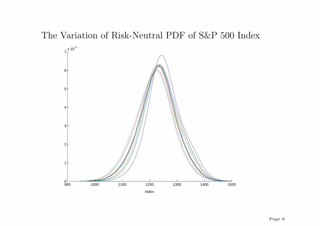
The Variation of Risk-Neutral PDF of S&P 500 Index
900 1000 1100 1200 1300 1400 15000
1
2
3
4
5
6
7x 10
−3
Index
Page 6
Part 2
FAR(1) Model of Time-Varying Densities
Page 7

Functional AR(1) Model
Time-varying densities: {pt(x)}, t ∈ Z, x ∈ [a, b]
pt − Ep0 = A(pt−1 − Ep0) + εt, t ∈ Z. (1)
Page 8

AR(1) in Moments
Lemma: If (f, λ) is an eigenfunction-eigenvalue pair of A∗,
Etf(X)− Ef(X) = λ(Et−1f(X)− Ef(X)) + ηt.
Page 9

AR(1) and ARCH(1)
If (fj) is Legendre series,
EtXj − EXj = λj(Et−1X
j − EXj) + ηt, j = 1, 2
Page 10

ARCH-M
If A∗ is some appropriate integral operator,
EtX = αEt−1X + βEt−1X2 + ηt.
Page 11
Part 3
Estimation and Forecast
Page 12

Estimation of Density
pNt = pt + ∆Nt, t = 1, · · · , T,
E‖∆Nt‖2 = O(N−r)
• (Example I) Estimate pdf of (X1t, X2t, · · · , XN,t)
pNt(x) =1
Nh
N∑
i=1
K(x−Xit
h)
• (Example II) Estimate risk-neutral density implicit in optionprices Ct(Ki), i = 1, 2, · · · , N at time t.
pNt(x) = erτ ∂C2(x)∂x2
Page 13
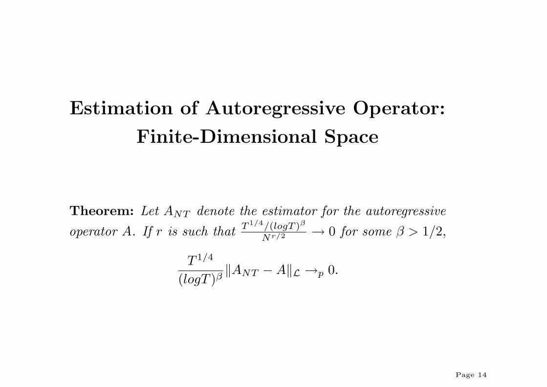
Estimation of Autoregressive Operator:
Finite-Dimensional Space
Theorem: Let ANT denote the estimator for the autoregressiveoperator A. If r is such that T 1/4/(logT )β
Nr/2 → 0 for some β > 1/2,
T 1/4
(logT )β‖ANT −A‖L →p 0.
Page 14

Estimation of Autoregressive Operator:
Infinite-Dimensional Space
Theorem: Under some technical conditions, if A isHilbert-Schmidt,
‖ANT −A‖L →p 0.
Page 15
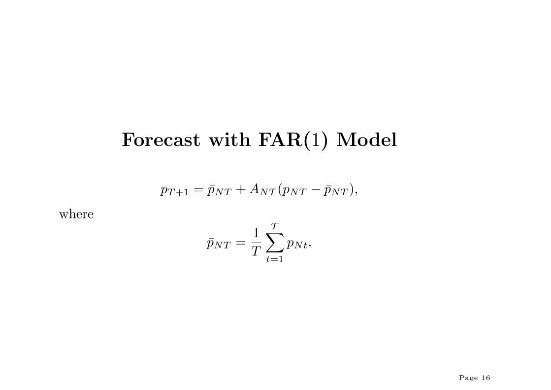
Forecast with FAR(1) Model
pT+1 = pNT + ANT (pNT − pNT ),
where
pNT =1T
T∑t=1
pNt.
Page 16

Part 4
A Simulation
Page 17

Data Generating Process
Let θt = (µt, σ2t , βt)′ be a VAR(1) process.
Xit ∼ Nt + Ut,
Nt = Normal(µt, σ2t )
Ut = Uniform(βt − σt, βt + σt)
Page 18

Simulation Result
Table 1: Monte Carlo Simulation Result
MSE in Moments PredictionSRISE Mean Variance Skewness Kurtosis
pN,T+1 (FAR(1)) 0.0441 0.0658 0.112 0.103 0.167
pNT (Average) 0.0476 0.0753 0.136 0.102 0.163
pNT (Last) 0.0546 0.0703 0.118 0.140 0.235
Parametric n/a 0.066 0.139 n/a n/aNote: SRISE denotes Square Root of Integrated Square Error,
SRISE(p) =qR
(p(x)− p(x))2dx, where p is the reference density
function.
Page 19
Part 5
Empirical Application in ForecastingRisk-Neutral Density
Page 20
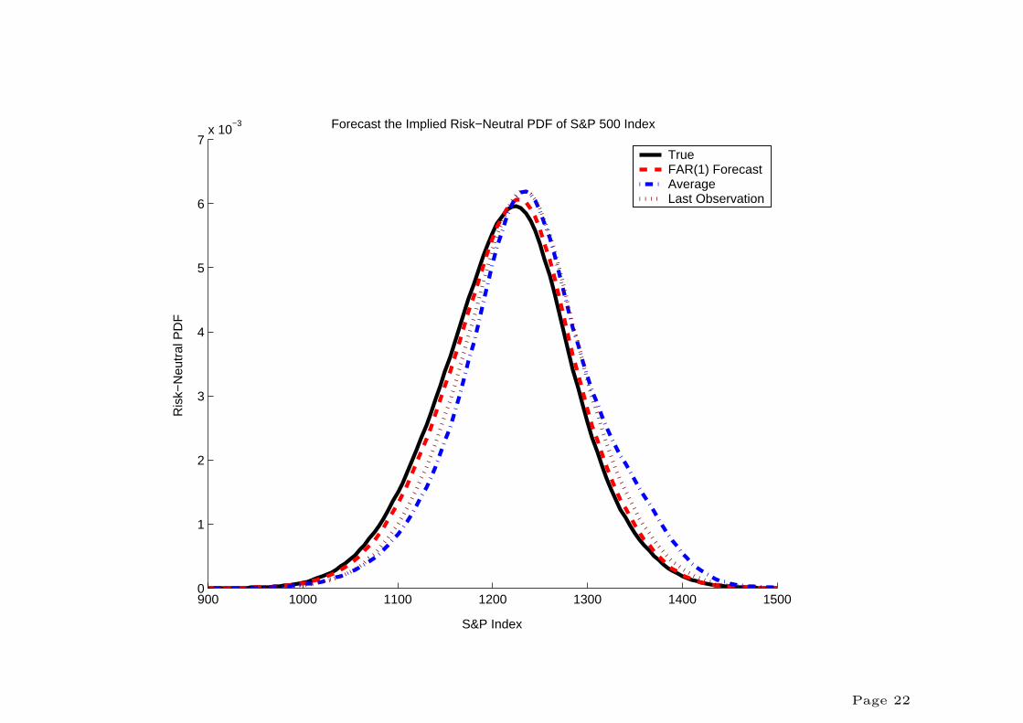
Data Description
We have daily European call prices on the S&P 500 Index that
mature on December 15 2004. We choose the prices from August16th 2004 to November 30th 2004, estimate risk-neutral density foreach day, and forecast the risk-neutral density on the next businessday, December 1st 2004.
Page 21
900 1000 1100 1200 1300 1400 15000
1
2
3
4
5
6
7x 10
−3
S&P Index
Ris
k−N
eutr
al P
DF
Forecast the Implied Risk−Neutral PDF of S&P 500 Index
TrueFAR(1) ForecastAverageLast Observation
Page 22

True FAR Average Last
Mean 1214.78 1219.37 1237.77 1229.50
Volatility 71.17 70.61 72.93 69.44
Skewness -0.104 -0.121 -0.0254 -0.0747
Kurtosis 3.182 3.203 3.293 3.242
SRISE 0 0.0032 0.0132 0.0092
Table 2: Numerical Evaluation
Page 23

Conclusions
• Introduction of functional AR method for modelling timevarying densities. We show that it embeds models such asscalar AR, ARCH, ARCH-M, etc.
• The consistency of the estimator of autoregressive operatorunder conditions on the convergence of functional estimators.
• The application of FAR(1) model to Risk-Neutral PDFforecast. This provides yet another tool to risk managementand option pricing.
Page 24