Embed Size (px)
Citation preview
DENSITY-BASED CLUSTERING OF HIGH-DIMENSIONAL DNA
FINGERPRINTS FOR LIBRARY-DEPENDENT MICROBIAL
SOURCE TRACKING
A Thesis
presented to
the Faculty of California Polytechnic State University,
San Luis Obispo
In Partial Fulfillment
of the Requirements for the Degree
Master of Science in Computer Science
by
Eric Johnson
December 2015

c© 2015
Eric Johnson
ALL RIGHTS RESERVED
ii

COMMITTEE MEMBERSHIP
TITLE: Density-Based Clustering of High-Dimensional DNA Fingerprints forLibrary-Dependent Microbial SourceTracking
AUTHOR: Eric Johnson
DATE SUBMITTED: December 2015
COMMITTEE CHAIR: Alexander Dekhtyar, Ph.D.Professor of Computer Science
COMMITTEE MEMBER: Zoe Wood, Ph.D.Professor of Computer Science
COMMITTEE MEMBER: Christopher Kitts, Ph.D.Professor and Chair of Biology
iii
ABSTRACT
Density-Based Clustering of High-Dimensional DNA Fingerprints for
Library-Dependent Microbial Source Tracking
Eric Johnson
As part of an ongoing multidisciplinary effort at California Polytechnic State Uni-
versity, biologists and computer scientists have developed a new Library-dependent
Microbial Source Tracking method for identifying the host animals causing fecal con-
tamination in local water sources. The Cal Poly Library of Pyroprints (CPLOP) is
a database which stores E. coli representations of fecal samples from known hosts
acquired from a novel method developed by the biologists called Pyroprinting. The
research group considers E. coli samples whose Pyroprints match above a certain
threshold to be part of the same bacterial strain. If an environmental sample from
an unknown host matches one of the strains in CPLOP, then it is likely that the host
of the unknown sample is the same species as one of the hosts that the strain was
previously found in. Clustering is a computer science technique for finding groups
of related data (i.e. strains) in a data set. In this thesis, we evaluate the use of
density-based clustering for identifying strains in CPLOP. Density-based clustering
finds clusters of points which have a minimum number of other points within a given
radius. We contribute a clustering algorithm based on the original DBSCAN algo-
rithm which removes points from the search space after they have been seen once. We
also present a new method for comparing pyroprints which is algebraically related to
the current method.The method has mathematical properties which make it possible
to use Pyroprints in a spatial index we designed especially for Pyroprints, which can
be utilized by the DBSCAN algorithm to speed up clustering.
iv

TABLE OF CONTENTS
Page
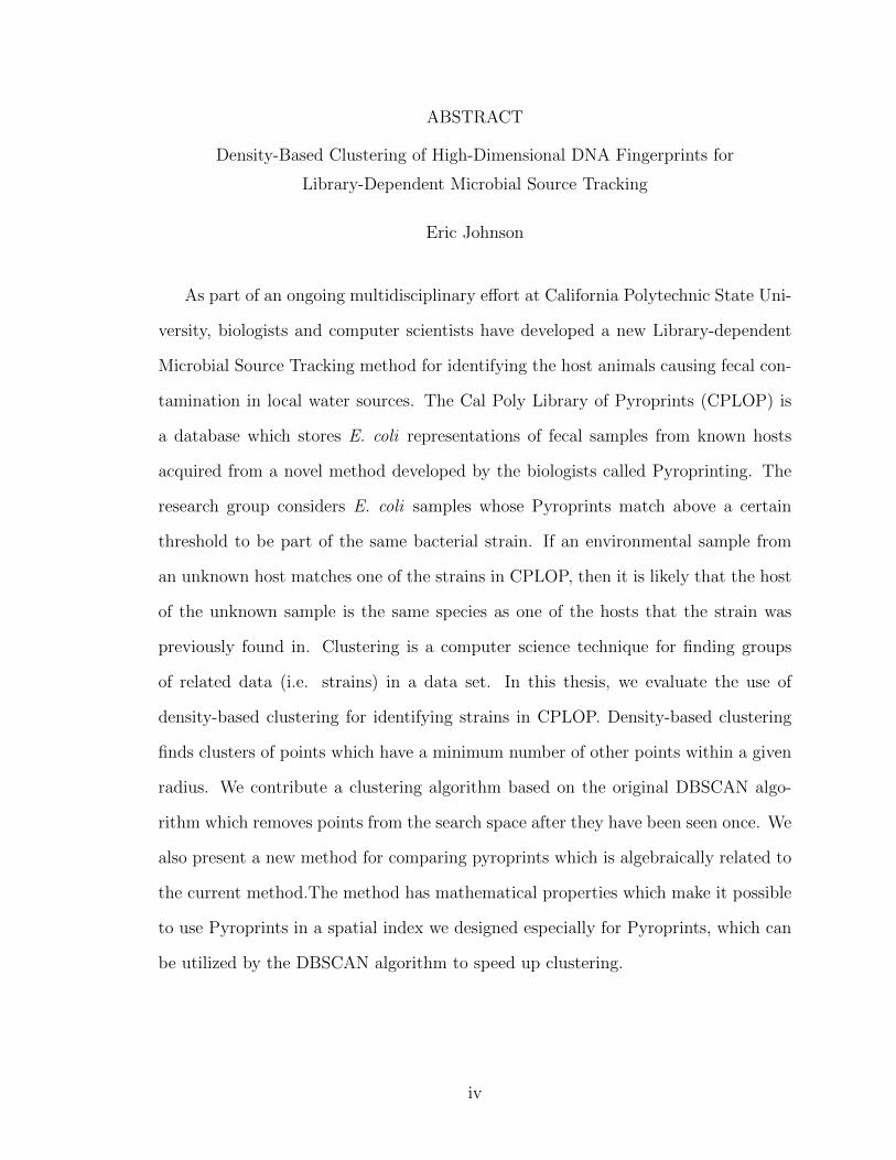
LIST OF TABLES . . . . . . . . . . . . . . . . . . . . . . . . . . . . . . . . . viii
LIST OF FIGURES . . . . . . . . . . . . . . . . . . . . . . . . . . . . . . . . ix
CHAPTER
1 INTRODUCTION . . . . . . . . . . . . . . . . . . . . . . . . . . . . . . . 1
2 BACKGROUND . . . . . . . . . . . . . . . . . . . . . . . . . . . . . . . . 7
2.1 Microbial Source Tracking (MST) . . . . . . . . . . . . . . . . . . . . 7
2.1.1 Library-Dependent MST . . . . . . . . . . . . . . . . . . . . . 8
2.1.2 Representations . . . . . . . . . . . . . . . . . . . . . . . . . . 10
2.2 Pyroprinting . . . . . . . . . . . . . . . . . . . . . . . . . . . . . . . . 10
2.2.1 Pyrosequencing . . . . . . . . . . . . . . . . . . . . . . . . . . 11
2.2.2 Gene Repetition and ITS regions . . . . . . . . . . . . . . . . 12
2.2.3 Pyroprints . . . . . . . . . . . . . . . . . . . . . . . . . . . . . 14
2.2.4 Pearson Correlation . . . . . . . . . . . . . . . . . . . . . . . . 15
2.2.5 Statistical Analysis and Strain Definition . . . . . . . . . . . . 15
2.3 CPLOP: Cal Poly Library of Pyroprints . . . . . . . . . . . . . . . . 17
2.4 Clustering . . . . . . . . . . . . . . . . . . . . . . . . . . . . . . . . . 19
2.4.1 OHClust!: Ontological Hierarchical Clustering . . . . . . . . . 19
2.4.2 DBSCAN: Density-Based Spatial Clustering of Applications withNoise . . . . . . . . . . . . . . . . . . . . . . . . . . . . . . . . 20
2.5 Spatial Indexes . . . . . . . . . . . . . . . . . . . . . . . . . . . . . . 22
2.5.1 Space Partitioning . . . . . . . . . . . . . . . . . . . . . . . . 25
2.5.2 Bounding Volume Hierarchy . . . . . . . . . . . . . . . . . . . 27
2.5.3 Hybrid Spatial Index . . . . . . . . . . . . . . . . . . . . . . . 28
3 DESIGN . . . . . . . . . . . . . . . . . . . . . . . . . . . . . . . . . . . . . 29
3.1 Motivation And Goals . . . . . . . . . . . . . . . . . . . . . . . . . . 29
3.2 Overview . . . . . . . . . . . . . . . . . . . . . . . . . . . . . . . . . . 30
3.2.1 Speeding Up MST . . . . . . . . . . . . . . . . . . . . . . . . 30
3.2.2 Allowing Strain Analysis . . . . . . . . . . . . . . . . . . . . . 30
v

3.2.3 Scaling With a Growing Database . . . . . . . . . . . . . . . . 31
3.3 Isolate Comparison . . . . . . . . . . . . . . . . . . . . . . . . . . . . 33
3.3.1 Euclidean Distance of Pyroprint Z-Scores . . . . . . . . . . . . 33
3.3.2 Considering Multiple DNA Regions . . . . . . . . . . . . . . . 36
3.4 Spatial Index . . . . . . . . . . . . . . . . . . . . . . . . . . . . . . . 37
3.4.1 Optimizations for use with DBSCAN . . . . . . . . . . . . . . 38
3.4.2 Data Characteristics . . . . . . . . . . . . . . . . . . . . . . . 39
3.4.3 Construction . . . . . . . . . . . . . . . . . . . . . . . . . . . 40
3.4.4 Storage . . . . . . . . . . . . . . . . . . . . . . . . . . . . . . 42
3.4.5 Algorithms . . . . . . . . . . . . . . . . . . . . . . . . . . . . 44
3.5 Clustering . . . . . . . . . . . . . . . . . . . . . . . . . . . . . . . . . 47
3.5.1 Modified DSBCAN Algorithm . . . . . . . . . . . . . . . . . . 49
4 IMPLEMENTATION . . . . . . . . . . . . . . . . . . . . . . . . . . . . . . 54
4.1 Language and Libraries . . . . . . . . . . . . . . . . . . . . . . . . . . 54
4.2 Overview . . . . . . . . . . . . . . . . . . . . . . . . . . . . . . . . . . 55
4.3 Data Types . . . . . . . . . . . . . . . . . . . . . . . . . . . . . . . . 56
4.4 Indexes . . . . . . . . . . . . . . . . . . . . . . . . . . . . . . . . . . . 58
4.5 DBSCAN . . . . . . . . . . . . . . . . . . . . . . . . . . . . . . . . . 60
4.6 Evaluation . . . . . . . . . . . . . . . . . . . . . . . . . . . . . . . . . 61
5 EVALUATION . . . . . . . . . . . . . . . . . . . . . . . . . . . . . . . . . 63
5.1 Evaluation Plan . . . . . . . . . . . . . . . . . . . . . . . . . . . . . . 63
5.1.1 Performance Evaluation . . . . . . . . . . . . . . . . . . . . . 63
5.1.2 Strain Correctness . . . . . . . . . . . . . . . . . . . . . . . . 64
5.1.3 Similarity to Current Method . . . . . . . . . . . . . . . . . . 67
5.2 Isolate Sets . . . . . . . . . . . . . . . . . . . . . . . . . . . . . . . . 69
5.3 Clustering Parameters . . . . . . . . . . . . . . . . . . . . . . . . . . 70
5.3.1 DBSCAN . . . . . . . . . . . . . . . . . . . . . . . . . . . . . 70
5.3.2 Agglomerative Clustering and OHClust! . . . . . . . . . . . . 71
5.4 Clusters Statistics . . . . . . . . . . . . . . . . . . . . . . . . . . . . . 71
5.5 Evaluation Results . . . . . . . . . . . . . . . . . . . . . . . . . . . . 73
5.5.1 Performance Evaluation . . . . . . . . . . . . . . . . . . . . . 74
5.5.2 Strain Correctness . . . . . . . . . . . . . . . . . . . . . . . . 76
vi

5.5.3 Similarity to Current Method . . . . . . . . . . . . . . . . . . 79
6 CONCLUSION . . . . . . . . . . . . . . . . . . . . . . . . . . . . . . . . . 83
6.1 Future Work . . . . . . . . . . . . . . . . . . . . . . . . . . . . . . . . 84
6.1.1 E. coli Strains . . . . . . . . . . . . . . . . . . . . . . . . . . . 84
6.1.2 Performance . . . . . . . . . . . . . . . . . . . . . . . . . . . . 85
6.1.3 Additional Analysis Opportunities . . . . . . . . . . . . . . . . 86
6.1.4 Correctness . . . . . . . . . . . . . . . . . . . . . . . . . . . . 87
6.1.5 Applications . . . . . . . . . . . . . . . . . . . . . . . . . . . . 88
BIBLIOGRAPHY . . . . . . . . . . . . . . . . . . . . . . . . . . . . . . . . . 89
vii
LIST OF TABLES
Table Page
3.1 Converted Thresholds . . . . . . . . . . . . . . . . . . . . . . . . . 35
3.2 Number of dimensions with a standard deviation in various rangesfor each ITS region. . . . . . . . . . . . . . . . . . . . . . . . . . . . 39
5.1 Various statistics about the clusters produced by each method . . . 72
5.2 Distribution of cluster sizes for each clustering method . . . . . . . 73
5.3 Running times of clustering methods for increasing dataset sizes inseconds. . . . . . . . . . . . . . . . . . . . . . . . . . . . . . . . . . 74
5.4 RAM usage of clustering methods for increasing dataset sizes in MB 75
5.5 Time in seconds to perform a neighbor query for all isolates withdifferent spatial storage types . . . . . . . . . . . . . . . . . . . . . 76
5.6 Correctness of clustering methods with respect to the α and β thresh-olds. . . . . . . . . . . . . . . . . . . . . . . . . . . . . . . . . . . . 77
5.7 Results from 2-Sample Kolmogorov-Smirnov Goodness of Fit againstdistribution of Pearson Correlations between replicated isolates . . 79
5.8 Similarity Metrics of clusters compared to those of Agglomerativeclustering . . . . . . . . . . . . . . . . . . . . . . . . . . . . . . . . 80
5.9 Results from 2-Sample Kolmogorov-Smirnov Goodness of Fit againstAgglomerative clustering . . . . . . . . . . . . . . . . . . . . . . . . 81
viii
LIST OF FIGURES
Figure Page
2.1 A sample pyrogram, the result of pyrosequencing. . . . . . . . . . . 11
2.2 The rRNA operons in E. coli are present in seven copies, each ofwhich has two Internal Transcribed Spacer (ITS) regions . . . . . . 13
2.3 Beta distribution for pyroprints from the same isolate for ITS region16-23 . . . . . . . . . . . . . . . . . . . . . . . . . . . . . . . . . . . 17
2.4 Example density-based cluster with MinPts=3 . . . . . . . . . . . . 21
2.5 Pseudocode for the DBSCAN algorithm. . . . . . . . . . . . . . . . 22
2.6 Pseudocode for the DBSCAN algorithm . . . . . . . . . . . . . . . 23
2.7 Binary Search Tree example . . . . . . . . . . . . . . . . . . . . . . 24
2.8 Example KD-Tree . . . . . . . . . . . . . . . . . . . . . . . . . . . 26
2.9 Example R-Tree . . . . . . . . . . . . . . . . . . . . . . . . . . . . 26
3.1 Pseudocode for the algorithm that constructs our spatial index. . . 45
3.2 Pseudocode for our range query algorithm . . . . . . . . . . . . . . 46
3.3 Pseudocode for our range query algorithm . . . . . . . . . . . . . . 47
3.4 Pseudocode for our range query algorithm . . . . . . . . . . . . . . 47
3.5 Pseudocode for our modified DBSCAN algorithm . . . . . . . . . . 52
3.6 Pseudocode for our modified DBSCAN algorithm . . . . . . . . . . 53
4.1 SQL query for extracting isolates from CPLOP. . . . . . . . . . . . 57
4.2 SQL query for finding the distribution of pairwise Pearson correla-tions from replicates in CPLOP. . . . . . . . . . . . . . . . . . . . . 62
5.1 The ontology definition used by OHClust! to generate clusters forthe evaluation . . . . . . . . . . . . . . . . . . . . . . . . . . . . . . 72
ix

CHAPTER 1
INTRODUCTION
Clean sources of water are important for preventing the spread of diseases, and for
maintaining the environment. One of the undesirable contaminants often found in
bodies of water is feces[17]. The bacteria found along with fecal matter can make
animals, including humans, sick. Environmental and Resource agencies are interested
in finding the sources of fecal contamination. If the origin of contamination can be
ascertained, then actions can be taken to remove or reduce the amount of fecal matter
in the water.
The study of identifying and discriminating fecal bacteria in the environment
is called Microbial Source Tracking (MST). MST techniques usually look for fecal
indicator bacteria (FIB) in environmental samples[19]. These FIB are bacteria found
in the digestive tracts of animals, called hosts, that sometimes leave the animals along
with fecal matter. Investigators can look at the quantity of FIB in an environmental
sample to estimate the amount of fecal contamination in the sampled environment[17].
Additionally, they can examine individual bacteria found in the sample and try to
determine what host species they came from[17]. Generally, investigators are not
interested in finding the exact individual host from which the bacterium came, but
instead are satisfied with knowing the species of the host.
At the intersection of the fields of Computer Science and Biology lies a method
of MST called library-dependent MST[19]. Library-dependent MST works off the
assumption that there exist subgroups of an FIB species, called strains, which are
only found in certain host species[17]. The method starts with the collection of
a large number of bacteria samples from fecal matter from a known host species.
Representations of these bacteria are stored in a database along with the information
1

about their provenance. Once the database is established, MST is performed by
comparing environmental samples from unknown hosts to the samples stored in the
database with the hope of finding a match. If matching bacteria are found, then
researchers can look up the host species of the matching sample in the database and
use that as evidence that the unknown sample came from the same host species.
Simply determining that two bacteria are of the same species is not necessarily
enough to determine that two samples of FIB came from the same host species. In
fact, a common FIB species used for MST, Escherichia coli (E. coli), is found in the
guts and fecal matter of many host animals[17]. Instead, researchers must determine
that the bacteria both came from the same subgroup of the species. The idea is
that the more closely related two individuals are, the more recently they came from
a common ancestor and thus the more likely they came from the same host species.
Any meaningful subdivision of bacteria beyond species like this is called a strain.
MST research groups formally define their notion of a strain by picking a metric of
similarity and a threshold at which they are confident that bacteria are as closely
related as their metric can determine; maximizing the probability that the bacteria
came from a common ancestor and thus the same host.
Many methods can be used to measure the similarity between two bacteria cul-
tures. The methods can be classified by whether they look at the phenotypes of the
bacteria or the genotypes. Phenotypic comparison looks at appearance or behavior of
the bacteria, for example their reaction to a certain chemical[17]. Genotypic compari-
son on the other hand looks at the actual DNA of the bacteria. Comparing genotypes
can be more expensive but is generally more discerning[19], as similar appearance or
behavior can be produced by different sequences of DNA.
As part of an ongoing multidisciplinary effort at California Polytechnic State Uni-
versity, biologists and computer scientists have developed a new library-dependent
2
MST method. The Cal Poly Library of Pyroprints (CPLOP) is a database developed
by the computer scientists to support a novel, cost-effective genotype representa-
tion method for bacteria comparison developed by the biologists called Pyroprinting.
CPLOP uses E. coli as it’s FIB, storing representations acquired by running this
Pyroprinting method on E. coli samples. To increase discrimination ability of the
method, each E. coli sample’s DNA is pyroprinted in two separate locations. The
research group considers E. coli samples which match in both locations with a sim-
ilarity above a certain threshold to be part of the same strain. If that strain has
only been seen in one host species then they have good evidence that environmental
samples matching bacteria in that strain are also from the same host species.[20]
The number of samples stored in the database for library-dependent MST in-
fluences the confidence in matches found with unknown samples. As the size of
the database increases, so does the time to search for matches. In the case of the
naive search method, an unknown sample must be compared to every sample in the
database. At the time of this writing, MST in CPLOP[13] still relied on this method.
If the notion of strains were to be stored in the database, then unknown samples
could be compared to groups of bacteria in the database instead of every individual
bacterium, speeding up the search. Storing strains in the database would also facili-
tate other kinds of research. Longitudinal studies, such as that performed by Emily
Neal[15], look at strains observed in an individual over time and look for changes or
patterns. Transference studies, such as that performed by Josh Dillard[7], look at
samples from different hosts for strains found in both hosts.
The desire for a method of identifying strains from the set of bacteria in the
database is clear. Clustering is a computer science technique for finding groups of
related data (i.e. strains) in a data set. There are different definitions of which data
is part of the same group, or cluster. This is similar to the variation in definition of
a strain in biology. Thus the choice of clustering method must match the biologist’s
3

idea of what constitutes a strain for their research.
In previous work for CPLOP, Aldrin Montana developed a method of clustering
called OHClust![14]. OHClust! is based on agglomerative hierarchical clustering and
utilizes information about the provenance of samples to allow efficient addition to
the known clusters through incremental updates. Unfortunately, OHClust! cannot
run on the CPLOP servers which have meager memory resources. In addition, in his
evaluation of the clusters identified by OHClust!, Montana was unable to determine
if the clusters matched the biologist’s notion of strains.[14]
The work presented in this thesis provides an alternate solution for identifying
strains which hopes to address the limitations of OHClust!. It evaluates density-based
clustering for the use in identifying E. coli strains from pyroprints. Density-based
clustering, as defined by DBSCAN[9] finds clusters where points have a minimum
number of other points within a given radius. The DBSCAN algorithm can find
clusters like this very efficiently, especially if the points are stored in a spatial index.
The contributions of this thesis are the following:
• A modified DBSCAN algorithm: This is the first time density-based clus-
ters have been tried with CPLOP. The original algorithm for finding density-
based clusters was DBSCAN. Many researchers have provided modified versions
of this algorithm suited for different purposes. This thesis modifies DBSCAN,
allowing for the removal of points from the search space after they have been
seen once. This modification results in a 2x speedup for our use case.
• A faster method for comparing pyroprints: Prior to this work, pyroprints
in CPLOP were compared with Pearson Correlation. Pearson correlation ig-
nores certain differences in the pyroprints which are due to inconsistencies in
the physical pyroprinting process. This thesis presents a new method for com-
paring pyroprints which is algebraically related to the old method, allowing
4
reuse of previous statistical analysis. In addition we precomputed some inter-
mediate values which speeds up comparisons with both the old method and
the new method. The new method was chosen such that it has mathematical
properties which make it possible to treat the pyroprints as if they were points
in multidimensional space.
• A spatial index that works with E. coli pyroprints: The DBSCAN al-
gorithm can take advantage of storing data in a special way to increase the
efficiency. If the points being clustered are points in space, then they can be
stored based off their position in space. This is called a spatial index. Spatial in-
dexes can be searched quickly for points near another point. This thesis presents
a spatial index tailored for the needs of the data in CPLOP. It supports dense,
high-dimensional data, by partitioning the search space with multidimensional
planes as well as storing bounding volumes for groups of data. It also supports
multiple regions for each data point with separate search radii.
• Better evaluation metrics of clusters for CPLOP: Finally, this thesis
contributes an evaluation of the clusters generated by this work as well as those
generated by OHClust!. This evaluation was more thorough than that provided
in Montana’s Thesis, and is able to quantify how well the clusters match the
Biologist’s notion of a strain. Unlike Montana’s evaluation, this evaluation
goes beyond measuring the similarity of clusters to those produced by another
clustering method.
The rest of this document is organized as follows. Chapter 2 provides detailed
background information about both the biology and computer science sides of the
problem context. Chapter 3 provides a detailed explanation of the design for the
solution presented along with this thesis, as well as rational for design decisions.
Chapter 4 provides relevant details about the solution implementation along with
5

the benefits or limitations of particular implementation choices. Chapter 5 outlines
the evaluation performed on the solution followed by the results of the tests and
analysis of those results. Finally, Chapter 6 concludes the paper and suggests areas
of improvement as well as ideas for other related avenues of research.
6

CHAPTER 2
BACKGROUND
This chapter provides context for the work presented with this thesis. Faculty from
the Biology department at California Polytechnic University (Cal Poly) in conjunc-
tion with Computer Scientists from Cal Poly have developed a new method of mi-
crobial source tracking. This method is library-dependent and utilizes a novel DNA
fingerprinting technique, called pyroprinting, developed at Cal Poly. The Biology de-
partment has a desire to identify bacterial strains in the library. The work presented
in this thesis fulfils that desire using clustering and spatial indexes. It is an alternate
solution to OHClust! created by Aldrin Montana[14].
2.1 Microbial Source Tracking (MST)
The pyroprinting technique was developed by Biologists at Cal Poly as a tool for
microbial source tracking (MST)[5]. MST is the study of identifying and discriminat-
ing bacteria in the environment. Usually, the bacteria in question are found in fecal
matter contaminating environmental resources such as bodies of water. MST tech-
niques usually look for fecal indicator bacteria (FIB) in environmental samples[19].
These FIB are bacterial species found in the digestive tracts of animals, called hosts,
that sometimes leave the animals along with fecal matter. Investigators can look at
the quantity of an FIB in an environmental sample to estimate the amount of fecal
contamination in the sampled environment[17]. Additionally, they can examine indi-
vidual bacteria found in the sample and try to determine what host species they came
from[17]. Generally, investigators are not interested in finding the exact individual
host from which the bacterium came from, but instead are satisfied with knowing the
7

species of the host. The waste from a single animal has a minimal impact on the
cleanliness of a body of water, while the waste from a whole group can have a large
impact.
2.1.1 Library-Dependent MST
The MST method developed by the Biologists at Cal Poly is classified as library-
dependent. Library-dependent MST lies at the intersection of the fields of Computer
Science and Biology. Library-dependent MST works off of the assumption that there
exist subgroups of an FIB species which are only found in certain host species[17].
The method starts with the collection of a large number of bacterial samples from
fecal matter of a known host species. Representations of these bacteria are stored
in a database along with the information about the samples provenance. Once the
database is established, MST is performed by comparing environmental samples from
unknown hosts to the samples stored in the database with the hope of finding a match.
If matching bacteria are found, then researchers can look up the host species of the
matching sample in the database and use that as evidence that the unknown sample
came from the same host species.
Library-dependent MST is typically organized as follows:
1. Collection: The first step is to collect microbial samples from fecal matter of
known origin. When collected, the host species of the fecal matter is recorded.
Additional information such as location where the fecal matter was found, and
date of the collection can be recorded if desired for additional analysis oppor-
tunities, but is not necessary for MST.
2. Isolation: A sample of fecal matter contains many individual bacteria. Library-
dependent MST uses individual bacterial cultures, or isolates, taken from these
samples. The process used by the biologists at Cal Poly to isolate E. coli
8
bacteria from the rest of the sample is described by Black et al.[5]. Multiple
isolates can be taken from the same sample. The isolates can be cultured and
frozen to replicate them for future experiments.
3. Digital Representation: After a single bacterium is isolated, researchers must
then obtain a digital representation of the isolate. These representations are
meant to be compared to each other in order to determine whether the isolates
they match can be distinguished from each other. There are many different
methods of obtaining these representations, and different types of represen-
tations that can result. Some examples are discussed in Section 2.1.2. The
pyroprinting technique developed at Cal Poly is one of these methods.
4. Addition to Library: Next, the DNA representation is added to the library
along with metadata about the isolate it represents. The metadata includes
the information recorded in step 1, especially the host species of the origin
sample. Additionally, information about the isolate, and parameters for the
representation can be stored for bookeeping purposes, and to ensure consistency.
5. Forensics: Once the library has grown sufficiently large (through multiple
iterations of the previous steps), the system can then be used for MST. An en-
vironmental sample is collected and processed according to steps 2-3 to produce
an E. coli isolate from an unknown host. The resulting representation of this
isolate is then compared against the representations of isolates in the library.
If it matches any isolates in the library, then researchers look up the metadata
of those isolates. It is up to the researches to come to a conclusion based on
the amount and variety of host information from matching isolates about what
host the environmental isolate likely came from.
9
2.1.2 Representations
Many methods can be used to measure the similarity between two bacteria. The
methods can be classified by whether they look at the phenotypes of the bacteria
or the genotypes. Comparing genotypes can be more expensive but is generally
more discerning[19], as similar appearance or behavior can be produced by different
sequences of DNA.
Phenotypic comparison looks at appearance/behavior of the bacteria. The idea
is that bacteria from the same host species have adapted their behavior for survival
in the particular environment encountered in the guts of the host species. Exam-
ple representations that capture these traits include, results from biochemical tests,
antibiotic resistance, and profiles of the proteins found on the outer membrane.[17]
Genotypic comparison on the other hand looks at the DNA sequence from the
bacteria. The idea is that the more closely the DNA of two individuals are, the more
recently they came from a common ancestor and thus the more likely they came from
the same host species. A naive representation would simply be the full DNA sequence
of the bacteria, however that would be expensive and impractical for both creation and
comparison of the representations. Instead, researchers take shortcuts like measuring
the size differences of DNA fragments related to a specific location (ribotyping), or
by sequencing only a small part of the DNA which is highly variable[19].
2.2 Pyroprinting
Pyroprinting is a novel method of bacterial representation developed at Cal Poly
by Michael W. Black, Jennifer VanderKelen, Anya Goodman, and Christopher L.
Kitts[5]. They created the technique to address the problem they saw of researchers
needing to choose between representations with good discrimination, and represen-
10

Figure 2.1: A sample pyrogram, the result of pyrosequencing. Values represent
the heights of peaks.
tations that were cheap/convenient to generate. Pyroprinting bridges the gap by
providing both features. They are currently using pyroprints for MST with E. coli.
2.2.1 Pyrosequencing
Cal Poly’s pyroprinting method is based off of the DNA sequencing method called
pyrosequencing. The method is popular because it is a cheap and efficient way to
sequence short DNA fragments.
Pyrosequencing works on short sequences of DNA called regions. The region of
DNA is determined by primers. A primer is a short fragment of DNA that binds to
a specific complimentary DNA sequence, opening up the double helix. Two primers
are needed, one to bind to the start of the region of interest and the other binding
to the end. Once the primers are in place, DNA is copied from only that region.
Pyrosequencing needs lots of copies of this region, so the region is repeatedly copied,
or amplified, using the Polymerase Chain Reaction (PCR)[5].
Pyrosequencing is performed by a pyrosequencer machine which takes an amplified
region of DNA and outputs a vector of data called a pyrogram as shown in Figure
2.1. This pyrogram can be used to reconstruct the sequence of nucleotides present in
the sequenced region.
11
Pyrosequencing works by building a copy of the DNA strand and measuring the
light given off by the resulting chemical reactions. Along with the DNA, the re-
searchers provide a primer. The primer binds to a specific part of the DNA, and the
DNA is copied sequentially starting from that location. The DNA is copied in stages
called dispensations. One type of nucleotide is added per dispensation. Machines can
usually run for around 100 dispensations. The machine records the amount of light
emitted which is proportional to the number of nucleotides added to the copy during
that dispensation. The resulting pyrogram is a graph of light emitted at each stage
of the dispensation.
2.2.2 Gene Repetition and ITS regions
In order to be able to use pyrosequencing results to compare pyrograms between
different isolates, the same region needs to be sequenced every time. This means the
same primers need to be used every time. Primers are specific to specific DNA which
means the sequenced region has to start with the same DNA sequence for every
bacteria in the species. These regions exist in the DNA, and are called conserved
regions. They are regions of DNA that are important genes which if mutated would
result in the death of the cell, and thus those mutations would not be passed on to
progeny. However, if only the conserved region is sequenced, all isolates would get
the same representation. Ideally, the sequenced region would be highly variable, one
which has little or no effect on the life of the bacteria. Regions between genes, or
Internal Transcribed Spacers (ITS), as shown in Figure 2.2 fit this criteria. The way
to get a representation from a region that is highly variable but is in the same place
for different isolates is start pyrosequencing at the end of a conserved gene, then
continue sequencing into the ITS region. The research group is interested in 2 ITS
regions: ITS1 and ITS2. In the remainder of the thesis, each ITS region is referred
to as the genes which surround it: ITS1 = 16-23 and ITS2 = 23-5.
12
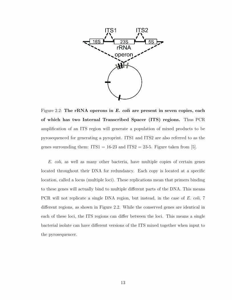
Figure 2.2: The rRNA operons in E. coli are present in seven copies, each
of which has two Internal Transcribed Spacer (ITS) regions. Thus PCR
amplification of an ITS region will generate a population of mixed products to be
pyrosequenced for generating a pyroprint. ITS1 and ITS2 are also referred to as the
genes surrounding them: ITS1 = 16-23 and ITS2 = 23-5. Figure taken from [5].
E. coli, as well as many other bacteria, have multiple copies of certain genes
located throughout their DNA for redundancy. Each copy is located at a specific
location, called a locus (multiple loci). These replications mean that primers binding
to these genes will actually bind to multiple different parts of the DNA. This means
PCR will not replicate a single DNA region, but instead, in the case of E. coli, 7
different regions, as shown in Figure 2.2. While the conserved genes are identical in
each of these loci, the ITS regions can differ between the loci. This means a single
bacterial isolate can have different versions of the ITS mixed together when input to
the pyrosequencer.
13

2.2.3 Pyroprints
Pyroprints are what the biologists at Cal Poly call the result of pyrosequencing a
region of DNA with multiple loci. Because pyroprinting uses pryosequencing, the
output of pyroprinting is a pyrogram. These pyrograms have different properties
from pyrograms of true DNA sequences, and so are named pyroprints to differentiate
the two. Specifically, pyroprints cannot be used to determine the DNA sequence
of the region. This is because a pyroprint represents multiple variations (loci) of
a given region. There is no way of knowing with this method whether all loci are
the same, each is different, or something in between. Therefore, when examining a
dispensation of a pyroprint, it is impossible to determine the distribution of added
nucleotides among the loci. This property is why the biologists needed novel software
and algorithms to perform MST with pyroprints.
In order to digitize a pyroprint, the biologists decided to take the maximum peak
height from each dispensation. Other options were peak width and peak area. For-
mally, the result is a vector ~p of length D
~p = (p1, p2, . . . , pD−1, pD)
where D is the number of dispensations of the pyroprint and each pi is a positive real
number.
To increase discrimination ability of the method, each E. coli sample’s DNA is
pyroprinted in two separate locations, 16S-23S and 23S-5S. In order to be considered
indistinguishable, the representations of two isolates must match for both regions.
Formally, an isolate’s representation is:
I = (~p16−23, ~p23−5)
14
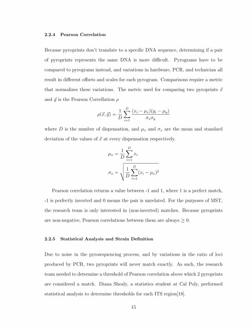
2.2.4 Pearson Correlation
Because pyroprints don’t translate to a specific DNA sequence, determining if a pair
of pyroprints represents the same DNA is more difficult. Pyrograms have to be
compared to pyrograms instead, and variations in hardware, PCR, and technician all
result in different offsets and scales for each pyrogram. Comparisons require a metric
that normalizes these variations. The metric used for comparing two pyroprints ~x
and ~y is the Pearson Correllation ρ
ρ(~x, ~y) =1
D
D∑i=1
(xi − µx)(yi − µy)σxσy
where D is the number of dispensation, and µx and σx are the mean and standard
deviation of the values of ~x at every dispensation respectively.
µx =1
D
D∑i=1
xi
σx =
√√√√ 1
D
D∑i=1
(xi − µx)2
Pearson correlation returns a value between -1 and 1, where 1 is a perfect match,
-1 is perfectly inverted and 0 means the pair is unrelated. For the purposes of MST,
the research team is only interested in (non-inverted) matches. Because pyroprints
are non-negative, Pearson correlations between them are always ≥ 0.
2.2.5 Statistical Analysis and Strain Definition
Due to noise in the pyrosequencing process, and by variations in the ratio of loci
produced by PCR, two pyroprints will never match exactly. As such, the research
team needed to determine a threshold of Pearson correlation above which 2 pyroprints
are considered a match. Diana Shealy, a statistics student at Cal Poly, performed
statistical analysis to determine thresholds for each ITS region[18].
15
In order to get a set of pyroprints which are supposed to match, the biologists made
repetitive pyroprints of multiple isolates. They then took pairwise Pearson correlation
values of pairs of pyroprints from the same isolate. This set of Pearson correlations
was a sample of the distribution of Pearson correlations between pyroprints with the
same DNA in the ITS regions.
First, Shealy analyzed the effect of dispensation count on the Pearson correlation
values. Pyrogram values get more noisy in later dispensations, because in the py-
rosequencer machines, chemicals and proteins are not completely removed between
each dispensation. So on one hand, using more dispensations decreased the Pearson
value for isolates that are supposed to match. On the other hand, using less dispen-
sations decreased the ability of Pearson correlation to capture differences between
pyroprints from truly different sources. The research group decided to only use 95
and 93 dispensations of the pyrogram for the ITS regions 16-23 and 23-5 respectively.
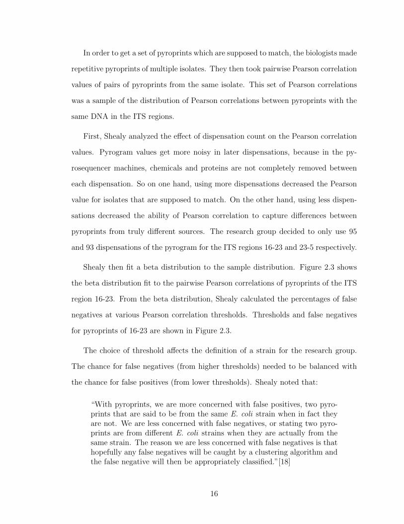
Shealy then fit a beta distribution to the sample distribution. Figure 2.3 shows
the beta distribution fit to the pairwise Pearson correlations of pyroprints of the ITS
region 16-23. From the beta distribution, Shealy calculated the percentages of false
negatives at various Pearson correlation thresholds. Thresholds and false negatives
for pyroprints of 16-23 are shown in Figure 2.3.
The choice of threshold affects the definition of a strain for the research group.
The chance for false negatives (from higher thresholds) needed to be balanced with
the chance for false positives (from lower thresholds). Shealy noted that:
“With pyroprints, we are more concerned with false positives, two pyro-prints that are said to be from the same E. coli strain when in fact theyare not. We are less concerned with false negatives, or stating two pyro-prints are from different E. coli strains when they are actually from thesame strain. The reason we are less concerned with false negatives is thathopefully any false negatives will be caught by a clustering algorithm andthe false negative will then be appropriately classified.”[18]
16
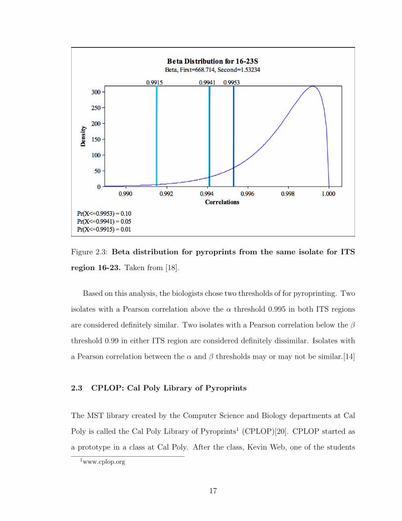
Figure 2.3: Beta distribution for pyroprints from the same isolate for ITS
region 16-23. Taken from [18].
Based on this analysis, the biologists chose two thresholds of for pyroprinting. Two
isolates with a Pearson correlation above the α threshold 0.995 in both ITS regions
are considered definitely similar. Two isolates with a Pearson correlation below the β
threshold 0.99 in either ITS region are considered definitely dissimilar. Isolates with
a Pearson correlation between the α and β thresholds may or may not be similar.[14]
2.3 CPLOP: Cal Poly Library of Pyroprints
The MST library created by the Computer Science and Biology departments at Cal
Poly is called the Cal Poly Library of Pyroprints1 (CPLOP)[20]. CPLOP started as
a prototype in a class at Cal Poly. After the class, Kevin Web, one of the students
1www.cplop.org
17

from the class, completed CPLOP as his senior project. Later, Jan Soliman made
extensive upgrades to CPLOP dubbed CPLOP 2.0[20].
CPLOP stores pyroprints and the provenance metadata associated with them in
a relational database. The work of this thesis integrates with CPLOP. It takes its
input from the pyroprint database, and stores its output there.
The primary use for CPLOP is microbial source tracking. MST is discussed in
depth in Section 2.1. Other uses for CPLOP include facilitating longitudinal and
transference studies. Longitudinal studies, such as that performed by Emily Neal[15],
look at strains observed in an individual over time and look for changes or patterns.
Transference studies, such as that performed by Josh Dillard[7], look at samples from
different hosts for strains found in both hosts. Currently all use cases can and have
been performed with the help of CPLOP. However, they are not convenient.
The first inconvenience is that MST tasks are slow. The forensics step of library-
dependent MST (see step 5 in Section 2.1.1) requires finding all isolates with rep-
resentations matching that of an isolate of unknown origin. The naive method of
finding these matches compares the representation against every representation in
the database. Pearson correlation is an expensive computation, especially with over
90 dimensions, and there are thousands of isolate representations in CPLOP. At the
time of this writing, the latest MST algorithms used for CPLOP[13], still relied on
this naive matching.
The inconvenience for longitudinal and transference studies is that strains are not
integrated into CPLOP. Every time a researcher wants to look into a certain strain or
a group of strains which are often seen together, the biologists must ask the computer
scientists to run a clustering algorithm for them.
It is clear that storing strains in CPLOP would allow biologists to access them for
longitudinal and transference studies without having to wait for computer scientists.
18
Additionally, storing the strains in a relational database (like CPLOP) would allow
researchers to more easily view the isolates and metadata from strains with relational
queries. Finally, storing strains in CPLOP would also enable faster MST forensics.
Strains could have single representation[20] and unknown isolates would only need to
be compared to each strain instead of each isolate, resulting in many fewer expensive
Pearson correlation calculations.
2.4 Clustering
With the desire for storing strains of E. coli in CPLOP established, we now discuss
methods for identifying them. Section 2.2.5 discusses the definition of a strain for
pyroprinted E. coli arrived at through statistical analysis. Isolates whose represen-
tations match above a certain threshold are considered members of the same strain.
However, this threshold has false negatives, so strains must also include some isolates
for which some pairwise comparisons are below the threshold.
Data clustering is the computer science task of grouping similar data together into
clusters. It takes as input a set of data points, in this case pyroprints. The result
of the task is a set of clusters and an N to 1 mapping from the input points to the
resulting clusters. There are many different notions of a cluster and algorithms to
create them.
2.4.1 OHClust!: Ontological Hierarchical Clustering
In previous work, Aldrin Montana created a clustering algorithm called OHClust!
which addressed the need for strain identification[14]. OHClust! is based on agglom-
erative hierarchical clustering. Agglomerative clustering starts with every point as
its own cluster. Then at every step it combines the two closest clusters. This pro-
cess ends when all clusters have been combined into a single cluster. The process
19
of combining clusters at each step produces a hierarchical view of the clusters. The
hierarchy is cut at the desired level to determine the final clusters. This algorithm
has O(N2) steps, and depending on the link type used to measure cluster distance,
the overall algorithm can be O(N3). OHClust! uses average-link which uses the av-
erage of all pairwise comparisons between two clusters as the distance between the
clusters[14]. Average link agglomerative clustering is one of the like types that gives
the overall algorithm a complexity of O(N3). OHClust! saw vast improvements in
performance over standard average-link agglomerative clustering, but is still bounded
at O(N3)[14].
The results and future work sections in Montana’s thesis talk about some of the
limitations and issues of OHClust!. The big issue he mentions is a need for more
testing and verification of his algorithm. Montana could not prove that the resulting
clusters from OHClust! were similar to those of standard average-link agglomera-
tive clustering, the algorithm previously used by the research team. Without an-
other method of determine cluster validity, the correctness of OHClust! could not be
determined[14].
Another limitation of Montana’s approach is the lack of integration with CPLOP.
Currently, the biologists require assistance from the computer scientists to perform
the clustering. This is because of performance problems with OHClust!. OHClust!
needs more RAM than CPLOP’s servers can provide. Another limitation is that the
runtime of OHClust! is very long. The work presented in this thesis tries to address
these issues by focusing on performance.
2.4.2 DBSCAN: Density-Based Spatial Clustering of Applications with Noise
The work presented in this thesis uses a density-based notion of clusters and a modi-
fied DBSCAN algorithm to identify strains. The notion of a cluster used by this work
20

Figure 2.4: Example density-based cluster with MinPts=3
is defined by DBSCAN[9]. An example of a density-based cluster is shown in Figure
2.4. The DBSCAN definition of a cluster has two parameters, MinPts and Eps. It
defines a neighbor of a point to be another point within a distance of Eps. Points are
classified as either a core point, a border point, or noise. A core point is defined as a
point with at least MinPts neighbors. A border point is defined as a point with less
than MinPts neighbors but within Eps of a core point. All other points are defined
as noise. A DBSCAN cluster is defined as a group of neighboring core points and the
group of border points that neighbor that core.
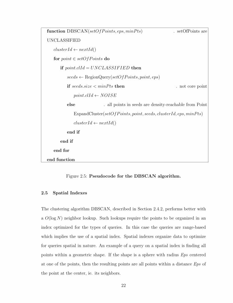
Pseudocode for the algorithm provided with the original DBSCAN paper is shown
in Figures 2.5 and 2.6. The algorithm takes values for MinPts and Eps as input and
uses that to classify every point into clusters. The algorithm runs in O(N logN)
given an O(logN) RegionQuery()[9].
Since the original paper came out, a few extensions of DBSCAN have been pub-
lished. The OPTICS algorithm[1] provides a hierarchical clustering for density-based
clusters. It generalizes away the Eps argument and only needs the MinPts parame-
ter. Another algorithm, IncrementalDBSCAN[8] significantly speeds up clustering if
most of the points have previously been clustered.
21
function DBSCAN(setOfPoints, eps,minPts) . setOfPoints are
UNCLASSIFIED
clusterId← nextId()
for point ∈ setOfPoints do
if point.clId = UNCLASSIFIED then
seeds← RegionQuery(setOfPoints, point, eps)
if seeds.size < minPts then . not core point
point.clId← NOISE
else . all points in seeds are density-reachable from Point
ExpandCluster(setOfPoints, point, seeds, clusterId, eps,minPts)
clusterId← nextId()
end if
end if
end for
end function
Figure 2.5: Pseudocode for the DBSCAN algorithm.
2.5 Spatial Indexes
The clustering algorithm DBSCAN, described in Section 2.4.2, performs better with
a O(logN) neighbor lookup. Such lookups require the points to be organized in an
index optimized for the types of queries. In this case the queries are range-based
which implies the use of a spatial index. Spatial indexes organize data to optimize
for queries spatial in nature. An example of a query on a spatial index is finding all
points within a geometric shape. If the shape is a sphere with radius Eps centered
at one of the points, then the resulting points are all points within a distance Eps of
the point at the center, ie. its neighbors.
22

function ExpandCluster(setOfPoints, point, seeds, clId, eps,minPts)
seeds.clId← clId
seeds.delete(point)
while seeds 6= ∅ do
currentP ← seeds.first()
result← RegionQuery(currentP, eps)
if result.size ≥ minPts then
for resultP ∈ result do
if resultP.clId = UNCLASSIFIED‖NOISE then
if resultP.clId = UNCLASSIFIED then
seeds.append(resultP )
end if
resultP.clID ← clId
end if
end for
end if
seeds.delete(currentP )
end while
end function
Figure 2.6: Pseudocode for the DBSCAN algorithm.
Spatial indexes are a special type of search tree. A search tree, as depicted in
Figure 2.7 is composed of nodes. Most nodes have other nodes as children (inner
nodes), but some nodes only contain data (leaf nodes). The nodes are arranged in a
way such that when searching for certain data, only some children of each node need
to be checked. In this case of the example search tree in Figure 2.7, the letter in a
node comes alphabetically after all letters stored in the subtree as its left child, and
23

Figure 2.7: Binary Search Tree example. White nodes are inner nodes. Black
nodes are leaf nodes.
alphabetically before all letters stored in the subtree as its right child.
A search is called a traversal and runs in O(logN) time. A traversal of the tree
in Figure 2.7 searching for the letter P proceeds as follows. Traversals start at the
root node of the tree, in this case M . At each step, the search letter is compared
to the letter in the node. P is compared to M , and since P comes after M in the
alphabet, the traversal moves to the node’s right child, V . Again, P is compared to
V , and since P comes before V in the alphabet, the traversal moves to the node’s left
child, R. Then, P is compared to R and since P comes before R in the alphabet, the
traversal moves to the node’s left child, P . Thus P is found after only 3 comparisons,
as opposed to 8 comparisons, one for each leaf node.
Most spatial indexes organize points by their location in a Euclidean space. This
allows for efficient queries based on the Euclidean distance d(~x, ~y) between points.
d(~x, ~y) =
√√√√ D∑i=1
(xi − yi)2
The math for Euclidean space scales to any positive number D dimensions.
Pyroprints as described in Section 2.2.3 can be thought of as ∼100 dimensional
24
points in Euclidean space. However Euclidean distances between these points would
not be comparable to Pearson correlation. Section 3.3.1 explains how we can convert
pyroprints into different ∼100 dimensional points where euclidean distances between
these points are comparable to Pearson correlation of the original pyroprints. This
allows us to store the points in normal spatial indexes in order to efficiently find points
within a certain Pearson correlation threshold.
When choosing spatial indexes for such data, the curse of dimensionality comes
in. Many spatial indexes degenerate into linear searches (searching every point) when
the points have more than a few dimensions. The following sections describe some
indexes designed specifically for high-dimensional data, while giving examples of some
simpler ones.
2.5.1 Space Partitioning
The first class of spatial indexes is space partitioning. The general case is Binary
Space Partitioning (BSP). BSP organizes data in a binary tree splitting the tree in
half with plane (or hyperplane with more dimensions) each time. As implied by the
name, each node of the tree ”partitions” the entire space.
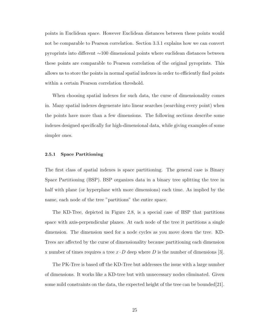
The KD-Tree, depicted in Figure 2.8, is a special case of BSP that partitions
space with axis-perpendicular planes. At each node of the tree it partitions a single
dimension. The dimension used for a node cycles as you move down the tree. KD-
Trees are affected by the curse of dimensionality because partitioning each dimension
x number of times requires a tree x ·D deep where D is the number of dimensions [3].
The PK-Tree is based off the KD-Tree but addresses the issue with a large number
of dimensions. It works like a KD-tree but with unnecessary nodes eliminated. Given
some mild constraints on the data, the expected height of the tree can be bounded[21].
25

Figure 2.8: Example KD-Tree.
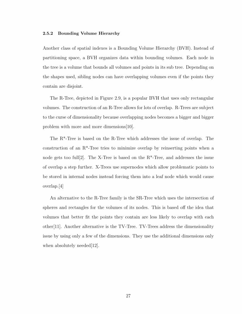
Figure 2.9: Example R-Tree.
26
2.5.2 Bounding Volume Hierarchy
Another class of spatial indexes is a Bounding Volume Hierarchy (BVH). Instead of
partitioning space, a BVH organizes data within bounding volumes. Each node in
the tree is a volume that bounds all volumes and points in its sub tree. Depending on
the shapes used, sibling nodes can have overlapping volumes even if the points they
contain are disjoint.
The R-Tree, depicted in Figure 2.9, is a popular BVH that uses only rectangular
volumes. The construction of an R-Tree allows for lots of overlap. R-Trees are subject
to the curse of dimensionality because overlapping nodes becomes a bigger and bigger
problem with more and more dimensions[10].
The R*-Tree is based on the R-Tree which addresses the issue of overlap. The
construction of an R*-Tree tries to minimize overlap by reinserting points when a
node gets too full[2]. The X-Tree is based on the R*-Tree, and addresses the issue
of overlap a step further. X-Trees use supernodes which allow problematic points to
be stored in internal nodes instead forcing them into a leaf node which would cause
overlap.[4]
An alternative to the R-Tree family is the SR-Tree which uses the intersection of
spheres and rectangles for the volumes of its nodes. This is based off the idea that
volumes that better fit the points they contain are less likely to overlap with each
other[11]. Another alternative is the TV-Tree. TV-Trees address the dimensionality
issue by using only a few of the dimensions. They use the additional dimensions only
when absolutely needed[12].
27

2.5.3 Hybrid Spatial Index
Another class of spatial index combines space partitioning and bounding volume
hierarchy. An example of this is the Hybrid-Tree. It is based on the KD-Tree but the
partitions can overlap requiring the subspaces to be treated as bounding volumes for
searching[6].
28

CHAPTER 3
DESIGN
This chapter describes the algorithms contributed along with this thesis. The al-
gorithms are the primary contribution of this thesis. The first section outlines the
goals for the solution. Next is an overview of the solution design. Following that is a
detailed look at each part of the solution.
3.1 Motivation And Goals
Chapter 2 describes the origin of the Cal Poly Library of Pyroprints (CPLOP), a
tool for a new method of Microbial Source Tracking (MST) developed by the biology
department at Cal Poly. Section 2.3 explains the benefits of identifying strains of E.
coli among the isolates stored in CPLOP.
The algorithms we contributed identify and analyze strains from the pyroprints
stored in the CPLOP. The goals for the solution were (1) to allow for faster MST,
(2) to allow strain analysis in an easy to understand form, and (3) to scale with the
database as it is incrementally updated with new pyroprints.
The ultimate purpose of this thesis is to provide an alternative solution to that
provided by Aldrin Montana in his thesis[14]. His solution, OHClust!, described
in Section 2.4.1, was motivated by the same original need, and had similar goals.
Unfortunately, the meager computational resources allocated to the CPLOP server
could not run OHClust!. As such, a secondary goal for the design of this thesis was
to have light resource requirements.
29

3.2 Overview
We started our design with the desire to try density-based clustering for strain iden-
tification to see how it compares to an agglomerative approach like OHClust! when
applied to the data collected by the biologists at Cal Poly stored in Cal Poly Library
Of Pyroprints. Many of the design decisions revolve around ensuring that we can
leverage the performance benefits of density-based clustering.
3.2.1 Speeding Up MST
The first goal for our solution was to allow for faster MST. This is very useful, because
the naive method of matching isolates for MST, comparing an unknown isolate to
every isolate in the database, scales poorly with the growing library of isolates.
As described in Section 4.8 of Jan Soliman’s thesis[20], it is possible to use iden-
tified strains to speed up the MST process. By using a representative isolate for each
strain, matching an unknown isolate only requires looking at each strain representa-
tive instead of every isolate.
This thesis contributes to this speed up by identifying strains and storing them
in CPLOP. Section 4.7.2 of Soliman’s thesis[20] describes the relational data model
for storing strains in CPLOP.
3.2.2 Allowing Strain Analysis
The second goal for our solution was to provide analysis of strains in an easy to
understand form. The purpose of analyzing bacterial strains in the library is to
find similarities between bacterial representations. These similarities signify pairs of
isolates that have some identical sequences of DNA and likely share a recent common
ancestor. This allows the biologists to look for patterns in the metadata of related
30

isolates. With metadata such as time and location of the samples, the biologists can
then ask questions like ”where has this strain of bacteria been seen?” and ”how has
that changed over time?”
OHClust! coupled the identification of strains with their analysis. As such, when
Montana was unable to verify the validity of the identified strains, the analysis could
not be used either. Hoping to avoid a similar fate, and for the sake of simplicity, we
decided to decouple strain identification and analysis in our solution. We designed
a tool that could be used to analyze strains found by any clustering method. Our
solution is to store identified strains in CPLOP, allowing researchers to use SQL
queries on CPLOP to analyze those strains.
3.2.3 Scaling With a Growing Database
The third goal for our solution is to grow with the database. The biologists are
continually gathering new samples and sequencing them into pyroprints which are
added to the database. Montana’s solution for this goal was to make OHClust!
incremental. The time to cluster a few new pyroprints in OHClust! is much faster
than clustering everything from scratch. For our solution however, we decided not to
use an incremental algorithm. This is a simpler solution that we thought would still
scale with the database due to the efficiency of the clustering algorithm we chose,
DBSCAN.
DBSCAN has a runtime complexity of O(N logN) compared to agglomerative
clustering which has complexity of up to O(N3) (as in the case of OHClust!) depend-
ing on the intercluster distance metric used. The O(N logN) complexity of density-
based clustering algorithms depends on the use of spatial indexes with O(logN) range
queries.
Spatial indexes generally operate on points in euclidean space, so in order to use
31
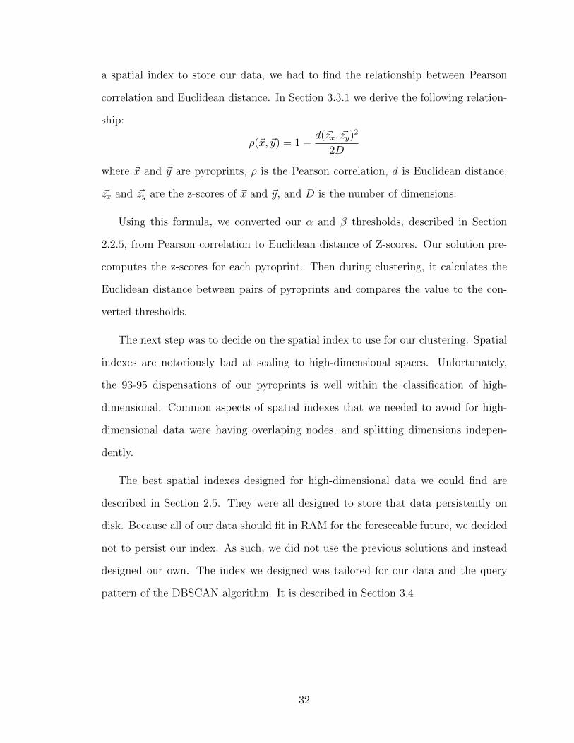
a spatial index to store our data, we had to find the relationship between Pearson
correlation and Euclidean distance. In Section 3.3.1 we derive the following relation-
ship:
ρ(~x, ~y) = 1− d(~zx, ~zy)2
2D
where ~x and ~y are pyroprints, ρ is the Pearson correlation, d is Euclidean distance,
~zx and ~zy are the z-scores of ~x and ~y, and D is the number of dimensions.
Using this formula, we converted our α and β thresholds, described in Section
2.2.5, from Pearson correlation to Euclidean distance of Z-scores. Our solution pre-
computes the z-scores for each pyroprint. Then during clustering, it calculates the
Euclidean distance between pairs of pyroprints and compares the value to the con-
verted thresholds.
The next step was to decide on the spatial index to use for our clustering. Spatial
indexes are notoriously bad at scaling to high-dimensional spaces. Unfortunately,
the 93-95 dispensations of our pyroprints is well within the classification of high-
dimensional. Common aspects of spatial indexes that we needed to avoid for high-
dimensional data were having overlaping nodes, and splitting dimensions indepen-
dently.
The best spatial indexes designed for high-dimensional data we could find are
described in Section 2.5. They were all designed to store that data persistently on
disk. Because all of our data should fit in RAM for the foreseeable future, we decided
not to persist our index. As such, we did not use the previous solutions and instead
designed our own. The index we designed was tailored for our data and the query
pattern of the DBSCAN algorithm. It is described in Section 3.4
32

3.3 Isolate Comparison
There are two components to comparing isolates. First is the comparison of pyroprints
from the same DNA region. Second is the way comparisons from all DNA regions are
used to come to a decision on similarity.
3.3.1 Euclidean Distance of Pyroprint Z-Scores
Spatial indexes generally operate on data existing in Euclidean space. The pyroprints
could be thought of as points in an D-dimensional space where D is the number of
dispensations. The distance between two points in Euclidean space can’t be converted
to the Pearson correlation between two points which was previously used by those
working with CPLOP. The calculation of the Pearson correlation uses the average
and standard deviation of the dimensions in a point, but Euclidean distance discards
the information needed to find the average and standard deviation. There is a type
of spatial indexes called a m-tree which can operate on arbitrary metrics[16]. Unfor-
tunately, the Pearson correlation does not fit the criteria of a proper metric which is
required by m-trees. Specifically, Pearson correlation violates the triangle inequality
property.
The reason the biologists use Pearson correlation, as described in Section 2.2.4, is
because it statistically normalizes the data. We needed Euclidean distance for use in a
spatial index, and we needed to use statistical normalization for comparison validity.
Since the biologists had already determined meaningful thresholds for Pearson corre-
lation, we hoped to be able to leverage that by finding a relationship between Pearson
correlation and Euclidean distance with statistical normalization. The following is a
derivation of that relationship.
33

We start with the equations for Pearson correlation ρ and Euclidean distance d:
ρ(~x, ~y) =1
D
D∑i=1
(xi − µx)(yi − µy)σxσy
d(~x, ~y) =
√√√√ D∑i=1
(xi − yi)2
where D is the number of dimensions, and µx and σx are the mean and standard
deviation respectively.
µx =1
D
D∑i=1
xi
σx =
√√√√ 1
D
D∑i=1
(xi − µx)2
We notice that the inner terms of Pearson correlation are z-score normalizations,
z(xi) =xi − µxσx
and plug in z(xi) into the distance equation for x and y and simplify.
d(~zx, ~zy) =
√√√√ D∑i=1
(xi − µxσx
− yi − µyσy
)2
=
√√√√ D∑i=1
(xi − µxσx
)2
− 2
(xi − µxσx
)(yi − µyσy
)+
(yi − µyσy
)2
=
√√√√( D∑i=1
(xi − µxσx
)2)
+
(D∑i=1
(yi − µyσy
)2)− 2
D∑i=1
(xi − µxσx
)(yi − µyσy
)
=
√√√√∑(xi − µx)2σx2
+
∑(yi − µy)2σy2
− 2D∑i=1
(xi − µx)(yi − µy)σxσy
We notice the the sums look like parts of the equations for σ and ρ. Solving the
equations for the sums gives us:
D∑i=1
(xi − µx)2 = D · σx2
D∑i=1
(xi − µx)(yi − µy)σxσy
= D · ρ(~x, ~y)
34

ITS region 23-5 16-23α β α β
ρ(~x, ~y) 0.995 0.99 0.995 0.99
D 93 95d(~zx, ~zy) 0.9644 1.3682 0.9747 1.3784
Table 3.1: Converted Thresholds.
and we substitute those back into our d(~zx, ~zy) equation and simplify.
d(~zx, ~zy) =
√D · σx2σx2
+D · σy2σy2
− 2D · ρ(~x, ~y)
=√
2D − 2D · ρ(~x, ~y)
=√
2D(1− ρ(~x, ~y))
Thus the relationship between ρ and d is:
d(~zx, ~zy) =√
2D(1− ρ(~x, ~y))
or
ρ(~x, ~y) = 1− d(~zx, ~zy)2
2D
Using this formula, we converted our α and β thresholds from Pearson correlation
to Euclidean distance of Z-scores, shown in Table 3.1. Because the conversion depends
on number of dimensions D, the threshold for distance is different for each region
despite being the same for Pearson correlation.
Our solution precomputes the z-scores for each pyroprint. Then during clustering,
it calculates the Euclidean distance between pairs of pyroprints and compares the
value to the converted thresholds.
35
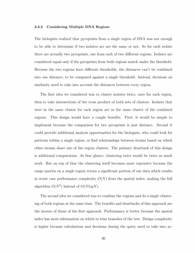
3.3.2 Considering Multiple DNA Regions
The biologists realized that pyroprints from a single region of DNA was not enough
to be able to determine if two isolates are are the same or not. So for each isolate
there are actually two pyroprints, one from each of two different regions. Isolates are
considered equal only if the pyroprints from both regions match under the threshold.
Because the two regions have different thresholds, the distances can’t be combined
into one distance, to be compared against a single threshold. Instead, decisions on
similarity need to take into account the distances between every region.
The first idea we considered was to cluster isolates twice, once for each region,
then to take intersections of the cross product of both sets of clusters. Isolates that
were in the same cluster for each region are in the same cluster of the combined
regions. This design would have a couple benefits. First, it would be simple to
implement because the comparison for two pyroprints is just distance. Second it
could provide additional analysis opportunities for the biologists, who could look for
patterns within a single region, or find relationships between strains based on which
other strains share one of the region clusters. The primary drawback of this design
is additional computation. At first glance, clustering twice would be twice as much
work. But on top of that the clustering itself becomes more expensive because the
range queries on a single region return a significant portion of our data which results
in worst case performance complexity O(N) from the spatial index, making the full
algorithm O(N2) instead of O(NlogN).
The second idea we considered was to combine the regions and do a single cluster-
ing of both regions at the same time. The benefits and drawbacks of this approach are
the inverse of those of the first approach. Performance is better because the spatial
index has more information on which to trim branches of the tree. Design complexity
is higher because calculations and decisions during the query need to take into ac-
36
count two independent regions. This also means that the query algorithm takes two
radii as input, one for each region, instead of the normal one radius.
We decided to use the second approach for this work. While the opportunity for
extra analysis would be nice, it wasn’t specifically asked for, while good performance
was. Additionally, the analysis would likely be performed infrequently, and thus the
extra computation would be wasted most of the time. Perhaps in the future the ability
to make such analyses could be added separately from the basic strain identification.
3.4 Spatial Index
All of the design for strain identification revolved around the spatial index. The data
was transformed into z-scores and the thresholds converted for Euclidean distance
so that a spatial index could be used. Density-based clustering gets its performance
from leveraging a spatial index.
Our primary concern with choosing a spatial index is the fact that our data is high-
dimensional. Most spatial indexes scale poorly with dimensions. Common aspects
of spatial indexes that we needed to avoid for high-dimensional data were having
overlapping nodes, and splitting dimensions independently.
The best spatial indexes designed for high-dimensional data we could find are
described in Section 2.5. They were all designed to store that data persistently on
disk. Because all of our data should fit in RAM for the foreseeable future, we decided
not to persist our index. As such, we did not use the previous solutions and instead
designed our own.
Because we decided not to have a persistent index, it must be built from scratch
whenever we want to cluster the data. Therefore, we must choose a spatial index
which can be built quickly. Specifically, the complexity should not be worse than the
37

complexity of the clustering, O(N logN), otherwise building the tree would dominate
the total runtime as the dataset scales.
Designing our own spatial index allows us to make some optimizations for its use
in DBSCAN as well as for the specific characteristics of our data.
3.4.1 Optimizations for use with DBSCAN
In order to be used by DBSCAN, the spatial index needed to provide a range query.
A range query takes a query point, and a range as input and returns all data points
within range of the query point. The query can be thought of as a hypersphere with
it’s center at the query point with a radius of the query range. All points that lie
inside that hypersphere are returned.
The DBSCAN algorithm queries the spatial index in a unique pattern. First, all
queries are centered at a point in the database, as opposed to an arbitrary point
with all queries having the same range. Second, each point is only queried once, and
nearby points are processed soon after each other.
Our spatial index query takes some shortcuts by realizing that once a point and
all of its neighbors have been processed, DBSCAN will never make another query
that would return that point. In addition, we modified the DBSCAN algorithm to
keep track of the neighbors seen for each unprocessed point. This means that it will
never need to see any points more than once. These modifications are described in
Section 3.5.1.
By only committing to returning points that have not been previously returned we
can get away with only searching points that haven’t been returned yet. By removing
points from the spatial index after they are returned, future queries will have fewer
points to search through.
38

[0.0, 0.25) [0.25, 0.5) [0.5, 0.75) [0.75, 1.0) [1.0, 1.25) [1.25,∞)
23-5 37 45 7 0 3 116-23 46 39 6 1 0 2
Table 3.2: Number of dimensions with a standard deviation in various
ranges for each ITS region. The deviations are calculated between z-scores, not
the original pyroprints.
3.4.2 Data Characteristics
Our data has some characteristics that make it difficult to use in a spatial index. The
points have very little spread in most dimensions. As shown in Table 3.2, standard
deviations between points in a single dimension are less than 0.5 for most dimensions.
Compared to the range of the query of 0.96 or 0.97 for the α thresholds of 23-5 and
16-23 respectively, the difference between points in a single dimension usually won’t
be enough to exclude a point from the query results. Unfortunately, we can’t ignore
any single dimension because those small differences add up over ∼100 dimensions.
Unfortunately, this means that when traversing the tree, the algorithm will branch
to multiple children to a greater depth, until many dimensions have been looked at.
In order to keep the tree depth low, our design splits points based on multiple
dimensions per level. This is common in spatial indexes such as the popular quadtree
and octree, however, that approach increases the number of children of each node
exponentially (2D) where D is the number of dimensions split at that level. Splitting
all ∼100 dimensions in one node would be impractical with 290 children. We could
instead split only a few different dimensions at each level of the tree, but the tree
would still have the same number of leaves after splitting each dimension once. Since
290 leaves is more than the number of data points we could ever possible hope to add
to the database, the majority of those leaves would be wasted. In addition, the range
39

query would intersect many of these children, causing the algorithm to traverse down
exponentially many paths. This is somewhat offset by the reduced depth of the tree,
but it is not ideal. The O(logN) performance of spatial data queries assumes that at
the majority of nodes, only one child is further traversed.
What we decided to do instead was split multiple dimensions dependently. That
is to split once but have that one split cover multiple dimensions. This means that the
split plane won’t be axis aligned. The idea is that by changing the angle of the split
plane the average distance from points on either side to the split plane will increase.
This increase depends on a correlation between dimensions i.e. points with low values
(relative to other points) in one dimension, also tend to have low values (relative to
other points) in another dimension. Inverse correlations work too, as long as most
points with low values in one dimension have high values in another. Fortunately, the
data in our library does exhibit correlations between some dimensions.
3.4.3 Construction
This section describes the remaining details of the design of the spatial index. Since
the tree is not persistent, we can construct the tree with knowledge of all the points.
Instead of constructing the tree by adding one point at a time and splitting nodes
when they get too big (like many bounding volume hierarchy indexes) or picking
arbitrary split criteria ahead of time (like many spatial partitioning indexes), our
design looks at all points in a (sub)tree then partitions them.
As discussed in Section 3.4.2, our spatial index partitions points by finding a plane
that splits the data in multiple correlated dimensions. The dimensions are chosen by
picking the single dimension in which the points are most spread apart, as determined
by standard deviation, and then choosing a number of other dimensions based on a
combination of how correlated they are to the first dimension and how spread those
40

dimensions are. Specifically it chooses the N dimensions with the highest values for
|ρ|·σ, where ρ is the Pearson correlation of data values for a dimension with the values
for the dimension with the most spread, σ is the standard deviation for a dimension,
and N is a parameter to the construction algorithm.
Each dimension is only split once per path down the tree. The true distance to
a node is not simply the distance to the split plane of that node, but actually the
distance to the intersection of the planes of all the ancestors of the node. Instead
of finding those intersections and calculating the distance to the complex shape that
results, we can combine the distances to individual planes using Euclidean distance
dcombined =√d1
2 + d22. In order to combine distances from multiple split planes
during queries (the split planes from a node and all of its ancestors), each of those
planes must be perpendicular to all of the others. The simplest way to guarantee this
is to enforce that no plane shares any dimension with another. Dimensions will be
reused in the planes of nodes that aren’t direct ancestors or descendants as distances
to those planes will not be combined during queries.
After picking the dimensions, our construction algorithm chooses a hyper-plane
using linear regression between each dimension and the dimension with the most
spread. The formula determines the slope b = ρ · σxσy
and intercept i = sx − b · sy of
the regression line a · x+ b · y+ i = 0 where x is the value of a point in the dimension
with greatest spread, y is the value of the point in the other correlated dimension, and
a := 1. The intercept i determines the position of the split plane, and is calculated for
a point s on the plane. We tried two options for s, the mean of each dimension, and
the median point in relation to the split plane. The mean is less work to calculate,
thus results in faster construction. The median point results in a balanced tree, thus
faster queries. Since the performance of our spatial index is dominated by the queries
and not the construction, we chose to use the median point.
41

The algorithm finds an equation of a hyper-plane by combining these linear re-
gression equations into a form a ·x+ b · y+ . . .+ c · z+ i = 0 where x is the dimension
with the most spread (again with a := 1) and each subsequent term is a correlated
dimension multiplied by the slope (b · y) of the linear regression with the first dimen-
sion. The intercept i is simply the sum of the intercepts from the linear regression
for each correlated dimension.
In order to partition the points based on the hyper-plane, we needed a function
that, given a point < x0, y0, · · · , z0 > and the equation for the plane (a · x + b · y +
. . . + c · z + i = 0), would return which side of the plane it was on. We used the
equation for signed distance from a plane for this purpose as well as for the spatial
query algorithm. The formula for the distance is
d =a · x0 + b · y0 + . . .+ c · z0 + i√
a2 + b2 + . . .+ c2
The result of this equation is signed, and that sign determines which side of the plane
a point is on. For the purpose of partitioning, only the sign matters, so we can ignore
the denominator. Since the plane is only in a subset of the dimensions, the ”point”
we input to the function is made up of only those dimensions from the real data point,
in the same order as they are used in the plane equation.
3.4.4 Storage
After deciding which points go in which child of a tree node, the algorithm has to
encode spatial information about those children for the query to use. The two most
common methods of doing this are (1) storing the plane used to split the data i.e.
spatial partitioning, and (2) storing a bounding volume for each child fit to the data
points within i.e. bounding volume hierarchies. The benefits of storing the split plane
are that it generally takes less storage space, and it guarantees no overlap between
children which can be a problem with bounding volumes. Bounding volumes come
42
in many shapes and sizes each with different characteristics, however in general, they
take more storage space and the better they fit the data, the more complex the
comparisons or construction.
We tried both methods for our data, storing the plane as used during construction
and storing axis-aligned bounding boxes for each child. We chose axis aligned bound-
ing boxes for the simplicity of construction and comparison. However, axis-aligned
boxes generally suffer from empty corners and in our case, since the points aren’t
split by axis-aligned planes, those corners could cross over the split plane, making
overlapping children probable. Comparison against bounding spheres would also be
fairly simple and would avoid empty corners, however they lose that simplicity when
scaled in different dimensions, becoming ellipses. Since our data is very skewed, and
since by the nature of spatial partitioning, the data would become more skewed in
lower levels in the tree, using uniform spheres could result in good fit in the most
spread dimensions but lots of extra space on the sides of other dimensions. These
hypotheses were not tested, but the choice of axis aligned bounding boxes was mostly
driven by simplicity of construction. Constructing a minimum bounding sphere is not
nearly as simple as constructing a minimum axis aligned bounding box
Comparing a query range against split planes was more effective than axis aligned
bounding boxes at higher levels in the tree closer to the root. However, deeper into the
tree, the effectiveness of the methods swapped, and the axis aligned bounding boxes
were better at pruning children. This complementary behaviour led to our decision to
use both methods of storage. We considered storing only planes at higher levels and
only bounding boxes at lower levels, however we theorized that extra discrimination
and thus less branching at each level was more important than reduced node storage
and comparison time. This could be something to try in future work.
All of the previous design details involve only a single ITS region. The addition of
43

more regions does not affect the design of a single region. While we made an effort to
retain a binary split for a single region by combining multiple dimensions in a single
split plane, we don’t do this for multiple regions. Because of the inability to combine
distances from multiple regions described in Section 3.3.2, we instead decided to add
more children.
For example, with two regions we would have two split planes. Each split plane
uses whichever dimensions it wants (there is no connection between any dimensions
from one region and another). They don’t even need to use the same number of
dimensions, each plane is completely independent. For two regions there will be 4
children like a quad tree. One child is for points with a negative distance to the planes
for both regions. Another child is for points with a positive distance to both. The
other two children are for points with a positive distance to one region’s plane and a
negative one to the other.
3.4.5 Algorithms
Pseudocode for our tree construction algorithm is shown in Figure 3.1. It’s a recursive
algorithm that constructs and returns subtrees of the spatial index. The base case
is determined by the number of points passed to the algorithm. If the number of
points (isolates) passed to the algorithm is less than POINTS PER LEAF variable,
it constructs a new leaf node with those points and returns it. In the general case the
algorithm partitions the points and calls the algorithm recursively to create children
nodes used to construct an inner node which is then returned. Points are partitioned
according to the scheme described in Section 3.4.3 with a plane perpendicular to the
linear correlation between a number of dimensions defined by DIMS PER SPLIT.
Figures 3.2, 3.3 and 3.4 contain pseudocode for the range query algorithm. This
algorithm is also recursive, returning the set of previously unseen points within radius
44
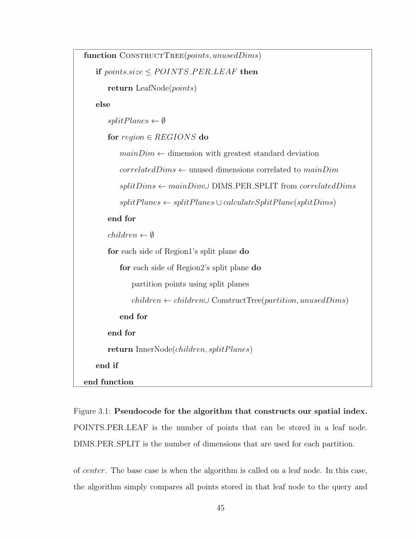
function ConstructTree(points, unusedDims)
if points.size ≤ POINTS PER LEAF then
return LeafNode(points)
else
splitP lanes← ∅
for region ∈ REGIONS do
mainDim← dimension with greatest standard deviation
correlatedDims← unused dimensions correlated to mainDim
splitDims← mainDim∪ DIMS PER SPLIT from correlatedDims
splitP lanes← splitP lanes ∪ calculateSplitP lane(splitDims)
end for
children← ∅
for each side of Region1’s split plane do
for each side of Region2’s split plane do
partition points using split planes
children← children∪ ConstructTree(partition, unusedDims)
end for
end for
return InnerNode(children, splitP lanes)
end if
end function
Figure 3.1: Pseudocode for the algorithm that constructs our spatial index.
POINTS PER LEAF is the number of points that can be stored in a leaf node.
DIMS PER SPLIT is the number of dimensions that are used for each partition.
of center. The base case is when the algorithm is called on a leaf node. In this case,
the algorithm simply compares all points stored in that leaf node to the query and
45

function RangeQuery(node, center, radii)
result← ∅
switch typeof(node) do
case leafNode
for point ∈ leafNode.points do
if PointInSpheres(point, center, radii) then
result← result ∪ point
remove point from leafNode.points
end if
end for
end case
case innerNode
for childNode ∈ innerNode.children do
if NodeIntersectsSpheres(innerNode, center, radii) then
result← result∪ RangeQuery(childNode, center, radius)
end if
end for
end case
end switch
return result
end function
Figure 3.2: Pseudocode for our range query algorithm.
returns those that match. In the general case, the algorithm is called on an inner
node. The algorithm first determines which nodes might possibly contain points that
match the query. Then it recursively calls the algorithm on each of those children
and combines the results.
46

function PointInSpheres(point, center, radii)
for region ∈ REGIONS do
radius← radii[region]
if distance(center[region], point[region]) ≥ radius then
return False
end if
end for
return True
end function
Figure 3.3: Pseudocode for our range query algorithm.
function NodeIntersectsSpheres(node, center, radii)
for region ∈ REGIONS do
planeDist← PlaneDistance(center[region], child.planes[region])
bboxDist← BBoxDistance(center[region], child.bboxes[region])
if max(planeDist, bboxDist) ≥ radii[region] then
return False
end if
end for
return True
end function
Figure 3.4: Pseudocode for our range query algorithm.
3.5 Clustering
The primary reason we chose to use density-based clustering was that it is different
from agglomerative clustering. Of course, there are other clustering methods which
47
are different from agglomerative clustering, but density-based clustering offers better
performance and cluster determinism independent of input order. We had to decide
on a specific density-based clustering algorithm from among the options described in
Section 2.4.2.
A hierarchical clustering algorithm could provide extra information for strain anal-
ysis. If isolates in one strain are more similar to each other than isolates in another
strain, a dendrogram would reflect that. However, generating that dendrogram would
come at the cost of performance. The hierarchical density-based clustering algo-
rithm, OPTICS, is more demanding of the spatial index. It requires finding the
distance to the minPtsth closest neighbor for each point instead of just the number
of points within the range. Nearest neighbor searches can actually be faster than
radius searches. However, to get the benefit of hierarchical clusters, the max search
radius would need to be bigger than the radius we would use for normal DBSCAN,
ending up with a net decrease in performance. Finally, finding the nearest neighbors
requires sorting points based on their distance to the query point. However, as men-
tioned in 3.3.2, we cannot combine the distances from multiple DNA regions into one
distance, meaning we would have to cluster each region separately. Because these
new analysis opportunities were not specifically requested and performance was, we
decided OPTICS was not worth the tradeoff and to use DBSCAN instead. Perhaps in
the future, the team could add a standalone tool using OPTICS on individual regions
for infrequent analysis.
Due to the inherent performance gains from switching to a lower algorithmic
complexity, we decided that using an incremental algorithm was not worth the added
responsibility of persisting internal algorithm information and maintaining a list of
new or removed data points between clustering runs. An algorithm with complexity
O(N logN) can scale well with a growing dataset. Upgrading to an incremental
version could be a good avenue for future work.
48
3.5.1 Modified DSBCAN Algorithm
In order to take advantage of the shortcut discussed in Section 3.4.1, we needed to
modify the original DBSCAN algorithm. Our spatial index query deletes points as it
returns them, meaning it only returns points that have not been previously seen. In
some cases, this works with the unmodified DBSCAN algorithm, however we had to
modify the algorithm to handle the edge cases.
When a point is processed by the standard DBSCAN algorithm, the spatial index
is queried for the Eps-neighbors of the point. If the number of neighbors for a point
is at least minPts then the point and its neighbors are added to the current cluster
(creating a new cluster if there isn’t one). Then, the algorithm adds each neighbor
to a seeds list. Once a point is done being processed, another point is taken from
the seeds list and that point is processed. If the seeds list is empty, then the current
cluster is completed and the next point to be processed is taken from the set of all
points. When a point is processed, there are two possibilities: Either it is processed
in the outer DBSCAN() function, or in the inner ExpandCluster() function.
If a point is processed in the inner ExpandCluster() function, then by definition
at least one of its neighbors has been seen and the point is being added to a cluster.
We could compensate for this by simply adding one to the points neighbor count,
but there are two edge cases here. First it is possible that (1) the point could have
other neighbors in the same cluster which were already processed. Second, (2) some
of the point’s other neighbors could have be seen by another point in the cluster. In
both cases, the neighbor in question would have been removed from the spatial index
before this point was processed. Neither of these edge cases affect whether or not the
point will be added to the cluster, but the count of neighbors does affect whether the
point’s previously unseen neighbors will also be added to the cluster.
If instead a point is processed in the outer DBSCAN() function, it generally means
49

that the point is not a neighbor of any points that have previously been seen; otherwise
it would have likely been added to seeds and queried from ExpandCluster() instead.
This means that the set of previously unseen neighbors is the same as the set of all
neighbors. The edge case here is that (3) one of the point’s neighbors could have
been seen by a non-core point. When this happens, the neighbor would have been
removed from the spatial index but not added to seeds (where it would have queried
the point instead of the other way around).
The first modification we made is that the algorithm now maintains for each
unprocessed point, a list, seenNeighbors of all the processed points who have seen
that point. Then, when a point is processed, the number of points in seenNeighbors
is added to the number of previously unseen neighbors returned by the spatial query.
This combined count is used to determine whether the point is a core point, and if
the combined count is at least minPts, the unseen neighbors are added to seeds like
normal, as well as all of the already seen neighbors (which may or may not already be
in that cluster). Then the algorithm adds the processed point to the seenNeighbors
for each of the previously unseen points. By itself, this modification doesn’t fix any
of the edge cases, as it only accounts for the one neighbor which first saw each point,
but it serves as a platform to address them.
The next modification is that when a point is processed, in addition to querying
the spatial index, the point is compared to every other point in seeds. For each
seed point within eps of the point being processed, the algorithm adds both the seed
point and the point being processed to each other’s seenNeighbor. This modification
mostly solves edge cases 1 and 2. However, the modification itself has an edge case
where (4) one of the point’s neighbors could have been seen by a non-core point.
When this happens, the neighbor would have been removed from the spatial index
but not added to seeds (where it would have been found during this modified point
processing).
50

Edge cases 3 and 4 are actually the same problem surfacing in different spots,
and are related to another concern that removing points from the spatial index could
result in some points never being processed. This could happen if a point was seen
by a non-core point in which case it would not have been added to seeds, but was
still deleted from the spatial index. If the spatial index is the source of unprocessed
points used by the outer DBSCAN() function, then the point will never be queried.
We considered two solutions to this problem. The first solution was to decouple
the removal of points in the spatial index from the query, and instead only remove
points if the point being processed turns out to be a core-point (and thus the removed
points will be added to seeds. The second solution was to keep points that have been
seen by non-core points in a noise list like seeds but separate. Then when points are
being processed the algorithm would compare the point to each of the points in noise,
in addition to those in seeds. We chose to use the noise list because it removes points
from the spatial index as soon as possible, hopefully speeding up future queries.
Pseudocode for our modified DBSCAN algorithm is in Figures 3.5 and 3.6. For
reference, the pseudocode for the original DBSCAN can be found in Figure 2.5 and
2.6.
51

function ModifiedDBSCAN(setOfPoints, eps,minPts)
. setOfPoints are UNCLASSIFIED
while setOfPoints 6= ∅ do
point← setOfPoints.pop()
neighbors← RegionQuery(setOfPoints, point, eps)
if neighbors.size ≥ minPts then . all neighbors are density-reachable
clId← nextId()
point.clId← clId
neighbors.clId← clId
noise← ∅
seeds← neighbors
else . not core point
clId← −1 . not currently expanding a cluster
noise← neighbors
seeds← ∅
end if
ExpandNeighbors(setOfPoints, point, seeds, noise, clId, eps,minPts)
end while
end function
Figure 3.5: Pseudocode for our modified DBSCAN algorithm.
52

function ExpandNeighbors(unseen, point, seeds, noise, clID, eps,minPts)
update seenNeighbors
while seeds 6= ∅‖noise 6= ∅ do
if seeds 6= ∅ then
point← seeds.pop()
else
clId← −1 . not currently expanding a cluster
point← noise.pop()
end if
neighbors← RegionQuery(unseen, point, eps)
update seenNeighbors
if neighbors.size+ seenNeighbors[point].size ≥ minPts then
if clID = −1 then
clId← nextId()
point.clId← clId
end if
move any seenNeighbors[point] from noise to seeds
seeds = seeds ∪ neighbors
neighbors.clId← clId
seenNeighbors[point]← clId
end if
end while
end function
Figure 3.6: Pseudocode for our modified DBSCAN algorithm.
53
CHAPTER 4
IMPLEMENTATION
This chapter describes the implementation of the work contributed with this thesis.
It is intended to serve as a reference for researchers using this work for future work.
The code is accessible from a github repository1.
4.1 Language and Libraries
We implemented the work in Python, and utilized a few third party libraries. We
ran the evaluations with version 3.4.3, but the code should be compatible with any
version 3.X of python. We chose Python originally just to prototype the solution. We
were happy with the performance of the libraries though, so when we went to create
the final implementation we stuck with the same language.
A couple of the packages we used are from the open source library SciPy2. SciPy
is a collection of software packages for math, science, and engineering. We used
version 0.14.0. For evaluating clusters, we used the Statistics package (stats). The
Statistics package provides objects representing statistical distributions and methods
for analysing and comparing random samples or distributions. We used NumPy for
storing and comparing pyroprints. NumPy provides N-dimensional array objects and
efficient vector operations on those arrays. NumPy is maintained by SciPy but is
available standalone, with it’s own versions. We used version 1.8.1.
In order to interface with CPLOP, which is implemented as a MySQL database, we
used the MySQL Connector provided by MySQL3. MySQL Connector, like MySQL
1https://github.com/ejohns32/Thesis-Code2http://www.scipy.org/install.html3http://dev.mysql.com/downloads/connector/python/
54

is open source. MySQL connector handles connecting to and querying a MySQL
database. It also handles data conversion into standard Python types. We used
version 2.0.3.
Python and all of the libraries we used are available together through Anaconda.
Anaconda is a package manager and Python distribution available from Continuum
Analytics4. This is what we used, although newer versions will come with up to date
Python and libraries that may be incompatible with this code.
4.2 Overview
This section describes how the different modules of the implementation interface with
each other. It does this in the context of a typical run of the program.
First the implementation loads settings from a configuration file. These settings
are described in the sections detailing each module. The configuration file includes
descriptions of each ITS region which are represented by Region objects.
In the pyroprinting module, the program queries pyroprints from CPLOP us-
ing the mysql.connector library. The pyroprints are then organized and stored as
Isolate objects. The Isolate class provides an isWithinRadiiOf() function which
takes another Isolate and a radius for each Region returning a boolean value.
In the spatial and fullsearch modules, the implementation takes a list of
Isolates and constructs a SpatialIndex or FullSearchIndex respectively. SpatialIndex
and FullSearchIndex both provide a getNeighborsOf() and popNeighborsOf()
function, which both take an Isolate and a radius for each region. The functions
return the set of Isolates for which the isWithinRadiiOf() function returns true.
The dbscan module contains two functions for creating clusters: dbscan() and
4https://www.continuum.io/downloads
55

popDBSCAN() which both take an Index and DBSCAN’s eps and minPts parameters.
The functions call the getNeighborsOf() and popNeighborsOf() functions of the
passed Index respectively to determine clusters. The functions both return a list of
clusters, each cluster represented as a set of Isolates.
The clusterEval module is optional. It provides functions which evaluate one or
more lists of clusters as returned by the functions in the dbscan module.
4.3 Data Types
The Region class, defined in module pyroprinting, contains information about a sin-
gle ITS region. Instances are created from the configuration file. The class contains
fields for the name of the ITS region, the dispensation count, a Pearson correlation
similarity threshold (which is converted to zScore distance and used as eps for DB-
SCAN), and parameters for the beta distribution of Pearson correlations between
pyroprint regions of the same strain.
The Isolate class, defined in module pyroprinting, aggregates one pyroprint
from each ITS region. Pyroprints are stored as numpy.arrays of zScores. The class
provides functions for comparing its pyroprints to those of other isolates, namely
isWithinRadiiOf(). Isolates are obtained by querying CPLOP for pyroprints.
The query we used is in Figure 4.1. The query grabs the latest pyroprint from each
region. After the query, we also filter out isolates which don’t have pyroprints for
both regions.
The BoundingBox class, defined in module spatial, represents an N-dimensional
axis aligned bounding box, where N is the number of dispensations for the ITS region
it encloses. It is stored as two numpy.arrays, one contains the minimum values for
each dispensation of every pyroprint contained in the bounding box, and the other
contains the maximum values for each dispensation.
56
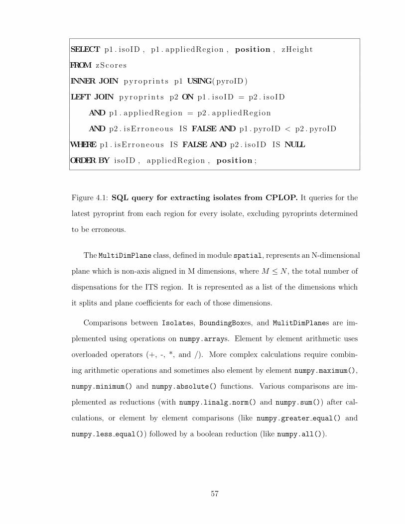
SELECT p1 . isoID , p1 . appl iedRegion , position , zHeight
FROM zScore s
INNER JOIN pyropr in t s p1 USING( pyroID )
LEFT JOIN pyropr in t s p2 ON p1 . i soID = p2 . i soID
AND p1 . appl iedRegion = p2 . appl iedRegion
AND p2 . i sErroneous IS FALSE AND p1 . pyroID < p2 . pyroID
WHERE p1 . i sErroneous IS FALSE AND p2 . i soID IS NULL
ORDER BY isoID , appl iedRegion , position ;
Figure 4.1: SQL query for extracting isolates from CPLOP. It queries for the
latest pyroprint from each region for every isolate, excluding pyroprints determined
to be erroneous.
The MultiDimPlane class, defined in module spatial, represents an N-dimensional
plane which is non-axis aligned in M dimensions, where M ≤ N , the total number of
dispensations for the ITS region. It is represented as a list of the dimensions which
it splits and plane coefficients for each of those dimensions.
Comparisons between Isolates, BoundingBoxes, and MulitDimPlanes are im-
plemented using operations on numpy.arrays. Element by element arithmetic uses
overloaded operators (+, -, *, and /). More complex calculations require combin-
ing arithmetic operations and sometimes also element by element numpy.maximum(),
numpy.minimum() and numpy.absolute() functions. Various comparisons are im-
plemented as reductions (with numpy.linalg.norm() and numpy.sum()) after cal-
culations, or element by element comparisons (like numpy.greater equal() and
numpy.less equal()) followed by a boolean reduction (like numpy.all()).
57

4.4 Indexes
The SpatialIndex class, defined in module spatial, is an implementation of the
data structure designed for this thesis and described in Section 3.4. It provides a
getNeighborsOf() and popNeighborsOf() function, which both take an Isolate
and a radius for each region. The functions return the set of Isolates for which
the isWithinRadiiOf() function returns true. An instance is constructed from a list
of Isolates. The construction algorithm uses some settings from the configuration
file which affect when leaf nodes will be built, or how many dimensions will be used
for MultiDimPlanes. A SpatialIndex is composed of Nodes which are themselves
composed of SpatialFilters and either other Nodes or Isolates.
The SpatialFilter class is a generic representation of methods for determining if
any points in subtree might match the neighbor query. These methods are associated
with Nodes in the SpatialIndex, and are specific to a single ITS region, meaning there
can be one SpatialFilter per filter method per ITS region per Node. Currently we
have 2 methods and 2 ITS regions for a total of 4 SpatialFilters per Node. The
SpatialFilter class is an abstract class providing basic functionality for connecting
SpatialFilters from one Node to the corresponding (same ITS region and method)
SpatialFilters from the Node’s parent and children. It is intended to be extended
for each filtering method with an intersectsQuery() function for checking if a query
intersects with the filter, and an update() / aggregrate() function for updating the
filter when points are removed from the subtrees of the LeafNode / InnerNode the
filter is associated with.
The first filtering method is represented by the PlanePartitionFilter class
which extends the SpatialFilter class. These filters represent a method of fil-
tering using the MultiDimPlanes used to partition points during construction. Its
intersectsQuery() function calculates the distance to the MultiDimPlane associ-
58

ated with the filter, and those of all of filters ancestors. The implementation uses the
cached result from parent to speed up its calculation. Then it caches its result for
use by its children. Its update() and aggregrate() are no-ops because updating the
MultiDimPlane implies updating the partition. We would have liked to implement
repartitioning the points to rebalance the spatial index, however we decided to leave
this for future work.
The second filtering method uses the BoundingBoxFilter class which also extends
the SpatialFilter class. These filters represent a bounding volume hierarchy with
axis aligned bounding boxes. Its intersectsQuery() function calculates the distance
to the BoundingBox associated with the filter. Its update() function updates its
BoundingBox to fit the reduced set of points contained by the LeafNode it is associated
with. The aggregrate() function updates its BoundingBox to fit those of its children
filters.
Node is an abstract class which implements the common functionality of InnerNodes
and LeafNodes. The Node class manages the SpatialFilters and logic for determin-
ing if the subtree starting at the Node might contain points matching the query. It
provides a intersectsQuery() function which is used by the InnerNode class to
determine of the query traversal can ignore the Node. The intersectsQuery() calls
the intersectsQuery() function of each of its SpatialFilters, and takes advan-
tage of short circuiting to avoid the expensive caculations of the SpatialFilters
high-dimensional pyroprint comparisons.
The InnerNode class extends Node and represents a node of the search tree which
contains other Nodes instead of points. This class implements the search traversal
logic which decides which of its children Nodes to continue searching.
The LeafNode class extends Node and represents a terminating node in the search
tree. It contains Isolates (or any other object with a isWithinRadiiOf() function).
59
This class contains the logic which ultimate decides if a point will be returned and
deletes the points it does return.
The FullSearchIndex class, defined in module fullsearch, is an implementation
of a naive index. Neighbor lookups search every isolate which is O(N) instead of the
O(N logN) of the spatial index. This naive implementation has the same interface as
SpatialIndex, constructed with a list of Isolates and exposing getNeighborsOf()
and popNeighborsOf() functions. This implementation serves as a benchmark for
performance testing SpatialIndex.
The PrecomputedIndex class, defined in module fullsearch, is another imple-
mentation of an index. This index is constructed with a map from every isolate to
the set of isolates which are neighbors of that isolate. The neighbor lookup is O(1),
however the precomputation is as expensive as running a neighbor lookup once for
every isolate in one of the other indexes. Because the precomputation only needs to
be ran once, this index is useful for trying out different clustering parameters quickly.
4.5 DBSCAN
The dbscan module contains two functions for creating clusters: dbscan() and
popDBSCAN() which both take an Index and DBSCAN’s eps and minPts parame-
ters. The DBSCAN parameters are loaded from the configuration file. The functions
call the getNeighborsOf() and popNeighborsOf() functions of the passed Index
respectively to determine clusters. The functions both return a list of clusters, each
cluster represented as a set of Isolates.
The dbscan() function is an implementation of the pseudocode for the original
DBSCAN algorithm described in Section 2.4.2 and shown in Figures 2.5 and 2.6. A
fairly minor change is that unlike the psueduo code which encodes clusters as member
variables of the data points themselves, this implementation collects points into sets
60

representing clusters. This actually results in a difference in the output in that border
points can be found in multiple clusters. The original DBSCAN algorithm simply used
the first cluster discovered.
The popDBSCAN() function is an implementation of the pseudocode developed in
the design of this thesis and found in Figures 3.5 and 3.6. As described in Section 3.5.1,
the design of this algorithm works with an Index which removes the points it returns.
Like the dbscan() function, this function collects points into sets representing clusters
and can cluster border points into multiple clusters.
4.6 Evaluation
The clusterEval module is optional. It provides functions which evaluate one or
more lists of clusters as returned by the functions in the dbscan module. Some of the
evaluation methods use statistical methods. We used the kstest() and ks 2samp()
functions from the scipy.stats module to compare samples of pairwise Pearson
correlations from isolates in the same cluster. The kstest() also takes a continuous
distribution function as input. We used the beta distribution from the model to
represent the beta distribution fitted to the data in CPLOP in previous work. We
also queried CPLOP for a more current sample of correct pairwise Pearson correlations
among replicated pyroprints. The query we used is in Figure 4.2.
61

SELECT r . appl iedRegion ,
PearsonMatch ( p1 . pyroID , p2 . pyroID , r . pearsonDispLength )
FROM Pyropr ints AS p1
INNER JOIN Pyropr ints AS p2 USING( ‘ isoID ‘ , ‘ appl iedRegion ‘ )
INNER JOIN Regions AS r USING( ‘ appl iedRegion ‘ )
WHERE (
SELECT COUNT(∗ )
FROM Pyropr ints AS pyro
WHERE pyro . i soID = p1 . i soID
AND pyro . appl iedRegion = p1 . appl iedRegion
AND pyro . pyroID > p1 . pyroID
AND pyro . i sErroneous IS FALSE
) < MAX REPLICATES
AND p1 . pyroID < p2 . pyroID
AND p1 . i sErroneous IS FALSE
AND p2 . i sErroneous IS FALSE
ORDER BY p1 . isoID , p1 . appl iedRegion , p1 . pyroID , p2 . pyroID ;
Figure 4.2: SQL query for finding the distribution of pairwise Pearson cor-
relations from replicates in CPLOP. Where MAX REPLICATES limits the
number of replicates that can be taken from a single isolate to prevent bias.
62

CHAPTER 5
EVALUATION
Evaluation is a big part of the contribution of our work. The strains our imple-
mentation identifies are only useful to the biologists if we can show that they are
meaningful. One of the original goals of this work was to provide an alternative
method of strain identification for comparison against previous methods. This chap-
ter describes the comparisons we performed between our design, Montana’s OHClust!,
and average-linkage agglomerative hierarchical clustering (hereafter referred to as just
agglomerative clustering).
5.1 Evaluation Plan
This section describes the comparative tests we ran to evaluate DBSCAN against
other clustering methods for our use in strain identification. We performed a few
different tests for our evaluation to better characterize the similarities and differences
between clustering methods as well as to try to identify a ”most correct” method.
The results for these tests are shown and discussed in Section 5.5
5.1.1 Performance Evaluation
The first evaluation we made was a performance comparison. One of the goals for
this work was for it to scale well with a growing database. To determine how well our
spatial index and modified DBSCAN algorithm scales, we compared it to the standard
DBSCAN without a spatial index with different database sizes. In order to isolate the
affects of each contribution, we also ran standard DBSCAN with our spatial index
(without removal of points) and our modified DBSCAN algorithm without a spatial
63
index. We created databases of sizes 1000 - 6000 with increments of 1000 by using
random subsets of our current database. The same random subset was used for each
method for a given database size to so that the randomness of the sampling didn’t
affect the relative results.
We measured total runtime, as well as peak memory usage for each test. Both
runtime and peak memory usage were measured with the unix ”time” command with
the ”-v” (or ”-l” depending on the operating system) argument and recording the
”user” and ”maximum resident set size” respectively.
5.1.2 Strain Correctness
The next tests we performed evaluated the correctness of the clusters produced by
each method. We consider these the most important evaluations. Similarity evalu-
ations like Montana performed are only as reliable as the method being compared
against. In addition similarity tests are only useful if the result is that the clustering
methods identify the same strains. If the methods produce different clusters, then we
need a way to determine which clusters are better.
Threshold Correctness
The first correctness evaluation we ran was a rough measure of cluster correctness.
The biologists consider pairs of pyroprints with a distance less than the α threshold
to be ”definitely similar” and pyroprints with a distance greater than the β threshold
to be ”definitely different”. It follows that a pair of isolates are ”definitely similar” if
the pyroprints for all regions are ”definitely similar” or ”definitely dissimilar” if the
pyroprints for any regions are ”definitely dissimilar”.
In this test we evaluated the clustering methods by how they clustered isolate
pairs that are ”definitely similar” and ”definitely dissimilar”. Methods are scored
64

according to a threshold correctness score
TC =sameDS + diffDD
totDS + totDD
where sameDS is the count of pairs of isolates which are ”definitely similar” and were
put in the same cluster, diffDD is the count of pairs of isolates which are ”definitely
dissimilar” and were put in different clusters, totDS is the count of all pairs of isolates
which are ”definitely similar” and totDD is the count of all pairs of isolates which
are ”definitely dissimilar.”
The closer a clustering method’s TC score is to 1, the better it matches the
biologists idea of ”definitely similar” and ”definitely dissimilar” isolates. However,
not all pairs of isolates are either ”definitely similar” or ”definitely dissimilar.” As
such, this measure is incomplete in that it doesn’t take into consideration every pair
of isolates. To give an indication of how incomplete the measure is, we also provided
the fraction of all isolate pairs which are neither ”definitely similar” or ”definitely
dissimilar.”
In addition, we calculated the ratios sameDStotDS
and diffDDtotDD
to get a better idea of
why a clustering method with a TC score not close to 1 is incorrect. It will also be
able to capture incorrectness if one of the terms is small relative to the others and
thus has little weight in the overall TC calculation.
Pearson Correlation Distribution Correctness
Then we calculated two-sample goodness of fit tests against an expected distribution.
We calculated the two-sample Kolmogorov-Smirnov statistic for the distribution of
Pearson correlations between isolates in the same clusters. For each clustering method
we tested, we ran the evaluation separately for each DNA region.
A two-sample goodness of fit test takes the distributions of two observed samples
65

and calculates the likelihood of the two samples coming from the same underlying
distribution. It doesn’t indicate what the distributions of either sample are, just if
they are the same or not. The samples we used for each clustering method being
compared were the Pearson correlations between every pair of isolates which the
method placed in the same cluster.
The equation for the two-sample Kolmogorov-Smirnov statistic is:
KS = maxw|FX(w)− FY (w)|
where FX and FY are the cumulative distributions of the samples from X and Y
respectively. In our case, X is the set of Pearson correlations drawn from the expected
distribution and Y is the set of Pearson correlations drawn from clusters produced
by each clustering method. The null hypothesis is that the two samples come from
the same underlying distribution and it is rejected at the level α if
KS > c(α)
√m+ n
m · n
where c(α) is the critical value for the two-sample Kolmogorov-Smirnov test at the
rejection threshold α, and m and n are the total numbers of distances in X and Y
respectively.
The expected distribution we used for the test is similar to the distribution that
Statistics student Diana Shealy used to fit a beta distribution[18]. Because we were
comparing a sample of our data to another sample of our data, there was a concern
that such a comparison would be invalid for evaluating correctness. The expected dis-
tribution came from isolates which were repeatedly pyroprinted, and when clustering,
we only used a single pyroprint for each isolate (for each region). That does mean
that there are some isolates that were used in both. However, since the distributions
we were comparing were of Pearson correlations between pairs of data points, we just
needed to make sure that we didn’t reuse the same pairs for the expected and actual
66

distributions. Since all of the Pearson correlations used for the expected distribution
were between pairs of pyroprints of the same isolate, and all of the Pearson correla-
tions used for clustering were between pairs pyroprints from different isolates, we are
guaranteed that none of the Pearson correlations were used in both.
To obtain samples from a set of clusters, we used Pearson correlations between
all pairs of isolates which were placed in the same clusters. The Pearson correlations
came from isolate pairs from every cluster, just without the pairs in which the isolates
were in different clusters. We tested isolates from every cluster together to get an
overall picture of the clusters.
5.1.3 Similarity to Current Method
The last set of evaluations we ran calculated the similarity of a set of clusters to
the clusters produced by the current clustering method used by the research team.
The idea is that if a clustering method produces clusters similar to those of another
method which is already considered acceptable, then the new method is also accept-
able. Alternatively, if two clustering methods differ, these tests can be useful by
measuring in what ways the two methods are not similar.
Cluster Similarity Indexes
Montana compared OHClust! to agglomerative clustering using similarity indexes.
These indexes take two sets of clusters X and Y and calculated a value indicating
how similar they are. The indexes use counts of the number of isolate pairs (oi, oj)
67
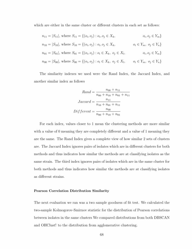
which are either in the same cluster or different clusters in each set as follows:
n11 = |S11|, where S11 = {(oi, oj) : oi, oj ∈ Xk, oi, oj ∈ Ym}
n10 = |S10|, where S10 = {(oi, oj) : oi, oj ∈ Xk, oi ∈ Ym, oj ∈ Yn}
n01 = |S01|, where S01 = {(oi, oj) : oi ∈ Xk, oj ∈ Xl, oi, oj ∈ Ym}
n00 = |S00|, where S00 = {(oi, oj) : oi ∈ Xk, oj ∈ Xl, oi ∈ Ym, oj ∈ Yn}
The similarity indexes we used were the Rand Index, the Jaccard Index, and
another similar index as follows
Rand =n00 + n11
n00 + n10 + n01 + n11
Jaccard =n11
n10 + n01 + n11
Different =n00
n00 + n10 + n01
For each index, values closer to 1 mean the clustering methods are more similar
with a value of 0 meaning they are completely different and a value of 1 meaning they
are the same. The Rand Index gives a complete view of how similar 2 sets of clusters
are. The Jaccard Index ignores pairs of isolates which are in different clusters for both
methods and thus indicates how similar the methods are at classifying isolates as the
same strain. The third index ignores pairs of isolates which are in the same cluster for
both methods and thus indicates how similar the methods are at classifying isolates
as different strains.
Pearson Correlation Distribution Similarity
The next evaluation we ran was a two sample goodness of fit test. We calculated the
two-sample Kolmogorov-Smirnov statistic for the distribution of Pearson correlations
between isolates in the same clusters We compared distributions from both DBSCAN
and OHClust! to the distribution from agglomerative clustering.
68

This test was similar to two-sample goodness of fit test for similarity used in
Section 5.1.2, except instead of comparing the distribution from a single clustering
method to an expected distribution, it compares two sets of clusters against each
other. We ran the test for each of the clustering methods under comparison using the
two-sample Kolmogorov-Smirnov statistic.
Because there isn’t an accepted way of mapping clusters from two different sets of
clusters, we couldn’t test if a single cluster from one clustering method had a similar
distribution to a single cluster from the other clustering method. Instead, we tried to
assess the overall quality of the clusters by using the same Pearson correlation sample
used in the goodness of fit test described in Section 5.1.2. Again, every test was run
separately for each DNA region.
5.2 Isolate Sets
The sets of isolates used for each clustering method were not exactly the same. We
used Montana’s implementation of OHClust! and Agglomerative clustering, which
uses a different method for querying isolates from CPLOP then the implementation
of DBSCAN presented with this thesis. OHClust! and Agglomerative clustering
were run on a set of isolates which included 230 isolates that the isolate set used for
DBSCAN did not have.
The query we used, shown in Figure 4.1, gets the most recent pyroprint which has
not been marked as erroneous from each ITS region for each isolate. After the query,
we filter out isolates which do not have pyroprints for both ITS regions. The query
Montana used also filters isolates without pyroprints for both ITS regions, however
it does not filter pyroprints which are marked as erroneous.
For the most part, both queries get the same isolates. However for some isolates,
all of the pyroprints for an ITS region are marked as erroneous. In this case, the
69
implementation we provide will not return that isolate, but Montana’s implementation
will return it. All but 29 of the extra isolates were because of this difference in queries.
The 201 isolates clustered with erroneous pyroprints likely wont affect the clusters.
Because of their erroneous nature, those isolates likely won’t match anything enough
to be added to any clusters and thus would be noise.
Of the 29 extra isolates which have pyroprints for both ITS regions not marked as
erroneous, 26 of them didn’t actually have any data in the pyroprints, just metadata.
We aren’t certain how they were compared to other isolates, but we assume that it
would default to a Pearson correlation of 0, and thus not be added to any clusters.
After removing those 230 isolates from the clusters produced by OHClust! and
Agglomerative clustering, the two sets still have 6093 isolates in common, so we
consider differences caused by clustering with extra isolates to be negligible.
5.3 Clustering Parameters
This section describes the parameters used for each clustering method which affect
the clusters produced.
5.3.1 DBSCAN
DBSCAN has two parameters: Eps, which is the distance at which two points are
considered neighbors, and MinPts, which is the minimum number of neighbors a
point must have before they are all considered a cluster. For our purpose, we actually
need two Eps parameters, one for each region. We used the α Pearson Correlation
threshold of 0.995 for Eps for both regions because it is a semantic value meaning
that the two isolates are definitely similar. Technically, we used distances to cluster
thus the thresholds we used were the converted values found in Table 3.1.
70

For MinPts, we tried two values, 1 and 3, for all of the tests. For the purpose
of evaluation, we consider these two separate clustering methods denoted DBSCAN 1
and DBSCAN 3. With a MinPts value of 1, DBSCAN produces the same clusters as
minimum/single-link Agglomerative clustering (not to be confused with average-link
Agglomerative clustering which is the method currently used by the research group).
A value of 2 also produces the same clusters except that the minimum cluster size
is 3 as opposed to 2. At MinPts = 3, DBSCAN starts producing ”density-based”
clusters, and as such, is the second value we chose to evaluate.
5.3.2 Agglomerative Clustering and OHClust!
Agglomerative Clustering doesn’t technically need parameters, but since it produces
a dendrogram, in order to get clusters we need to pick a cutoff value for cluster
similarity. We used the β Pearson Correlation threshold of 0.99 for the cutoff of the
average pairwise Pearson correlation between points of two clusters
OHClust! is based on Agglomerative clustering and thus needs a cutoff value as
well. We used the same cutoff of 0.99 for OHClust!. In addition, OHClust! uses an
ontology to guide the order of comparisons. The ontology definition we used is shown
in Figure 5.1.
5.4 Clusters Statistics
We start by providing descriptive statistics on the number and sizes of the clusters
produced by each method. Table 5.1 shows the number of isolates which were not
clustered (noise), the number of clusters, and statistics about the size of the clusters
produced by each method. The DBSCAN methods leave the most isolates unclus-
tered and have fewer number of clusters than the average-link Agglomerative-based
methods. The DBSCAN methods have larger maximum cluster size and mean cluster
71
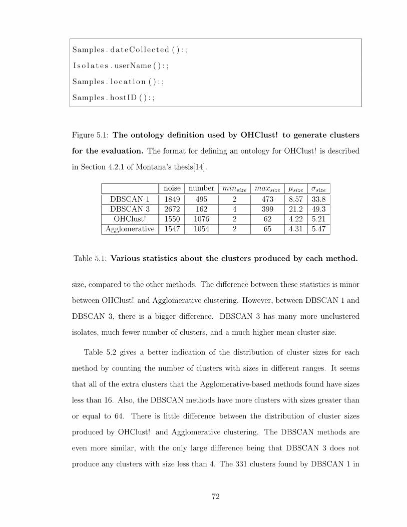
Samples . da t eCo l l e c t ed ( ) : ;
I s o l a t e s . userName ( ) : ;
Samples . l o c a t i o n ( ) : ;
Samples . hostID ( ) : ;
Figure 5.1: The ontology definition used by OHClust! to generate clusters
for the evaluation. The format for defining an ontology for OHClust! is described
in Section 4.2.1 of Montana’s thesis[14].
noise number minsize maxsize µsize σsize
DBSCAN 1 1849 495 2 473 8.57 33.8DBSCAN 3 2672 162 4 399 21.2 49.3OHClust! 1550 1076 2 62 4.22 5.21
Agglomerative 1547 1054 2 65 4.31 5.47
Table 5.1: Various statistics about the clusters produced by each method.
size, compared to the other methods. The difference between these statistics is minor
between OHClust! and Agglomerative clustering. However, between DBSCAN 1 and
DBSCAN 3, there is a bigger difference. DBSCAN 3 has many more unclustered
isolates, much fewer number of clusters, and a much higher mean cluster size.
Table 5.2 gives a better indication of the distribution of cluster sizes for each
method by counting the number of clusters with sizes in different ranges. It seems
that all of the extra clusters that the Agglomerative-based methods found have sizes
less than 16. Also, the DBSCAN methods have more clusters with sizes greater than
or equal to 64. There is little difference between the distribution of cluster sizes
produced by OHClust! and Agglomerative clustering. The DBSCAN methods are
even more similar, with the only large difference being that DBSCAN 3 does not
produce any clusters with size less than 4. The 331 clusters found by DBSCAN 1 in
72

[2, 4) [4, 8) [8, 16) [16, 32) [32, 64) [64, 128) [128,∞)
DBSCAN 1 331 90 38 17 10 4 5DBSCAN 3 0 86 38 18 10 5 5OHClust! 693 282 78 12 11 0 0
Agglomerative 668 279 82 15 9 1 0
Table 5.2: Distribution of cluster sizes for each clustering method.
this range account for almost all of the diffence in total number of clusters between
DBSCAN 1 and DBSCAN 3.
An additional factor to consider is that, unlike Agglomerative clustering, density-
based clustering has the possibility of clustering one isolate in multiple clusters. This
can only occur for border points because if a point with enough neighbors to be
considered a core point is found between two clusters, then clusters will combine
into one. With a MinPts value of 1, all points are either noise or core points thus
there cannot be points in multiple clusters. DBSCAN 3 however, clustered 9 isolates
in multiple clusters for the full dataset. This is a small enough number that we
don’t think it will have a noticeable effect on the results. It is unclear what the
interpretation of an isolate in multiple clusters would be when clusters are considered
strains for our use case. It could suggest that the two strains should be combined into
a single strain. Alternatively, the fact that it is possible could mean density-based
clustering is not a good match for identifying strains in pyroprinted isolates.
5.5 Evaluation Results
This section presents the results from each of the evaluations we ran and gives an
analysis of these results. The evaluations are described in Section 5.1
73
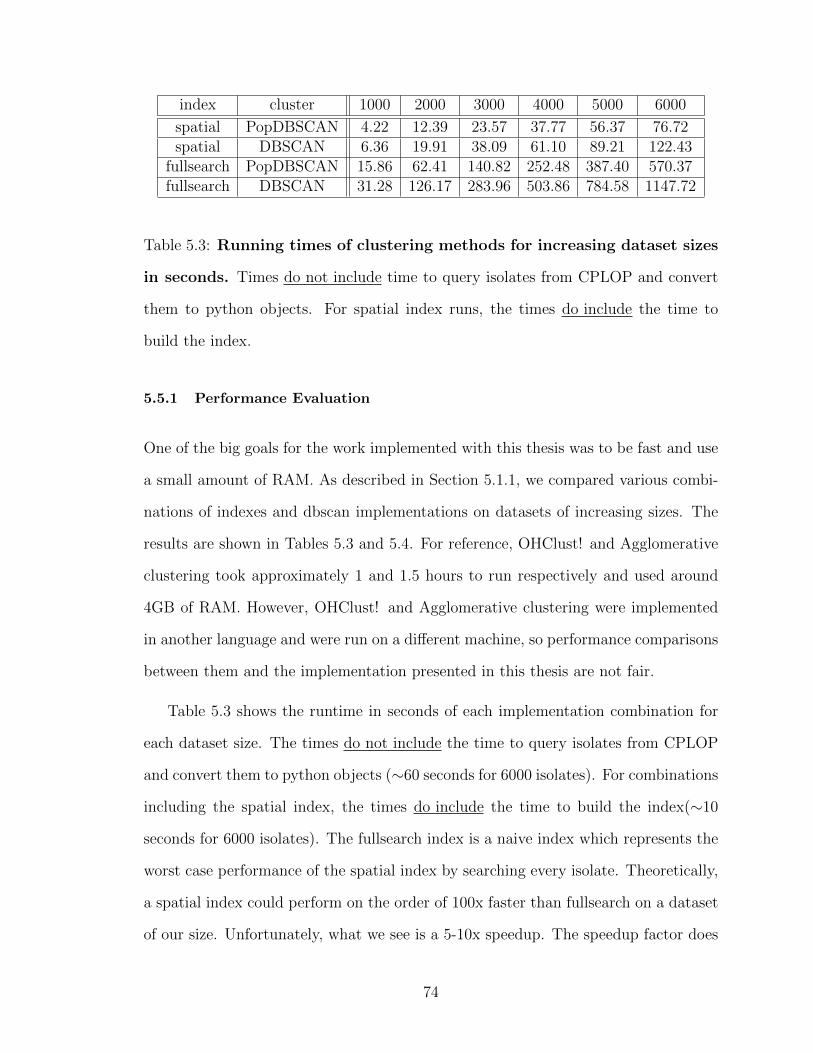
index cluster 1000 2000 3000 4000 5000 6000
spatial PopDBSCAN 4.22 12.39 23.57 37.77 56.37 76.72spatial DBSCAN 6.36 19.91 38.09 61.10 89.21 122.43
fullsearch PopDBSCAN 15.86 62.41 140.82 252.48 387.40 570.37fullsearch DBSCAN 31.28 126.17 283.96 503.86 784.58 1147.72
Table 5.3: Running times of clustering methods for increasing dataset sizes
in seconds. Times do not include time to query isolates from CPLOP and convert
them to python objects. For spatial index runs, the times do include the time to
build the index.
5.5.1 Performance Evaluation
One of the big goals for the work implemented with this thesis was to be fast and use
a small amount of RAM. As described in Section 5.1.1, we compared various combi-
nations of indexes and dbscan implementations on datasets of increasing sizes. The
results are shown in Tables 5.3 and 5.4. For reference, OHClust! and Agglomerative
clustering took approximately 1 and 1.5 hours to run respectively and used around
4GB of RAM. However, OHClust! and Agglomerative clustering were implemented
in another language and were run on a different machine, so performance comparisons
between them and the implementation presented in this thesis are not fair.
Table 5.3 shows the runtime in seconds of each implementation combination for
each dataset size. The times do not include the time to query isolates from CPLOP
and convert them to python objects (∼60 seconds for 6000 isolates). For combinations
including the spatial index, the times do include the time to build the index(∼10
seconds for 6000 isolates). The fullsearch index is a naive index which represents the
worst case performance of the spatial index by searching every isolate. Theoretically,
a spatial index could perform on the order of 100x faster than fullsearch on a dataset
of our size. Unfortunately, what we see is a 5-10x speedup. The speedup factor does
74

index cluster 1000 2000 3000 4000 5000 6000
spatial popdbscan 30.1 35.5 40.2 46.0 50.5 55.8spatial dbscan 29.7 35.6 40.2 45.8 50.8 58.2
fullsearch popdbscan 28.9 33.8 38.9 43.9 49.1 54.6fullsearch dbscan 29.0 33.9 38.8 43.5 48.7 53.6
Table 5.4: RAM usage of clustering methods for increasing dataset sizes in
MB.
increase as the the database grows, so we did achieve an implementation that scales
better with a growing database. However there is certainly room for improvement.
We implemented the DBSCAN method based on the original DBSCAN algorithm[9]
as shown in Figures 2.5 and 2.6. PopDBSCAN is an implementation of the modified
algorithm we designed for this thesis. The results show a consistent 2x speedup of
PopDBSCAN over DBSCAN for when using the fullsearch index, and a consistent
1.5x speedup when using the spatial index. It is possible that with better balancing
after deletion, a different spatial index could see higher speedups.
Table 5.4 shows the maximum RAM usage of each implementation combination for
each dataset size. The results show that the fullsearch index consistently uses around
2MB less than the spatial index. The results show little difference in RAM usage
between PopDBSCAN and DBSCAN. For every implementation combination, there
seems to be a consistent difference of around 5MB between results from increasing
dataset sizes, implying that the RAM usage scales linearly with the dataset size.
Most importantly, the RAM usage for our current dataset size of ∼6000 is far below
the 3GB of RAM available on CPLOP’s server, which also needs to run MySQL and
Apache web server.
75
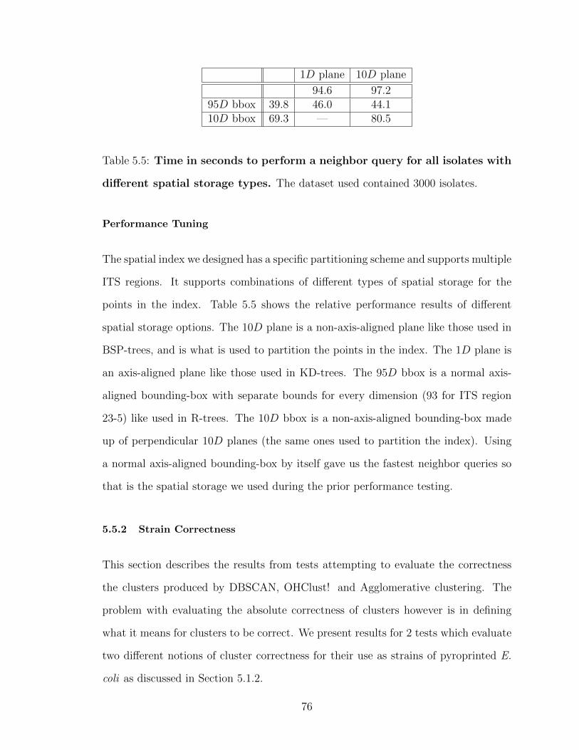
1D plane 10D plane
94.6 97.295D bbox 39.8 46.0 44.110D bbox 69.3 — 80.5
Table 5.5: Time in seconds to perform a neighbor query for all isolates with
different spatial storage types. The dataset used contained 3000 isolates.
Performance Tuning
The spatial index we designed has a specific partitioning scheme and supports multiple
ITS regions. It supports combinations of different types of spatial storage for the
points in the index. Table 5.5 shows the relative performance results of different
spatial storage options. The 10D plane is a non-axis-aligned plane like those used in
BSP-trees, and is what is used to partition the points in the index. The 1D plane is
an axis-aligned plane like those used in KD-trees. The 95D bbox is a normal axis-
aligned bounding-box with separate bounds for every dimension (93 for ITS region
23-5) like used in R-trees. The 10D bbox is a non-axis-aligned bounding-box made
up of perpendicular 10D planes (the same ones used to partition the index). Using
a normal axis-aligned bounding-box by itself gave us the fastest neighbor queries so
that is the spatial storage we used during the prior performance testing.
5.5.2 Strain Correctness
This section describes the results from tests attempting to evaluate the correctness
the clusters produced by DBSCAN, OHClust! and Agglomerative clustering. The
problem with evaluating the absolute correctness of clusters however is in defining
what it means for clusters to be correct. We present results for 2 tests which evaluate
two different notions of cluster correctness for their use as strains of pyroprinted E.
coli as discussed in Section 5.1.2.
76
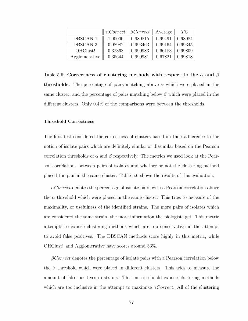
αCorrect βCorrect Average TC
DBSCAN 1 1.00000 0.989815 0.99491 0.98984DBSCAN 3 0.98982 0.993463 0.99164 0.99345OHClust! 0.32368 0.999983 0.66183 0.99809
Agglomerative 0.35644 0.999981 0.67821 0.99818
Table 5.6: Correctness of clustering methods with respect to the α and β
thresholds. The percentage of pairs matching above α which were placed in the
same cluster, and the percentage of pairs matching below β which were placed in the
different clusters. Only 0.4% of the comparisons were between the thresholds.
Threshold Correctness
The first test considered the correctness of clusters based on their adherence to the
notion of isolate pairs which are definitely similar or dissimilar based on the Pearson
correlation thresholds of α and β respectively. The metrics we used look at the Pear-
son correlations between pairs of isolates and whether or not the clustering method
placed the pair in the same cluster. Table 5.6 shows the results of this evaluation.
αCorrect denotes the percentage of isolate pairs with a Pearson correlation above
the α threshold which were placed in the same cluster. This tries to measure of the
maximality, or usefulness of the identified strains. The more pairs of isolates which
are considered the same strain, the more information the biologists get. This metric
attempts to expose clustering methods which are too conservative in the attempt
to avoid false positives. The DBSCAN methods score highly in this metric, while
OHClust! and Agglomerative have scores around 33%.
βCorrect denotes the percentage of isolate pairs with a Pearson correlation below
the β threshold which were placed in different clusters. This tries to measure the
amount of false positives in strains. This metric should expose clustering methods
which are too inclusive in the attempt to maximize αCorrect. All of the clustering
77

methods scored high on this, although OHClust! and Agglomerative clustering scored
higher.
Threshold correctness, denoted TC, combines αCorrect and βCorrect weighted
based on the number of isolate pairs with corresponding Pearson correlations. Because
the majority of isolate pairs in the dataset have a pearson correlation below β, the
TC is highly biased and very similar to βCorrect.
As an unbiased alternative to the TC score, we also calculated the average of
αCorrect and βCorrect. The relative usefulness of each score in determining the
correctness of the strains depends on the research group’s value of strain maximal-
ity/usefulness vs a low chance of false positives. The absolute usefulness of these
scores depends on the research group’s confidence in the α and β thresholds.
Pearson Correlation Distribution Correctness
The second test we performed for cluster correctness was a two-sample Kolmogorov-
Smirnov goodness of fit test. As described in Section 5.1.2, we performed a two-sample
Kolmogorov-Smirnov goodness of fit test. This tests whether two samples came from
the same distribution. We used pairwise Pearson Correlations from isolates within
the same clusters as samples for each clustering method. Then we used to goodness
of fit test to see if the methods produce clusters with the same Pearson correlation
distribution as the expected distribution. The results of these tests are shown in
Table 5.7.
The Kolmogorov-Smirnov test computes a statistic, denoted KSstat. This statistic
is then converted to a pValue, or the probability of a false negative, i.e rejecting the
null hypothesis that two samples were drawn from the same distribution when in fact
they were. The results show that none of the methods have more than a remote chance
of matching the expected distribution. The probabilities are so small that relative
78
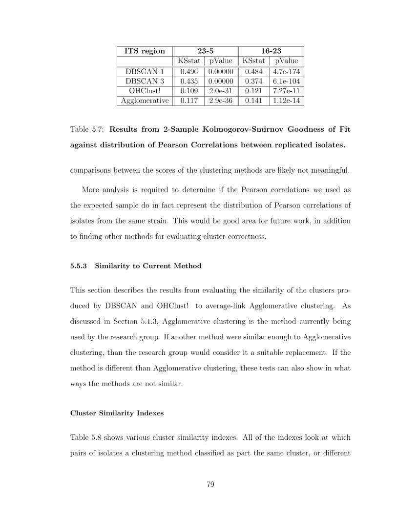
ITS region 23-5 16-23KSstat pValue KSstat pValue
DBSCAN 1 0.496 0.00000 0.484 4.7e-174DBSCAN 3 0.435 0.00000 0.374 6.1e-104OHClust! 0.109 2.0e-31 0.121 7.27e-11
Agglomerative 0.117 2.9e-36 0.141 1.12e-14
Table 5.7: Results from 2-Sample Kolmogorov-Smirnov Goodness of Fit
against distribution of Pearson Correlations between replicated isolates.
comparisons between the scores of the clustering methods are likely not meaningful.
More analysis is required to determine if the Pearson correlations we used as
the expected sample do in fact represent the distribution of Pearson correlations of
isolates from the same strain. This would be good area for future work, in addition
to finding other methods for evaluating cluster correctness.
5.5.3 Similarity to Current Method
This section describes the results from evaluating the similarity of the clusters pro-
duced by DBSCAN and OHClust! to average-link Agglomerative clustering. As
discussed in Section 5.1.3, Agglomerative clustering is the method currently being
used by the research group. If another method were similar enough to Agglomerative
clustering, than the research group would consider it a suitable replacement. If the
method is different than Agglomerative clustering, these tests can also show in what
ways the methods are not similar.
Cluster Similarity Indexes
Table 5.8 shows various cluster similarity indexes. All of the indexes look at which
pairs of isolates a clustering method classified as part the same cluster, or different
79
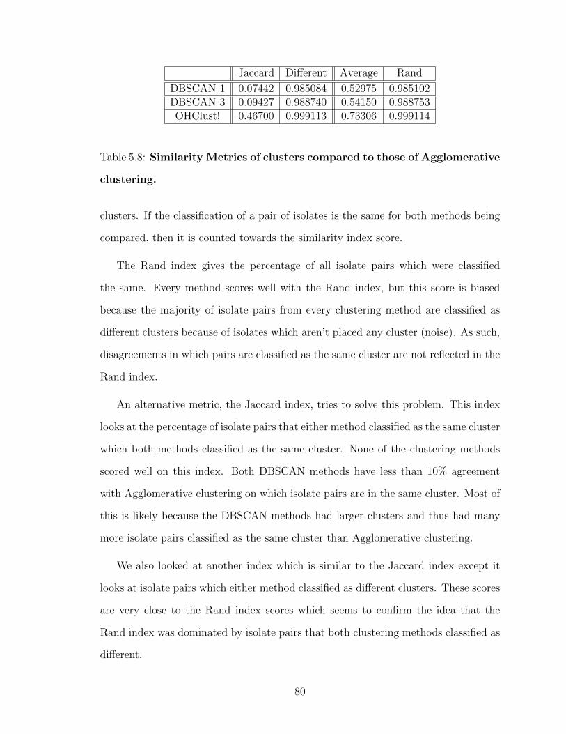
Jaccard Different Average Rand
DBSCAN 1 0.07442 0.985084 0.52975 0.985102DBSCAN 3 0.09427 0.988740 0.54150 0.988753OHClust! 0.46700 0.999113 0.73306 0.999114
Table 5.8: Similarity Metrics of clusters compared to those of Agglomerative
clustering.
clusters. If the classification of a pair of isolates is the same for both methods being
compared, then it is counted towards the similarity index score.
The Rand index gives the percentage of all isolate pairs which were classified
the same. Every method scores well with the Rand index, but this score is biased
because the majority of isolate pairs from every clustering method are classified as
different clusters because of isolates which aren’t placed any cluster (noise). As such,
disagreements in which pairs are classified as the same cluster are not reflected in the
Rand index.
An alternative metric, the Jaccard index, tries to solve this problem. This index
looks at the percentage of isolate pairs that either method classified as the same cluster
which both methods classified as the same cluster. None of the clustering methods
scored well on this index. Both DBSCAN methods have less than 10% agreement
with Agglomerative clustering on which isolate pairs are in the same cluster. Most of
this is likely because the DBSCAN methods had larger clusters and thus had many
more isolate pairs classified as the same cluster than Agglomerative clustering.
We also looked at another index which is similar to the Jaccard index except it
looks at isolate pairs which either method classified as different clusters. These scores
are very close to the Rand index scores which seems to confirm the idea that the
Rand index was dominated by isolate pairs that both clustering methods classified as
different.
80
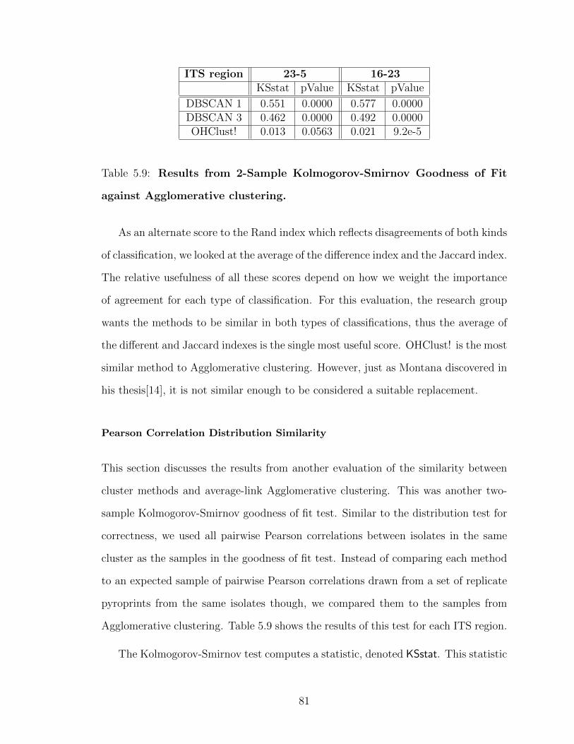
ITS region 23-5 16-23KSstat pValue KSstat pValue
DBSCAN 1 0.551 0.0000 0.577 0.0000DBSCAN 3 0.462 0.0000 0.492 0.0000OHClust! 0.013 0.0563 0.021 9.2e-5
Table 5.9: Results from 2-Sample Kolmogorov-Smirnov Goodness of Fit
against Agglomerative clustering.
As an alternate score to the Rand index which reflects disagreements of both kinds
of classification, we looked at the average of the difference index and the Jaccard index.
The relative usefulness of all these scores depend on how we weight the importance
of agreement for each type of classification. For this evaluation, the research group
wants the methods to be similar in both types of classifications, thus the average of
the different and Jaccard indexes is the single most useful score. OHClust! is the most
similar method to Agglomerative clustering. However, just as Montana discovered in
his thesis[14], it is not similar enough to be considered a suitable replacement.
Pearson Correlation Distribution Similarity
This section discusses the results from another evaluation of the similarity between
cluster methods and average-link Agglomerative clustering. This was another two-
sample Kolmogorov-Smirnov goodness of fit test. Similar to the distribution test for
correctness, we used all pairwise Pearson correlations between isolates in the same
cluster as the samples in the goodness of fit test. Instead of comparing each method
to an expected sample of pairwise Pearson correlations drawn from a set of replicate
pyroprints from the same isolates though, we compared them to the samples from
Agglomerative clustering. Table 5.9 shows the results of this test for each ITS region.
The Kolmogorov-Smirnov test computes a statistic, denoted KSstat. This statistic
81
is then converted to a pValue, or the probability of a false negative, i.e rejecting the
null hypothesis that two samples were drawn from the same distribution when in fact
they were. The results show that the DBSCAN methods produce clusters with a
different distribution than Agglomerative clustering with practically no chance of a
false negative for both ITS regions. OHClust! on the other hand, while it rejects the
null hypothesis for the 16-23 region, it cannot reject the null hypothesis for the 23-5
region with a confidence of 95%. Unfortunately, the research team would need it to
fail to reject for both ITS regions in order to consider the methods similar.
82
CHAPTER 6
CONCLUSION
The work described in this thesis provides the Cal Poly Library Of Pyroprints (CPOLP)
research group with an alternative method of strain identification. Identifying strains
speeds up Microbial Source Tracking comparisons and allows researchers to perform
longitudinal and transference studies.
The contributions of this thesis are the following:
• A modified DBSCAN algorithm: We presented a clustering method based
on DBSCAN which allows for the removal of points from the search space after
they have been seen once. For the CPLOP dataset, This modification results
in up to a 2x speedup over the original DBSCAN algorithm.
• A faster method for comparing pyroprints: This thesis presented a new
method for comparing pyroprints, Euclidean distance of Z-Scores. This new
method is algebraically related to Pearson correlation (the current method),
allowing reuse of previous statistical analysis. We precomputed Z-Score values
for every pyroprint which speeds up comparisons with both the current method
and the new method. We showed that we can store pyroprint Z-Scores in a
spatial index to speed up clustering.
• A spatial index that works with E. coli pyroprints: This thesis pre-
sented a spatial index tailored for the characteristics of the CPLOP dataset.
It supports dense, high-dimensional data by partitioning the search space with
multidimensional planes and storing bounding volumes for subgroups of data.
The index also supports multiple regions for each data point with separate
search radii.
83
• Better evaluation metrics of clusters for CPLOP: Finally, this thesis
contributed methods for evaluating the correctness of identified strains. We ran
these methods on clusters generated by this work as well as those generated by
previous clustering methods OHClust! and Agglomerative clustering. We were
able to characterize some of the differences between all of the clustering methods
that have been tried to this date for identifying strains of E. coli pyroprints.
6.1 Future Work
There are many avenues of future work. First, defining strains in CPLOP is still
an open problem. Next, researchers could try to improve the performance of our
design/implementation. Another option would be to try clustering in a way that
creates extra information for the biologists to analyse. Other work could try to
provide alternatives to this work that are more correct. Finally, researchers could
look into other applications for the algorithms developed for this thesis.
6.1.1 E. coli Strains
The research group wants to answer the question: which clustering method gives the
best definition of a strain for pyroprinted E. coli? This thesis attempted to answer
part of the question by evaluating if density-based clusters are a suitable replacement
for the current clustering method. Answering this question will require more analysis
of the results presented in this thesis, and may also require further testing.
The research group also wants to determine the usefulness of identified strains for
MST. Future work could look at the purity of strains, the amount of agreement on
host species between isolates in the same strains. If a strain has been seen in many
different host species, then researchers won’t have a way to know which of those host
84
species an unknown isolate matching that strain came from, and the strain would not
be useful for MST.
6.1.2 Performance
The first area for future work is improving the performance of the algorithms pre-
sented in this thesis. This is the area that we have the most ideas for, and because
of the genericy of our implementation, many of them would be easy to try.
One option would be to try persisting data and try incremental clustering. We are
already persisting the clusters in CPLOP, so we are partway there, but the limiting
factor to clustering is the neighbor lookups. Researchers could look into persisting
the spatial index or even persisting a map of isolates to their neighbors. Our current
tree construction algorithm runs fairly fast and it’s the querying that takes most of
the runtime. Researchers could also try caching all pairwise distance computations
between pyroprints, however since this would not all fit in RAM on our current server,
they would need to keep most of it in disk and load it dynamically which could offset
the benefits of precomputing. Another option would be to try using another clustering
algorithm like incDBSCAN which performs less neighbor lookups in the first place,
given some previously discovered clusters.
Other ideas to try would be using different filtering methods for determining if the
isolates in a subtree possibly match a neighbor query. This would include trying using
only the split plane at higher levels in the tree and only the bounding box in lower
levels of the tree. Or researchers could try having some nodes only filter on a single
region, perhaps alternating between regions on successive levels. Finally, they could
of course try different filtering methods such as bounding spheres. Our spatial index
implementation is generic enough to support all of these possibilities. The neighbor
query will work unmodified; all that the researchers need to do is implement any new
85
filters and modify the construction of the index to add whichever filters they want to
each node in the tree.
Another idea to look as is using different partitioning methods to construct the
spatial index. The tree implementation is generic in how many children are at each
level and the information on how the parent was split is encoded in the children
themselves, so it should support many different partitioning schemes.
An idea that the implementation does not generically support is rebalancing the
tree after points are removed. Currently empty nodes are removed from the tree and
bounding volumes updated to fit the data of only the remaining points, which would
be fine if the queries were balanced. However the query pattern of DBSCAN will
query points near each other one after another and when points are removed in this
fashion, it will result in a lopsided tree. The solution would be to repartition the
points every once in a while, perhaps more often in subtrees.
Finally, the implementation itself has lots of room for improvement from a per-
formance aspect. The current implementation introduces lots of overhead in the tree
traversal, some of which could be better implemented. An example would be using
array indexing instead of hashmap lookups for getting the pyroprint from a particular
region. However, traversal is currently a small part of the runtime which is domi-
nated by pyroprint and filter comparisons. The library we used for these comparisons
is highly optimized, but perhaps there are faster libraries out there for our purposes.
In addition, rewriting the codebase in a faster language could also help.
6.1.3 Additional Analysis Opportunities
Another avenue of future work would be to provide more information for the biologists
to analyze. Strains give the biologists a lot of opportunities for analysis because they
can look for patterns between isolates in the same strain. We have some ideas for
86

finding other relationships between isolates, which the biologists might be interested
in.
The first idea is to cluster isolates twice, once for each region. Isolates that were
in the same cluster for both regions will also be is the same strain. This design would
allow the biologists to look for patterns within isolates that are indistinguishable in
one ITS region but not the other, implying some relationship but not as strongly as
the full strain. Additionally, it finds relationships between pairs of strains where their
isolates match in one of the ITS regions.
A hierarchical clustering algorithm would provide new information for strain anal-
ysis. It could be used to look for strains that are close to each other, or to look for
subgroups within a strain. Additionally it could be used to see if different strains have
different amounts of spread. Perhaps some clusters are formed at higher thresholds
while others would form if the threshold was just a little bit more lax.
6.1.4 Correctness
Another avenue of future research is in trying to find a method the produces clusters
that better match the Biologist’s notion of strains for pyroprints.
First of all, a method of evaluating the correctness of clusters is needed. This
paper presented two possible methods, but more analysis is needed to determine how
well those methods are at determining strain correctness. Testing other correctness
measures could also be useful.
One option is the same idea that inspired this thesis. There are other cluster-
ing methods which have not yet been tried with pyroprints and evaluated on their
similarity to the Biologist’s notion of strains. A method that would likely do very
well on our pairwise Pearson correlation distribution evaluation is distribution-based
clustering.
87
Another idea to consider is slightly changing what is considered correct by trying
out different metrics for comparing isolates/pyroprints. Perhaps there are other ways
to normalize the pyroprints that better account for the noise in the pyroprinting
process. An example of a different but similar normalization would be to normalize
the pyroprint by the mean and standard deviation of the first ∼10 dispensations
which sequence conserved DNA (so every isolate and every locus will have the same
DNA), instead of the mean and standard deviation of every dispensation.
6.1.5 Applications
The last avenue of future research would be to determine how well the algorithms
presented in this thesis apply to other applications.
The modified DBSCAN algorithm should easily work for normal DBSCAN ap-
plications. All it needs is a spatial index with the ability to quickly remove points.
A limitation of the modified DBSCAN algorithm though is that if there are lots of
noise in the dataset and most of the points would be part of the same cluster if
minPts = 1, then the performance could degrade to O(N2) even with a O(N logN)
neighbor lookup.
Other applications for the spatial index developed for this thesis are less obvious.
The multi-region aspect of the index was designed for the unique problem of spatially
indexing pyroprints from the same isolate. The design works with a single region
though in which case the index is basically a hybrid Binary Space Partitioning tree
and Bounding Volume Hierarchy. This could potentially be applicable to many of the
same uses as other spatial indexes, especially those with high-dimensional data.
88

BIBLIOGRAPHY
[1] Mihael Ankerst, Markus M Breunig, Hans-Peter Kriegel, and Jorg Sander.
Optics: Ordering points to identify the clustering structure. ACM
Sigmod Record, 28(2):49–60, 1999.
[2] Norbert Beckmann, Hans-Peter Kriegel, Ralf Schneider, and Bernhard
Seeger. The r*-tree: an efficient and robust access method for points
and rectangles. ACM SIGMOD Record, 19(2):322–331, 1990.
[3] Jon Louis Bentley. Multidimensional binary search trees used for associative
searching. Communications of the ACM, 18(9):509–517, 1975.
[4] Stefan Berchtold, Daniel A Keim, and Hans-Peter Kriegel. The x-tree: An
index structure for high-dimensional data. Readings in multimedia
computing and networking, 451, 2001.
[5] Michael W Black, Jennifer VanderKelen, Aldrin Montana, Alexander Dekht-
yar, Emily Neal, Anya Goodman, and Christopher L Kitts. Pyroprint-
ing: A rapid and flexible genotypic fingerprinting method for typ-
ing bacterial strains. Journal of microbiological methods, 105:121–129,
2014.
[6] Kaushik Chakrabarti and Sharad Mehrotra. The hybrid tree: An index
structure for high dimensional feature spaces. In Data Engineering,
1999. Proceedings., 15th International Conference on, pages 440–447.
IEEE, 1999.
[7] J. Dillard, J. Kent, D. Britton, T. Branck, A. Frey, P. McCreesh, J. Van-
derKelen, C. Kitts, and M. Black. E. coli strain demographics and
transmission in cattle, Jan 2013.
89
[8] Martin Ester, Hans-Peter Kriegel, Jorg Sander, Michael Wimmer, and Xi-
aowei Xu. Incremental clustering for mining in a data warehousing
environment. In VLDB, volume 98, pages 323–333. Citeseer, 1998.
[9] Martin Ester, Hans-Peter Kriegel, Jorg Sander, and Xiaowei Xu. A density-
based algorithm for discovering clusters in large spatial databases with
noise. In Kdd, volume 96, pages 226–231, 1996.
[10] Antonin Guttman. R-trees: a dynamic index structure for spatial search-
ing. ACM Sigmod Record, 14(2):47–57, 1984.
[11] Norio Katayama and Shin’ichi Satoh. The sr-tree: An index structure for
high-dimensional nearest neighbor queries. ACM SIGMOD Record,
26(2):369–380, 1997.
[12] King-Ip Lin, Hosagrahar V Jagadish, and Christos Faloutsos. The tv-tree:
An index structure for high-dimensional data. The VLDB Journal,
3(4):517–542, 1994.
[13] Jeffrey D. McGovern, Alexander Dekhtyar, Chris Kitts, Jennifer VanderKe-
len Michael Black, and Anya Goodman. Leveraging the k-nearest
neighbors classification algorithm for microbial source tracking using
a bacterial dna fingerprint library. In Proceedings of the Second Work-
shop on Semantic Data Analytics and Bioinformatics (SDAB 2015),
Washington, DC, Nov 2015.
[14] Aldrin Montana. Algorithms for library-based microbial source track-
ing. Master’s thesis, California Polytechnic State University, San Luis
Obispo, California, 2013.
[15] Emily R Neal. Escherichia coli strain diversity in humans: effects of sam-
pling effort and methodology. Master’s thesis, California Polytechnic
State University, San Luis Obispo, 2013.
90
[16] M Patella, P Ciaccia, and P Zezula. M-tree: An efficient access method
for similarity search in metric spaces. In Proc. of the International
Conference on Very Large Databases (VLDB). Athens, Greece, pages
1241–1253, 1997.
[17] Troy M Scott, Joan B Rose, Tracie M Jenkins, Samuel R Farrah, and
Jerzy Lukasik. Microbial source tracking: current methodology and fu-
ture directions. Applied and Environmental Microbiology, 68(12):5796–
5803, 2002.
[18] Diana Shealy. Exploration of pyroprinting for environmental forensics.
Technical report, California Polytechnic State University, San Luis
Obispo, California, June 2012.
[19] Joyce M Simpson, Jorge W Santo Domingo, and Donald J Reasoner. Mi-
crobial source tracking: state of the science. Environmental science &
technology, 36(24):5279–5288, 2002.
[20] Jan Lorenz Soliman. Cplop: Cal poly library of pyroprints. Master’s thesis,
California Polytechnic State University, San Luis Obispo, California,
2013.
[21] Wei Wang, Jiong Yang, and Richard Muntz. Pk-tree: a spatial index
structure for high dimensional point data. Information organization
and databases, pages 281–293, 2000.
91


![RECOME: a New Density-Based Clustering Algorithm Using ... · RECOME: a New Density-Based Clustering Algorithm Using Relative KNN Kernel Density Yangli-ao Geng[1] Qingyong Li[1] Rong](https://img.dokumen.tips/doc/110x75/5ae3962f7f8b9ae74a8de79f/recome-a-new-density-based-clustering-algorithm-using-a-new-density-based-clustering.jpg)