IOP PUBLISHING PHYSICS IN MEDICINE AND BIOLOGY

Phys. Med. Biol. 54 (2009) 1435–1456 doi:10.1088/0031-9155/54/6/004

Denoising human cardiac diffusion tensor magneticresonance images using sparse representationcombined with segmentation

L J Bao1, Y M Zhu1,2, W Y Liu1,2, P Croisille2, Z B Pu1, M Robini2

and I E Magnin1

1 HIT—INSA Sino French Research Centre for Biomedical Imaging, Harbin Institute ofTechnology, Harbin, People’s Republic of China2 CREATIS-LRMN, CNRS UMR 5220, Inserm U630, INSA of Lyon, University of Lyon 1,Villeurbanne, France

E-mail: baolij@gmail.com

Received 20 May 2008, in final form 18 January 2009Published 13 February 2009Online at stacks.iop.org/PMB/54/1435

Abstract

Cardiac diffusion tensor magnetic resonance imaging (DT-MRI) is noisesensitive, and the noise can induce numerous systematic errors in subsequentparameter calculations. This paper proposes a sparse representation-basedmethod for denoising cardiac DT-MRI images. The method first generatesa dictionary of multiple bases according to the features of the observedimage. A segmentation algorithm based on nonstationary degree detectoris then introduced to make the selection of atoms in the dictionary adapted tothe image’s features. The denoising is achieved by gradually approximatingthe underlying image using the atoms selected from the generated dictionary.The results on both simulated image and real cardiac DT-MRI images from exvivo human hearts show that the proposed denoising method performs betterthan conventional denoising techniques by preserving image contrast and finestructures.

(Some figures in this article are in colour only in the electronic version)

1. Introduction

Diffusion tensor magnetic resonance imaging (DT-MRI) is at present the only means forin vivo and nondestructive characterization of the three-dimensional (3D) diffusion and fibrearchitecture of human anatomical organs such as brain white matter (Basser et al 1994),skeletal muscle (Galban et al 2005), spinal cord (Schwartz et al 2005) and myocardium(Scollan and Holmes 2000). It is well known that myocardial fibre orientation is altered invarious cardiac diseases such as myocardial infarction, ischaemic heart disease and ventricular

0031-9155/09/061435+22$30.00 © 2009 Institute of Physics and Engineering in Medicine Printed in the UK 1435

1436 L J Bao et al

hypertrophy (Wu and Tseng 2006). Therefore, detailed information about 3D fibre structuresof myocardium can provide important cues to the understanding of the heart’s physiologicaland functional properties, and to the diagnosis of heart diseases. However, cardiac DT-MRI is highly susceptible to noise. The noise, primarily at the level of diffusion-weightedimage (DWI), obeys a Rician distribution (Gudbjartsson and Patz 1995, Macovski 1996).The noise in DT-MRI is the subject of several papers (Basser and Pajevic 2000, Koayet al 2007). The noise in DWIs produces errors in the subsequent calculations of the tensor,eigenvalues, eigenvectors, mean diffusivity (MD), diffusion anisotropy indices (DAIs) andfibre orientations. These errors include, for example, positive bias in fractional anisotropy(FA), negative eigenvalues, disorder of the eigenvectors and tracked fibres. So improving thesignal-to-noise ratio (SNR) is crucial for practical utility of DT-MRI in human hearts, andnoise removal techniques constitute the most efficient way without additional acquisitions.

Numerous denoising algorithms have been proposed for magnetic resonance (MR) imagesin the past decades (Awate and Whitaker 2007, Basu et al 2006, Gerig and Kubler 1992, Gilboaet al 2004, Hamarneh and Hradsky 2007). At present, the widely used denoising methods arebased on the partial-differential-equation (PDE) filter (Perona and Malik 1990) and waveletalgorithm. The PDE filter, also known as the anisotropic or nonlinear diffusion filter, usesdifferent smoothing degrees proportional to local intensity gradient and can preserve imageedges. It has been employed to filter both scalar images (Chen and Edward 2005) and DT-MRIeigenvector fields (Arsigny et al 2006). However, PDE methods can yield good results onlyfor low noise levels. For high noise levels, their denoising performance is unsatisfactorydue to the serious degradation in contrast. Wavelet-based denoising has also been applied toMR images to achieve a general improvement in image quality (Nowak 1999, Wirestam andBibic 2006). Denoising based on the wavelet transform, like the Fourier transform and thediscrete cosine transform, operates on all information in the data: the image to be denoisedis firstly transformed by means of predefined basis functions, and then an inverse transformis performed after thresholding the transform coefficients. In this condition, not only theuseful information but also the noise in the image is involved in the convolution with thebasis functions during the transformation. Moreover, how to determine the threshold is also aproblem that limits the accuracy of the final result.

Recently, sparse representation has appeared as a promising theory for many signal andimage processing problems such as compression, independent component analysis, imageinpainting, regularization and denoising, proposed in Elad and Aharon (2006), Pham andSmeulders (2006) and Starck et al (2005), respectively. Unlike classical approaches, sparserepresentation-based denoising (SPDN) is achieved by selecting underlying information in thedata with the aid of atoms generated from different function bases or database. The selectionof function bases should correspond to the data features. Generally, images in practice areusually highly structured since their pixels exhibit strong dependences, especially when theyare spatially proximate, and these dependences carry important information about the structureof the objects. On the other hand, the noise in the image distributes randomly without anyorganized structure. So even if an image is deteriorated by noise, its structure features can stillbe approximated with suitable atoms.

The performance of SPDN strongly depends on the denoising model and the dictionary.Indeed, the denoising model is a linear programming problem with two constraints:approximation stop criterion and sparsity of the representation coefficients. Based on anestimation of the noise intensity, the approximation stop criterion is set up to controlthe approximation procedure. As for the sparsity constraint, it relies on the property ofthe dictionary, so it is critical to generate appropriate dictionary according to the structuresin the observed image. Considering that a real image often contains various contents, a

Denoising human cardiac diffusion tensor magnetic resonance images 1437

N

atoms: gφ : nonzero entries

=D

SK (K>N)

N

α

+

ζ

K

N

Figure 1. Principle of sparse representation.

dictionary with multiple bases was proposed in Granai and Vandergheynst (2004), which is asalient property of SPDN. Starck et al (2005) applied multiple bases to separate the overlappedtextures from underlying image content by employing each basis to represent the whole imagerespectively. The method requires that every basis in the dictionary should be very selective,or it is prone to causing approximation errors. Also note that it is often inefficient to use onebasis to represent the whole image.

In this paper, we develop the current sparse representation to denoise human cardiacDT-MRI data and to examine its effectiveness in improving the quality of DWI, as well asthe accuracy of fibre orientation computation. We propose a segmentation-guided SPDNmethod based on the use of a segmentation mechanism for guiding the choice of suitablebases in the dictionary, thus making the decomposition process more adaptive and efficient.The segmentation employs the concept of nonstationarity degree (NSD), which is particularlyrobust for dealing with noisy data. The proposed method is evaluated on the simulated heartimage and ten ex vivo human hearts, and compared to the PDE-based method (Catte et al1992) and the wavelet-based method (Pizurica et al 2003).

2. Theory

2.1. Sparse representation

Sparse representation, also referred to as ‘atom decomposition’ or ‘sparse approximation’,evolved from non-redundancy orthogonal transformation. It is aimed at representing a givensignal S ∈ �N by a linear combination of a few atoms φg ∈ �N extracted from a dictionaryD ∈ �N×K of K atoms. The sparsity comes from the fact that only a small number of atomsare used. This corresponds to solving the following optimization problem:

αopt = arg minα∈�K

‖α‖0 subject to S = Dα + ξ, 0 � ξ < S, (1)

where, as illustrated in figure 1, ‖α‖0 stands for the number of nonzero entries inrepresentation coefficient vector α ∈ �K , ξ is the approximation error that, in the idealcase, approximates to zero and D ∈ �N×K is a dictionary of K atoms φg which satisfiesD = {φg ∈ �N | ‖φg‖ = 1, g ∈ K}.

Usually, dictionaries are overcomplete with K〉N . Atoms (represented by columns infigure 1) are the primary elements of a dictionary and their size is the same as that of the signalin solution. In sparse representation, atoms are generated from parameterized basis functionssuch as wavelets, curvelet, ridgelet, contourlet, etc. or adaptive trained database (Aharon et al2006). The atoms generated from the same basis function constitute a basis. A dictionary can

1438 L J Bao et al

include either a single basis or multiple bases that make it possible to better represent complexsignals with different feature structures. The given signal S is approximately represented byS = Dαopt.

Therefore, selecting the optimal linear combination of atoms from a dictionary toapproximate the underlying data is an NP-hard problem (nondeterministic polynomial timehard problem), for which a few algorithms have been proposed: matching pursuit (MP, Mallatand Zhang 1993), basis pursuit (BP, Chen et al 1998) and focal under determined system solver(FOCUSS, Gorodnitsky and Rao 1997). The MP is a greedy pursuit algorithm that selectsthe best suitable atoms sequentially in iteration, while the BP is a global optimal algorithmthat finds the sparse representation atoms by convex optimization based on minimizing the l1

norm of the representation coefficients. The FOCUSS is similar to the BP by minimizing thelP norm of the representation coefficients. However, the BP and FOCUSS algorithms havehigh computational cost and in some case, compromised convergence. So, for computationalsimplicity and robustness, we adopt the MP algorithm in this work.

2.2. Image denoising based on sparse representation

Theoretically, sparse representation of an image is the same as that of a signal except thatit is a dictionary composed of 2D atoms. Generally speaking, image denoising based onsparse representation attempts to extract underlying structures from the observed image byrepresenting it with a proper dictionary, whereas the noise is left and is not represented becauseit exhibits no structure feature. The process of approximation is controlled by a stop criterion,determination of which relies on the noise level of the image, the tolerated approximationerror and the constraint on sparsity.

Let y ∈ �N×N be the observed noisy image of the form

y = x + r, (2)

where x denotes the noise-free image, and r is an additive noise with standard deviation σr .According to the sparse representation, the observed noisy image y can be represented by

a column vector y ∈ �N2as

y = Dαopt + ξ + r, (3)

where dictionary D ∈ �N2×K and αopt ∈ �K with K > N2.Actually, each atom in the dictionary is a 2D data as φg ∈ �N×N ; we order it as vector

φg ∈ �N2in accordance with y ∈ �N2

. If we define η = ξ + r , where the residue η representserrors due to the approximation ξ and the noise r, then (3) can be rewritten as

y = Dαopt + η. (4)

Taking into account the sparsity constraint on the representation coefficient vector, SPDNamounts to solving the following optimization problem:

αopt = arg minα∈�K

‖α‖0 subject to ‖y − Dα‖22 = ‖η‖2

2. (5)

In the ideal case, the energy function, which is the difference between the observed noisyimage and the noise-free image, is expressed as ‖y − x‖2

2 = ‖r‖22 = N2 · σ 2

r . In practice,the noise-free image is unknown. Therefore, accounting for the approximation error ξ , theenergy function between the observed image and the reconstructed image (which should be asclose as possible to the noise-free image) can be expressed as ‖y − Dα‖2

2 = ‖ξ + r‖22. When

0 � ‖ξ‖2 � ‖r‖2, we have ‖η‖22 = C · N2 · σ 2

r , where the constant C � 1 is defined so asto achieve an optimal denoising result. The value of C will be discussed in section 5. Since

Denoising human cardiac diffusion tensor magnetic resonance images 1439

we usually do not have the ground truth of the observed image, σr should be replaced by itsestimation. Therefore, updating this in (5) gives

αopt = arg minα∈�K

‖α‖0 subject to ‖y − Dα‖22 = C · N2 · σ 2

r . (6)

Then, the estimated noise-free image is obtained using

x = Dαopt. (7)

When denoising a large-size image using an overcomplete dictionary D ∈ �N2×K ,K > N2, with the size of the dictionary increasing in order O(N4), this considerably raisesthe computational burden. To cope with this problem, we choose to process the large imageusing a sliding window (as implemented in Guleryuz (2005a), (2005b)). We overlap patchesto reduce blocking artefacts, which contributes to improve the accuracy of the reconstructedimage. If the sliding window size is n × n and its step is s, yN×N contains ((N − n + 1)/s)2

patches of size n × n. For each patch, the coefficient vector αij is obtained by representingpatch yij with dictionary D ∈ �n2×K . In this case, (6) becomes

αoptij = arg min

αij ∈�K‖αij‖0, subject to ‖�ijy − Dαij‖2

2 = C · n2 · σ 2r , (8)

where (i, j) designates the locations of patches and �ij is the operator that extracts patchesfrom the image with yij = �ijy.

Accordingly, the denoised image can be obtained as

x =⎛⎝(N−n+1)/s∑

j=1

(N−n+1)/s∑i=1

� ′ij xij

⎞⎠

⎛⎝(N−n+1)/s∑

j=1

(N−n+1)/s∑i=1

� ′ij�ij

⎞⎠

−1

with xij = Dαoptij , (9)

where xij ∈ �n×n corresponds to the denoised version of each patch, x ∈ �N×N to the finaldenoised version of the observed image and � ′

ij to the inverse operation of �ij .Hence, the image denoising model based on SPDN can be rewritten as

{αopt, x} = arg min{αij ∈�K,x}

∑ij

‖αij‖0 + λ∑ij

‖�ijy − Dαij‖22 + γ ‖y − x‖2

2, (10)

where the parameters λ and γ are penalty factors. The denoising model is expressed asa constrained optimization problem with Lagrange multiplier updating the constraint intopenalty terms. It is based on maximum a posteriori estimation. This optimization solutionmeans that to find the sparse approximation of the noise-free image through blocking theobserved image into patches, every restored patch should obey ‖xij − yij‖2

2 � C · n2 · σ 2r . At

the same time, the final reconstructed denoised image satisfies ‖x − y‖22 � C · N2 · σ 2

r . Wecan solve this model using the matching pursuit algorithm described in the next subsection.

2.3. Approximation with matching pursuit

The approximation of xij in the subsection 2.2 can be calculated with the MP algorithm (Mallatand Zhang 1993). The MP algorithm selects the useful atoms in a sequence, depending onthe inner product of atom and the image patch. We begin the search with R0yij = yij , aftera number of f atoms are selected, there exists residue that we denote by Rf yij . Afterwards,the MP algorithm continues to choose the next atom φgf , which is most correlated with Rf yij

compared to other unused atoms. More precisely, the patch yij can be decomposed into a sumof atoms with residue Rpyij as follows:

yij =p−1∑f =0

〈Rf yij , φgf 〉φgf +Rpyij . (11)

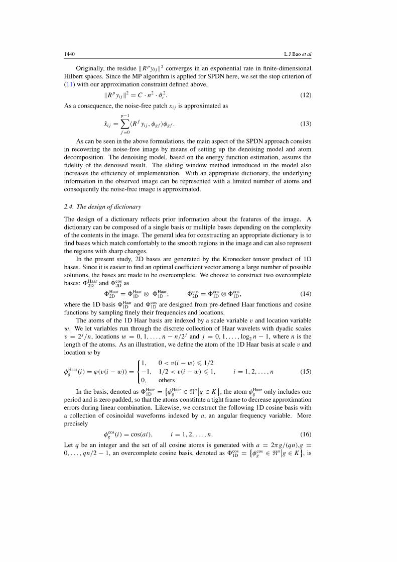
1440 L J Bao et al

Originally, the residue ‖Rpyij‖2 converges in an exponential rate in finite-dimensionalHilbert spaces. Since the MP algorithm is applied for SPDN here, we set the stop criterion of(11) with our approximation constraint defined above,

‖Rpyij‖2 = C · n2 · σ 2r . (12)

As a consequence, the noise-free patch xij is approximated as

xij =p−1∑f =0

〈Rf yij , φgf 〉φgf . (13)

As can be seen in the above formulations, the main aspect of the SPDN approach consistsin recovering the noise-free image by means of setting up the denoising model and atomdecomposition. The denoising model, based on the energy function estimation, assures thefidelity of the denoised result. The sliding window method introduced in the model alsoincreases the efficiency of implementation. With an appropriate dictionary, the underlyinginformation in the observed image can be represented with a limited number of atoms andconsequently the noise-free image is approximated.

2.4. The design of dictionary

The design of a dictionary reflects prior information about the features of the image. Adictionary can be composed of a single basis or multiple bases depending on the complexityof the contents in the image. The general idea for constructing an appropriate dictionary is tofind bases which match comfortably to the smooth regions in the image and can also representthe regions with sharp changes.

In the present study, 2D bases are generated by the Kronecker tensor product of 1Dbases. Since it is easier to find an optimal coefficient vector among a large number of possiblesolutions, the bases are made to be overcomplete. We choose to construct two overcompletebases: Haar

2D and cos2D as

Haar2D = Haar

1D ⊗ Haar1D ; cos

2D = cos1D ⊗ cos

1D , (14)

where the 1D basis Haar1D and cos

1D are designed from pre-defined Haar functions and cosinefunctions by sampling finely their frequencies and locations.

The atoms of the 1D Haar basis are indexed by a scale variable v and location variablew. We let variables run through the discrete collection of Haar wavelets with dyadic scalesv = 2j /n, locations w = 0, 1, . . . , n − n/2j and j = 0, 1, . . . , log2 n − 1, where n is thelength of the atoms. As an illustration, we define the atom of the 1D Haar basis at scale v andlocation w by

φHaarg (i) = ϕ(v(i − w)) =

⎧⎨⎩

1, 0 < v(i − w) � 1/2−1, 1/2 < v(i − w) � 1, i = 1, 2, . . . , n

0, others(15)

In the basis, denoted as Haar1D = {

φHaarg ∈ �n

∣∣g ∈ K}, the atom φHaar

g only includes oneperiod and is zero padded, so that the atoms constitute a tight frame to decrease approximationerrors during linear combination. Likewise, we construct the following 1D cosine basis witha collection of cosinoidal waveforms indexed by a, an angular frequency variable. Moreprecisely

φcosg (i) = cos(ai), i = 1, 2, . . . , n. (16)

Let q be an integer and the set of all cosine atoms is generated with a = 2πg/(qn),g =0, . . . , qn/2 − 1, an overcomplete cosine basis, denoted as cos

1D = {φcos

g ∈ �n∣∣g ∈ K

}, is

Denoising human cardiac diffusion tensor magnetic resonance images 1441

(a) (b)

Figure 2. Illustration of the generation of 2D bases. (a) 2D Haar basis constructed from 1D Haarbasis, (b) 2D cosine basis constructed from 1D cosine basis.

obtained. This is a q-fold overcomplete basis in which atoms are signals of consecutivecosinoidal waveforms.

Actually, the 2D bases are large arrays formed by taking all possible products between theelements of 1D bases. For instance, with the 1D basis Haar

1D of size n × √K , we can obtain

Haar2D of size n2 × K. Figure 2 depicts the generation of 2D bases. As shown in figure 2(a),

the atoms of Haar1D are of size n × 1 and they are a set of Haar waveforms with various scales

and locations. After implementing the Kronecker tensor product with other atoms, 2D atomsof size n × n are generated. For an image patch of size n × n, the 2D basis of size n2 × K isnecessary.

By comparing the Haar basis with the cosine basis in figure 2, it is observed that theintensity distributions of different atoms exhibit different geometrical structures. Atoms ofthe Haar basis are much sparser; as each atom has no more than three grey levels and itsenergy is just located in a local region of the atom. In contrast, the structure features ofcosine atoms are more complicated, as pixels in each atom include a wide range of grey levelschanging gradually in neighbourhood. Because of that, the Haar basis could perform wellin reconstructing images with piecewise constant contents or sharp changes while the cosinebasis has an advantage of representing images with piecewise smooth contents. The dictionaryconstructed in the present study consists of both 2D Haar basis and 2D cosine basis.

2.5. Segmentation as a prior

How to project an image on appropriate multiple-bases directly determines approximationaccuracy. One basis in the dictionary is generally efficient to represent one content whileineffective for representing the other contents. An image is usually composed of severalregions corresponding to different contents, so it is not useful to scan over the whole imagewith every basis in the dictionary. For that reason, we propose to use segmentation as aguide to locate the edges of regions with a given content and then choose appropriate basis toapproximate every contents. To segment an image, we use a detector based on the notion ofNSD (Liu et al 1995), which detects edges by measuring local NSDs.

As shown in figure 3, for an input signal S(i), a filter h1(i) operates on it, and then thevariation of the S(i) ∗ h1(i) is calculated:

δ2(i) = [S(i) ∗ h1(i)]2 ∗ h2(i) − [S(i) ∗ h1(i) ∗ h2(i)]

2, (17)

where h1(i) and h2(i) are linear normalized mean (i.e. rectangular) filters defined by

1442 L J Bao et al

2( )

2 ( )iδ2 ( )h i

2 ( )h i

2( )

( )iμ1( )h i

( )S i

Figure 3. Diagram of the nonstationary degree detector.

h1(i) = h2(i) = 1

Lrect

(i

L

), (18)

where L is the length of the filters.When the input signal is stationary at order 2, the output of such a detector is null.

Otherwise, the detector outputs higher values, indicating the presence of discontinuitiesbetween two stationary segments in the input signal.

For a 2D image, filters of size L × L are applied to calculate its NSD. Accordingly, theNSD of the input image is given by

δ2(i)[S(i) ∗ h1(i)]2 ∗ h2(i) − [S(i) ∗ h1(i) ∗ h2(i)]

2, (19)

where h1(i, j) and h2(i, j) are convolutions of two linear normalized mean filters

h(i, j) = h(i) ∗ h(j), with h(i) = 1

Lrect

(i

L

), h(j) = 1

Lrect

(j

L

). (20)

The output image δ2(i) gives prominence to the edges of the input image y, since the edgesbetween different regions represent nonstationary pixels. Therefore, it is easier to extract theedges of image y from image δ2(i) by the threshold method. For a volume data, to accountfor the spatial correlation in the neighbouring slices, the NSD detector can be extended to 3Dto achieve more efficient edge detection.

3. Materials and methods

3.1. Acquisition of human cardiac DT-MRI

The DT-MRI acquisitions on ex vivo human hearts were performed on the Hospital of Neuro-Cardiology of Lyon. We used a Siemens Avanto 1.5 T MR Scanner with a maximum gradientstrength of 40 mT m−1 and a slew rate of 200 T m−1 s−1. The sequence used is a DiffusionSpin Echo EPI, with a Stejskal-Tanner scheme and a b-value of 1000 s mm−2. Ten humanhearts were acquired including six healthy ones and four severely diseased ones (ischaemiccardiomyopathy). Each heart was located in a plastic container and fixed by hydrophilic gel tomaintain a diastolic shape. This setup has a low dielectric effect and also eliminates unwantedsusceptibility artefacts near the boundaries of the heart. In this paper, the LV (left ventricle)long axis, aligning with the axis of the magnet bore, is determined as the intersecting line ofthe two planes that divide the LV equally into four quadrants from base to apex. The shortaxis is defined perpendicular to the long axis.

We exercised DT-MRI acquisition protocols defined with different number of diffusiongradient directions ‘N’ and number of excitations ‘NEX’ as follows: (N, NEX) = (6, 1) and(30, 1). We used configurations of cuboctahedron and rhombicuboctahedron for the protocols

Denoising human cardiac diffusion tensor magnetic resonance images 1443

with 6 and 30 directions, respectively. Since DT-MRI acquisition for in vivo human heart isa great challenge because of cardiac and breathing motions, six gradient directions are moreappropriated in clinical application due to short acquisition time. However, high numbersof diffusion gradient directions are more immune to systematic artefacts and noise, withsignificantly increasing the precision of diffusion tensor and DAIs calculations and reducingrotational variance due to noise propagation (Landman et al 2007 Papadakis et al 2000).Jones (2004) demonstrated that at least 30 unique sampling orientations are required for arobust estimation of tensor orientation and MD. Therefore, we use ex vivo cardiac DT-MRIdata acquired with 6 diffusion directions and 30 diffusion directions to evaluate the proposedmethod.

The diffusion un-weighted image, a reference image, was acquired using the same DTIsequence with the diffusion gradient with b-value = 0 s mm−2. We perform the zonesegmentation of the heart with diffusion un-weighted images for their higher SNR and contrastcompared to DWIs. The other acquisition parameters were TE = 86 ms, TR = 8000 ms, slicethickness = 2 mm, slice spacing = 2 mm, slice duration = 130 ms, number of slices = 52.The volume data in each direction was arranged in a 128 × 128 × 52 array where spatialresolution of each voxel is 2 × 2 × 2 mm3.

3.2. Implementation of DT-MRI denoising

The acquired ex vivo human cardiac DT-MRI images mainly consist of two regions: thecardiac region of interest and the region outside the heart including black background andhydrophilic gel. The background corresponds to the air outside the organ and the variationrepresents noise. The intensity of the region with hydrophilic gel should be homogeneous in anoise-free image since the water molecules have the same diffusion character in such a region.Concerning the cardiac region, the information is more complex with anisotropic diffusion inmyocardium. Therefore, we choose to apply the Haar basis to the piecewise constant contentin the region outside the heart while using the cosine basis for the piecewise smooth contentin the heart region. We construct a dictionary composed of a Haar basis of size 64 × 196and a cosine basis of size 64 × 289. The images in each region, divided into overlappedpatches of size 8×8, are reconstructed after denoising using the denoising model presented insection 2.2.

Before that, the edges in the diffusion un-weighted image are detected by the NSDalgorithm. To take advantage of the spatial correlation in the neighbouring slices, two cubicfilters of size 3 × 3 × 3 are applied to the diffusion un-weighted image (figure 4(a)) and itstwo neighbouring slices. As described in section 2.5, the output of the first stage y ∗ h1 issimply the local mean value of the input image y while the output of the second stage δ2 is thevariance of this mean value. This method detects the edges in the diffusion un-weighted imageas shown in figure 4(b). Then, the edge between the two regions can be extracted by boundarytracking in MATLAB. Before that, we convert the image into a binary image based on a globalthreshold (14595 for figure 4(b)), estimated from the histogram of the image δ2(i, j) usingtwo-dimensional entropic thresholding (Abutaleb 1987). Thus, the obtained edge partitionsthe cardiac DWI into two regions: cardiac region of interest and the region outside the heart(figure 4(c)).

It is well known that the edge detection by thresholding is strongly affected by thecriterion for the selection of the threshold value. In the paper, we implement two-dimensionalentropic thresholding, which is based on the entropies of the grey level of the pixel and theaverage grey level of its neighbourhood. Since the NSD detector has enhanced the edges,the image δ2(i, j) presents high edge contrast. Therefore, it is feasible to detect the edge

1444 L J Bao et al

(a)

(b) (c)

Background

Gel

Myocardium

Ventricle cavity

Region 1

Region 2

Detected edge

Figure 4. Edge detection of cardiac DWI using the nonstationary degree detector. (a) The inputimage of the NSD: diffusion un-weighted image, (b) the output image of the NSD, (c) the DWI issegmented into two regions with the edge obtained from (b).

between the two regions using a global threshold. In experiments, two-dimensional entropicthresholding performs well on selecting a proper threshold and detects the edge without breaksor undesirable edge fragments. However, the double thresholding method, local thresholdingand also multi-stage thresholding may give more adaptive and robust results but they willincrease computation complexity and be more time consuming. Anyway, segmentation is anopen question and there are quite a number of segmentation methods. Among them, edgedetection by thresholding as we used is just a simple one and this is not our major topic.

It has been demonstrated that the noise in DWI presents a Rician distribution in whichrandom variable square is a non-central chi-square distribution. The means of two independentGaussian noises come from the real and imaginary channels of DT-MRI. Typical DWI containsa non-signal region in the background corresponding to the air outside the organ. In such aregion, it is assumed that x2 = 0 and the variances are all caused by noise. The Rician noiselevel σr used in (6) can be estimated by the square root of half expectation of the squared

intensity values in the non-signal regions of the corrupted image as σr =√

12E(y2) (Nowak

1999). For all the experiments in the cardiac DWIs, the same parameter setting has been usedfor factor C = 1.13, patch size 8 × 8 and filters size 3 × 3 × 3.

The effectiveness of the proposed method in denoising cardiac DT-MRI is compared withtwo conventional methods: PDE-based nonlinear diffusion denoising (Catte et al 1992) anda wavelet-based prior model from Pizurica et al (2003). The parameters of all the methods

Denoising human cardiac diffusion tensor magnetic resonance images 1445

have been experimentally optimized to produce the best denoising results with high SNRand contrast in profile. For PDE-based denoising, its parameters includes diffusion functiong(∇I ) = exp((‖∇I‖/k)−2), variance of Gaussian to convolve gradient and iteration number,while the parameters for the wavelet-based denoising are the threshold multiplication factorand window size (parameter definitions can be found in the above references).

3.3. Denoising performance evaluation

We generate a simulated heart-like-shaped image as shown in figure 5(a) to evaluate thebehaviour of the SPDN algorithm with the dictionary of multiple bases and the NSD detector.The simulated heart-like-shaped image presents two structures: the central part of the imageexhibits a heart shape akin to left and right ventricles while the rest of the image representsthe gel and air regions in cardiac DWI. The intensity of the left ventricular region is made tochange gradually from inside to outside to simulate the diffusion difference of the fibresfrom the endocardium to the epicardium. We corrupt the simulated image with Riciannoise of different levels σr ∈ {5, 10, 15, 20, 25, 30} with respect that the intensity of thenoise-free image ranges from 0 to 221. As the noise-free image is known in advance fora simulated image, the SNR is defined as (Pizurica et al 2003, Awate and Whitaker 2007)10 · log10(Var(x)/Var(x−x)), where Var(·) denotes the variance of the intensities of the image,x the noise-free image and x either the noisy image y or the denoised image x as defined insection 2.2.

To assess the performance of the proposed denoising method on cardiac DWIs, the SNRcalculated on DWIs is the most intuitive measurement. Since we do not know the ground truthof cardiac DWIs, the SNRs of the cardiac DWIs are computed over two regions of interest(ROI). The conventional MR image SNR criterion is SNR = 10 · log10

(x2

mean

/σ 2

r

)(Nowak

1999), where xmean designates the mean of the intensity in the ROI of the myocardium, andσr denotes the standard deviation of the noise calculated from the air region in the image. Inaddition, we also propose to apply another definition SNR 2 = 10 · log10

(σ 2

M

/σ 2

G

)in order

to account for the very granular aspect of our DWIs and blurring effects in different regionseventually produced by denoising algorithms. In this definition, we measure a signal varianceto noise variance ratio, where σ 2

M denotes the variance of the signal in the ROI of myocardiumand σ 2

G denotes the variance of the noise in the ROI of the gel region. Because the intensity ofthe gel region in DWI is homogeneous in principle as discussed in section 3.2, this leads us tocalculate the noise from the intensity variance of the gel in this definition.

To further get insights into the denoising performance of the proposed method, a set ofslices are selected around the equatorial slice of each heart to measure the DT-MRI indicesbefore and after denoising. In the paper, the FA map, MD map, directionality map andfibre architecture are employed to qualitatively illustrate the different performance of the threedenoising methods. Furthermore, we apply the quantitative statistics on the negative eigenvaluecount, mean and variance (Var) of FA, MD, CI and fibre length to give a comprehensiveanalysis. These maps and their corresponding statistical analyses are implemented withsoftware Bioimagesuite (Papademetris et al http://www.bioimagesuite.org).

In the presence of noise and artefacts, the tensors at some voxels may yield negativeeigenvalues that are not physically possible and we should exclude these voxels from thediffusion maps and statistics. Denoising allows decreasing the number of voxels with negativeeigenvalues. FA and MD are two parameters derived from the non-negative eigenvalues ofdiffusion tensors, which describe the anisotropy and the diffusivity of diffusion, respectively.FA measures the variability of water mobility in different directions and is defined asFA ={ 3[(λ1−λ)2+(λ2−λ)2+(λ3−λ)2]

2(λ21+λ2

2+λ23)

}1/2, where λ is quantified as the mean of the three eigenvalues

1446 L J Bao et al

(a) (b)

(c) (d) (e)

20 40 60 80 100 1200

50

100

150

200

250

noise free

SPDN

PDE-based

wavelet-based

(f)

Figure 5. Denoising results on the simulated image with the Rician noise level σr = 20.(a) Noise-free image. (b) Noisy image, SNR = 13.8 dB. Images denoised using (c) SPDN,SNR = 17.9 dB, (d) PDE-based nonlinear diffusion denoising, SNR = 17.7 dB and (e) wavelet-based denoising, SNR = 16.7 dB. The line profiles corresponding to images (a) and (c)–(e) areshown in (f). Pixels around the arrow heads in images (d) and (e) exhibit obvious fine structurelosses and artefacts, and pixels in the circles in (f) are differences to be noted in denoising results.

of the diffusion tensor λ1, λ2, λ3. It ranges from 0 for isotropic diffusion to 1 for completelyanisotropic diffusion. MD, denoted as λ, indicates the mean diffusivity of water molecules,which reflects the redistribution of intracellular and extracellular space volumes.

Directionality map, CI and fibre reconstruction all reflect the orientation distribution ofdiffusion tensors defined by the principal eigenvectors. Directionality map, also called thecolour tensor, represents the principal eigenvector by means of a colour representation: the x

Denoising human cardiac diffusion tensor magnetic resonance images 1447

5 10 15 20 25 3010

15

20

25

30

Noise standard deviation

SN

R(d

B)

noisy image

SPDN denoised

PDE denoised

wavelet denoised

Figure 6. Comparison of denoising results obtained with the three methods in terms of SNR inthe case of the simulated image with different noise levels σr ranging from 5 to 30.

(left–right) component as red, the y (anterior–posterior) component as green and the z (apex–base) component as blue, and the brightness is modulated by FA in the paper. CI estimatesthe orientation coherence of fibres and is defined as the mean dot product CI = 1

26

∑ij v · vij

of the eigenvectors v and its 26 neighbouring voxels vij . A high CI value reflects directionalcoherence of fibres in neighbouring voxels. It is well known that the heart fibre represents ahelix structure with the transmural gradient of fibre inclination angles. Fibre regularity, fibrecount and also fibre lengths and angles are important information in DT-MRI applications.

4. Results

4.1. Application to simulated images

Figures 5(a) and (b) show the simulated noise-free and noisy (σr = 20) images. Infigure 5(a), the contour in green represents the edge obtained with the NSD detector. Theresults of denoising using the different methods are illustrated in figures 5(c)–(e) and theirprofiles’ comparison are shown in figure 5(f). The SNR of the denoised image in figure 5(c) isimproved by 4.1 dB compared to the corrupted image, while the PDE-based denoising increasesthe SNR by 3.9 dB and the wavelet-based filter increases the SNR by 2.9 dB as represented infigures 5(d) and (e).

The proposed SPDN method (figure 5(c)) almost suppresses the noise while keeping avery good spatial resolution (sharper edges are preserved) and high contrast (the denoisedimage almost has the same dynamic range as the original image). In contrast, PDE-baseddenoising leads to more fine structure losses (see the region indicated by the arrow infigure 5(d)) and its contrast preservation is also worse than SPDN as can be observed inthe peaks and valleys of the profile shown in figure 5(f). On the other hand, wavelet-baseddenoising introduces obvious artefacts, especially in the high intensity region as indicated bythe two arrows in figure 5(e). SPDN leads to less contrast loss and fewer artefacts than theother two methods. This is particularly clear when comparing their profiles in figure 5(f).More quantitatively, figure 6 gives the comparison between the three methods in terms of SNRfor different noise levels. It is seen that the proposed method and PDE-based method alwaysyield better results than the wavelet-based method except for the noise level σr = 30, to whichthe obtained SNRs are close.

1448 L J Bao et al

(a) (b)

(c) (d)

ROI

Figure 7. Denoising results on a DWI of ex vivo human cardiac DT-MRI datasets with (N, NEX) =(6, 1) (a) Noisy DWI with SNR = 18.2 dB, SNR 2 = 4.5 dB. Image denoised using (b) SPDN,SNR = 25.4 dB, SNR 2 = 10.4 dB; (c) PDE-based smoothing, SNR = 24.3 dB, SNR 2 =8.2 dB; and (d) wavelet-based filter, SNR = 23.2 dB, SNR 2 = 6.6 dB. The line profiles in (e)–(h)correspond to the images in (a)–(d).

4.2. Application to human cardiac DT-MRI

The results of denoising the real DWIs using the proposed method and PDE- and wavelet-based denoising techniques are demonstrated in figure 7. Figure 7(a) represents a DWI ofex vivo diseased human cardiac DT-MRI data with (N, NEX) = (6, 1). The proposedmethod (figure 7(b)) produces the best performance with the highest SNRs (SNR = 25.4 dB,SNR 2 = 10.4 dB) as the ROI marked in figure 7(a). This ROI corresponds to the myocardialregion of the left ventricle. In contrast, the PDE-based method presents some ‘washing effect’by drastically modifying the grey level aspect of the original image and details and its SNRsof the result are SNR = 24.3 dB, SNR 2 = 8.2 dB. Concerning the wavelet-based method,it gives results visually similar to those of the proposed method, but with smaller SNRs(SNR = 23.2 dB, SNR 2 = 6.6 dB). The performance difference between the three methodscan be further assessed with the profiles in figures 7(e)–(h). Using a PC with Intel Pentium

Denoising human cardiac diffusion tensor magnetic resonance images 1449

20 40 60 80 100 1200

50

100

150

200

250

20 40 60 80 100 1200

50

100

150

200

250

(e) (f)

20 40 60 80 100 1200

50

100

150

200

250

20 40 60 80 100 1200

50

100

150

200

250

(g) (h)

Figure 7. (Continued.)

Dual E2140 1.60 GHz, 2.00 GB memory, windows XP platform, it takes about 4 min and 20 sfor denoising a 3D DT-MRI dataset of size 128 × 128 × 52 using the proposed method.

Figures 8 and 9 show the FA maps, MD maps and directionality maps of a slice of theheart in figure 7 with (N, NEX) = (6, 1) and (30, 1), respectively, calculated before andafter denoising with the three methods. Their quantitative analyses are given in table 1. Infigure 8(a), the FA map before denoising exhibits noticeable noise-induced granular aspectsand even black stains because of negative eigenvalue, which are also present in the MDmaps (figure 8(b)) and directionality maps (figure 8(c)). With PDE-based and wavelet-baseddenoising, many graininess artefacts remain with high FA and the negative eigenvalues arealmost not removed. In contrast, SPDN removes most of the negative eigenvalues and artefactsin the maps. The directionality maps indicate that the principle eigenvectors are more regularlyoriented as the colour of neighbouring voxels changes gradually with less discontinuity afterdenoising the DWIs using the proposed method. Note that the maps with (N, NEX) = (30, 1)exhibit the same problems, but that granular aspects and negative eigenvalues are less severethan in the maps derived from (6, 1), as can be observed in figure 9. It is found that SPDNdenoising yields the visually best maps than the other two methods, by removing more negativeeigenvalues and regularizing the direction distribution of diffusion tensors.

The above visual analyses are confirmed by the quantitative results in table 1. We observethat denoising decreases the number of negative eigenvalues (the number of voxels withpositive eigenvalue is denoted by ‘Available voxels’ in the tables) and the FA mean and its

1450 L J Bao et al

(a)

(b)

x (red)

y (green)

z (blue)

(c)

Figure 8. DT-MRI index maps of a diseased heart of scheme (6, 1). (a) FA maps, (b) MD(10−3 mm2 s−1) maps and (c) directionality maps. From left to right, the maps correspond to noisyDT-MRI, and denoised DT-MRIs obtained with SPDN, PDE-based and wavelet-based denoising,respectively.

variance while increasing the CI mean. Moreover, the indices of scheme (6, 1) after denoisingapproximate to the values of (30, 1). For instance, after denoising the data of scheme (6, 1)with SPDN, its FA mean decreases from 0.443 to 0.350, compared with the value of 0.429and 0.414 for the other methods, 0.350 being the closest to the FA mean (0.300) of (30, 1).Generally, among the three methods, the SPDN produces the most significant improvementson indices: −21% for FA mean, −3% for MD mean and 52% for CI mean for data of scheme(6, 1). The denoising effect on the data of scheme (30, 1) are −13% for FA mean, −1% forMD mean and 28% for CI mean. Meanwhile, the decrease of MD is tiny compared with theother indices.

Denoising human cardiac diffusion tensor magnetic resonance images 1451

(a)

(b)

x (red)

y (green)

z (blue)

(c)

Figure 9. DT-MRI index maps of the same diseased heart in figure 8, but of scheme (30, 1).(a) FA maps, (b) MD (10−3 mm2 s−1) maps and (c) directionality maps. From left to right, themaps correspond to noisy DT-MRI, and denoised DT-MRIs obtained with SPDN, PDE-based andwavelet-based denoising, respectively.

Figure 10 renders the fibres (in directionality colour map) of the heart with ten slicesaround the slice in figure 7. Table 2 gives the indices of the fibres. The following thresholdsare used in fibre tracking: FA 0.05 (this FA threshold was chosen empirically in order to trackmore fibres), minimum fibre length 5 mm and maximum fibre angle 60◦. We observe thatwithout denoising, the tracked fibres are in disorder and intermittent, while after denoising,fibre tracking can smoothly construct the curvature of the trajectories, especially for thedata of scheme (6, 1) in figure 10(a). Compared with original 2851 fibres before denoising(figure 10(a) left), a number of 3123 fibres are tracked from cardiac DT-MRI denoised with

1452 L J Bao et al

(a)

(b)

x (red)

y (green)

z (blue)

Figure 10. Myocardium fibre tracking before and after denoising the heart shown in figures 8and 9, with (a) the DT-MRI of scheme (6, 1) and (b) of scheme (30, 1). Left column: with noisyDT-MRIs. Right column: with DT-MRIs denoised using SPDN.

SPDN (figure 10(a) right) and the mean of fibre length increases from 6.6 mm to 7.6 mm.The fibres also run more regularly with the mean of fibre angle decreased from 16.2◦ to 12.2◦

and are more consistent with fibre organization reconstructed from the data of scheme (30, 1)(figure 10(b)). As for DT-MRI data of scheme (30, 1), denoising with the proposed methodmakes the fibre architecture more delicate and precise, providing more structure details withmore tracked fibres as listed in table 2.

Finally, denoising results on the other nine hearts of scheme (30, 1) (three slices of eachheart) with the proposed method are reported in table 3. The results are consistent with thosein table 1: the decrease of FA mean and MD mean range from −3% to −21% and 0 to −4%while the increase of CI mean ranges from 5 to 39%. It is interesting to note that, in table 3,the MD means of the diseased heart are higher than the normal hearts.

Denoising human cardiac diffusion tensor magnetic resonance images 1453

Table 1. Comparison of the denoising methods in terms of available voxels, fractional anisotropy,mean diffusivity and fibre coherent index, for the images shown in figures 8 and 9.

FA MD (10−3 mm2 s−1) CIVoxels Available

Samples in mask voxels Mean Var Mean Var Mean Var

(6, 1) Noisy 668 613 0.443 0.027 0.983 0.094 0.653 0.091SPDN 656 0.350 0.023 0.957 0.092 0.992 0.123PDE-based 621 0.429 0.027 0.976 0.097 0.701 0.097Wavelet-based 656 0.414 0.026 0.974 0.082 0.743 0.106

(30, 1) Noisy 677 670 0.300 0.021 0.827 0.089 0.938 0.129SPDN 674 0.261 0.018 0.818 0.090 1.198 0.118PDE-based 670 0.292 0.020 0.826 0.090 0.944 0.133Wavelet-based 670 0.283 0.020 0.826 0.089 1.003 0.131

Table 2. Quantitative analysis of the fibre architectures shown in figure 10. For each scheme, thefirst line corresponds to the DT-MRI data before denoising and the second line to the data afterdenoising using SPDN.

FA MD (10−3 mm2 s−1) Fibre length (mm) Fibre angle (◦)Fibre Volume

Samples count (mm3) Mean Var Mean Var Mean Var Mean Var

(6, 1) 2851 8551 0.360 0.010 0.769 0.028 6.615 30.734 16.210 16.4213123 8987 0.296 0.009 0.750 0.026 7.593 31.222 12.262 16.171

(30, 1) 3069 8885 0.271 0.008 0.635 0.024 6.236 22.305 10.416 16.6853155 8956 0.245 0.007 0.627 0.024 6.202 19.875 8.170 13.755

5. Discussion and conclusion

As observed in the preceding section, after denoising the DT-MRI, the FA mean and its variancedecrease and the CI mean increases obviously. It also alters fibre tracking by increasing thenumber of tracked fibres and fibre lengths. These are in agreement with the observationsreported in previous studies (Basser and Pajevic 2000, Koay et al 2007) that the presenceof noise induce negative eigenvalues, positive error in FA, disorder of the eigenvectors andtracked fibres. These errors in DT-MRI indices are all because of the bias in the principaleigenvalues and principal eigenvectors calculated from the noisy DT-MRI.

However, as two diffusion indices are computed from eigenvalues, it is observed that MDmeans vary a little before and after denoising while FA means change a lot. This is due to thedefinition of the two indices. So FA is intrinsically more susceptible to noise contaminationthan MD, as reflected by its larger bias and error variance for the same SNR levels (Basserand Pierpaoli 1998). We can also find that the denoising effects on the indices of scheme(6, 1) are more obvious than those of (30, 1) and denoising makes the indices of scheme (6, 1)approximate to those of (30, 1). This is because a high number of diffusion gradient directionsand longer acquisition time are more immune to systematic artefacts and noise. Therefore,DT-MRI indices generated from data of scheme (30, 1) provide references for evaluating thedenoising performance on data of scheme (6, 1).

As indicated in table 3, the MD means for a diseased heart are higher than the normalhearts. This finding is consistent with the findings of the DT-MRI study of Wu and Tseng(2006). They report that FA will decrease if the organization of tissue structure is destroyed and

1454 L J Bao et al

Table 3. Results of denoising using SPDN on the other nine hearts of scheme (30, 1). For eachheart, the first line corresponds to the DT-MRI data before denoising and the second line to thedata after denoising using SPDN.

MD (10−3

FA mm2 s−1) CIVoxel Available

Heart in mask voxel Mean Var Mean Var Mean Var

Normal 1 3057 2923 0.326 0.024 0.654 0.113 1.000 0.1013057 0.303 0.025 0.624 0.118 1.195 0.115

Normal 2 2375 2314 0.338 0.023 0.633 0.174 0.951 0.1472344 0.293 0.019 0.624 0.172 1.233 0.141

Normal 3 2373 2370 0.223 0.008 0.596 0.041 1.123 0.1462372 0.216 0.007 0.598 0.040 1.173 0.146

Normal 4 2827 2820 0.302 0.013 0.587 0.089 0.823 0.2112826 0.252 0.007 0.578 0.085 1.141 0.316

Normal 5 2056 2039 0.270 0.015 0.699 0.058 1.010 0.1262046 0.244 0.012 0.696 0.055 1.197 0.125

Normal 6 3086 3059 0.253 0.017 0.800 0.118 0.831 0.1593075 0.209 0.013 0.789 0.118 1.137 0.202

Diseased 1 2683 2668 0.312 0.018 0.836 0.073 0.987 0.1232679 0.259 0.016 0.832 0.067 1.118 0.124

Diseased 2 2666 2659 0.270 0.012 0.760 0.038 1.097 0.1112664 0.213 0.008 0.770 0.037 1.418 0.068

Diseased 3 2059 2002 0.303 0.022 0.821 0.090 0.919 0.1092020 0.263 0.018 0.811 0.091 1.148 0.106

MD is significantly increased in the infarct (ischaemia) zone in the human heart. Endocardialarea is most susceptible to ischaemia. Therefore, positive angles had the most severe loss inthe infarct zone. Since the exact ischaemia zones are unknown for us now, more researchesare necessary for demonstrating that.

We compare the proposed method with two common filters for denoising DT-MRI.According to the results, our proposed method consistently outperforms the PDE- and wavelet-based filters in both qualitative and quantitative analyses. The method we have proposedfor denoising human cardiac DT-MRI is based on combining sparse representation with asegmentation scheme using the NSD detector. The sparse representation exploits the uniqueproperty of atom decomposition to reconstruct the underlying noise-free image. The use ofthe NSD detector allows the different contents of the image to be segmented, which makesthe generation of the dictionary more adaptive and also improves the denoising result. Theobtained results show that the proposed method effectively reduces the noise in human cardiacDT-MRI while preserving image details and contrast and improving the calculation accuracyof diffusion tensors as well as the principal eigenvector field of the heart. That would allow amore precise and robust fibre tracking of the myocardium. In the future work, the proposeddenoising method can be further optimized by designing more specific dictionaries with respectto the particular features of human cardiac DWIs, or by extending the SPDN method to 3Ddata.

In the proposed denoising method, there are three adjustable parameters: factor C in (8),patch size and filter window size L. The parameter C influences the denoising results, butrather slightly. C should be greater than 1. However, when C is too great, over-filtering canoccur. In practice, the values of C between 1.05 and 1.15 yield similar denoising results,as the SNR difference between the denoised results obtained with C = 1.15 and 1.05 is less

Denoising human cardiac diffusion tensor magnetic resonance images 1455

than 0.05 dB for the simulated images while the differences of SNR and SNR 2 are less than0.3 dB and 0.2 dB separately for real cardiac images. In our experiments, setting C = 1.13achieves the near optimal results for real cardiac images with a tradeoff between SNR andSNR 2. Concerning the patch size, it is, in the field of image processing, well known thatspatial correlation in an image does not exceed 16 × 16. Therefore, one often simply choosesa patch size among 8 × 8, 16 × 16 and 32 × 32. In our present study, 8 × 8 is a good choice interms of denoising effects (SNR and contrast in profile) and computation time (a larger patchsize will be more time-consuming with rather close results). As for the filter window size L,it is generally chosen as 3, 5 or 7 according to the image in question. Here we use filters ofsize 3 × 3 × 3 for cardiac DT-MRI and 3 × 3 for a simulated image since they produced thebest edge enhancement for the images studied.

The objective of the proposed segmentation is to obtain the myocardium region. Theproposed segmentation process is based on using the notion of NSD, which is particularlypowerful for detecting the presence of discontinuities between two regions in the inputimage. For the ex vivo cardiac DT-MRI data investigated in the present study, the proposedsegmentation always works well on the diffusion un-weighted image. In principle, it couldstill work in case greater contrast variations are present throughout the image. This aspectshould be further investigated for in vivo human cardiac DT-MRI. However, no matter forin vivo and ex vivo cardiac image, it is better to apply segmentation as a guide to the choice ofthe basis when denoising cardiac DT-MRI using the SPDN method. It also supplies an ideafor using SPDN to general image processing.

Acknowledgments

This work is supported by the National Natural Science Foundation of China (60777004)and International S&T Cooperation Project of China (2007DFB30320). The authors thankStanislas Rapacchi for his help in acquiring the data, and many other researchers in CREATIS-LRMN for their helpful discussions and comments in this investigation.

References

Abutaleb A S 1987 Automatic thresholding of gray-level pictures using two dimensional entropy Comput. Vis. Graph.Image Process. 47 22–32

Aharon M, Elad M and Bruckstein A 2006 K-SVD: an algorithm for designing overcomplete dictionaries for sparserepresentation IEEE Trans. Signal Process. 54 4311–22

Alexander M E, Baumgartner1 R, Summers A R, Windischberger C, Klarhoefer M, Moser E and Somorjai R L2000 A wavelet-based method for improving signal-to-noise ratio and contrast in MR images Magn. Reson.Imaging 18 169–80

Arsigny V, Fillard P, Pennec X and Ayache N 2006 Log-Euclidean metrics for fast and simple calculus on diffusiontensors Magn. Reson. Med. 56 411–21

Awate S P and Whitaker R T 2007 Feature-preserving MRI denoising: a nonparametric empirical Bayes approachIEEE Trans. Med. Imaging 26 1242–55

Basser P J, Mattiello J and LeBihan D 1994 MR diffusion tensor spectroscopy and imaging Biophys. J. 66 259–67Basser P J and Pajevic S 2000 Statistical artifacts in diffusion tensor MRI (DTMRI) caused by background noise

Magn. Reson. Med. 44 41–50Basser P J and Pierpaoli C 1998 A simplified method to measure the diffusion tensor from seven MR images Magn.

Reson. Med. 39 928–34Basu S, Fletcher T and Whitaker R 2006 Rician noise removal in diffusion tensor MRI MICCAI LNCS 4190 117–25Catte F, Lions P L, Morel J M and Coll T 1992 Image selective smoothing and edge detection by nonlinear diffusion

SIAM J. Numer. Anal. 29 182–93Chen B and Edward W 2005 Noise removal in magnetic resonance diffusion tensor imaging Magn. Reson. Med.

54 393–407

1456 L J Bao et al

Chen S S, Donoho D L and Saunders M A 1998 Atomic decomposition by basis pursuit SIAM J Sci. Comput. 20 33–61Elad M and Aharon M 2006 Denoising via sparse and redundant representations over learned dictionaries IEEE Trans.

Image Process. 15 3736–45Galban C J, Maderwald S, Uffmann K and Ladd M E 2005 A diffusion tensor imaging analysis of gender differences

in water diffusivity within human skeletal muscle NMR Biomed. 18 489–98Gerig G and Kubler O 1992 Nonlinear anisotropic filtering MRI data IEEE Trans. Med. Imaging 11 221–33Gilboa G, Sochen N and Zeevi Y Y 2004 Image enhancement and denoising by complex diffusion processes IEEE

Trans. Pattern Anal. Mach. Intell. 26 1020–36Gorodnitsky I F and Rao B D 1997 Sparse signal reconstruction from limited data using FOCUSS: a re-weighted

minimum norm algorithm IEEE Trans. Signal Process. 45 600–16Granai L and Vandergheynst P 2004 Sparse decomposition over multi-component redundant dictionaries IEEE Proc

of Multimedia Signal Processing, Workshop on MMSPGudbjartsson H and Patz S 1995 The Rician distribution of noisy MRI data Magn. Reson. Med. 34 910–4Guleryuz O G 2005a Nonlinear approximation based image recovery using adaptive sparse reconstructions and

iterated denoising: part I. Theory IEEE Trans. Image Process. 15 539–53Guleryuz O G 2005b Nonlinear approximation based image recovery using adaptive sparse reconstructions and

iterated denoising: part II. Adaptive algorithms IEEE Trans. Image Process. 15 554–71Hamarneh G and Hradsky J 2007 Bilateral filtering of diffusion tensor magnetic resonance images IEEE Trans. Image

Process. 16 2463–75Jones D K 2004 The effect of gradient sampling schemes on measures derived from diffusion tensor MRI: a Monte

Carlo study Magn. Reson. Med. 51 807–15Koay C G, Chang L C, Pierpaoli C and Basser J P 2007 Error propagation framework for diffusion tensor imaging

via diffusion tensor representations IEEE Trans. Med. Imaging 26 1017–34Landman B A, Farrell J D, Jones C K, Smith S A, Prince J L and Moria S 2007 Effects of diffusion weighting

schemes on the reproducibility of DTI-derived fractional anisotropy, mean diffusivity, and principal eigenvectormeasurements at 1.5 T NeuroImage 36 1123–38

Liu W Y, Magnin I E and Gimenez G 1995 Un nouvel operateur pour la detection de rupture dans des signaux bruitesTrait. Signal 12 226–36

Macovski A 1996 Noise in MRI Magn. Reson. Med. 36 494–7Mallat S and Zhang Z 1993 Matching pursuits with time-frequency dictionaries IEEE Trans. Signal Process.

41 3397–415Nowak R D 1999 Wavelet based Rician noise removal for magnetic resonance imaging IEEE Trans. Image

Process. 8 1408–19Papadakis N G, Murrills C D, Hall L D, Huang C L and Carpenter T A 2000 Minimal gradient encoding for robust

estimation of diffusion anisotropy Magn. Reson. Imaging 18 671–9Papademetris X, Jackowski M, Rajeevan N, Constable R T and Staib L H BioImage Suite: an integrated medical

image analysis suite Section of Bioimaging Sciences, Department of Diagnostic Radiology, Yale School ofMedicine http://www.bioimagesuite.org

Perona P and Malik J 1990 Scale-space and edge-detection IEEE Trans. Pattern. Anal. Mach. Intell. 12 629–39Pham T V and Smeulders A W M 2006 Sparse representation for coarse and fine object recognition IEEE Trans.

Pattern. Anal. Mach. Intell. 28 555–67Pizurica A, Philips W, Lemahieu I and Acheroy M 2003 A versatile wavelet domain noise filtration technique for

medical imaging IEEE Trans. Med. Imaging 22 323–31Schwartz E D, Duda J, Shumsky J S, Cooper E T and Gee J 2005 Spinal cord diffusion tensor imaging and fiber

tracking can identify white matter tract disruption and glial scar orientation following lateral funiculotomyJ. Neurotrauma 22 1388–98

Scollan D F and Holmes A 2000 Reconstruction of cardiac centricular geometry and fiber orientation using magneticresonance imaging Ann. Biomed. Eng. 28 934–44

Starck J L, Elad M and Donoho D L 2005 Image decomposition via the combination of sparse representations and avariational approach IEEE Trans. Image Process. 14 1570–82

Wirestam R and Bibic A 2006 A denoising of complex MRI data by wavelet-domain filtering: application tohigh-B-value diffusion-weighted imaging Magn. Reson. Med. 56 1114–20

Wu M T and Tseng W Y 2006 Diffusion tensor magnetic resonance imaging mapping the fibre architecture remodellingin human myocardium after infarction Circulation 114 1036–45