CHEM 2070 Structure And Spectroscopy

Summer 2005

Michael K. Denk

NMR Spectroscopy

NMR Spectroscopy Nuclear Magnetic Resonance (NMR), first discovered in 1945, has evolved into one of

the premier techniques for molecular identification. NMR has become a crucial tool for

chemical research, biochemistry, pharmaceutical chemistry, polymer science, petroleum research, agricultural chemistry and medicine

NMR Spectrometers

NMR spectrometers combine three building blocks

• A strong magnetic field • A radio frequency generator • A radio frequency detector

NMR spectrometers are commerically available (0.1 - 10 Mega $ ) from:

• Varian Inc. • Bruker • JEOL (Japan Electron Optics Laboratory Inc.)

Modern NMR spectrometers rely on three revolutionary developments:

• Pulse NMR • Fourier Transform data acquisition • 2D NMR techniques

The investigation of living tissue (uncluding humans) requires special spectrometers, the technique is called

• Magnetic Resonance Imaging (MRI)

NMR Spectroscopy on the WWW

NMR Spectroscopy is now used in so many disciplines that the true breadth of the method cannot be covered in a introductory lecture. The hyperlinks below lead to important NMR centers and should give you a first impression of NMR and its many applications.

Infromation about our own NMR center:

NMR Center University of Guelph

Other hyperlinks:

An Introduction to Magnetic Resonance (Word.doc, Uni-Duisburg) NMR Center Heidelberg (Germany) Bruker WWW Server | Bruker ftp server | Frequently Asked Questions Protein NMR Structures (Oxford) Slovenian NMR Center NMR Information Server Univ. of Florida. NMR Center Madison (Wisconsin, USA) | NMR Pulse sequences | Meetings of Interest to the NMR Community BioMagResBank Database for Protein, Peptide, and Nucleic Acid Structural Data Derived by NMR Spectroscopy NMR Spectroscopy. Principles and Application(ICSTM Chemistry Department, UK) NMR Center University of Florida NMR Manuals for Bruker Instruments (Uni-Duisburg)

Documents on NMR Theory (Uni-Duisburg) (MS-Winword files)

Electron Spin: Theory Goudsmit and Uhlenbeck postulated (1925), that the of splitting of certain spectral lines in an external magnetic field is due to an "electron spin" (which causes a constant magnetic moment of the electron).

The assumption of an electron spin can readily explain the observed fine structure if one assumes that the spin s (+1/2 or -1/2) combines with the orbital momentum m to give a total momentum j .

j = m + s

It is this total momentum that must now change by ±1 to absorb the photon's spin, in other words we have a refined selection rule:

j = ±1

The electron spin is not delivered by the Schrödinger equation but follows from a more refined version that was developed by Paul Dirac and that includes relativity.

Paul Dirac 1902-1984

Nobel Prize 1933 (Physics)

Electron Spin: Experiment

The first experimental evidence for the existence of an electron spin came from the Stern-Gerlach experiment which involved the the deflection of a beam of silver atoms in an inhomogeneous magnetic field.

Silver atoms possess the valence shell of 4d10 5s1. The ten d electrons are all paired, but the spin of the 5s electron is not. If silver atoms are shot at a target, they produce a single broad spot. However, in the presence of an external inhomogeneous magnetic field, two spots are observed (O. Stern, Z. Phys. 1921, 7, 249; O. Stern, W. Gerlach, Ann. Phys. 1924, 74, 63).

Otto Stern 1888 - 1969

Nobel Prize 1943 (Physics)

Nuclear Spin: Postulate

Nuclear Magnetic resonance has the distinction to be the brainchild of no less than five Nobel prize winners.

Wolfgang Pauli postulated the existence of a nuclear spin [1] to explain the so called hyperfine structure of atomic spectra even before he "invented" electron spin (the 4th quantum number).

"Following Bohr's invitation, I went to Copenhagen in the autumn of 1922, where I made a serious effort to explain the so-called « anomalous Zeeman effect », as the spectroscopists called a type of splitting of the spectral lines in a magnetic field which is different from the normal triplet...

...The gap was filled by Uhlenbeck and Goudsmit's idea of electron spin, which made it possible to understand the anomalous Zeeman effect simply by assuming that the spin quantum number of one electron is equal to 1/2 and that the quotient of the magnetic moment to the mechanical angular moment has for the spin a value twice as large as for the ordinary orbit of the electron. Since that time, the exclusion principle has been closely connected with the idea of spin...

...In 1925, the same year in which I published my paper on the exclusion principle, De Broglie formulated his idea of matter waves and Heisenberg the new matrix-mechanics, after which in the next year Schrödinger's wave mechanics quickly followed. It is at present unnecessary to stress the importance and the fundamental character of these discoveries, all the more as these physicists have themselves explained, here in Stockholm, the meaning of their leading ideas

W. Pauli, Nobel Lecture, December 13, 1946

1. W. Pauli, Naturwissenschaften, 1924, 12, 741.

Nuclear Spin: First Experiments

The existence of a nuclear spin was confirmed experimentally by Rabi in 1939.

The Rabi experiment showed that a beam of hydrogen molecules passing through a magnetic field absorbs radio frequency of a discrete wavelength.

The experiment is very similar to the Stern-Gerlach experiment but uses the absorption of radio waves to demonstrate the formation of a 2-level system.The experiment is thus not only proof for the existence of a nuclear spin but was also the first magnetic resonance experiment. Rabi received the Nobel Prize in Physics, 1944 "for his resonance method for recording the magnetic properties of atomic nuclei" (Original papers by Rabi et al.: 1 | 2| 3)

Other Nobelprize winners associated with NMR:

Wolfgang Pauli 1900 - 1958

Nobel Prize 1945 (Physics)

Isidor Isaac Rabi 1898 - 1988

Nobel Prize 1944 (Physics)

Felix Bloch 1905 - 1983

Nobel Prize 1955 (Physics)

Edward Purcell 1912 - 1997

Nobel Prize 1955 (Physics)

Richard Ernst 1933-

Nobel Prize 1991 (Chemistry)

John B. Fenn

1917-

Nobel Prize 2002

(Chemistry)

Koichi Tanaka

1959-

Nobel Prize 2002

(Chemistry)

Kurt Wüthrich

1938-

Nobel Prize 2002

(Chemistry)

NMR - The First Experiments

The first NMR experiment on condensed matter was carried out by Felix Bloch (Zürich & Stanford) and Edward Purcell (Harvard) who were jointly awarded the 1952 Nobel Prize in Physics for their discovery.

1. F. Bloch, W. Hansen, M. E. Packard, Phys. Rev. 1946, 69, 127. 2. E. M. Purcell, H. C. Torrey, R. V. Pound, Phys. Rev. 1946, 69, 37.

The interest of chemists in NMR was limited until it was observed (1949-1950) that the chemical environment leads to a specific shift in the resonance frequency ("chemical shift")

1. W. D. Knight, Phys. Rev. 1949, 76, 1259. 2. W. G. Proctor, F. C. Yu, The Dependence of a Nuclear Magnetic Resonance Frequency

upon Chemical Compound Phys. Rev. 1950, 77, 717. 3. W. C. Dickinson, "Dependence of the F19 Nuclear Resonance Position on Chemical

Compound" Phys. Rev. 1950, 77, 736-737. 4. G. Lindström, Phys. Rev. 1950, 78, 817-818. 5. J. T. Arnold, S. S. Dharmatti, M. E. Packard, J. Chem. Phys. 1951, 19, 507.

The first commercial NMR spectrometer (operating in CW mode) was introduced in 1953 by Varian Associates.

The development of 2-dimensional and 3-dimensional experiments was initiated by Richard Ernst who was awarded the 1991 Nobel Prize in Chemistry for his contributions.

NMR is also the physical basis for Magnetic Resonance Imaging (MRI) one of the most powerful diagnostic tools in modern medicine.

Nuclear Spin And Nuclear Magnetic Moment

The nuclear spin depends on the number of protons and neutrons. Different isotopes therefore can have different nucelar spin

Nuclei with an even number of protons have all proton spins paired and the resulting nuclear spin is zero. in the same way, nuclei with an even number of neutrons have all neutron spins paired and the resulting nuclear spin is again zero.

this is the physical basis for a simple rule:

• even,even nuclei (sometimes called g,g) are NMR inactive

Note that the magnetic moments of protons and neutrons are slightly different and this means that neutron spins and proton spins do not compensate each other.

The nuclear spin I (a vector) is given by

I = (h/2π) [(I•(I+1)]1/2

where I (not a vector but a number) is the nuclear spin quantum number which can assume integral and half integral values:

I = 0, 1/2, 1, 3/2, 3, 5/2, ...

The magnetic moment µµµµ (vector) of a nucleus is directly proportional to the nuclear spin (vector). The proportionality constant γ (magnetogyric ratio, scalar) is characteristic for each individual isotope

µµµµ = γ•I

It is common to classify isotopes by the nuclear spin quantum number. The most commonly measured NMR active nuclei have all I = 1/2:

1H, 19F, 31P

Nuclei that have spins numbers of > 1/2 are said to be "quadrupolar". They share a number of characteristic features, most notably broad absorption bands, that set them apart from the "1/2 nuclei" and make them less useful for structure determination.

The distinction between "1/2 nuclei" and "quadrupolar nuclei is very fundamental to NMR experiments and the first question that is usually settled before and NMR experiment begins is the multiplicity of all involved nulcei.

Nuclear Magnetic Moments And Bo

In classical physics, the energy of a magnetic moment µ µ µ µ in a presence of a magnetic field Bo is:

E = µµµµ•Bo = |µµµµ|•|Bo|•cosθ

Nuclear magnetic moments show quantized behavior, only certain energies (and hence angles) are allowed:

Em = (-mh/2π)• γ•|Bo|

The constant m is a magnetic quantum number that describes the individual states and runs can

assume the values I, I-1, ...0 ... -I+1, -I. The total number of allowed states (=angles between µµµµ

and Bo ) depends on the spin I of the particle: there are 2I+1 allowed orientations.

Note that is only the z-component of the spin angular momentum vector that becomes quantized :

Iz = mh/2π

The x and y components of I can assume any value. As a result, the vector I is not precisely defined by its angle with the magnetic fields direction but can lie anywhere on a cone:

In principle, we would expect one transition for I = 1/2 nuclei, 3 transitions for I = 1 nuclei (+1->0 and+1 - > -1 and 0 -> -1) etc. but the selection rules allow transitions only between adjacent levels (Dm = ± 1). Allowed transitions require

ν = γ/2π•|Bo|

This resonance frequency of the NMR experiment is also called Larmor Frequency.

NMR Properties of Individual Nuclei

The constant γ (also called "g-value") is the so called magnetogyric ratio and is specific for each nucleus. The constant γ is important for the NMR experiment because the magnitude of µµµµ determines the sensitivity of respective nucleus.

Receptivity - Sensitivity

An analysis of the Bloch equations shows than the signal intensity that we can expect in measuring a specific nucleus is given by

Receptivity = γγγγ3 x Isotopic abundance

The four most sensitive nuclei are:

Nucleus 1H 19F 205Tl 31P

Relative receptivity 1.000 0.834 0.140 0.067

The least sensitive nuclei are:

Nucleus 57Fe 187Os

Relative receptivity

7.4 • 10-7 2 • 10-7

A very insensitive nucleus that is frequently investigated (usually with sensitivity enhancing techniques) is 15N (rel sensitivity 3.85•10-6).

Chemical Shielding

The chemical shift can be treated through the introduction of a shielding parameter s. This shielding constant is a 3 x 3 tensor but, as a result of rotational averaging, can be reduced to a single constant for solution NMR

Diamagnetic and Paramagnetic Shielding Contributions

A more refined analysis of the shielding phenomenon distinguishes two contributions that have an opposite effect:

• diamagnetic shielding term • paramagnetic shielding term

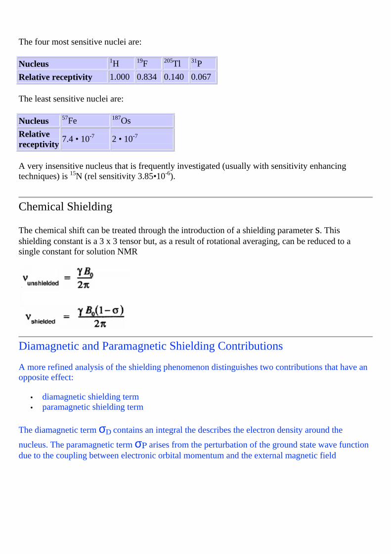
The diamagnetic term σD contains an integral the describes the electron density around the

nucleus. The paramagnetic term σP arises from the perturbation of the ground state wave function due to the coupling between electronic orbital momentum and the external magnetic field

The two equations should in principle allow the calculation of chemical shifts through quantum chemical methods but the quality of the results is at present rather variable.

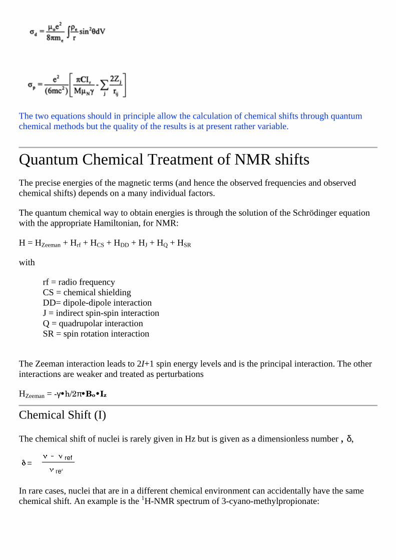
Quantum Chemical Treatment of NMR shifts

The precise energies of the magnetic terms (and hence the observed frequencies and observed chemical shifts) depends on a many individual factors.

The quantum chemical way to obtain energies is through the solution of the Schrödinger equation with the appropriate Hamiltonian, for NMR:

H = HZeeman + Hrf + HCS + HDD + HJ + HQ + HSR

with

rf = radio frequency CS = chemical shielding DD= dipole-dipole interaction J = indirect spin-spin interaction Q = quadrupolar interaction SR = spin rotation interaction

The Zeeman interaction leads to 2I+1 spin energy levels and is the principal interaction. The other interactions are weaker and treated as perturbations

HZeeman = -γ•h/2π•Bo•Iz

Chemical Shift (I)

The chemical shift of nuclei is rarely given in Hz but is given as a dimensionless number , δ,

In rare cases, nuclei that are in a different chemical environment can accidentally have the same chemical shift. An example is the 1H-NMR spectrum of 3-cyano-methylpropionate:

The close similarity in the chemical shifts of the two CH2 protons prevents us from seeing the expected coupling pattern (2 triplets). Instead, we see only a singlet. For details see the AB spin system below.

Chemical Shift: Aromatic Compounds

Aromatic compounds show a characteristic deshielding of ring protons (δ 6 - 9 ppm vs. δ 3 - 4 ppm for alkenes)

The explanation of this phenomenon relies on the analogy of aromatic rings with a closed conductor.

An external magnetic field induces a proportional current which in turn generates a (smaller) magnetic field whose direction is opposed to that of the external magnetic field on the outside of the conducting ring and parallel on the inside.

A particularly interesting case is the aromatic [14]Annulene and its antiaromatic dianion. The aromatic annulene shows strongly deshielded ring protons and strongly shielded endocyclic methyl groups. For the antiaromatic dianion, the situation is exactly reversed:

Polycyclic aromatic hydrocarbons show superpositions of different ring currents:

NMR Shift Reagents

Certain lanthanide compounds form complexes with molecules featuring -O- or -N< groups. Due to the magnetic moments of the paramagnetic lanthanide ions, this coordination leads to additional chemical shifts that decay with increasing distance to the metal ion.

The induced chemical shift depends on the distance between the paramagnetic atom (e.g. Eu) and the observed nucleus, but also on the angle between the two. The quantitative relation ship is the McConnell equation:

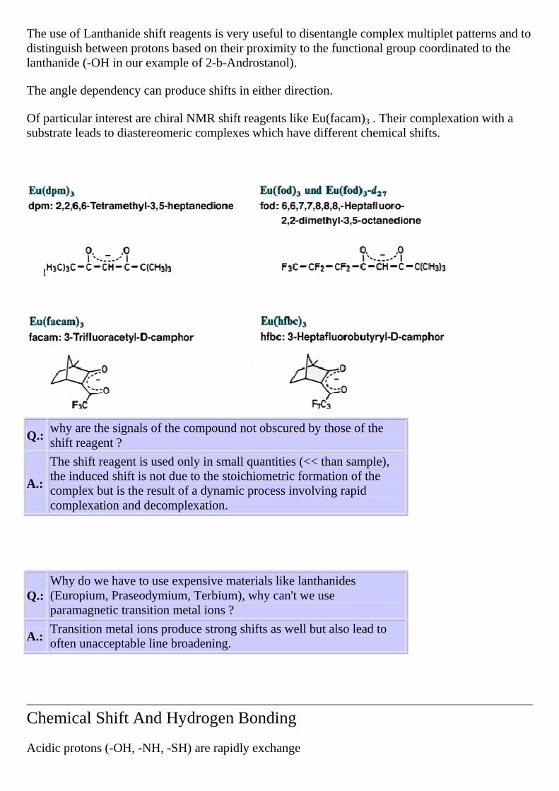
The use of Lanthanide shift reagents is very useful to disentangle complex multiplet patterns and to distinguish between protons based on their proximity to the functional group coordinated to the lanthanide (-OH in our example of 2-b-Androstanol).

The angle dependency can produce shifts in either direction.

Of particular interest are chiral NMR shift reagents like Eu(facam)3 . Their complexation with a substrate leads to diastereomeric complexes which have different chemical shifts.

Q.: why are the signals of the compound not obscured by those of the shift reagent ?

A.:

The shift reagent is used only in small quantities (<< than sample), the induced shift is not due to the stoichiometric formation of the complex but is the result of a dynamic process involving rapid complexation and decomplexation.

Q.: Why do we have to use expensive materials like lanthanides (Europium, Praseodymium, Terbium), why can't we use paramagnetic transition metal ions ?

A.: Transition metal ions produce strong shifts as well but also lead to often unacceptable line broadening.

Chemical Shift And Hydrogen Bonding

Acidic protons (-OH, -NH, -SH) are rapidly exchange

d through intermolecular hydrogen bonding. Two different shifts are involved in this exchange process, the shift of the free compound (1) and the shift of the hydrogen bonded species (2). Because the protons exchange rapidly between a and b, we only observe an averaged chemical shift.

For alcohols, the averaging involves the free alcohol ROH and the hydrogen bonded dimer (ROH)2 the relative amount of which is dependent on the concentration of the alcohol.

The chemical shift of the OH proton is therefore concentration dependent.

An important exception are compounds with intramolecular hydrogen bonding. Intramolecular hydrogen bonding (see salicylaldehyde below) is usually strong enough to suppress the exchange and we observe only on species with a shift that is largely independent of the concentration and temperature.

The 1H NMR spectrum below show a mixture of ethanol (intermolecular hydrogen bonding) and salicylaldehyde (intramolecular hydrogen bonding).

a) 5 % solution in CCl4 b) neat

Note the appearance of the ethanol-OH proton as triplet in the diluted sample (coupling to CH2) and absence in the neat sample (rapid exchange).

Spin-Spin Coupling

NMR active nuclei can couple with other NMR active nuclei that are in close proximity. This coupling leads to so called multiplets (doublet, triplet etc.). In solution, the predominant mechanism for spin-spin coupling is "through-bond". Coupling "through-space" usually suppressed by rapid rotation processes but can become important for rigid systems.

Spin-Spin coupling leads to the splitting of single lines into multiplets.

The number of lines in a multiplet (M) is determined by the number of identical coupling nuclei (n) and their nuclear spin I.

M = 2nI + 1

The overwhelming majority of multiplets are caused by the coupling of I - 1/2 nuclei which conveniently reduces the multiplicity formula to M = n + 1

The intensities of the individual lines is given by the spin I of the coupling nucleus (not the observed one). The relative intensities of the lines can be derived from Pascal's triangle and similar arrays:

Spin-Spin Coupling I > 1/2

A an example for a molecule with both I - 1/2 and I > 1/2 nuclei, we will now analyze the spin system of CH2D2,

The three types of NMR active nuclei (1H: I=1/2; 13C:I=1/2; 2D: I=1) lead to three different types of coupling constants:

2J (H,D)

1J (C,D)

1J (C,H)

In the proton NMR , we will only observe coupling to deuterium because the 13C atoms are not abundant enough (1.1 % natural isotopic abundance ) to be visisble under normal recording conditions.

In the carbon NMR, we have to consider the two different coupling constants

1J (C,D)

1J (C,H)

We know from the magnetogyric constants of 1H abd 2D that J(C,H) = 6.5 • J(C,D) in other words the C,H couling is much larger than the C,D coupling.

The 13C signal is therefore split into a large triplet by the presence of two protons.

Each of the three lines of this multiplet is then further split by the presence of two deuteriumatoms. The multiplicity is now (I = 1 for deuterium) (2 x 2 x 1) +1 = 5.

The overall splitting pattern is therfore a triplet of quintets.

The intensities of the individual lines of a multiplet depend of the nuclear spin I: For our case CH2D2, the line intensities of the quintet caused by the deuterium coupling are 1 : 2 : 3 : 2 : 1

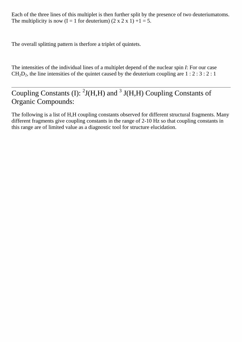
Coupling Constants (I): 2J(H,H) and 3 J(H,H) Coupling Constants of Organic Compounds:

The following is a list of H,H coupling constants observed for different structural fragments. Many different fragments give coupling constants in the range of 2-10 Hz so that coupling constants in this range are of limited value as a diagnostic tool for structure elucidation.

Coupling Constants: 1J(C,H)

The 1J(C,H) coupling constant can give valuable information about the structure of the molecule. The magnitude of 1J(C,H) is proportional to the s-character of the CH bond:

% s-character = 1J(C,H) / 500

The factor 500 is empirical and characteristic for Similar equations have been derived for many other combinations of elements. e.g.:

% s-character = -0.59 •1J(15N,H) -17.5

The validity of this relationship is readily verified by analyzing the coupling constants of methane (sp3), ethene (sp2) and ethine (sp).

The coupling constants of CHCl3 reflects the fact that the thc compound is CH-acidic. Chlorofrom is therfore often unsuitable as a solvent under conditions where CH2Cl2 is still inert.

Ring strain is partially compensated through a high p-character of the involved CC bonds. As a consequence, the exocyclic CH bonds possess a high s-character and show high 1J(C,H) coupling constants.

Coupling Constants (IX): Influence of Ring Strain on 3J(H,H)

Ring strain leads to changes in the hybridization (which ones ?) and this effects coupling constants:

Coupling Constants (V): 1J(C,C)

Due to the low natural abundance of 13C (the only NMR active isotope of carbon), it is very difficult to observe 13C-13C coupling. Only one out of 8000 molecules will possess two adjacent 13C isotopes. A method that uses the 1J(C,C) coupling to establish the C-C backbone of organic molecules is the INADEQUATE pulse sequence. INADEQUATE spectra are usually presented as 2D plots.

Like the 1J(C,H) coupling constant, the 1J(C,C) coupling constant depends on the hybridization (s-character) of the two carbon atoms Ca and Cb. A good approximation is:

1J(Ca,Cb) = 550 x %s(a) x %s(b)

Examples:

1) Ethane, 2 x sp3, => 1J(C,C) = 550 x 0.25 x 0.25 = 34 Hz (experimental: 35 Hz)

2) Ethylene, 2 x sp2, => 1J(C,C) = 550 x 0.33 x 0.33 = 60 Hz (experimental: 67.6 Hz)

Coupling Constants (VI): Quadrupolar Nuclei

Quadrupolar nuclei can in principle couple to I =1/2 nuclei like 1H, 31P , 13C, or 31P.

However, the linewidth of the quadrupolar nuclei is usually so broad that the coupling is hidden coupling. A comparison of the 14N and 15N NMR spectra of the tin complex below illustrates the point:

Coupling Constants (VIII): Cis-Trans Isomers of Olefins

The magnitude of the 3J(H,H) coupling constant in olefins follows the general rule Jtrans > Jcis and this is a convenient way to distinguish between cis and trans isomers:

3J is also influenced by the olefin's substituents, the distinction is meaningful only for one by direct comparison of the isomers or for olefins with very similar substitution pattern.

Coupling Constants (VI): Long Range Coupling

While 1J, 2J or 3J coupling is commonly observed for H,H coupling and 1J and 2J for C,H-coupling, coupling constants 4J or higher are usually too small to be observed.

A notable exception are 4J coupling constants in rigid frameworks, particularly those of "W-geometry."

Coupling Constants (VII): Heteronuclear Coupling

Most organic molecules contain 1H as only NMR active nucleus and observed couplings are accordingly those between neighboring protons.

The situation is more complex if other high abundance I = 1/2 nuclei are present. The only commonly encountered high abundance I - 1/2 nuclei are 19F and 31P.

The following spectrum is a 1H broadband decoupled 13C spectrum (shorthand notation: 13C {1H }) of trifluoroacetic acid that shows "hydrogen like " coupling (two quartets)

Quadrupolar nuclei can in principle couple to I=1/2 nuclei. The coupling is usually detectable by measuring the quadrupolar nucleus but rarely by measuring the I=1/2 nucleus (lifetime issue).

I =1/2 to I =1/2 is generally observed unless fast exchange disrupts the bond (loss of through-bond coupling)

14N NMR Spectrum of ammonium ions (a) and 199Hg NMR spectrum of di-tert-butylmercury (b); Spectrometer frequency 4.33 and 14.3 MHz. b: only 11 of the 19 expected lines are actually observed.

Coupling Constants (X): The Karplus Equation

The 3J(H,H) coupling constants of aliphatic H-C-C-H fragments depend on the dihedral angle.

The quantitative relationship is given by the Karplus equation.

The Karplus equation was first suggested by Martin Karplus and has become an extremely important tool for the elucidation of 3D structures through NMR methods. The

Applications of the Karplus Equation

Example: Sugars The Karplus equation is a useful tool to distinguish between the equatorial and axial protons present in many natural products. In the following example, the 3J(H,H) coupling constant s used to distinguish between a-D-Glucose and b-D-Glucose:

Example: Ethane. The Karplus equation can also be used to establish equilibrium constants in conformer mixtures. Ethane consist of a mixture of rotamers. The Karplus equation allows us to predict the 3J(H,H) coupling constant by assuming that all three staggered rotamers (t = 60o, 180o and 30o) are equally important:

Chemical and Magnetic Equivalence

It is usually fairly obvious which atoms in a compound are chemically equivalent. A precise definition would be

• chemically equivalent atoms are related by at least one symmetry operation

Chemically equivalent atoms also have identical chemical shifts and that might lead us to conclude that they are magnetically equivalent as well

However, this is not the case, magnetic equivalence is a more stringent criterion because we have to take into account the phenomenon of spin-spin coupling as well. Magnetically equivalent nuclei are:

• chemically equivalent (=possess the same chemical shifts) • have identical spin-spin interactions (=coupling constants) with other magnetic nuclei in the

molecule

This issue of identical vs. non-identical spin-spin interaction is best explained (and memorized) with the following 2 examples:

Difluoromethane has chemically equivalent protons and fluorine nuclei (mirror plane, C2-axis) which also have identical H-F coupling constants. The spin system is of the so called A2X2 type.

1,1-difluoroethylene has chemically equivalent pairs of hydrogen and fluorine atoms but there are now two different sets of coupling constants. The two hydrogens and fluorines are chemically equivalent (symmetry plane, C2 axis) but magnetically inequivalent they form a so called AA'XX' spin system. In view of the small number of nuclei involved, AA'XX' systems give rise to very complex spectra:

The magnetic inequivalence leads to the observation of two additional coupling constants: 2J(H,H') and 2J(F,F'). - Coupling between magnetically equivalent nuclei cannot be observed in the spectrum and this is why we do not see 2J(H,H) and 2J(F,F) in the example of difluoromethane.

The AB Spin System and Higher Order Spin Systems

If the two coupling nuclei have a very similar chemical shift, the intensity pattern of the individual lines deviates from that derived by the number pyramids. Such spin systems are labeled AB (AB2, A2B, A2B2 etc).

The intensity of the individual lines and hence the shape of the multipletsdepends on the ratio of the shift difference

(in Hz) νa - νb and the coupling constant J(A,B).

The hypothetical spectra of an AB systembelow illustrate this point:

a) J / (νa - νb) = 1: 3; b) J / (νa - νb) = 1: 1; c) J / (νa - νb) = 5: 3; d) J / (νa - νb) = 5: 1

Spectra like a) - d) which show deviations from the binomial intensity pattern are called higher order spectra.

Case d) can easily be mistaken for a singlet although it still is an AB system albeit without experimentally observed coupling constant. An example for this case is the 1H NMR spectrum of NC-CH2CH2-COOMe above.

Spectra with J / (νa - νb) > 1:10 have undistorted intensities and are called 1. order

spectra

AB Spin Systems

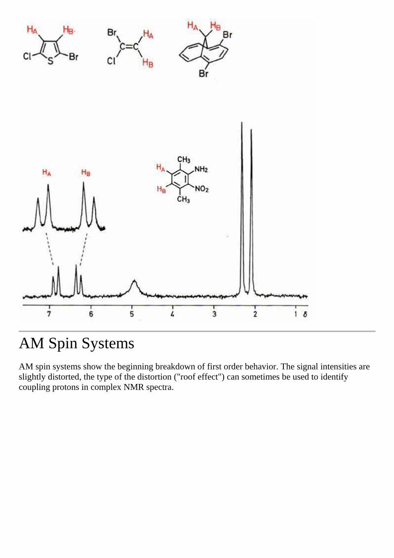
AM Spin Systems AM spin systems show the beginning breakdown of first order behavior. The signal intensities are slightly distorted, the type of the distortion ("roof effect") can sometimes be used to identify coupling protons in complex NMR spectra.

AA'BB' Spin Systems AA'BB' spin systems are higher order spins systems with complex but symmetric line patterns. A classical example for the AA'BB' spin system is ortho-Dichlorobenzene:

High resolution 1H NMR spectrum of o-dichlorobenzene (AA'BB' system) at 90 MHz.

AA'BB' spin systems are characterized by 4 independent coupling constants. Their determination is not readily obtained by visual inspection but best obtained through computer simulation.

AA'XX' Spin Systems The spin system of furan is similar to that of ortho-dichlorobenzene, but the chemical shifts of the ring protons are further apart which makes it AA'XX' spin system. The AA'XX' spin system has fewer lines but is deceptive in the sense that it resembles two triplets resulting from an A2X2 spin system (e. g. Cl-CH2-CH2-Br).

Lack of Coupling The absence of coupling can have a variety of reasons:

• magnetic equivalence, e.g. methyl protons H3C-R • no magnetic nucleus, e.g.. 1H-12C

• natural abundance too low, e.g. 1H-15N • coupling constant too small, e.g. 5J(H,X) • fast chemical exchange, e.g. H3C-OH • low lifetime of states (some quadrupolar nuclei, e.g. 35Cl, 79Br, 81Br, 127I)

Coupling to Low Abundance Spin 1/2 Nuclei: Satellite Signals Only a small number of NMR active nuclei occur with a natural abundance of 100 % (or close to 100%): 1H, 19F, 31P. Most NMR active nuclei have natural abundances in the range of 1- 20 %.

Spin 1/2 nuclei with intermediate natural abundance give rise to so called "satellites" with intensities reflecting the natural abundance of the isotope.

I = 1/2 elements that are readily detected in this way are:

Isotope Natural Abundance %

29Si 4.5 57Fe 2.2 77Se 7.6

107Ag - 109Ag

51.8 / 48.2

111Cd - 113Cd

12.7 / 12.3

117Sn - 119Sn

7.6 / 8.6

125Te 7.0 129Xe 26.4 171Yb 14.3 183W 14.4 187Os 1.6 195Pt 33.8

199Hg 16.8 203Tl / 205Tl

29.5 / 70.5

207Pb 22.6

The presence of satellites with the correct intensity is a valuable diagnostic tool to establish the presence of the respective element.

The spectrum above shows the proton decoupled 15N-NMR spectrum of a spirocyclic tin(IV) amide. All 4 nitrogen atoms are equivalent and couple to the central metal tin. The coupling to the two NMR active tin isotopes 117Sn and 119 Sn is well resolved.

The coupling constants for different isotopes A and B are usually differenttheir ratio is depends on

the magnetogyric ratios γA and γB:

J(A) / J(B) = γA / γB:

Using the γ-values for 117Sn and 119 Sn:

J( 117Sn) / J( 119Sn) = γ( 117Sn) / γ( 119Sn) = -9.578 / -10.021 = 0.956

The 117Sn and 119Sn satellites are usually well resolved like in the spectrum above and the appearance of double satellites is strong NMR evidence for the presence of tin in a given compound.

Selective Decoupling Individual nuclei can be "decoupled" if an external radio frequency exactly matches the Larmor frequency of the nucleus.

Decoupling experiments are usually carried out determine which of nuclei couple and which don't. The example of 3-amino-acroleine illustrates the technique.

• Selective irradiation of M reduces the AMX spin system to AX : two dublets, A-X coupling constant can be determined

• Selective irradiation of X reduces the AMX spin system to AM: two dublets, A-M coupling constant can be determined

Broadband Decoupling: 13C{1H}

All modern NMR spectrometers have the capability to decouple 1H. The most common use is to record broadband decoupled 13C NMR spectra. The shorthand notation is 13C{1H} with the curled brackets denoting the broadband decoupled nucleus.

The main application of broadband decoupling is the simplification of spectra. This is particularly valuable for 13C spectra that would otherwise consist of multiplets that tend to obscure each other by superposition.

The coupled (above) and 1H broadband decoupled (below) 13C-NMR spectra of the hydrocarbon norbornane illustrate this point:

While the triplet at ~ 30 ppm is readily identified with a CH2 group, the remaining multiplets obscure each other and are not readily recognized as what they are namely a triplet and a doublet.

The decoupled 13C NMR clearly shows the presence of three different carbon atoms

Coupling Constants of Different Isotopes

Although different isotopes of the same element have only very small differences in chemicals shifts, the coupling constants are often quite different. Coupling constants of different isotopes in the same compound are related through:

For the specific example H,D:

This means, that deuterium coupling constants are much smaller ( ~ 1/6.5) than the respective hydrogen coupling constants. It is therefore possible that X,H coupling produces the expected multiplet structure while the respective deuterated compound does not show the analogous multiplet resulting from X,D coupling because the coupling constant has become too small.

An example from our own research (M. K. Denk, J. Rodezno, J. Organometal. Chem. 2000 608 , 122-125 ) is the ring deuterated stable carbene below. The deuteration was observed when the stability of the carbene towards DMSO was investigated. Dissolution of a small amount of the carbene in DMSO-D6 (D3C-SO-CD3) produced the ring deuterated species.

While the ring protons showed a doublet of doublets with two well resolved coupling constants (1J(H,C) > 2J(H,C)), the smaller 2J(H,C) coupling constant remains unresolved in the deuterated compound (below, left). The IR spectrum of the deuterated compound (below, right) clearly shows the presence of a C-D bond, but the expected doublet (symmetric + antisymmetric combination) is not resolved.

Quadrupolar Nuclei

Quadrupolar Nuclei: Linewidths

Quadrupolar nuclei have an uneven charge distribution of the type shown below.

after R. K. Harris, "Nuclear Magnet Resonance Spectroscopy", Longman 1986, p132

While nuclei with I > 1/2 generally have shorter relaxation times and hence broader lines (lifetime broadening) the linewidth depends on the quadrupole moment of the nucleus and in particular on the symmetry of the environment.

Coupling With Quadrupolar Nuclei

The NMR properties of quadrupolar nuclei, in particular line width and coupling to other nuclei, crucially depend on the magnitude of the their quadrupole moment.

after R. K. Harris, "Nuclear Magnet Resonance Spectroscopy", Longman 1986, p136

Nuclei with small quadrupole moments like 2D (deuterium) and lithium 6Li have small quadrupole moments and resemble I = 1/2 nuclei in having small linewidths. They also couple with most I=1/2 nuclei. Typical quadrupolar nuclei like like 59Co show extremely broad lines and do not couple to other nuclei.

Quadrupolar Nuclei And Site Symmetry

The linewidth of quadrupolar nuclei depends not just on the magnitude of their respective quadrupole moment but also on how symmetric their environment is. A highly symmetric environment (tetrahedral, linear) leads to unusually small linewidths that can approach those observed for I = 1/2 nuclei.

The following table of 14N NMR data illustrates the point. Note the strong difference between [NMe4]

+ (tetrahedral) and :NMe3 (pyramidal).

after R. K. Harris, "Nuclear Magnet Resonance Spectroscopy", Longman 1986, p136

Symmetry and Coupling in Quadrupolar Nuclei

The following example of the 17O NMR spectrum of trimethylphosphate illustrates the importance of the relaxation time for the observation of coupling constants. While the the PO oxygen atom has a small line width that allows the easy detection of a 17O-31P coupling, the respective MeO signal is broad and the coupling to 31P is barely visible

Dynamic NMR (I): Coupling Constants and Chemical Exchange

Coupling may be lost if one of the coupling nuclei undergoes chemical exchange. A classical example is ethanol. In principle, we would expect that the proton of the OH group couples to the CH2 group and appears as a triplet. This is indeed observed but only in absolutely pure and dry ethanol.

The addition of water or traces of acid catalyze a rapid proton exchange between different ethanol molecules and the coupling to the OH proton is lost. Note that the CH3 group is unaffected (no coupling to OH).

In the presence of water, the OH signal o ethanol is not only "decoupled" but is also shifted towards the resonance of pure water. This is the result of a rapid proton exchange between water and ethanol.

Dynamic NMR (II): Measuring Activation Barriers through NMR

The rate of exchange of any reaction is described through the Eyring equation:

For the simples case of two singlets of equal intensity, the average frequency observed for a rapidly exchanging system will be:

In the intermediate temperature range between fast and slow exchange we will observe signals that begin to coalesce:

For a specific temperature, the average signal will begin to split. This temperature is the coalescence temperature Tc. The reaction rate at this temperature is:

inserting this value for k into the Eyring equation:

This is an equation that can be rearranged to give the free activation energy ∆G#at Tc:

(N = Avogadro number).

Or, after numerical solution with all constants for ν in Hz and T in Kelvin:

In other words, if we know the chemical shifts of two exchanging nuclei and the coalesence temperature, we can calculate DG#

Dynamic NMR (II): Hindered Rotation

A classical example for the unexpected observation of additional lines due to hindered rotation is dimethylformamide (DMF)

1H NMR Spectrum of dimethylformamide at room temperature (above 120 oC b/c coalesce to a single signal)

Dynamic NMR (III): Loss of Coupling In Floppy Rings

Chemical Shift (III): Chemical Exchange

Acetylacetone is a good example how a seemingly simple molecule can give rise to a fairly complex spectrum. We first have to note that acetylacetone is in equilibrium with its enol tautomer.

This equilibrium is slow on the NMR time scale so that two sets of signals for the two tautomers are observed in the 1H and 1H decoupled 13C NMR:

The enol can exist in two prototropic isomers but the energy barrier for their interconversion must be very low (or zero) because the two forms can not be observed separately.

(How would you modify acetylacetone so that the two enol isomers become distinguishable ?)

The Nuclear Overhauser Effect

The irradiation of an NMR active nucleus leads to distortions (usually: enhancements) in the intensity of neighboring nuclei. This can be signals that show very similar chemical shifts and would otherwise be difficult to distinguish:

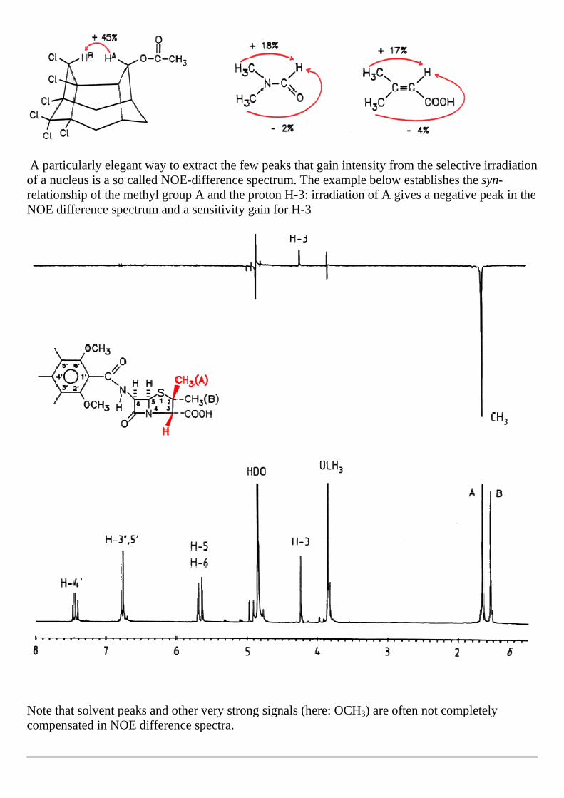
A particularly elegant way to extract the few peaks that gain intensity from the selective irradiation of a nucleus is a so called NOE-difference spectrum. The example below establishes the syn-relationship of the methyl group A and the proton H-3: irradiation of A gives a negative peak in the NOE difference spectrum and a sensitivity gain for H-3

Note that solvent peaks and other very strong signals (here: OCH3) are often not completely compensated in NOE difference spectra.

INEPT Measurements

INEPT was one of the first pulse sequences designed to boost the sensitivity of insensitive nuclei through NOE. The name stands for Insensitive Nuclei Enhancement by Polarization Transfer.

INEPT effects can also be used to assign signals.

The broadband decoupled 15N NMR spectrum (top) shows two nitrogen signals at roughly the same intensity. It was suspected that the slightly more intense signal at 359.6 ppm belongs to the CH2N nitrogen because this nitrogen has two a-protons exercising their NOE effect. An INEPT experiment with a typical 2J(1H,15N) confirms this assignment.

Signals from Noise: The Power of Fourier Transformation The classical way of measuring a spectrum is a frequency sweep, that is, we measure the intensity (absorbed, transmitted, reflected) for each frequency and slowly change the frequency. Recording times for individual spectra are then in the order of minutes.

A radically different approach is the simultaneous excitation of all frequencies. This leads to emission of a superposition of many individual frequencies corresponding to the individual absorption bands in other words: noise.

However, the emitted noise is not random but contains the frequency information of the individual spectral lines. The characteristic frequencies can be extracted through a mathematical process called Fourier Transformation .

"Robespierre fell from power on 27 July 1794, and Jean Baptiste Joseph Fourier, a diplomat and scientist who was to be executed the next day because of his involvement in revolutionary affairs 1, was spared. In 1807 Fourier was attempting to solve mathematically a problem concerning the conduction of heat by using a series expansion of sine and cosine terms that became familiar as Fourier Series.

The principles that Fourier established laid the foundation for mathematical methods of extraordinary power and flexibility that have not only stimulated continuing original contributions to pure mathematics, but have found a variety of applications in applied mathematics and science.

Fourier transformed NMR and IR Spectroscopy are now fully fledged analytical techniques that are used in laboratories throughout the world."

R. P. Wayne, "Fourier Transformed", Chem. Br. 1987, 440-445.

1) other then NMR, MD

The advantage is, the short noise bursts that follow the excitation are much faster to record than a frequency sweep. Moreover, many individual bursts (free induction decays = FIDs in NMR spectroscopy) can be accumulated in a computer and then transformed. It can be shown, that the S/N ratio increases with the number of accumulated spectra n as n1/2.

The following example shows the improvement of S/N for a series of accumulated (=superimposed) spectra:

after W. W. Paudler, Nuclear Magnetic Resonance, Wiley, 1987.

Pulse NMR

A simple way to explain the inner workings of pulse NMR is the vector formalism.

In the absence of an external magnetic field, the magnetic moments of the NMR active nuclei will be oriented at random. If we switch on the field, they will align to assume their allowed energy values. This alignment only implies a fixed z-component , mz, in x and y direction there is no quantiziation.

The vectors will thus lie on a cone:

The two different states m= + 1/2 and m= -1/2 have a slightly different population and this leads a net magnetization M 0 :

The Time Evolution of M

Relaxation describes, how the magnetization M0 of a sample returns to its thermodynamic equilibrium value (-> Boltzmann distribution). In the absence of an external field Bo, the spins are oriented at random. If we place the sample into an external field, the spins of the individual molecules will align.

This will build up magnetization along the z-axiz (M z) but will at the same time lead to a decay of the magnetization in the x,y plane (M x,y). The time evolution of these two processes is described by the Bloch equations with their two different time constants T1 and T2:

Integration gives the time dependence of M z :

The relationship says that the equilibrium (Boltzmann distribution) decays exponentially with time.

Detection of Polarization: The 90 o Pulse.

The transversal or spin-spin relaxation time T2 describes to the decrease of M y after a 90 degree pulse. The inhomogeneity of the magnetic field Bo ensures that the nuclear spins of different molecules have a slightly different Larmor frequency. This to a spreading of the individual magnetization vectors in the x,y plane and a net decrease of the the resulting total magtnetization M y over time.

The determination of T2 uses a pulse sequence that was proposed by Hahn.

Magnetic Resonance Imaging (MRI) and the value of T2-Relaxation

Magnetic resonance imaging relies on the high abundance of hydrogen (1H) in biological tissues. Most of the hydrogen is present in the form of water and that seriously limits our ability to differentiate between different types of tissues.

Fortunately, the relaxation times T2 of hydrogen in biological environments are slightly different and this difference in T2 is the basis for the contrast in MRI images. The sequence of eight MRI images shows 8 subsequent T2-echos. Note the decreasing luminosity (~ signal intensity) of the pictures.

The echos are generated with the Carr-Purcell-Maiboom-Gill pulse sequence. Time for one complete pulse sequence 0.3 seconds. Total measurement time 11 minutes. Bo = 1.5 Tesla.

The T2 values depend on the type of tissue and allow the rapid detection of tumors or other degenerative processes.

Relaxation Time T1

The relaxation times of individual nuclei determine the linewidth and (see below) the intensity of NMR signals. Apart from the chemical shift δδδδ and the coupling constant J, the relaxation time T is specific for a nucleus and its surrounding and can provide valuable chemical information.

1H shows only a small variation of T1 and is therefore rarely measured to gain chemical information.

13C shows a broad range of different relaxation times and 13C T1 and T1 measurements are increasingly used for structure elucidation purposes.

Relaxation Time T1 : Determination

T1 relaxation times are usually determined with the Inversion- Recovery Method.

The individual signals vanish at certain times tnull . T1 is obtained from tnull according to tnull = T1•ln2

From the tnul values of ethylbenzene above gave T1 times of 7.2 sec (CH3), and 72 sec (quaternary carbon).

T1-Relaxation Times of Carbon: Dipolar Coupling

The magnitude of T1 is determined by the neighborhood of dipolar nuclei (1H). This leads to the generally observed sequence of T1 times

CH3 < CH2 < CH < quaternary

The example of isooctane below illustrates this rule:

Isotopic substitution can lead to very selective changes of the T1 time. particularly valuable is the selective deuteration of compounds. Deuterium is a quadrupolar isotope and does not contribute towards the dipole-dipole relaxation. As a result, the relaxation times of carbon atoms increase in the proximity of deuterium atoms:

T1-Relaxation Times of Carbon: Molecular Motion

For linear molecules, the relaxation times of atoms towards the center of the long axis are significantly longer than those at the periphery of the molecules. The ends of long rigid molecules tend to relax faster than those of short molecules. This is nicely illustrated by the series Ph-Me, Ph-CCH, and Ph-Ph. The relaxation time of the para proton decreases with the length of the molecule from (15 seconds - 8.2 seconds - 3.2 seconds) and the same trend is observed for the ortho and meta protons. Extending the length of the molecule beyond biphenyl has little effect.

T1 relaxation times re uniquely suitable to distinguish individual carbon atoms in carbon chains. The first example shows the individual carbon atoms of decane, C10 H22. The left half of the molecule contains the full information due to the symmetry of the molecule.

Connection Between T2 and T2

• T2 is largely determined by field inhomogeneities DBo and does not contain much chemically useful information (see however MRI imaging above).

• T2 is an important parameter for multipulse experiments • T2 is measured through Hahn Spin-Echo experiments • T2 describes the time evolution of M x and M y (transversal magnetization) and is therefore

called transversal relaxation time. • T2 is largely driven by spin-spin interaction and is also called spin-spin relaxation for that

reason • The general rule is that T1 ³ T2 in other words the spins are often completely randomized in

the x,y plane before M z magnetization has reached thermal equilibrium. • T2 and T1 are of comparable magnitude for I=1/2 nuclei in solution and add up to give

natural linewidths of about o.1 Hz. • In solids, T1 is on the order of minutes or even hours (no tumbling !) but T2 becomes very

short (10-5 sec)) due to strong dipole-dipole interactions.

2D-NMR

Historic Development

2D Methods have greatly contributed to the explosive growth of NMR in the investigation of chemical and biological problems.

The first 2D-NMR experiment was reported by the Belgian Physicist Jeener. The most active developers of 2D methods were R. R. Ernst (Varian Research Center at Palo Alto and ETH Zürich) and R. Freemen (Oxford).

Types of 2D Experiments

2D methods can be broadly classified in shift-shift correlations (d,d methods) and those that display coupling constants and shifts (J,d methods). A 2D NMR spectrum displays signal intensity as the function of two frequency variables. An obvious advantage of the approach is the removal of signal crowding.

As an example, the resolving power of a 1H-13C HetCor experiment improves the resolving power by a factor of 1000 !

More important is the detection of spatial relationships between individual nuclei.

Measurement Time for Typical 2D NMR Experiments

2D-NMR: The Pulse Sequence

The appearance of 1D-spectra is determined by the three blocks of preparation, mixing and detection (=acquisition).

Preparation Mixing Detection (t2)

The pulse sequence of a 2D experiment adds a 4th block, the so called evolution time t1.

Preparation Evolution (t1) Mixing Detection (t2)

The detection period corresponds exactly to that of 1D experiments and the time t2 provides, after FT, the w2 axis of the spectrum.

The crucial difference that distinguishes the 2D methods is the introduction of a second, incrementally increased time, the so called evolution time t1. Separate FID's are collected for each incremental variation of t1. 2D-NMR uses a second Fourier Transformation that generates a second frequency axis w1 from t1.

While t2 is a "natural" time determined by the FID of the molecule, t1 can be manipulated to a wide degree.

The total number of increments is varied in exponents of 2 and is usually 128 or 256 although much lower numbers n are quite acceptable for some experiments.

2D-NMR: Description of Pulse Sequences

While It is possible to understand many 2D techniques as arrayed 1D pulse sequences 2D techniques involving phase correlation or multi quantum transition cannot be reduced to the 1D formalism.

A reasonably simple formalism to explain the results of 2D experiments in a qualitatively and quantitatively correct fashion is the so called product operator formalism. An excellent introduction to 2D-NMR with the product operator formalism is the famous Review by Kessler, Gehrke and Griesinger [H. Kessler, M. Gehrke and C. Griesinger, "Two-Dimensional NMR Spectroscopy: Background and Overview of Experiments" Angew. Chem. Int. Ed. Engl. 1988, 27, 490-536.]

2D-NMR: δ,J vs. δ,δ Experiments

The coordinate axis of a 2D NMR spectrum are invariably frequencies, but depending on whether these frequencies represent chemical shifts or coupling constants it is convenient to classify 2D

NMR in those that correlate shifts with shifts (d,d- experiments) and those that correlate shifts

with coupling (d,J- and d,D-experiments).

A third mechanism of information exchange is the chemical exchange of atoms. Exchange processes can be intermolecular or intramolecular.

2D-NMR: d,J vs. d,D Experiments

Both types of coupling, the scalar coupling (through bonds) and the dipolar coupling (through space) can be used for 2D methods. They are complementary to each other:

• 1J-coupling is used to establish the connectivity of covalent frameworks.

• 3J-coupling is sensitive to the dihedral angle and is used to establish conformations.

• D-coupling establishes the proximity of non-connected atoms through NOE transfer experiments

2D-NMR: Common Pulse Sequences

To make a selection which 2D pulse sequences are the most important to an inorganic chemist is a difficult task. Kessler's review states that in 1988 (!) more than 500 pulse sequences were known.

Most pulse sequences that were developed for organic molecules apply to organometallic molecules but many more are specific to fluxional problems not often encountered in organic chemistry and of course to the correlation of hetero-atoms like 1H-11B.

The following sections will discuss the most important 2D pulses:

• COSY • NOESY • EXSY • HMQC • INADEQUATE • Inverse Detection Techniques

COSY

A particularly popular 2D NMR experiment is the COSY experiment.

COSY experiments are often 1H-1H experiments but there are many other correlations in the literature.

The COSY transfer , which proceeds through J-coupling relies on quantum mechanical effects and

cannot be explained with classical models. By applying a single (p/2)x rf- mixing pulse, it is possible to transfer coherence of spin a into coherence of spin b where these spins couple. Only with coupling do off-diagonal peaks occur. Consequently, COSY spectra are a terrific way to establish connectivity of networks.

The (H,H) COSY experiment establishes the connectivity of a molecule by giving cross peaks (these are the off diagnonal peaks) for pairs of protons that are in close proximity. For the example of Glutamic acid below, we obtain cross peaks for the proton pairs (2,3) and (3,4). We do not observe a crosspeak for the pair (2,4), because these protons are not directly adjacent.

500 MHz (H,H) COSY Spectrum of Glutamic acid. 1-D spectra left and top. 10 mg of compound in 0.5 mL of D2O, 5 mm sample tube, 256 spectra, digital resolution of 2.639 Hz/data point. Total measurement time ca. 3h.

A relayed COSY experiment goes one step beyond a COSY experiment by showing cross peaks not just for pairs of adjacent protons, but for triples as well. As a result, we observe additional cross peaks like the one for the pair 2,4 in Glutamic acid below. Relayed COSY experiments can give cross peaks for protons that are too distant to show coupling in the 1D NMR spectrum.

500 MHz H-relayed (H,H) COSY Spectrum of Glutamic acid. 1-D spectra left and top. 10 mg of compound in 0.5 mL of D2O, 5 mm sample tube, 256 spectra, digital resolution of 2.639 Hz/data point. Total measurement time ca. 3h.

With present hardware and pulse sequences, it is possible to repeat the relay step up to three times. This allows the correlation of of protons that are separated by up to six bonds (d-protons). The relaying nucleus is typically 1H, but high abundance I =1/2 hetero-elements like 31P or 19F can be used as well.

2D-NOE Techniques

NOE techniques complement techniques that involve scalar coupling because they establish the proximity of non-bonded atoms. Most published data are on 1H,1H experiments. Common pulse sequences:

• NOESY (3-dimensional structure of molecules, exchange processes) • zz-NOESY (solvent peak suppression, differentiation between chemical exchange and NOE).

NOESY & HOESY

The cross peaks in NOESY are due to pairs of nuclei that are close enough (<2.5 Å) to have strong dipolar interactions. Moreover, the size of 1H-1H NOESY cross peaks is proportional to their distance. This is particularly valuable for the structure elucidation of proteins.

Heteronuclear NOESY experiments are sometimes called HOESY experiments.

EXSY

Cross peaks in EXSY spectra indicate pairs of nuclei that undergo rapid chemical exchange. EXSY and NOESY have essentially the same pulse sequence . Both require a mixing time to allow the random process of cross relaxation or exchange to occur.

The following 2D spectrum combines an EXSY spectrum (top-left) and a COSY spectrum (bottom-right) in one plot. The data show that only the carbonyl groups 6 and 7 undergo chemical exchange. Note that 6 from 7 lead two different peaks and are hence magnetically inequivalent.

Kinetic Data From EXSY

EXSY spectra can not only be used in a qualitative way to establish the absence or presence of chemical exchange. It is often possible to investigate the time constants of the exchange process by incremental variation of the acquisition parameters.

In the following example, the exchange of complexed and uncomplexed 7Li was studied by varying the mixing time of the 2D experiment. With 7 ms mixing time, the exchange process is barely visible while strong cross peaks are observed for a mixing time of 50 ms.

Limitations of COSY: Low Abundance I = 1/2 nuclei

In principle, the 13C-13C connectivity could be established through a C,C-COSY experiment, but the sensitivity of such a COSY experiment would reflect the natural abundance of a 13C-13C pairs (only one in 8000 molecules contributes to the experiment 0.01 times 0.01 = 10-4). If an HH-COSY experiment takes 1h, the respective CC-COSY would take 10,000 hours (more than a year) to achieve the same signal/noise ratio.

Conclusion: COSY is suitable only for abundant (ideally 100 %) nuclei like 1H, 31P or 19F. It must be noted that the COSY off-diagonal peaks can also become very weak for dilute spin nuclei and that 13C with only 1% natural abundance is an extreme case. Most other diluted I = 1/2 nuclei like 29Si, 15N, 119Sn or 183W are more abundant.

INADEQUATE: 13C-13C

13C-INADEQUATE experiments are the preferred substitute for a CC-COSY and is one of the most attractive pulse sequence for the structure determination of complex organic and organometallic structures. The experiment can be tuned in such a way that only 1J(13C,13C) coupling leads to cross peaks.

The INADEQUATE pulse sequence is still plagued by the very low abundance 13C-13C pairs, but it eliminates the very intense diagonal peaks which can to obscure cross peaks. Measurement times are ca 6 - 12 hours for concentrated samples (500 mg) on high field instruments.

The elimination of the diagonal peaks is due to the fact that the INADEQUATE pulse sequence is a so called double quantum coherence experiment. Because only those atoms that are directly connected give cross peaks it is usually very easy to map the carbon skeleton of a molecule. (See also N. Chr. Nielsen, H. Thøgersen

O. W. Sørensen "Doubling the sensitivity of INADEQUATE for Tracing out the Carbon Skeleton of Molecules by NMR" J. Am. Chem. Soc. 1995, 117, 11365-11366).