DEMOGRAPHY OF FERAL PIG POPULATIONS

AT FORT BENNING, GEORGIA

Except where reference is made to the work of others, the work described in this thesis is my own or was done in collaboration with my advisory committee. This thesis does not

include proprietary or classified information.

___________________________________ Laura B. Hanson

Certificate of Approval: ___________________________ ___________________________ James B. Grand Michael S. Mitchell, Chair Associate Professor Assistant Professor Forestry and Wildlife Sciences Forestry and Wildlife Sciences ___________________________ ___________________________ Stephen S. Ditchkoff Stephen F. McFarland Associate Professor Acting Dean Forestry and Wildlife Sciences Graduate School

DEMOGRAPHY OF FERAL PIG POPULATIONS

AT FORT BENNING, GEORGIA

Laura B. Hanson

A Thesis

Submitted to

the Graduate Faculty of

Auburn University

in Partial Fulfillment of the

Requirements for the

Degree of

Master of Science

Auburn, Alabama August 7, 2006

iii

DEMOGRAPHY OF FERAL PIG POPULATIONS

AT FORT BENNING, GEORGIA

Laura B. Hanson Permission is granted to Auburn University to make copies of this thesis at its discretion,

upon request of individuals or institutions at their expense. The author reserves all publication rights.

__________________________ Signature of Author

__________________________ Date of Graduation

iv

THESIS ABSTRACT

DEMOGRAPHY OF FERAL PIG POPULATIONS

AT FORT BENNING, GEORGIA

Laura B. Hanson

Master of Science, August 7, 2006 (B.S., University of California, Davis, 2001)

101 Typed Pages

Directed by Michael S. Mitchell

Feral pigs are an ecologically harmful invasive species that wildlife managers

have been unsuccessful at controlling. Understanding the demography and population

dynamics of a species is necessary to create successful management strategies because

the most effective way to reduce population growth is to target the vital rate which has

the largest potential to influence the population growth rate (λ). I estimated survival,

recruitment, λ, and the sensitivity of λ to changes in vital rates for a control population

and a treatment population, where a lethal removal management strategy was

implemented. I also created novel density estimation methods to address known biases in

closed capture-mark-recapture methods.

Reducing total survival via lethal removal was successful in reducing feral pig

population growth; however the most effective management strategy to reduce λ would

be to target juvenile survival. Density was difficult to estimate because feral pigs have

low and heterogeneous capture probabilities.

v

ACKNOWLEDGMENTS

Much thanks to the Mitchell “wet lab” for their support, assistance with critical

thinking, and quest to integrate good science with fun times. Thanks to my pig people:

Buck Jolley, Bill Sparklin, and Brian Williams for feral pig ecological discussions and

fieldwork assistance. J. Barry Grand and Nick Sharp provided data analysis assistance,

especially with Program MARK.

vi

Style manual or journal used: Journal of Applied Ecology Journal of Wildlife Management Computer software used: Microsoft Word (2003) Program MARK ver. 4.2 Program CAPTURE Microsoft Excel (2003) ArcView 3.2

vii

TABLE OF CONTENTS

LIST OF TABLES viii

LIST OF FIGURES x

THESIS INTRODUCTION 1

CHAPTER 1: EFFECT OF EXPERIMENTAL MANIPULATION ON DYNAMICS OF

FERAL PIG POPULATIONS

Abstract 3

Introduction 4

Methods 10

Results 19

Discussion 24

CHAPTER 2: NOVEL DENSITY ESTIMATION METHODS USING OPEN

MARK-RECAPTURE MODELS

Abstract 49

Introduction 50

Methods 54

Results 61

Discussion 65

THESIS CONCLUSION 75

CUMULATIVE BIBLIOGRAPHY 77

APPENDIX 1 86

APPENDIX 2 88

viii

LIST OF TABLES

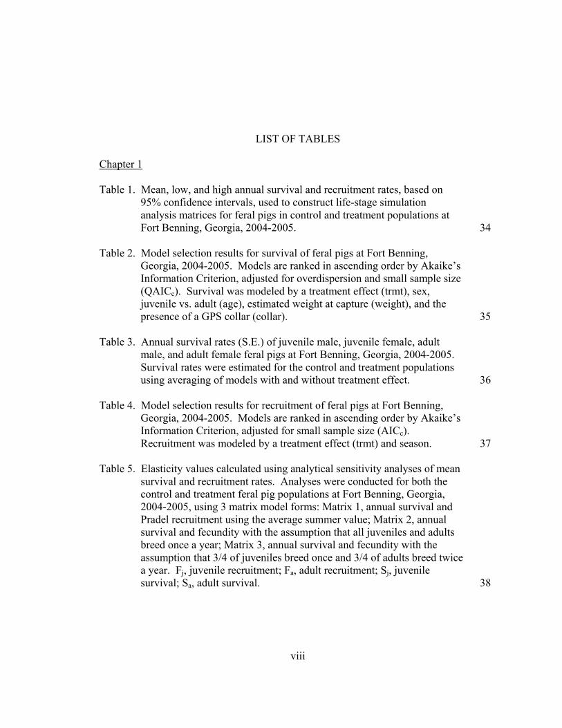
Chapter 1 Table 1. Mean, low, and high annual survival and recruitment rates, based on

95% confidence intervals, used to construct life-stage simulation analysis matrices for feral pigs in control and treatment populations at Fort Benning, Georgia, 2004-2005. 34

Table 2. Model selection results for survival of feral pigs at Fort Benning,

Georgia, 2004-2005. Models are ranked in ascending order by Akaike’s Information Criterion, adjusted for overdispersion and small sample size (QAICc). Survival was modeled by a treatment effect (trmt), sex, juvenile vs. adult (age), estimated weight at capture (weight), and the presence of a GPS collar (collar). 35

Table 3. Annual survival rates (S.E.) of juvenile male, juvenile female, adult

male, and adult female feral pigs at Fort Benning, Georgia, 2004-2005. Survival rates were estimated for the control and treatment populations using averaging of models with and without treatment effect. 36

Table 4. Model selection results for recruitment of feral pigs at Fort Benning,

Georgia, 2004-2005. Models are ranked in ascending order by Akaike’s Information Criterion, adjusted for small sample size (AICc). Recruitment was modeled by a treatment effect (trmt) and season. 37

Table 5. Elasticity values calculated using analytical sensitivity analyses of mean

survival and recruitment rates. Analyses were conducted for both the control and treatment feral pig populations at Fort Benning, Georgia, 2004-2005, using 3 matrix model forms: Matrix 1, annual survival and Pradel recruitment using the average summer value; Matrix 2, annual survival and fecundity with the assumption that all juveniles and adults breed once a year; Matrix 3, annual survival and fecundity with the assumption that 3/4 of juveniles breed once and 3/4 of adults breed twice a year. Fj, juvenile recruitment; Fa, adult recruitment; Sj, juvenile survival; Sa, adult survival. 38

ix

Table 6. Comparison of relative vital rate elasticities to relative LTRE contributions using average summer recruitment rates for control and treatment populations of feral pigs at Fort Benning, Georgia, 2004-2005. Fj, juvenile recruitment; Fa, adult recruitment; Sj, juvenile survival; Sa, adult survival. 39

Chapter 2 Table 1. Model selection results for abundance of feral pigs at Fort Benning,

Georgia, 2004-2005 using program MARK. Models are ranked in ascending order by Akaike’s Information Criterion, adjusted for small sample size (AICc). Capture (p) and re-capture (c) probabilities were modeled by year, sex, age, estimated weight, and rainfall presence on the day of capture (rain). 71

x

LIST OF FIGURES

Chapter 1 Figure 1. Map of the 737 km² Fort Benning Military Reservation in west-central

Georgia, site of the experimental feral pig study, showing the control and treatment study areas. 41

Figure 2. Basic life cycle for feral pigs with juvenile and adult age classes. F

represents fecundity or recruitment and S represents survival corresponding to the population matrix models. 42

Figure 3. Seasonal survival and recruitment rates estimated for female feral pigs

in control and treatment populations for each 4 month season (summer, fall/winter, and spring) at Fort Benning, Georgia, 2004-2005. Squares, survival rate; triangles, recruitment rate; closed symbols, control population; open symbols, treatment population. 43

Figure 4. Annual population growth rates and 95% confidence intervals for feral

pigs in control and treatment populations at Fort Benning, Georgia, 2004-2005, calculated using the following matrix model forms: Matrix 1, annual survival and Pradel recruitment; Matrix 2, annual survival and fecundity with the assumption that all juveniles and adults breed once a year; Matrix 3, annual survival and fecundity with the assumption that 3/4 of juveniles breed once and 3/4 of adults breed twice a year. Closed symbols, control; open symbols, treatment; circles, matrix using recruitment; squares, matrix using fecundity. 44

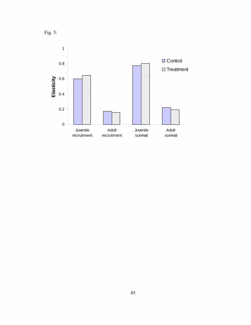
Figure 5. Analytical elasticities of juvenile recruitment, juvenile survival, adult

recruitment, and adult survival for control and treatment feral pig population at Fort Benning, Georgia, 2004-2005, calculated using the matrix incorporating annual female survival rates and annual Pradel recruitment rates. 45

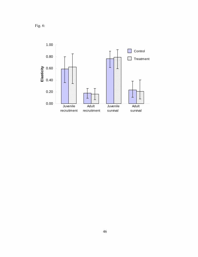
Figure 6. Life-stage simulation analysis elasticity values and 95% confidence

intervals of juvenile recruitment, adult recruitment, juvenile survival, and adult survival for feral pigs in control and treatment populations at Fort Benning, Georgia, 2004-2005. 46

xi

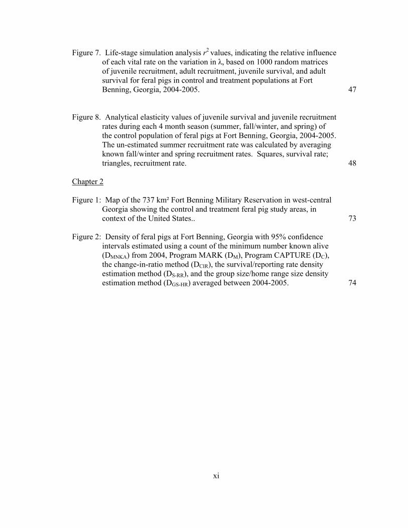
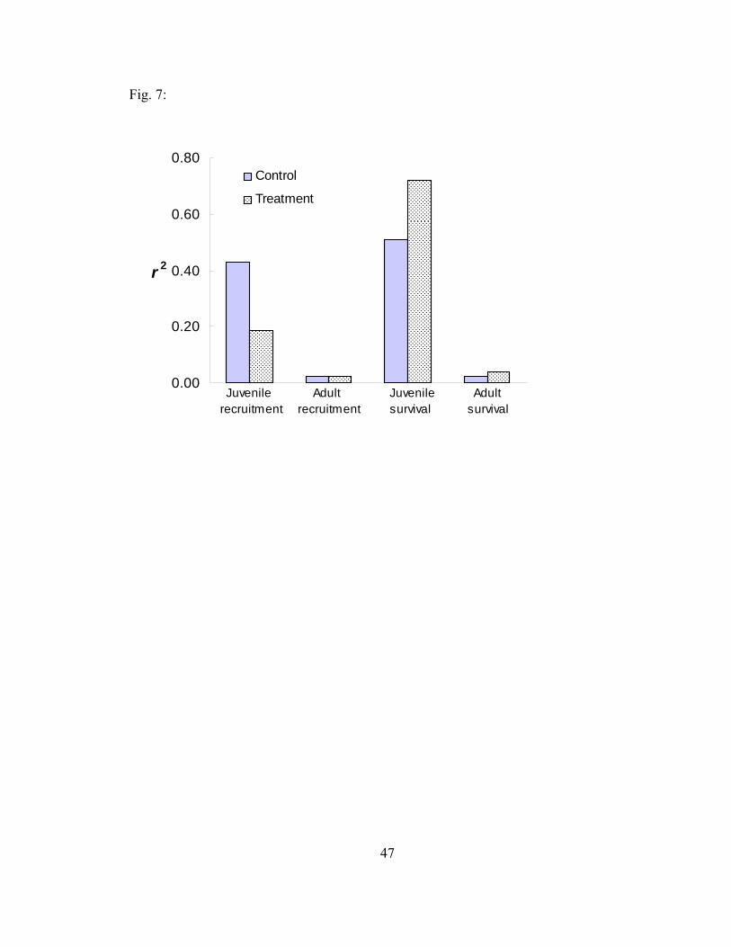
Figure 7. Life-stage simulation analysis r2 values, indicating the relative influence of each vital rate on the variation in λ, based on 1000 random matrices of juvenile recruitment, adult recruitment, juvenile survival, and adult survival for feral pigs in control and treatment populations at Fort Benning, Georgia, 2004-2005. 47

Figure 8. Analytical elasticity values of juvenile survival and juvenile recruitment

rates during each 4 month season (summer, fall/winter, and spring) of the control population of feral pigs at Fort Benning, Georgia, 2004-2005. The un-estimated summer recruitment rate was calculated by averaging known fall/winter and spring recruitment rates. Squares, survival rate; triangles, recruitment rate. 48

Chapter 2 Figure 1: Map of the 737 km² Fort Benning Military Reservation in west-central

Georgia showing the control and treatment feral pig study areas, in context of the United States.. 73

Figure 2: Density of feral pigs at Fort Benning, Georgia with 95% confidence

intervals estimated using a count of the minimum number known alive (DMNKA) from 2004, Program MARK (DM), Program CAPTURE (DC), the change-in-ratio method (DCIR), the survival/reporting rate density estimation method (DS-RR), and the group size/home range size density estimation method (DGS-HR) averaged between 2004-2005. 74

1

INTRODUCTION

This thesis describes the demography and population dynamics of feral pigs (Sus

scrofa) at Fort Benning, Georgia. This research was conducted to determine the

population size, survival rates, recruitment rates, population growth rates (λ), and the

sensitivity of λ to changes in age-specific vital rates of feral pigs at Fort Benning,

Georgia in order to determine the most effective method to reduce feral pig population

growth rates.

Feral pigs are an ecologically harmful invasive species with expanding

distributions in many parts of the world. Within the southeastern United States, Fort

Benning personnel are concerned about the effects of feral pigs on threatened and

endangered species and ecosystem functions. Because of their range expansion, habitat

use, and potential for spreading disease, many wildlife managers, including those at Fort

Benning, are interested in reducing feral pig population sizes and λ.

In order to develop an effective management plan, feral pig demography,

including density, survival, recruitment, and λ, must be understood because the most

effective way to reduce λ is to target the vital rate, which has the largest potential to

influence λ. Density can be used to determine the intensity of management required to

reduce the population size and to monitor the effects of a management strategy over time.

I developed novel density estimation methods to address biases associated with

2

estimating population sizes for wildlife species, such as feral pigs, with low or

heterogeneous probabilities of being captured.

Creating effective management plans requires not only understanding the

demography of a species, but also how a particular management strategy affects various

aspects of the demography. To understand how a lethal removal management strategy

affects the vital rates and the influence of those vital rates on λ, I compared demography

and vital rate sensitivity of a non-manipulated control population to that of a manipulated

treatment population, where I conducted lethal removal of feral pigs via trapping and

shooting. I conducted an experimental manipulation to more fully understand how lethal

removal affects the population dynamics of feral pigs and to create an effective feral pig

population reduction strategy. I also used the experimental manipulation to examine the

possibility of a density dependent response in feral pig recruitment rates.

3

EFFECT OF EXPERIMENTAL MANIPULATION ON DYNAMICS OF

FERAL PIG POPULATIONS

Abstract

1. Invasive species, such as feral pigs (Sus scrofa) are often ecologically harmful

and have expanding distributions. Effectively reducing feral pig populations,

which is becoming an increasingly common objective of wildlife managers,

requires determining how reduction efforts affect vital rates and which vital rate

potentially has the largest effect on the population growth rate (λ).

2. We implemented a manipulative experiment of feral pig populations at Fort

Benning, Georgia to assess the demographic effects of a lethal reduction. We

compared demography of a non-manipulated control population with a treatment

population, where feral pigs were experimentally removed. Using mark-recapture

data from trapping, re-sight with cameras, telemetry of radio-collared pigs, and

hunter-returned tags, we estimated survival, recruitment, and population growth

rates of treatment and control populations for 2004-2005. Matrix model

analytical and simulation sensitivity analyses were used to determine which

seasonal vital rate could potentially contribute most to changes in the population

growth rate.

4

3. The top ranked model for survival included a treatment effect; survival was lower

for the treatment population compared to that for the control. Recruitment

estimates did not differ between treatment and control populations, but the

population growth rate was lower for the treatment population compared to that

for the control.

4. Both analytical and simulation sensitivity analyses indicated that the population

growth rate was potentially most sensitive to changes in juvenile survival,

especially during fall/winter and summer. Simulation sensitivity analysis

revealed that the sensitivity of λ to juvenile survival increased as survival

decreased in the treatment population.

5. Based on our lethal removal efforts, reducing survival can be used in management

to lower population growth rates of feral pigs. However, management actions

lowering juvenile survival or juvenile recruitment will most effectively lower the

growth rate of feral pig populations and ultimately reduce the adverse effects of

feral pigs on native species.

Key-words: elasticity, mark-recapture, matrix model, population growth rate,

recruitment, sensitivity analysis, survival, Sus scrofa

Introduction

Management of invasive species is becoming increasingly important for

protecting native species and ecosystem functions (Townsend 2003, Batten et al. 2006).

Modeling population dynamics with the use of demographic data aids in understanding

5

what drives persistence and expansion of invasive species populations in their introduced

range. Population matrix models are often used to develop management strategies for

controlling invasive species (Citta and Mills 1999, McEvoy and Coombs 1999, Shea and

Kelly 1998).

Feral pigs (Sus scrofa) are an invasive species with expanding populations in

North America, Australia, and New Zealand (Clarke and Dzieciolowski 1991, Hone

2002, Mayer and Brisbin 1991). Feral pigs are considered economic and environmental

pests due to their effect on ecological processes by competing with native wildlife for

food resources (Dickson 2001), disturbing soil and vegetation while rooting for food

(Hone 2002), reducing species richness in plant communities (Kotanen 1995), and

occupying areas with sensitive animal species (MacFarland et al. 1974).

Lethal removal efforts are commonly used to attain short-term reductions in

population density to reduce detrimental effects of feral pigs (Hone and Pedersen 1980,

Engeman et al. 2001), but rarely have long-term density reductions or eradications been

achieved (Singer 1981, Izac and O’Brien 1991, but see Katahira et al. 1993). A model

constructed from demographic data on a feral pig population in New Zealand predicted

that a population reduced by 95% would recover to its original size in less than five years

(Dzieciolowski et al. 1992), demonstrating the potential difficulty in controlling feral pig

populations. While lethal removal is frequently used in feral pig management, little is

known about its effects on population growth rates (λ) and other vital rates (e.g., survival,

recruitment, etc.).

Development of an effective management approach for invasive species requires

accurate estimates of population vital rates and an evaluation of how removal affects

6

them. Vital rates of feral pig populations need to be understood because the most

effective way to reduce λ is to target the vital rate that has the greatest potential to

influence λ. Currently, the effect of management on the potential influence of each vital

rate is unknown. Species with long life spans and low reproductive rates often have

population growth rates which are most influenced by changes in adult survival (Heppell

et al. 2000). However, feral pigs are unlike most large mammals in that they have an

early age of maturity and high reproductive rates indicating that λ could be most

influenced by changes in recruitment.

The objectives of my research were to examine the demography of feral pig

populations and determine the demographic effects of an experimental population

manipulation using lethal removal methods. To accomplish these goals, I first estimated

survival and recruitment rates of treatment (lethal removal) and un-manipulated control

populations using maximum likelihood mark-recapture methods (Williams et al. 2002). I

used the vital rate estimates and population matrices to calculate λ and to evaluate the

effectiveness of the lethal removal efforts. To determine the potentially most influential

vital rate on λ, which is necessary for developing effective management strategies to

reduce λ, I conducted analytical and simulation sensitivity analyses (Caswell 2001,

Wisdom et al. 2000). To understand how each vital rate actually contributed to λ, I

conducted life table response experiments (LTRE) and examined seniority parameters.

Finally, to assess possible demographic density dependence, I compared vital rates and λ

from both control and treatment populations.

Survival and recruitment rates can be accurately estimated using mark-recapture

methods, which incorporate detection probabilities (Williams et al. 2002). The few

7

studies that have estimated survival rates for feral pigs used only age structure data or

radio-telemetry of a few individuals (Gabor et al. 1999, Saunders 1993). The Barker

mark-recapture model produces relatively robust estimates of apparent survival because it

provides a way to incorporate mark-recapture data, live re-sight, and dead recovery data,

which greatly increases the precision of the parameter estimates (Barker 1997).

No studies have been published documenting recruitment (i.e., the rate at which

individuals are added to the population through births and immigration) of feral pigs, but

data on fecundity (i.e., litter size or number of young produced per female per year) is

abundant. Female feral pigs can become sexually mature by five months old, an early

age compared to mammals with similar body mass (Read and Harvey 1989,

Dzieciolowski et al. 1992). Adult females often breed seasonally two times a year, but

can breed up to three times in a 14 month period (Coblentz and Baber 1987,

Dzieciolowski et al. 1992). Females produce approximately 5-7 piglets per litter (Taylor

et al. 1998), but can produce as many as 11 (McIlroy 1990). Although much is known

about feral pig fecundity, these data do not include estimates of immigration, which can

also affect λ. The Pradel reverse-time model uses mark-recapture data to estimate

recruitment rates by inverting capture histories to estimate seniority, the probability an

individual caught at time t was present in the population at time t-1 (Pradel 1996).

Population matrix models incorporate survival and recruitment rates to estimate λ.

I used matrix models to calculate the sensitivity of λ to changes in vital rates and the

relative contribution of each vital rate to λ (Caswell 2001). The use of recruitment rates

in matrix models instead of the traditionally used fecundity estimates should more

accurately estimate λ and vital rate sensitivity by including the potential contribution of

8

immigration to λ. Analytical sensitivity analysis is a useful tool to examine how relative

changes in mean vital rates potentially affect λ. Life-stage simulation analysis (LSA)

takes into account variation and uncertainty in vital rates in order to address the influence

of large, simultaneous, and disproportionate changes in vital rates on the variation in λ

(Wisdom et al. 2000). In contrast, LTRE is an extension of analytical sensitivity analysis

that takes into account observed changes in vital rates and vital rate sensitivity to

determine which vital rate actually contributed most to λ over a period of observation.

The seniority parameter, estimated to derive recruitment in the Pradel mark-recapture

model, can also be used to calculate the contributions of survival and recruitment to λ

(Nichols et al. 2000). Using multiple techniques to answer the same question strengthens

support for conclusions when the results are similar and highlights uncertainty when

results differ. The comparison of vital rate sensitivity analyses to actual vital rate

contributions can elucidate which vital rate is most important to population growth as

well as the demographic mechanisms for population change (Wisdom et al. 2000).

For environments with seasonal variation in food resources or hunting pressure,

the use of seasonal matrix models is valuable for examining differences in vital rate

sensitivity by season. Recruitment rates of feral pigs may vary seasonally with

differences in the availability of food resources. Seasonal mast crops, such as acorns, are

known to be important for body condition (Matschke 1967a), which is positively

correlated with reproductive performance (Gaillard et al. 1993). Survival may vary

seasonally as hunting pressure changes throughout the year. Sensitivity analyses of

seasonal matrix models will provide insights into how survival, recruitment, and the

effectiveness of different management techniques might vary by season.

9

Demographic density dependence has been shown in many wildlife populations

with survival and recruitment rates varying at different population densities (Rotella et al.

1996, Portier et al. 1998). In general, λ increases as population density decreases for

most animal populations (Tanner 1966), but the exact relationship between density and λ

is rarely known. Although understanding how vital rates change at different densities has

strong management implications, Sibly and Hone (2002) identified only 25 studies in the

literature that plotted λ against population density. In the case of invasive species,

wildlife managers are concerned about density dependence acting to limit the

effectiveness of management efforts as animals compensate by increasing survival or

recruitment at lower densities. Examination of vital rates and population growth rates

within a species can lead to increased knowledge of how and when density dependence

operates.

I studied feral pig populations at Fort Benning, Georgia, to examine four

alternative hypotheses describing the sensitivity of λ to changes in vital rates. I

hypothesized that λ was potentially most sensitive to changes in juvenile recruitment,

adult recruitment, juvenile survival, or adult survival. I examined the effect of

experimental manipulation on the sensitivity of each vital rate.

I also evaluated two hypotheses regarding density dependence. I hypothesized

that if the feral pig population at Fort Benning demonstrated density dependence such

that experimental removal did not reduce λ because the population exhibited

demographic density dependence, then I predicted A) recruitment rates would be greater

in the treatment population than the control population as the remaining females in the

treatment area increased their reproductive output or as pigs immigrated into the

10

treatment area and B) juvenile survival would be greater in the treatment population than

the control population. If either of the predictions were supported, the population would

be considered density dependent, but if both predictions were shown to be false, it would

be considered density independent.

Methods

STUDY AREA

My research was conducted between spring 2004 and fall 2005 at the Fort

Benning Military Reservation in west-central Georgia (32°21’N, 84°58’W). The 737

km² military base is located on the Coastal Plain-Piedmont Fall Line with elevations

ranging from approximately 50 to 230 m. The climate is semi-tropical with an average

annual rainfall of 132 cm (Dilustro et al. 2002). The average maximum temperatures in

July and January are 33.2° C and 13.8° C, respectively. Fort Benning is primarily

dominated by stands of longleaf pine (Pinus palustris), loblolly pine (P. taeda), shortleaf

pine (P. echinata), and scrub oak species (Quercus spp.) in the uplands. The understory

is generally open with some shrubs and grasses. The riparian bottomlands consist of

yellow poplar (Liriodendron tulipifera), sweet gum (Liquidambar styraciflua), red maple

(Acer rubrum), hickory (Carya spp.), ash (Fraxinus spp.), and oak species (King et al.

1998).

EXPERIMENTAL DESIGN

To determine the effects of experimental removal on population demography, I

compared a non-manipulated control population with a treatment population. I

11

considered the 50 km² control and treatment areas, located approximately 8 km apart and

separated by a large creek, independent study sites (Fig. 1). I caught, tagged, and

released feral pigs in both the control and treatment populations during summer 2004

(May –July), before I began the experimental removal. The experimental removal

consisted of killing feral pigs via lethal trapping and shooting in the treatment study area

from August 2004 through May 2005. Lethal trapping involved shooting pigs captured in

spring-loaded cage traps baited with corn. I estimated survival, recruitment, and λ from

summer 2004 to summer 2005 of feral pigs in both control and treatment populations.

During the summer of 2005, I repeated the mark-recapture of pigs in both control and

treatment areas. Hunting by off-duty military personnel occurred year-round in both

study areas.

TRAPPING AND HANDLING

I conducted capture-mark-recapture sessions during each summer, 2004 and 2005.

I spaced 20 trap locations 1-2 km apart across each study area. I pre-baited traps with

shelled corn and corn mash for two weeks prior to each trapping session. I trapped feral

pigs in cage traps capable of catching multiple pigs. I checked traps each morning of the

18 day trapping sessions.

I tagged all captured feral pigs with uniquely numbered ear tags in both ears using

yellow and white tags to indicate study area (National Band and Tag, Newport, KY). I

measured head and body length in order to estimate age (Boreham 1981). I recorded sex

and estimated weight prior to release. I used Telazol (1 cc/ 30 kg), administered with a

jab stick, to sedate adult females and attach ear tags and a GPS collar (Advanced

12

Telemetry Systems, Isanti, MN). I recorded body measurements of each sedated female

and aged them based on tooth eruption patterns (Matschke 1967b). I monitored GPS-

collared feral pigs via radio-telemetry weekly to determine potential mortality. Handling

and removal of all pigs was conducted in accordance with institutional animal care and

use guidelines of Auburn University (# 2003-0531).

CAMERAS

I used digital game cameras (infrared Digital-Scout 3.2 megapixel; Penn’s

Woods, Export, Pennsylvania, USA) to re-sight ear tagged and other individually

identifiable feral pigs passively in both study areas between August 2004 – May 2005. I

baited 16 cameras with fermented corn and moved them every 2 to 3 weeks in order to

fully sample the study area several times. I set cameras with a 2 minute delay between

photographs being taken to acquire multiple photographs of the same feral pig group to

assist with identification. I photographed each feral pig before its initial release to aid in

identifying tagged feral pigs re-sighted with the game cameras. I identified untagged

feral pigs by unique pelage markings.

SURVIVAL

To estimate survival using a maximum likelihood method, I used the capture-

mark-recapture Barker model in program MARK (White and Burnham 1999, Barker

1997). I included data on live trapping, “re-sight” of GPS collared feral pigs via radio-

telemetry, camera re-sight, and hunter returns of ear tags to estimate apparent survival

and a reporting parameter (r), the probability of a tag being reported given that the

13

individual was found dead. This model also estimates capture probability (p), re-sight

probability (R), probability the animal is re-sighted and then dies within the interval (R’),

probability of fidelity to study area (F), and probability of temporary emigration from

study area (F’), all of which I considered nuisance parameters, i.e., parameters that must

be estimated in order to estimate survival. I simplified models by holding nuisance

parameters constant over time and space because survival was the primary parameter of

interest and I had limited data. I modeled the reporting parameter by study area because I

reported most (93%) of the dead ear tagged feral pigs in the treatment area, whereas only

hunters reported dead feral pigs in the control area. Because the size of my dataset

prevented me from estimating movement parameters, I assumed random emigration by

constraining F = F ’= 1. I modeled survival using individual covariates including

treatment effect, sex, age, estimated weight, and presence of a GPS-collar.

I based model selection on the information-theoretic approach (Burnham and

Anderson 2002). I used Akaike’s Information Criterion (AICc) corrected for small

sample sizes to rank models (Akaike 1973).

Before running my a priori candidate model set, I constructed the most highly

parameterized, biologically relevant model for which all parameters could be estimated. I

used this global model to run a goodness-of-fit test to evaluate overdispersion in my data.

I assessed goodness-of-fit using a median ĉ test available in program MARK (White and

Cooch 2005). If data are not overdispersed, ĉ = 1. Any values of ĉ > 1 indicate lack of

fit. I incorporated the estimated ĉ value into the AIC calculation. I calculated odds ratios

by exponentiating the slope estimate from the logit link of the survival models.

14

Program MARK uses capture histories created for each individual feral pig to

estimate survival. I considered pigs less than 8 months old to be juveniles based on the

youngest age of first reproduction (Dzieciolowski et al. 1992, B. Jolley unpublished

data). Because feral pigs less than one month old were too small to be caught in traps,

estimates of juvenile survival included only feral pigs between 1-8 months old. I

estimated both annual and seasonal survival rates. I divided the year into three equal 4

month long seasons: summer (June – September), fall/winter (October – January), and

spring (February – May). Summer months are associated with lower food availability

compared to fall/winter with mast crops and spring with new vegetative growth.

Fall/winter months also correspond with deer hunting season. I estimated annual

variance using total variance because process variance could not be isolated (Seber

1982).

I estimated the mean lifespan of feral pigs at Fort Benning using the average

survival rate for all age and sex classes as well as for all females from the non-

manipulated control population. Mean lifespan = -1/ln(survival rate) (Brownie et al.

1985).

RECRUITMENT

I modeled recruitment using the maximum likelihood capture-mark-recapture

approach by Pradel in Program MARK (Pradel 1996). The Pradel model directly

estimates 3 parameters: survival probability, capture probability, and seniority

probability. The Pradel parameterization uses the seniority probability (γ), the

probability that an individual was present in the population at the previous time step and

15

is the equivalent of reverse-time survival, to estimate a per capita recruitment rate, which

includes reproduction, immigration, emigration, and juvenile survival. The seniority

parameter can also be used to examine contributions of survival and recruitment to λ

(Nichols et al. 2000).

I created capture histories for ear tagged and uniquely identifiable individuals

using only camera sight and re-sight data to reduce heterogeneity that can be caused by

including other capture methods. I modeled recruitment solely by treatment and season

because I lacked measurable covariates from un-tagged individuals. I estimated seasonal

recruitment rates for both control and treatment populations, but lack of data prevented

estimation of summer recruitment rates. To approximate summer recruitment, I created a

range of probable recruitment rates by using the rates from other seasons to get low,

average, and high summer rates.

I estimated fecundity by calculating average litter size in reproductive tracts

collected from harvested feral pigs. I divided pregnant sows into two groups, first time

breeders (≤ 1 year) and non-first time breeders (> 1 year old), to examine a potential litter

size difference between juveniles and adults.

To examine possible density dependence in recruitment, I compared λ estimates

for the control and treatment populations to recruitment estimates.

POPULATION MODELS AND SENSITIVITY ANALYSES

To examine λ, sensitivity, and elasticity in both annual and seasonal contexts, I

created 3 different types of post-birth pulse age-based population matrices modeling only

the female portion of the population based on the life-cycle of feral pigs (Fig. 2). I

16

created matrices populated with recruitment estimates and fecundity estimates to compare

λ estimates and vital rate sensitivity. First, I created matrices using annual survival rates

and Pradel recruitment rates. Second, I created two types of matrices populated with

annual survival rates and two different assumptions of annual fecundity. Finally, I

created seasonal matrices using seasonal survival rates and seasonal Pradel recruitment

rates to examine vital rate sensitivity by season.

I structured the first set of matrices using annual survival and Pradel recruitment

as

M = Sj * F Sa * F

Sj Sa

where F is the annual per capita recruitment rate for all individuals in the population. I

assumed equal recruitment for juveniles and adults. Sj represents the annual survival rate

of juveniles less than 8 months old while Sa represents annual adult survival. I created

matrices using low, average, and high probable summer recruitment rates to address

summer recruitment uncertainty.

I structured the second set of matrices using annual survival and fecundity as

M = Sj * Rj Sa * Ra

Sj Sa

where Rj is the fecundity of juveniles using litter size of first time breeders*0.5 and Ra is

adult fecundity using litter size of non-first time breeders*0.5, assuming a litter sex ratio

17

of 0.5 for both age classes. Sj represents the annual survival rate of juveniles less than 8

months old while Sa represents annual adult survival. I created matrices with the

conservative assumption that all juveniles and adults breed only once a year. I also

created matrices with the alternative assumption that 0.75 of juveniles breed once and

0.75 of adults breed twice a year based on fecundity data from wild boar which breed

once a year. In an average year, 0.74 of adult wild boar breed once per year and 0.4 of

juvenile breed once per year (Bieber and Ruf 2005). I assumed that feral pigs with high

food resource availability would have approximately twice the fecundity of wild boar.

Finally, I created seasonal matrices using seasonal survival and recruitment rates

structured as

M = Ssj * (Fs / 3) Ssa * Fs

Ssj Ssa

where Fs is the seasonal per capita recruitment rate for all individuals in the population. I

divided juvenile recruitment by three because I assumed that an equal number of young

were born each season and if all juveniles reproduced once per year, only 1/3 of juveniles

reached the age of reproduction during each season. Ssj represents the seasonal survival

rate of juveniles younger than 8 months old and Ssa represents seasonal adult survival. I

constructed one seasonal matrix for each season except summer where I created three

matrices using the range of probable summer recruitment rates.

Analytical sensitivity analysis is used to determine how absolute changes in a

mean vital rate potentially influence λ, while elasticities provide information on how

proportional changes are expected to affect λ. As scaled, dimensionless values,

18

elasticities are comparable among vital rates and populations. Both sensitivity and

elasticity are calculated using left and right eigenvectors and the dominant eigenvalue (λ)

of the matrix assuming the population is at stable age distribution (Caswell 2001). For a

given matrix element aij, sensitivity is defined as

sij = ∂ λ

∂ aij

and elasticity is defined as

eij = ∂(log λ) = aij ∂ λ

∂(log aij) λ ∂ aij

When matrix elements are composed of more than one vital rate, analytical sensitivity

and elasticity can be calculated separately for each vital rate as well as for the matrix

elements themselves.

For annual population matrices, I calculated λ and elasticities of λ to vital rates.

Sampling variance exceeded total variance, thus I used sampling variance to calculate

confidence intervals for λ. I examined sensitivities of λ to vital rates for the three

seasonal matrices.

In order to address variation and uncertainty in vital rate estimates, I used LSA, a

simulation based approach, to examine the influence of each vital rate on variation in λ

(Wisdom et al. 2000). Vital rates were chosen randomly from a uniform distribution

bounded by low and high vital rate estimates to create 1000 matrices (Table 1). I chose a

uniform distribution to investigate a full range of possibilities in vital rate combinations.

I used the 95% confidence intervals as the high and low estimates for survival rates.

Because of uncertainty in summer recruitment values, I used the lower 95% confidence

estimate from the low summer recruitment estimate and the upper 95% confidence

19

estimate from the high summer recruitment estimate. I calculated elasticities and their

95% confidence intervals for each vital rate. In addition, regression analyses based on

the simulated matrices produced r2 values that indicated the relative influence of each

vital rate on the variation in λ.

I used the seasonal matrix models to conduct life table response experiments

(LTRE) to determine the actual influences of each vital rate on λ during the year. LTRE,

an extension of analytical elasticity analysis, takes into account observed changes in vital

rates over time. I compared the results of the analytical and simulation elasticity analyses

to the LTREs for both the control and treatment populations.

Results

EXPERIMENT

During the summer of 2004, I caught 55 feral pigs 134 times in the control area

and 35 feral pigs 73 times in the treatment area. During the following summer of 2005, I

caught 51 pigs 117 times in the control area and 39 pigs 53 times in the treatment area.

Capture probabilities did not differ between the two study areas.

Over a 10-month period, 108 feral pigs were killed in the treatment area.

Approximately 1300 lethal trap nights occurred, primarily during November – March. Of

the 108 killed, 49% were male, 51% females, 64% juvenile (< 1 year), and 36% adult.

No feral pigs from the treatment area were ever re-captured, re-sighted in cameras

or by radio-telemetry, or reported dead in the control area, or vice versa, thus supporting

my assumed independence of the control population and the treatment population.

20

SURVIVAL

During the summer of 2004, 90 feral pigs were ear tagged. Between August 2004

and May 2005, 39% were re-sighted in digital game camera photographs, 13% were re-

sighted via radio telemetry, and 31% were reported dead by hunters. The goodness of fit

test indicated little overdispersion in the data with a ĉ = 1.15.

Based on AIC model selection, the top ranked model included a treatment effect;

total survival was lower for the treatment population compared to that for the control

population, however the null model, which lacked a treatment effect, also ranked high

(ΔAICc = 0.69; Table 2). I averaged these top two models (Burnham and Anderson

2002) to acquire annual survival rates of 0.25 (95% CI: 0.19, 0.31) and 0.17 (95% CI:

0.10, 0.24) in the control and treatment populations, respectively (Table 3). Models

including covariates such as sex, age, and weight did not rank as high, but all top models

had ΔAICc < 2 indicating that these covariates may influence survival (Table 2).

Seasonal survival models indicated equal survival during spring and summer with lower

survival during fall/winter (Fig. 3).

Using models with ΔAICc < 2, the odds ratio indicated that the likelihood of

surviving in the treatment area was 0.56 times less than in the control area. The odds of a

male surviving were 0.45 times less than a female (Table 3). A likelihood ratio test of the

model with treatment effect versus the null model showed support for a treatment effect

(χ² = 3.23, d.f. = 1, p = 0.072).

The mean lifespan of any feral pig in the control population was 8.8 months (95%

CI: 7.3, 10.3). The mean lifespan for females in the control population was 10.4 months

(95% CI: 8.1, 13.2).

21

RECRUITMENT

Pradel models produced similar estimates of recruitment for the control and

treatment populations (Table 4), but differences were present among seasons in both

populations (Fig. 3). Recruitment, the number of individuals added to the population per

capita, during the fall/winter was greater (recruitment = 2.228, S.E. = 0.329 and

recruitment = 2.698, S.E. = 0.384) than during the spring (recruitment = 0.130, S.E. =

0.066 and recruitment = 0.157, S.E. = 0.081), in the control and treatment populations,

respectively (Fig. 3). I assumed that summer recruitment rate ranged from as low as the

spring recruitment rate to as high as the fall recruitment rate. With no differences in

estimated recruitment between the control and treatment populations, I assumed that the

summer recruitment rates also did not differ between study areas (summer recruitment

range in treatment population: 0.133 - 2.698; summer recruitment range in control

population: 0.130 – 2.228). In the control population, the annual recruitment rate was

2.48, 3.54, and 4.58 for low, average, and high summer recruitment values, respectively.

In the treatment population, the annual recruitment rate was 3.01, 4.28, and 5.55 for low,

average, and high summer recruitment values, respectively.

Of 61 reproductive tracts collected from females, 29 had visible fetuses. Average

litter size for first time breeders (≤ 1 year old) of 5.0 (95% CI: 4.45, 5.55) was lower than

for adults (> 1 year old) with litter sizes of 6.87 (95% CI: 5.68, 8.05).

POPULATION MODELS AND ELASTICITY

Population growth rates from the annual survival and Pradel recruitment rate

matrices were 1.42 (95% CI: 1.30, 1.54) and 1.14 (95% CI: 1.02, 1.26) for the control and

22

treatment populations, respectively (Fig. 4). Using the low and high summer recruitment

values, λ was 1.10 and 1.75 for the control population and 0.87 and 1.40 for the treatment

population, respectively. These estimates reveal a consistently lower λ in the treatment

population compared to the control.

The traditional annual matrices using fecundity and assuming that juveniles and

adults breed once a year generated a λ of 1.17 (95% CI: 1.00, 1.35) and 0.81 (95% CI:

0.59, 1.04) for the control and treatment populations, respectively (Fig. 4). Population

growth rates were slightly higher with the assumption that 3/4 of juveniles breed once

and 3/4 of adults breed twice a year: 1.23 (95% CI: 1.03, 1.44) and 0.86 (95% CI: 0.65,

1.07) for the control and treatment populations, respectively (Fig. 4).

The analytical elasticity analyses for all annual matrices populated with mean

vital rates revealed that λ is potentially more influenced by survival than recruitment.

Results from elasticity analyses did not differ between control and treatment populations.

Elasticity analysis of vital rates showed that juvenile survival has the highest elasticity

and adult survival has the lowest elasticity in all matrices (Table 5 and Fig. 5). Juvenile

recruitment had a higher elasticity than adult recruitment in all matrices except the

traditional matrices that assumed that adults could breed more than once a year (Table 5).

LSA resulted in similar elasticity values for the simulated matrices compared to

the mean matrices (Fig. 5 and 6). The r2 values for the control population closely

matched predictions from elasticity analyses regarding the potential influence of each

vital rate on λ. However, r2 values for the treatment population showed that juvenile

survival accounted for more (control r2 = 0.511, treatment r2 = 0.720) and juvenile

recruitment accounted for less (control r2 = 0.430, treatment r2 = 0.187) of the variation

23

in λ compared to the control population and results from elasticity analyses (Fig. 6 and

7). Juvenile survival explained 51% and 72% of the variation in λ while adult survival

explained only 2% and 4% of the variation in the control and treatment populations,

respectively. Regardless of these differences, the rankings of vital rate sensitivity based

on r2 values did not differ from the rankings using elasticity values for either population.

Using LTREs, I discovered that adult recruitment contributed at least 2.5 times

more to λ than did juvenile recruitment for all possible summer recruitment rates (Table

6). Both juvenile and adult survival made small contributions to λ (Table 6), except at

the highest possible summer recruitment value. LTRE contributions did not differ

between control and treatment populations.

Pradel’s reverse-time modeling approach resulted in seniority estimates of γi+1 =

0.22 and γi+1 = 0.19 for the control and treatment populations, respectively. A seniority

estimate of 0.22 indicates that an individual from the population during 2005 was 3.5

times as likely to be a new recruit than a survivor from 2004 (Nichols et al. 2000). The

seniority approach indicates that total recruitment, the number of individuals added to the

population per capita through births and immigration, was more than 3 times as important

to λ as survival in the control population and more than 4 times as important in the

treatment population between 2004 and 2005.

Sensitivity analysis of seasonal matrix models incorporating a range of summer

recruitment values for both control and treatment populations revealed that the highest

juvenile recruitment and juvenile survival elasticity occurred during the fall/winter (Fig.

8).

24

DENSITY DEPENDENCE

The population growth rate in the treatment population was less than that in the

control population (Fig. 4). Lower λ in the treatment population indicates that density

differed between populations at least at some point during the year. Based on the total

number of pigs caught in each study area and the similar capture probabilities between

each population, it appears that the density was greater in the control population both

before and after lethal control, but low sample sizes for density estimates prevented

detection of a statistical difference. A difference existed in λ, yet per capita recruitment

rates did not vary between populations. With a lower λ and equivalent recruitment rate in

the treatment population compared to the control, survival in the remaining pigs could not

have increased to compensate for experimental removal.

Discussion

My objectives were to determine the population dynamics of an invasive feral pig

population and to use that information to determine the most effective way to reduce λ. I

used survival estimates and recruitment or fecundity estimates to determine differences in

λ between control and treatment populations. I examined the sensitivity of vital rates in

both annual and seasonal contexts to determine which vital rate was potentially most

influential to λ and how the sensitivity of each vital rate was affected by experimental

removal. This is the first study to examine effects of an experimental manipulation on

vital rates of feral pig populations. My results lend strong support to the conclusion that

experimental removal had an effect on λ.

25

VITAL RATES

My study represents the first time robust mark-recapture methods have been used

to estimate survival and recruitment in feral pig populations. The top ranked survival

model showed that feral pig survival was reduced by the experimental removal; however,

other highly ranked models showed that survival rates might have varied by sex and age

(Table 2). A single year of survival data may not be sufficient to determine how each

covariate affects survival. Experimental removal reduced survival by over 30% for both

age classes and sexes, even though hunting occurred year round in both study areas.

Although adults had slightly higher survival rates than did juveniles in both populations,

the more striking difference was between males and females. Males had a survival rate

half that of females in these heavily hunted populations perhaps because they have larger

body sizes and larger home ranges (Saunders and McLeod 1999) making males more

likely to be encountered by a hunter. Low male survival, however, does little to reduce

the per capita growth rate in polygamous species, such as feral pigs, because only a few

males are needed to fertilize all the females.

Seasonal models revealed interesting trends in both survival and recruitment.

Survival was constant during spring and summer months, but notably lower from October

to January, which corresponds directly with the deer season and an increase in the

numbers of hunters on Fort Benning. Recruitment showed an opposite trend with

significantly higher recruitment rates during the fall/winter than the spring. A heavy mast

crop of acorns became available during October providing a food resource full of fat and

protein (Matschke 1967a), which likely improved female body condition and,

subsequently, increased reproductive output.

26

MATRIX MODELING AND POPULATION GROWTH

The three matrix model structures I used had different assumptions, each with

potential biases. For the first set of matrices using Pradel recruitment, I assumed that

juvenile and adult recruitment were equal although it is likely that juveniles produce

fewer young per year than adults because they do not produce their first litter until at least

8 months old, whereas adults potentially have an entire year to reproduce multiple times.

However, recruitment estimates are likely more accurate than litter size estimates because

they include immigration and multiple reproductive events per year. The second set of

matrices using fecundity, where juveniles produce fewer young per litter than adults

addressed some of the bias in differential reproduction, but ignored possible immigration

and multiple litters per year. The assumption of 3/4 of juveniles breeding once and 3/4 of

adults breeding twice a year, although still biased in the assumption of no immigration, is

more biologically likely, especially for a good mast year when reproduction was probably

higher than usual.

Comparison of λ from the Pradel recruitment matrices to the traditional fecundity

matrices revealed the potential biases in using fecundity estimates with apparent survival

rates, which includes both survival and emigration. The population growth rate for the

treatment population was lower in both traditional matrices compared to all matrices

using recruitment estimates, including the matrix assuming the lowest possible summer

recruitment rate. The use of litter size in matrix modeling can bias λ low because it

ignores immigration and the possibility of multiple litters per year. Interestingly, the

matrices incorporating the assumption that 3/4 of adults had two litters per year instead of

one increased the λ estimate by only 5%. Because of the assumptions required and the

27

biases of using fecundity estimates along with apparent survival in matrix modeling, the

use of recruitment estimates are more apt to accurately portray population dynamics.

The Pradel recruitment matrices revealed a strong effect of the experimental

removal on λ in the treatment population. The population growth rate was reduced 20%

in the treatment population compared to the control population through a reduction in

survival. The matrices using fecundity showed a 30% reduction in λ, but had overlapping

confidence intervals because small sample sizes for fecundity estimates led to higher

standard errors (Fig. 4). All matrices estimated, with 95% confidence, λ equal to or

greater than 0.99 for the control population lending strong support for the conclusion that

the non-manipulated population was increasing in size. The traditional matrices

estimated λ < 1 for the treatment population, while the Pradel recruitment matrices using

low, average, and high summer recruitment values estimated growth rates from 0.87 to

1.40, creating uncertainty about whether the control efforts reduced the population size in

addition to reducing λ.

ANALYTICAL SENSITIVITY ANALYSES AND LSA

The hypothesis that λ was potentially most sensitive to changes in juvenile

survival was supported by both analytical and simulation sensitivity analyses (Fig. 5 and

Fig. 7). Both analyses also supported the hypothesis that λ was potentially most sensitive

to changes in juvenile recruitment in the control population (Fig. 6 and Fig. 7), however,

LSA regression results provided little support that juvenile recruitment has high potential

to influence λ in the treatment population (Fig. 7). Conversely, I rejected the hypotheses

that λ was most sensitive to adult recruitment and adult survival (Fig. 5 and Fig. 7).

28

Surprisingly for a feral pig population with early age at maturity and high

reproduction, survival had a higher potential to influence λ than recruitment. Typically,

recruitment has the highest elasticity in species with short life spans because adults have

high fecundity and most individuals in the population are pre-reproductive juveniles

(Caswell 2001, Heppell et al. 2000). Most hunted populations of feral pigs are unique in

that their populations are composed primarily of juveniles who are able to reproduce,

which increases the influence of juveniles on λ. The mean lifespan for female feral pigs

at Fort Benning was 10.4 months old, so that if a female managed to survive to become a

first-time breeder that may have been the only reproductive event in her life. Thus,

surviving until the first reproductive event has the most potential to affect λ.

Results from analytical sensitivity analysis of mean matrices, however, can be

misleading when two or more vital rates change simultaneously and by proportionately

different amounts (Mills et al. 1999) leading more researchers to conduct elasticity

analyses that include variation in vital rates (Crooks et al. 1998, Wisdom and Mills

1997). The absence of summer recruitment estimates in my study highlights another key

reason to use LSA in order to incorporate uncertainty in vital rates. While LSA did not

produce mean elasticity rankings that differed from analytical elasticity analysis, the

confidence intervals for each elasticity value emphasize the lack of a clear answer as to

the most potentially influential vital rate when variation is included (Fig. 6). Although I

cannot say with confidence whether λ is most sensitive to juvenile survival or juvenile

recruitment, results from sensitivity analyses indicate that the juvenile age class has much

more potential to influence λ compared to the adult age class. The lack of influence of

the adult age class was even more pronounced by the regression results which indicated

29

that less than 3% of the variation in the control λ was explained by either adult survival

or adult recruitment (Fig. 7). In this study, LSA demonstrated the robustness of the

analytical elasticity rankings, however outcomes could differ if process variance as well

as possible correlations between vital rates had been known and used in these analyses

(Wisdom et al. 2000).

Although elasticity rankings were comparable using analytical sensitivity analyses

and LSA, I discovered differing outcomes in these two analyses using control and

treatment populations. Analytical sensitivity analysis predicts that juvenile and adult

survival will have a decreasing influence on λ as survival rates are reduced. Interestingly,

LSA showed that the reduction in both juvenile and adult survival in the treatment

population led to an increase in the influence of both of these vital rates on the variation

in λ. The differences in r2 values for yearling survival and recruitment are caused

because the variation in juvenile survival is higher in the treatment population in relation

to the variation in recruitment compared to the control population. While these

differences exist, I cannot say whether this indicates that lethal removal caused the

change in potential influence of vital rates or if it is an artifact of the sampling variance,

which was included in the analyses. Bieber and Ruf (2005) found that juvenile survival

of wild boars had the highest elasticity during good environmental conditions while

during environmentally poor years, adult survival had the highest elasticity. The increase

in the influence of juvenile survival as λ declined may have been caused by an

improvement in environmental conditions as availability of food resources increased for

the remaining individuals (Bieber and Ruf 2005). Additional years of survival and

30

recruitment rate estimates will allow process variance and co-variation between vital

rates to be determined for the Fort Benning population.

CONTRIBUTIONS TO λ

In contrast to results from analytical and simulation elasticity analyses, both

LTRE and the seniority approach showed that recruitment contributed most to λ.

However, all analyses revealed that adult survival had and potentially has the least

influence on λ. LTRE and the seniority approach are considered retrospective analyses

that are used to examine population dynamics at a particular point in the past (Caswell

2000, Nichols and Hines 2002). Given the high λ estimated for feral pig populations with

such low survival rates, it is not surprising that recruitment contributed most to

population growth. While these analyses are useful in understanding what vital rates are

driving population growth, they may not be valuable for guiding future management

decisions because λ is not necessarily easily influenced by changes in the rate with the

largest contribution to λ.

Few researchers estimate both the contributions of vital rates to variation in λ as

well as the sensitivity of λ to different vital rates (but see Kiviniemi 2002, Oli and

Armitage 2004). Of those studies that report results for both types of analyses, there is

not a consistent correlation between the rankings of vital rate elasticities and the rankings

of vital rate contributions to λ (Cooch et al. 2001). This lack of a relationship indicates

that the results from elasticity analysis cannot be used to infer which vital rate was

contributing most to λ or vice versa and highlights the importance of examining both in

order to more fully understand the population dynamics.

31

DENSITY DEPENDENCE

The hypothesis that density dependence would be observed in the treatment

population following experimental manipulation was not supported. As λ was lowered in

the treatment population, recruitment rates remained the same and juvenile survival

decreased, compared to the control population. Both predictions supporting density

dependence were falsified leading to the conclusion that the present population did not

exhibit demographic density dependence.

The relationship between λ and density is often assumed to be linear indicating

that density dependence should be detected at any density, however this is rarely

observed in actual wildlife populations (Sibly and Hone 2002, Sibly et al. 2005). In an

analysis of 3,269 time series from 674 species of mammals, birds, fish, and insects, Sibly

et al. (2005) found a concave relationship between λ and density for most species. This

trend of a high, but decreasing λ at low densities quickly asymptoting to a constant rate as

density increased was seen in 79% of mammal species. Additionally, the relationship

between λ and density for mammal species is increasingly concave as body weight

increases (Sibly et al. 2005). In an experimental manipulation of feral pig density,

Choquenot (1998) did not detect higher λ in populations at lower densities. Considering

that feral pigs have a large body size compared to the majority of mammal species,

density dependence may only be detectable at very low population densities, which the

current Fort Benning populations do not likely exhibit.

32

MANAGEMENT IMPLICATIONS

Analyses of annual population matrices can have strong implications for future

management plans of invasive species. In the case of feral pigs, although recruitment had

been contributing most to population growth, λ is most likely sensitive to changes in

survival. Specifically, managers should focus efforts on reducing survival rates of

juvenile females to most effectively lower λ. However, managers are unlikely to be able

to create management schemes with current tools that target specific feral pig age classes,

instead overall survival will likely be the focus of management.

A caution that managers must exercise when using results from analytical

elasticity analysis or LSA to guide management decisions is that the most influential vital

rate may not be capable of responding to major management manipulations (Heppell et

al. 2000, Mills et al. 1999). LSA may provide more realistic results by incorporating

vital rate process variance (Wisdom et al. 2000); however, process variation in the most

influential vital rate may not be extensive enough to match the management

manipulations needed to sufficiently reduce invasive species populations. I showed

through experimental manipulation that juvenile survival, the most influential vital rate

based on both analytical elasticity analysis and LSA, could be effectively manipulated in

order to reduce feral pig population growth rates.

With financial or logistical constraints that prevent year-round management,

sensitivity analysis of seasonal matrix models can be used to examine changes in the

potential effectiveness of management techniques at different times of the year. For

hunted populations of feral pigs that respond strongly to availability of fall mast-crop

resources, targeting survival during the summer or fall/winter should be the most

33

effective time of year to reduce λ. However, targeting survival during the summer is

recommended because it is difficult catch and kill feral pigs during periods of high food

availability. However, the most effective management would occur during years of mast

crop failure because λ is increasingly sensitive to changes in survival as reproduction

decreases.

While controlling invasive species populations is a major challenge, my research

uncovered promising characteristics of feral pig population dynamics that may benefit

management efforts. First, the LSA regression results revealed an increase in the

influence of survival on the variation in λ as survival was reduced. Typically, catch per

unit effort declines as populations become smaller (Seber 1982), but if the influence of

survival increases at lower survival rates, perhaps this will offset the reduced ability to

remove individuals. Second, the lack of density dependence and the probable concave

relationship between λ and density indicate that managers will not see compensation in

reproduction or survival until population densities are quite low. Thus, initial removal

efforts will be more effective than if density dependence were occurring.

Acknowledgements

I give much thanks to the Mitchell “wet lab” for their support, assistance with

critical thinking, and comments on earlier drafts. I appreciate all pig people who helped

with fieldwork, especially Buck Jolley, Bill Sparklin, and Brian Williams. Thank you to

Pete Swiderek, Mark Thornton, and Ben Miley at the Fort Benning Conservation Branch

for their ideas and support of this research. This research was funded by the Department

of the Defense, Fort Benning Military Reservation.

34

Tables and Figures:

Table 1. Mean, low, and high annual survival and recruitment rates, based on 95% confidence intervals, used to construct life-stage simulation analysis matrices for feral pigs in control and treatment populations at Fort Benning, Georgia, 2004-2005.

Population Vital Rate Mean Low High

Control Juvenile recruitment 3.540 2.236 4.838 Adult recruitment 3.540 2.236 4.838 Juvenile survival 0.3108 0.2156 0.4061 Adult survival 0.3193 0.2376 0.4010 Treatment Juvenile recruitment 4.280 2.698 5.865 Adult recruitment 4.280 2.698 5.865 Juvenile survival 0.2147 0.0966 0.3327 Adult survival 0.2211 0.1255 0.3207

35

Table 2. Model selection results for survival of feral pigs at Fort Benning, Georgia, 2004-2005. Models are ranked in ascending order by Akaike’s Information Criterion, adjusted for overdispersion and small sample size (QAICc). Survival was modeled by a treatment effect (trmt), sex, juvenile vs. adult (age), estimated weight at capture (weight), and the presence of a GPS collar (collar). Model QAICc

1 ΔQAICc QAICc Weight K2 Deviance

Evidence3

Ratio trmt 640.627 0.00 0.113 8 622.756

null 641.314 0.69 0.080 7 625.562 1.41

trmt + sex 641.529 0.90 0.072 9 621.524 1.57

trmt +sex + age + sex * age 641.616 0.99 0.069 11 617.301 1.64

sex + age + sex * age 641.733 1.11 0.065 10 619.581 1.74

sex 641.999 1.37 0.057 8 624.127 1.98

trmt + weight 642.203 1.58 0.051 9 622.198 2.22

trmt + collar 642.342 1.71 0.048 9 622.337 2.35

1 Akaike’s Information Criterion corrected for overdispersion and small sample size 2 Number of parameters 3 Likelihood of the top ranked model versus the competing model (e.g., the top model is

1.41 times more likely to be the model that best approximates truth than the second ranked model)

36

Table 3. Annual survival rates (S.E.) of juvenile male, juvenile female, adult male, and adult female feral pigs at Fort Benning, Georgia, 2004-2005. Survival rates were estimated for the control and treatment populations using averaging of models with and without treatment effect. Treatment Control Juvenile female 0.215 (0.058) 0.311 (0.047) Adult female 0.223 (0.046) 0.319 (0.040) Juvenile male 0.126 (0.056) 0.200 (0.049) Adult male 0.132 (0.044) 0.207 (0.042)

37

Table 4. Model selection results for recruitment of feral pigs at Fort Benning, Georgia, 2004-2005. Models are ranked in ascending order by Akaike’s Information Criterion, adjusted for small sample size (AICc). Recruitment was modeled by a treatment effect (trmt) and season. Model AICc

1 ΔAICc AICc

Weight K2 Deviance Evidence3

Ratio trmt + season (spring = summer)

1114.312 0.00 0.427 6 100.665

season 1115.646 1.33 0.219 7 99.911 1.95

trmt + season 1116.399 2.09 0.151 7 100.664 2.84

trmt 1130.265 15.95 0.000 9 110.316 2848.53

null 1172.058 57.75 0.000 3 164.597 >100,000

1 Akaike’s Information Criterion corrected for overdispersion and small sample size 2 Number of parameters 3 Likelihood of the top ranked model versus the competing model (e.g., the top model is

1.95 times more likely to be the model that best approximates truth than the second ranked model)

38

Table 5. Elasticity values calculated using analytical sensitivity analyses of mean survival and recruitment rates. Analyses were conducted for both the control and treatment feral pig populations at Fort Benning, Georgia, 2004-2005, using 3 matrix model forms: Matrix 1, annual survival and Pradel recruitment using the average summer value; Matrix 2, annual survival and fecundity with the assumption that all juveniles and adults breed once a year; Matrix 3, annual survival and fecundity with the assumption that 3/4 of juveniles breed once and 3/4 of adults breed twice a year. Fj, juvenile recruitment; Fa, adult recruitment; Sj, juvenile survival; Sa, adult survival.

Population Vital Rate Matrix 1 Matrix 2 Matrix 3

Control Fj 0.6007 0.4516 0.2758 Fa 0.1743 0.2311 0.3083 Sj 0.7751 0.6826 0.5840 Sa 0.2249 0.3174 0.4158 Treatment Fj 0.6497 0.4484 0.2737 Fa 0.1563 0.2320 0.3087 Sj 0.8061 0.6804 0.5824 Sa 0.1939 0.3196 0.4175

39

Table 6. Comparison of relative vital rate elasticities to relative LTRE contributions using average summer recruitment rates for control and treatment populations of feral pigs at Fort Benning, Georgia, 2004-2005. Fj, juvenile recruitment; Fa, adult recruitment; Sj, juvenile survival; Sa, adult survival. Control Treatment LTRE LTRE Elasticity Contribution Elasticity Contribution Fj 0.34 0.21 0.36 0.23 Fa 0.10 0.69 0.09 0.65 Sj 0.44 0.04 0.45 0.05 Sa 0.13 0.06 0.11 0.07

40

Figure captions: Figure 1. Map of the 737 km² Fort Benning Military Reservation in west-central Georgia, site of the experimental feral pig study, showing the control and treatment study areas. Figure 2. Basic life cycle for feral pigs with juvenile and adult age classes. F represents fecundity or recruitment and S represents survival corresponding to the population matrix models. Figure 3. Seasonal survival and recruitment rates estimated for female feral pigs in control and treatment populations for each 4 month season (summer, fall/winter, and spring) at Fort Benning, Georgia, 2004-2005. Squares, survival rate; triangles, recruitment rate; closed symbols, control population; open symbols, treatment population. Figure 4. Annual population growth rates and 95% confidence intervals for feral pigs in control and treatment populations at Fort Benning, Georgia, 2004-2005, calculated using the following matrix model forms: Matrix 1, annual survival and Pradel recruitment; Matrix 2, annual survival and fecundity with the assumption that all juveniles and adults breed once a year; Matrix 3, annual survival and fecundity with the assumption that 3/4 of juveniles breed once and 3/4 of adults breed twice a year. Closed symbols, control; open symbols, treatment; circles, matrix using recruitment; squares, matrix using fecundity. Figure 5. Analytical elasticities of juvenile recruitment, juvenile survival, adult recruitment, and adult survival for control and treatment feral pig population at Fort Benning, Georgia, 2004-2005, calculated using the matrix incorporating annual female survival rates and annual Pradel recruitment rates. Figure 6. Life-stage simulation analysis elasticity values and 95% confidence intervals of juvenile recruitment, adult recruitment, juvenile survival, and adult survival for feral pigs in control and treatment populations at Fort Benning, Georgia, 2004-2005. Figure 7. Life-stage simulation analysis r2 values, indicating the relative influence of each vital rate on the variation in λ, based on 1000 random matrices of juvenile recruitment, adult recruitment, juvenile survival, and adult survival for feral pigs in control and treatment populations at Fort Benning, Georgia, 2004-2005. Figure 8. Analytical elasticity values of juvenile survival and juvenile recruitment rates during each 4 month season (summer, fall/winter, and spring) of the control population of feral pigs at Fort Benning, Georgia, 2004-2005. The un-estimated summer recruitment rate was calculated by averaging known fall/winter and spring recruitment rates. Squares, survival rate; triangles, recruitment rate.

41

Fig. 1

TreatmentControl

0 5 10 15 20 25 Miles

N

EW

S

Fort Benning

42

Fig. 2:

J A

Fj Sa

Sj

Fa

43

Fig. 3.

0.5

0.6

0.7

0.8

0.9

1S

urvi

val r

ate

0

0.5

1

1.5

2

2.5

Rec

ruitm

ent r

ate

Summer Fall/Winter Spring

44

Fig. 4:

0.4

0.6

0.8

1

1.2

1.4

1.6Po

pula

tion

grow

th ra

te

Matrix 1 Matrix 2 Matrix 3

45

Fig. 5:

0

0.2

0.4

0.6

0.8

1

Juvenilerecruitment

Adultrecruitment

Juvenile survival

Adult survival

Elas

ticity

Control

Treatment

46

Fig. 6:

0.00

0.20

0.40

0.60

0.80

1.00El

astic

ity

Control

Treatment

Juvenilerecruitment

Adultrecruitment

Juvenilesurvival

Adultsurvival

47

Fig. 7:

0.00

0.20

0.40

0.60

0.80

r 2

Control

Treatment

Juvenile recruitment

Adultrecruitment

Juvenilesurvival

Adultsurvival

48

Fig. 8:

0

0.1

0.2

0.3

0.4

0.5

Summer Fall / Winter Spring

Ela

stic

ity

49

NOVEL DENSITY ESTIMATION METHODS USING

OPEN MARK-RECAPTURE MODELS

Abstract: Density estimation is commonly used to help managers understand wildlife

population dynamics. Closed capture-mark-recapture (CMR) methods produce negative

biases in density estimates for species with low or heterogeneous detection probabilities.

I developed 2 novel density estimation methods that incorporate detection probabilities,

the survival/reporting rate method and the group size/home range size method, to address

biases associated with CMR methods. The survival/reporting rate method, which

addresses the heterogeneous detection probability bias, can be used for game species

when hunters report their kills and survival rates are known. The group size/home range

size method, which addresses the low detection probability bias, can be used for any

wildlife species when average group size and home range size (with potential overlap) is

estimated. Comparison of density estimates from a feral pig population revealed that the

2 novel methods produced density estimates that were almost equivalent to each other,

lower than a change-in-ratio method, and higher than a count of the minimum number

known alive and estimates from closed CMR methods. Both novel methods may provide

less biased density estimates than closed CMR methods for species with low or

heterogeneous detection probabilities, however these methods estimate density over

longer periods of time and may incur additional costs.

50

Key words: change-in-ratio, density estimation, detection probability, effective

sampling area, feral pig, home range size, index, individual heterogeneity, mark-

recapture, survival

________________________________________________________________________

Density, a derivation of abundance, is equal to the number of individuals per unit

area. A primary goal of many wildlife researchers and managers is to estimate

population density accurately. Density is commonly used to understand how a wildlife

population relates to an area of concern or how the population changes over time.

Acquiring accurate estimates of density requires the estimation of detection

probabilities (Anderson 2001, Williams et al. 2002); however, many researchers use

indices of abundance or density, which do not incorporate detection probabilities

(Woodall 1983, Saunders 1995, Engeman 2005). The use of some indices to estimate

density require the unrealistic assumption of a constant detection probability across

observers, habitat types, weather conditions, time of year, and individuals in the

population (Anderson 2001). Such indices of density are not necessarily comparable

over time or related to true abundance. While indices may be less expensive and easier to

implement than density estimation methods that include detection probabilities, they may

not produce useful estimates of density when they fail to account for heterogeneity

(Anderson 2001, White 2005).

Capture-mark-recapture (CMR) methods are often employed to estimate

abundance or the size of a population by incorporating detection probabilities (Williams

et al. 2002). Although closed CMR models incorporate detection probabilities,

51

heterogeneity in detection probabilities caused by time, behavior, or differences between

individuals and low detection probabilities can lead to negative biases in abundance

estimates (Williams et al. 2002, Link 2003). Each additional source of heterogeneity

adds bias to the abundance estimator (Chen and Lloyd 2000). The use of individual

covariates, information specific to the individual animal, can alleviate problems

associated with individual heterogeneity, but only if the measured covariates relate to

differences in detection probabilities between individuals (Huggins 1989, Alho 1990).

The area over which a population of animals is distributed must be determined in

order to calculate density. For studies that use field observations to estimate density,

another potential bias is the need to estimate the effective sampling area. An edge effect

exists because the sampling grid covers only a portion of the area occupied by the

population of interest (Bondrup-Nielsen 1983, Efford et al. 2005). Estimating the

average distance moved by individuals in the population through their recapture locations

or home range size has been used to calculate an appropriate buffer around the sampling

grid (Smith et al. 1971, Hagen et al. 1973, Van Horne 1982, Bondrup-Nielsen 1983).

The density estimates are potentially biased by the spacing or distance between traps and

the likelihood an individual covers the diameter of their home range during a closed

sampling period.

Density estimation methods other than closed CMR should be investigated for

species that are difficult to capture or have unmeasured or unmeasurable traits that affect

detection probability. Feral pigs represent a species with a low probability of being

captured in traps and heterogeneous detection probabilities. In attempts to estimate the

density of a feral pig population at Fort Benning, Georgia, I calculated density using 5

52

methods that incorporate detection probabilities and compared each to a count-based

density of the minimum number known alive (MNKA). MNKA can be used to

determine the minimum population size; however, this is not necessarily proportional to

the actual population size (White 2005). I compared density estimates from program

MARK (DM), which can incorporate individual covariates into the estimation of detection

probabilities, to density estimates from program CAPTURE (DC), which cannot

incorporate covariates, but can incorporate unmeasured heterogeneity. I developed 2

novel density estimation methods and used a change-in-ratio method (DCIR) that reduce

biases associated with closed capture models and compared density estimates from these

methods to those of closed CMR methods. The DCIR method and the first novel method,

the survival/reporting rate (DS-RR) method, both employ an open CMR model, which in

contrast to closed CMR models, is robust to heterogeneity in detection probabilities. The

second novel method, the group size/home range size (DGS-HR) method, addresses biases

associated with both low and heterogeneous capture probabilities and does not require

estimation of the effective sampling area.

Feral pig density is of interest to researchers and land managers because, as an

invasive species, they are considered economic and environmental pests because they

compete with native wildlife for food resources (Dickson 2001), disturb soil and

vegetation while rooting for food (Hone 2002), reduce species richness in plant

communities (Kotanen 1995), and occupy areas with sensitive animal species

(MacFarland et al. 1974). Density has been the population metric of choice to determine

the extent of a feral pig problem and the success of feral pig population reduction efforts

(Coblentz and Baber 1987, Choquenot et al. 1997, Hone 2002). The majority of feral pig

53

studies have used an index to estimate density (Woodall 1983, Saunders 1995, Choquenot

et al. 1997, Hone 2002); however, the few studies that used closed CMR methods found

that feral pigs generally have low and heterogeneous detection probabilities (Baber and

Coblentz 1986, Coblentz and Baber 1987, Caley 1993). While there are numerous

estimates of density for feral pig populations around the world, few were calculated using

robust methods that include detection probabilities.

I examined density based on MNKA, 2 closed CMR methods, a change-in-ratio

method, and 2 novel density estimation methods using a variety of data collected from a

population of feral pigs. This feral pig research employed an experimental study design

to examine population dynamics, home range size, habitat use, food habits, and body

condition in order to determine how to most effectively reduce the pig densities.

STUDY AREA

My research was conducted between spring 2004 and fall 2005 at the Fort

Benning Military Reservation in west-central Georgia (32°21’N, 84°58’W) (Fig. 1). The

737 km² military base is located on the Coastal Plain-Piedmont Fall Line with elevations

ranging from approximately 50 to 230 m. The climate was semi-tropical with an average

annual rainfall of 132 cm (Dilustro et al. 2002). The average maximum temperatures in

July and January were 33.2° C and 13.8° C, respectively. Fort Benning was primarily

dominated by stands of longleaf pine (Pinus palustris), loblolly pine (P. taeda), shortleaf

pine (P. echinata), and scrub oak species (Quercus spp.) in the uplands. The understory

was generally open with some shrubs and grasses. The riparian bottomlands consisted of

yellow poplar (Liriodendron tulipifera), sweet gum (Liquidambar styraciflua), red maple

54

(Acer rubrum), hickory (Carya spp.), ash (Fraxinus spp.), and oak species (King et al.

1998).

METHODS

Study Design.-- I estimated density for a control population at Fort Benning,

however I used data collected from a lethally manipulated treatment population to assist

with some density estimation methods. I considered the 50 km² control and treatment

areas, located approximately 8 km apart and separated by a large creek, independent

study sites (Fig. 1). I caught, tagged, and released feral pigs in both the control and

treatment populations during summer 2004 (May –July), before I began the experimental

removal. The experimental removal consisted of killing feral pigs via lethal trapping and

shooting in the treatment study area from August 2004 through May 2005. Lethal

trapping involved catching and shooting pigs in spring-loaded cage traps baited with

corn. I estimated survival from summer 2004 to summer 2005 of feral pigs in both

control and treatment populations. Hunting by off-duty military personnel occurred year-

round in both study areas.

Capture-Mark-Recapture

Trapping and Handling.--I split the control area into 2 equal sections and conducted 2

18-day closed CMR sessions during each summer, 2004 and 2005 to sample an

approximately 50 km2 area. I had 20 trap locations spaced 1-2 km apart in the study area.

I pre-baited traps with shelled corn and corn mash for 2 weeks prior to each trapping

session. I trapped feral pigs using spring-loaded cage traps capable of catching multiple

pigs. I checked traps each morning of the 18 day trapping sessions.

55

I tagged all captured feral pigs with uniquely numbered ear tags in both ears

(National Band and Tag, Newport, KY). I measured head and body length in order to

estimate age (Boreham 1981). I recorded sex and estimated weight prior to release. I

used Telazol (1 cc/ 30 kg), administered with a jab stick, to sedate adult females and

attach ear tags and a GPS collar (Advanced Telemetry Systems, Isanti, MN). I recorded

body measurements, including chest girth and neck circumference, of each sedated

female and aged them based on tooth eruption patterns (Matschke 1967). I monitored

GPS-collared feral pigs via radio-telemetry weekly to determine potential mortality.

Handling of all pigs was conducted in accordance with institutional animal care and use

guidelines of Auburn University (PRN# 2003-0531).

Cameras.--I used digital game cameras (infrared Digital-Scout 3.2 mega pixel; Penn’s

Woods, Export, Pennsylvania, USA) to recapture ear tagged feral pigs passively between

August 2004 – May 2005. I photographed each feral pig before its initial release to aid in

identifying feral pigs recaptured with the game cameras.

I placed cameras at and between trap locations. I baited 8 cameras with

fermented corn and moved them every 2 to 3 weeks in order to fully sample the study

area several times. I set cameras with a 2-minute delay between photographs being taken

to acquire multiple photographs of the same feral pig group to assist with identification

and group size estimation. I recorded sightings of all feral pig group sizes and

composition. A sighting included all photographs taken of a feral pig group over a 12-

hour period beginning when the group was first sighted.

56

Effective Sampling Area

To calculate density (pigs/km2) from the MNKA, the closed CMR abundance

estimates, and the change-in-ratio method, I estimated the effective sampling area of the

control area with 95% confidence intervals by creating buffers around each trap. Buffer

distance equaled half the longest straight-line distance feral pigs moved during the length

of a trapping session (18 days). I restricted analysis to the summer months (May-

August), corresponding to trapping dates, to remove potential bias in seasonal

movements. I acquired movement data from GPS locations of collared sows and

assessed the data using the Animal Movement extension in ArcView 3.2 (Hooge and

Eichenlaub 1997). I also used ArcView to create buffers around GPS recorded trap

locations and determine total effective sampling area.

Density Estimation

Minimum number known alive, DMKNA.--I conducted a count of feral pigs to estimate

MNKA. MNKA equaled the total number of feral pigs caught in traps added to the total

number of identifiable individuals seen by cameras during late summer and early fall in

the control area. Feral pigs seen in cameras by early fall were likely in the population

during the summer because newly born juveniles were not seen in cameras until late fall.

I calculated DMKNA by dividing the MNKA by the effective sampling area.

CMR Program MARK, DM.--I used the Huggins closed capture model within program

MARK to estimate abundance during each summer trapping session in the control area

(Huggins 1989). Program MARK uses a maximum likelihood method to derive

abundance estimates from estimated detection and re-capture probabilities. I modeled

detection probabilities using individual covariates including sex, age, estimated weight,

57

and observed weather conditions, which I hypothesized affected the probability of

catching pigs. I created a capture history for each feral pig caught in a trap at least once.

I used Akaike’s Information Criterion (AICc) corrected for small sample sizes to rank

models (Akaike 1973). I divided abundance estimates by the effective sampling area to

estimate density. In order to compare the DM estimate to the 3 continuous density

estimation methods, I averaged density over the 2 years.

CMR-Program CAPTURE, DC--I also used program CAPTURE to estimate the

abundance of the closed control population for each summer trapping session. Program

CAPTURE uses estimated detection probabilities, but cannot incorporate individual

covariates to generate abundance estimates. I attempted to control for individual

heterogeneity in my dataset by estimating abundance separately for each of 4 groups:

juvenile males, juvenile females, adult males, and adult females, to simulate using the

covariates of sex and age. I divided abundance estimates by the effective sampling area

to estimate density. In order to compare the DC estimate to the 3 continuous density

estimation methods, I averaged density over the 2 years.

Change-in-Ratio Density Estimation, DCIR.--To estimate density in the control area

using a change in ratio method (Williams et al. 2002), I used information on control and

treatment population survival rates and the number of pigs experimentally removed from

the treatment area.

To estimate survival using a maximum likelihood method, I used the capture-

mark-recapture Barker model in program MARK, which incorporates live captures, live

re-sights, and dead recoveries (White and Burnham 1999, Barker 1997). I included my

data on live trapping, “re-sight” of GPS collared feral pigs via radio-telemetry, camera

58

re-sight, and hunter returns of ear tags to estimate apparent survival and a reporting

parameter (r), the probability of a tag being reported given that the individual was found

dead. This model also estimates detection probability, re-sight probability, probability

the animal is re-sighted and then dies within the interval, probability of fidelity to study

area (F), and probability of temporary emigration from study area (F’), all of which I

considered nuisance parameters, i.e., parameters that must be estimated in order to

estimate survival and reporting rate. I simplified models by holding nuisance parameters

constant over time and space because survival was the primary parameter of interest and I

had limited data. Because the size of my dataset prevented me from estimating

movement parameters, I constrained F = F ’= 1, which assumes random emigration is

occurring. I modeled survival using individual covariates collected upon original

capture, including study area, sex, age, estimated weight, and presence of a GPS-collar.

I based model selection on the information-theoretic approach (Burnham and

Anderson 2002). I used Akaike’s Information Criterion (AICc) corrected for small

sample sizes to rank models (Akaike 1973).

Before running my a priori candidate model set, I constructed the most highly

parameterized, biologically relevant model that could estimate all the parameters using

my dataset. I used this global model to run a goodness-of-fit test to evaluate

overdispersion in my data. I assessed goodness-of-fit using a median ĉ test, which

provides more robust ĉ estimates than the bootstrapping approach, both available in

program MARK (White and Cooch 2005). If ĉ = 1, data are not overdispersed. Values

of ĉ > 1 indicate lack of fit. I incorporated the estimated ĉ value into the AIC calculation.

59

Program MARK uses capture histories created for each captured individual to

estimate survival. Because feral pigs less than 1 month old were too small to be caught in

traps, estimates of survival only include feral pigs older than 1 month. I used 3 evenly

spaced re-sighting and tag recovery intervals over the course of the year, which resulted

in a survival rate for each interval. I raised the interval survival rate to the 3rd power to

calculate annual survival. I estimated annual variance by incorporating interval sampling

and process variance using the Delta method (Seber 1982).

Abundance was estimated by dividing the total number of pigs experimentally

removed from the treatment area by the percent survival was reduced in the treatment

population compared to the control population. The DCIR method requires the assumption

that survival rates were equal in the control and treatment populations prior to the

experimental removal efforts. I divided abundance estimates by the effective sampling

area to estimate density.

Survival and Reporting Rate, DS-RR.--This novel density estimation method requires

estimating survival, the rate hunters report killed tagged individuals, and the total hunting

area. I estimated survival rates and the reporting rate using the Barker model method

described in the previous section.

Hunters at Fort Benning turned in hunter kill cards, which listed the number of

feral pigs they killed during the hunting season. To estimate the total number of feral

pigs killed at Fort Benning from summer 2004 through spring 2005, I divided the total

number of feral pigs reported killed during the hunting season (K) by the estimated

reporting rate (r) from the Barker model.

60

Humans are the only known predator to regularly kill feral pigs at Fort Benning,

therefore I assumed a priori that all but 10% of the annual mortality rate was hunter-

related. Other sources of mortality may include starvation, disease, and predation from

non-human sources. I divided the total number of feral pigs killed on Fort Benning by

the mortality rate caused by hunters (M) to obtain a total population size. I estimated

DS-RR density by dividing the total population size by the total area of training and

hunting compartments on Fort Benning (A), excluding highly developed areas with

numerous buildings.

DS-RR = . K

r (M – 0.10) A

where K = number of pigs reported killed by hunters, r = reporting rate, M = total

mortality rate (or 1-survival rate), and A = area of hunting and training compartments

(km2).

Group Size and Home Range Size, DGS-HR.--Using data from camera sightings, I

separated feral pig groups into solo adult males, solo adult females, females with

juveniles (sounders), and a group representing all other combinations. I calculated the

number of juveniles sighted per sounder and the number of females sighted per sounder.

Based on equal sex ratio, I considered the number of adult males equal to the number of

adult females across Fort Benning. To account for errors in detecting all members of a

group, I used the detection probability (p) estimated using the open CMR Pradel model in

program MARK. The model used data consisting of sightings of ear tagged or

individually identifiable pigs exclusively from camera data. I estimated average home

range size for sounders using Kernel home range analysis of GPS-collar location data in

61

the Animal Movement extension of ArcView 3.2 (Hooge and Eichenlaub 1997). I

calculated home range area based on a 95% utilization distribution, which is the

probability an individual is found at a given location based on the data collected (Seaman

and Powell 1996). Animal Movement uses the least squares cross-validation technique

for bandwidth and auto calculates grid extent. Because sounder home ranges do not

overlap at Fort Benning (B. Sparklin, unpublished data), I divided the number of feral

pigs sighted in a home range by the home range size (H) and then by detection

probability (p) to estimate density.

DGS-HR = 2F + J

p*H

where F = number of females, J = number of juveniles, p = detection probability, and H =

home range size (km2)

RESULTS

Capture-Mark-Recapture

During the 2 18-day trapping sessions in 2004, I caught 64 feral pigs and

recaptured 53.1% in the control area. In 2005, I caught 62 feral pigs with a recapture rate

of 40.3%.

Digital game cameras produced over 4200 total photographs over the course of

the 10-month period. Feral pigs were captured in 35% of the photographs. I recorded

275 sightings of pigs groups with an average of 5.6 photographs of feral pigs per

sighting. I documented 116 sightings of sow groups (sounders). The mean number of

feral pigs sighted was 3.11 (S.E. = 0.28) piglets per sounder and 1.19 (S.E. = 0.09)

62

females per sounder. This estimate is the lowest possible average group size because not

all group members were necessarily photographed.

Effective Sampling Area

I used the location data from 12 collared sows to determine appropriate buffer

distance and home range size. The maximum distance moved by collared feral pigs

between two points was 2.56 km over any 18-day period. Half the distance moved

equaled 1.28 km, thus I added a 1.28 km (95% CI: 1.08, 1.48) buffer around each trap.

Buffers placed around the 20 traps created an effective sampling area of 51.8 km² (95%

CI: 44.1, 58.6) in 2004 and 49.1 km² (95% CI: 41.6, 56.1) in 2005. I took into account

the area of overlap between the 2 sections of the control area, when estimating effective

sampling area, to prevent overestimation of the total sampling area.

Density Estimation

Minimum number known alive, DMKNA.--The number of feral pigs caught in traps plus

the number of identifiable individuals seen by cameras divided by the estimated effective

sampling area produced a minimum known density of 1.92 feral pigs/km2 (95% CI: 1.70,

2.26) (Fig. 2).

CMR Program MARK, DM.--The highest ranked Program MARK model included

detection (p = 0.12) and re-capture probabilities (c = 0.06) that were affected by sex, age,

and rainfall (Table 1). All candidate models, including the top model, produced

population size estimates that varied little from the actual number of individuals caught

during the trapping sessions.

Estimates of population size divided by the estimates of effective sampling area

resulted in DM equal to 1.16 pigs/km² (95% CI: 0.95, 1.67) in 2004. During 2005, the

63

estimated DM was 1.23 pigs/km² (95% CI: 1.01, 1.77). Average DM between both years

equaled 1.20 pigs/km² (95% CI: 0.98, 1.72) (Fig. 2).

CMR-Program CAPTURE, DC--The model selection procedure within program

CAPTURE selected Mtbh as the best model for the entire dataset, where detection

probability varies over time, between individuals, and with behavior, such as

trap-happiness. When the dataset was divided into 4 groups (juvenile males, juvenile

females, adult males, and adult females), the top model chosen was either Mtbh or Mh

indicating that there was additional heterogeneity in the data beyond age and sex. Mtbh

lacks a density estimator, thus I used the second ranked model, Mh, and estimated

abundance using Chao’s moment estimator, which is the best abundance estimator for

species with low detection probabilities and high individual heterogeneity (Chao 1988,

Davis et al. 2003). Chao’s moment estimator for Mh estimated a low average detection

probability of 0.055, with a range from 0.04 to 0.10.

Estimates of population size divided by the estimates of effective sampling area

resulted in DC equal to 1.79 pigs/km² (95% CI: 1.13, 4.06) in 2004. During 2005, the

estimated DC was 2.45 pigs/km² (95% CI: 1.33, 6.71). Average DC between both years

equaled 2.12 pigs/km² (95% CI: 1.23, 5.38) (Fig. 2).

Change-in-Ratio Density Estimation, DCIR.--During the summer of 2004, 90 feral pigs

were ear tagged from the control and treatment areas. Between August 2004 and May

2005, 39% were re-sighted in digital game camera photographs, 13% were re-sighted via

radio telemetry, and 31% were known dead because of hunter reported ear tags.

The goodness of fit test using my global model indicated little overdispersion in

the data with a ĉ = 1.15. The Barker model estimated apparent annual survival for all

64

feral pigs older than 1 month to be 0.25 (95% CI: 0.19, 0.31) and 0.17 (95% CI: 0.10,

0.24) in the control and treatment populations, respectively. Between August 2004 and

May 2005, 108 feral pigs were experimentally removed from the treatment area. Lethal

manipulation resulted in 34.0% (95% CI: 24.4, 49.5) lower survival rates in the treatment

population compared to the control population. Estimates of abundance based on the

change-in-ratio of survival and the number of pigs lethally removed divided by the

estimates of the control effective sampling area resulted in DCIR equal to 6.13 pigs/km²

(95% CI: 3.72, 10.04) (Fig. 2).

Survival and Reporting Rate Density Estimation, DS-RR.--The Barker model estimated

the reporting rate (r) to be 0.29 (95% CI: 0.17, 0.45) and the apparent annual survival rate

for all feral pigs in the control area older than 1 month to be 0.25 (95% CI: 0.19, 0.31).

Hunters reported killing 538 pigs (K) on Fort Benning during the 2004-2005 hunting

season. Using the reporting rate (r) of 0.29 (95% CI: 0.17, 0.45), the estimated number of

total feral pigs killed was 1857 (95% CI: 1201, 3163). An annual survival rate of 0.25 is

equal to a mortality rate (M) of 0.75. If all but 10% of mortality was hunter-related, then

hunters cause 67.5% of the annual mortality. I estimated the total Fort Benning feral pig

population to be 2868 (95% CI: 1702, 5367). The total area (A) of the training and

hunting compartments at Fort Benning was 694.3 km². The DS-RR estimate was 4.13

pigs/km² (95% CI: 2.45, 7.73) (Fig. 2).

Group Size and Home Range Size Density Estimation, DGS-HR.--The average home

range size (H) was 3.03 km² (95% CI: 2.15, 3.92). The group size sighted in photographs

was 3.11 juveniles per sounder (J) and 1.19 females per sounder (F). I assumed that there

were an equal number of males and females at Fort Benning because I observed an equal

65

sex ratio in camera sightings and trap captures. This resulted in a total estimate of 5.49

feral pigs per 3.03 km² home range. The detection probability (p) for photographed feral

pigs from the Pradel model was 0.46 (95% CI: 0.35, 0.57) making the estimated number

of feral pigs per home range equal to 12.06 (95% CI: 9.63, 15.90). The DGS-HR estimate

was 3.98 pigs/km² (95% CI: 2.46, 7.40, Fig. 2).

DISCUSSION

Density is a useful metric to understand how a wildlife population relates to a

given area. While density estimation methods which include detection probabilities are

less biased than indices (Anderson 2001, White 2005), density estimates can be

negatively biased for populations with low or heterogeneous detection probabilities when

using closed CMR methods (Williams et al. 2002). Biases in density estimation can also

occur when the area in which a population resides is estimated incorrectly (Bondrup-

Nielsen 1983, Efford et al. 2005). I developed and evaluated novel density estimation

methods to reduce biases associated with closed CMR density estimation methods.

Feral pigs have a very low probability of being captured in traps and detection

probabilities that differ between individuals for unknown reasons. These characteristics

create negative biases in density estimates from closed CMR models (Williams et al.

2002). The wide variety of data collected during my study allowed me to develop novel

density estimation methods and compare these novel methods to traditional closed CMR

methods. I compared a count-based MNKA density to the 5 density estimation methods

that incorporated detection probabilities. This comparison of the 6 density estimation

methods revealed some striking differences in density estimates for the same population.

66

The closed CMR models in program MARK and program CAPTURE produced

relatively low density estimates. The analysis in program MARK produced an

abundance estimate, including the confidence interval, less than the MNKA (Fig. 2).

Although detection probabilities were modeled by time, behavior, and all collected

individual covariates in program MARK, abundance estimates did not differ between the

null model and models using these covariates (Table 1). This indicates that heterogeneity

I did not measure was affecting detection probabilities and may have been more

important to estimating abundance than the measured covariates (Williams et al. 2002).

Program CAPTURE is able to incorporate unmeasured individual heterogeneity and thus,

produced higher abundance estimates compared to program MARK, however, the point

estimate was only slightly higher than the MNKA (Fig. 2). Within program CAPTURE,

Chao’s moment estimator Mh, is the least biased estimator when faced with low detection

probabilities and high individual heterogeneity, yet may still produce some negative bias

in abundance (Chao 1988).

Additionally, CMR abundance estimates can be biased low because of temporary

emigration, which occurs when individuals in the population leave the study area during

the trapping session or otherwise become unavailable for capture because they do not

encounter the traps. It is likely that feral pigs with home ranges on the edge of the

sampling grid became temporarily unavailable for capture. My trap placement and

spacing may have also caused temporary emigration as individuals may have been

located between traps and therefore, temporarily unavailable for capture.

The DCIR method addresses closed CMR biases associated with heterogeneous

detection probabilities by using the open CMR Barker model, which is robust to

67

heterogeneity in detection probabilities (Williams et al. 2002), to estimate survival. Open

CMR models do not have the same biases associated with heterogeneous detection

probabilities as closed CMR models. The DCIR method requires sampling at least 2

populations, one population from which individuals are removed, to examine the change-

in-ratio. The primary assumption for this method was that survival rates were equal

across Fort Benning prior to the experimental removal. The DCIR method also requires

the estimation of an effective sampling area in order to calculate density.

I developed the DS-RR method to address the closed CMR biases associated with

heterogeneous detection probabilities. This novel method also uses the open CMR

Barker model to estimate both the annual survival rate and the reporting rate. While open

CMR models are robust to heterogeneous detection probabilities, low detection

probabilities in open CMR models may cause a positive bias in DS-RR density estimates

because the lower the detection probability, the higher the survival estimates (Williams et

al. 2002). Although, in the case of this feral pig population, detection probabilities were

low, survival rates were also low meaning that an increase in the detection probability

would only slightly decrease survival estimates and produce little bias to density results.

Another potential bias using the DS-RR method for this feral pig population included the

required assumption of the percentage of mortality caused by hunters. However, this bias

can be eliminated if hunter-related mortality is estimated separately from total mortality.

Finally, the DS-RR method requires estimating the total sampling area used by hunters.

The DGS-HR method addresses closed CMR biases associated with both low and

heterogeneous detection probabilities. I used data collected solely from one source, game

cameras, and used an open CMR model to estimate group size, which minimized

68

potential heterogeneity in detection probabilities by eliminating captures through other

techniques, such as trapping. The use of cameras to capture pigs also resulted in higher

detection probabilities than closed CMR technique of trapping. The detection probability

using cameras was 4 times higher than the probability of catching pigs in traps indicating

that it is easier to sample a larger portion of the population using this passive sampling

technique. Additionally, the DGS-HR method does not require estimating the size of the

sampling area.

Comparison of all 6 density estimation methods revealed an interesting trend.

The fact that both program MARK and program CAPTURE produced density point

estimates similar to or less than the MNKA provides little support for using closed CMR

methods to estimate density of wildlife populations, such as feral pigs, that exhibit low or

heterogeneous detection probabilities. The DCIR method used an open CMR model to

produce the highest density estimate, with 95% confidence intervals that largely

overlapped with the density estimates and confidence intervals from the novel methods

(Fig. 2). The novel DS-RR and DGS-HR methods used entirely different datasets to generate

density estimates and confidence intervals that were greater than the MNKA. Both novel

methods produced similar density estimates ranging from 2 to 3.5 times larger than the

index and the closed CMR methods (Fig. 2). Given the known biases in closed CMR

analyses involving heterogeneity in low detection probabilities, the DCIR, DS-RR and

DGS-HR methods could be promising techniques in density estimation.

69

MANAGEMENT IMPLICATIONS

The DCIR method and the novel DS-RR and DGS-HR methods can be applied to a

variety of wildlife populations. The DCIR method can be used in experimental studies,

where individuals are removed from at least 1 population, and survival rates are known

for populations of interest. The DS-RR method can be used to estimate density of any

game species population for which hunters report their harvest, survival can be estimated,

and hunter-related mortality can be differentiated from natural mortality. This is a

practical density estimation method because many game species are of high management

importance with intensive monitoring studies, which often include survival estimation

(Krementz et al. 1997, Unsworth et al. 1999). The DGS-HR method can be used to estimate

density of any wildlife population with known home range sizes and potential home

range overlap, coupled with group size estimates. This method is most accurate if

individuals can be uniquely identified through tags or pelage markings in order to

estimate a detection probability.

Although my 2 novel density estimation methods and the DCIR method improve

upon traditional CMR methods, they can involve additional time and monetary costs.

Closed CMR data collection requires intense, short-term investments, whereas the DCIR,

DS-RR and DGS-HR methods require less intensive effort over longer periods of time. A

downfall to this extended sampling period is that density estimates are averages over a

longer period of time where the population may be fluctuating in size, thus making it

difficult to compare density estimates between months or years. The DGS-HR method may

also be more expensive to implement than a short-term trapping session because it

involves additional equipment, such as radio-collars and game cameras.

70

ACKNOWLEDGMENTS

I give much thanks to the Mitchell “wet lab” for their support, assistance with

critical thinking, and aid in developing strong scientific ideas. I appreciate all pig people

who helped with fieldwork, especially Buck Jolley, Bill Sparklin, and Brian Williams.

Thank you to Pete Swiderek, Mark Thornton, and Ben Miley at the Fort Benning

Conservation Branch for ideas and support for this research. This research was funded

by the Department of the Defense, Fort Benning Military Reservation.

71

Table 1. Model selection results for abundance of feral pigs at Fort Benning, Georgia, 2004-2005 using program MARK. Models are ranked in ascending order by Akaike’s Information Criterion, adjusted for small sample size (AICc). Capture (p) and re-capture (c) probabilities were modeled by year, sex, age, estimated weight, and rainfall presence on the day of capture (rain). Model AICc

1 ΔAICc AICc

Weight K2 Deviance Density

estimate3

{p. c (year)}+ rain + sex + age 2216.49 0.00 0.38 6 2204.5 1.20

{p. c (year)}+ rain + sex 2216.92 0.42 0.31 5 2206.9 1.20 {p. c (year)}+ rain + sex + weight 2218.78 2.29 0.12 6 2206.8 1.20

{p. c (year)}+ sex + age 2219.58 3.09 0.08 5 2209.6 1.20

{p. c (year)} 2223.36 6.87 0.01 3 2217.4 1.18

{p. c.} + sex 2224.14 7.65 0.01 3 2215.7 1.20

{p. c.} + rain 2226.03 9.53 0.00 3 2217.6 1.18

Null {p. c.} 2227.99 11.50 0.00 2 2221.6 1.18 1 Akaike’s Information Criterion corrected for overdispersion and small sample size 2 Number of parameters 3 Abundance estimate divided by average effective sampling area = pigs/km2.

72

Figures Figure 1: Map of the 737 km² Fort Benning Military Reservation in west-central Georgia

showing the control and treatment feral pig study areas, in context of the United States.

Figure 2: Density of feral pigs at Fort Benning, Georgia with 95% confidence intervals

estimated using a count of the minimum number known alive (DMNKA) from 2004, Program MARK (DM), Program CAPTURE (DC), the change-in-ratio method (DCIR), the survival/reporting rate density estimation method (DS-RR), and the group size/home range size density estimation method (DGS-HR) averaged between 2004-2005.

73

Fig. 1:

TreatmentControl

0 5 10 15 20 25 Miles

N

EW

S

Fort Benning

74

Fig. 2:

0

2

4

6

8

10

12D

ensi

ty (p

igs/

km2 )

DM DC DS-RR DGS-HR DMKNA DCIR

75

CONCLUSION

My experimental research on the demography of feral pigs led to interesting

insights regarding the ecology, population dynamics, and management of the hunted feral

pig populations at Fort Benning, Georgia. Experimental manipulation led to a reduction

in survival for the treatment population compared to the control population, but no

change in recruitment rates. While survival rates were quite low even in the control

population, recruitment was high enough to result in a growing population size indicating

that recruitment contributed most to λ throughout the year. Lethal removal successfully

reduced population growth in the treatment population compared to the control

population. Demographic density dependence did not occur because recruitment rates

remained equal between control and treatment populations while population growth rates

differed. Both survival rates and recruitment rates differed by season; survival was

lowest during the deer hunting season from October through January and recruitment was

highest during that same period.

Sensitivity analyses revealed that the population growth rate (λ), for both

treatment and control populations, is potentially most influenced by changes in juvenile

survival, especially from June to January. The treatment λ may even be more sensitive to

changes in juvenile survival than the control λ. Thus, management strategies that target

juvenile survival, specifically during summer and fall, should be the most effective way

to reduce feral pig population growth rates.

76

While my research provides useful information about feral pig population

dynamics, the data was collected over the course of only one year. Additional years of

demographic data would provide stronger support that my vital rate estimates and

sensitivity are close to the truth for feral pigs at Fort Benning. Multiple estimates of

survival and recruitment rates over time would also allow temporal variance in vital rates

to be calculated and used to more accurately inform management decisions based on

sensitivity analyses.

Density proved to be difficult to estimate using closed capture-mark-recapture

methods (CMR) because feral pigs have low and heterogeneous capture probabilities,

which negatively bias density estimates. I developed two novel density estimation

methods to address biases associated with closed CMR methods. Both novel methods

produced estimates of feral pig density which were higher than closed CMR methods,

however, further research should be conducted using a population of a known size to

determine the accuracy and potential biases of these novel density estimation methods.

Regardless of their density, feral pigs are a challenging invasive species to

manage because of their high population growth rates. While my research showed that

population growth can be reduced by lowering survival rates through lethal removal,

long-term population reduction and eradication will likely be costly and time consuming.

However, my research provides wildlife managers with important information to

understand the population dynamics of feral pigs in order to effectively reduce population

growth.

77

CUMULATIVE BIBLIOGRAPHY

Anderson, D. R. 2001. The need to get the basics right in wildlife field studies. Wildlife

Society Bulletin 29:1294-1297.

Akaike, H. 1973. Information theory and an extension of the maximum likelihood

principle. Pages 267-281 in B. N. Petran and F. Csaaki, editors. Second

international symposium of information theory. Akadeemiai Kiadi, Budapest,

Hungary.

Alho, J. M. 1990. Logistic regression in capture-recapture models. Biometrics 46:623-

635.

Baber, D. W., and B. E. Coblentz. 1986. Density, home range, habitat use, and

reproduction in feral pigs on Santa Catalina Island. Journal of Mammalogy

67:512-525.

Barker, R. J. 1997. Joint modeling of live-recapture, tag-resight, and tag-recovery data.

Biometrics 53:666-677.

Batten, K. M., K. M. Scow, K. F. Davies, and S. P. Harrison. 2006. Two invasive plants

alter soil microbial community composition in serpentine grasslands. Biological

Invasions 8:217-230.

Bieber, C., and T. Ruf. 2005. Population dynamics in wild boar Sus scrofa: ecology,

elasticity of growth rate and implications for the management of pulsed resource

consumers. Journal of Applied Ecology 42:1203-1213.

78

Bondrup-Nielsen, S. 1983. Density estimation as a function of live-trapping grid and

home range size. Canadian Journal of Zoology 61:2361-2365.

Boreham, P. 1981. Some aspects of the ecology and control of feral pigs in the Gudgenby

nature reserve. Conservation Memorandum No. 10, A.C.T. Conservation Service,

Canberra.

Brownie, C., Anderson, D. R., Burnham, K. P., and Robson, D. S. 1985. Statistical

inference from band-recovery data – A handbook, 2nd edition. U.S. Fish and

Wildlife Service, Resource Publication 156, Fish and Wildlife Service, U.S.

Department of the Interior, Washington D.C.

Burnham, K. P. and D. R. Anderson. 2002. Model selection and multimodel inference: a

practical information-theoretic approach. Springer-Verlag, New York, New York,

USA.

Caley, P. 1993. Population dynamics of feral pigs (Sus scrofa) in a tropical riverine

habitat complex. Wildlife Research 20:625-636.

Caswell, H. 2000. Prospective and retrospective perturbation analyses: their roles in

conservation biology. Ecology 81:619-627.

Caswell, H. 2001. Matrix population models. 2nd edition. Sinauer Associates, Inc.,

Sunderland, Massachusetts.

Chao, A. 1988. Estimating animal abundance with capture frequency data. Journal of

Wildlife Management 52:295-300.

Chen, S. X., and C. J. Lloyd. 2000. A nonparametric approach to the analysis of two-

stage mark-recapture experiments. Biometrika 87:633-649.

79

Choquenot, D., B. Lukins, and G. Curran. 1997. Assessing lamb predation by feral pigs

in Australia's semi-arid rangelands. Journal of Applied Ecology 34:1445-1454.

Choquenot, D. 1998. Testing the relative influence of intrinsic and extrinsic variation in

food availability on feral pig populations in Australia's rangelands. Journal of

Animal Ecology 67:887-907.

Citta, J. J., and L. S. Mills. 1999. What do demographic sensitivity analyses tell us about

controlling brown-headed cowbirds? Studies in Avian Biology 18:121-134.

Clarke, C. M. H., and R. M. Dzieciolowski. 1991. Feral pigs in the northern South Island,

New Zealand: I. Origin, distribution, and density. Journal of the Royal Society of

New Zealand 21:237-247.

Coblentz, B. E., and D. W. Baber. 1987. Biology and control of feral pigs on Isla

Santiago, Galapagos, Ecuador. Journal of Applied Ecology 24:403-418.

Cooch, E., Rockwell, R. F., and Brault, S. 2001. Retrospective analysis of demographic

responses to environmental change: A lesser snow goose example. Ecological

Monographs 71:377-400.

Crooks, K. R., M. A. Sanjayan, and D. F. Doak. 1998. New insights on cheetah

conservation through demographic modeling. Conservation Biology 12:889-895.

Dickson, J. G., J. J. Mayer, and J. D. Dickson. 2001. Wild Hogs. Pages p.480 in J. G.

Dickson, editor. Wildlife of Southern Forests: Habitat and Management. Hancock

House Publishers, Surrey, B.C.

Dilustro, J. J., B. S. Collins, L. K. Duncan, and R. R. Sharitz. 2002. Soil texture, land-use

intensity, and vegetation of Fort Benning upland forest sites. Journal of the Torrey

Botanical Society 129:289-297.

80

Efford, M. G., B. Warburton, M. C. Coleman, and R. J. Barker. 2005. A field test of two

methods of density estimation. Wildlife Society Bulletin 33:731-738.

Engeman, R. M. 2005. Indexing principles and a widely applicable paradigm for indexing

animal populations. Wildlife Research 32:203-210.

Engeman, R. M., B. Constantin, M. Nelson, J. Woolard, and J. Bourassa. 2001.

Monitoring changes in feral swine abundance and spatial distribution.

Environmental Conservation 28:235-240.

Hagen, A., E. Ostbye, and H.-J. Skar. 1973. A method for calculating the size of the

trapping area in catch-mark-release censusing of small rodents. Norwegian

Journal of Zoology 21:59-61.

Hone, J. 2002. Feral pigs in Namadgi National Park, Australia: dynamics, impacts and

management. Biological Conservation 105:231-242.

Hooge, P. N. and B. Eichenlaub. 1997. Animal movement extension to arcview. ver. 1.1.

Alaska Science Center - Biological Science Office, U.S. Geological Survey,

Anchorage, AK, USA.

Huggins, R. M. 1989. On the statistical analysis of capture experiments. Biometrika

76:133-140.

Gabor, T. M., E. C. Hellgren, R. A. Van Den Bussche, and N. J. Silvy. 1999.

Demography, sociospatial behavior and genetics of feral pigs (Sus scrofa) in a

semi-arid environment. Journal of Zoology 247:311-322.

Gaillard, J. M., S. Brandt, and J.-M. Jullien. 1993. Body weight effect on reproduction of

young wild boar (Sus scrofa) females: a comparative analysis. Folia Zoologica

42:204-212.

81

Heppell, S. S., H. Caswell, and L. B. Crowder. 2000. Life history and elasticity patterns:

perturbation analysis for species with minimal demographic data. Ecology

81:654-665.

Hone, J. 2002. Feral pigs in Namadgi National Park, Australia: dynamics, impacts and

management. Biological Conservation 105:231-242.

Hone, J., and H. Pedersen. 1980. Changes in a feral pig population after poisoning. Pages

176-182 in Proceedings of Proceedings of the 9th Vertebrate Pest

Conference.176-182.

Izac, A.-M. N., and P. O'Brien. 1991. Conflict, uncertainty, and risk in feral pig

management: the Australian approach. Journal of Environmental Management

32:1-18.

Katahira, L. K., P. Finnegan, and C. P. Stone. 1993. Eradicating feral pigs in montane

mesic habitat at Hawaii Volcanoes National Park. Wildlife Society Bulletin

21:269-274.

King, T. G., M. A. Howell, B. R. Chapman, K. V. Miller, and R. A. Schorr. 1998.

Comparisons of wintering bird communities in mature pine stands managed by

prescribed burning. Wilson Bulletin 110:570-574.

Kiviniemi, K. 2002. Population dynamics of Agrimonia eupatoria and Geum rivale, two

perennial grassland species. Plant Ecology 159:153-169.

Kotanen, P. M. 1995. Responses of vegetation to a changing regime of disturbance:

effects of feral pigs in a Californian coastal prairie. Ecography 18:190-199.

Krementz, D. G., R. J. Barker, and J. D. Nichols. 1997. Sources of variation in waterfowl

survival rates. Auk 114:93-102.

82

Link, W. 2003. Nonidentifiability of population size from capture-recapture data with

heterogeneous detection probabilities. Biometrics 59:1123-1130.

MacFarland, C. G., J. Villa, and T. B. 1974. The Galapagos giant tortoise, Geochelone

elephantopus, Part I: status of the surviving populations. Biological Conservation

6:118-133.

Matschke, G. H. 1967a. The influence of oak mast on European wild hog reproduction.

Proc. Southeastern Assoc. Game and Fish Commissioners Conf. 18:35-39.

Matschke, G. H. 1967b. Aging European wild hogs by dentition. Journal of Wildlife

Management 31:109-113.

Mayer, J. J., and L. I. Brisbin Jr. 1991. Wild pigs of the United States: their history,

morphology, and current status. The University of Georgia Press, Athens,

Georgia.

McEvoy, P. B., and E. M. Coombs. 1999. Biological control of plant invaders: regional

patterns, field experiments, and structured population models. Ecological

Applications 9:387-401.

McIlroy, J. C. 1990. Feral Pig. Pages 358-371 in C. M. King, editor. The handbook of

New Zealand mammals. Oxford University Press, Auckland.

Nichols, J. D., and J. E. Hines. 2002. Approaches for the direct estimation of λ, and

demographic contributions to λ, using capture-recapture data. Journal of Applied

Statistics 29:539-568.

Nichols, J. D., J. E. Hines, J.-D. Lebreton, and R. Pradel. 2000. Estimation of

contributions to population growth: a reverse-time capture-recapture approach.

Ecology 81:3362-3376.

83

Oli, M. K., and K. B. Armitage. 2004. Yellow-bellied marmot population dynamics:

demographic mechanisms of growth and decline. Ecology 85:2446-2455.

Portier, C., M. Festa-Bianchet, J.-M. Gaillard, J. T. Jorgenson, and N. G. Yoccoz. 1998.

Effects of density and weather on survival of bighorn sheep lambs (Ovis

canadensis). Journal of Zoology 245:271-278.

Pradel, R. 1996. Utilization of capture-mark-recapture for the study of recruitment and

population growth rate. Biometrics 52:703-709.

Read, A. F. and P. H. Harvey. 1989. Life history differences among the eutherian

radiations. Journal of Zoology 219: 329-353.

Rotella, J. J., J. T. Ratti, K. P. Reese, M. L. Taper, and B. Dennis. 1996. Long-term

population analysis of gray partridge in eastern Washington. Journal of Wildlife

Management 60:817-825.

Saunders, G. 1993. The demography of feral pigs (Sus scrofa) in Kosciusko National

Park, New South Wales. Wildlife Research 20:559-569.

Saunders, G., and S. McLeod. 1999. Predicting home range size from the body mass or

population densities of feral pigs, Sus scrofa (Artiodactyla: Suidae). Australian

Journal of Ecology 24:538-543.

Seaman, D. E., and R. A. Powell. 1996. An evaluation of the accuracy of kernel density

estimators for home range analysis. Ecology 77:2025-2085.

Seber, G. A. F. 1982. The estimation of animal abundance and related parameters.

Charles Griffin & Company Limited, Bucks, England.

Shea, K., and D. Kelly. 1998. Estimating biocontrol agent impact with matrix models:

Carduus nutans in New Zealand. Ecological Applications 8:824-832.

84

Sibly, R. M., D. Barker, M. C. Denham, J. Hone, and M. Pagel. 2005. On the regulation

of populations of mammals, birds, fish, and insects. Science 309:607-610.

Sibly, R. M., and J. Hone. 2002. Population growth rate and its determinants: an

overview. Philosophical Transactions of the Royal Society of London B

357:1153-1170.

Singer, F. J. 1981. Wild pig populations in the national parks. Environmental

Management 5:263-270.

Smith, M. H., R. Blessing, J. G. Chelton, J. B. Gentry, F. B. Golley, and J. T. Ginnis.

1971. Determining density for small mammal populations using a grid and

assessment line. Acta Theriologica 16:105-125.

Tanner, J. T. 1966. Effects of population density on growth rates of animal populations.

Ecology 47:733-745.

Taylor, R. B., E. C. Hellgren, T. M. Gabor, and L. M. Ilse. 1998. Reproduction of feral

pigs in southern Texas. Journal of Mammalogy 79:1325-1331.

Townsend, C. R. 2003. Individual, population, community, and ecosystem consequences

of a fish invader in New Zealand streams. Conservation Biology 17:38-47.

Unsworth, J. W., G. C. White, and R. M. Bartmann. 1999. Mule deer survival in

Colorado, Idaho, and Montana. Journal of Wildlife Management 63:315-326.

Van Horne, B. 1982. Effective trapped area for live-trap grids. Journal of Mammalogy

63:155-157.

White, G. C. 2005. Correcting wildlife counts using detection probabilities. Wildlife

Research 32:211-216.

85

White, G. C., and K. P. Burnham. 1999. Program MARK: survival estimation from

populations of marked animals. Bird Study 46 supplement:120-138.

White, G. C., and E. Cooch 2005. Program MARK: a gentle introduction.

Williams, B. K., J. D. Nichols, and M. J. Conroy. 2002. Analysis and management of

animal populations. Academic Press, New York, New York, USA.

Wisdom, M. J., and L. S. Mills. 1997. Sensitivity analysis to guide population recovery:

prairie-chickens as an example. Journal of Wildlife Management 61:302-312.

Wisdom, M. J., L. S. Mills, and D. F. Doak. 2000. Life stage simulation analysis:

estimating vital-rate effects on population growth for conservation. Ecology

81:628-641.

Woodall, P. F. 1983. Distribution and population dynamics of dingoes (Canis familiaris)

and feral pigs (Sus scrofa) in Queensland, 1945-1976. Journal of Applied Ecology

20:85-95.

86

APPENDIX 1

Appendix 1. Group structure data collected from digital game cameras (infrared Digital-

Scout 3.2 megapixel; Penn’s Woods, Export, Pennsylvania, USA) placed throughout both

the control and treatment study areas to passively capture feral pigs at Fort Benning,

Georgia, August 2004 – May 2005. I baited 16 cameras with fermented corn and moved

them every 2 to 3 weeks in order to fully sample each study area several times. I set

cameras with a 2 minute delay between photographs being taken to acquire multiple

photographs of the same feral pig group to assist with identification. I considered a

sighting to include all photographs taken of a feral pig group over a 12 hour period

beginning when the group was first sighted. I listed adults by sex unless sex could not be

determined. I could not determine the sex of juveniles in photographs. I considered pigs

to be juvenile based on size and the presence of adult females. I recorded over 8200

photographs including 511 different sightings of feral pigs groups.

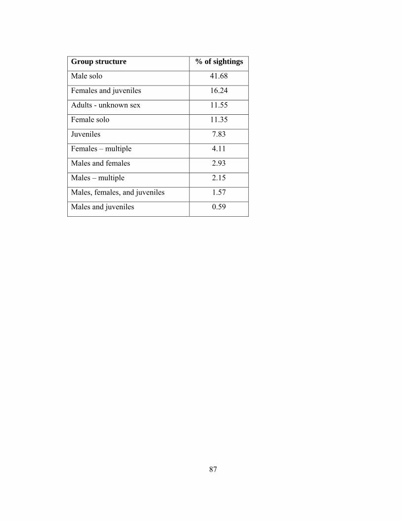
87

Group structure % of sightings

Male solo 41.68

Females and juveniles 16.24

Adults - unknown sex 11.55

Female solo 11.35

Juveniles 7.83

Females – multiple 4.11

Males and females 2.93

Males – multiple 2.15

Males, females, and juveniles 1.57

Males and juveniles 0.59

88

APPENDIX 2 Appendix 2. Daily activity time data collected from digital game cameras (infrared

Digital-Scout 3.2 megapixel; Penn’s Woods, Export, Pennsylvania, USA) placed

throughout both the control and treatment study areas to passively capture feral pigs at

Fort Benning, Georgia, August 2004 – May 2005. I baited 16 cameras with fermented

corn and moved them every 2 to 3 weeks in order to fully sample each study area several

times. I recorded activity time as the time the first sighting of each feral pig group

occurred during a 12 hour period. I recorded over 8200 photographs including 508

different activity time photographs for feral pigs groups.

89

Fig. 1

Daily activity time

0

10

20

30

40

50

60

0600

0800

1000

1200

1400

1600

1800

2000

2200

2400

0200

0400

Hour

# of

sig

htin

gs

Figure 1. Daily activity time of feral pigs at Fort Benning, Georgia, mid-August 2004 – May 2005.

90

Fig. 2

Daily activity time by season

02468

10121416

0600

0800

1000

1200

1400

1600

1800

2000

2200

2400

0200

0400

Hour

Prop

ortio

nal #

of s

ight

ings

FallWinterSpring

Figure 2. Activity time of feral pigs at Fort Benning, Georgia, 2004-2005 by season: fall = mid August – mid November, winter = mid November – mid February, spring = mid- February – May. To compare the number of sightings in each season, I computed a proportional number of sightings for each hour by dividing the number of sightings during that hour by the total number of sightings during that season.