demographics_and_mobility_report

Demographics and Mobility

Hajji Khalil, Master Student, Kafsi Mohamed, Student Member, Grossglauser Matthias, Member, Thiran Patrick, Senior Member

School of Computer and Communication Sciences, EPFL, CH-1015 Lausanne, Switzerland

ABSTRACT During the last years, the use of Internet has been moving from a static use to a mobile use. People are connected with their smartphone and tablets during all the day and they use Internet in all the places. They post Facebook messages in their work, they use Tweeter in their home, write comments on Trip Advisor in the restaurant they are eating in, upload Instagram photos of the building they are visiting. People are leaving a lot of traces about the places they use to visit and the activities they tend to do. As we are entering on the sphere of Big Data and Data Analysis, a lot of companies are investing a lot of resources and capacities to take profit from those public or private traces to better understand their users’ habits and behaviour. A lot of papers already tried to analyse the humans mobility and to predict their movement. Quan Yuan, Gao Cong, Zongyang Ma, Aixin Sun, Nadia Magnenat-Thalmann tried to predict in their paper “Who, Where, When and What: Discover Spatio-Temporal Topics for Twitter Users” the next location from where a person will do a tweet. Eunjoon Cho, Seth A.Myers and Jure Leskovec analyzed the mobility of humans in the location-based social networks in their paper “Friendship and Mobility: User Movement In Location-Based Social Networks”. In this paper we are taking benefits from the existence of such data and such work to try to answer to a more fundamental question: Is our mobility dictated by our social situation? Does the places that a person visits reveals some characteristics about him? Can we guess the age of a person looking only to the places he already visited? Can we guess his ethnicity? Answering to such questions could have a big impact in the human sciences domain: Human mobility is very complex and concluding that it is dictated by our social characteristics has important implications. Moreover, it could have an impact in the industrial world: Understanding their market segment and learning the preferences of their costumers is a competitive war that are leading a lot of companies. Keywords: Human mobility, Data analysis, Machine Learning, Generative Models 1. INTRODUCTION As independent humans, we tend to think that we have a big degree of freedom in our mobility. We believe that our movements are not predictable and that our choices of the places we decide to go in are not conditioned by our social characteristics. We will see in this paper that our mobility is more predictable than what we tend to think and that the places we visit exhibit a lot of characteristics about our person. In this work, we try to tackle the human mobility as a general problem and we are not focusing on a specific dataset. We made our best to propose models that can be used for any type of data containing mobility traces and that are able to answer to a various type of questions. This decision was motivated by two facts: First, the mobility traces could be different sources such as Tweeter data, Intagram data or some private mobile phone company data. The frequency of traces is in this case different, sometimes they represent a large sample of the mobility of a user and sometimes they reflect only a very small sample of it. Second, depending on the application, one may want to guess the ethnicity of the users or their gender or their age… Thus, the question that one is trying to answer may be different. Now that we explained the questions we are trying to answer and the goals that guided our work, it’s time to state the problem in a formal manner.

2 DEMOGRAPHICS AND MOBILITY

Let 𝑋! be the id of a place visited. 𝑋! could be for example the latitude-longitude coordinates of a place. 𝑋! will be called a check-in. Let 𝑋 = {𝑋!…𝑋!} be the set of the 𝑁 possible places where a person can do a check-in. 𝑋! is one of the values of 𝑋. The vector 𝑋 = [𝑋!… 𝑋!] represents a set of the places ordered by visit date 𝑋!… 𝑋!; 𝑋! is visited first, then 𝑋!, and 𝑋! is visited last. Let 𝐶 be a variable that represents the class of a person. 𝐶 can take some values {𝐶!…𝐶!} where 𝐶! represents a particular class. For example 𝐶 could represent the ethnicity of a person and takes values {"White", "Black", "Asian", "Hispanic", "Minority"}. Another example is when we want to classify tourists versus locals and then 𝐶 ∈ {"Local", "Tourist"} . In this work, our goal is to guess the class 𝐶 of a person 𝑢 based on the observation of the check-ins done by 𝑢, that are represented in a vector 𝑋. Thus our goal is to find a classification function 𝑓:𝑋 → 𝐶, which takes as input a vector of check-ins and outputs a class. In next sections, we will present two models of function 𝑓 that we developed, then we will describe the dataset we used to test our models. Finally, we will show the results we got with our two models and compare them to some baseline classifiers. 2. LATENT CLASS BEHAVIOUR (LCB) Our goal is to find a good model that expresses the Human mobility and then use this model to guess the class to which belongs a person. A good model comes at the start from good intuitions that are tuned later on into variables and equations. Thus, to understand our model, it is important to expose the intuitions that led us to it. 2.1- Intuitions

As individuals, how do we move? How do we choose the next places to go in? Obviously, we don’t choose randomly and we don’t have the same choices as others. Depending on the current state and on our personality, we will make a choice. In that sense, the movement of each individual is unique because each person will make different choices at some point. But is there something common in the movement of people? We believe that the response is yes and that even if the movements of each individual are unique, people exhibit some common behaviour in the places they visit. For example, some people like to go to the cinema on their free time, other to play sports; some people spend a lot of time at work, whereas other likes to stay at home. In that sense, we will not try to find patterns between the places that people visit but we will try to find patterns between the behaviours of people. This is our first intuition. Moreover, we believe that people that belong to the same class are likely to have similar behaviours, so that common patterns exist between the persons of the same class. In that sense, we will suppose that people of the same class have the same behaviours even if they don’t visit exactly the same places. This is where ‘Class Behaviour’ in the Latent Class Behaviour (LCB) comes from. This ends the explanation of our second intuition. 2.2- Model

The LCB is a probabilistic generative model. The behaviours are represented by a latent variable 𝑍 ∈ 𝑍!… 𝑍! where each 𝑍! , 𝑘 = 1…𝐾 represents a behaviour. In our context, behaviour represents a way to visit places (i.e. to do check-ins). So each behaviour 𝑍! is a distribution over the places of the set 𝑋 that we can express by 𝛽!! ,!! = Pr (𝑋 = 𝑋!|𝑍 = 𝑍!). The people belonging to the same class have the same behaviours so each class 𝐶 has a distribution over the different behaviours. This probability is expressed as 𝜋!,! = Pr (𝑍 = 𝑍!|𝐶 = 𝐶!). Let’s look at the generative model to have a better understanding. As suggests the graphical model (see figure 1), when a new person comes, it does the following: - First, it chooses a class 𝐶! ∈ {𝐶!…𝐶!} with probability 𝑃! = Pr (𝐶 = 𝐶!). -Second, knowing his class 𝐶!, he chooses a behaviour 𝑍! ∈ 𝑍!… 𝑍! with probability 𝜋!,! = Pr (𝑍 =𝑍!|𝐶 = 𝐶!).

-Finally, knowing his current behaviour 𝑍! , he visits a place 𝑋! ∈ {𝑋!…𝑋!} with probability 𝛽!! ,!! =Pr (𝑋 = 𝑋!|𝑍 = 𝑍!). To visit a new place, he selects again another behaviour with probability 𝜋!,! and then a place with probability 𝛽!! ,!! . Note here that he do not selects a class again. In fact, the class selection is done only once. This is because a person can only belong only to one class.

Figure 1: Graphical model of the LCB model. X is the observable, Z the hidden variable, C the

target variable

Let 𝑋 = [𝑋!… 𝑋!] be a check-in vector issued by a person, the likelihood of this observed vector 𝑋 in the LCB model is:

Pr 𝑋!,… ,𝑋! = 𝑃! 𝜋!,! ∙!

!!!

!

!!!

!

!!!

𝛽!!,!!

At this stage, we have a distribution but the 𝑃′𝑠, the 𝜋′𝑠 and the 𝛽′𝑠 are unknown. We suppose that our data is coming from this model and that the samples we are observing comes from this distribution. Starting from that, we will use the data we are observing to infer the 𝑃′𝑠, the 𝜋′𝑠 and the 𝛽′𝑠 that fit the best to our model. Once this is done, guessing the class 𝐶 of a person observing his check-ins 𝑋 = [𝑋!… 𝑋!] becomes straightforward:

𝑓 𝑋!… 𝑋! = 𝑎𝑟𝑔𝑚𝑎𝑥!! Pr 𝐶 = 𝐶! 𝑋!… 𝑋!

= 𝑎𝑟𝑔𝑚𝑎𝑥!!Pr (𝑋!… 𝑋!|𝐶 = 𝐶!) ∙ Pr (𝐶!)

Pr (𝑋!… 𝑋!)

= 𝑎𝑟𝑔𝑚𝑎𝑥!! Pr (𝑋!… 𝑋!|𝐶 = 𝐶!) ∙ Pr (𝐶!)

= 𝑎𝑟𝑔𝑚𝑎𝑥!! Pr (𝐶!) ∙ Pr (𝑋 = 𝑋!|𝐶 = 𝐶!)!

!!!

= 𝑎𝑟𝑔𝑚𝑎𝑥!! Pr 𝐶! ∙ Pr 𝑍 = 𝑍! 𝐶 = 𝐶! ∙ Pr 𝑋 = 𝑋! 𝑍 = 𝑍!

!

!!!

!

!!!

𝑓 𝑋!… 𝑋! = 𝑎𝑟𝑔𝑚𝑎𝑥!! Pr (𝐶!) ∙ 𝜋!,! ∙ 𝛽!!,!!

!

!!!

!

!!!

2.3- Learning parameters

As said in 2.2, to be able to make guesses, the learning of the parameters 𝑃, 𝜋 and 𝛽 is necessary. The last step before we close this section is to explain how the parameters are learnt.


2.3.1- Learning 𝑃

𝑃 is independent from the other quantities so we learn 𝑃 by simply maximizing the 𝑃 observed in the dataset we have. This is happens to be as the number of people belonging to each class divided by the total number persons. Thus,

𝑃! = Pr 𝐶 = 𝐶! = #𝑝𝑒𝑟𝑠𝑜𝑛𝑠_𝑜𝑓_𝑐𝑙𝑎𝑠𝑠_𝑚

#𝑡𝑜𝑡𝑎𝑙_𝑛𝑢𝑚𝑏𝑒𝑟_𝑜𝑓_𝑝𝑒𝑟𝑠𝑜𝑛𝑠

2.3.2- Learning Pi and Beta

Learning 𝜋 and 𝛽 is more complex. This is why the Expectation-Maximization (EM) algorithm is used to approach the best solutions of 𝜋 and 𝛽. Based on the fact that our model is a mixture of polynomials, we present below the Initialization-step, the E-Step and the M-Step. Initialization-step: We initialize randomly 𝜋 and 𝛽. E-step: We compute the responsibilities:

𝑟𝑠𝑝 𝑍! ,𝑋! ,𝐶! = Pr 𝑍 = 𝑍! 𝑋 = 𝑋! ,𝐶 = 𝐶! = 𝜋!,! ∙ 𝛽!!,!! This represents the probability that the check-in at 𝑋! generated by a person of class 𝐶! is coming from the topic 𝑍!. Then we normalize 𝑟𝑠𝑝 𝑍! ,𝑋! ,𝐶! such that:

𝑟𝑠𝑝 𝑍! ,𝑋! ,𝐶! = 1!!!…! . M-step: We update the 𝜋 and 𝛽:

𝜋!,! = 𝑟𝑠𝑝 𝑍! ,𝑋! ,𝐶! ∙ 𝑐𝑜𝑢𝑛𝑡(𝑋! ,𝐶!)!!∈{!!…!!}

𝛽!!,!! = 𝑟𝑠𝑝 𝑍! ,𝑋! ,𝐶! ∙ 𝑐𝑜𝑢𝑛𝑡(𝑋! ,𝐶!)!!∈{!!…!!}

where 𝑐𝑜𝑢𝑛𝑡 𝑋! ,𝐶! represents the number of times that the check-in 𝑋! appears in persons of class 𝐶!. Finally, we normalize 𝜋 and 𝛽 such that

𝜋!,! = 1!!!…!

𝛽!!,!! = 1!!∈{!!…!!}

The pseudo code below (Algorithm 1) presents how those steps are combined together to find the final value of 𝜋 and 𝛽. 2.3.2- The hyper parameter K

The variable 𝑍 represents the number of behaviours and can take values from 𝑍!… 𝑍! . The K represents the number of possible behaviours. This parameter is chosen by the user depending on the dataset and the classes he is trying to guess.

Algorithm 1: Expectation Maximization for LCB Input: check-in vectors 𝑋!,… ,𝑋! , the classes they belong to [𝐶!… ,𝐶!] and 𝐾 Output: 𝜋, 𝛽 𝜋, 𝛽 ← 𝑖𝑛𝑖𝑡𝑖𝑎𝑙𝑖𝑧𝑎𝑡𝑖𝑜𝑛 − 𝑠𝑡𝑒𝑝 while 𝑙𝑖𝑘𝑒𝑙𝑖ℎ𝑜𝑜𝑑 not converged

𝑟𝑠𝑝 ← 𝐸 − 𝑠𝑡𝑒𝑝 (𝜋, 𝛽) 𝜋, 𝛽 ← 𝑀 − 𝑠𝑡𝑒𝑝 (𝑟𝑠𝑝)

end while return 𝜋, 𝛽 3. LATENT PERSONALIZED BEHAVIOUR (LPB) In this section, we will present the Latent Personalized Behaviour (LPB) model. It’s an extension of LCB model where some hard characteristics of the LCB are relaxed in the LPB. 3.1- Intuitions

In LCB, all the behaviours are distributions over places. This means that people that belong to the same class have exactly the same probability to visit a given place. Is this true? Obviously it is not; two persons Alice and Bob that belongs to the same class should not have the same probability to visit Bob’s house. Behaviours are not only distribution over places, but they could also be distributions over places that have the same semantic to the persons that visits them. Alice and Bob do not have the same probability to visit Bob’s house because they belong to the same class. But because they belong to the same class, they could have the same probability to visit their respective home. The behaviour of Alice and Bob with respect to their respective home and respective work visit could be the same even if their home places and work places are not the same. Let’s illustrate this with one more example. Let’s suppose that our classes are {"Local", "Tourist"}. Based on people check-ins we would like to guess if they are locals or tourists. Despite the fact that it will be more probable for a local to check-in in the financial district than for a tourist, it is also true that a local will do check-ins in the places he use to visit whereas a tourist will do check-ins in more different places because he is discovering the city. In this case, the two classes have a different semantic behaviour that cannot be expressed by a distribution over places. In conclusion, people belonging to the same class could reveal some similar behaviour with respect to similar places in semantic but different in coordinates (example of Alice and Bob that visits their respective home in the same manner). In the other hand, people belonging to different classes could be differentiated thanks to behaviours with respect to the semantic. 3.2- Model

As in the LCB model, we suppose in the LPB model that each person has a couple of behaviours that are defined by the class he belongs to; each person has a distribution over behaviours that are completely defined by his class. Moreover, as in LCB, all the behaviours are distribution over places. Most of these distributions are common to all the people of the same class. However there is one behaviour that is unique for each person, i.e. a distribution over places that is unique for each person. It represents the distribution over the places already visited by a person. This means that each person will have some probability p to visit places he already visited, where p is common to all people of the same class. As we can note here, this behaviour models a semantic behaviour because p is common to all the class but the distribution over places depends only on the personal history of the person. This is why the model is called Latent-Personalized-Behaviour (LPB). Let’s see how this model solves the problems stated in 3.1. With the LPB, if Alice and Bob have the same behaviour with respect to their respective home, they will have approximately the same probability to visit their respective home. Indeed, they have the same probability to sample from places they already visited as they belong to the same class. Also, as they visit their respective home with the same frequency, they will have the same probability to sample their respective home from their already visited places.


Concerning the tourist and local classification, if our intuitions are true, the probability p will be much higher for the local than for the tourist. This exhibits the difference we talked about between the two classes. The LPB is a probabilistic generative model, with 𝐾 + 1behaviours represented in the variable 𝑍 ∈𝑍!… 𝑍!!! . The 𝑍! , 𝑘 = 1…𝐾 represent the behaviours as described in the LCB. The 𝑍!!! represents

the behaviour added in LPB model. The log-likelihood of LPB can be expressed as: Pr 𝑋!,… ,𝑋! = 𝑃! 𝜋!,! ∙!

!!!!!!!

!!!! 𝛽!!,!!

+ 𝜋!!!,! ∙ Pr (𝑋 = 𝑋!|𝑍 = 𝑍!!!,𝑋!,… ,𝑋!!!) It is important to note that in the LPB, the order of visits is important and the check-ins 𝑋 are no longer independent given the behaviour 𝑍 (see Figure 2). This is because when a person sample the behaviour 𝑍!!!, the probability of the next place he visits depends on the places he already visited.

Figure 2: Graphical model of the LPB model.

The parameters 𝑃, 𝜋 and 𝛽 need to be learned from the data before being able to guess. Once this is done, we can guess the class 𝐶 of a user observing his check-ins 𝑋 = [𝑋!… 𝑋!] in a similar manner than for LCB:

𝑓 𝑋!… 𝑋! = 𝑎𝑟𝑔𝑚𝑎𝑥!! Pr 𝐶 = 𝐶! 𝑋!… 𝑋!

= 𝑎𝑟𝑔𝑚𝑎𝑥!!Pr (𝑋!… 𝑋!|𝐶 = 𝐶!) ∙ Pr (𝐶!)

Pr (𝑋!… 𝑋!)

= 𝑎𝑟𝑔𝑚𝑎𝑥!! Pr (𝐶!) ∙ Pr (𝑋 = 𝑋!|𝐶 = 𝐶!)!

!!!

where

Pr (𝑋 = 𝑋!|𝐶 = 𝐶!)!

!!!

= ( 𝜋!,! ∙ 𝛽!!,!!

!

!!!

) + 𝜋!!!,! ∙ Pr (𝑋 = 𝑋!|𝑍 = 𝑍!!!,𝑋!…!!!)!

!!!

3.3- Learning Parameters

3.3.1- Learning 𝑃

Learning 𝑃 is done exactly in the same manner than in 2.3.1.

3.3.2- Learning 𝜋 and 𝛽

As in 2.3.2, we will use the EM algorithm to approximate 𝜋 and 𝛽. However, the equations of the E-Step and the M-Step become more complicated. First let’s note that 𝛽!! ,!! goes from 𝑘 = 1…𝐾. In fact, it does not include the distribution over the personal history of each user. Indeed, this probability is known from the observation of the places already visited by one person. Thus, it does not need to be learned.

Let 𝑋 𝑡 be the stochastic random variable that represents the place visited by a person 𝑢 at time 𝑡. Let 𝑍!(𝑡) represents the behaviour 𝑍! at time 𝑡. Finally we note that Pr (𝑋(𝑡) = 𝑋!|𝑍 = 𝑍!!!,𝑋 0 ,… ,𝑋(𝑡 − 1)) represents the personal history distribution of a user u. We omit the dependencies 𝑋 0 …𝑋(𝑡 − 1) in the notation for clarity reasons and we will write this distribution as:

Pr (𝑋(𝑡) = 𝑋!|𝑍 = 𝑍!!!,𝑢) Initialization-step: We initialize randomly 𝜋 and 𝛽. E-step: We compute the responsibilities for each user at each time step:

𝑟𝑠𝑝 𝑍! 𝑡 ,𝑋 𝑡 ,𝐶!,𝑢 = Pr 𝑍 𝑡 = 𝑍! 𝑋 𝑡 = 𝑋! ,𝐶 = 𝐶!,𝑢 = 𝜋!,! ∙ 𝛽!!,!! , 𝑘 = 1…𝐾

𝑟𝑠𝑝 𝑍! 𝑡 ,𝑋 𝑡 ,𝐶!,𝑢 = Pr 𝑍 𝑡 = 𝑍! 𝑋 𝑡 = 𝑋! ,𝐶 = 𝐶!,𝑢 = 𝜋!,! ∙ Pr 𝑋 𝑡 = 𝑋! 𝑍 = 𝑍!!!,𝑢 , 𝑘 = 𝐾 + 1

This represents the probability that the check-in at 𝑋! generated at time 𝑡 by a person 𝑢 of class 𝐶! is coming from the topic 𝑍!. Note that in this configuration, we have a responsibility for each person 𝑢 at each timestamp 𝑡. Then we normalize 𝑟𝑠𝑝 𝑍!(𝑡),𝑋(𝑡),𝐶!,𝑢 such that:

𝑟𝑠𝑝 𝑍!(𝑡),𝑋(𝑡),𝐶!,𝑢 = 1!!!…!!! . M-step: We update the 𝜋 and 𝛽:

𝜋!,! = 𝑟𝑠𝑝 𝑍! 𝑡 ,𝑋! 𝑡 ,𝐶!,𝑢!!∈{!!…!!}! !" !"#$$ !!!

𝛽!!,!! = 𝑟𝑠𝑝 𝑍! 𝑡 ,𝑋! 𝑡 ,𝐶!,𝑢! !" !"#$$ !!!!∈{!!…!!}!

Finally, we normalize 𝜋 and 𝛽 such that

𝜋!,! = 1!!!…!

𝛽!!,!! = 1!!∈{!!…!!}

3.3.2- Updating the personal history vector

Let 𝑋 = [𝑋!… 𝑋!] be the check-ins of a user 𝑢 . This personal history distribution represents the probability that 𝑢 makes a check-in a place he already visited 𝑋!. This is simply expressed as: Pr (𝑋(𝑡) = 𝑋!|𝑍 = 𝑍!!!,𝑋 0 ,… ,𝑋(𝑡 − 1)) = #!"_!"#$%&'(_!"#"$#_!"_!!

#!"!#$_!"_!"#$%&'(_!"#"$#

The distribution Pr (𝑋(𝑡) = 𝑋!|𝑍 = 𝑍!!!,𝑋 0 …𝑋(𝑡 − 1)) is updated after each check-in done by 𝑢.

3.3.3- The EM algorithm

to close this section, we present in Algorithm 2 who the steps described above are combined to execute this version of the EM algorithm. Note here that the E-step and the personal history update are combined. Finally, the hyper parameter 𝐾 is also fixed by the user.


Algorithm 2: Expectation Maximization for LPB Input: check-in vectors 𝑋!,… ,𝑋! , the classes they belong to [𝐶!… ,𝐶!] and 𝐾 Output: 𝜋, 𝛽 𝜋, 𝛽 ← 𝑖𝑛𝑖𝑡𝑖𝑎𝑙𝑖𝑧𝑎𝑡𝑖𝑜𝑛 − 𝑠𝑡𝑒𝑝 while 𝑙𝑖𝑘𝑒𝑙𝑖ℎ𝑜𝑜𝑑 not converged

foreach person 𝑢 foreach timestamp 𝑡

𝑟𝑠𝑝(𝑢, 𝑡) ← 𝐸 − 𝑠𝑡𝑒𝑝(𝑢, 𝑡,𝜋,𝛽) 𝑢𝑝𝑑𝑎𝑡𝑒 𝑝𝑒𝑟𝑠𝑜𝑛𝑎𝑙 ℎ𝑖𝑠𝑡𝑜𝑟𝑦 𝑣𝑒𝑟𝑐𝑡𝑜𝑟 𝑜𝑓 𝑢

end foreach end foreach 𝜋, 𝛽 ← 𝑀 − 𝑠𝑡𝑒𝑝(𝑟𝑠𝑝)

end while return 𝜋, 𝛽 4. DATASET Now that we explained the models we developed, it’s time to talk about the dataset we used to test the performances of our models. We built a dataset of Tweets in New York containing users tweets from 2011. The dataset contains 59513 users and 1035779 geo-localised tweets. In our context, a tweet represents a check-in and we are only interested in the coordinates of the localisation of the tweets. Here, the question we are asking is Can we guess the ethnicity of users based on their check-ins? The classes C are thus {"White", "Minority", " 𝑇𝑜𝑢𝑟𝑖𝑠𝑡"}. Even if the class " 𝑇𝑜𝑢𝑟𝑖𝑠𝑡" doesn’t represent an ethnicity, an Asian tourist will not behave as an Asian New-Yorker but he will behaves as a Tourist. That’s why we decided to add the category "Tourist" in our classes. 4.1- Labelling the Data

For each person we first decide if this person is a Tourist or a Local. If a person has New York as hometown (the hometown is a public information in Tweeter) or if we observed him more than 1 month in New York, then we can consider that he is a Local. If a person has a hometown different from New York, that we observed him less than 1 month and if the majority of his tweets are outside New York (i.e. he is not a new Tweeter user that lives in New York), then we consider this person as a Tourist (see Figure 3).

Figure 3: Local versus Tourist decision Graph.

Now for each Local person we will decide if he is a “White” or a “Minority”. For that, we use the dataset of the official US website www.census.gov. This database maps the most frequent American names to a distribution over ethnicities. Thus for each person, we get the ethnicity distribution that corresponds to his name and assign to him to most probable one. If it is "White", then we assign to him the class "White". Otherwise, we assign to him “𝑀𝑖𝑛𝑜𝑟𝑖𝑡𝑦”. 4.2- Data characteristics

As shown in the array of the Figure 4, the final distributions are 0.54 of "White", 0.3 of “𝑇𝑜𝑢𝑟𝑖𝑠𝑡” and 0.16 of “𝑀𝑖𝑛𝑜𝑟𝑖𝑡𝑦”. We can note that the classes of people are unbalanced. There is 2 more “𝑊ℎ𝑖𝑡𝑒” people than “𝑇𝑜𝑢𝑟𝑖𝑠𝑡” people and there is 2 more “𝑇𝑜𝑢𝑟𝑖𝑠𝑡” people than “𝑀𝑖𝑛𝑜𝑟𝑖𝑡𝑦”. We need to make attention that our classifiers will not classify always the majority class.

Figure 4: Dataset statistics. Class size and distribution.

The second observation we can make is that the number of check-ins by person follows a power-law (see Figure 5). There is a small number of people with a lot of tweets and a majority that has few tweets. This makes our guessing more challenging because the majority of persons we are trying to guess have very few traces.

Figure 5: Number of check-ins by user. Power-law distribution

Because our data is very sparse, the check-ins are aggregated by neighbourhood (Figure 6). Thus, for each person the observable are the neighbourhoods he visited and the goal is to guess the class of the person based on those visits. We will end this section by noting that 0.8 of the data is used for training and 0.2 is used for testing.


(a) New York divided by neighbourhood (b) check-ins number by neighbourhood. The

darker the colour, the more check-ins contains the neighbourhood.

Figure 6: New York City map

5. RESULTS In this section, we will first compare the LCB and the LPB performances to two baseline methods: The Support Vector Machine (SVM) and the Naïve Bayes. Then, we will show some interesting characteristics that are exposed by LCB and LPB. Finally, we will end this section by comparing LCB and LPB. 5.1- LCB LPB against baselines

For each class 𝐶! ∈ {“𝑊ℎ𝑖𝑡𝑒”, “𝑀𝑖𝑛𝑜𝑟𝑖𝑡𝑦”, ”𝑇𝑜𝑢𝑟𝑖𝑠𝑡”}, we compute the Accuracy for the class 𝐶! as:

𝐴𝑐𝑐𝑢𝑟𝑎𝑐𝑦!! =#𝑔𝑜𝑜𝑑_𝑐𝑙𝑎𝑠𝑠𝑖𝑓𝑖𝑐𝑎𝑡𝑖𝑜𝑛_𝑜𝑓_𝑐𝑙𝑎𝑠𝑠_𝐶!

#𝑡𝑜𝑡𝑎𝑙_𝑝𝑒𝑟𝑠𝑜𝑛𝑠_𝑜𝑓_𝑐𝑙𝑎𝑠𝑠_𝐶!

We also compute the total accuracy as:

𝑇𝑜𝑡𝑎𝑙_𝐴𝑐𝑐𝑢𝑟𝑎𝑐𝑦 =#𝑔𝑜𝑜𝑑_𝑐𝑙𝑎𝑠𝑠𝑖𝑓𝑖𝑐𝑎𝑡𝑖𝑜𝑛

#𝑡𝑜𝑡𝑎𝑙_𝑝𝑒𝑟𝑠𝑜𝑛𝑠

Finally, we compute the average accuracy as the mean of the accuracies of the all the classes:

𝐴𝑣𝑒𝑟𝑎𝑔𝑒_𝐴𝑐𝑐𝑢𝑟𝑎𝑐𝑦 =1𝑀∙ 𝐴𝑐𝑐𝑢𝑟𝑎𝑐𝑦!!

!

!!!

𝐴𝑣𝑒𝑟𝑎𝑔𝑒_𝐴𝑐𝑐𝑢𝑟𝑎𝑐𝑦 has the benefit that it gives the same weight to each class. In that case, the less represented classes will count with the same importance as the most represented ones. For that reason, we will rely on the 𝐴𝑣𝑒𝑟𝑎𝑔𝑒_𝐴𝑐𝑐𝑢𝑟𝑎𝑐𝑦 to test the performance of our classifiers. As said in 4.2, we divided our dataset into two sets: 80% that is used for training our classifiers and 20% is used for testing the performances of our classifiers. We run 4 different classifiers; the SVM, the Naive Bayes, the LCB and the LPB and the results obtained by those classifiers into the test set are presented in table below (see Figure 7). The Accuracies for each class are presented, so as to the 𝑇𝑜𝑡𝑎𝑙_𝐴𝑐𝑐𝑢𝑟𝑎𝑐𝑦 , the 𝐴𝑣𝑒𝑟𝑎𝑔𝑒_𝐴𝑐𝑐𝑢𝑟𝑎𝑐𝑦 and finally the log _𝑙𝑖𝑘𝑒𝑙𝑖ℎ𝑜𝑜𝑑.

We can see that the LPB and the LCB both outperform the SVM classifier. In fact they do 8% better than the SVM in the 𝐴𝑣𝑒𝑟𝑎𝑔𝑒_𝐴𝑐𝑐𝑢𝑟𝑎𝑐𝑦 and respectively 6% and 9% better in the 𝑇𝑜𝑡𝑎𝑙_𝐴𝑐𝑐𝑢𝑟𝑎𝑐𝑦. We can see that they also do better than the Naive Bayes. In fact, even if the LPB has the same performance than the Naive Bayes for the 𝑇𝑜𝑡𝑎𝑙_𝐴𝑐𝑐𝑢𝑟𝑎𝑐𝑦, both LPB and LCB do 2% better in the 𝐴𝑣𝑒𝑟𝑎𝑔𝑒_𝐴𝑐𝑐𝑢𝑟𝑎𝑐𝑦. This means that they guess better the ethnicities even if there is some minority represented. Finally, the log _𝑙𝑖𝑘𝑒𝑙𝑖ℎ𝑜𝑜𝑑 shows that the LCB and the LPB makes the data much more predictable than the Naive Bayes.

Figure 7: Classifiers performances table

5.2- Zoom in LCB LPB

In this section we will have a deeper look into the two models we presented in this work and we will see which model is better to use depending on the situation. We can see from the Figure 7 that the LCB performs better in guessing “𝑊ℎ𝑖𝑡𝑒” and “𝑀𝑖𝑛𝑜𝑟𝑖𝑡𝑦”. As the White class represents 54% of the data, this explains why LCB has a better score in 𝑇𝑜𝑡𝑎𝑙_𝐴𝑐𝑐𝑢𝑟𝑎𝑐𝑦. However, LPB performs much better in guessing the "𝑇𝑜𝑢𝑟𝑖𝑠𝑡" class; indeed, approximately 3 tourists over 4 are guessed correctly. The 𝐴𝑣𝑒𝑟𝑎𝑔𝑒_𝐴𝑐𝑐𝑢𝑟𝑎𝑐𝑦 shows us that in mean, both LCB and PCB have the same performance as they both perform to 0.42%. So depending on the kind of application, one may prefer to choose LCB or LPB. Another interesting way to look at the results is to look at the graph shown in Figure 8. This graph shows the probability of error obtained with people that have different numbers of check-ins. We can see that probability of error of LCB and LPB decrease exponentially when the number of check-ins increases. It reaches 0.3 after some samples. The two curves follow a power law. We can also see that after 5 check-ins, the probability of error of LCB and LPB becomes stable around the value of 0.3. This means that we only need 5 samples to be able to guess with a good confidence the category of a person and the check-ins above this number do not add information to the predictors. Furthermore, we can see that the LCB performs better when the person has few check-ins but the LPB does better when the number of check-ins is ≥ 3. Thus, the LCB could be a good choice when the dataset is very sparse whereas the LPB is a better choice when we have a more complete data.

Figure 8: The probability of error in function of the number of check-ins


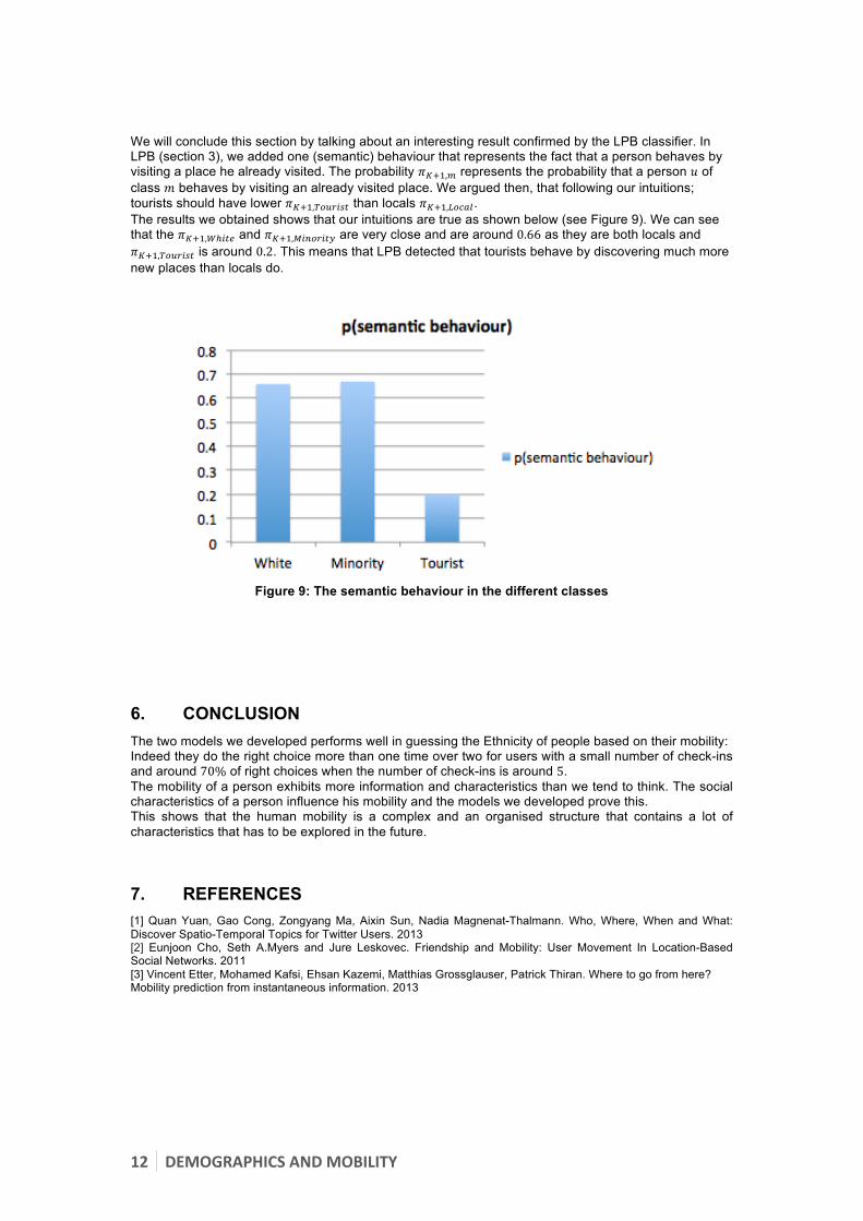
We will conclude this section by talking about an interesting result confirmed by the LPB classifier. In LPB (section 3), we added one (semantic) behaviour that represents the fact that a person behaves by visiting a place he already visited. The probability 𝜋!!!,! represents the probability that a person 𝑢 of class 𝑚 behaves by visiting an already visited place. We argued then, that following our intuitions; tourists should have lower 𝜋!!!,!"#$%&' than locals 𝜋!!!,!"#$%. The results we obtained shows that our intuitions are true as shown below (see Figure 9). We can see that the 𝜋!!!,!!!"# and 𝜋!!!,!"#$%"&' are very close and are around 0.66 as they are both locals and 𝜋!!!,!"#$%&' is around 0.2. This means that LPB detected that tourists behave by discovering much more new places than locals do.

Figure 9: The semantic behaviour in the different classes

6. CONCLUSION The two models we developed performs well in guessing the Ethnicity of people based on their mobility: Indeed they do the right choice more than one time over two for users with a small number of check-ins and around 70% of right choices when the number of check-ins is around 5. The mobility of a person exhibits more information and characteristics than we tend to think. The social characteristics of a person influence his mobility and the models we developed prove this. This shows that the human mobility is a complex and an organised structure that contains a lot of characteristics that has to be explored in the future. 7. REFERENCES [1] Quan Yuan, Gao Cong, Zongyang Ma, Aixin Sun, Nadia Magnenat-Thalmann. Who, Where, When and What: Discover Spatio-Temporal Topics for Twitter Users. 2013 [2] Eunjoon Cho, Seth A.Myers and Jure Leskovec. Friendship and Mobility: User Movement In Location-Based Social Networks. 2011 [3] Vincent Etter, Mohamed Kafsi, Ehsan Kazemi, Matthias Grossglauser, Patrick Thiran. Where to go from here? Mobility prediction from instantaneous information. 2013

Documents

demographics_and_mobility_report