Demographics and the Evolution of Global Imbalances

Michael Sposi Federal Reserve Bank of Dallas

System Working Paper 18-09 March 2018

The views expressed herein are those of the authors and not necessarily those of the Federal Reserve Bank of Minneapolis or the Federal Reserve System. This paper was originally published as Globalization and Monetary Policy Institute Working Paper No. 332 by the Federal Reserve Bank of Dallas. This paper may be revised. The most current version is available at https://doi.org/10.24149/gwp332. __________________________________________________________________________________________

Opportunity and Inclusive Growth Institute Federal Reserve Bank of Minneapolis • 90 Hennepin Avenue • Minneapolis, MN 55480-0291

https://www.minneapolisfed.org/institute

Federal Reserve Bank of Dallas Globalization and Monetary Policy Institute

Working Paper No. 332 https://doi.org/10.24149/gwp332

Demographics and the Evolution of Global Imbalances*

Michael Sposi Federal Reserve Bank of Dallas

December 2017

Abstract The working age share of the population has evolved, and will continue to evolve, asymmetrically across countries. I develop a dynamic, multicountry, Ricardian trade model with endogenous labor supply to quantify how these asymmetries systematically affect the pattern of trade imbalances across 28 countries from 1970-2014. Changes in both domestic and foreign working age shares impact a country's net exports directly through the demand for net saving and indirectly through relative labor supply and population growth. Counterfactually removing demographic-induced changes to saving unveils a strong negative contemporaneous relationship between net exports and productivity growth. Demographics, thus, alleviate the allocation puzzle, and do so to a greater degree than investment distortions. Neither labor market distortions nor trade distortions systematically reconcile the puzzle.

JEL codes: F11, F21, J11

* Michael Sposi, Federal Reserve Bank of Dallas, Research Department, 2200 N. Pearl Street, Dallas, TX75201. 214-922-5881. michael.sposi@dal.frb.org. I am grateful to Mick Devereux, Jonathan Eaton, KarenLewis, Kanda Naknoi, Kim Ruhl, Mark Wynne, and Kei-Mu Yi for helpful comments. This paper alsobenefited from audiences at the Bank of Canada, Dallas Fed, Penn State, University of Toronto, andUniversity of Connecticut. Kelvin Virdi provided excellent research assistance. The views in this paper arethose of the author and do not necessarily reflect the views of the Federal Reserve Bank of Dallas or theFederal Reserve System.

1 Introduction

As of 2014, the absolute value of net exports summed across 182 countries amounted to 5.2

percent of world GDP (version 9.0 of the Penn World Table). These imbalances entailed

net inflows of resources for some countries and net outflows for others. For instance, for

the United States imports exceeded exports by 4.2 percent of GDP, while for China imports

fell short of exports by 3.7 percent of GDP. In most countries both the direction and the

magnitude of trade imbalances are highly persistent over time, yet, little is known about what

factors systematically determine imbalances across the world in the long run. Since trade

imbalances reflect both intertemporal and intratemporal resource allocations, implications

for policies that target trade and current accounts hinge on understanding the drivers.

Existing research has focussed on the effects of cross-country differences in factors such

as productivity growth, trade barriers, institutions, and various distortions; few papers have

studied the role of demographics. Demographics offer a promising candidate since they have

direct implications for aggregate saving and are persistent over time. General equilibrium

analyses linking demographics to trade imbalances have used two-country, or at most three-

country, models (e.g., Ferrero, 2010; Krueger and Ludwig, 2007). Multicountry analyses have

been empirical (e.g., Alfaro, Kalemli-Ozcan, and Volosovych, 2008; Higgins, 1998).

This paper builds a dynamic, multicountry, Ricardian trade model to study how demo-

graphics systematically affect the pattern of trade imbalances across 28 countries since 1970.

Countries are integrated via bilateral trade linkages and can borrow and lend with each other.

Dynamics are driven by saving in one-period international bonds and investment in physical

capital. Labor supply is endogenous. Both contemporaneous and projected demographics

affect trade imbalances directly through saving demand and indirectly through labor supply

and population growth. To my knowledge, this is the first model to combine all of these

features in a multicountry environment and deliver exact transitional dynamics.

I find that cross-country differences in changes to the working age share helps system-

atically explain both the direction and magnitude of trade imbalances. The findings shed

new light on the allocation puzzle. The puzzle begins with a clear prediction from economic

theory: Slow-growing countries should run trade surpluses and, fast-growing countries, trade

deficits.1 However, a great deal of empirical evidence stands in contrast to this prediction

(see Gourinchas and Jeanne, 2013; Prasad, Rajan, and Subramanian, 2007). In my sample

1The allocation puzzle is often discussed in terms of the current account. All of the facts and findingsthat I describe in terms of the trade balance are also true in terms of the current account balance.

2

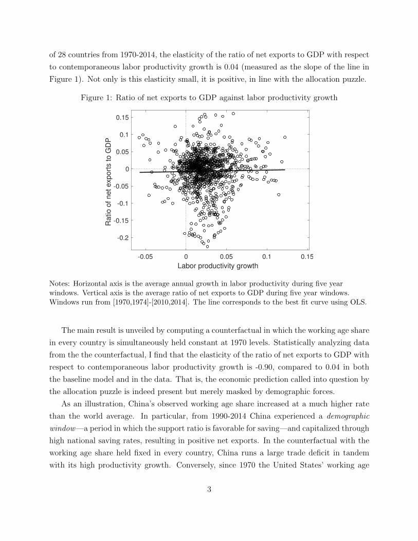
of 28 countries from 1970-2014, the elasticity of the ratio of net exports to GDP with respect

to contemporaneous labor productivity growth is 0.04 (measured as the slope of the line in

Figure 1). Not only is this elasticity small, it is positive, in line with the allocation puzzle.

Figure 1: Ratio of net exports to GDP against labor productivity growth

-0.05 0 0.05 0.1 0.15

Labor productivity growth

-0.2

-0.15

-0.1

-0.05

0

0.05

0.1

0.15

Ra

tio

of

ne

t e

xp

ort

s t

o G

DP

Notes: Horizontal axis is the average annual growth in labor productivity during five yearwindows. Vertical axis is the average ratio of net exports to GDP during five year windows.Windows run from [1970,1974]-[2010,2014]. The line corresponds to the best fit curve using OLS.

The main result is unveiled by computing a counterfactual in which the working age share

in every country is simultaneously held constant at 1970 levels. Statistically analyzing data

from the the counterfactual, I find that the elasticity of the ratio of net exports to GDP with

respect to contemporaneous labor productivity growth is -0.90, compared to 0.04 in both

the baseline model and in the data. That is, the economic prediction called into question by

the allocation puzzle is indeed present but merely masked by demographic forces.

As an illustration, China’s observed working age share increased at a much higher rate

than the world average. In particular, from 1990-2014 China experienced a demographic

window—a period in which the support ratio is favorable for saving—and capitalized through

high national saving rates, resulting in positive net exports. In the counterfactual with the

working age share held fixed in every country, China runs a large trade deficit in tandem

with its high productivity growth. Conversely, since 1970 the United States’ working age

3

share increased at a slower rate compared to the world average. In the counterfactual the

U.S. trade balance fluctuates around zero.

The model is calibrated to 27 countries and a rest-of-world aggregate from 1970-2060.

Data from 1970-2014 are observed, while data for 2015-2060 are based on long-term projec-

tions. Incorporating projections provides external discipline to households’ expectations in

formulating saving decisions during the period of interest: 1970-2014. It also significantly

reduces the impact that terminal conditions impose on the saving behavior during that pe-

riod. I employ a wedge-accounting procedure that assigns parameter values to rationalize

both the observed and the projected data as a solution to a perfect-foresight equilibrium.2

In the model each country is populated by a representative household, so there is no

explicit notion of heterogeneity in age either within or across countries. Instead, information

about the age distribution is embedded in three parameters: (i) saving wedges (changes

in the discount factor), (ii) labor wedges (marginal utility of leisure), and (iii) population

growth rates. I provide microfoundations to illustrate the mapping between the parameters

and changes in the age distribution arising from an overlapping-generations framework. The

microfoundations guide an empirical decomposition of these parameters into a demographic

component and a non-demographic (distortionary) component.3 The decomposition serves

as a disciplining device to study counterfactuals in which alterations to the working age share

are manifested in alterations to the three parameters.

Each parameter provides a distinct channel through which demographics affect trade

imbalances. First, a higher working age share implies a higher saving wedge, i.e., a greater

demand for future consumption relative to current consumption. Resultantly there will be

higher contemporaneous demand for saving and higher net exports.

Second, a higher working age share implies a lower labor wedge, which in turn implies

higher labor supply and productive capacity. As a result, a country will borrow less to fund

its liabilities and will have contemporaneously higher demand for saving and net exports.

Third, a higher working age share implies lower population growth. When population

growth is relatively low, agents will save less to ensure that consumption is smoothed out

2Wedge accounting has its roots in business cycle accounting (see Chari, Kehoe, and McGrattan, 2007).Eaton, Kortum, Neiman, and Romalis (2016) modified the procedure to encompass a dynamic trade model.One key difference from them is that my solution procedure solves for the decentralized competitive alloca-tions, whereas their’s assumes fixed Pareto weights, which forces each country’s share in global consumptionto be counterfactually invariant with respect to the baseline. In my model these weights endogenously changein each counterfactual.

3Since the wedges fully account for each country’s saving behavior, the distortionary component capturesnon-demographic aspects pointed to by the literature, including financial market distortions.

4

over time on a per capita basis. Novel to the open economy model is that population size

affects the terms of trade and real interest rate differentials across countries, a channel that

is under appreciated in the literature. A relatively lower population level implies a higher

real exchange rate, all else equal. Therefore, lower population growth implies relatively

improving terms of trade over time and, in turn, a relatively higher real interest rate, which

supports the greater demand for saving and higher net exports.

Each country’s net exports is influenced by both domestic and foreign demographics.

I find that net exports respond more to domestic demographics, relative to foreign demo-

graphics, in countries in which the working age share evolved more differently from the world

average. For example, China’s trade balance was driven more by changes in its own demo-

graphics and China’s working age share increased significantly faster than that of the world.

Conversly, the U.S. trade balance was influenced more by changes in foreign demographics

and the U.S. working age share increased slightly slower than, but at a fairly similar rate as,

that of the world.

Because trade imbalances encompass both intertemporal and intratemporal margins, it

is useful to consider the ratio of net exports to GDP as the product of (i) the ratio of net

exports to trade (imports plus exports) and (ii) the ratio of trade to GDP. Loosely speaking,

the ratio of net exports to trade as reflects intertemporal margins, i.e., saving, that govern

direction of net trade and capital flows. The ratio of trade to GDP reflects intratemporal

margins, i.e., trade distortions, that govern the volume of gross trade flows and openness.

Two distinct literatures have emerged studying each margin.

My paper connects, and builds on, these literatures by systematically addressing both the

intertemporal margin (direction of net trade) as well as the intratemporal margin (volume

of trade) by matching the observed bilateral trade flows and, hence, bilateral and aggregate

trade balances across many countries in a general equilibrium framework.

The literature on imbalances and capital flows can be traced to Lucas (1990), who ques-

tions why capital does not flow from rich to poor countries. That is, in the long run, the

marginal product of capital (MPK) should equalize, requiring similar capital-labor ratios.

While this is still an open question, Caselli and Feyrer (2007) show that after adjusting for

differences in the relative price of capital across countries, real MPKs are not very different.

Because of this, my model is disciplined to match the observed relative prices.

Recently, attention has focussed on understanding why capital does not flow into fast

growing countries, i.e., the allocation puzzle. A number of explanations have been put

forward. Carroll, Overland, and Weil (2000) posit that habits can account for the fact that

5

a boom income is not immediately met with a boom in consumption. Instead, fast growing

countries will tend to save in the short run. However, this answer does not address why

saving winds up in net exports as opposed to investment. Along these lines Aguiar and

Amador (2011) argue that fast growing economies with high debt will not invest capital due

to the risk of expropriation. Instead, governments in these economies have an incentive to

pay down debt. Buera and Shin (2017) argue that financial frictions restrict the extent that

investment can respond to fast GDP growth, implying that a fast growing country will tend

to run a current account surplus in the short run. Ohanian, Restrepo-Echavarria, and Wright

(2017) point to labor market frictions as being an important ingredient. They argue that,

after World War II, labor wedges in Latin America impeded equilibrium supply of labor,

thereby reducing the marginal product of capital and repelling foreign investment.

Each of these explanations sheds light on idiosyncratic episodes of abnormally high

growth, but none systematically consider a large number of countries over a long time

period. Looking across 28 countries from 1970-2014, I find that investment distortions

partially alleviate the allocation puzzle, but are less important than demographics. La-

bor market distortions do not reconcile the puzzle in my sample. The underlying economics

are straightforward: trade imbalances appear in the current account, which embodies net

saving. Gourinchas and Jeanne (2013) argue that the allocation puzzle is one about saving—

not investment—and more specifically about public saving. Public saving is driven in large

part by pensions, where current and projected assets and liabilities depend on current and

projected demographics. Asymmetries in demographic changes provide an incentive for in-

tertemporal trade to balance assets and liabilities.

A separate, albeit related, literature explicitly investigates the role of trade openness in

explaining imbalances. Using a multicountry model, Reyes-Heroles (2016) argues that the

increased ratio of global trade to global GDP accounts for the rise in the ratio of global

imbalances to global GDP. He argues declining trade costs over time generate larger trade

volumes, thereby amplifying the net trade positions as a share of GDP. His analysis does

not focus on explaining heterogeneity in country-level imbalances.

Alessandria and Choi (2017) document that the ratio of U.S. net exports to GDP in-

creased in absolute value because trade increased as a share of GDP, while the ratio of

net exports to trade has been relatively stationary. They argue that U.S. import barriers

declined faster than U.S. export barriers, and that this asymmetry helps explain both the

magnitude and the direction of the U.S. trade imbalance. I find that asymmetries in bilateral

trade barriers help explain the temporary widening of the U.S. trade deficit since 2000, while

6

demographics capture the persistent widening since the 1980s. Changes in bilateral trade

barriers do not systematically reconcile the allocation puzzle across many countries.

China is well-cited example of a country with rapid growth and large trade surplus. Wei

and Zhang (2011) argue that male-biased gender ratios encourage men to save by purchasing

real estate to attract scarce female partners. Yang, Zhang, and Zhou (2012) argue that

successive cohorts of young Chinese workers face increasingly flat life-cycle earnings profiles,

thereby reducing household borrowing in the face of higher future aggregate productivity.

Imorohoglu and Zhao (2017a) argue that, due to China’s one-child policy, the elderly rely

more on personal savings to replace lacking family support during retirement. Imorohoglu

and Zhao (2017b) argue that financial constraints faced by firms is equally important as the

one-child policy in accounting for the rise in China’s saving rate. In Song, Storesletten, and

Zilibotti (2011), financial market imperfections imply that private firms in China finance

the adaptation of technology through internal savings. My findings do not rule out any of

these theories but, instead, offer a systematic assessment of the role of demographic-induced

saving behavior across many countries over a long time period.

My modeling approach differs slightly from those found in previous studies on demo-

graphics and trade imbalances. Krueger and Ludwig (2007) study demographics in an open

economy with overlapping generations. However, their model considers only three coun-

tries. Ferrero (2010) incorporates demographics into a two-country model with two types of

agents: workers and retirees. Workers transition into retirement with a time-varying proba-

bility making the problem mimic that of a representative agent. Their approach is similar to

that developed by Blanchard (1985), who shows that a representative-agent model can mimic

outcomes from an overlapping generations model where agents face a constant probability

of death in each period. My paper abstracts from the overlapping generations structure

and instead uses a representative household whose preferences change over time based on

changes in the age distribution. This enables me to avoid value functions, which are far too

intractable in a general equilibrium environment with a large number of countries.

Methodologically, this paper contributes to a recent strand of literature incorporating

dynamics into multicountry trade models (Alvarez, 2017; Caliendo, Dvorkin, and Parro, 2015;

Eaton, Kortum, Neiman, and Romalis, 2016; Ravikumar, Santacreu, and Sposi, 2017; Reyes-

Heroles, 2016; Sposi, 2012; Zylkin, 2016). I extend the algorithm developed in Ravikumar,

Santacreu, and Sposi (2017) to incorporate endogenous labor supply.4

4Adao, Arkolakis, and Esposito (2017) incorporate endoegnous labor supply into a static multicountrytrade model.

7

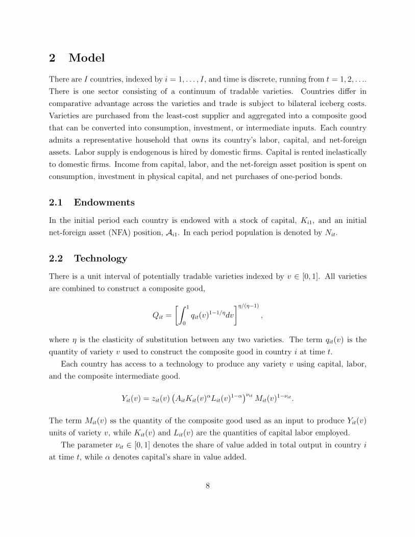
2 Model

There are I countries, indexed by i = 1, . . . , I, and time is discrete, running from t = 1, 2, . . ..

There is one sector consisting of a continuum of tradable varieties. Countries differ in

comparative advantage across the varieties and trade is subject to bilateral iceberg costs.

Varieties are purchased from the least-cost supplier and aggregated into a composite good

that can be converted into consumption, investment, or intermediate inputs. Each country

admits a representative household that owns its country’s labor, capital, and net-foreign

assets. Labor supply is endogenous is hired by domestic firms. Capital is rented inelastically

to domestic firms. Income from capital, labor, and the net-foreign asset position is spent on

consumption, investment in physical capital, and net purchases of one-period bonds.

2.1 Endowments

In the initial period each country is endowed with a stock of capital, Ki1, and an initial

net-foreign asset (NFA) position, Ai1. In each period population is denoted by Nit.

2.2 Technology

There is a unit interval of potentially tradable varieties indexed by v ∈ [0, 1]. All varieties

are combined to construct a composite good,

Qit =

[∫ 1

0

qit(v)1−1/ηdv

]η/(η−1)

,

where η is the elasticity of substitution between any two varieties. The term qit(v) is the

quantity of variety v used to construct the composite good in country i at time t.

Each country has access to a technology to produce any variety v using capital, labor,

and the composite intermediate good.

Yit(v) = zit(v)(AitKit(v)αLit(v)1−α)νitMit(v)1−νit .

The term Mit(v) ss the quantity of the composite good used as an input to produce Yit(v)

units of variety v, while Kit(v) and Lit(v) are the quantities of capital labor employed.

The parameter νit ∈ [0, 1] denotes the share of value added in total output in country i

at time t, while α denotes capital’s share in value added.

8

The term Ait denotes country i’s value-added productivity at time t while the term zit(v)

is country i’s idiosyncratic productivity draw for producing variety v at time t, which scales

gross output. Idiosyncratic productivity in each country is drawn independently from a

Frechet with cumulative distribution function F (z) = exp(−z−θ).

2.3 Trade

International trade is subject to iceberg trade barriers. At time t, country i must purchase

dijt ≥ 1 units of any intermediate variety from country j in order for one unit to arrive;

dijt − 1 units melt away in transit. As a normalization I assume that diit = 1 for all i and t.

2.4 Preferences

The representative household’s preferences are defined over consumption per capita, CitNit

, and

labor supply per capita (hours), LitNit

, over the lifetime.

∞∑t=1

βt−1ψitNit U(CitNit

,LitNit

).

Utility between adjacent periods is discounted by β ∈ (0, 1). The parameter ψit is a discount-

factor shock in country i at time t, meaning that ψit/ψit−1—“saving wedge” from now on—is

a shock to the marginal rate of substitution between consumption in adjacent time periods.

The period-utility function is given by

U(CitNit

,LitNit

)=

(Cit/Nit)1−1/σ

1− 1/σ+ ζit

(1− Lit/Nit)1−1/φ

1− 1/φ.

The term σ denotes the intertemporal elasticity of substitution for consumption with respect

to the real interest rate, while φ denotes the elasticity of labor supply with respect to the

real wage. Both parameters are constant across countries and over time. The term ζit is a

shock to the marginal utility of leisure—’‘labor wedge” from now on—in country i at time t.

Both the saving wedge and the labor wedge can equivalently be modeled as distortions to

net-foreign income and labor income, respectively. I include these wedges in the preferences

to emphasize the idea that they incorporate demographic forces that influence the relative

demand for saving and the optimal labor supply, even in the absence of distortions. Later

on I provide micro foundations to justify this assumption. At which point, I decompose the

wedges into distinct demographic and distortionary components.

9

Demographics The model does not explicitly include heterogeneity in age. Instead,

variation in demographics across countries and over time is manifested in (i) the saving

wedge, (ii) the labor wedge, and (iii) population growth. A main goal of the quantitative

exercise is to isolate the variation in these wedges that comes from variation in demographics.

Net-foreign asset accumulation The representative household enters period t with

NFA position Ait. If Ait < 0 then the household has a net debt position. It is augmented

by net purchases of one-period bonds (the current account balance), Bit. With Ai1 given:

Ait+1 = Ait + Bit.

Capital accumulation The household enters period t with Kit units of capital. A

fraction δ depreciates during the period. Investment, Xit, adds to the stock of capital subject

to an adjustment cost. Thus, with Ki1 > 0 given, the capital accumulation technology is

Kit+1 = (1− δ)Kit + δ1−λXλitK

1−λit .

The depreciation rate, δ, and the adjustment cost elasticity, λ, are constant both across

countries and over time. The term δ1−λ ensures that there are no adjustment costs to

replace depreciated capital; for instance, in a steady state X? = δK?. The adjustment cost

implies that the return to capital investment is not invariant to the quantity of investment.

In turn, the household always chooses a unique portfolio of capital and bonds at any prices.

Budget constraint Capital and labor are compensated at the rates rit and wit, re-

spectively. Capital income is subject to a distortionary tax, τ kit, while current investment

expenditures are tax deductible. Tax revenue is returned in lump sum to the household, Tit.

The world interest rate on outstanding debt at time t is denoted by qt. If the household

has a positive NFA position at time t, then net foreign income, qtAit, is positive. Otherwise

net foreign income is negative as resources must be spent to service existing liabilities.

The composite good has price Pit and can be transformed into χcit units of consumption

or into χxit units of investment. These transformation costs pin down relative prices and are

needed to reconcile the Lucas (1990) paradox (see Caselli and Feyrer, 2007). The budget

constraint in each period is given by

PitχcitCit + Bit =

(ritKit −

PitχxitXit

)(1− τ kit) + witLi + qtAit + Tit.

10

2.5 Equilibrium

A competitive equilibrium satisfies the following conditions: (i) taking prices as given, the

representative household in each country maximizes its lifetime utility subject to its budget

constraint and technologies for accumulating physical capital and assets, (ii) taking prices as

given, firms maximize profits subject to the available technologies, (iii) intermediate varieties

are purchased from their lowest-cost provider, and (iv) markets clear. At each point in time

world GDP is the numeraire:∑I

i=1 ritKit + witLi = 1. That is, all prices are expressed in

units of current world GDP. Appendix D describes the equilibrium conditions in more detail.

3 Calibration

The model is applied to 28 countries (27 individual countries plus a rest-of-world aggregate)

from 1970-2060. Data from 1970-2014 are realized, while data from 2015-2060 are based on

projections. Incorporating projections serves two purposes. First, it imposes the terminal

conditions as of 2060, which has minimal effects on the saving behavior from 1970-2014, which

is the period of interest. Second, it provides external discipline to the agents expectations in

formulating saving decisions prior to 2014. Appendix C provides a description of the data

along with a list of the countries and their 3-digit ISO codes.

The calibration involves two parts. The first part assigns values to parameters that

are common across countries and constant over time: (θ, η, δ, λ, α, β, σ, φ). These are taken

off the shelf from the literature. The second part assigns values to country-specific and

time-varying parameters: (Ki1,Ai1) and {Nit, χcit, χ

xit, νit, ψit, ζit, τ

kit, dijt, Ait}Tt=1 for all (i, j, t).

These parameters are inferred to rationalize both the observed and projected data as a

solution to a perfect foresight equilibrium. The data targets, roughly in order of how they

map into the model parameters, are (i) initial stock of capital, (ii) initial NFA position,

(iii) population, (iv) price level of consumption using PPP exchange rates, (v) price level of

investment using PPP exchange rates, (vi) ratio of value added to gross output, (vii) real

consumption, (viii) ratio of employment to population, (ix) real investment, (x) bilateral

trade flows, and (xi) price level of tradables using PPP exchange rates.

The saving wedge, the labor wedge, and population growth each play a role in tying de-

mographic forces to the model. The remaining parameters are used to match other important

aspects of data to ensure internal consistency with national accounts.

11

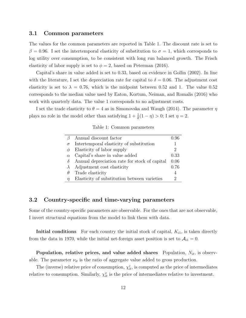
3.1 Common parameters

The values for the common parameters are reported in Table 1. The discount rate is set to

β = 0.96. I set the intertemporal elasticity of substitution to σ = 1, which corresponds to

log utility over consumption, to be consistent with long run balanced growth. The Frisch

elasticity of labor supply is set to φ = 2, based on Peterman (2016).

Capital’s share in value added is set to 0.33, based on evidence in Gollin (2002). In line

with the literature, I set the depreciation rate for capital to δ = 0.06. The adjustment cost

elasticity is set to λ = 0.76, which is the midpoint between 0.52 and 1. The value 0.52

corresponds to the median value used by Eaton, Kortum, Neiman, and Romalis (2016) who

work with quarterly data. The value 1 corresponds to no adjustment costs.

I set the trade elasticity to θ = 4 as in Simonovska and Waugh (2014). The parameter η

plays no role in the model other than satisfying 1 + 1θ(1− η) > 0; I set η = 2.

Table 1: Common parameters

β Annual discount factor 0.96σ Intertemporal elasticity of substitution 1φ Elasticity of labor supply 2α Capital’s share in value added 0.33δ Annual depreciation rate for stock of capital 0.06λ Adjustment cost elasticity 0.76θ Trade elasticity 4η Elasticity of substitution between varieties 2

3.2 Country-specific and time-varying parameters

Some of the country-specific parameters are observable. For the ones that are not observable,

I invert structural equations from the model to link them with data.

Initial conditions For each country the initial stock of capital, Ki1, is taken directly

from the data in 1970, while the initial net-foreign asset position is set to Ai1 = 0.

Population, relative prices, and value added shares Population, Nit, is observ-

able. The parameter νit is the ratio of aggregate value added to gross production.

The (inverse) relative price of consumption, χcit, is computed as the price of intermediates

relative to consumption. Similarly, χxit is the price of intermediates relative to investment.

12

Saving wedges The saving wedges are only identified up to I − 1 countries at each

point in time. As such, I normalize ψUt = 1 for all t (subscript U denotes the United States).

Appealing to the Euler equation for bonds in the United States, the implied world interest

rate is recovered using data on the paths for U.S. population, prices, and consumption:

Cit+1/Nit+1

Cit/Nit

= βσ(ψit+1

ψit

)σ 1 + qt+1

Pit+1/χcit+1

Pit/χcit

σ

.

Given the world interest rate, qt, saving wedges in every other country are recovered from

the respective Euler equations for bonds. I normalize ψi1 = 1 in every country.

Labor wedges The labor wedges are pinned down by exploiting the optimal labor-

supply condition and utilizing data on wages, prices, employment, and consumption:

1− LitNit

= (ζit)φ

(wit

Pit/χcit

)−φ(CitNit

)φ/σ. (1)

The wage rate, wit, is recovered from GDP in current U.S. dollars as: wit = (1−α)(GDPitLit

).

Investment distortions Without loss of generality, I initialize τi1 = 0. The remaining

investment distortions require measurements of the capital stock in every period. Given

capital stocks in period 1, Ki1, and data on investment in physical capital, Xit, I construct

the sequence of capital stocks iteratively using Kit+1 = (1− δ)Kit + δ1−λXλitK

1−λit .

Using the notation, Φ(K′, K) ≡ X ≡ δ

λ−1λ

(K′

K− (1− δ)

) 1λK, let Φ1 and Φ2 denote the

partial derivatives with respect to the first and second arguments respectively. Given the

constructed sequence of capital stocks, I recover τ kit iteratively using the Euler equation for

investment in physical capital:

Cit+1/Nit+1

Cit/Nit

= βσ(ψit+1

ψit

)σ rit+1

Pit+1/χcit+1−(χcit+1

χxit+1

)Φ2(Kit+2, Kit+1)(

χcitχxit

)Φ1(Kit+1, Kit)

σ (1− τ kit+1

1− τ kit

)σ.

Trade barriers The trade barrier for any given country pair is computed using data

on prices and bilateral trade shares using the following structural equation:

πijtπiit

=

(PjtPit

)−θd−θijt , (2)

13

where πijt is the share of country i’s absorption that is sourced from country j and Pit is the

price of tradables in country i. I set dijt = 108 for observations in which πijt = 0 and set

dijt = 1 if the inferred value is less than 1. As a normalization, diit = 1.

Productivity I back out productivity, Ait, using price data and home trade shares,

Pit =

(γπ

1/θiit

Aνitit

)(ritανit

)ανit ( wit(1− α)νit

)(1−α)νit ( Pit1− νit

)1−νit. (3)

Measured productivity,

(Aνitit

γπ1/θiit

), encompasses fundamental productivity, Ait, and a selection

effect through the home trade share, πiit.5 The rental rate for capital is rit =

(α

1−α

) (witLitKit

).

3.3 Decomposing wedges

While the model does not explicitly incorporate heterogeneity with respect to age, I take

the position that differences in the age distribution are manifested in a subset of the pa-

rameters: the saving wedge (for life cycle reasons), the labor wedge (for life cycle reasons),

and population growth (for biological reasons). Appendix A provides microfoundations in

an overlapping generations environment that support this position. I implement an empir-

ical exercise to decompose the variation in wedges due to demographics and that due to

distortions.

3.3.1 Isolating the demographic component within the wedges

Define sit as the share of country i’s population at time t that is between the ages of 15-64

(working age share from now on, as defined by the World Bank). To isolate the variation

in preference wedges stemming from variation in demographics, I project variation in the

calibrated wedges onto variation in the observed working age share. I do this for the saving

wedge, the labor wedge, and population growth; all of the other parameters are assumed to

be invariant to the age distribution. I assume that the log-wedges are linear in the working

age share. Appendix F considers higher-degree polynomial specifications and also shows that

the results hold under different variants of projected working age shares.

5γ = Γ(1 + (1− η)/θ)1/(1−η), where Γ(·) is the Gamma function.

14

Isolating demographic content of saving wedges Consider the saving wedge as

the product of both the discount factor change that depends on the age distribution, φ(sit),

and a distortion to the return on bonds, (1 − τait):ψitψit−1

= (1 − τait) × φ(sit). Most wedge

accounting exercises attribute the entirety of the saving wedge to the distortionary compo-

nent (see Ohanian, Restrepo-Echavarria, and Wright, 2017). Taking logs implies ln(

ψitψit−1

)=

ϕ(sit)+ln(1−τait). Since neither the demographic nor the distortionary component is directly

observable, I decompose the labor wedge by projecting it onto data on the age distribution

across countries and over time as follows.

ln

(ψitψit−1

)= γψi + µψ × (sit−1 − sUt−1) + εψit−1; i = 1, . . . I (ex. U.S.); t = 2, . . . T. (4)

I exclude time-specific fixed effects and also exclude the United States (indexed by U) be-

cause ψUt = 1 for all t. Using OLS, this projection exercise attributes µ × (sit − sUt) to

the demographic component and attributesˆγψi +

ˆκψt +

ˆεψit to the distortionary component.

The distortionary component captures country-specific and time-varying factors that affect

the consumption-saving tradeoff such as monetary policy, fiscal policy, social safety nets,

currency risk, and uncertainty surrounding business cycle conditions.

Isolating demographic content of labor wedges Consider the labor wedge as the

product of both labor market distortions and a shock to the marginal utility of labor that

depends on the age distribution: ζit = (1 − τ `it) × φ(sit). I decompose the labor wedge by

projecting it onto data on the age distribution across countries and over time as follows.

ln (ζit) = γζi + κζt + µζ × sit + εζit; i = 1, . . . I; t = 1, . . . T. (5)

Using OLS, this projection exercise attributes µ × sit to the demographic component and

attributesˆγζi +

ˆκζt +

ˆεζit to the distortionary component. Distortions capture female labor

force participation differences, change in labor income taxation, and other factors that vary

across countries and (or) over time that are independent from the age distribution.

Isolating the demographic component of population growth Consider isolating

the contribution of demographics to population growth.

ln

(Nit

Nit−1

)= γNi + κNt−1 + µN × sit−1 + εNit−1; i = 1, . . . I; t = 2, . . . T. (6)

15

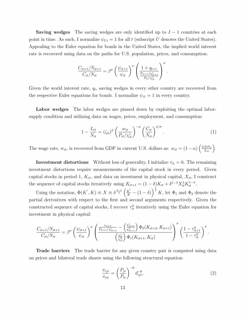
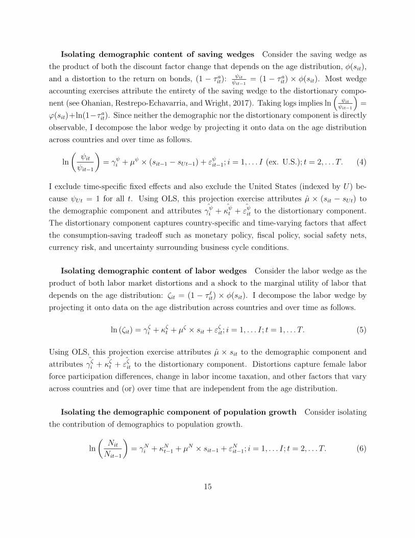
Empirical relationship between demographics and wedges Table 2 reports the

estimated elasticities of each wedge with respect to the working age share. The saving wedge

has a positive elasticity, while both the labor wedge and population growth have negative

elasticities. The R2 is quite low for the saving wedge, reflecting the fact that the wedges

are fairly noisy over time (see Figure 2a), whereas working age shares are fairly smooth.

Hence, the positive coefficient is capturing the long-run behavior. For instance, China’s

saving wedge is uniformly higher than that of the U.S. after 1990, the same period in which

China’s working age share was larger and growing rapidly. The labor wedges in all countries

tend to decline over time relatively smoothly (see Figure 2b); the R2 for the labor wedge

regression is over 75 percent.

Table 2: Estimated elasticity of wedges w.r.t. the working age share

Left-hand side variable Coefficient on Point estimate (S.E.) R2

(wedge) working age share

Saving wedge(

ψtψt−1

)µψ 0.147 (0.044) 0.013

Labor wedge (ζt) µζ -1.740 (0.060) 0.759

Population growth(

NtNt−1

)µN -0.044 (0.002) 0.787

Notes: The estimates are based on OLS regressions using equation (6)-(5).

Figure 2: Calibrated wedges

(a) Log saving wedge: ln(ψit+1

ψit

)

1970 1975 1980 1985 1990 1995 2000 2005 2010 2015

-0.8

-0.6

-0.4

-0.2

0

0.2

0.4

CHN

USA

(b) Log labor wedge: ln (ζit)

1970 1975 1980 1985 1990 1995 2000 2005 2010 2015

-0.2

0

0.2

0.4

0.6

0.8

1

1.2

CHN

USA

Notes: The U.S. saving wedge is normalized to 1 in every period.

16

4 Counterfactual analysis

To quantify the importance of demographics, I exploit the estimates from equations (4)-(6)

to construct counterfactual processes for the wedges by removing variation stemming from

the demographic component. Given the counterfactual processes for the wedges, I compute

the dynamic equilibrium under perfect foresight from 1970-2060. Appendix E provides the

details of the algorithm for solving for the transition, which builds on Sposi (2012) and

Ravikumar, Santacreu, and Sposi (2017).

4.1 Freezing each country’s working age share as of 1970

In order to quantify the importance of differential changes in working age shares across coun-

tries, this counterfactual assumes that the working age share of the population is constant

from 1970-2060. I construct counterfactual sequences for saving wedges, labor wedges, and

population by removing the variation that stems from the working age share, but allowing

the distortionary component to vary over time, as follows.

ψsi70it =

ψit, t = 1970

exp

(γψi + µψ × (si1970 − sU1970) + εψit

)× ψsi70it−1, t ≥ 1971

, (7a)

ζsi70it = exp(γζi + κζt + µζ × si1970 + εζit

), t ≥ 1970. (7b)

N si70it =

Nit, t = 1970

exp(γNi + κNt + µN × si1970 + εNit

)×N si70

it−1, t ≥ 1971, (7c)

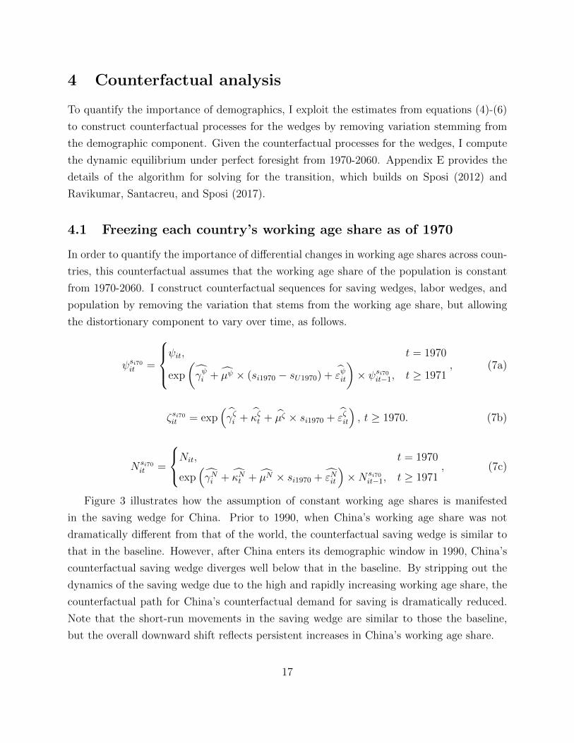
Figure 3 illustrates how the assumption of constant working age shares is manifested

in the saving wedge for China. Prior to 1990, when China’s working age share was not

dramatically different from that of the world, the counterfactual saving wedge is similar to

that in the baseline. However, after China enters its demographic window in 1990, China’s

counterfactual saving wedge diverges well below that in the baseline. By stripping out the

dynamics of the saving wedge due to the high and rapidly increasing working age share, the

counterfactual path for China’s counterfactual demand for saving is dramatically reduced.

Note that the short-run movements in the saving wedge are similar to those the baseline,

but the overall downward shift reflects persistent increases in China’s working age share.

17

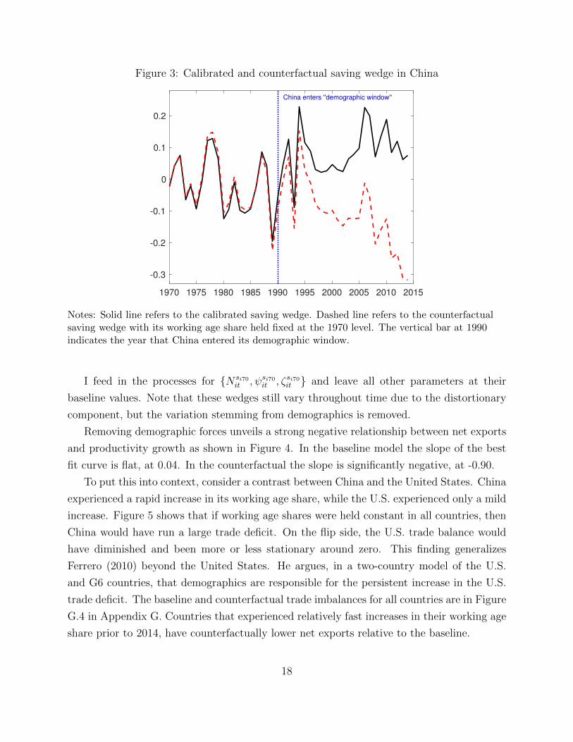
Figure 3: Calibrated and counterfactual saving wedge in China

1970 1975 1980 1985 1990 1995 2000 2005 2010 2015

-0.3

-0.2

-0.1

0

0.1

0.2

China enters ''demographic window''

Notes: Solid line refers to the calibrated saving wedge. Dashed line refers to the counterfactualsaving wedge with its working age share held fixed at the 1970 level. The vertical bar at 1990indicates the year that China entered its demographic window.

I feed in the processes for {N si70it , ψsi70it , ζsi70it } and leave all other parameters at their

baseline values. Note that these wedges still vary throughout time due to the distortionary

component, but the variation stemming from demographics is removed.

Removing demographic forces unveils a strong negative relationship between net exports

and productivity growth as shown in Figure 4. In the baseline model the slope of the best

fit curve is flat, at 0.04. In the counterfactual the slope is significantly negative, at -0.90.

To put this into context, consider a contrast between China and the United States. China

experienced a rapid increase in its working age share, while the U.S. experienced only a mild

increase. Figure 5 shows that if working age shares were held constant in all countries, then

China would have run a large trade deficit. On the flip side, the U.S. trade balance would

have diminished and been more or less stationary around zero. This finding generalizes

Ferrero (2010) beyond the United States. He argues, in a two-country model of the U.S.

and G6 countries, that demographics are responsible for the persistent increase in the U.S.

trade deficit. The baseline and counterfactual trade imbalances for all countries are in Figure

G.4 in Appendix G. Countries that experienced relatively fast increases in their working age

share prior to 2014, have counterfactually lower net exports relative to the baseline.

18

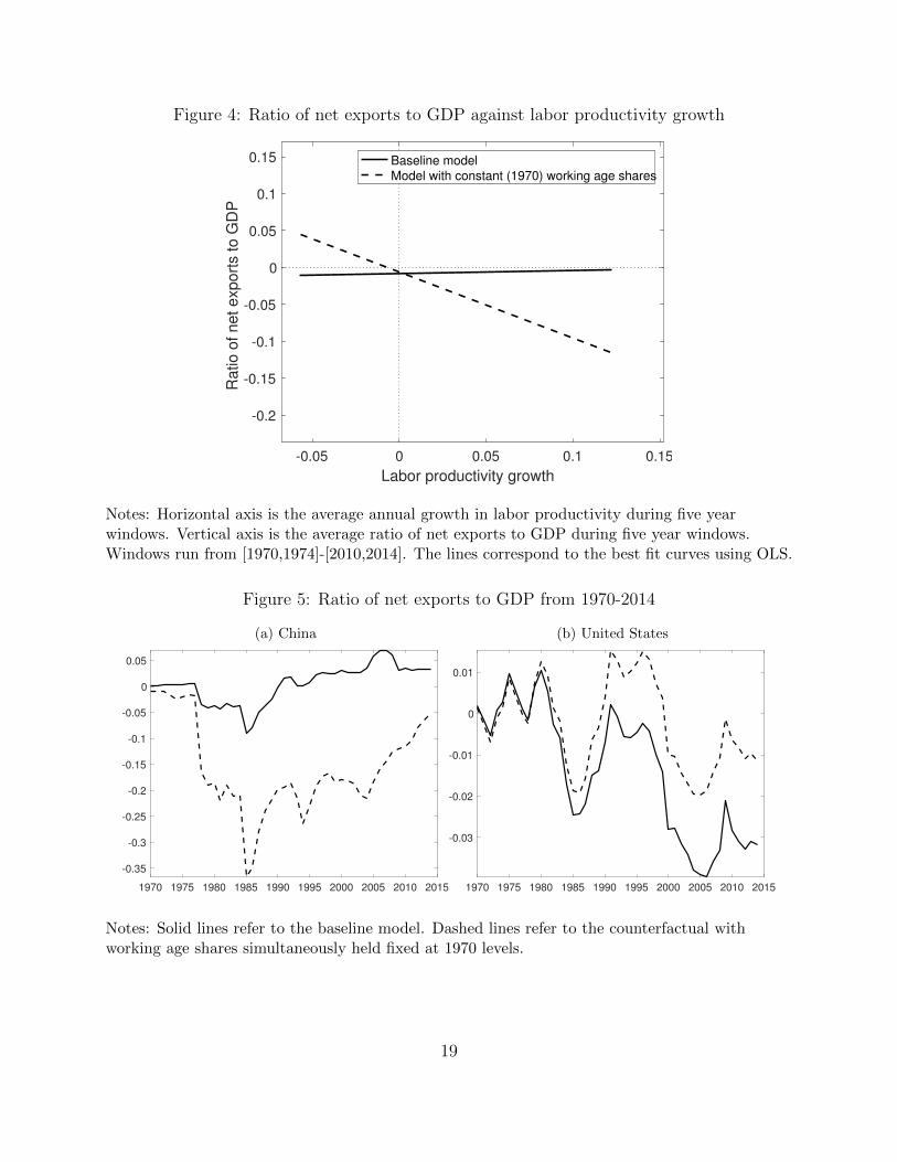
Figure 4: Ratio of net exports to GDP against labor productivity growth

-0.05 0 0.05 0.1 0.15

Labor productivity growth

-0.2

-0.15

-0.1

-0.05

0

0.05

0.1

0.15

Ra

tio

of

ne

t e

xp

ort

s t

o G

DP

Baseline model

Model with constant (1970) working age shares

Notes: Horizontal axis is the average annual growth in labor productivity during five yearwindows. Vertical axis is the average ratio of net exports to GDP during five year windows.Windows run from [1970,1974]-[2010,2014]. The lines correspond to the best fit curves using OLS.

Figure 5: Ratio of net exports to GDP from 1970-2014

(a) China

1970 1975 1980 1985 1990 1995 2000 2005 2010 2015

-0.35

-0.3

-0.25

-0.2

-0.15

-0.1

-0.05

0

0.05

(b) United States

1970 1975 1980 1985 1990 1995 2000 2005 2010 2015

-0.03

-0.02

-0.01

0

0.01

Notes: Solid lines refer to the baseline model. Dashed lines refer to the counterfactual withworking age shares simultaneously held fixed at 1970 levels.

19

Consider the ratio of net exports to GDP as the product of (i) the ratio of net exports

to trade (intertemporal margin) and (ii) the ratio of trade to GDP (intratemporal margin):

EXP − IMP

GDP=

(EXP − IMP

EXP + IMP

)×(EXP + IMP

GDP

)(8)

In Figure 6a, China’s counterfactual ratio of net exports to trade is uniformly lower

compared to the baseline. The ratio of trade to GDP (Figure 6b) is slightly higher, amplifying

the contribution of the ratio of net exports to trade to the ratio of net exports to GDP.

Figure 6: Ratio of net exports to trade and ratio of trade to GDP from 1970-2014

(a) China: Ratio of net exports to trade

1970 1975 1980 1985 1990 1995 2000 2005 2010 2015

-0.8

-0.6

-0.4

-0.2

0

0.2

0.4

(b) United States: Ratio of net exports to trade

1970 1975 1980 1985 1990 1995 2000 2005 2010 2015

-0.25

-0.2

-0.15

-0.1

-0.05

0

0.05

0.1

(c) China: Ratio of trade to GDP

1970 1975 1980 1985 1990 1995 2000 2005 2010 2015

0.05

0.1

0.15

0.2

0.25

0.3

0.35

0.4

0.45

(d) United States: Ratio of trade to GDP

1970 1975 1980 1985 1990 1995 2000 2005 2010 2015

0.08

0.1

0.12

0.14

0.16

0.18

Notes: Solid lines refer to the baseline model. Dashed lines refer to the counterfactual withworking age shares simultaneously held fixed at 1970 levels.

20

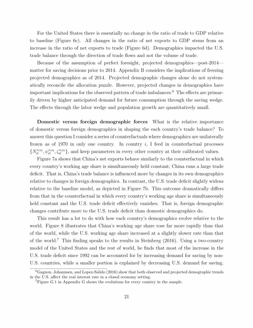
For the United States there is essentially no change in the ratio of trade to GDP relative

to baseline (Figure 6c). All changes in the ratio of net exports to GDP stems from an

increase in the ratio of net exports to trade (Figure 6d). Demographics impacted the U.S.

trade balance through the direction of trade flows and not the volume of trade.

Because of the assumption of perfect foresight, projected demographics—post-2014—

matter for saving decisions prior to 2014. Appendix B considers the implications of freezing

projected demographics as of 2014. Projected demographic changes alone do not system-

atically reconcile the allocation puzzle. However, projected changes in demographics have

important implications for the observed pattern of trade imbalances.6 The effects are primar-

ily driven by higher anticipated demand for future consumption through the saving wedge.

The effects through the labor wedge and population growth are quantitatively small.

Domestic versus foreign demographic forces What is the relative importance

of domestic versus foreign demographics in shaping the each country’s trade balance? To

answer this question I consider a series of counterfactuals where demographics are unilaterally

frozen as of 1970 in only one country. In country i, I feed in counterfactual processes

{N si70it , ψsi70it , ζsi70it }, and keep parameters in every other country at their calibrated values.

Figure 7a shows that China’s net exports behave similarly to the counterfactual in which

every country’s working age share is simultaneously held constant; China runs a large trade

deficit. That is, China’s trade balance is influenced more by changes in its own demographics

relative to changes in foreign demographics. In contrast, the U.S. trade deficit slightly widens

relative to the baseline model, as depicted in Figure 7b. This outcome dramatically differs

from that in the counterfactual in which every country’s working age share is simultaneously

held constant and the U.S. trade deficit effectively vanishes. That is, foreign demographic

changes contribute more to the U.S. trade deficit than domestic demographics do.

This result has a lot to do with how each country’s demographics evolve relative to the

world. Figure 8 illustrates that China’s working age share rose far more rapidly than that

of the world, while the U.S. working age share increased at a slightly slower rate than that

of the world.7 This finding speaks to the results in Steinberg (2016). Using a two-country

model of the United States and the rest of world, he finds that most of the increase in the

U.S. trade deficit since 1992 can be accounted for by increasing demand for saving by non-

U.S. countries, while a smaller portion is explained by decreasing U.S. demand for saving.

6Gagnon, Johannsen, and Lopez-Salido (2016) show that both observed and projected demographic trendsin the U.S. affect the real interest rate in a closed economy setting.

7Figure G.1 in Appendix G shows the evolutions for every country in the sample.

21

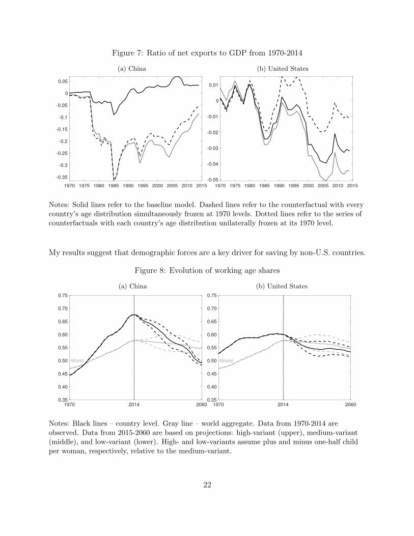
Figure 7: Ratio of net exports to GDP from 1970-2014

(a) China

1970 1975 1980 1985 1990 1995 2000 2005 2010 2015

-0.35

-0.3

-0.25

-0.2

-0.15

-0.1

-0.05

0

0.05

(b) United States

1970 1975 1980 1985 1990 1995 2000 2005 2010 2015

-0.05

-0.04

-0.03

-0.02

-0.01

0

0.01

Notes: Solid lines refer to the baseline model. Dashed lines refer to the counterfactual with everycountry’s age distribution simultaneously frozen at 1970 levels. Dotted lines refer to the series ofcounterfactuals with each country’s age distribution unilaterally frozen at its 1970 level.

My results suggest that demographic forces are a key driver for saving by non-U.S. countries.

Figure 8: Evolution of working age shares

(a) China

1970 2014 2060

0.35

0.40

0.45

0.50

0.55

0.60

0.65

0.70

0.75

World

(b) United States

1970 2014 2060

0.35

0.40

0.45

0.50

0.55

0.60

0.65

0.70

0.75

World

Notes: Black lines – country level. Gray line – world aggregate. Data from 1970-2014 areobserved. Data from 2015-2060 are based on projections: high-variant (upper), medium-variant(middle), and low-variant (lower). High- and low-variants assume plus and minus one-half childper woman, respectively, relative to the medium-variant.

22

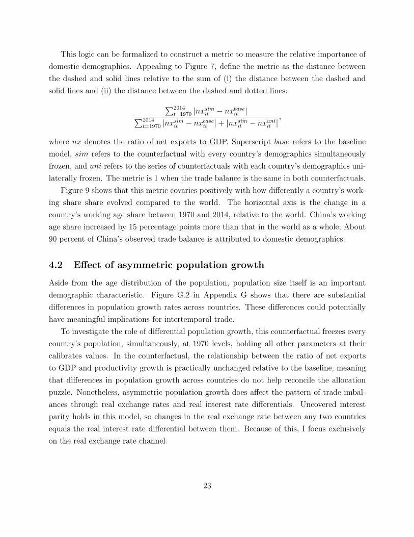
This logic can be formalized to construct a metric to measure the relative importance of

domestic demographics. Appealing to Figure 7, define the metric as the distance between

the dashed and solid lines relative to the sum of (i) the distance between the dashed and

solid lines and (ii) the distance between the dashed and dotted lines:∑2014t=1970 |nxsimit − nxbaseit |∑2014

t=1970 |nxsimit − nxbaseit |+ |nxsimit − nxuniit |,

where nx denotes the ratio of net exports to GDP. Superscript base refers to the baseline

model, sim refers to the counterfactual with every country’s demographics simultaneously

frozen, and uni refers to the series of counterfactuals with each country’s demographics uni-

laterally frozen. The metric is 1 when the trade balance is the same in both counterfactuals.

Figure 9 shows that this metric covaries positively with how differently a country’s work-

ing share share evolved compared to the world. The horizontal axis is the change in a

country’s working age share between 1970 and 2014, relative to the world. China’s working

age share increased by 15 percentage points more than that in the world as a whole; About

90 percent of China’s observed trade balance is attributed to domestic demographics.

4.2 Effect of asymmetric population growth

Aside from the age distribution of the population, population size itself is an important

demographic characteristic. Figure G.2 in Appendix G shows that there are substantial

differences in population growth rates across countries. These differences could potentially

have meaningful implications for intertemporal trade.

To investigate the role of differential population growth, this counterfactual freezes every

country’s population, simultaneously, at 1970 levels, holding all other parameters at their

calibrates values. In the counterfactual, the relationship between the ratio of net exports

to GDP and productivity growth is practically unchanged relative to the baseline, meaning

that differences in population growth across countries do not help reconcile the allocation

puzzle. Nonetheless, asymmetric population growth does affect the pattern of trade imbal-

ances through real exchange rates and real interest rate differentials. Uncovered interest

parity holds in this model, so changes in the real exchange rate between any two countries

equals the real interest rate differential between them. Because of this, I focus exclusively

on the real exchange rate channel.

23

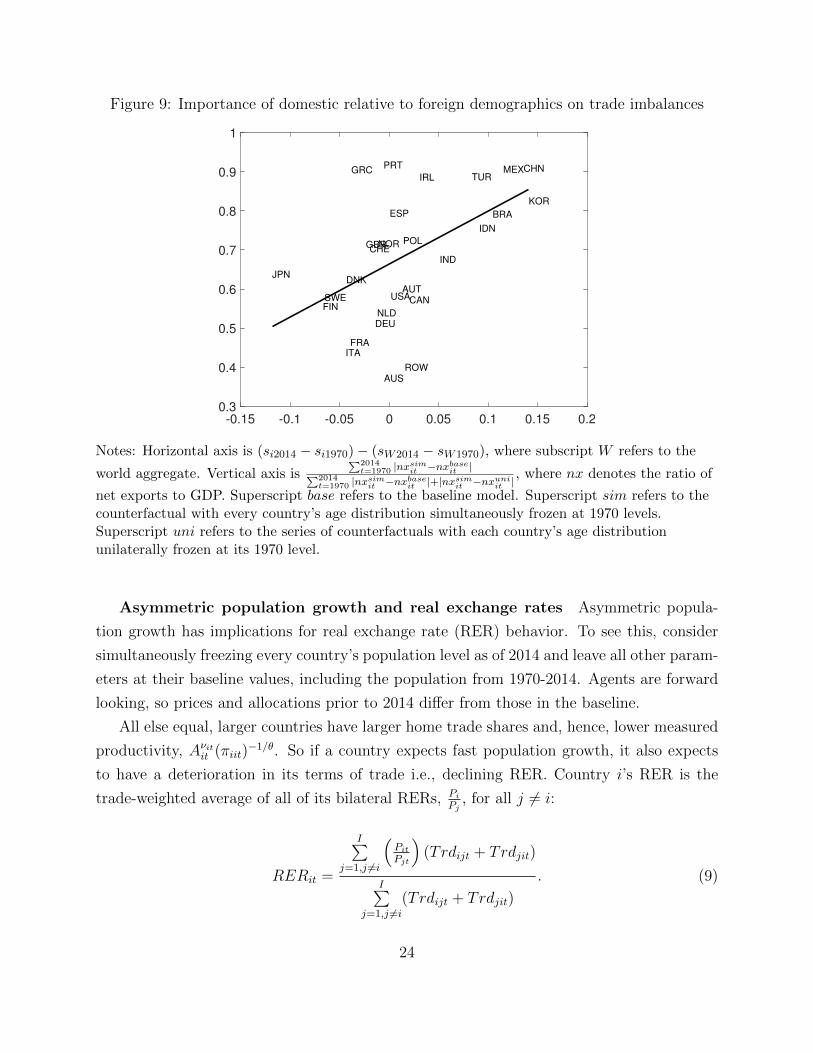
Figure 9: Importance of domestic relative to foreign demographics on trade imbalances

-0.15 -0.1 -0.05 0 0.05 0.1 0.15 0.20.3

0.4

0.5

0.6

0.7

0.8

0.9

1

AUS

AUT

BRA

CAN

CHN

DNK

FIN

FRA

DEU

GRC

IND

IDN

IRL

ITA

JPN

KOR

MEX

NLD

NOR POL

PRT

ESP

SWE

CHE

TUR

GBR

USA

ROW

Notes: Horizontal axis is (si2014 − si1970)− (sW2014 − sW1970), where subscript W refers to the

world aggregate. Vertical axis is∑2014t=1970 |nxsimit −nxbaseit |∑2014

t=1970 |nxsimit −nxbaseit |+|nxsimit −nxuniit |, where nx denotes the ratio of

net exports to GDP. Superscript base refers to the baseline model. Superscript sim refers to thecounterfactual with every country’s age distribution simultaneously frozen at 1970 levels.Superscript uni refers to the series of counterfactuals with each country’s age distributionunilaterally frozen at its 1970 level.

Asymmetric population growth and real exchange rates Asymmetric popula-

tion growth has implications for real exchange rate (RER) behavior. To see this, consider

simultaneously freezing every country’s population level as of 2014 and leave all other param-

eters at their baseline values, including the population from 1970-2014. Agents are forward

looking, so prices and allocations prior to 2014 differ from those in the baseline.

All else equal, larger countries have larger home trade shares and, hence, lower measured

productivity, Aνitit (πiit)−1/θ. So if a country expects fast population growth, it also expects

to have a deterioration in its terms of trade i.e., declining RER. Country i’s RER is the

trade-weighted average of all of its bilateral RERs, PiPj

, for all j 6= i:

RERit =

I∑j=1,j 6=i

(PitPjt

)(Trdijt + Trdjit)

I∑j=1,j 6=i

(Trdijt + Trdjit)

. (9)

24

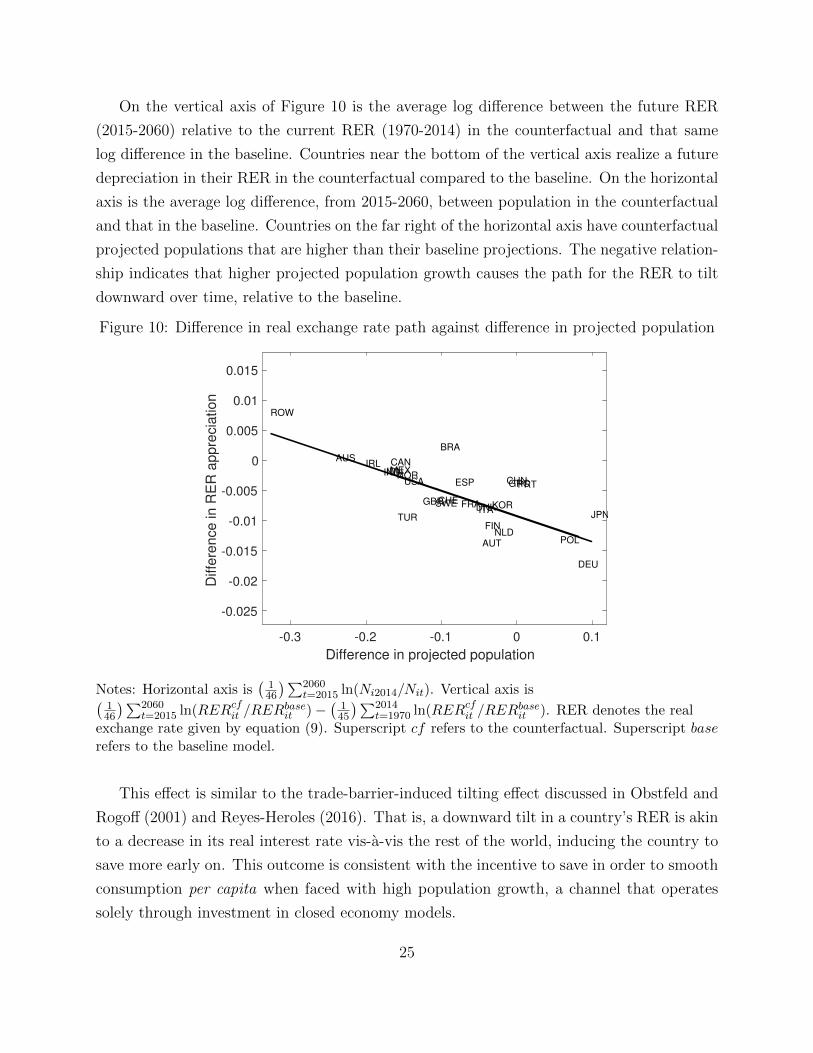
On the vertical axis of Figure 10 is the average log difference between the future RER

(2015-2060) relative to the current RER (1970-2014) in the counterfactual and that same

log difference in the baseline. Countries near the bottom of the vertical axis realize a future

depreciation in their RER in the counterfactual compared to the baseline. On the horizontal

axis is the average log difference, from 2015-2060, between population in the counterfactual

and that in the baseline. Countries on the far right of the horizontal axis have counterfactual

projected populations that are higher than their baseline projections. The negative relation-

ship indicates that higher projected population growth causes the path for the RER to tilt

downward over time, relative to the baseline.

Figure 10: Difference in real exchange rate path against difference in projected population

-0.3 -0.2 -0.1 0 0.1

Difference in projected population

-0.025

-0.02

-0.015

-0.01

-0.005

0

0.005

0.01

0.015

Diffe

ren

ce

in

RE

R a

pp

recia

tio

n

AUS

AUT

BRA

CAN

CHN

DNK

FIN

FRA

DEU

GRCINDIDN

IRL

ITAJPN

KOR

MEX

NLD

NOR

POL

PRTESP

SWECHE

TUR

GBR

USA

ROW

Notes: Horizontal axis is(

146

)∑2060t=2015 ln(Ni2014/Nit). Vertical axis is(

146

)∑2060t=2015 ln(RERcfit /RER

baseit )−

(145

)∑2014t=1970 ln(RERcfit /RER

baseit ). RER denotes the real

exchange rate given by equation (9). Superscript cf refers to the counterfactual. Superscript baserefers to the baseline model.

This effect is similar to the trade-barrier-induced tilting effect discussed in Obstfeld and

Rogoff (2001) and Reyes-Heroles (2016). That is, a downward tilt in a country’s RER is akin

to a decrease in its real interest rate vis-a-vis the rest of the world, inducing the country to

save more early on. This outcome is consistent with the incentive to save in order to smooth

consumption per capita when faced with high population growth, a channel that operates

solely through investment in closed economy models.

25

4.3 Trade barriers as a driver of imbalances

Trade barriers are directly related to bilateral trade flows and, hence, have immediate impli-

cations for the trade balance. I decompose the bilateral trade barriers into a trend component

and a bilateral distortionary component as follows

ln(dijt − 1) = ln(dt − 1) + εdijt.

I decompose (d− 1)—the portion that melts away—as opposed to d. The trend component

of trade barriers is simply the geometric mean of all bilateral trade barriers:

dt = 1 + exp

I∑i=1

I∑j=1j 6=i

ln(dijt − 1)

.

The estimated trend component, dt, steadily declined from 4.5 in 1970 to 2.6 in 2014.

This decline captures global reductions shipping costs as well as tariff reductions. The

distortionary component captures bilateral changes in trade barriers that are specific to

bilateral trading pairs beyond the trend component.

Freezing the bilateral distortions I quantify the effect of changes in the distor-

tionary component by constructing a counterfactual path for bilateral trade barriers with

the distortionary component held constant at 1970 values, but allow the trend component

to vary over time:

dεdij70t = 1 +

(dt − 1)× exp

(εdij1970

). (10)

In this counterfactual there is a strong positive relationship between the ratio of net

exports to GDP and labor productivity growth: The elasticity is 0.80, compared to 0.04 in

the baseline. Controlling for changes in the distortionary component of trade barriers makes

the allocation puzzle even more puzzling.

That is not to say that asymmetries in trade barriers are unimportant in driving each

country’s trade balance. For instance, Figure 11 suggests that the U.S. trade distortions

played a role in shaping the U.S. trade imbalance. The late 1970s and early 2000s are

precisely the periods that the average U.S. export distortion rose, and the counterfactual

U.S. net exports exceeded the observed (baseline) U.S. net exports (dotted line compared to

solid line).

26

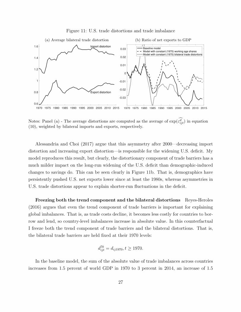
Figure 11: U.S. trade distortions and trade imbalance

(a) Average bilateral trade distortion

1970 1975 1980 1985 1990 1995 2000 2005 2010 2015

0.6

0.8

1

1.2

1.4

1.6 Import distortion

Export distortion

(b) Ratio of net exports to GDP

1970 1975 1980 1985 1990 1995 2000 2005 2010 2015

-0.03

-0.02

-0.01

0

0.01

0.02

0.03 Baseline model

Model with constant (1970) working age shares

Model with constant (1970) bilateral trade distortions

Notes: Panel (a) - The average distortions are computed as the average of exp(εdijt) in equation(10), weighted by bilateral imports and exports, respectively.

Alessandria and Choi (2017) argue that this asymmetry after 2000—decreasing import

distortion and increasing export distortion—is responsible for the widening U.S. deficit. My

model reproduces this result, but clearly, the distortionary component of trade barriers has a

much milder impact on the long-run widening of the U.S. deficit than demographic-induced

changes to savings do. This can be seen clearly in Figure 11b. That is, demographics have

persistently pushed U.S. net exports lower since at least the 1980s, whereas asymmetries in

U.S. trade distortions appear to explain shorter-run fluctuations in the deficit.

Freezing both the trend component and the bilateral distortions Reyes-Heroles

(2016) argues that even the trend component of trade barriers is important for explaining

global imbalances. That is, as trade costs decline, it becomes less costly for countries to bor-

row and lend, so country-level imbalances increase in absolute value. In this counterfactual

I freeze both the trend component of trade barriers and the bilateral distortions. That is,

the bilateral trade barriers are held fixed at their 1970 levels:

d70ijt = dij1970, t ≥ 1970.

In the baseline model, the sum of the absolute value of trade imbalances across countries

increases from 1.5 percent of world GDP in 1970 to 3 percent in 2014, an increase of 1.5

27

percentage points. In the counterfactual with the working age share held fixed this ratio

increases by 2.3 percentage points. In the counterfactual with trade barriers held fixed this

ratio decreases by 2.1 percentage points (from 5.3 percent to 3.2 percent). As such, variation

in the working age share does not help explain the overall increase in the magnitude of global

imbalances over time, while variation in trade barriers does.

4.4 Investment and labor market distortions

Existing literature has emphasized distortions to investment and labor markets as important

drivers of imbalances. I study each of these in the context of the allocation puzzle.

Investment distortions Intertemporal choices are affected by investment distortions,

which directly affect real rates of return and can have profound implications for capital flows

and trade imbalances. These distortions capture financial frictions pertaining to investment,

such as those in Buera and Shin (2017), as well as institutional problems that discourage

investment, such as those discussed in Aguiar and Amador (2011). I consider a counterfactual

in which the investment distortions are held fixed at 1970 levels in every country:

τ k,70it = τ ki1970, t ≥ 1970.

In this counterfactual the elasticity of the ratio of net exports to GDP with respect to

labor productivity growth is -0.16, compared to 0.04 in the baseline. Therefore, removing

variation in investment distortions partly alleviates the allocation puzzle but does so to a

far lesser extent than removing variation in working age shares.

Labor market distortions The calibrated labor wedges contain a demographic com-

ponent and a distortionary component. This counterfactual holds fixed the variation stem-

ming from the distortionary component as of 1970. The reduced form nature of the decom-

position implies that these distortions are captured by the time-fixed effect and the residual

in equation (5). The fixed effects capture common global factors that affect labor market

dynamics, such as technological change and large scale GATT/WTO reforms. The resid-

ual captures country-specific distortions that vary over time, such as fiscal policy and other

factors emphasized by Ohanian, Restrepo-Echavarria, and Wright (2017). As such, I set

28

κζt = κζ1970 and εζit = εζi1970 and compute counterfactual process for the labor wedges.

ζεζi1970it = exp

(γζi + κζ1970 + µζ × sit + εζi1970

), t ≥ 1970

In this counterfactual the elasticity of the ratio of net exports to GDP with respect

to labor productivity growth is 0.15. This elasticity is greater than that in the baseline,

implying that labor market distortions do not systematically explain the allocation puzzle,

but actually make it more puzzling.

4.5 Summary

Table 3 reports the elasticity between the ratio of net exports to GDP and productivity

growth for the baseline and counterfactual specifications. Changes in demographics are by

far the most important for reconciling the allocation puzzle. Investment distortions partially

alleviate the puzzle, but to a far less degree than demographics. Neither bilateral trade

distortions nor labor market distortions help reconcile the allocation puzzle.

This is not to say that trade barriers and labor market distortions are irrelevant for

trade imbalances. Bilateral trade distortions help shape short-run behavior of country-level

imbalances, but cannot account for long-run persistence. The continual decline in trade

barriers across the world do help account for the absolute rise in global imbalances, but

cannot account for the pattern of imbalances across countries.

Table 3: Elasticity between ratio of net exports to GDP and productivity growth

Specification ElasticityBaseline model (data) 0.04Counterfactual: Fixed working age shares −0.90Counterfactual: Fixed bilateral trade distortions +0.81Counterfactual: Fixed investment distortions −0.16Counterfactual: Fixed labor market distortions +0.15

The main findings suggest that there is an intimate relationship between changes in the

working age share and the rate of labor productivity growth. Countries that experienced fast

productivity growth, but did not run trade deficits, also tend to be countries that experienced

relatively fast increases in their working age shares. By counterfactually holding fixed the

working age share and removing demographic-induced changes to saving, the correlation

between net exports and productivity growth becomes negative.

29

Life-cycle models could generate the link between saving and productivity growth. Older

workers have higher income than young workers and also save more as they near retirement.

If worker-level earnings reflect productivity, then increases in the working age share due to

an aging population can yield higher productivity growth alongside higher saving.

5 Conclusion

The paper builds a multicountry, dynamic, Ricardian model of trade, where dynamics are

driven by international borrowing and lending and capital accumulation. Trade imbalances

arise endogenously as the result of relative shifts in technologies, in trade barriers, in factor

market distortions, and in demographics. All of the exogenous forces are calibrated using

a wedge accounting procedure so that the model rationalizes past and projected national

accounts data and bilateral trade flows across 28 countries from 1970-2060.

Demographics directly affect imbalances through the relative demand for national saving

and indirectly impact imbalances through labor supply and population growth. By counter-

factually holding fixed the working age share in each country as of 1970, a strong negative

relationship between each country’s ratio of net exports to GDP and productivity growth

emerges. In other words, demographics alleviate the allocation puzzle. Net exports respond

more to domestic demographics, relative to foreign demographics, in countries in which the

working age share evolved more differently from the world average.

Differences in population growth do not help reconcile the allocation puzzle. However,

countries with relatively fast projected population growth experience relative declines in their

real exchange rate over time and finance higher rates of consumption growth by borrowing

early and lending late. Investment distortions shed some light on the allocation puzzle, but

do so to a lesser degree than demographics. Neither labor market distortions nor trade

distortions help reconcile the puzzle.

The results in this paper allude to a relationship between productivity growth and changes

in demographics. Countries that experienced fast productivity growth, but did not run trade

deficits, tend to be the same countries that experienced relatively fast increases in their

working age shares. Digging into this relationship is beyond of the scope of this paper.

Future work should aim at developing methods that explicitly incorporate heterogeneity in

age, such as an overlapping generations environment, into a multicountry dynamic model

of trade. Such a framework can be used to more carefully study how demographics shape

productivity, comparative advantage, and trade imbalances in a unified framework.

30

References

Adao, Rodrigo, Costas Arkolakis, and Federico Esposito. 2017. “Trade, Agglomoration

Effects, and Labor Markets: Theory and Evidence.” Mimeo.

Aguiar, Mark and Manuel Amador. 2011. “Growth in the Shadow of Expropriation.” Quar-

terly Journal of Economics 126 (2):651–697.

Alessandria, George and Horag Choi. 2017. “The Dynamics of the Trade Balance and the

Real Exchange Rate: The J Curve and Trade Costs?” Mimeo.

Alfaro, Laura, Sebnem Kalemli-Ozcan, and Vadym Volosovych. 2008. “Why Doesn’t Capital

Flow From Rich to Poor Countries? An Empirical Investigation.” Review of Economics

and Statistics 90 (2):347–368.

Alvarez, Fernando. 2017. “Capital Accumulation and International Trade.” Journal of

Monetary Economics 91 (C):1–18.

Alvarez, Fernando and Robert E. Lucas. 2007. “General Equilibrium Analysis of the Eaton-

Kortum Model of International Trade.” Journal of Monetary Economics 54 (6):1726–1768.

Blanchard, Olivier J. 1985. “Debt, Deficits, and Finite Horizons.” Journal of Political

Economy 93 (2):223–247.

Buera, Francisco J. and Yongseok Shin. 2017. “Productivity Growth and Capital Flows:

The Dynamics of Reforms.” American Economic Journal: Macroeconomics 9 (3):147–85.

Caliendo, Lorenzo, Maximiliano Dvorkin, and Fernando Parro. 2015. “Trade and Labor

Market Dynamics.” Working Paper 21149, National Bureau of Economic Research.

Carroll, Christopher D., Jody Overland, and David N. Weil. 2000. “Saving and Growth with

Habit Formation.” American Economic Review 90 (3):341–355.

Caselli, Francesco and James Feyrer. 2007. “The Marginal Product of Capital.” Quarterly

Journal of Economics 122 (2):535–568.

Chari, V.V., Patrick J. Kehoe, and Ellen R. McGrattan. 2007. “Business Cycle Accounting.”

Econometrica 75 (3):781–836.

31

Eaton, Jonathan, Samuel Kortum, Brent Neiman, and John Romalis. 2016. “Trade and the

Global Recession.” American Economic Review 106 (11):3401–3438.

Feenstra, Robert C., Robert Inklaar, and Marcel P. Timmer. 2015. “The Next Generation

of the Penn World Table.” American Economic Review 105 (10):3150–3182.

Ferrero, Andrea. 2010. “A Structural Decomposition of the U.S. Trade Balance: Productiv-

ity, Demographics and Fiscal Policy.” Journal of Monetary Economics 57 (4):478–490.

Gagnon, Etienne, Benjamin K. Johannsen, and J. David Lopez-Salido. 2016. “Understanding

the New Normal : The Role of Demographics.” Finance and Economics Discussion Series

2016-080, Board of Governors of the Federal Reserve System (U.S.).

Gollin, Douglas. 2002. “Getting Income Shares Right.” Journal of Political Economy

110 (2):458–474.

Gourinchas, Pierre-Olivier and Olivier Jeanne. 2013. “Capital Flows to Developing Coun-

tries: The Allocation Puzzle.” Review of Economic Studies 80 (4):1422–1458.

Higgins, Matthew. 1998. “Demography, National Savings, and International Capital Flows.”

International Economic Review 39 (2):343–369.

Imorohoglu, Ayse and Kai Zhao. 2017a. “The Chinese Saving Rate: Long-Term Care Risks,

Family Insurance, and Demographics.” Mimeo.

———. 2017b. “Household Saving, Financial Constraints, and the Current Account in

China.” Mimeo.

Krueger, Dirk and Alexander Ludwig. 2007. “On the Consequences of Demographic Change

for Rates of Returns to Capital, and the Distribution of Wealth and Welfare.” Journal of

Monetary Economics 54 (1):49–87.

Lucas, Robert E. 1990. “Why Doesn’t Capital Flow from Rich to Poor Countries?” American

Economic Review 80 (2):92–96.

Maliar, Lilia, Serguei Maliar, John Taylor, and Inna Tsener. 2015. “A Tractable Framework

for Analyzing a Class of Nonstationary Markov Models.” Working Paper 21155, National

Bureau of Economic Research.

32

Obstfeld, Maurice and Kenneth Rogoff. 2001. The Six Major Puzzles in International

Macroeconomics: Is there a Common Cause? Cambridge, MA: MIT Press, 339–390.

Ohanian, Lee E., Paulina Restrepo-Echavarria, and Mark L. J. Wright. 2017. “Bad Invest-

ments and Missed Opportunities? Postwar Capital Flows to Asia and Latin America.”

Working Papers 2014-038C, Federal Reserve Bank of St. Louis.

Organization for Economic Cooperation and Development. 2014. “Long-Term Baseline Pro-

jections, No. 95 (Edition 2014).” Tech. rep. URL /content/data/data-00690-en.

Peterman, William B. 2016. “Reconciling Micro And Macro Estimates Of The Frisch Labor

Supply Elasticity.” Economic Inquiry 54 (1):100–120.

Prasad, Eswar S., Raghuram G. Rajan, and Arvind Subramanian. 2007. “Foreign Capital

and Economic Growth.” Brookings Papers on Economic Activity 1:153–230.

Ravikumar, B., Ana Maria Santacreu, and Michael Sposi. 2017. “Capital Accumulation and

Dynamic Gains from Trade.” Working Papers 2017-05, Federal Reserve Bank of St. Louis.

Reyes-Heroles, Ricardo. 2016. “The Role of Trade Costs in the Surge of Trade Imbalances.”

Mimeo.

Simonovska, Ina and Michael E. Waugh. 2014. “The Elasticity of Trade: Estimates and

Evidence.” Journal of International Economics 92 (1):34–50.

Song, Zheng, Kjetil Storesletten, and Fabrizio Zilibotti. 2011. “Growing Like China.” Amer-

ican Economic Review 101 (1):196–233.

Sposi, Michael. 2012. “Evolving Comparative Advantage, Structural Change, and the Com-

position of Trade.” Mimeo, University of Iowa.

Steinberg, Joseph B. 2016. “On the Source of U.S. Trade Deficits: Global Saving Glut or

Domestic Saving Draught?” Mimeo.

Timmer, Marcel P., Erik Dietzenbacher, Bart Los, Robert Stehrer, and Gaaitzen J. de Vries.

2015. “An Illustrated User Guide to the World Input-Output Database: the Case of Global

Automobile Production.” Review of International Economics 23 (3):398–411.

United Nations. 2015. “World Population Prospects: The 2015 Revision, Key Findings

and Advance Tables.” Working Paper ESA/P/WP.241, United Nations, Department of

Economic and Social Affairs, Population Division.

33

Wei, Shang-Jin and Xiaobo Zhang. 2011. “The Competitive Saving Motive: Evidence from

Rising Sex Ratios and Savings Rates in China.” Journal of Political Economy 119 (3):511–

564.

Yang, Dennis Tao, Junsen Zhang, and Shaojie Zhou. 2012. Why Are Saving Rates So High

in China? University of Chicago Press, 249–278.

Zylkin, Thomas. 2016. “Feeding China’s Rise: The Growth Effects of Trading with China,

1993-2011.” mimeo.

34

A Microfounding the wedges

Imagine data being generated by a small open economy with overlapping generations (OLG).

The econometrician views the world through the lens of a representative household and only

observes aggregate consumption, aggregate labor supply, prices, and the age distribution.

This example shows how the econometrician can calibrate preferences for the representative

household such that (i) the representative household’s decisions yield the same aggregate

outcomes as the OLG economy and (ii) variation in the wedges depends only on variation

in the age distribution.

In the OLG economy agents live for two periods. At time t a cohort arrives with Nwt

working age agents that coexist with the existing N rt retirees. Retirees disappear after one

period. Working age agents choose their labor supply. One unit of labor generates one unit

of output. There a risk-free international bond through which output can be saved.

Normalize the wage to 1 in every period, implying that the price of consumption is 1.

Take the constant world interest rate on bonds, q, as given. Agents born at time t solve

maxcwt ,c

rt+1,`

wt

{ln (cwt ) + β ln

(crt+1

)+

(1− `wt )1−1/φ

1− 1/φs.t. cwt +

crt+1

1 + q= `wt

}.

The solution is characterized (implicitly) by (1− `w) =(

`w

1+β

)φ, cw = (1− `w)1/φ, and

cr = β(1 + q)cw. While each agent’s decision is constant over time and is unaffected by

demographics, aggregate consumption, Ct = Nwt c

wt + N r

t crt , and aggregate labor supply,

Lt = Nwt `

wt , can vary over time with demographics.

Let nwt =Nwt

Ntdenote the working age share in the population at time t. Then, aggregate

consumption per capita growth and the nonemployment-population ratio, respectively, are

Ct+1/Nt+1

Ct/Nt

=

1 + nwt+1

(1−β(1+q)β(1+q)

)β(1 + q) + nwt (1− β(1 + q))

β(1 + q), (A.1)

(1− Lt

Nt

)=

((1− nwt ) +

nwt

(nwt (1− β(1 + q)) + β(1 + q))φ

)(CtNt

)φ. (A.2)

The econometrician interprets aggregate data through the lens of a representative-agent

35

model and, introduces shocks to the discount factor, ψ, and marginal utility of leisure, ζ:

max

∞∑t=1

βt−1ψtNt

ln

(CtNt

)+ ζt

(1− Lt

Nt

)1−1/φ

1− 1/φ

s.t.∞∑t=1

Ct(1 + q)t−1

=∞∑t=1

Lt(1 + q)t−1

The solution to the representative household’s problem is

Ct+1/Nt+1

Ct/Nt

=

(ψt+1

ψt

)β(1 + q), (A.3)(

1− LtNt

)= ζφt

(CtNt

)φ. (A.4)

Assume that the change in the working age share is a function of its current level:

nwt+1

nwt= ω(nwt ). (A.5)

Combining equation (A.1) with equations (A.3) and (A.5) shows that variation in the saving

wedge depends only on variation in the working age share. Similarly, combining (A.2) with

equation (A.4) shows that variation in the labor wedge depends only on variation in the

working age share. The micro-founded expressions for the calibrated wedges are

ψt+1

ψt=

1 + ω(nwt )nwt

(1−β(1+q)β(1+q)

)β(1 + q) + nwt (1− β(1 + q))

, (A.6)

ζφt =

((1− nwt ) +

nwt

(nwt (1− β(1 + q)) + β(1 + q))φ

). (A.7)

B The role of projected demographic changes

The following counterfactual exercise isolates how much of the observed trade imbalances

are due to differences in the rate that future demographics evolve. I assume that from 1970-

2014 all exogenous parameters are equal to their baseline values. Beginning in 2014, each

country’s working age share is permanently frozen. From 2015 forward each country will

face counterfactual paths for saving wedges, labor wedges, and population. All variation

in saving wedges, labor wedges, and population after 2014 can be attributed to changes in

the distortionary component, i.e., the time fixed effects and residuals in equations (6)-(5). I

36

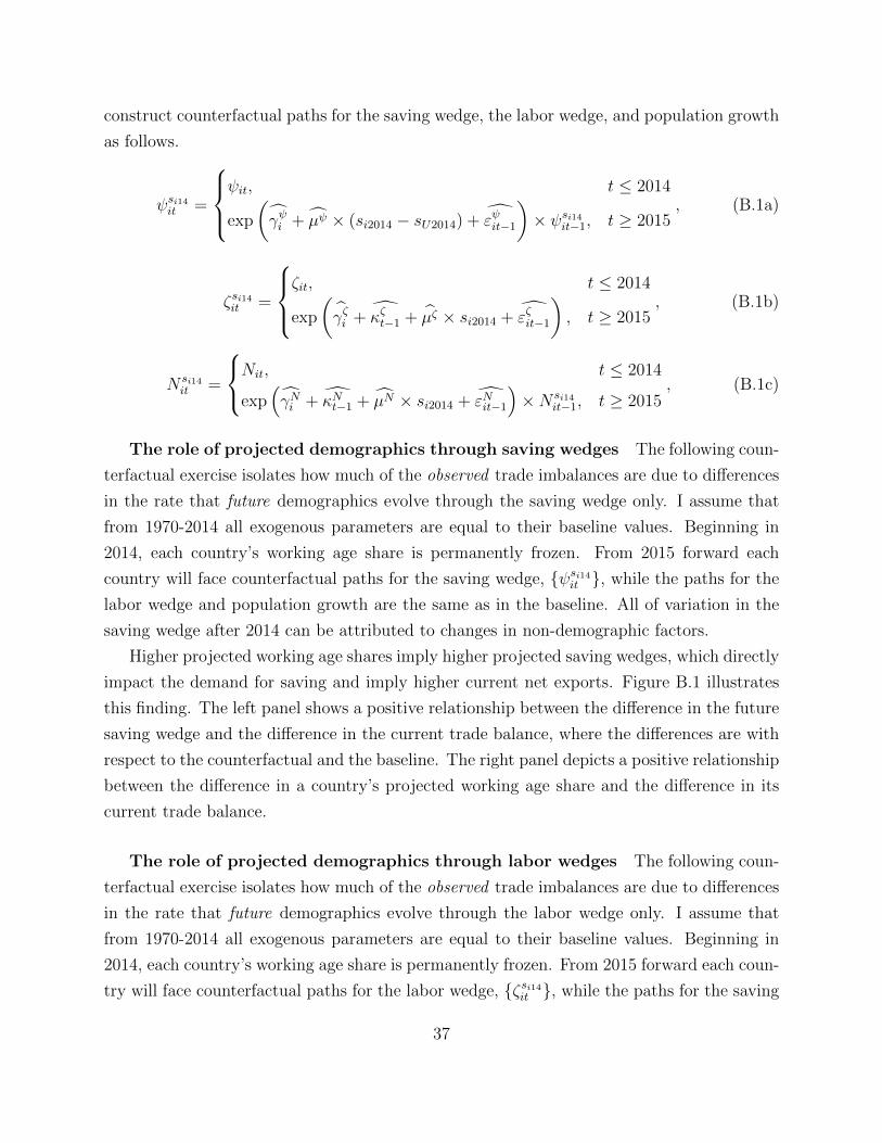
construct counterfactual paths for the saving wedge, the labor wedge, and population growth

as follows.

ψsi14it =

ψit, t ≤ 2014

exp

(γψi + µψ × (si2014 − sU2014) + εψit−1

)× ψsi14it−1, t ≥ 2015

, (B.1a)

ζsi14it =

ζit, t ≤ 2014

exp

(γζi + κζt−1 + µζ × si2014 + εζit−1

), t ≥ 2015

, (B.1b)

N si14it =

Nit, t ≤ 2014

exp(γNi + κNt−1 + µN × si2014 + εNit−1

)×N si14

it−1, t ≥ 2015, (B.1c)

The role of projected demographics through saving wedges The following coun-

terfactual exercise isolates how much of the observed trade imbalances are due to differences

in the rate that future demographics evolve through the saving wedge only. I assume that

from 1970-2014 all exogenous parameters are equal to their baseline values. Beginning in

2014, each country’s working age share is permanently frozen. From 2015 forward each

country will face counterfactual paths for the saving wedge, {ψsi14it }, while the paths for the

labor wedge and population growth are the same as in the baseline. All of variation in the

saving wedge after 2014 can be attributed to changes in non-demographic factors.

Higher projected working age shares imply higher projected saving wedges, which directly

impact the demand for saving and imply higher current net exports. Figure B.1 illustrates

this finding. The left panel shows a positive relationship between the difference in the future

saving wedge and the difference in the current trade balance, where the differences are with

respect to the counterfactual and the baseline. The right panel depicts a positive relationship

between the difference in a country’s projected working age share and the difference in its

current trade balance.

The role of projected demographics through labor wedges The following coun-

terfactual exercise isolates how much of the observed trade imbalances are due to differences

in the rate that future demographics evolve through the labor wedge only. I assume that

from 1970-2014 all exogenous parameters are equal to their baseline values. Beginning in

2014, each country’s working age share is permanently frozen. From 2015 forward each coun-

try will face counterfactual paths for the labor wedge, {ζsi14it }, while the paths for the saving

37

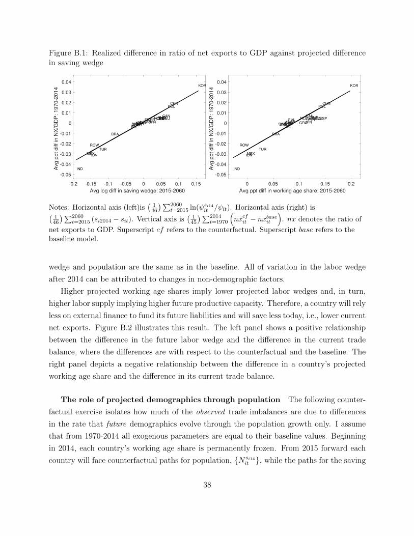
Figure B.1: Realized difference in ratio of net exports to GDP against projected differencein saving wedge

-0.2 -0.15 -0.1 -0.05 0 0.05 0.1 0.15

Avg log diff in saving wedge: 2015-2060

-0.05

-0.04

-0.03

-0.02

-0.01

0

0.01

0.02

0.03

0.04

Avg p

pt diff in

NX

/GD

P: 1970-2

014

AUS

AUT

BRA

CAN

CHN

DNK

FINFRA

DEU

GRC

IND

IDN

IRL

ITAJPN

KOR

MEX

NLD

NOR

POL

PRT ESP

SWE

CHE

TUR

GBRUSA

ROW

0 0.05 0.1 0.15 0.2

Avg ppt diff in working age share: 2015-2060

-0.05

-0.04

-0.03

-0.02

-0.01

0

0.01

0.02

0.03

0.04

Avg p

pt diff in

NX

/GD

P: 1970-2

014

AUS

AUT

BRA

CAN

CHN

DNK

FINFRA

DEU

GRC

IND

IDN

IRL

ITAJPN

KOR

MEX

NLD

NOR

POL

PRT ESP

SWE

CHE

TUR

GBRUSA

ROW

Notes: Horizontal axis (left)is(

146

)∑2060t=2015 ln(ψsi14it /ψit). Horizontal axis (right) is(

146

)∑2060t=2015 (si2014 − sit). Vertical axis is

(145

)∑2014t=1970

(nxcfit − nxbaseit

). nx denotes the ratio of

net exports to GDP. Superscript cf refers to the counterfactual. Superscript base refers to thebaseline model.

wedge and population are the same as in the baseline. All of variation in the labor wedge

after 2014 can be attributed to changes in non-demographic factors.

Higher projected working age shares imply lower projected labor wedges and, in turn,

higher labor supply implying higher future productive capacity. Therefore, a country will rely

less on external finance to fund its future liabilities and will save less today, i.e., lower current

net exports. Figure B.2 illustrates this result. The left panel shows a positive relationship

between the difference in the future labor wedge and the difference in the current trade

balance, where the differences are with respect to the counterfactual and the baseline. The

right panel depicts a negative relationship between the difference in a country’s projected

working age share and the difference in its current trade balance.

The role of projected demographics through population The following counter-

factual exercise isolates how much of the observed trade imbalances are due to differences

in the rate that future demographics evolve through the population growth only. I assume

that from 1970-2014 all exogenous parameters are equal to their baseline values. Beginning

in 2014, each country’s working age share is permanently frozen. From 2015 forward each

country will face counterfactual paths for population, {N si14it }, while the paths for the saving

38

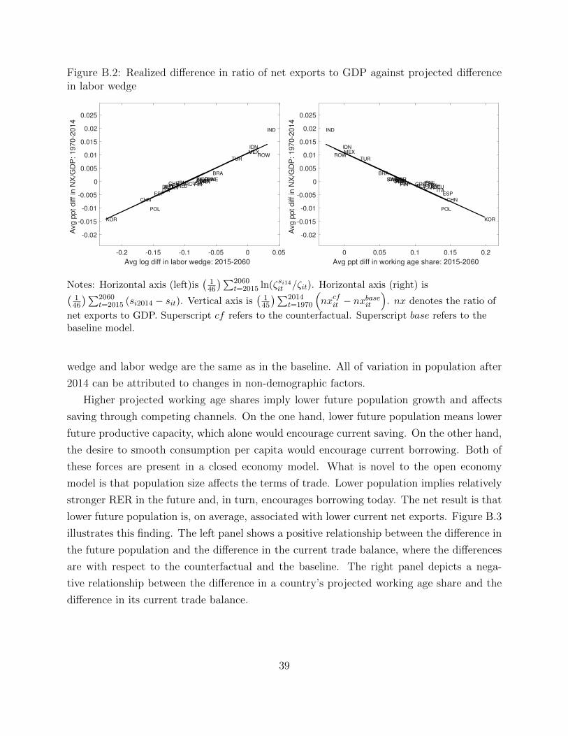
Figure B.2: Realized difference in ratio of net exports to GDP against projected differencein labor wedge

-0.2 -0.15 -0.1 -0.05 0 0.05

Avg log diff in labor wedge: 2015-2060

-0.02

-0.015

-0.01

-0.005

0

0.005

0.01

0.015

0.02

0.025

Avg p

pt diff in

NX

/GD

P: 1970-2

014

AUSAUT

BRA

CAN

CHN

DNKFIN

FRADEU

GRC

IND

IDN

IRL

ITA

JPN

KOR

MEX

NLD

NOR

POL

PRT

ESP

SWECHE

TUR

GBRUSA

ROW

0 0.05 0.1 0.15 0.2

Avg ppt diff in working age share: 2015-2060

-0.02

-0.015

-0.01

-0.005

0

0.005

0.01

0.015

0.02

0.025

Avg p

pt diff in

NX

/GD

P: 1970-2

014

AUSAUT

BRA

CAN

CHN

DNKFIN

FRADEU

GRC

IND

IDN

IRL

ITA

JPN

KOR

MEX

NLD

NOR

POL

PRT

ESP

SWECHE

TUR

GBRUSA

ROW

Notes: Horizontal axis (left)is(

146

)∑2060t=2015 ln(ζsi14it /ζit). Horizontal axis (right) is(

146

)∑2060t=2015 (si2014 − sit). Vertical axis is

(145

)∑2014t=1970

(nxcfit − nxbaseit

). nx denotes the ratio of

net exports to GDP. Superscript cf refers to the counterfactual. Superscript base refers to thebaseline model.

wedge and labor wedge are the same as in the baseline. All of variation in population after

2014 can be attributed to changes in non-demographic factors.

Higher projected working age shares imply lower future population growth and affects

saving through competing channels. On the one hand, lower future population means lower

future productive capacity, which alone would encourage current saving. On the other hand,

the desire to smooth consumption per capita would encourage current borrowing. Both of

these forces are present in a closed economy model. What is novel to the open economy

model is that population size affects the terms of trade. Lower population implies relatively

stronger RER in the future and, in turn, encourages borrowing today. The net result is that

lower future population is, on average, associated with lower current net exports. Figure B.3

illustrates this finding. The left panel shows a positive relationship between the difference in

the future population and the difference in the current trade balance, where the differences

are with respect to the counterfactual and the baseline. The right panel depicts a nega-

tive relationship between the difference in a country’s projected working age share and the

difference in its current trade balance.

39

Figure B.3: Realized difference in ratio of net exports to GDP against projected differencein population

-0.08 -0.06 -0.04 -0.02 0 0.02

Avg log diff in population: 2015-2060

-0.01

-0.005

0

0.005

0.01

Avg p

pt diff in

NX

/GD

P: 1970-2

014

AUSAUTBRACAN

CHN

DNKFIN FRADEU GRC

IND

IDNIRL

ITA JPNKOR

MEX

NLDNOR

POL

PRTESP

SWECHE

TUR

GBRUSA

ROW

0 0.05 0.1 0.15 0.2

Avg ppt diff in working age share: 2015-2060

-0.01

-0.005

0

0.005

0.01

Avg p

pt diff in

NX

/GD

P: 1970-2

014

AUS AUTBRA CAN

CHN

DNKFINFRA DEUGRC

IND

IDNIRL

ITAJPNKOR

MEX

NLDNOR

POL

PRTESP

SWE CHE

TUR

GBRUSA

ROW

Notes: Horizontal axis (left)is(

146

)∑2060t=2015 ln(N si14

it /Nit). Horizontal axis (right) is(146

)∑2060t=2015 (si2014 − sit). Vertical axis is

(145

)∑2014t=1970

(nxcfit − nxbaseit

). nx denotes the ratio of

net exports to GDP. Superscript cf refers to the counterfactual. Superscript base refers to thebaseline model.

C Data

This section of the Appendix describes the sources of data as well as adjustments made to

the data. Sources include the 2016 release of the World Input-Output Database (Timmer,

Dietzenbacher, Los, Stehrer, and de Vries, 2015, (WIOD)), version 9.0 of the Penn World

Table (Feenstra, Inklaar, and Timmer, 2015, (PWT)), Organization for Economic Coopera-

tion and Development (2014) Long-Term Projections Database (OECD), 2015 revision of the

United Nations (2015) World Population Prospects (UN), and the International Monetary

Fund Direction of Trade Statistics (IMFDOTS). Table C.1 summarizes the data raw data.

Selection of countries is based on constructing a panel with data spanning 1970-2060. The

countries (3-digit isocodes) are: Australia (AUS), Austria (AUT), Brazil (BRA), Canada

(CAN), China (CHN), Denmark (DNK), Finland (FIN), France (FRA), Germany (DEU),

Greece (GRC), India (IND), Indonesia (IDN), Ireland (IRL), Italy (ITA), Japan (JPN),

South Korea (KOR), Mexico (MEX), Netherlands (NLD), Norway (NOR), Poland (POL),

Portugal (PRT), Spain (ESP), Sweden (SWE), Switzerland (CHE), Turkey (TUR), United

Kingdom (GBR), United States (USA), and Rest-of-world (ROW). Below I provide descrip-

tions of how the data from 1970-2014 are constructed, and separately for 2015-2060.

40

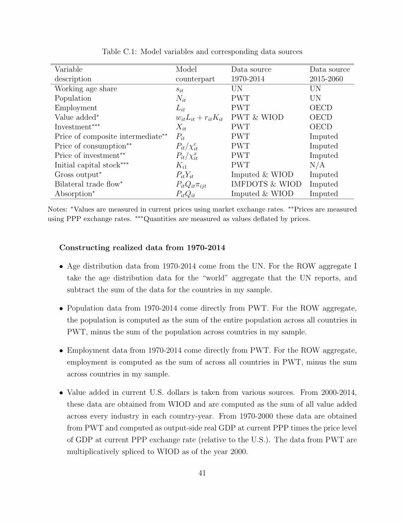
Table C.1: Model variables and corresponding data sources

Variable Model Data source Data sourcedescription counterpart 1970-2014 2015-2060Working age share sit UN UNPopulation Nit PWT UNEmployment Lit PWT OECDValue added∗ witLit + ritKit PWT & WIOD OECDInvestment∗∗∗ Xit PWT OECDPrice of composite intermediate∗∗ Pit PWT ImputedPrice of consumption∗∗ Pit/χ

cit PWT Imputed

Price of investment∗∗ Pit/χxit PWT Imputed

Initial capital stock∗∗∗ Ki1 PWT N/AGross output∗ PitYit Imputed & WIOD ImputedBilateral trade flow∗ PitQitπijt IMFDOTS & WIOD ImputedAbsorption∗ PitQit Imputed & WIOD Imputed

Notes: ∗Values are measured in current prices using market exchange rates. ∗∗Prices are measured

using PPP exchange rates. ∗∗∗Quantities are measured as values deflated by prices.

Constructing realized data from 1970-2014

• Age distribution data from 1970-2014 come from the UN. For the ROW aggregate I

take the age distribution data for the “world” aggregate that the UN reports, and

subtract the sum of the data for the countries in my sample.

• Population data from 1970-2014 come directly from PWT. For the ROW aggregate,

the population is computed as the sum of the entire population across all countries in

PWT, minus the sum of the population across countries in my sample.

• Employment data from 1970-2014 come directly from PWT. For the ROW aggregate,

employment is computed as the sum of across all countries in PWT, minus the sum

across countries in my sample.

• Value added in current U.S. dollars is taken from various sources. From 2000-2014,

these data are obtained from WIOD and are computed as the sum of all value added

across every industry in each country-year. From 1970-2000 these data are obtained

from PWT and computed as output-side real GDP at current PPP times the price level

of GDP at current PPP exchange rate (relative to the U.S.). The data from PWT are

multiplicatively spliced to WIOD as of the year 2000.

41

• Price of consumption from 1970-2014 is computed directly from PWT. For ROW, it is

computed as the ratio of consumption in current prices relative to consumption in PPP

prices. Consumption in ROW is computed as the sum across all countries in PWT

minus the sum across countries in my sample.

• Price of investment is computed analogously to the price of consumption.

• Price of the composite intermediate good from 1970-2014 is constructed using various

data in PWT. I take a weighted average of the price level of imports and of exports,

each of which come directly from PWT. The weight applied to imports is the country’s

import share in total absorption, and the weight applied to exports is the country’s

home trade share in total absorption. Trade and absorption data are described below.

For ROW, I compute the price of imports as the ratio of ROW imports in current

prices divided by ROW imports in PPP prices. ROW imports is computed as the sum

of imports across all countries in PWT minus the sum across countries in my sample.

• Investment quantities from 1970-2014 is computed from various data in the PWT. I be-

gin by computing the nominal investment rate (ratio of expenditures on investment as

a share of GDP in current prices). I then multiply the nominal investment rate by GDP

in current U.S. dollars to arrive at total investment spending in current U.S. dollars.

Finally, I deflate the current investment expenditures by the price of investment.

• Initial capital stock is taken directly from PWT. Capital stock in ROW is computed

as the sum across all countries in PWT minus the sum across countries in my sample.

• Gross output in current U.S. dollars from 2000-2014 is obtained from WIOD and are

computed as the sum of all gross output across every industry in each country-year.

Prior to 2000, I impute these data using the ratio of value added to gross output in

2000, and applying that ratio to scale value added in each year prior to 2000.

• Bilateral trade in current U.S dollars from 2000-2014 is computed directly from WIOD

as the sum of all trade flows (intermediate usage and final usage) across all indus-

tries. Prior to 2000, bilateral trade flows are obtained from the IMFDOTS. Bilateral

trade flows with ROW are computed as imports (exports) to (form ) the world minus

the sum of imports (exports) to (from) the countries in my sample. These data are

multiplicatively spliced to the WIOD data as of the year 2000.

42

• Absorption in current U.S. dollars from 2000-2014 is computed using WIOD data as

gross output minus net exports, summed across all industries.

Constructing projected data from 2015-2060

• Age distribution data from 2015-2060 come from the UN. For the ROW aggregate I

take the age distribution data for the “world” aggregate that the UN reports, and

subtract the sum of the data for the countries in my sample.

• Population data from 2015-2060 are taken directly from UN and spliced to the PWT

levels as of the year 2014.

• Employment data from 2015-2060 are taken directly from OECD and spliced to the

PWT levels as of the year 2014.

• From 2015-2060, data on value added in current U.S. dollars these data are obtained

from OECD projections and computed as real GDP per capita (in constant, local

currency units) times the population times the price level (in local currency units) times

the PPP level (relative to the U.S.) times the nominal exchange rate (local currency

per U.S. dollar at current market prices). The data from OECD are multiplicatively

spliced to WIOD as of the year 2014.

• Price of consumption from 2015-2060 is imputed by assuming equal growth rates to

the price deflator for aggregate GDP, where the price deflator for aggregate GDP is

directly computed using data in the OECD projections.

• Price of investment (P x) from 2015-2060 is imputed using information on its co-

movement with the price of consumption (P c). In particular, I estimate the rela-

tionship between growth in the relative price against a constant and a one-year lag in

the relative price growth, for the years 1972-2014.

ln

(P cit/P

xit

P cit−1/P

xit−1

)= β0 + β1 ln

(P cit−1/P

xit−1

P cit−2/P

xit−2

)+ εit. (C.1)

I use the estimates from equation (C.1) to impute the sequence of prices for investment

from 2015-2060, given the already imputed data for the price of consumption during

these years.

43

• Price of the composite intermediate good from 2015-2060 is imputed by first construct-

ing data for the price of imports of exports. Prices of imports and exports are computed

analogously to the price of investment by estimating equation (C.1) for each series. I

then take a weighted average of the price levels of imports and of exports to determine

the price of the composite good. The weight applied to imports is the country’s import

share in total absorption, and the weight applied to exports is the country’s home trade

share in total absorption. Trade and absorption data are described below.

• Investment quantities from 2015-2060 are computed from various variables in the

OECD projections. I begin by imputing the nominal investment rate (ratio of expen-

ditures on investment to GDP in current prices) using information on its co-movement

with the relative prices. I estimate the relationship between the investment rate against

a country-fixed effect, the lagged investment rate, the contemporaneous and lagged rel-

ative price of investment, and the contemporaneous and lagged real GDP per capita

for the years 1972-2014. Letting ρit = PxitXitGDPit

denote the investment rate,

ln

(ρit

1− ρit

)= αi + β1 ln

(ρit−1

1− ρit−1

)+ β2 ln

(P xit

P cit

)+ β3 ln

(P xit−1

P cit−1

)+ β4 ln(yit) + β5 ln(yit−1) + εit. (C.2)

Using ln (ρ/(1− ρ)) to ensures that the imputed values of ρ are bounded between 0

and 1. I use the estimated coefficients from equation (C.2) together with projections

on the relative price and income per capita to construct projections for the investment

rate. I then multiply the nominal investment rate by GDP in current U.S. dollars

(available in the OECD projections) to arrive at total investment spending in current

U.S. dollars. Finally, I deflate the investment expenditures by the price of investment.

• Gross output in current U.S. dollars from 2015-2060 is imputed using the ratio of value

added to gross output in 2014, and applying that ratio to scale value added in each

year after 2014. The value added data (GDP in current U.S. dollars) after 2014 is

obtained directly from OECD projections.

• Bilateral trade in current U.S dollars from 2015-2060 are constructed in multiple steps.

First, let xijt =Xijt

GOjt−EXPjt be the ratio of country j’s exports to country i, relative

to country j’s gross output net of its total exports. I then estimate how changes

in this trade share co-moves with changes in the importer’s aggregate import price

44

index, changes in the exporter’s aggregate export price index, and changes in both the

importer’s and exporter’s levels of GDP:

ln

(xijtxijt−1

)= β1 ln

(Pmit

Pmit−1

)+ β2 ln

(P xjt

P xjt−1

)+ β3 ln

(GDPitGDPit−1

)+ β4 ln

(GDPjtGDPjt−1

)+ εit. (C.3)

I use the estimated coefficients from equation (C.3) together with projections of prices

of imports and of exports and levels of GDP to construct trade shares from 2015-2060.

In the second step, I use the fact that country i’s domestic sales is determined by

Xiit =GOit

1 +∑

j 6=i xjit,

where gross output and trade shares from 2015-2060 have already been constructed.

Finally, given projected domestic sales and trade shares, the bilateral trade flow is

Xijt = Xjjtxijt.

• Absorption in current U.S. dollars from 2015-2060 is gross output minus net exports.

D Equilibrium conditions

This section describes the solution to a perfect foresight equilibrium.

D.1 Household optimization

The representative household’s optimal path for consumption satisfies two Euler equations:

Cit+1/Nit+1

Cit/Nit

= βσ(ψit+1

ψit

)σ 1 + qt+1

Pit+1/χcit+1

Pit/χcit

σ

, (D.1)

Cit+1/Nit+1

Cit/Nit

= βσ(ψit+1

ψit

)σ rit+1

Pit+1/χcit+1−(χcit+1

χxit+1

)Φ2(Kit+2, Kit+1)(

χcitχxit

)Φ1(Kit+1, Kit)

σ (1− τ kit+1

1− τ kit

)σ.

(D.2)

45

The first Euler equation describes the trade-off between consumption and saving in one-

period bonds, while the second Euler equation describes the trade-off between consumption

and investment in physical capital. Recall that Xit ≡ Φ(Kit+1, Kit) is investment, where Φ1

and Φ2 are the derivatives with respect to the first and second arguments, respectively.

Labor supply in each period is chosen to satisfy

LitNit

= 1− (ζit)φ

(wit

Pit/χcit

)−φ(CitNit

)φ/σ. (D.3)

Given Ki1 and Ai1, the paths of consumption, net-purchases of bonds, investment in

physical capital, and labor supply must satisfy the budget constraint and the accumulation

technologies for capital and net-foreign assets:

PitχcitCit +Ait+1 =

(ritKit −

Pitχxit

Φ(Kit+1, Kit)

)(1− τ kit) + witLit + (1 + qt)Ait + Tit. (D.4)

D.2 Firm optimization

Markets are perfectly competitive so firms set prices equal to marginal costs. Omitting time

subscripts for now, denote the price of variety v, produced in country j and purchased by

country i, as pij(v). Then pij(v) = pjj(v)dij, where pjj(v) is the marginal cost of producing

variety v in country j. Since country i purchases each variety from the country that can

deliver it at the lowest price, the price in country i is pi(v) = minj=1,...,I [pjj(v)dij]. The price

of the composite intermediate good in country i at time t is then

Pit = γ

[I∑j=1

(A−νjtjt ujtdijt

)−θ]− 1θ

, (D.5)

where ujt =(

rjtανjt

)ανjt ( wjt(1−α)νjt

)(1−α)νjt ( Pjt1−νjt

)1−νjtis the unit cost for a bundle of inputs

for intermediate-goods producers in country j at time t.

Next I define total factor usage (K,L,M) and output (Y ) by summing over varieties.

Kit =

∫ 1

0

Kit(v)dv, Lit =

∫ 1

0

Lit(v)dv,

Mit =

∫ 1

0

Mit(v)dv, Yit =

∫ 1

0

Yit(v)dv.

46

The term Lit(v) denotes the quantity of labor employed in the production of variety v at

time t. If country i imports variety v at time t, then Lit(v) = 0. Hence, Lit is the total

quantity of labor employed in country i at time t. Similarly, Kit is the total quantity of

capital used, Mit is the total quantity of the composite good used as an intermediate input

in production, and Yit is the total quantity of output produced.

Cost minimization by firms implies that factor expenses exhaust the value of output.

ritKit = ανitPitYit, witLit = (1− α)νitPitYit, PitMit = (1− νit)PitYit.

That is, ανit is the fraction of the value of production that compensates capital services,

(1 − α)νit is the fraction that compensates labor services, and 1 − νit is the fraction that

covers the cost of intermediate inputs; there are zero profits.

Trade flows The fraction of country i’s expenditures allocated to intermediate varieties

produced by country j is given by

πijt =

(A−νjtjt ujtdijt

)−θ∑I

j=1

(A−νjtjt ujtdijt.

)−θ . (D.6)

D.2.1 Market clearing conditions

Revenues from distortionary capital taxes are returned in lump sum to the household:

τ kitritKit = Tit.

The supply of the composite good, which is an aggregate of all imported and domestic

varieties, must equal the demand., which consists of consumption, investment, and interme-

diate input.Citχcit

+Xit

χxit+Mit = Qit.

Finally, the balance of payments must hold in each country: the current account equals

net exports plus net-foreign income. With net exports equal to gross output less gross

absorption, this condition implies

Bit = PitYit − PitQit + qtAit.

47

D.3 Remark

The world interest rate is strictly nominal. As such, the value plays essentially no role

other than pinning down a numeraire. Since my choice of numeraire is world GDP in each

period, the world interest rate reflects the relative valuation of world GDP at two points

in time. This interpretation is useful in guiding the solution procedure and also makes for

straightforward mapping between model and data. That is, in the model the prices map

into current units, as opposed to constant units. In other words, the model can be rewritten

so that all prices are quoted in time-1 units (like an Arrow-Debreu world) with the world

interest rate of zero and the equilibrium would yield identical quantities.

E Solution algorithm

In this section of the Appendix I describe the algorithm for computing the equilibrium

transition path. Before going further into the algorithm, I introduce some notation. I

denote the cross-country vector of a given variable at a point in time using vector notation,

i.e., ~Kt = {Kit}Ii=1 is the vector of capital stocks across countries at time t.

E.1 Computing the equilibrium transition path

Given the initial conditions— ~K1, ~A1—the equilibrium transition path consists of 15 objects:

{~wt}Tt=1, {~rt}Tt=1, {qt}Tt=1, {~Pt}Tt=1, {~Yt}Tt=1, { ~Qt}Tt=1, {~Ct}Tt=1, { ~Xt}Tt=1, { ~Kt}T+1t=1 , {~Lt}Tt=1,

{ ~Mt}Tt=1, { ~Bt}Tt=1, { ~At}Tt=1, {~Tt}Tt=1, and {~~πt}Tt=1 (I use the double-arrow notation on ~~πt to

indicate that this is an I × I matrix in each period t). Table E.1 provides a list of 15

equilibrium conditions that these objects must satisfy.

The solution procedure is boils down to two loops. The outer loop consists of iterating

on the labor supply decision and the rate of investment in physical capital. The inner loop

consists of iterating on a set of excess demand equations as in Sposi (2012), given the guess

for labor supply and investment rates. First, for the outer loop, guess at the sequence

of labor supply and investment rate for every country in every period. Given the labor

supply and investment rate, within the inner loop start with an initial guess for the entire

sequences of wage vectors and the world interest rate on bonds. Form these two objects,

recover all remaining prices and quantities, across countries and throughout time, using

optimality conditions and market clearing conditions, excluding the balance of payments

condition. Then use departures from the the balance of payments condition to update the

48

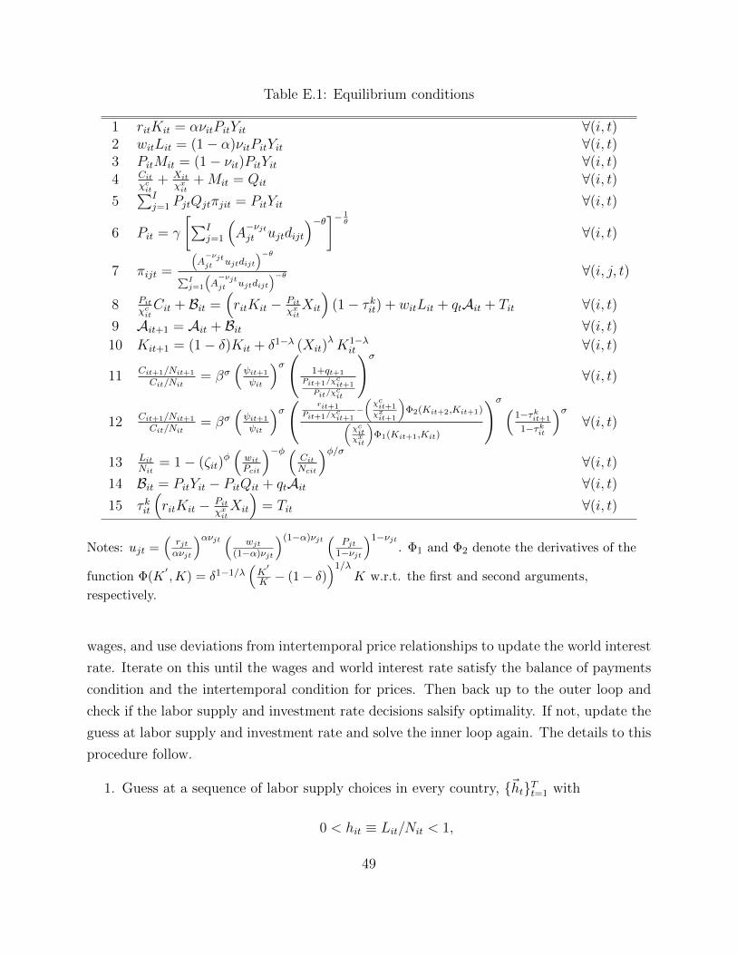
Table E.1: Equilibrium conditions

1 ritKit = ανitPitYit ∀(i, t)2 witLit = (1− α)νitPitYit ∀(i, t)3 PitMit = (1− νit)PitYit ∀(i, t)4 Cit

χcit+ Xit

χxit+Mit = Qit ∀(i, t)

5∑I

j=1 PjtQjtπjit = PitYit ∀(i, t)

6 Pit = γ

[∑Ij=1

(A−νjtjt ujtdijt

)−θ]− 1θ

∀(i, t)

7 πijt =

(A−νjtjt ujtdijt

)−θ∑Ij=1

(A−νjtjt ujtdijt

)−θ ∀(i, j, t)

8 PitχcitCit + Bit =

(ritKit − Pit

χxitXit

)(1− τ kit) + witLit + qtAit + Tit ∀(i, t)

9 Ait+1 = Ait + Bit ∀(i, t)10 Kit+1 = (1− δ)Kit + δ1−λ (Xit)

λK1−λit ∀(i, t)

11 Cit+1/Nit+1

Cit/Nit= βσ

(ψit+1

ψit

)σ(1+qt+1

Pit+1/χcit+1

Pit/χcit

)σ

∀(i, t)

12 Cit+1/Nit+1

Cit/Nit= βσ

(ψit+1

ψit

)σ( rit+1Pit+1/χ

cit+1−(χcit+1χxit+1

)Φ2(Kit+2,Kit+1)(

χcitχxit

)Φ1(Kit+1,Kit)

)σ (1−τkit+1

1−τkit

)σ∀(i, t)

13 LitNit

= 1− (ζit)φ(witPcit

)−φ (CitNcit

)φ/σ∀(i, t)

14 Bit = PitYit − PitQit + qtAit ∀(i, t)15 τ kit

(ritKit − Pit

χxitXit

)= Tit ∀(i, t)

Notes: ujt =(rjtανjt

)ανjt ( wjt(1−α)νjt

)(1−α)νjt ( Pjt1−νjt

)1−νjt. Φ1 and Φ2 denote the derivatives of the

function Φ(K′,K) = δ1−1/λ

(K′

K − (1− δ))1/λ

K w.r.t. the first and second arguments,

respectively.

wages, and use deviations from intertemporal price relationships to update the world interest

rate. Iterate on this until the wages and world interest rate satisfy the balance of payments

condition and the intertemporal condition for prices. Then back up to the outer loop and

check if the labor supply and investment rate decisions salsify optimality. If not, update the

guess at labor supply and investment rate and solve the inner loop again. The details to this

procedure follow.

1. Guess at a sequence of labor supply choices in every country, {~ht}Tt=1 with

0 < hit ≡ Lit/Nit < 1,

49

guess a sequence of nominal investment rates, {~ρt}Tt=1 with

0 < ρit ≡(Pit/χ

xit)Xit

witLit/(1− α)< 1,

and guess at a terminal NFA position in each country, AiT+1, with∑I

i=1AiT+1 = 0.

Take these as given for the next sequence of steps.

(a) Guess the entire path for wages, {~wt}Tt=1, across countries and the entire path for

the world interest rate, {qt}Tt=2, such that∑

iwitLit1−α = 1 (∀t).

(b) In period 1 set ~r1 =(

α1−α

) (~w1~H1~K1

), where the initial stock of capital is prede-

termined. Compute prices ~P1 using condition 6 in Table E.1. Solve for physical

investment, ~X1, using the guess for the nominal investment rate together with

prices: ~X1 = ~ρ1 ~w1~L1

(1−α)(~P1/~χx1 )and for the next-period capital stock, ~K2, using condi-

tion 10. Repeat this set of calculations for period 2, then for period 3, and all the

way through period T .

(c) Compute the bilateral trade shares {~~πt}Tt=1 using condition 7.

(d) This step is slightly more involved. I show how to compute the path for consump-

tion and bond purchases by solving the intertemporal problem of the household.

This is done in three parts. First I derive the lifetime budget constraint, second

I derive the fraction of lifetime wealth allocated to consumption at each period t,

and third I recover the sequences for bond purchases and the stock of NFAs.

Deriving the lifetime budget constraint To begin, compute the lifetime

budget constraint for the representative household (omitting country subscripts

for now). Begin with the period budget constraint from condition 8 and combine

it with the NFA accumulation technology in condition 9 and the balanced tax

revenue in condition 15:

At+1 = rtKt + wtLt −PtχcCt −

PtχxtXt + (1 + qt)At.

Iterate the period budget constraint forward through time and derive a lifetime

budget constraint. Given Ai1 > 0, compute the NFA position at time t = 2:

A2 = r1K1 + w1L1 −P1

χc1C1 −

P1

χx1X1 + (1 + q1)A1.

50

Similarly, compute the NFA position at time t = 3:

A3 = r2K2 + w2L2 −P2

χc2C2 −

P2

χx2X2 + (1 + q2)A2

⇒ A3 = r2K2 + w2L2 −P2

χx2X2 + (1 + q2)

(r1K1 + w1L1 −

P1

χx1X1

)− P2

χc2C2 − (1 + q2)

P1

χc1C1 + (1 + q2)(1 + q1)Ai1.

Continue to period 4 in a similar way

A4 = r3K3 + w3L3 − P3C3 −P3

χx3X3 + (1 + q3)A3

⇒ A4 = r3K3 + w3L3 −P3

χx3X3

+ (1 + q3)

(r2K2 + w2L2 −

P2

χx2X2

)+ (1 + q3)(1 + q2)

(r1K1 + w1L1 −

P1

χx1X1

)− P3

χc3C3 − (1 + q3)

P2

χc2C2 − (1 + q3)(1 + q2)

P1

χc1C1 + (1 + q3)(1 + q2)(1 + q1)A1.

Before proceeding, it is useful to define (1 +Qt) =∏t

n=1 (1 + qn).

⇒ A4 =(1 +Q3)

(r3K3 + w3L3 − P3

χx3X3

)(1 +Q3)

+(1 +Q3)

(r2K2 + w2L2 − P2

χx2X2

)(1 +Q2)

+(1 +Q3)

(r1K1 + w1L1 − P1

χx1X1

)(1 +Q1)

−(1 +Q3)P3

χc3C3

(1 +Q3)−

(1 +Q3)P2

χc2C2

(1 +Q2)−

(1 +Q3)P1

χc1C1

(1 +Q1)+ (1 +Q3)A1.

By induction, for any time t,

At+1 =t∑

n=1

(1 +Qt)(rnKn + wnLn − Pn

χxnXn

)(1 +Qn)

−t∑

n=1

(1 +Qt)PnχcnCn(1 +Qn)

+ (1 +Qt)A1

⇒ At+1 = (1 +Qt)

(t∑

n=1

rnKn + wnLn − PnχxnXn

(1 +Qn)−

t∑n=1

PnχcnCn

(1 +Qn)+A1

).

51

Observe the previous expression as of t = T to derive the lifetime budget con-

straint:

T∑n=1

PnχcnCn

(1 +Qn)=

T∑n=1

rnKn + wnLn − PnχxnXn

(1 +Qn)+A1 −

AT+1

(1 +QT )︸ ︷︷ ︸W

. (E.1)

In the lifetime budget constraint (E.1), W denotes the net present value of lifetime

wealth, taking both the initial and terminal NFA positions as given.

Solving for the path of consumption Next, compute how the net-present

value of lifetime wealth is optimally allocated throughout time. The Euler equa-

tion for bonds (condition 11) implies the following relationship between consump-

tion in any two periods t and n:

Cn =

(Nn

Nt

)βσ(n−t)

(ψnψt

)σ (1 +Qn1 +Qt

)σ (Pt/χ

ct

Pn/χcn

)σCt

⇒PnχcnCn

1 +Qn=

(Nn

Nt

)βσ(n−t)

(ψnψt

)σ (1 +Qn1 +Qt

)σ−1(Pt/χ

ct

Pn/χcn

)σ−1 PtχctCt

1 +Qt.

Since equation (E.1) implies that∑T

n=1

PinχcinCin

1+Qn = W , rearrange the previous ex-

pression (putting country subscripts back in) to obtain

PitχcitCit

1 +Qit=

Nitβσtψσit(1 +Qit)σ−1

(Pitχcit

)1−σ

∑Tn=1Ninβσnψσin(1 +Qin)σ−1

(Pinχcin

)1−σ

︸ ︷︷ ︸

ξit

Wi. (E.2)

That is, in period t the household in country i spends a share ξit of lifetime wealth

on consumption, with∑T

t=1 ξit = 1 for all i. Note that ξit depends only on prices.

Computing bond purchases and the NFA positions In period 1 take as

given consumption spending, investment spending, capital income, labor income,

and net income from the initial NFA position; each of which have already been

computed in previous steps. Then solve for net bond purchases { ~Bt}Tt=1 using

the period budget constraint in condition 8. Use condition 9 to solve for the

52

NFA position in period 2. Repeat this set of calculations iteratively for periods

2, . . . , T .

Trade balance condition I compute an excess demand equation as in Alvarez

and Lucas (2007), but instead of imposing that net exports equal zero in each

country, I impose that net exports equal the current account less net foreign

income from assets.

Zwit

({~wt, qt}Tt=1

)=PitYit − PitQit −Bit + qtAit

wit.

Condition 14 requires that Zwit

({~wt, qt}Tt=1

)= 0 for all (i, t). If this is different

from zero in at least some country at some point in time update the wages as

follows.

Λwit

({~wt, qt}Tt=1

)= wit

(1 + κ

Zwit

({~wt, qt}Tt=1

)Lit

)is the updated wages, where κ is chosen to be sufficiently small so that Λw > 0.

Normalizing model units The last part of this step is updating the equilib-

rium world interest rate. Recall that the numeraire is defined to be world GDP

at each point in time:∑I

i=1(ritKit + witLit) = 1 (∀t). For an arbitrary sequence

of {qt+1}Tt=1, this condition need not hold. As such, update the the world interest

rate as

1 + qt =

∑Ii=1(rit−1Kit−1 + Λw

it−1Lit−1)∑Ii=1(ritKit + Λw

itLit)for t = 2, . . . , T. (E.3)

The values for capital stock and the rental rate of capital are computed in step 2,

while the values for wages are the updated values Λw above. I set q1 = 1−ββ

(the

interest rate that prevails in a steady state) and chose Ai1 so that q1Ai1 matches

the desired initial NFA position in current prices.

Having updated the wages and the world interest rate, return to step 2a and

perform each step again. Iterate through this procedure until the excess demand is

sufficiently close to zero. In the computations I find that my preferred convergence

metric:T

maxt=1

{I

maxi=1

{|Zw

it

({~wt, qt}Tt=1

)|}}

converges roughly monotonically towards zero.

53

2. The last step of the algorithm is to update the labor supply, investment rate, and

terminal NFA position. Until now, the optimality condition 13 for the labor supply

and condition 12 for the investment in physical capital have not been used. As such,

compute a “residual” as to each of these first-order conditions as

Zhit

({~hit}Tt=1

)= 1− ζφit

(witPcit

)−φ(CitNcit

)φ/σ−(LitNit

),

Zρit

({~ρit}Tt=1

)= βσ

(ψit+1

ψit

)σ rit+1

Pit+1/χcit+1−(χcit+1

χxit+1

)Φ2(Kit+2, Kit+1)(

χcitχxit

)Φ1(Kit+1, Kit)

σ (1− τ kit+1

1− τ kit

)σ

−(Cit+1/Nit+1

Cit/Nit

).

Condition 13 requires that Zhit

({~hit}Tt=1

)= 0 for all (i, t), while condition 11 requires

that Zρit

({~ρit}Tt=1

)= 0. Update the labor supply and investment rate as

Λhit

({~ht}Tt=1

)= hit

(1 + ψZh

it

({~ht}Tt=1

)),

Λρit

({~ρt}Tt=1

)= ρit

(1 + ψZh

it

({~ρt}Tt=1

)),

where ψ is a constant value assigned to ensure that the updated guesses remain positive.

Given the updated sequence of labor supply and investment rate, return to step 1.

With T chosen to be sufficiently large, the turnpike theorem implies that the terminal

NFA position has no bearing on the transition path up to some time t? < T (see Maliar,

Maliar, Taylor, and Tsener, 2015).

F Robustness

This section of the Appendix considers alternative specifications for decomposing wedges

into demographic and distortionary components.

F.1 High- and low-variant demographic projections

Projections for the age distribution involve uncertainty surrounding fertility, migration flows,

and death rates. The UN provides different variants of the projections, each of which yield

different projected paths for each country’s population and each country’s age distribution

54

of the population. The main part of the paper used the medium-variant projections. Two

other readily available projections are the high-variant and low-variant projections.

According to the UN, “A medium (or standard) variant is the most likely demographic

development (forecast?). High and low variants are considered the reasonable upper and

lower limits of realistic projections and indicate the margin of uncertainty.”

For each variant of the projections, I repeat the entire quantitative exercise as follows.

First, taking the relevant variant for projected population population levels, I implement the

wedge accounting procedure and calibrate all country-specific and time-varying parameters of

the model. Second, taking the relevant variant for projected age distributions, I decompose

the wedges into demographic and distortionary components using OLS, exactly as in the

paper. Finally, I consider a counterfactual in which each country’s working age share is

unilaterally held fixed at its 1970 levels. I prefer to compare the unilateral counterfactuals

since the high and low bounds of the projections differ across countries.

The elasticity between the ratio of net exports to GDP and labor productivity growth,

using the counterfactual data from 1970-2014, is similar across all variants of the projections.

In the low-variant counterfactual, the elasticity is -0.77 and in the high-variant counterfactual

the elasticity is -1.03. Recall that the elasticity is the medium-variant counterfactual is -0.94.

F.2 Alternative empirical specifications for wedge decomposition

In the main paper, decomposition of the wedges assumed that the log-wedge is linear in

the working age share. This was specified intentionally to impose a conservative mapping

between demographics and wedges. In this robustness exercise I specify that the log-wedge

is a polynomial of order H = 3 in the working age share.

ln

(Nit

Nit−1

)= γNi + κNt−1 +

H∑h=1

µNh × shit−1 + εNit−1; i = 1, . . . I; t = 2, . . . T,

ln

(ψitψit−1

)= γψi +

H∑h=1

µψh × (sit−1 − sUt−1)h + εψit−1; i = 1, . . . I (ex. U.S.); t = 2, . . . T,

ln (ζit) = γζi + κζt +H∑h=1

µζh × shit + εζit; i = 1, . . . I; t = 1, . . . T.

I decompose the wedges using this specification and compute the counterfactual in which

every country’s age share vectors are held fixed at their 1970 levels. In the counterfactual,

55

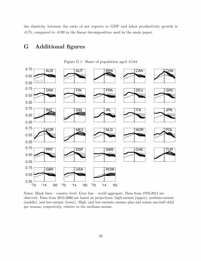
the elasticity between the ratio of net exports to GDP and labor productivity growth is

-0.75, compared to -0.90 in the linear decomposition used in the main paper.

G Additional figures

Figure G.1: Share of population aged 15-64

0.35

0.55

0.75AUS

WLD

AUT BRA CAN CHN

0.35

0.55

0.75DNK FIN FRA DEU GRC

0.35

0.55

0.75IND IDN IRL ITA JPN

0.35

0.55

0.75KOR MEX NLD NOR POL

0.35

0.55

0.75PRT ESP SWE CHE TUR

'70 '14 '60

0.35

0.55

0.75GBR

'70 '14 '60

USA

'70 '14 '60

ROW

Notes: Black lines – country level. Gray line – world aggregate. Data from 1970-2014 areobserved. Data from 2015-2060 are based on projections: high-variant (upper), medium-variant(middle), and low-variant (lower). High- and low-variants assume plus and minus one-half childper woman, respectively, relative to the medium-variant.

56

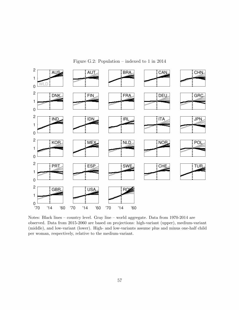
Figure G.2: Population – indexed to 1 in 2014

0

1

2AUS

WLD

AUT BRA CAN CHN

0

1

2DNK FIN FRA DEU GRC

0

1

2IND IDN IRL ITA JPN

0

1

2KOR MEX NLD NOR POL

0

1

2PRT ESP SWE CHE TUR

'70 '14 '60

0

1

2GBR

'70 '14 '60

USA

'70 '14 '60

ROW

Notes: Black lines – country level. Gray line – world aggregate. Data from 1970-2014 areobserved. Data from 2015-2060 are based on projections: high-variant (upper), medium-variant(middle), and low-variant (lower). High- and low-variants assume plus and minus one-half childper woman, respectively, relative to the medium-variant.

57

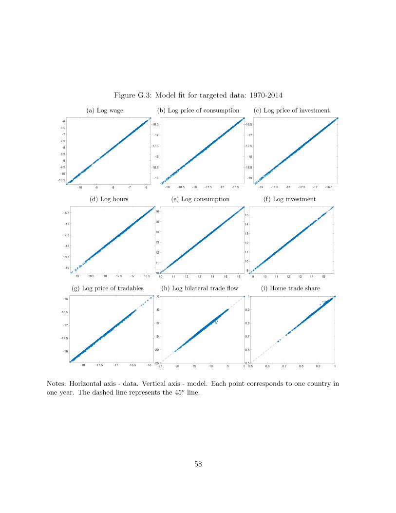
Figure G.3: Model fit for targeted data: 1970-2014

(a) Log wage

-10 -9 -8 -7 -6

-10.5

-10

-9.5

-9

-8.5

-8

-7.5

-7

-6.5

-6

(b) Log price of consumption

-19 -18.5 -18 -17.5 -17 -16.5

-19

-18.5

-18

-17.5

-17

-16.5

(c) Log price of investment

-19 -18.5 -18 -17.5 -17 -16.5

-19

-18.5

-18

-17.5

-17

-16.5

(d) Log hours

-19 -18.5 -18 -17.5 -17 -16.5

-19

-18.5

-18

-17.5

-17

-16.5

(e) Log consumption

10 11 12 13 14 15 16

10

11

12

13

14

15

16

(f) Log investment

9 10 11 12 13 14 15

9

10

11

12

13

14

15

(g) Log price of tradables

-18 -17.5 -17 -16.5 -16

-18

-17.5

-17

-16.5

-16

(h) Log bilateral trade flow

-25 -20 -15 -10 -5 0-25

-20

-15

-10

-5

0

(i) Home trade share

0.5 0.6 0.7 0.8 0.9 10.5

0.6

0.7

0.8

0.9

1

Notes: Horizontal axis - data. Vertical axis - model. Each point corresponds to one country inone year. The dashed line represents the 45o line.

58

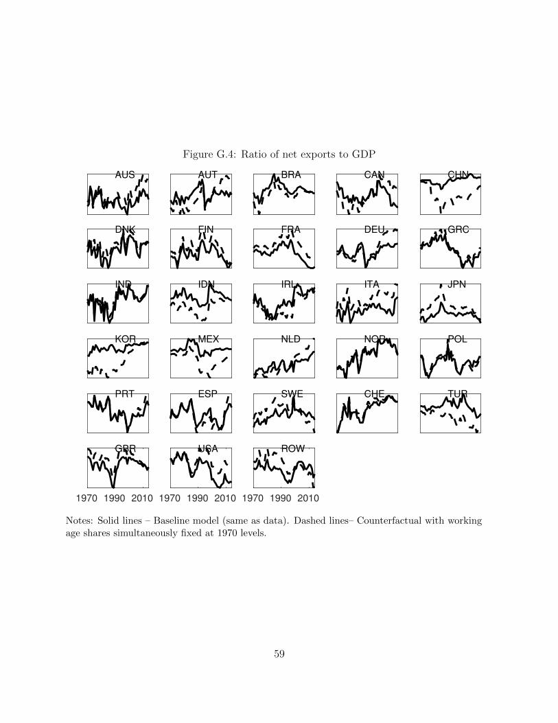
Figure G.4: Ratio of net exports to GDP

AUS AUT BRA CAN CHN

DNK FIN FRA DEU GRC

IND IDN IRL ITA JPN

KOR MEX NLD NOR POL

PRT ESP SWE CHE TUR

1970 1990 2010

GBR

1970 1990 2010

USA

1970 1990 2010

ROW

Notes: Solid lines – Baseline model (same as data). Dashed lines– Counterfactual with workingage shares simultaneously fixed at 1970 levels.

59