Embed Size (px)
Citation preview

Demographics and Real Interest Rates:Inspecting the Mechanism∗
Carlos Carvalho
PUC-Rio
Andrea Ferrero
University of Oxford
Fernanda Nechio
FRB San Francisco
September 28, 2015
Abstract
The demographic transition can affect the equilibrium real interest rate through three channels.
An increase in longevity—or expectations thereof—puts downward pressure on the real interest
rate, as agents build up their savings in anticipation of a longer retirement period. A reduction
in the population growth rate has two counteracting effects. On the one hand, capital per-worker
rises, thus inducing lower real interest rates through a reduction in the marginal product of capital.
On the other hand, the decline in population growth eventually leads to a higher dependency ratio
(the fraction of retirees to workers). Because retirees save less than workers, this compositional
effect lowers the aggregate savings rate and pushes real rates up. We calibrate a tractable life-cycle
model to capture salient features of the demographic transition in developed economies, and find
that its overall effect is to lower the equilibrium interest rate by one and a half percentage points
between 1990 and 2014. Through these channels, demographic trends have important implications
for the conduct of monetary policy, especially in light of the zero lower bound on nominal interest
rates. Other policies can offset the negative effects of the demographic transition on real rates with
different degrees of success.
JEL codes: E52, E58, J11
Keywords: Life expectancy, population growth, demographic transition, real interest rate,
monetary policy
∗This paper was prepared for the 2015 Conference on “Post-Crisis Slump,” to be held at the European Commission
in Brussels on October 1-2, 2015. For comments and suggestions, we thank seminar participants at the Bundesbank
and Nova School of Business. The views expressed in this paper do not necessarily reflect the position of the Federal
Reserve Bank of San Francisco or of the Federal Reserve System. Eric Hsu provided excellent research assistance. Emails:
[email protected], [email protected], [email protected].
1

1990 1995 2000 2005 2010
perc
enta
ge p
oint
s
-4
-2
0
2
4
6
8
10Real Short-Term Yields
Median Mean
Figure 1: Ex-post real short-term interest rates, calculated as yields on short-termgovernment securities with maturity less than one year minus realized CPI inflation.The sample consists of Belgium, Germany, Denmark, Finland, France, Greece, Ice-land, Ireland, Italy, Japan, Netherlands, Norway, Portugal, Spain, Sweden, UnitedKingdom, United States. The dashed lines indicate the 90-10 range across countries.
1 Introduction
Since the Global Financial Crisis (GFC), real interest rates in many developed economies have been in
negative territory, as nominal interest rates hover around zero and inflation rates, although quite low for
historical standards, have remained positive (in most countries, at least on average). This observation
naturally brings forth the implication that accommodative monetary policies (both conventional and
unconventional) that were put in place in response to the GFC are the reason behind ultra-low real
rates, and that this phenomenon will be over as soon as central banks will begin the tightening cycle.
Yet, a longer-term perspective immediately reveals a different perspective. Real interest rates have
been trending down for more than two decades across many countries (Figure 1). These low-frequency
movements suggest that forces other than accommodative monetary policies must be at play.
Demographic trends are a natural candidate explanation for low and declining real interest rates.
The world is undergoing a dramatic demographic transition. In most advanced economies people tend
to live longer. In Japan, the U.S. and Western Europe, life expectancy at birth has increased by about
10 years between 1960 and 2010 (Figure 2, left panel), and new generations have continued to expect
longevity to increase. At the same time, immigration notwithstanding, population growth rates are
decreasing at a fast pace, and in some cases (e.g. Japan) becoming negative (Figure 2, right panel).
2

1950 1970 1990 2010 2030 2050 2070 2090
years
60
65
70
75
80
85
90
95
100Life Expectancy
Developed EconomiesJapanUnited StatesWestern Europe
1950 1970 1990 2010 2030 2050 2070 2090
perc
enta
ge p
oin
ts
-1
-0.5
0
0.5
1
1.5
2Population Growth Rate
Developed EconomiesJapanUnited StatesWestern Europe
Figure 2: Left panel: Years of life expectancy at birth. Right panel: Populationgrowth rate. Sample: Developed Economies (Northern America, Europe, Japan,Australia, New Zealand), Japan, United States, Western Europe. Source: UnitedNations World Population Prospects (2015 Revision).
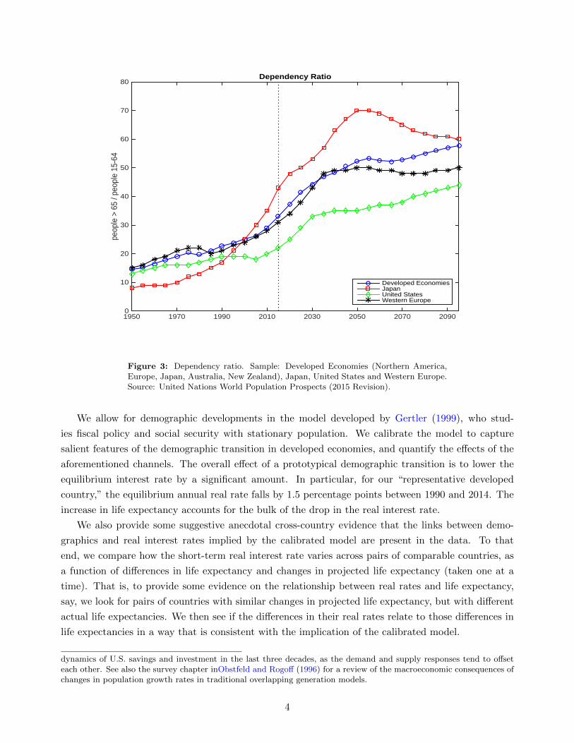
The combination of the population growth slowdown and the increase in longevity implies a notable
increase in the dependency ratio—i.e. the ratio between people 65 years and older and people 15 to
64 years old (Figure 3). The consequences of this demographic transition are far reaching and have
important macroeconomic, public finance and political economic repercussions.1
In this paper, we focus on the consequences of the demographic transition for real interest rates.
We illustrate three channels through which the demographic transition can affect the equilibrium
real interest rate using a tractable life-cycle model. For a given retirement age, an increase in life
expectancy lengthens the retirement period and generates additional incentives to save throughout
the life cycle.2 This effect tends to be stronger if agents believe that public pension systems will not
be able to bear the additional burden generated by an aging population. Therefore, an increase in
longevity—and expectations thereof—tends to put downward pressure on the real interest rate, as
agents build up their savings in anticipation of a longer retirement period.
A drop in the growth rate of the population produces two opposite effects on real interest rates.
On the one hand, lower population growth leads to a higher capital-labor ratio, which depresses the
marginal product of capital. This “supply effect” is very much akin to a permanent slowdown in
productivity growth, pushing down real interest rates. On the other hand, however, lower population
growth eventually drives up the dependency ratio. Because retirees have a lower marginal propensity
to save, this change in the composition of the population is akin to a “demand effect” that pushes up
aggregate consumption, and puts upward pressure on equilibrium real interest rates.3
1See Nishimura (2011) for an excellent discussion of the connections between the demographic transition and therecent global financial crisis.
2Acemoglu and Johnson (2007) study the effects of increases in life expectancy on economic growth. Ferrero (2010)focuses the implication of differentials in life expectancy among advanced economies for international capital flows.
3Chen et al. (2009) and Ferrero (2010) find small effects of measured changes in population growth rates on the
3
1950 1970 1990 2010 2030 2050 2070 2090
peop
le >
65
/ peo
ple
15-6
4
0
10
20
30
40
50
60
70
80Dependency Ratio
Developed EconomiesJapanUnited StatesWestern Europe
Figure 3: Dependency ratio. Sample: Developed Economies (Northern America,Europe, Japan, Australia, New Zealand), Japan, United States and Western Europe.Source: United Nations World Population Prospects (2015 Revision).
We allow for demographic developments in the model developed by Gertler (1999), who stud-
ies fiscal policy and social security with stationary population. We calibrate the model to capture
salient features of the demographic transition in developed economies, and quantify the effects of the
aforementioned channels. The overall effect of a prototypical demographic transition is to lower the
equilibrium interest rate by a significant amount. In particular, for our “representative developed
country,” the equilibrium annual real rate falls by 1.5 percentage points between 1990 and 2014. The
increase in life expectancy accounts for the bulk of the drop in the real interest rate.
We also provide some suggestive anecdotal cross-country evidence that the links between demo-
graphics and real interest rates implied by the calibrated model are present in the data. To that
end, we compare how the short-term real interest rate varies across pairs of comparable countries, as
a function of differences in life expectancy and changes in projected life expectancy (taken one at a
time). That is, to provide some evidence on the relationship between real rates and life expectancy,
say, we look for pairs of countries with similar changes in projected life expectancy, but with different
actual life expectancies. We then see if the differences in their real rates relate to those differences in
life expectancies in a way that is consistent with the implication of the calibrated model.
dynamics of U.S. savings and investment in the last three decades, as the demand and supply responses tend to offseteach other. See also the survey chapter inObstfeld and Rogoff (1996) for a review of the macroeconomic consequences ofchanges in population growth rates in traditional overlapping generation models.
4

Through their effect on the real interest rate, demographic trends can thus be one of the key drivers
of the so-called “Secular Stagnation” hypothesis (Hansen, 1939). In resuscitating this idea, Summers
(2014) has emphasized exactly how in such an environment the equilibrium real interest rate would be
low, and potentially negative. Low and declining real interest rates carry important implications for
the conduct of monetary policy, especially in light of the zero lower bound on monetary policy. The
paper briefly revisits this issue in the context of our framework.
In addition to the diagnostics, the literature on Secular Stagnation puts forth policy suggestions
to ameliorate the problems it highlights. Our analysis formalizes some of these ideas, and allows us to
quantify the effects of specific measures that, at least in principle, can undo or mitigate the effects of
the demographic transition on real rates, such as expansionary fiscal policies and structural reforms.
The rest of the paper proceeds as follows. Section 2 presents the model, with particular focus
on the life-cycle dimension. Section 3 provides some anecdotal evidence on possible links between
demographics and real interest rates, and presents our quantitative experiments based on the calibrated
model. Section 4 studies policies that may mitigate or undo the effects of the demographic transition
on real interest rates. Finally, Section 5 concludes.
2 The Model
The economy consist of three types of economic agents: households, firms, and the government. Indi-
viduals are born workers, and supply inelastically one unit of labor while employed. After retirement,
households consume out of their asset income. The two available saving vehicles are physical capital
and government bonds. Perfectly competitive firms produce a single good (the numeraire) that is used
for both consumption and investment. The government takes spending as given and decides on the
mix of lump-sum taxes and one-period debt to satisfy its budget constraint.
We abstract from aggregate uncertainty and consider the effects of unexpected one-time changes in
demographic parameters in an otherwise perfect-foresight environment. The only source of uncertainty
that may potentially affect agents’ behavior stems from idiosyncratic retirement and death risk. To
keep the model tractable, we make a few assumptions that simplify aggregation without sacrificing
the life-cycle dimension.
2.1 Households and Life-Cycle Structure
At any given point in time, individuals belong to one of two groups: workers (w) or retirees (r). At
time t−1, workers have mass Nwt−1 and retirees have mass N r
t−1. Between periods t−1 and t, a worker
remains in the labor force with probability ωt, and retires otherwise. If retired, an individual survives
from period t − 1 to period t with probability γt.4 In period t, (1− ωt + nt)N
wt−1 new workers are
born. Consequently, the law of motion for the aggregate labor force is
Nwt = (1− ωt + nt)N
wt−1 + ωtN
wt−1 = (1 + nt)N
wt−1, (1)
4Because retirement is an absorbing state in this model, the probability of retiring is perhaps best interpreted as therisk of becoming unable to supply labor.
5

so that nt represents the growth rate of the labor force between periods t − 1 and t. The number of
retirees evolves over time according to
N rt = (1− ωt)Nw
t−1 + γtNrt−1. (2)
From (1) and (2), we define the dependency ratio (ψt ≡ N rt /N
wt ), which summarizes the relevant
heterogeneity in the population and evolves according to
(1 + nt)ψt = (1− ωt) + γtψt−1. (3)
Workers inelastically supply one unit of labor, while retirees do not work.5 Preferences for an
individual of group z = w, r are a restricted version of the recursive non-expected utility family
(Kreps and Porteus, 1978; Epstein and Zin, 1989) that assumes risk neutrality
V zt =
(Czt )ρ + βzt+1 [Et (Vt+1 | z)]ρ
1ρ , (4)
where Czt denotes consumption and V zt stands for the value of utility in period t. Retirees and workers
have different discount factors to account for the probability of death
βzt+1 =
βγt+1 if z = r
β if z = w
The expected continuation value in (4) differs across workers and retirees because of the different
possibilities to transition between groups
Et Vt+1 | z =
V rt+1 if z = r
ωt+1Vwt+1 + (1− ωt+1)V r
t+1 if z = w
This life-cycle model is analytically tractable because the transition probabilities ω and γ are
independent of age and of the time since retirement. With standard risk-averse preferences, however,
this assumption would imply a strong precautionary saving motive for young agents, which is hard to
reconcile with actual consumption/savings choices. Risk-neutral preferences with respect to income
fluctuations prevent a counterfactual excess of savings by young workers (Farmer, 1990; Gertler, 1999).
Nevertheless, the separation of the coefficient of intertemporal substitution (σ ≡ (1− ρ)−1) from risk
aversion implied by (4) allows for a reasonable response of consumption and savings to changes in
interest rates.
Households consume the final good Ct and allocate their wealth among investment in new physical
capital Kt and bonds issued by the government Bt. Households rent the capital stock to firms at a
5Gertler (1999) shows how to introduce variable labor supply in this framework without sacrificing its analyticaltractability. The demographic trends documented in Section 1 should induce individuals to supply more hours andincrease participation rates. The data for all advanced economies, instead, display the opposite tendency, that is, a moreor less pronounced downward trend for both variables. We thus view the assumption of inelastic labor supply as a naturalbenchmark for the purposes of our paper. At the same time, government policies around the world are attempting tofight this course, delaying the retirement age. We return to this issue toward the end of the paper.
6

real rate RKt and bear the cost of depreciation δ ∈ (0, 1). Government bonds Bt pay a gross return
Rt.
2.1.1 Retirees
An individual born in period j and retired in period τ chooses consumption Crt (j, τ) and assets
Krt (j, τ), Br
t (j, τ), for t ≥ τ to solve
V rt (j, τ) = max
(Crt (j, τ))ρ + βγt+1
[V rt+1 (j, τ)
]ρ 1ρ , (5)
subject to
Crt (j, τ) +Krt (j, τ) +Br
t (j, τ) =1
γt
[RKt + (1− δ)]Kr
t−1(j, τ) +Rt−1Brt−1(j, τ)
. (6)
Additionally, the optimization problem is also subject to the consistency requirement that the retiree’s
initial asset holdings upon retirement correspond to the assets held in the last period as a worker, that
is,
Krτ−1 (j, τ) = Kw
τ−1 (j) ,
Brτ−1(j, τ) = Bw
τ−1(j). (7)
At the beginning of each period, retirees turn their wealth over to a perfectly competitive mutual
fund industry which invests the proceeds and pays back a premium over the market return equal to
1/γt, to compensate for the probability of death (Blanchard, 1985; Yaari, 1965). A retiree who survives
between periods t− 1 and t then makes investment decisions right at the end of period t− 1.
Appendix A.1 derives the Euler equations for government bonds and capital that characterize the
problem of a retiree. In the absence of aggregate uncertainty, returns on both assets are equalized
Rt = RKt+1 + (1− δ). (8)
Hence, for convenience, we define total assets for a retiree as
Art (j, τ) ≡ Krt (j, τ) +Br
t (j, τ). (9)
Due to the equality of returns, a retiree’s budget constraint (6) can be rewritten compactly as
Crt (j, τ) +Art (j, τ) =Rt−1A
rt−1(j, τ)
γt. (10)
In Appendix A.1 we show that consumption is a fraction of total wealth
Crt (j, τ) = ξrt
(Rt−1A
rt−1(j, τ)
γt
), (11)
where the marginal propensity to consume satisfies the following first-order non-linear difference equa-
7

tion:1
ξrt= 1 + γt+1β
σ (Rt)σ−1 1
ξrt+1
. (12)
From (11) and (10), asset holdings evolve according to
Art (j, τ) = (1− ξrt )Rt−1A
rt−1(j, τ)
γt.
Finally, the Appendix also shows that the value function for a retiree is linear in consumption
V rt (j, τ) = (ξrt )
σ1−σCrt (j, τ) . (13)
2.1.2 Workers
Workers start their life with zero assets. We write the optimization problem for a worker born in
period j in terms of total assets Awt (j) ≡ Kwt (j) +Bw
t (j). Specifically, a worker chooses consumption
Cwt (j) and assets Awt (j) for t ≥ j to solve
V wt (j) = max
(Cwt (j))ρ + β
[ωt+1V
wt+1 (j) + (1− ωt+1)V r
t+1 (j, t+ 1)]ρ 1
ρ , (14)
subject to
Cwt (j) +Awt (j) = Rt−1Awt−1 (j) +Wt − Twt (15)
and Awj (j) = 0, where Wt represents the real wage and Twt is the total amount of lump-sum taxes
paid by each worker. Workers do not turn their wealth over to the mutual fund industry, and hence do
not receive the additional return that compensates for the probability of death.6 The value function
V rt+1 (j, t+ 1) is the solution of the problem (5) − (10) above and enters the continuation value of
workers, who have to take into account the possibility that retirement occurs between periods t and
t+ 1.
In Appendix A.2 we present the complete solution to a worker’s optimization problem and show
that workers’ consumption is a fraction of total wealth, defined as the sum of financial and non-financial
(“human”) wealth
Cwt (j) = ξwt(Rt−1A
wt−1 (j) +Hw
t
), (16)
where Hwt represents the present discounted value of current and future real wages net of taxation,
and is independent of individual-specific characteristics
Hwt ≡
∞∑v=0
(Wt+v − Twt+v)v∏s=1
Ωt+sRt+s−1
ωt+s
= Wt − Twt +ωt+1H
wt+1
Ωt+1Rt. (17)
As for retirees, workers’ marginal propensity to consume ξwt also evolves according to a first-order
6Allowing workers access to the mutual fund industry would provide complete insurance against the probability ofretirement, hence shutting down most of the interesting life-cycle dimensions of the model.
8
non-linear difference equation:1
ξwt= 1 + βσ (Ωt+1Rt)
σ−1 1
ξwt+1
. (18)
The adjustment term Ωt that appears in (17) and (18) depends on the ratio of the marginal propensity
to consume of retirees and workers
Ωt ≡ ωt + (1− ωt)(ξrtξwt
) 11−σ
.
In the definition of non-financial wealth (17), the term Ωt+1Rtωt+1
constitutes the real effective discount
rate for a worker. The first component of the (higher) discounting captures the effect of the finite
lifetime horizon (less value attached to the future). The term ωt+1 augments the actual discount
factor because workers need to finance consumption during the retirement period (positive probability
of retiring).
The dynamics of asset holdings can then be obtained from the budget constraint of a worker and
the consumption function (16)
Awt (j) +ωt+1H
wt+1
Ωt+1Rt= (1− ξwt )
(Rt−1A
wt−1 (j) +Hw
t
).
Finally, as for retirees, workers’ value function is also linear in their consumption
V wt (j) = (ξwt )
σ1−σCwt (j) , (19)
2.1.3 Aggregation of Households’ Decisions
The marginal propensities to consume of workers and retirees are independent of individual charac-
teristics. Hence, given the linearity of the consumption functions, aggregate consumption of workers
(Cwt ) and retirees (Crt ) have the form similar to (11) and (16)7
Cwt = ξwt(Rt−1A
wt−1 +Ht
), (20)
Crt = ξrtRt−1Art−1, (21)
where Azt−1 is total financial wealth that members of group z = w, r carry from period t − 1 into
period t, and the aggregate value of human wealth Ht evolves according to
Ht = WtNwt − Tt +
ωt+1Ht+1
(1 + nt+1) Ωt+1Rt. (22)
7An aggregate variable Szt for group z = w, r takes the form Szt ≡∫ Nz
t0
Szt (i) di.
9

The aggregate consumption function Ct is the weighted sum of (21) and (20). If λt ≡ Art/At denotes
the share of total financial wealth At held by retirees, the aggregate consumption function is
Ct = ξwt [(1− λt−1)Rt−1At−1 +Ht] + ξrt (λt−1Rt−1At−1) . (23)
Relative to the standard neoclassical growth model, the distribution of assets across cohorts is an
additional state variable, which keeps track of the heterogeneity in wealth accumulation due to the
life-cycle structure.
Aggregate assets for retirees depend on the total savings of those who are retired in period t as
well as on the total savings of the fraction of workers who retire between periods t and t+ 1
Art = Rt−1Art−1 − Crt + (1− ωt+1)
(Rt−1A
wt−1 +WtN
wt − Tt − Cwt
). (24)
Aggregate assets for workers depend only on the savings of the fraction of workers who remain in the
labor force
Awt = ωt+1
(Rt−1A
wt−1 +WtN
wt − Tt − Cwt
). (25)
The law of motion for the distribution of financial wealth across groups obtains from substituting
expressions (21) and (25) into (24)
λtAt = (1− ωt+1)At + ωt+1 (1− ξrt )λt−1Rt−1At−1. (26)
Expression (26) relates the evolution of the distribution of wealth λt to the aggregate asset position
At. From expression (9) and its counterpart for workers, total assets equal the sum of the aggregate
capital stock and government bonds:
At = Kt +Bt. (27)
2.2 Firms and Production
The supply side of the model is completely standard. Competitive firms employ labor hired from
households and capital rented from both workers and retirees to produce a homogeneous final good,
which is used for both consumption and investment purposes. The production function is Cobb-
Douglas with labor-augmenting technology.
The problem of a representative firm can be written as
maxNwt ,Kt−1
Yt −(WtN
wt +RKt Kt−1
)s.t. Yt = (XtN
wt )αK1−α
t−1 ,
where α ∈ (0, 1) is the labor share and the technology factor Xt grows exogenously at rate xt
Xt = (1 + xt)Xt−1.
10
The first-order conditions for labor and capital are
WtNwt = αYt (28)
RKt Kt−1 = (1− α)Yt. (29)
2.3 Fiscal Policy
The government issues one-period debt Bt and levies lump-sum taxes to finance a given stream of
spending Gt. The flow government budget constraint is
Bt = Rt−1Bt−1 +Gt − Tt. (30)
For simplicity, and to focus solely on the role of demographics to explain the decline in the real interest
rate, we assume that the ratio between government spending and GDP is constant (Gt = gYt). We
also impose a fiscal rule that requires the government to keep a constant debt-to-GDP ratio
Bt = bYt, (31)
which implies a zero total deficit in percentage of GDP in each period. We come back to fiscal policy
considerations at the end of the paper.
2.4 Equilibrium
Given the dynamics for the demographic processes nt, ωt, and γt and the growth rate of productivity
xt, a competitive equilibrium for this economy is a sequence of quantities Crt , Cwt , Ct, Art , A
wt , At,
λt, Ht, Yt, Kt, It, Vrt , V w
t , Bt, Tt, marginal propensities to consume ξrt , ξwt , εt, Ωt, prices Rt, RKt ,
Wt, and dependency ratio ψt such that:
1. Retirees and workers maximize utility subject to their budget constraints, taking market prices
as given, as outlined in sections 2.1.1 and 2.1.2.
2. Firms maximize profits subject to their technology (section 2.2).
3. The fiscal authority chooses the mix of debt and taxes to satisfy its budget constraint (section
2.3).
4. The markets for labor, capital and goods clear. In particular, the economy-wide resource con-
straint is
Yt = Ct + It +Gt, (32)
where investment It is defined by the law of motion of capital
Kt = (1− δ)Kt−1 + It. (33)
We focus on an equilibrium with constant productivity growth (i.e. xt = x, ∀t) and constant
probability of retirement, (ωt = ω, ∀t). We solve for the steady state and characterize the dynamics
11
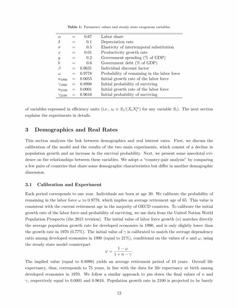
Table 1: Parameter values and steady state exogenous variables.
α = 0.67 Labor shareδ = 0.1 Depreciation rateσ = 0.5 Elasticity of intertemporal substitutionx = 0.01 Productivity growth rateg = 0.2 Government spending (% of GDP)b = 0.6 Government debt (% of GDP)β = 0.9631 Individual discount factorω = 0.9778 Probability of remaining in the labor forcen1990 = 0.0055 Initial growth rate of the labor forceγ1990 = 0.8998 Initial probability of survivingn2100 = 0.0001 Initial growth rate of the labor forceγ2100 = 0.9616 Initial probability of surviving
of variables expressed in efficiency units (i.e., st ≡ St/(XtNwt ) for any variable St). The next section
explains the experiments in details.
3 Demographics and Real Rates
This section analyzes the link between demographics and real interest rates. First, we discuss the
calibration of the model and the results of the two main experiments, which consist of a decline in
population growth and an increase in the survival probability. Next, we present some anecdotal evi-
dence on the relationships between these variables. We adopt a “country-pair analysis” by comparing
a few pairs of countries that share some demographic characteristics but differ in another demographic
dimension.
3.1 Calibration and Experiment
Each period corresponds to one year. Individuals are born at age 20. We calibrate the probability of
remaining in the labor force ω to 0.9778, which implies an average retirement age of 65. This value is
consistent with the current retirement age in the majority of OECD countries. To calibrate the initial
growth rate of the labor force and probability of surviving, we use data from the United Nation World
Population Prospects (the 2015 revision). The initial value of labor force growth (n) matches directly
the average population growth rate for developed economies in 1990, and is only slightly lower than
the growth rate in 1970 (0.77%). The initial value of γ is calibrated to match the average dependency
ratio among developed economies in 1990 (equal to 21%), conditional on the values of n and ω, using
the steady state model counterpart
ψ =1− ω
1 + n− γ.
The implied value (equal to 0.8998) yields an average retirement period of 10 years. Overall life
expectancy, thus, corresponds to 75 years, in line with the data for life expectancy at birth among
developed economies in 1970. We follow a similar approach to pin down the final values of n and
γ, respectively equal to 0.0001 and 0.9616. Population growth rate in 2100 is projected to be barely
12

positive and the dependency ratio is expected to reach almost 58%, which returns a value of γ equal
to 0.9616 in the final steady state. The average retirement period therefore increases to 26 years, and
overall life expectancy rises to 91.
This “representative” transition for developed economies masks some heterogeneity among coun-
tries. For example, Japan is at one extreme of the range, with population growth rates currently in
negative territory, and life expectancy well above 80. At the opposite end of the spectrum, the United
States has a population growth rate just below 1% and life expectancy well below 80. This range is
projected to remain roughly stable throughout the current century.
The other parameters of the model are fairly standard in the literature. The elasticity of intertem-
poral substitution σ is set to 0.5, consistent with the estimates in Hall (1988) and Yogo (2004). The
labor share of output α equals 0.667 and the depreciation rate δ is set to 0.1, in line with the average
post-war values for several advanced economies. Total factor productivity grows at 1% per year, higher
than for the average TFP growth rate for G7 economies post-1990 (0.3%) but close to the value in a
broader sample of OECD countries. Government spending represents 20% of GDP while government
debt corresponds to 60% of GDP. These values are close to their data counterparts for G7 countries
post-1990 (19.2% and 52.3% respectively). Finally, the individual discount factor β is chosen so that
the real interest rate in the initial steady state equals 4%, close to the average ex-post real interest
rate on short-term (maturity less than a year) government bonds for the sample of countries in Figure
1.
The main experiment consists of computing the transition from the initial steady state in 1990 to
the final steady state in 2100. Demographic variables are the only exogenous drivers of the simulation.8
We assume that nt and γt follow
nt = n1990 exp(unt − vnt),
γt = γ1990 exp(uγt − vγt).
where uit and vit (for i = n, γ) are stationary AR(1) processes with common innovation εit. We
choose the persistence parameters ρi and the initial innovation (the only unanticipated shock) such
that the implied process for population growth and the dependency ratio roughly match the data.
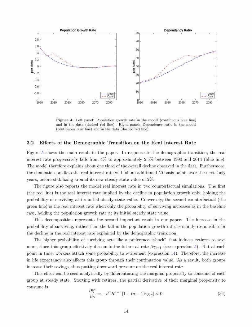
Figure 4 compares the evolution of the exogenous demographic variables in the model with their
empirical counterparts. The left panel shows that, except for a short-lived bump, the assumed process
fits the evolution of population growth in the data very closely. The right-hand side panel shows that
the dependency ratio in the model is smoother than in the data, although very close for the first
thirty years and the last twenty years of the sample. Given that the processes in the model aim at
fitting projections, not actual data, our approach is rather conservative. In particular, the implied
probability of surviving that we back out of the dependency ratio in the model corresponds to a slower
aging profile than the United Nations projections currently imply. As we shall see in the next section,
this approach leads to an underestimation of the effect of the demographic transition on the real
interest rate. In this respect, our results represent a lower bound for the effects of the demographic
transition on the real interest rate.
8The solution is obtained with the shooting algorithm in Dynare.
13
1990 2010 2030 2050 2070 2090
per
cent
-1
-0.8
-0.6
-0.4
-0.2
0
0.2
0.4
0.6
0.8
1Population Growth Rate
ModelData
1990 2010 2030 2050 2070 2090
per
cent
0
10
20
30
40
50
60
70
80Dependency Ratio
ModelData
Figure 4: Left panel: Population growth rate in the model (continuous blue line)and in the data (dashed red line). Right panel: Dependency ratio in the model(continuous blue line) and in the data (dashed red line).
3.2 Effects of the Demographic Transition on the Real Interest Rate
Figure 5 shows the main result in the paper. In response to the demographic transition, the real
interest rate progressively falls from 4% to approximately 2.5% between 1990 and 2014 (blue line).
The model therefore explains about one third of the overall decline observed in the data. Furthermore,
the simulation predicts the real interest rate will fall an additional 50 basis points over the next forty
years, before stabilizing around its new steady state value of 2%.
The figure also reports the model real interest rate in two counterfactual simulations. The first
(the red line) is the real interest rate implied by the decline in population growth only, holding the
probability of surviving at its initial steady state value. Conversely, the second counterfactual (the
green line) is the real interest rate when only the probability of surviving increases as in the baseline
case, holding the population growth rate at its initial steady state value.
This decomposition represents the second important result in our paper. The increase in the
probability of surviving, rather than the fall in the population growth rate, is mainly responsible for
the decline in the real interest rate explained by the demographic transition.
The higher probability of surviving acts like a preference “shock” that induces retirees to save
more, since this group effectively discounts the future at rate βγt+1 (see expression 5). But at each
point in time, workers attach some probability to retirement (expression 14). Therefore, the increase
in life expectancy also affects this group through their continuation value. As a result, both groups
increase their savings, thus putting downward pressure on the real interest rate.
This effect can be seen analytically by differentiating the marginal propensity to consume of each
group at steady state. Starting with retirees, the partial derivative of their marginal propensity to
consume is∂ξr
∂γ= −βσRσ−1 [1 + (σ − 1)εR,γ ] < 0, (34)
14

1990 1993 1996 1999 2002 2005 2008 2011 2014
perc
enta
ge p
oint
s
2.4
2.6
2.8
3
3.2
3.4
3.6
3.8
4
4.2Real Interest Rate
Baseline Population Growth Life Expectancy
Figure 5: Simulated real interest rate following (i) the full demographic transition(blue line), (ii) only the decrease in the population growth rate (red line), (iii) onlythe increase in the probability of surviving (green line).
where εR,γ ≡ (∂R/R)/(∂γ/γ) < 0 is the elasticity of the real interest rate with respect to the prob-
ability of surviving. The first term captures the direct effect discussed above. The second one is the
general equilibrium effect, as the marginal propensity to consume itself depends on the real interest
rate. In this respect, the assumption that the elasticity of intertemporal substitution is smaller than
one is important. With the logarithmic version of Epstein-Zin preferences (which corresponds to the
case σ = 1), only the direct effect survives. And if the elasticity of intertemporal substitution were
assumed to be larger than one, the general equilibrium effect would partially offset the direct one.
Using the implicit function theorem, we can also derive the effect of a change in life expectancy on
the marginal propensity to consume of workers
∂ξw
∂γ= −
βσ(ΩR)σ−1[(σ − 1)εR,γ −
(Ω−ω
Ω
)εξr,γ
]γ[1 + βσ(ΩR)σ−1
(Ω−ω
Ω
)1ξw
] < 0,
where Ω − ω = (1 − ω)ξr/ξw > 0 and εξr,γ ≡ (∂ξr/ξr)/(∂γ/γ) < 0 because of (34) above. The
assumption that the elasticity of intertemporal substitution is smaller than one, while not crucial,
strengthens the result also in this case.
The two top panels of Figure 6 show the quantitative importance of the effect of an increase in the
probability of surviving on the marginal propensity to consume of workers and retirees respectively.
15

1990 1995 2000 2005 2010
pe
r ce
nt
4.5
5
5.5
6Workers MPC
1990 1995 2000 2005 2010
pe
r ce
nt
8
9
10
11
12Retirees MPC
1990 1995 2000 2005 2010
pe
rce
nt
of
GD
P
43.1
43.2
43.3
43.4
43.5Workers Consumption
1990 1995 2000 2005 2010
pe
rce
nt
of
GD
P
5.95
6
6.05
6.1
6.15
6.2Retirees Consumption
1990 1995 2000 2005 2010
pe
r ce
nt
16
17
18
19
20
21Distribution of Wealth
1990 1995 2000 2005 2010
pe
rce
nt
of
GD
P
49
49.2
49.4
49.6
49.8Consumption
Figure 6: Simulated marginal propensity to consume for workers (top left) andretirees (top right), consumption for workers (middle left) and retirees (middle right),distribution of wealth (bottom left), and aggregate consumption (bottom right), inresponse to the increase in the probability of surviving.
The marginal propensity to consume of retirees remains higher than the workers’ one, but it falls
by more (about one fourth against one sixth). Retirees, however, hold more assets, therefore their
consumption falls less (middle panels). In fact, the larger decline in the marginal propensity to
consume of retirees implies that their asset accumulation is proportionally larger than for workers, so
that the distribution of wealth shifts in favor of the former group (top right panel). In the aggregate,
consumption falls by about half a percentage point (bottom right panel). Therefore, the demographic
transition—and in particular the higher probability of surviving– does not carry large consequences for
macroeconomic aggregates. Rather, it is the real interest rate that bears the bulk of the adjustment.
16

The other notable aspect of the demographic transition is the fall in the population growth rate.
As mentioned, the repercussions for the real interest rate are quantitatively less significant than those
of the increase in life expectancy. The intuition is that a falling population growth rate brings about
two effects working in opposite directions. On the one hand, a lower population growth rate reduces
the pool of workers, thus increasing the capital-labor ratio. Therefore, the rental rate decreases, and,
by no arbitrage, so does the real rate. On the other hand, however, a lower population growth rate
progressively increases the dependency ratio—the ratio of retirees to workers. Because retirees have a
larger marginal propensity to consume, this effect tends to offset the consequence of the less efficient
use of capital. Overall, the effect is negative, but quantitatively small. This finding is therefore
consistent with the view that the negative effects of the demographic transition on the real interest
rate may be small and temporary (see, for example, Erfurth and Goodhart, 2014). However, this
conclusion neglects the key role of the increase in life expectancy that this paper highlights.9
3.3 Suggestive Anecdotal Evidence
The model just presented suggests different possible links between demographics and real interest rates.
Here we resort to country-pair comparisons to provide some anecdotal evidence of these relationships
in the data. The key result from the model is that the demographic transition—and, in particular, the
increase in life expectancy—drives the decline in real interest rate observed during the last two and
half decades. Therefore, in the data, we compare how the short-term real interest rate varies for pairs
of countries that differ only in terms of life expectancy, either actual or projected. We want to stress
that this exercise is purely illustrative, and by no means aims to provide definitive empirical evidence
on these patterns.
To perform our analysis, we consider data for two base years, 1990 and 2005. In particular, we
calculate five-year averages, centered at 1990 and 2005, of the short-term real interest rate and life
expectancy. To calculate the projected change in life expectancy, we consider the United Nations
forecast for life expectancy in two 15-year windows, between 1990 and 2005 (as of 1990), and 2005
and 2020 (as of 2005).10
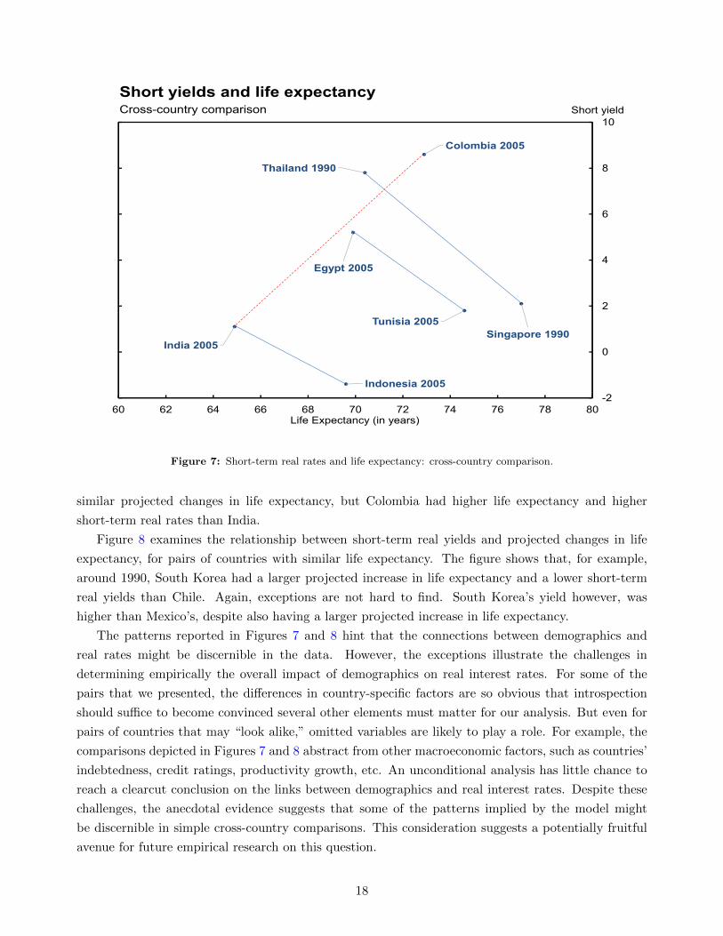
Figure 7 reports the first set of country-pairs. The figure shows short-term real rates and life
expectancy for pairs of countries with similar projected change in life expectancy at the indicated base-
year. For example, in 1990, Thailand and Singapore had similar projected change in life expectancy,
but differed in their short term rates and life expectancy. Singapore had higher life expectancy and
lower short-term yields. Similar patterns hold for other country-pairs, such as Egypt-Tunisia in 2005,
and India-Indonesia in the same year. All three pairs of countries featured similar projected changes
in life expectancy, and the country with higher life expectancy also had lower short-term real interest
rates. Obviously, we can easily find exceptions. For example, the comparison between India and
Colombia in 2005, deviates from the pattern highlighted above. In 2005, Colombia and India had
9Our paper focuses on the savings margin. Recent results on the detrimental effects of lower population growthon labor supply and participation rates (Fujita and Fujiwara, 2014), and on innovation (Aksoy et al., 2015) are thuscomplementary to our work. Eggertsson and Mehrotra (2014) show how a decline in population growth rate can beequivalent to a tightening of borrowing constraints, and thus reduce the equilibrium real interest rate.
10For all country-pairs reported in this exercise, the two countries in each comparison also have similar old dependencyratios (calculated as five-year averages centered at 1990 and 2005).
17
Colombia 2005
Singapore 1990
Thailand 1990
India 2005
Indonesia 2005
Egypt 2005
Tunisia 2005
-2
0
2
4
6
8
10
60 62 64 66 68 70 72 74 76 78 80
Cross-country comparisonShort yields and life expectancy
Life Expectancy (in years)
Short yield
Figure 7: Short-term real rates and life expectancy: cross-country comparison.
similar projected changes in life expectancy, but Colombia had higher life expectancy and higher
short-term real rates than India.
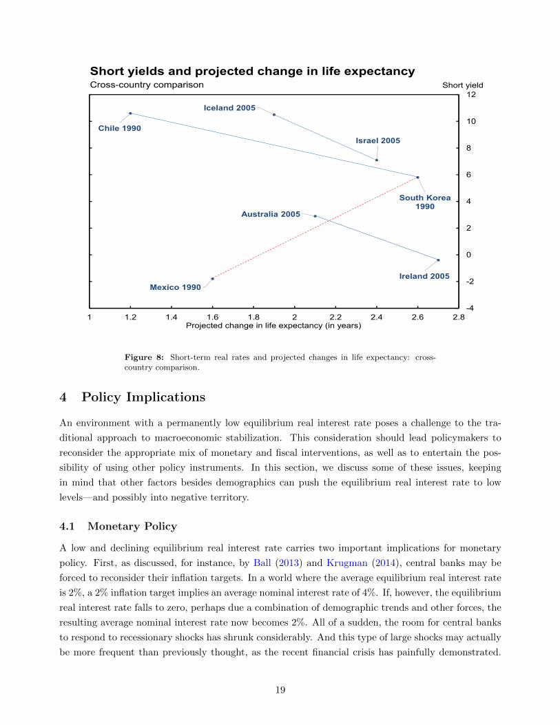
Figure 8 examines the relationship between short-term real yields and projected changes in life
expectancy, for pairs of countries with similar life expectancy. The figure shows that, for example,
around 1990, South Korea had a larger projected increase in life expectancy and a lower short-term
real yields than Chile. Again, exceptions are not hard to find. South Korea’s yield however, was
higher than Mexico’s, despite also having a larger projected increase in life expectancy.
The patterns reported in Figures 7 and 8 hint that the connections between demographics and
real rates might be discernible in the data. However, the exceptions illustrate the challenges in
determining empirically the overall impact of demographics on real interest rates. For some of the
pairs that we presented, the differences in country-specific factors are so obvious that introspection
should suffice to become convinced several other elements must matter for our analysis. But even for
pairs of countries that may “look alike,” omitted variables are likely to play a role. For example, the
comparisons depicted in Figures 7 and 8 abstract from other macroeconomic factors, such as countries’
indebtedness, credit ratings, productivity growth, etc. An unconditional analysis has little chance to
reach a clearcut conclusion on the links between demographics and real interest rates. Despite these
challenges, the anecdotal evidence suggests that some of the patterns implied by the model might
be discernible in simple cross-country comparisons. This consideration suggests a potentially fruitful
avenue for future empirical research on this question.
18
South Korea 1990
Mexico 1990
Iceland 2005
Israel 2005
Ireland 2005
Chile 1990
Australia 2005
-4
-2
0
2
4
6
8
10
12
1 1.2 1.4 1.6 1.8 2 2.2 2.4 2.6 2.8
Cross-country comparisonShort yields and projected change in life expectancy
Projected change in life expectancy (in years)
Short yield
Figure 8: Short-term real rates and projected changes in life expectancy: cross-country comparison.
4 Policy Implications
An environment with a permanently low equilibrium real interest rate poses a challenge to the tra-
ditional approach to macroeconomic stabilization. This consideration should lead policymakers to
reconsider the appropriate mix of monetary and fiscal interventions, as well as to entertain the pos-
sibility of using other policy instruments. In this section, we discuss some of these issues, keeping
in mind that other factors besides demographics can push the equilibrium real interest rate to low
levels—and possibly into negative territory.
4.1 Monetary Policy
A low and declining equilibrium real interest rate carries two important implications for monetary
policy. First, as discussed, for instance, by Ball (2013) and Krugman (2014), central banks may be
forced to reconsider their inflation targets. In a world where the average equilibrium real interest rate
is 2%, a 2% inflation target implies an average nominal interest rate of 4%. If, however, the equilibrium
real interest rate falls to zero, perhaps due a combination of demographic trends and other forces, the
resulting average nominal interest rate now becomes 2%. All of a sudden, the room for central banks
to respond to recessionary shocks has shrunk considerably. And this type of large shocks may actually
be more frequent than previously thought, as the recent financial crisis has painfully demonstrated.
19

A natural approach to counter this undesirable side-effect of the demographic transition on monetary
policy is to raise the inflation target. However, the benefits of higher inflation must be weighted against
its welfare costs, such as those stemming from higher price dispersion (e.g., Ascari and Sbordone 2014).
A second implication is perhaps slightly more subtle. In the baseline three-equation New Keynesian
model (Clarida et al., 1999; Woodford, 2003), optimal monetary policy requires the nominal interest
rate to track at each point in time the so-called “efficient real interest rate”. While specific details
may differ, this result generalizes to most frameworks with nominal rigidities. In this class of models,
the efficient real interest rate is the real interest rate that would prevail absent nominal rigidities and
markup shocks—that is, the real interest rate that arises in a frictionless environment. In the baseline
model, the efficient real interest rate is a combination of technology and preference shocks. In larger
frameworks, other exogenous disturbances (e.g. the investment-specific technology shock) also affect
this variable.
The key point is that all the aforementioned structural shocks are typically assumed to be sta-
tionary. As this paper demonstrates, the demographic transition induces variations in the efficient
real interest rate that are instead likely to be permanent, especially those associated with the increase
in life expectancy. These permanent developments have to be taken into account by the Central
Bank. Carvalho and Ferrero (2014) explore this connection between demographic developments and
monetary policy in an application to Japan, using the same framework as in this paper augmented
with nominal rigidities. Their calibration to the Japanese demographic transition induces a fall in the
efficient real interest rate between two and three percentage points between 1990 and 2014. If the
central bank fails to adjust the nominal interest rate to the low frequency movements in the efficient
real interest rate induced by demographics, monetary policy is systematically too tight, and deflation
arises in equilibrium. Quantitatively, the model can account for the persistence of Japanese deflation
since the early 1990s.
4.2 Fiscal Policy
Whether to bailout banks or to provide economic stimulus (or both), governments of several advanced
and emerging market economies responded to the GFC with expansionary fiscal policies. As a conse-
quence, current levels and projected paths of public debt relative to GDP have notably shifted upward
and are projected to remain high for the next few years (Figure 9). Should this increase in debt
become permanent, this policy would—perhaps unintentionally—counterbalance some of the effects of
the demographic transition on real rates. For example, Summers (2014) has recently been an advocate
of debt-financed spending, pushing the idea that, in a secular stagnation environment, government
demand can substitute for private demand.
We can use our model to find the increase in the level of debt to GDP required to undo the effects
demographics on the equilibrium real interest rate. In the final steady state of our simulations, the
real interest rate stabilizes around 2%. The comparative statics exercise involves keeping the ratio
of government spending to GDP at 20%, and finding the level of debt to GDP that brings the real
interest rate back to 4%. In our calibrated model, the debt-to-GDP ratio can reach 210% before the
real interest rate returns to 4%.
20

2001 2004 2007 2010 2013 2016 2019
% o
f GD
P
0
50
100
150Net Government Debt
FranceIrelandItalyJapanSpainUnited KingdomUnited States
Figure 9: Ratio of net government debt to GDP. Sample: France, Ireland, Italy,Japan, Spain, United Kingdom and United States. Source: IMF World EconomicOutlook Database April 2015.
Our calculations are arguably an upper bound on the required debt expansion, because the sim-
ulations do not take into account the increase in risk premia that are typically associated with large
increases in government indebtedness, as the recent experience in the European periphery suggests.
At the same time, however, the model returns a value of debt to GDP that is not too far from the
levels currently observed in Japan—a country where the consequences of high levels of debt for risk
premia appear to be very modest, but where the effects of the demographic transition are most visible.
4.3 Structural Reforms
This section considers two types of “structural reforms” that can contribute to directly increase the
equilibrium real interest rate. The first is an unspecified reform that increases the growth rate of
productivity—which is a parameter in the model. The second is an increase in the (average) retirement
age, which is also controlled by a parameter in the model—the probability of retirement.
So far, in our simulations, we have kept the value of productivity growth fixed at 1%. This number
is actually on the high side for the largest advanced economies in the world. Recently, the literature
has been debating to which extent the secular stagnation hypothesis could also involve a supply-side
element. For example, Gordon (2012) suggests that the period between 1750 and 2000 may have been
unique in the history of economic growth, thanks to several inventions that dramatically changed the
21
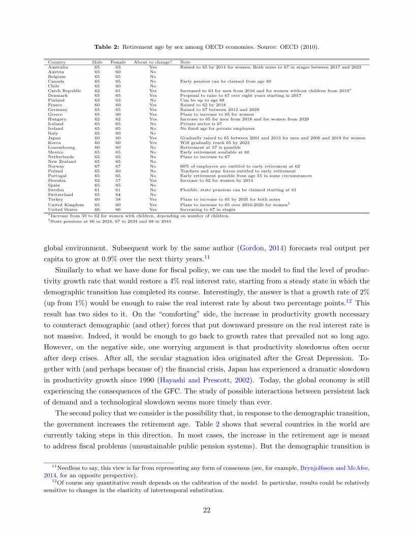
Table 2: Retirement age by sex among OECD economies. Source: OECD (2010).
Country Male Female About to change? NoteAustralia 65 63 Yes Raised to 65 by 2014 for women; Both sexes to 67 in stages between 2017 and 2023Austria 65 60 NoBelgium 65 65 NoCanada 65 65 No Early pension can be claimed from age 60Chile 65 60 NoCzech Republic 62 61 Yes Increased to 63 for men from 2016 and for women without children from 2019∗
Denmark 65 65 Yes Proposal to raise to 67 over eight years starting in 2017Finland 63 63 No Can be up to age 68France 60 60 Yes Raised to 62 by 2018Germany 65 65 Yes Raised to 67 between 2012 and 2029Greece 65 60 Yes Plans to increase to 65 for womenHungary 62 62 Yes Increase to 65 for men from 2018 and for women from 2020Iceland 65 65 No Private sector is 67Ireland 65 65 No No fixed age for private employeesItaly 65 60 NoJapan 60 60 Yes Gradually raised to 65 between 2001 and 2013 for men and 2006 and 2018 for womenKorea 60 60 Yes Will gradually reach 65 by 2023Luxembourg 60 60 No Retirement at 57 is possibleMexico 65 65 No Early retirement available at 60Netherlands 65 65 No Plans to increase to 67New Zealand 65 65 NoNorway 67 67 No 60% of employees are entitled to early retirement at 62Poland 65 60 No Teachers and army forces entitled to early retirementPortugal 65 65 No Early retirement possible from age 55 in some circumstancesSlovakia 62 57 Yes Increase to 62 for women by 2014Spain 65 65 NoSweden 61 61 No Flexible, state pensions can be claimed starting at 61Switzerland 65 64 NoTurkey 60 58 Yes Plans to increase to 65 by 2035 for both sexes
United Kingdom 65 60 Yes Plans to increase to 65 over 2010-2020 for women†
United States 66 66 Yes Increasing to 67 in stages∗Increase from 59 to 62 for women with children, depending on number of children.†State pensions at 66 in 2024, 67 in 2034 and 68 in 2044.
global environment. Subsequent work by the same author (Gordon, 2014) forecasts real output per
capita to grow at 0.9% over the next thirty years.11
Similarly to what we have done for fiscal policy, we can use the model to find the level of produc-
tivity growth rate that would restore a 4% real interest rate, starting from a steady state in which the
demographic transition has completed its course. Interestingly, the answer is that a growth rate of 2%
(up from 1%) would be enough to raise the real interest rate by about two percentage points.12 This
result has two sides to it. On the “comforting” side, the increase in productivity growth necessary
to counteract demographic (and other) forces that put downward pressure on the real interest rate is
not massive. Indeed, it would be enough to go back to growth rates that prevailed not so long ago.
However, on the negative side, one worrying argument is that productivity slowdowns often occur
after deep crises. After all, the secular stagnation idea originated after the Great Depression. To-
gether with (and perhaps because of) the financial crisis, Japan has experienced a dramatic slowdown
in productivity growth since 1990 (Hayashi and Prescott, 2002). Today, the global economy is still
experiencing the consequences of the GFC. The study of possible interactions between persistent lack
of demand and a technological slowdown seems more timely than ever.
The second policy that we consider is the possibility that, in response to the demographic transition,
the government increases the retirement age. Table 2 shows that several countries in the world are
currently taking steps in this direction. In most cases, the increase in the retirement age is meant
to address fiscal problems (unsustainable public pension systems). But the demographic transition is
11Needless to say, this view is far from representing any form of consensus (see, for example, Brynjolfsson and McAfee,2014, for an opposite perspective).
12Of course any quantitative result depends on the calibration of the model. In particular, results could be relativelysensitive to changes in the elasticity of intertemporal substitution.
22
often the deep cause of such fiscal imbalances. As life expectancy increases, social security agencies
need to pay pensions to individuals for a longer period of time. Obviously, this problem is more
severe in defined-benefit systems of advanced economies, where shrinking generations of workers are
responsible for the pensions of larger pools of retirees. In this paper, we abstract from the fiscal
dimension, as individuals save for their own retirement and the government balances the budget given
a stream of exogenous (wasteful) spending.13
We assume that the government increases the retirement age by manipulating the probability
to retire ω, and we perform a comparative static exercise similar to the ones for fiscal policy and
productivity. An increase of two years in the retirement age—a typical reform currently being imple-
mented in advanced economies—leads to a rather modest rise (10 basis points) in the real interest rate.
Conversely, the reform that fully offsets the decline in the real interest rate due to the demographic
transition would be enormous, requiring an average employment period of 105 years.14 While this
result is obviously unrealistic, the overall message of the exercise is clear. While structural reforms
that increase the retirement age go in the right direction to compensate the negative effects of the
demographic transition on the real interest rate, these policies should not be used in isolation.
5 Conclusion
The demographic transition that all advanced economies are currently experiencing is one key element
that explains the prolonged decline of global real interest rates. The main channel through which
demographics affect real interest rate is the increase in life expectancy. At all stages of their life
cycle, individuals save more to finance consumption over a longer time horizon. Quantitatively, the
demographic transition can account for about one third of the overall decline in the real interest rate
since 1990. We have provided some anecdotal evidence that the data support the importance of this
channel, and discussed several policy implications.
Going forward, our research agenda on this topic consists of fully exploring the empirical dimen-
sion of this question, revisiting historical episodes of the connection between low interest rates and
demographic changes, and studying its political-economic consequences.
13Gertler (1999) introduces social security benefits for retirees in his model.14A more sensible implementation of this reform would consist of indexing the retirement age to life expectancy,
perhaps through periodic revisions. Yet, the elasticity of the indexation scheme would still need to be quite high.
23

References
Acemoglu, D. and S. Johnson (2007). Disease and Development: The Effect of Life Expectancy on
Economic Growth. Journal of Political Economy 115, 925–985.
Aksoy, Y., H. Basso, R. Smith, and T. Grasl (2015). Demographic Structure and Macroeconomic
Trends. Unpublished, Birkbeck College.
Ascari, G. and A. M. Sbordone (2014). The macroeconomics of trend inflation. Journal of Economic
Literature 52 (3), 679–739.
Ball, L. (2013). The Case For Four Percent Inflation. Central Bank Review 13, 17–31.
Blanchard, O. (1985). Debt, Deficits and Finite Horizons. Journal of Political Economy 93, 223–247.
Brynjolfsson, E. and A. McAfee (2014). The Second Age Machine. Norton.
Carvalho, C. and A. Ferrero (2014). What Explains Japan’s Persistent Deflation? Unpublished, PUC
Rio.
Chen, K., A. Imrohoroglu, and S. Imrohoroglu (2009). A Quantitative Assessment of the Decline in
the U.S. Current Account. Journal of Monetary Economics 56, 1135–1147.
Clarida, R., J. Galı, and M. Gertler (1999). The Science of Monetary Policy: A New Keynesian
Perspective. Journal of Economic Literature 37, 1661–1707.
Eggertsson, G. and N. Mehrotra (2014). A Model of Secular Stagnation. NBER Working Paper 20574.
Epstein, L. and S. Zin (1989). Substitution, Risk Aversion, and the Temporal Behavior of Consumption
and Asset Returns: A Theoretical Framework. Econometrica 57, 937–969.
Erfurth, P. and C. A. Goodhart (2014, November). Demography and Economics: Look Past the Past.
VoxEU.org.
Farmer, R. (1990). Rince Preferences. Quarterly Journal of Economics 105, 43–60.
Ferrero, A. (2010). A Structural Decomposition of the U.S. Trade Balance: Productivity, Demograph-
ics and Fiscal Policy. Journal of Monetary Economics 57, 478–490.
Fujita, S. and I. Fujiwara (2014). Aging and Deflation: Japanese Experience. Unpublished, Federal
Reserve Bank of Philadelphia.
Gertler, M. (1999). Government Debt and Social Security in a Life-Cycle Economy. Carnegie-Rochester
Conference Series on Public Policy 50, 61–110.
Gordon, R. (2012). Is U.S. Economic Growth Over? Faltering Innovation Confronts the Six Headwinds.
NBER Working Paper 18315.
24
Gordon, R. (2014). The Demise of U.S. Economic Growth: Restatement, Rebuttal, and Reflections.
NBER Working Paper 19895.
Hall, R. E. (1988). Intertemporal Substitution in Consumption. Journal of Political Economy 96,
339–357.
Hansen, A. (1939). Economic Progress and Declining Population Growth. American Economic Re-
view 29 (1), 1–15.
Hayashi, F. and E. Prescott (2002). The 1990s in Japan: A Lost Decade. Review of Economic
Dynamics 5, 206–235.
Kreps, D. and E. Porteus (1978). Temporal Resolution of Uncertainty and Dynamic Choice Theory.
Econometrica 46, 185–200.
Krugman, P. (2014). Four Observations on Secular Stagnation. In Secular Stagnation: Facts, Causes
and Cures, Chapter 4, pp. 61–68. VoxEU.org.
Nishimura, K. (2011). Population Ageing, Macroeconomic Crisis and Policy Challenges. Panel at the
75th Anniversary Conference of Keynes’ General Theory. University of Cambridge, UK.
Obstfeld, M. and K. Rogoff (1996). Foundations of International Macroeconomics. MIT Press.
Summers, L. H. (2014). Reflections on the New Secular Stagnation Hypothesis. In Secular Stagnation:
Facts, Causes and Cures, Chapter 1, pp. 27–38. VoxEU.org.
Woodford, M. (2003). Interest and Prices: Foundations of a Theory of Monetary Policy. Princeton
University Press.
Yaari, M. (1965). Uncertain Lifetime, Life Insurance, and the Theory of the Consumer. Review of
Economic Studies 32, 137–150.
Yogo, M. (2004). Estimating the Elasticity of Intertemporal Substitution When Instruments Are
Weak. The Review of Economics and Statistics 86, 797–810.
25

A Model Solution
A.1 Retirees
The first-order conditions with respect to capital and government bonds are, respectively,
(Crt (j, τ))ρ−1 = βγt+1
(V rt+1 (j, τ)
)ρ−1 ∂Vrt+1 (j, τ)
∂Krt (j, τ)
(Crt (j, τ))ρ−1 = βγt+1
(V rt+1 (j, τ)
)ρ−1 ∂Vrt+1 (j, τ)
∂(Brt (j, τ))
The envelope conditions, used to obtain the Euler equations for the retiree’s problem, are
∂V rt (j, τ)
∂Krt−1 (j, τ)
= (V rt (j, τ))1−ρ (Crt (j, τ))ρ−1 R
Kt + (1− δ)
γt
∂V rt (j, τ)
∂(Brt−1 (j, τ))
= (V rt (j, τ))1−ρ (Crt (j, τ))ρ−1 Rt−1
γt.
Combining the two sets of optimality conditions yields the standard Euler equations for bonds and
capital
1 = βRtπt+1
[Crt+1(j, τ)
Crt (j, τ)
]− 1σ
= β[RKt+1 + (1− δ)
] [Crt+1(j, τ)
Crt (j, τ)
]− 1σ
. (35)
To solve the problem of retirees, guess that consumption is a fraction of total wealth
Crt (j, τ) = ξrt
(Rt−1A
rt−1(j, τ)
γt
). (36)
Substitution into the Euler equation (35) yields a law of motion for the marginal propensity to consume
of a retiree ξrt
ξrt+1
(RtA
rt (j, τ)
γt+1
)= (βRt)
σ ξrt
(Rt−1A
rt−1(j, τ)
γt
). (37)
Substitution of the guess (36) into the budget constraint of a retiree (10) leads to the expression below
for the dynamics of asset holdings
Art (j, τ) = (1− ξrt )Rt−1A
rt−1(j, τ)
γt.
Combining the last expression with the law of motion for the marginal propensity to consume of a
retiree (37) yields the first-order non-linear difference equation for ξrt (12) in the text.
Moreover, conjecture that the value function is linear in consumption
V rt (j, τ) = ∆r
tCrt (j, τ) . (38)
26
Then, from (5), it must be the case that
(∆rtC
rt (j, τ))ρ = (Crt (j, τ))ρ + βγt+1
(∆rt+1C
rt+1 (j, τ)
)ρ.
Substituting for consumption at t+ 1 from (35) and simplifying yields
(∆rt )ρ = 1 + γt+1β
σ (Rt)σ−1 (∆r
t+1
)ρ.
From (12), it then follows that the proportionality term in (38) is
∆rt = (ξrt )
σ1−σ .
A.2 Workers
The first-order condition for workers’ asset holdings is
(Cwt (j))ρ−1 = β[ωt+1V
wt+1 (j) + (1− ωt+1)V r
t+1 (j, t+ 1)]ρ−1[
ωt+1∂V w
t+1 (j)
∂Awt (j)+ (1− ωt+1)
∂V rt+1 (j, t+ 1)
∂Awt (j)
].
The envelope conditions are for the worker’s problem are
∂V wt (j)
∂Awt−1 (j)= (V w
t (j))1−ρ (Cwt (j))ρ−1Rt−1
and∂V r
t (j, t)
∂Awt−1 (j)=
∂V rt (j, t)
∂Art−1 (j, t)
∂Art−1 (j, t)
∂Awt−1 (j)=
∂V rt (j, t)
∂Art−1 (j, t),
where the last equality follows from (7)—i.e., from the initial conditions of the retirees’ optimization
problem.
Combining the first order condition with the envelope conditions yields an Euler equation for
workers of cohort j
(Cwt (j))ρ−1 = βRt[ωt+1V
wt+1 (j) + (1− ωt+1)V r
t+1 (j, t+ 1)]ρ−1[
ωt+1
(V wt+1 (j)
)1−ρ (Cwt+1 (j)
)ρ−1+ (1− ωt+1)
(V rt+1 (j, t+ 1)
)1−ρ (Crt+1 (j, t+ 1)
)ρ−1]. (39)
To solve the problem of workers, conjecture that their value function has the same form as (38)
V wt (j) = ∆w
t Cwt (j) . (40)
27
Substituting this guess back into the Euler equation (39) together with (38) leads to
(Cwt (j))ρ−1 = βRt[ωt+1∆w
t+1Cwt+1 (j) + (1− ωt+1) ∆r
t+1Crt+1 (j, t+ 1)
]ρ−1[ωt+1
(∆wt+1
)1−ρ+ (1− ωt+1)
(∆rt+1
)1−ρ]. (41)
Defining the adjustment term Ωt ≡ ωt + (1− ωt)(
∆rt
∆wt
)1−ρ, the Euler equation becomes
ωt+1Cwt+1 (j) + (1− ωt+1)
(∆rt+1
∆wt+1
)Crt+1 (j, t+ 1) = (βΩt+1Rt)
σ Cwt (j) . (42)
The guess for the decision rule of a worker is
Cwt (j) = ξwt(Rt−1A
wt−1 (j) +Hw
t
), (43)
where human wealth Hwt is defined in (22).
From (11), the decision rule for a retiree born in period j who just left the labor force is
Crt (j) = ξrtRt−1Awt−1 (j) .
Substituting the last expression into the Euler equation yields
ωt+1
(Awt (j) +
Hwt+1
Rt
)+ (1− ωt+1)
(∆rt+1
∆wt+1
)εt+1A
wt (j) =
(βΩt+1)σ (Rt)σ−1 ξwt
ξwt+1
(Rt−1A
wt−1 (j) +Hw
t
),
where εt ≡ ξrt /ξwt . Using the definition of Ωt, the last expression becomes
Awt (j) +ωt+1H
wt+1
Ωt+1Rt+1= βσ (Ωt+1Rt)
σ−1 ξwtξwt+1
(Rt−1A
wt−1 (j) +Hw
t
). (44)
Moreover, from the budget constraint of a worker and the guess (43), we obtain the law of motion for
worker j’s wealth
Awt (j) +ωt+1H
wt+1
Ωt+1Rt= (1− ξwt )
(Rt−1A
wt−1 (j) +Hw
t
).
Substituting this result back into the Euler equation (44), it follows that the marginal propensity to
consume for a worker evolves according to expression (18) in the text.
Finally, the original guess of the value function (19) is valid if
(∆wt C
wt (j))ρ = (Cwt (j))ρ + β
[ωt+1∆w
t+1Cwt+1 (j) + (1− ωt+1) ∆r
t+1Crt+1 (j, t+ 1)
]ρ.
The last equation, combined with (42), yields
(∆wt )ρ = 1 + βσ (Ωt+1Rt)
σ−1 (∆wt+1
)ρ.
28

Expression (18) then implies that
∆wt = (ξwt )
σ1−σ .
Hence, the ratio of the proportionality factors in the value function is ∆rt+1/∆
wt+1 = ε
−(1/ρ)t and
Ωt = ωt + (1− ωt) ε1
1−σt .
29