Demographic Uncertainty and Welfare in a Life-cycle Model

CAEPR Working Paper #2008-024

Demographic Uncertainty and Welfare in a Life-cycle Model under Alternative Public

Pension Systems

M Saifur Rahman Indiana University Bloomington

September 19, 2008

This paper can be downloaded without charge from the Social Science Research Network electronic library at: http://ssrn.com/abstract=1270643. The Center for Applied Economics and Policy Research resides in the Department of Economics at Indiana University Bloomington. CAEPR can be found on the Internet at: http://www.indiana.edu/~caepr. CAEPR can be reached via email at [email protected] or via phone at 812-855-4050.

©2008 by M Saifur Rahman. All rights reserved. Short sections of text, not to exceed two paragraphs, may be quoted without explicit permission provided that full credit, including © notice, is given to the source.

Demographic Uncertainty and Welfare in a Life-cycle Modelunder Alternative Public Pension Systems

M Saifur Rahman�

Indiana University at BloomingtonEmail: [email protected]

September 8, 2008

Abstract

In this paper, I analyze consumption, aggregate savings,output and welfare implications of�ve di¤erent social security arragements whenever there is demographic uncertanity. FollowingBohn(2002), I analyze the e¤ect of an uncetain population growth in an extended version ofa modi�ed Life-cycle model developed by Gertler(1999). Population growth dampens savingsand output under all arrangements. Pay-as-you-go-De�ned Bene�t system appears to farebetter than all other alternatives, falling short of the private annuity market with no pensionsystem. But social security in general increases social welfare, with Fully Funded systemsfaring the best. Thus there appears to be a clear tradeo¤ bewteen growth and social welfare.The social security system also reduces the volatility of the economy.JEL Classi�cation: E21, E62, E64, H23, H24, H41, H55, J18, J26Keywords: Demographic uncertainty, Social welfare, Life-cycle model, Annuity market,

Pay-as-you-go, Fully funded, De�ned bene�t, De�ned contribution.

1 Introduction

In this paper,I analyzed consumption, aggregate savings, output behavior and also welfare undertwo popular social security arrangements when ever there is demographic uncertainty. The twopopular social security arrangements are Pay as You Go(PAYGO) and Fully Funded(FF) socialsecurity. I analyze two variants of each of these social security systems, the De�ned Bene�t(DB)and the De�ned Contribution(DC) arrangements. Under the assumtption of a �xed bene�t ratefor the DB system and a �xed tax rate for the DC system, I analyze both short run and long rune¤ect of demographic uncertainty. I use a life-cycle model to carry out my analysis. In this setup,the population is divided into two groups, workers and retirees. These two groups are heteroge-nous in terms of their consumption and savings behavior. All the workers and all the retireeswould be ex-ante identical. In the model there is uncertainty about retirement and death. Iassume the transitional probability to retirement and death to be constant. In order to introduceshort run variation, I introduce a stochastic population growth process for the workers. I con-sider a permanent increase in the growth rate of the worker population. Longrun analysis revealscontrasting e¤ect of alternative social security system on the consumption, capital accumulation

�Contact address:Department of Economics,Indiana University at Bloomington,Phone:812-855-0179,email:[email protected]. I would like to thank my Third year paper committee members, EricLeeper, Michael Kaganovich, and Brian Peterson for their valuable suggesstions during my research. I would liketo specially thank Hess Chung for his critical suggestions, thorough guidence and helpful scrutini of my work. Iwould also like to acknowledge helpful comments from James Murray and Michael Plante. Finally, I thank all theparticipants of the Spring 2007 Macroeconomics Brown Bag workshop. All errors are mine

1

and output. Social security arrangement appears to be in general bene�cial for the retiree, butharmful to the worker�s consumption. Pension system also dampens output growth and discour-ages savings. PAYGO-DB appears to fare better than rest of the arrangements, although farworse than the private annuity market without social security or government intervention. Thiscontrasts with the existing literature. In case of the population shock, it appears that Inter-generational risk sharing mechanism like the PAYGO systems provide better risk sharing. Butwhen social welfare is considered, there appears to be clear trade-o¤ between growth and welfare.FF system appears to be welfare maximizing, even when compared with the non distortionaryprivate annuity market. In fact the latter performs the worst in terms of welfare. I also look atspeed of convergence of the economy and relate that to the volatility of the system. It appearsthat social security arrangements in general reduces the volatility of the economy.

2 Motivation and Literature Review

In this paper, my plan is to look at the e¤ect of a permanent shock in the growth rate of thework force on the economy under alternative social security systems using a new kind of lifecyclemodel. Figure 1-5 highlights some of the demographic features and trends in employment inUSA. There are several interesting things in the that. First, although population growth hasslowed down after the 70�s, with unemployment rate at its lowest and with a rapid increasingrate of immigration fueled by positive signal from the policy makers, USA has been experiencinga large in�ux of fresh and returning entrant into the labor force. An increased immigration to theUSA and similar increase in the number of naturalization of aliens de�nitely have contributed tothe improved performance of employment scenario over the changes in the labor force. This isprojected to remain at a higher level. Hence analyzing the e¤ect of an increases in the growth rateof workforce force may be a useful exercise. The second motivation comes from the changes in thenature of retirement in USA. Using HRS data, Quinn(1999) estimates that between one-thirdand one -half of older Americans take on Bridge Jobs(temporary, sometimes lower paid jobs)before exiting labor force completely. He concludes that retirement pattern in America are muchricher and more varied than the stereotypical one-step view of retirement suggests. Maestas(2004)�nds that more than one-third of retirees in their 50�s go back to work after retirement. Using alarger panel data set from the HRS survey, Cahill, Giandrea and Quinn(2005) �nds that (Table1 in appendix) in 1992, 15% of all the employed worker since age 49 had part time employment.In 2002, in the same population(now ten years older), 25% of all employed men had part timejobs. In 2000, this fraction was even larger, 33%. We also see similar picture for female. Table-2reveals some more dramatic results. Out of the men who had full time job in 1992, 40% ofthem in 2002 who then over 60 years of age had part time job. Out of the people who were65 years and older(full retirement age in traditional sense) 37.5 % had part time job. Twoimportant conclusions arise from their �ndings. First, retirees should no longer be modeled aswithdrawing completely from the labor force. Second, it is safe to assume that the part time jobsthat traditional retirees get after their retirement pays them a lower e¤ective wage.

In the literature, life-cycle models are popular for analyzing demographic transition. Eversince the development of the life-cycle models by Brumberg, Ando, Modigliani(1956), these mod-els have been extensively used by both policy makers and researchers. With the popularizationof Discrete Stochastic General Equilibrium(DSGE) models, there has been attempts to developa DSGE version of life-cycle model. To my knowledge, the �rst of such model was developedby Gali(1990) which tried to �nd evidence of life cycle behavior in a DSGE model by adoptingthe Blanchard-Yarri model. But in order to avoid problems with aggregation, he assumed anidentical(and constant) MPC for the workers and the retirees. Clarida(1991) was able to developa DSGE life cycle model where he was able to achieve aggregation without assuming constant oridentical MPC for all cohorts. My model is very close to Gertler(1999). He developed a DSGE

2

life-cycle model which was a modi�ed version of Blachard-Yarri(1965) model where he added atransitional probability to retirement in addition to the original generational index parameter, thetransitional probability to death. Gertler�s model has di¤erent MPC�s for di¤erent groups. Basedon his assumption on the preference structure, Gertler argued that all the works have identicalMPC and all the retirees have same MPC. He was then able to aggregate all the consumptionfunctions of workers of di¤erent age and did the same thing for all the retirees. This allowedhim to derive an aggregate consumption function for the workers and also for the retirees. Healso developed aggregate human and non-human wealth functions for the economy and carriedout various �scal experiments. Recently Ferrero(2005), Kilponen, Kinnunen and Ripatti(2006),Keuschigg and Keuschigg(2004), Roeger(2005), Kara and Thadden(2006), Fujivara and Teran-ish(2006), Grafenhofer, Jaag and Keuschigg(2006) have extended the Gertler(1999) model furtherand studied di¤erent aspects of population ageing in their models. The main advantages of usingGertler�s framework is that one can apply various tools used in the Real Business Cycle literatureand analyze not only the stationary equilibrium, but also the transition path. But perhaps themost popular Life cycle simulated models were developed by Auerbach and Kotilioko¤(1987) .While analysis of debt in a representative agent might be misleading1, the analysis based on thesimulated life cycle models does not o¤er any analytical tractability. Second, other than fewauthors such as Kotiliko¤, most of the researchers focus on various ways to make the existingPAYGO system more e¢ cient. A comparative analysis of major alternative social security systemis nearly absent. Kotliko¤, Smetters and Walliser(1999) analyzes the e¢ cacy of alternative pri-vatized social security systems using their famous simulated A-K model. De Nardi,·Imrohoro¼gluand Sargent(1999) on the other hand analyzes the impact of various �scal policy measures tothe retirement of the baby boomers under the present social security system. Finally, the workclosest to my paper are Bohn(2002, 1999, 1998) which carry out a comparative analysis of variousalternative social security and debt management schemes using an OLG framework. Althoughhis analysis provides signi�cant insight into the e¢ cacy of alternative policy regime, the OLGframework limits its applicability for policy analysis. In a two period stochastic OLG framework,although Bohn uses several RBC tools that I will also employ, I will be able to analyze the entiretransition path of the economy before and after a demographic shock which the former was notable to do. The short run e¢ cacy of alternative policy regime is equally important for policymakers. This paper will therefore be a value addition to that literature. My model is also dif-ferent from the original work by Gertler(1999). His model has social security in the form of alump-sump tax-transfer scheme. This is clearly unrealistic, as Gertler himself acknowledges. Mymodel will have full speci�cation of various social security regimes. My paper also di¤ers fromGertler(1999) in terms of policy analysis. Gertler focuses mainly on various �scal experiments likechanging the government debt. He also conducts some demographic experiments like changingthe dependency ratio by experimenting on transitional probability of death and experimentingon the transition to retirement. My experiments will be di¤erent because I will focus only onintroducing demographic shock to the growth rate of the workforce. Although my experimentswill have similar e¤ect on the dependency ratio as Gertler, the source of that is di¤erent. Finally,I will completely obstruct away from introducing any government debt in my model, which is thedriving force in Gertler�s experiments.

Keeping in mind the above mentioned issues, I plan to develop a DSGE Life cycle modelwith a fully developed social security system. I would like to incorporate some fundamentaluncertainties that were outlined in Bohn(2002) and Gertler(1999). In my model, I would liketo analyze how basic uncertainties are shared by the workers and the retirees under alternativesocial security arrangement. My basic model would be an extended version of Gertler(1999). Tointroduce life-cycle factors but maintain tractability, Gertler made two kinds of modi�cations of

1Romer(1989) suggested that government debt might have very little e¤ect on the real activity in the Blan-chard/Weil framework. Gertler(1999) argues that adding life cycle features would enhance the impact

3

the Blanchard/Weil framework. First, Gertler introduced two stages of life: work and retirement.Gertler then imposed a constant transition probability per period for a worker into retirement, aswell as a constant probability per period of death for a retiree. In my model, both the transitionprobability per period of death and retirement would be stochastic with both following an iidprocess . Second, Gertler employed a class of non-expected utility preferences proposed by Krepsand Porteus(1978) and later popularized by Farmer (1990), Weil(1990) and Epstein and Zin(1990)that generate certainty-equivalent decision rules in the presence of income risk. Gertler showedthat with these two modi�cations it is possible to derive aggregate consumption/savings relationsfor workers and for retirees. It is also possible to express the current equilibrium values of allthe endogenous variables as functions of just two predetermined variables: the capital stock andthe distribution of nonhuman wealth between retirees and workers. In my model, I will focuson the aggregate behavior of the Workers and the Retirees separately and keep track of theevolution of their human(wage income) and non-human(income from savings on capital asset)wealth. Because the model permits realistic average periods of work and retirement, the modelis useful for quantitative policy analysis in a way that complements the use of large-scale models.The advantage of this framework is its parsimonious representation, which helps make clear thefactors that underlie the results. In particular, it is possible to obtain an analytical solution foraggregate consumption behavior, conditional on the paths of wages and interest rates. In thiscase with variable work e¤ort, it is also possible to �nd an analytical solution for aggregate laborsupply. Since the e¤ects of government and social security on the economy in this frameworkwork their way through consumption and labor supply, these (partial) analytical solutions willhelp clarify the nature and strength of the policy transmission mechanisms. Further, becauseof its parsimony, it is straightforward to integrate this life-cycle setup into existing growth andbusiness-cycle models in order to study a much broader set of issues which have already beenstarting to be analyzed by many researchers.

3 Basic feature of the Life-cycle model

In this model, individuals have �nite lives and they evolve through two distinct stages of life:work and retirement. To derive a tractable aggregate consumption function and at the sametime permit realistic (average) lengths of work and retirement, I make three kinds of assump-tions. These assumptions involve: (1) population dynamics; (2) insurance arrangements; and (3)preferences.

3.1 Demographic feature

The population dynamics will follow a natural ordering to allow for tractability of our model.Consumers are assumed to be born as workers. Workers face a constant retirement probability!:Conditional on being a worker in the current period, the probability of remaining one in thenext period is !; while the probability of retiring is 1 � !. These transition probabilities areindependent on individual�s employment tenure. Once an individual has retired he is facing aperiodic probability of death 1 � . The survival probability is assumed to be independent ofretirement tenure. Let us denote Nw

t and Nrt to be the total number of workers and retirees. In

period t+ 1;I assume that there would be (1 + nt+1 � !)new workers born, where nt is anotherwhite noise process with mean n and a variance �2. Hence the workers�population follows thefollowing law of motion:

Nwt+1 = (1 + nt+1 � !)Nw

t + !Nwt = (1 + nt+1)N

wt (1)

The retiree population follows law of motion:

4

N rt+1 = (1� )N r

t + (1� !)Nwt (2)

De�ne t =Nrt

Nwtto be the ratio of retiree to the worker, the dependency ratio. Using equa-

tion(1) and (2), we can show that the dependency ratio follows law of motion:

t+1(1 + nt+1) = t + (1� !) (3)

By using equation(3) we can drive the following:

Nwt+1

Nwt

= (1 + nt+1) (4)

N rt+1

N rt

= (1 + nt+1) t+1 t

(5)

Nt+1Nt

= (1 + nt+1)1 + t+11 + t

(6)

lnnt+1 = �n lnnt + e1t+1, 0 < �n < 1 (6.a)

Where Nt is the total population at time t which is simply de�ned as follows

Nt = N rt +N

wt (6.b)

Furthermore, in the stationary equilibrium, t+1 = t = , nt+1 = n. Then Nwt+1,N

rt+1 and

Nt+1 all grow at the same rate n and the population dynamics in this model is stationary.

3.2 Insurance Market

To eliminate the impact of uncertainty about time of death, I introduce a perfect annuitiesmarket, following Yaari (1965) and Blanchard (1985). The annuities market provides perfectinsurance against this kind of uncertainty. Under the arrangement, each retiree e¤ectively turnsover his wealth to a mutual fund that invests the proceeds. The fraction of those that surviveto the next period receive all the returns, while the (estates of) the fraction 1� who die receivenothing. Each surviving retiree receives a return that is proportionate to his initial contributionof wealth to the mutual fund. Thus, for example, if Rt+1 is the gross return per dollar investedby the mutual fund, the gross return on wealth for a surviving retiree is Rt+1 :

3.3 Preference

Now the timing of economic decisions are very important. Each persons make all his decisionsat the beginning of time, all his decisions are ex-ante.Now we will de�ne the utility function ofan individual who derives utility from consumption, c and leisure (1 � l). Following Kreps andPorteus(1978), and Farmer(1990), we will use a special class CES non-expected utility function.The parametric form of the utility function will be following Weil(1990)

V zt (at�1) =

�U(czt ; l

zt )� + �zt+1Et

hVt+1(at) j z

i ��

� 1�

(7)

This preference structure has the convenient property of separating between the elasticity ofinter temporal substitution given by � = 1

(1��) and the coe¢ cient of relative risk aversion, given

5

by �: Following Gertler(1999) and Ferrero(2005), we assume � = 1:Then equation (8) can bewritten as:

V zt (at�1) =nU(czt ; l

zt )� + �zt+1Et

hVt+1(at) j z

i�o 1�

(8)

According to Farmer(1990), These preferences generate certainty-equivalent decisions rules in theface of idiosyncratic income risk, in contrast to standard Von-Neumann/Morgenstern utility func-tions. Roughly speaking, because preferences are over the mean of next period�s value function,individuals only care about the �rst moment of expected income in deriving their decision rules)2.On the other hand, they do care about smoothing consumption over time. The curvature para-meter � introduces a smooth trade-o¤ for individuals between consuming today versus consumingtomorrow. In analogy to the standard case, the desire to smooth consumption implies a �niteinter temporal elasticity of substitution , given by � = 1

(1��) . Thus a virtue of the preferencestructure is that it permits �exibility over the choice of �, which is a key parameter in deter-mining the quantitative e¤ects of debt and social security. Furthermore, Weil(1990) argues thatthe value of � determines people�s attitude towards intertemporal substitution, or inter temporalconsumption smoothing. � < 1 means Income e¤ects are smaller than Substitution e¤ect andvice versa for � > 1:This certainty-equivalent analysis clari�es the respective role of risk aversionand inter temporal substitution. The substitution e¤ect depresses the marginal propensity tosave as soon as agents are risk averse, as the optimum way to maintain the original utility levelwhen wage income risk increases is to consume more today (and thus avoid facing the increasedrisk). The income e¤ect is simply a precautionary savings e¤ect, whose magnitude depends onthe inter temporal elasticity of substitution: increased wage risk implies a higher probability oflow consumption tomorrow, against which consumers will protect themselves the more, by con-suming less, the more averse they are to inter temporal �uctuations of consumption. Which ofthese two con�icting e¤ects dominates depends on the strength of the precautionary motive, i.e.,on the magnitude of the inter temporal elasticity of substitution.

Finally, we assume the period utility function is Cobb-Douglas. With that the recursive utilityfunction of the agents in the model:

V zt (at�1) =n�(Czt )

v (1� lzt )1�v��+ �zt+1Et

hVt+1(at) j z = w; r

i�o 1�

(9)

Where:

Et

hVt+1(at j w)

i= !V wt+1 + (1� !)V rt+1 , �wt+1 = � (10)

Et

hVt+1(at j r)

i= V rt+1, �

rt+1 = � (11)

Therefore, this preference representation now has conveniently separated period elasticity ofsubstitution v and inter temporal elasticity of substitution � for consumption.

Now I will proceed to solve the optimization problem by both the worker and the retiree.Both worker and retiree have 1 unit of time which they allocate between work(l) and leisure.Both receive the same wage Wt:But the retirees are less productive than the worker, which willbe re�ected by a productivity parameter �:

2Since retirees do not face any income risk, they behave as if they had standard Von- Neumann/Morgensternpreferences. In other words, the solution to their decision problem is the same as if they had standard preferences.

6

4 Model with Private Annuity Market

In the baseline mode, we will consider optimization by the agents without any government inter-vention. There will only be an annuity market .

4.1 Optimization by the Retiree

Retirees consume out of asset income and labour income. In general, one can index each retireeby the time he was born j and the time he left the labor force k. Ultimately, it will not benecessary to keep track of how assets and consumption are distributed among retirees over j andk. Under my assumptions one can simply aggregate across di¤erent cohorts. Let Arjkt and Crjktbe the assets at the beginning of time t and consumption at t, respectively, of a retired personwho was born at time jand left the labor force at time k; and let Rtbe the gross return on assetsfrom period t � 1 to t. For a retiree at t who participates in a perfect annuities market, hisoptimization problem looks like:

V rjkt (Art�1)fCrjk;lrjkg

=nh�

Crjkt

�v(1� lrjkt )1�v

i�+ �

�V rt+1 (A

rt )��o 1

�(12)

Subject to:

Arjkt =RtA

rjkt�1

+Wt�lrjkt � Crjkt (13)

With 0 � � � 1:Following Gertler(2000),the consumer�s optimization has to satisfy additional conditions. The

�rst one is as follows:

limi!1

Et iRt+iA

rjkt+i�1

iQj=1

Rt+j

= 0 (14)

The above equation is meant to rule out Ponzi schemes. The individual has to satisfy anintertemporal budget constraint. He eventually has to pay o¤ any debt, he cannot continuouslyplay with Ponzi schemes. As it turns out, the above condition is not su¢ cient. We need a strongercondition for optimization under uncertainty. The in�nite horizon budget constraint now has tohold in expectations. It has to hold both in ex-ante and ex-post sense since the individual isallowed to borrow only at riskless rate. It has to hold for every possible realization of Wt andRt which are essentially random variables. Thus the individual can borrow risklessly but has tobe able to pay back the debt. Therefore, the optimization problem of retiree has to satisfy thefollowing intertemporal budget constraint:

Et

266641Xi=0

iCrjkt+iiQj=1

Rt+j

37775 = RtArjkt�1

+Hrjkt (15)

Where Hrjkt is the expected lifetime labor income of the retiree de�ned later.

We also need the following requirement:

lim Eti!1

fRt+ig =�R, lim Et

i!1fWt+ig =

�W (16)

7

Where the last condition is a stationary condition on the fWtg1t=0process.

The �rst order condition with respect Crt along with respective envelope conditions3 yields

the following euler equation for the retiree:

Crjkt+1 =

"�Wt+1

Wt

��(1�v)(�Rt+1)

#�Crjkt (17)

The �rst order condition with respect to lrjkt along with respective envelope conditions yieldsthe following conditions:

lrjkt = 1� �

�WtCrjkt (18)

where� =

1� vv

(19)

In order to derive a decision rule for the retiree we employ Modigliani(1963) idea that a personconsumes a fraction of this life time income. Therefore, I guess that the consumption functionlooks like:

Crjkt = �t(RtA

rjkt�1

+Hrjkt ) (20)

Where �t is the marginal propensity to consume(MPC) out of life income for the retiree. Art�1

is the total non-human asset accumulated up to time t and Hrt is the expected lifetime labour

income for the retiree, which is given by:

Hrjkt =

1Xn=0

nWt+n�lrjkt+n

nQz=0

Rt+z+1

= �Wtlrt +

Hrjkt+1

Rt+1(21)

We will also guess the following form for the vrt ,

V rjkt = �rtCrjkt

��

�Wt

�1�v(22)

After some math, we can prove the following:

�rt = (�t)�1� (23)

Also, the MPC follows the following law of motion:

�t = 1��

Wt

Wt+1

��(1�v)��R��1t+1

�t�t+1

(24)

4.2 Optimization by the Worker

The worker�s maximization problem looks like:

V wjkt (Awt�1)fCwjk;lwjkg

=nh�

Cwjkt

�v(1� lwjkt )1�v

i�+ �

h!V wt+1

�Awjkt

�+ (1� !)V rt+1

�Aw

rjkt

�i�o 1�(25)

3For a detailed derivation, please see the appendix 1

8

Subject to:

Awjkt = RtAwjkt�1 +Wtl

wjkt � Cwjkt (26)

Awrjk

t = RtAwjkt�1 � C

wjkt (27)

where the second budget constraint is for the worker who was worker today(t) but will becomeretiree tomorrow(t + 1). As a result, this new retiree was not able to put his wealth into theannuity market. Also, when the workers of period t retires at period t+1, he will no longer havehis labour income as a worker.

Similar to the retiree, we need Ponzi constraint for the worker which looks like:

limi!1

EtRt+iA

wjkt+i�1

iQj=1

t+iRt+j

= 0 (27.a)

Where t+i is an additional factor that is used to weight the gross interest rate, to be de�nedlater. This will along with equation(16) give us an intertemporal budget constraint for the workerwhich looks like:

Et

266641Xi=0

Cwjkt+i

iQj=1

t+iRt+j

37775 = RtAwjkt�1 +H

wjkt (27.b)

The problem of the worker is quite complicated and the �rst order conditions are messy. Inorder to simplify our calculation, We will guess that the consumption function looks like:

Cwjkt = �t(RtAwjkt�1 +H

wjkt ) (28)

Where �t is the marginal propensity to consume out of life income for the worker. Awjkt�1 is

the total non-human asset accumulated up to time t and Hwjkt is the expected lifetime labour


Hwjkt =Wtl

wjkt +

!Hwjkt+1

t+1Rt+1+(1� !)Hrjk

t+1

t+1Rt+1(29)

where:

t+1 = ! + (1� !)�1

1��t+1 (30)

where:

�t+1 =�t+1�t+1

(31)

and �t follows the following law of motion:

�t = 1��

Wt

Wt+1

�(1�v)��(Rt+1t+1)

��1 �t�t+1

(32)

Now we will guess a functional form for V wjkt :

9

V wjkt = �wt Cwjkt

��

Wt

�1�v(33)

The �rst order condition with respect to Cwjkt along with respective envelope conditions andequation(30)yields the following euler equation:

!Cwjkt+1 + (1� !)� (�t+1)�

1�� Crjkt+1 = (34)"�Wt

Wt+1

��(1�v)��Rt+1

n! + (1� !)� (�t+1)

�1��o 11��

#�Cwjkt

where:

� =

�1

�

�1�v(35)

Finally, the �rst order condition for lwjkt looks like

lwjkt = 1� �

WtCwjkt (36)

4.3 Derivation of Aggregate Functions

If we look at the consumption functions for a workers, we see two things. First, the MPC attime period t will be the same for all the workers. Second, The only thing that will di¤er istheir lifetime accumulated income which will vary with each cohort. We can therefore, proceedto aggregate the consumption for all the workers for a given period t. We will �rst drop all thej and k subscript and derive some more aggregate variables:

Total labor supply by workers

Lwt =NwPi=0

lwt (i) =NwPi=0

�1� �

WtCwt (i)

�= Nw

t �NwPi=0

�

WtCwt (i) = Nw

t ��

WtCwt (37)

Total labour supply by the retirees:

Lrt =NrPi=0

lrt (i) = N rt �

NrPi=0

�

�WtCrt (i) = N r

t ��

�WtCrt (38)

The aggregate e¤ective labour supply to the economy:

Lt = Lwt + �Lrt (39)

Aggregate non-human wealth by all worker at time t:

Awt�1 =NwPi=0

Awt�1(i) (40)

The aggregate life time labor income of the workers at time t

Hwt =WtL

wt +

!Hwt+1

(1 + nt+1) t+1Rt+1+

(1� !)Hrt+1

(1 + nt+1) t+1Rt+1 t+1(41)

10

By summing up the individual guess function for Consumption, we can derive the aggregateconsumption function for workers

Cwt = �t(RtAwt�1 +H

wt ) (42)

Similarly, we can derive aggregate relationships for the retirees:

Crt = �t(RtArt�1 +H

rt ) (43)

Hrt = �WtL

rt +

Hrt+1 t

Rt+1 t+1(44)

The aggregate wealth of the economy for the workers and the retirees look like:

Art = Art�1Rt + �WtLrt � Crt � (1� !)

�Awt�1Rt +WtL

wt � Cwt

�(45)

Awt = !�Awt�1Rt +WtL

wt � Cwt

�(46)

Ct = Cwt + Crt (47)

Let us de�ne At�1 as the aggregate wealth of the economy at period t and �t�1 =Art�1At�1

as the

share of the asset held by the retirees. It also follows that 1� �t�1 =Awt�1At�1

. Using these two andalso equation (41) and (42)we can rewrite the aggregate wealth of the economy as follows

At

��t!� 1� !

!

�= Rt�t�1At�1 + �WtL

rt � Crt (48)

Finally, using the de�nition of the aggregate wealth, equation (38) and (39) looks like:

Cwt = �t [Rt (1� �t�1)At�1 +Hwt ] (49)

Crt = �t [Rt�t�1At�1 +Hrt ] (50)

4.4 Production side of the economy

Production is subject to a neoclassical production function with labour augmenting technologicalprogress:

Yt = (XtLt)�K1��

t�1 (1)

where the technology follows an AR(1) process:

lnXt+1 = �x lnXt + e1t+1; 0 < �x < 1 (2)

The wage rate and return on capital are determined as:

Wt = �YtLt

(53)

Rt = (1� �)YtKt�1

+ (1� �) (54)

11

Capital evolves according to the following law of motion:

Kt = Yt � Ct + (1� �)Kt�1 (55)

Finally we close the model by specifying the relationship between the capital stock and thewealth4:

Kt = At 8 t (56)

4.5 De�nition of Competitive Equilibrium

A competitive equilibrium is a sequence of endogenous predetermined variables {Kt�1; Art�1; Awt�1}

and a sequenceof endogenous variables f�t; �t;t;Hr

t ;Hwt ; C

wt ; C

rt ;Wt; Rt; A

wt ; A

rtg, that satisfy equations 37-

56, given the sequence of the exogenous predetermined variables {Nt+1, Xt+1} speci�ed by (6)and (59), and given the initial values of all the predetermined variables, Kt, At, Nt, and Xt.

5 Model with PAYGO-De�ned Bene�t Social Security System

In the PAYGO model we will consider optimization where there is a PAYGO social securitysystem for the retiree. The role of the government will be to carry out this transfer to the presentretirees by taxing the present workers. The government will impose a payroll tax on the workers.The retirees, although working, are not subject to the payroll tax. The bene�t which will includea participation rate which will determine how much transfer the retirees receive will be �xed inthe de�ned bene�t case. The above two are assumptions of the model where the former is madeto simplify the solution of the model and the latter is a speci�cation used in the literature. Theincome of the retirees will still be annuitized so that accidental bequest is prevented.


The optimization problem by the retiree looks very similar to the baseline case except for thefact that the retirees now also receive a social security payment Erjkt = BWt, where B is a �xedde�ned bene�t rate, or the participation rate. For a retiree at t who participates in a perfectannuities market, his optimization problem looks like:


=nh�

Crjkt


i�+ �

�V rt+1 (A

rt )��o 1

�(57)

Subject to:

4 In order to see that equation(56) holds, lets add up equation (45) and (46), and we getArt +A

wt = Rt (A

rt�1 +A

wt�1) +Wt (�L

rt + L

wt )� Crt � Cwt

Using the fact that, At�1 = Art�1 +Awt�1 for t and t� 1 and equation (39), and substituting the value of Rt and

Wt from equation (53) and (54), the above equation can be written as:At = (1� �) Yt

Kt�1At�1 + (1� �)Kt�1 + �

YtLtLt ��Crt � Cwt

Now if Kt�1 = At�1, then the above equation can be written as:At = Yt + (1� �)Kt�1 � Crt � CwtWhere the right hand side of the eqaution is identical to the right hand side of equation (55). Therefore,Kt = At

12

Arjkt =RtA

rjkt�1

+Wt�lrjkt � Crjkt +BWt (58)

With 0 � � � 1:Similar to the private annuity market case, the retirees will have a Ponzi constraint like

equation(14). Their intertemporal budget constraint now looks like:

Et

266641Xi=0

iCrjkt+iiQj=1

Rt+j

37775 = RtArjkt�1

+Hrjkt + Srjkt (58.a)

Where Srjkt is expected lifetime social security payment to the retiree, to be de�ned later.The �rst order condition with respect Crt along with respective envelope conditions yields verysimilar Euler equation for the retiree:

Crjkt+1 =

"�Wt

Wt+1

��(1�v)(�Rt+1)

#�Crjkt (59)

The �rst order condition with respect to lrjkt along with respective envelope conditions yieldsthe following conditions:

lrjkt = 1� �

�WtCrjkt (60)

where � is de�ned in equation(18)Similar to the baseline case, I guess that the consumption function looks like:

Crjkt = �t(RtA

rjkt�1

+Hrjkt + Srjkt ) (61)

Where �t is the marginal propensity to consume(MPC) out of life income for the retiree. Art�1

is the total non-human asset accumulated up to time t and Hrt is the expected lifetime labour

income for the retiree, de�ned in equation (21) and Srjkt is the expected lifetime social securitypayment which is given by:

Srjkt =

1Xv=0

vErt+vNrt+v

vQz=0

Rt+z+1

=ErtN rt

+ Srjkt+1Rt+1

(62)

Lets explain the term on the right hand side of the equation (62). Ert+v = N rt+vBWt+v is the

total social security payments that all the retirees expect to get paid at some period in the futuret+ v:In order to get the individual transfer, we divide it by the total retiree population in periodt + v:This individual payment is conditional on the fact that the retiree survives up to periodv. That is why v is multiplied with the individual transfer. Finally, we have to discount thetransfer to get the present value all future social security payment. This explains the discountingterm in the denominator.

We will also have similar guess of the following form for the vrt ,

V rjkt = �rtCrjkt

��

�Wt

�1�v(63)

Where we can again prove that

13

�rt = (�t)�1� (64)

Finally, the MPC follows the same law of motion as with the baseline case

�t = 1��

Wt

Wt+1

��(1�v)��R��1t+1

�t�t+1

(65)


The worker�s problem would also be similar except now he has to pay a payroll tax on his wageincome. We will assume that the worker pays a constant payroll tax � on his wage income. Theworker�s maximization problem looks like:


=nh�

Cwjkt


i�+ �

h!V wt+1

�Awjkt

�+ (1� !)V rt+1

�Aw

rjkt

�i�o 1�(66)

Subject to:

Awjkt = RtAwjkt�1 + (1� � t)Wtl

wjkt � Cwjkt (67)

Awrjk


wjkt (68)

where the intuition behind the equation(67) and (68) was explained in the previous section.The Ponzi constraint of the worker is same as the private annuity case. Now the intertemporalbudget constraint looks like the following:

Et

266641Xi=0

Cwjkt+i

iQj=1

t+iRt+j

37775 = RtAwjkt�1 +H

wjkt + Swjkt (68.a)

Where Swjkt is expected lifetime social security payment to the worker, to be de�ned later.We will again guess that the consumption function looks like:


wjkt + Swjkt ) (69)

Where �t is the marginal propensity to consume out of life income for the worker. Awjkt�1 is

the total non-human asset accumulated up to time t and Hwjkt is the expected lifetime labour


Hwjkt =Wtl

wjkt +

!Hwjkt+1

t+1Rt+1+(1� !)Hrjk

t+1

t+1Rt+1(70)

where t+1has been de�ned in the last section. Now Swjkt is the present value of expectedlifetime social security that the workers will receive when they retire. Swjkt will be de�ned asfollows:

Swjkt =

1Xv=0

!v(1�!)Srt+v+1Nrt+v+1

t+v+1Rt+v+1

�t+v+1�t+v+1

vQz=0

Rt+z+1t+z+1

=(1� !)Srt+1N rt+1t+1Rt+1

�t+1�t+1

+!Swjkt+1

t+1Rt+1(71)

14

Lets explain the term on the right hand side of the equation(71). If the worker retires inperiod t+ v+1, he will receive a social security payment of Srt+v+1 divided by the population at

t+ v + 1. So,Srt+v+1

Nrt+v+1t+v+1Rt+v+1

�t+v+1�t+v+1

is the capitalized value of the social security for a worker

who was working at period t+ v and retired at t+ v + 1:In order to receive that social securitypayment, the person has to be a worker up to period t + v and then retires with probability(1�!) at t+v+1. This explains why !v(1�!) is multiplied with the capitalized value. Finally,in order to get the present value of the social security payment at period t, we have discountthis future payment. This explains the discounting factor that appears in the denominator ofequation(71).

The law of motion for �t looks like:

�t = 1��

(1� � t)Wt

(1� � t+1)Wt+1

�(1�v)��(Rt+1t+1)

��1 �t�t+1

(72)

We will have similar guess about the functional form for V wjkt :


��

(1� � t)Wt

�1�v(73)

The �rst order condition with respect to Cwjkt along with respective envelope conditions andequation(30)yields the following Euler equation:

!Cwjkt+1 + (1� !)� (�t+1)�

1�� Crjkt+1 = (74)"�(1� � t)Wt

(1� � t+1)Wt+1

��(1�v)��Rt+1

n! + (1� !)� (�t+1)

�1��o 11��

#�Cwjkt

where� is de�ned in the previous section.Finally, the �rst order condition for lwjkt looks like very similar to the baseline case

lwjkt = 1� �

(1� � t)WtCwjkt (75)


In the case of the PAYGO-DB system, there will be an additional aggregate constraints, thegovernment budget. Following Bohn(2002), the government uses �xed pension bene�t �nancedby a payroll tax on the current workers. Taxes and Bene�ts are conveniently stated in terms ofa payroll tax rate � t and a �xed replacement rate B:Denoting � tWtL

wt real value of aggregate

tax revenue from the worker and Ert = N rt BWt to be the real value of aggregate social security

payment to the retiree, the Government Budget constraint looks like

N rt BWt = � tWtL

wt (76)

In order to derive the rest of the aggregate relationships, we aggregate equations 60-75 ac-cording to their respective populations and get the following

Lwt = Nwt �

�

(1� � t)WtCwt (77)

Lrt = N rt �

�

�WtCrt (78)

15

Cwt = �t [Rt (1� �t�1)At�1 +Hwt + S

wt ] (79)

Crt = �t [Rt�t�1At�1 +Hrt + S

rt ] (80)

Hwt = (1� � t)WtL

wt +

!Hwt+1

(1 + nt+1) t+1Rt+1+

(1� !)Hrt+1

(1 + nt+1) t+1Rt+1 t+1(81)

Hrt = �WtL

rt +

Hrt+1 t

Rt+1 t+1(82)

Srt = N rt BWt +

Srt+1 t(1 + nt+1)Rt+1 t+1

(83)

Swt =(1� !)Nw

t Srt+1

N rt+1t+1Rt+1

�t+1�t+1

+!Swt+1

t+1Rt+1 (1 + nt+1)(84)

At

��t!� 1� !

!


rt � Crt +N r

t BWt (85)

The equations for �t and �t, Kt,Rt, Wt, Xt, t, Nwt , nt+1 and Yt are same as the previous

section.The Production side of the economy did not change. We can therefore proceed to de�ne the

Competitive equilibrium in the PAYGO system


A competitive equilibrium in the PAYGO system is a sequence of endogenous predetermined vari-

ables fKt�1; Art�1; Awt�1g and a sequence of endogenous variables

��t; �t;t;H

rt ;H

wt ; C

wt ; L

rt ; L

wt ;

Crt ;Wt; Rt; Awt ; A

rt

�,

that satisfy equations 76-85 given the sequence of the exogenous predetermined variables { Nt+1,Xt+1} speci�ed by (6) and (59) and a given exogenous rate of payroll tax � , and given the initialvalues of all the predetermined variables, Kt, At, Nt, and Xt.

6 Model with PAYGO-De�ned Contribution Social Security Sys-

tem

The PAYGO-De�ned Contribution will be identical to the De�ned bene�t system except forthe fact that now the contribution will be �xed. Following Bohn(2002) again,the governmentuses pension bene�t �nanced by a �xed payroll tax on the current workers. Taxes and Bene�tsare conveniently stated in terms of a �xed payroll tax rate � and a variable replacement rateBt:Denoting �WtL

wt real value of aggregate tax revenue from the worker and Ert = N r

t BtWt

to be the real value of aggregate social security payment to the retiree, the government budgetconstraint looks like

N rt BtWt = �WtL

wt (86)

The optimization will be identical to the de�ned bene�t case, including the Ponzi contraintsand the intertemporal budget constraints. Most of the aggregate relationships will remain un-changed. The ones that will changed are summarized as follows:

16

Lwt = Nwt �

�

(1� � t)WtCwt (87)

Hwt = (1� �)WtL

wt +

!Hwt+1

(1 + nt+1) t+1Rt+1+

(1� !)Hrt+1

(1 + nt+1) t+1Rt+1 t+1(88)

Srt = N rt BtWt +

Srt+1 t(1 + nt+1)Rt+1 t+1

(89)

At

��t!� 1� !

!


rt � Crt +N r

t BtWt (90)

The de�nition of competitive equilibrium will be identical to the de�ned bene�t case wherethe above new equations has to be satis�ed in equilibrium.

7 Model with Fully Funded-De�ned Bene�t Social Security

In the Fully Funded(FF from now on) de�ned bene�t model we will consider optimization wherethere is a FF social security system for the retiree. This system is di¤erent from the PAYGOsystem in a number of ways. First, under the FF system, a worker pays payroll tax throughouthis working life. Second, this tax revenue is put into a fund where the government invests theproceeds(social security fund). Finally, when the person retires, he receives social security whichwould be the tax revenue he accumulated plus the interest. For simplicity, we will assume theworker pays a payroll tax � t . The retirees again will not be taxed. When the worker movesinto the retirement phase, he will receive the accumulated tax revenue plus interest. Makingretirement bene�t contigent on the life long tax payments throughout working phase is the correctmechanism. But it is very complicated, we will assume that the retirees bene�t is linked to thetaxes paid right before retirement. In this way, the fully funded de�ned bene�t(DB) systemwill be a notional fully funded system where the �nancing formula uses a Bismarckian Rule5,where the pensions are related to the partial earnings history, in our case, the history just beforeretirement.


The optimization problem by the retiree looks very similar to the PAYGO De�ned Bene�t case,including the Ponzi contraints and the intertemporal budget constraints, except for the fact thatthe retirees�social security now depends on the tax collected from the workers previously. For aretiree at t who participates in a perfect annuities market, he chooses Crjk; lrjk to maximize (57)subject to the (58). The �rst order conditions are same as (59) and (60).

Similar to the PAYGO case, I guess that the consumption function looks like:

Crjkt = �t(RtA

rjkt�1

+Hrjkt + Srjkt ) (91)

�t,Art�1 ,H

rt has been de�ned before and S

rjkt is the expected lifetime social security payment

which, although de�ned before, is given by:

5For an elaborate discussion on the Bismarckian rule and other �nancing rule such as the Beveridgean Rule, seeDocquier and Paddison(2003)

17

Srjkt =1Xv=0

vErt+vNrt+v

vQz=0

Rt+z+1

=ErtN rt

+ Srjkt+1Rt+1

(92)

Where Ert+v = N rt+vBWt+v is the aggregate social security payments that all the retirees in

period t receives. We will also have similar guess for the V rt as (63) and condition (89) has to besatis�ed. The MPC of the retirees will also follows the same law of motion as the equation (65)


The worker�s problem would also be similar except now he has to pay a payroll tax on his wageincome. We will assume that the worker pays a constant payroll tax � t on his wage income. Theworker�s will choose Cwjkt ; lwjkt to maximize (66) subject to (67) and (68). We will again guessidentical function for the consumption function as the PAYGO-DB. All the variables have thesame functional form. The law of motion for �t is identical as the PAYGO-DB case. We willhave similar guess about the functional form for V wjkt .The �rst order condition with respect toCwjkt and lwjkt yields identical solutions as the PAYGO-DB case.


Just like the PAYGO-DB system, in the case of the FF-DB system, there will be an additionalaggregate constraint, the government budget. The government distribute social security paymentamong the retirees which will be collected as payroll tax from the workers from the previousperiod. Following Abel(2003) and Karni and Zilcha(1989), denoting � tWt�1Lwt�1 aggregate taxrevenue from the worker from period t�1 and N r

t BWtto be the aggregate social security paymentto the retiree, the Government Budget constraint looks like

N rt BWt =

�� tWt�1L

wt�1�Rt (93)

The capital market clearing condition now looks like:

Kt = Art +Awt + � tWtL

wt 8 t (94)

The rest of the aggregate relationships are identical to equations (77)-(85).


A competitive equilibrium in the FF-DB will be same as the PAYGO-DB where all the previousconditions have to be satis�ed and also equation 93 and 94 are satis�ed.

8 Model with Fully Funded-De�ned Contribution Social Secu-rity

The FF-DC will be identical to the DB system except for the fact that now the contribution willbe �xed. Following Karni and Zilcha(1989) again,the FF-DC budget constraint looks like:

N rt BtWt =

��Wt�1L

wt�1�Rt (95)

All other aggregate relationships will remain unchanged except some whose form will looklike the new set of equations de�ned in case of the PAYGO-DC case.

18

9 Calibration and nature of experiments under di¤erent pension

systems

There are two sources of growth in this economy, the population growth and the technologicalprogress. Thus in steady state all the quantity variables grow at the exogenously given rateof growth of the e¤ective labor force, XtLwt , which is equal to (1 + x)(1 + n) � (1 + x + n).Because there is growth in the steady state, we have normalize each of the choice variables.For Yt;Hr

t ;Hwt ; C

wt ; C

rt ; L

wt ; L

rt ; Lt and Kt�1, we use XtNw

t and for Wt we use Xt as the scalingfactor. Appendix 1,2 and 3 shows the derivation, scaling and the steady state system for theprivate annuity market without social security. The rest of the models are derived in the similarmanner.

Table 1 shows calibrated values of the exogenous parameters used in this paper. The calibra-tion of each of the models is very crucial. It is therefore important to specify the calibration strat-egy very clearly. First, PAYGO-DB will serve as the baseline model for this paper because it is thesystem that operates in existence. In order to calibrate the model to derive steady state values ofour choice variables, I will choose values for the exogenous parameters �; �; ; �; �; !; �; �; x; n and�:The value of and ! are taken from Auerbach and Kotiliko¤(1987). They are chosen so thata person spends 45 years as worker and 10 years as retired.Following Ferrero(2005), individualsare assumed to enter the workforce as workers when they are 20 years old and work on average(1� !)�1 years. The value of the parameter ! = 0:977 is chosen to match a 45-year averagepermanence in the labor force, which corresponds to Auerbach and Kotiliko¤(1987), where thecalibration is done as follows:

(1� !)�1 = 45) ! =44

45= 0:977 (96)

The value of the survival probability of a retiree, is chosen to be 0.80 to match the averageexpected lifetime horizon for a retiree, which is equal to 70 years for the US and EU. The formulaworks as follows:

65 + (1� )�1 = 70) =4

5= 0:80 (97)

Therefore, we use the above mentioned values for the choice parameters. The value of �and � is taken from Cooley(1995). The rest of the variables are taken from Campbell(1994) butcan also be found in Rebelo and King(1988). The value of � and � are the most crucial andcontroversial parameters of the model. I will calibrate them simultaneously along with two otherimportant variables of the model, the social security tax and the replacement rate, or the bene�trate. The choice of using appropriate value for the social security tax and the bene�t rule is veryimportant. Bohn(2002) uses the value of � to be 12.4% and value of the bene�t rate to be bein between 30% and 40%. But unlike him, I have more restriction in my calibration because Ihave to also match the real interest rate for the economy which should be very close to 3%. Iwill choose a plausible value for � so that I get a plausible value for the participation rate. Incase of the PAYGO-DB, I will choose � and � to be 0.50 and 0.96 and the participation rate tobe 24.9%. The system of nonlinear equations in the steady state then will yield a steady statetax rate to be equal to 12.4% which matches with Bohn(2002)6.These two values will serve asthe benchmark values. In case of the DB systems, we will keep the participation rate constant at24.9% and determine the tax rate. In case of the DC systems, we will keep the tax rate constant

6Trying to calibrate the value of participation rate to be equal to 30% and tax rate to be 12.4% and achieve areal interest rate to be close to 3 % was a di¢ cult task and will consider values of � and � which are usually usedin the literature. I will therefore, only use plausible values of them . This will give a real interest rate which isclose to 3%, a tax rate which is 12.4% and a bene�t rate which is close to 30%.

19

at 12.4% and will determine the participation rate. As we will show, in order to get tax rate andparticipation rate under the FF system similar to the the PAYGO, we will assume the value of� to be 0.958 instead of 0.96. For the Private Annuity market, I will use the baseline parameterfrom the PAYGO-DB system. Table-1 reports all the parameter values to be used in the model.

Now the nature of the experiment that I will conduct has to be speci�ed clearly. My ex-periment will look at the impulse response functions and transitional dynamics of the systemswhen there is an unanticipated permanent 1% increase in the growth rate of workforce. I will useGensys algorithm to derive my impulse response functions. My methodology to derive impulse

response of a permanent shock will follow Leeper and Yang(2006). De�ne^Zt = log(

sZtsZ) to be the

log deviation of a variable from its balanced growth trajectories. We then log-linearize the entiresystem of equations and feed in to the Gensys algorithm developed by Sims(2002). After identi-fying that the systems have a unique solution,I proceed to derive the impulse response functionsof the choice variables for a one percent permanent shock to the growth rate of the workforce.The derivation is done in two steps. First, Gensys calculates the initial response of the variablesto the population shock. Next, I iterate on the initial response for 100 periods and derive theimpulse response functions of the variables in the system.

10 Comparison of Performance under di¤erent Social security

Our economic analysis of the economy under alternative pensions systems will be done in sixsteps. First, we will look at performance of the economy under initial steady state of the systemwhen the population is stationary. Second, we will look at the immediate response of the economyof a permanent population shock. Third, we will look at the dynamics of the economy duringthe transition to the new steady state. Fourth, we will compare the economy under initial andnew steady state. Fifth, we will compare the social welfare of the economy before and after thepermanent population shock. Finally, we will simulate our model and compare the volatility ofthe fundamental variables of our model under di¤erent social security regime when there is apopulation shock.

10.1 Analysis of Initial Steady State

Table 2 reports the steady state values of the variables of each of the systems before and after apermanent shock. We see several interesting results. First, In the initial steady state, the MPCfor the retiree is signi�cantly larger than the MPC for the workers under alternative systems.Lower MPC for the worker is a desirable property of my life-cycle model because it is consistentwith the classic lifecycle model predictions of Modigliani(1956) and Harrod(1948). Therefore, themodel passes the �rst acid test because it mimics life-cycle consumption propensity. Second, Theinitial steady state capital is also largest for the perfect annuity model. The PAYGO system hashigher capital than the FF system. The initial steady state capital is also higher under PAYGOfor both the worker and the retiree. Third, Overall, the retirees supply little labor compared tothe workers. In the initial steady state,total labor supply is the largest for the perfect annuitymodel. Worker�s labor supply is lowest under FF system. Retiree�s labor supply is similar underPAYGO or FF and lower than perfect annuity market. According to Feldstein(2005), a perfectannuity market with no social security will surely yield higher capital accumulation when thereis stationary population. This is because social security involves some form of taxation(either�xed or �exible) which distorts savings by the worker. This is evident by a 17% decline in initialsteady state savings(comparing row 9, column 2 and column 5 of table 2) by the worker under

20

PAYGO and a 21% decline in case of FF(comparing row 9, column 2 and column 8 of table2). Again, social security bene�ts(de�ned or �exible) distorts savings by the retiree which washighlighted by Bohn(2002). The disincentive of the retiree to save more results in a 56% reductionin savings under PAYGO and a 62% decline in case of FF. Overall, there is a 11% decline intotal savings under PAYGO and 15% decline under FF. These are much lower compared to a30-50% reduction estimated by Feldstein(1974). But the puzzling fact is that FF yields lowersavings than PAYGO. A closer analysis should resolve this issue. First, notice that the nature ofincome inequality is identical under PAYGO and FF in the initial steady state. Second, retireeslabor supply under these two regimes are almost identical. Hence, total labor supply declinebecause of the decline in worker�s labor supply. With a slightly higher wage in the PAYGOsystems, the retirees enjoy higher labor income than FF. Although rental rate is slightly lowerunder the PAYGO, the workers with much bigger chunk of capital earns a higher capital incomethan the retirees. Finally, since the social security bene�t is same under PAYGO and FF in theinitial steady state(as was the objective of my calibration exercise), the retirees, overall, has lowerincome under FF than under PAYGO. Therefore, PAYGO with higher income for both workersand retirees results in a higher capital accumulation in PAYGO than FF. From the risk sharingperspective of the social security systems, we notice one striking result. In an economy where theretirees work part time , an Intergenerational risk sharing mechanism like the FF systems failto outperform an Intergenerational risk sharing mechanism like the PAYGO. The above analysissuggests that the distortion created by social security has been dominated by a combination offavorable rental rate and an unfavorable wage rate movement. Bohn(1998) argues that this isonly possible when �

1�� is below the capital and labor share of the output. In our PAYGO andFF models, the former is 0.1415 where the later two are 0.333 and 0.667 respectively. Againsince the capital-share of output dominates labor share, interest rate movement dominates thewage rate movement e¤ect. Finally,The initial steady state output is the largest for the perfectannuity model. The PAYGO systems have higher output than the FF systems. The �rst partof the observation is consistent with other works on life-cycle models like Feldstein(1974) andFeldstein(2005) which argue that a fully e¢ cient perfect annuity market creates no additionaldistortion in the economy and therefore, should yield higher output. The better performanceof the PAYGO models follow from the superior performance of the former in terms of capitalaccumulation and inducing slightly higher labor supply than the FF model.

10.2 Analysis of Immediate Impact of a Permanent Population Shock

Table 3 reports the immediate response of each of the systems after a permanent populationshock. The responses are presented in log deviating terms from the initial balanced growthtrajectories, which in terms of our scaled variable models, a log-deviation from the initial steadystate. We notice some interesting aspects of the immediate responses. First, Consumption ofboth worker and retiree responds positively to the population growth shock. The response islargest under the private annuity model. DC systems o¤er better response to consumption.Second, PAYGO-DB seems to share consumption risk across the workers and the retirees betterthan any other social security arrangements. The private annuity market has the worst risksharing performance. Third, capital shows consistent decline across all models. The rate ofdecline is the smallest under PAYGO-DB. Workers savings shows slower decline than the retirees.Retirees savings decline faster under the DC systems, specially under the FF. Fourth,Outputresponse is smallest under the PAYGO-DC. Fifth, total labor supply declines immediately acrossall regimes. Workers increase their labor supply under the DB systems and decrease under DC.The retirees dramatically decreases their labor supply consistently across di¤erent regimes. Sixth,upon impact, decline in output is smallest under FF-DB. Seventh,upon impact, decline in capitalis the smallest under the DB systems. Eighth, upon impact, the absolute di¤erence between the

21

response of the workers and the retirees are the smallest under FF-DB, then under PAYGO-DB.The di¤erence is largest under the Private Insurance model. Finally, impact on wage is positiveacross all regimes. Impact on real interest rate is positive only under the DB systems.

Although analyzing risk sharing behavior is not the main purpose of this paper, this is indeeda very interesting results which needs some explanations. Bohn(2002) argues that populationrisk are not naturally shared by di¤erent cohorts. Population growth raises the marginal productof capital and while it reduces the marginal product of labor. Government policy can allocatethis risk by appropriate transfers and taxes. We see this result in our model too. Measuring risksharing by looking at the absolute di¤erence between the immediate response of consumption forthe workers and the retirees7(row 4, table 6), we see that the private annuity market clearly failsto share risk associated with the population shock in Bohn�s sense. Similar to Bohn, PAYGO-DBoutperforms all other social security arrangement.

An analysis of the causes behind the above mentioned results are crucial for understandingthe entire dynamical response of our model to population shock under di¤erent regimes. Wewill adopt a blend of RBC and public �nance approach to explain the immediate response ofour models. Combining Rebelo and King(2002) and Bohn(1998), we will decompose the e¤ect ofpopulation shock into wage e¤ect and interest e¤ect and the social security e¤ect. In case of thePAYGO-DB, we will start with the social security e¤ect. An increase in the number of workerreduces the dependency ratio, which with a DB system, reduces payroll tax(table 3, row 21 and22). This results in a decline of the total bene�t to the retirees, although the bene�t rule is�xed(table 3, row 21 and 23). The social security e¤ect is therefore a negative income e¤ect tothe retiree and a positive income e¤ect on the worker. With almost no to very small decline inthe real interest rate,retirees savings go down. The wage e¤ect of the population is very strange.There is a an immediate reduction of labor supply by the worker and the retiree. We thereforesee a slight increase in the wage rate. The running down of savings and the decline labor supplyalso justi�es the immediate increase in consumption for both the worker and the retiree. ThePAYGO-DB shares similar dynamics with the FF-DB. With PAYGO-DC, however, there is asmall visible decline in the real interest rate with larger increase in wage. The decline is laborsupply is now larger a which coupled with a larger decline now reduces output at a higher rate.The FF-DC exhibits similar behavior as the PAYGO-DC.

10.3 Analysis of the Transition Path after a Permanent Population Shock

Figure 6-9 shows the impulse response of the major aggregate variables in my model after apermanent shock. Since the impulse response functions show log deviations of the variables fromtheir balanced growth trajectories, they are not convenient to analyze the changes in the level ofthe variables during the transition. I therefore report transitional dynamics of the variables inlevels(each variables are scaled) in �gures 10-15. The transitional dynamics will also analyzed byusing wage rate, interest rate e¤ect and the social security e¤ect.

In case of the PAYGO-DB, wage goes down, real interest rate goes up and social securitytax goes down in the transition. For the worker, he faces a combination of negative wage rate-related income e¤ect, positive interest rate-related income e¤ect and a positive payroll tax-relatedincome e¤ect. The negative e¤ects dominate at the beginning and we see an increase in laborsupply. After that and we see a steady decline of consumption, savings and labor supply. For

7Bohn(2002) argues that for standard time-separable homothetic preferences, ex-ante e¢ ciency has strongimplication: the consumption of workers and retirees should be equally exposed to population shocks. He usesThe Method of Undeterminant Coe¢ cients follwing King and Rebelo(1998) to calculate the elasticity coe¢ cient ofconsumption for population shock. This is similar to looking at the di¤erence between the immediate impact reponseof consumption in our model. The smaller the absolute di¤erence between the impact response of consumption bythe retiree and the worker, the better is the risk sharing.

22

the retiree, his social security e¤ect is negative, because total bene�t falls. For him, negativee¤ects now dominate and we see gradual increase in labor supply, decline in consumption andsavings. The overall e¤ect on capital accumulation is quite negative and the e¤ect on total laborsupply is slightly positive during the transition path. We therefore see a slow decline in theoutput. Therefore, PAYG0-DB social security distorts output, savings, consumption smoothingand forces retirees to work more.

In case of the PAYGO-DC, the retirees now receive larger total bene�t because the bene�trate goes up. But the negative wage e¤ect clearly dominates and we see similar increase laborsupply as with the PAYGO-DB. But favorable movement of the bene�t and interest rate allowsthem to decrease saving slowly. On the other hand, a decline in wage coupled with a �xed taxrate implies a larger tax burden on the worker. His after tax wage is smaller. This results in arapid de-accumulation of savings along with a slight decline in the labor supply. The ultimateoutcome is again a decline in capital and output.

In case of the FF-DB, a decline in the tax rate results in a decline in the total bene�t for theretiree. This and the decline in wage triggers a melt down of savings for the retiree along with anincrease in the labor supply. The negative wage e¤ect for the worker cannot be compensated bythe reduction in tax rate. Hence we see a similar decline in savings and a small decline in laboursupply. The �nal outcome is a decline in output and savings.

In case of the FF-DC, the e¤ect on the worker mimics PAYG0-DC. But for retiree, the increasein total bene�t enables them to de-accumulate savings slower than FF-DB. But this time, workerdominates and wee see a slightly decline in output and capital.

The private annuity model is also quite interesting. Without social security, retiree now worksmore, saves much less. The worker on the other hand, does not face any tax distortion. Thisallows him to de-accumulate his savings slowly, consume more compared to rest of the regimesand increase the supply of labor. All this results in output and capital levels along transitionpath which are visibly higher than any other social security regime.

In summary, the transition dynamics is determined by the combination of wage, interest rateand social security e¤ect. In these experiments, wage e¤ect will dominate the interest rate e¤ect.With PAYGO-DB, the negative wage e¤ect slightly overcomes positive real interest rate and taxe¤ect for the worker. For the retiree, negative wage and total bene�t e¤ect clearly outweighsthe positive real interest rate e¤ect. In case of PAYGO-DC, the increase in the total bene�t hasa positive e¤ect on retirees income which creates larger distortion in savings and labour supplydecision. As a result, we end up with slightly lower output in the new steady state than thePAYGO-DB. The FF-DB adds to the woes of the retirees by decreasing their bene�t. The resultis a lower accumulation of capital and hence, output compared to the PAYGO-DB case. Finally,FF-DC performs the worst because the negative wage e¤ect is the largest and the increase in thereal interest rate causes largest decline in their lifetime labour income and lifetime social security.The result is the lowest accumulation of capital and hence, lowest output. None of the socialsecurity distortion is present in the private annuity market. Hence it performs the best in termsof capital accumulation and output.

10.4 Comparison Between Initial and New Steady State

Table 2 shows a comparison between initial steady state and the new one. The dynamic responsesof the system is not fundamentally di¤erent across regime. A worker population growth rateworsens economic conditions in all the regimes, consumption, output and savings all go down.Private annuity market performs better than any other social security regime in absorbing theshock. The surprising result is that PAYGO-DB outperforms all other social security regime justlike it did in the initial steady state. Critical analysis of the transition path has pointed out thereason behind its success.

23

10.5 Welfare Comparison Under Various Pension Regimes

Table 4 reports steady state welfare comparison under di¤erent pension system. Appendix 4 ex-plains how the social welfare is calculated for each of the pension systems. I report three di¤erentmeasure of steady state welfare. V r represents the welfare of the retiree and V w represents thewelfare of the worker. Finally, V represents the aggregate social welfare which is a populationweighted average of V r and V w. Comparing welfare between workers and the retirees acrossdi¤erent pension systems reveal interesting di¤erences. First, retirees welfare is the same under

PAYGO and FF in the initial steady state. They enjoy higher welfare under FF in the �nalsteady state. Second, workers receive higher welfare under FF during the initial and also the�nal steady state. Third,social welfare is maximized under FF both in the initial as well as in the�nal steady state. Fourth, there appears to be a clear trade-o¤ between growth and welfare. Theabove results in terms of welfare are consistent with Karni and Zilcha(1989), Feldstein(2005) andabel(2003).So there is no need to provide any intuition about this result. What is interesting isthat FF systems raise welfare but reduce savings compared to the PAYGO system. This indicatesthat when there is a work force growth and when the retirees work part time, a PAYGO systemwould be preferable on the savings and growth grounds. But on the welfare grounds, FF is stillthe winner

10.6 Volatility of the Economy under various Social Security Regimes

The volatility of the system depends on the speed of convergence of the system. Since populationshock is a negative shock to the system, the existence of some risk sharing mechanism will allowthe economy to converge slower and should also reduce the volatility of the system. Table 5reports the speed of convergence of the economy under di¤erent social security regime. Withoutgoing into the analysis of individual variables, we see that PAYGO, o¤ering a better risk sharingmechanism, also helps the economy converge slower than any other arrangement. Private annuitymarket help the economy converge faster than any other system in general. This is re�ected in thevolatility of the system. Table 6 reports the volatility of consumption, output and capital undervarious social security arrangements8. It appears that the economy the economy much morevolatile under the private annuity market. FF-DB provides us with the least volatile economy.Bohn(1998) argues that a system that has the least risk sharing structure would be subject tomost volatility. This is evident in our experiments as well. It is therefore not surprising to �ndthat the volatility under PAYGO and FF are comparable because they have some risk sharingmechanism.

11 Conclusion

In this paper, a serious attempt has been undertaken to model lifecycle demographic uncertaintyinto a DSGE framework. An attempt has been made to use tools and experimental setup thatare traditionally been used in the RBC literature. With more rigorous and realistic design of thesocial security, this setup can be used very e¤ectively without resorting to non-tractable large

8 In order to simulate the economy under alternative social security systems, I �rst draw 10000 observationon the error term for the populattion growth eqution from a normal distribution with zero mean and very smallvariance of 0.00007259. I do this once. I then take the log-linearized system of equations, convert them into levelsand simulate each of the models.

24

scale OLG models. The model however has generated some interesting analytical results, someof which clearly contradicts existing steady state based results, even some large scale modelingattempt with stationary population. The paper, however, has several limitations which has tobe stated precisely. First, allowing retirees to work but not subjecting them to payroll tax isvery unrealistic. One could get di¤erent results if the latter is allowed. Second, the calibrationexercise plays an important role in deriving the results of the model. The calibration exercise isnot entirely satisfactory because most of the target variables were not calibrated to match dataexactly. But the most serious criticism of the paper is the nature of the experiments that hasbeen undertaken. In case of DB, it is assumed that only the bene�t rate is constant while inthe DC case, only the tax rate is assume to be constant. Neither of the assumptions are correctand they do not resemblance the reality. Although the existing literature follows my strategy,the correct experiment would to keep the total bene�t constant in the DB case and keep totaltax revenue constant under the DC case. We can then have a common ground on which we canevaluate the e¢ cacy of each of the social security arrangements. Without such a design, whatwe have done is to work with notional DB and DC system and therefore, the policy implicationsof the above experiments have been undermined. In order to verify quantitative precision of themodel predictions, one has to be more careful with the calibration strategy. If it is done, andif the conclusion of this exercise survives the test, then we have made signi�cant contributionto the debate over demographic uncertainty and its e¤ect on social security design and on theeconomy in general

References

[1] Abel, Andrew, B.,(2003). The E¤ects of a Baby Boom on Stock Prices and Capital Accu-mulation in the Presence of Social Security. Econometrica, 71, 2 (March 2003), 551-578.

[2] Auerbach, A.J. and Kotliko¤, L., (1987). Dynamic Fiscal Policy, Cambridge University Press,Cambridge.

[3] Blanchard, O.J., (1985). Debt, De�cits and Finite Horizons. Journal of Political Economy,93 (April): 223-247.

[4] Bohn, Henning,(2002). Retirement Savings in an Aging Society: A case for Innovative Gov-ernment Debt Management. Department of Economics, University of California at SantaBarbara

[5] Bohn, Henning,(1999). Social Security and Demographic Uncertainty: The Risk SharingProperties of Alternative Policies. Department of Economics, University of California atSanta Barbara

[6] Bohn, Henning,(1998). Risk Sharing in a Stochastic Overlapping Generations Economy. De-partment of Economics, University of California at Santa Barbara

[7] Cass, D., (1965). Optimum Growth in an Aggregate Model of Capital Accumulation. Reviewof Economic Studies, 32 (July): 233-40.

[8] Clarida, R.H., (1991). Aggregate Stochastic Implications of the Life-Cycle Hypothesis. Quar-terly Journal of Economics, 106 (August): 851-868.

[9] DeNardi, M., imrohoroglu, S., and Sargent, T.J., (1998). Projected U.S. Demographics andSocial Security, mimeo, Stanford University.

25

[10] Diamond, P.A., (1965). National Debt in a Neoclassical Growth Model. American EconomicReview, 55 (December): 1126-50.

[11] Docquier, Fredric, Paddison,Oliver.,(2003). Social Security bene�t rules, growth and inequal-ity. Journal of Macroeconomics, Vol:25(47-71).

[12] Farmer, R. E.: 1990, Rince preferences, Quarterly Journal of Economics 105, 43�60.

[13] Feldstein, Martin.,(1974).Social Security, Induced Retirement and Aggregate Capital Accu-mulation. Journal of Political Economy, Vol. 82, No. 5, September-October 1974.

[14] Feldstein, Martin.,(2005)."Rethinking Social Insurance," The 2005 Presidential Address tothe American Economic Association. American Economic Review, March 2005.

[15] Gertler, M.: 1999, Government debt and social security in a life-cycle economy, Carnegie-Rochester Conference Series of Public Policy 50(1), 61�110.

[16] Gertler, M.: (2000), In�nite Horizon Consumption-Savings Decision under Un-certainty, Department of Economics, New york University, Fall 2000. Link:http://www.econ.nyu.edu/user/cavallom/macro_1/lect_3.pdf

[17] Gali, J., (1990). Finite Horizons, Life-Cycle Saving and Time Series Evidence on Consump-tion. Journal of Monetary Economics, 90: 433-452.

[18] King, Robert, G., and Rebelo, Sergio, T.,(2000). Resuscitating Real Business Cycles. Na-tional Bureau of Economic Research, Working Paper 7534. Cambridge, MA

[19] Hubbard, R.G. and Judd, K.L., (1987). Social Security and Welfare. American EconomicReview, 77 (September): 630- 646.

[20] Karni, Edi., and Zilcha, Itzhak.,(1989). Aggregate and Distributional E¤ects of Fair SocialSecurity, Journal of Public Economics, 40(37-56)

[21] Keuschnigg, C. and Keuschnigg, M.: 2004, Aging, labor markets and pension re- form inAustria, University of St. Gallen Department of Economics working paper series 2004-03.

[22] Kilponen, J. and Ripatti, A.: 2006, Labour and product market competition in a small openeconomy - simulation results using a DGE model of the . . . Finnish economy, Bank of FinlandDiscussion Papers 5/2006

[23] Koopmans, T.C., (1965). On the Concept of Optimal Economic Growth. The EconometricApproach to Development Planning. North Holland, Amsterdam.

[24] Leeper, Eric, M., and Yang, Susan, Shu-Chun.,(2007). Dynamic Scoring: Alternative Fi-nancing Schemes. Journal of Public Economics, Forthcoming

[25] Maestas, N. (2004). Back to work: Expectations and realizations of work af-ter retirement. (RandWorking Paper WR-196). Retrieved July 29, 2005 fromhttp://www.rand.org/publications/WR/WR196/

[26] Modigliani, F., (1966). The Life-Cycle Hypothesis of Saving, the Demand for Wealth andthe Supply of Capital. Social Research, 33 (June): 160-217.

[27] Cahill, Kevin, E., Giandrea, Michaeal, D., and Quinn, Joseph, F.,(2005). Are TraditionalRetirements a Thing of the Past? New Evidence on Retirement Patterns and Bridge Jobs.US department of Labour, Bureau of Labour Statistics, Workig paper 384.

26

[28] Romer, D., (1989). What Are the Costs of Excessive De�cits? NBER MacroeconomicsAnnual: 63-98.

[29] Tobin, J., (1967). Life-Cycle Saving and Balanced Growth. Ten Economic Studies in theTradition of Irving Fisher. Wiley, New York.

[30] Weil, P., (1990). Nonexpected Utility in Macroeconomics. Quarterly Journal of Economics,105 (February): 29-42.

[31] Weil, P.: 1989, Overlapping families of in�nitely-lived agents, Journal of Public Economics38, 183�198.

[32] Yaari, M. E.: 1965, Uncertain lifetime, life insurance and the theory of consumer, Review ofEconomic Studies 32, 137�150.

27

Appendix 1: Solving the Private Annuity model without governmentRetirees ProblemThe retirees solve the following problem:


=nh�

Crjkt


i�+ �

�V rt+1 (A

rt )��o 1

�(a)

Subject to:

Arjkt =RtA

rjkt�1

+Wt�lrjkt � Crjkt (b)

With 0 � � � 1:The �rst order condition with respect to Crjk look like:

1

�

nh�Crjkt


i�+ �

�V rt+1 (A

rt )��o 1

��1

��

8<:h�Crjkt


i��1v ��Crjkt

�v�1(1� lrjkt )1�v

+� �V rt+1 (A

rt )��1 @V rt+1

@Art

@Art@Crjkt

9=; = 0 (c)

Envelope condition:

@V rt@Art�1

jCrjkt =C�t (A

rt�1)

=@U(Crjkt ; lrjkt )

@Art�1jCrjkt =C�t (A

rt�1)

= �h�Crjkt


i��1v ��Crjkt

�v�1(1� lrjkt )1�vV rt

�Art�1

�1�� Rt

(d)

Substituting equation(d) into the �rst order condition yields after some simpli�cation, thefollowing Euler equation for Crjkt :�

Crjkt

�v��1(1� lrjkt )�(1�v) = �Rt+1

�Crjkt+1

�v��1v��1(1� lrjkt+1)�(1�v) (e)

First order condition with respect to lrjkt yields:

1

�

nh�Crjkt


i�+ �

�V rt+1 (A

rt )��o 1

��1

(f)

��

8<:h�Crjkt


i��1(1� v)

�Crjkt

�v(1� lrjkt )�v(�)

+� �V rt+1 (A

rt )��1 @V rt+1

@Art

@Art@lrjkt

9=; = 0 (e)

The envelope condition:

@V rt@Art�1

jlrjkt =l�t (A

rt�1)

=@U(Crjkt ; lrjkt )

@Art�1jlrjkt =l�t (A

rt�1)

= �h�Crjkt


i��1(1� v)

�Crjkt

�v(1� lrjkt )�vV rt

�Art�1

�1�� RtWt�

(f)

28

Now at the optimum, the envelope condition also suggests:

@V rt@Art�1

jCrjkt =C�t (A

rt�1)

=@V rt@Art�1

jlrjkt =l�t (A

rt�1)

(g)

Therefore, equating (d) and (f) and after some simpli�cation:

lrjkt = 1� �

�WtCrjkt (h)

where:� =

1� vv

(i)

Finally, substituting the �rst order condition for lrjkt into Euler equation for Crjkt (equation e)yields the following compact form of the Euler equation:

Crjkt+1 =

"�Wt+1

Wt

��(1�v)(�Rt+1)

#�Crjkt (j)

Now guess that:

Crjkt = �t(RtA

rjkt�1

+Hrjkt ) (k)

where Hrjkt is de�ned by equation(19) in the main text. Also guess that the value function

V rjkt has the following form:

V rjkt = �rtCrjkt

��

�Wt

�1�v(l)

Plugging the guess for V rjkt into the bellman equation for the retiree, we get:

"�rtC

rjkt

��

�Wt

�1�v#�=

(h�Crjkt


i�+

"� �rt+1C

rjkt+1

��

�Wt+1

�1�v#�)(m)

After substituting the �rst order condition for lrjkt and the Euler equation for Crjkt on theright hand side of the equation, we derive law of motion for �rt :

[�rt ]� = 1 + � (Rt+1)

��

(�Wt+1

Wt

��2(1��)� ��rt+1

��) (n)

Now substitute the value of Wt�lrjkt from (19) into the budget constraint of the retiree:

Arjkt +Hrjkt+1

Rt+1

=RtA

rjkt�1

+Hrjkt � Crjkt (o)

Substituting the guess of Crjkt into the above equation:

Arjkt +Hrjkt+1

Rt+1

= (1� �t) RtA

rjkt�1

+Hrjkt

!(p)

Now substitute the guess for Crjkt into the Euler equation for Crjkt and we get:

29

�t+1Rt+1 (Arjkt +

Hrjkt+1

Rt+1

) =

"�Wt+1

Wt

��(1�v)(�Rt+1)

#��t(

RtArjkt�1

+Hrjkt ) (q)

Substituting equation(p) into the above equation:

�t+1Rt+1 (1� �t)

RtA

rjkt�1

+Hrjkt

!=

"�Wt+1

Wt

��(1�v)(�Rt+1)

#��t(

RtArjkt�1

+Hrjkt ) (r)

After further simpli�cation,:

�t = 1��t�t+1

"�Wt+1

Wt

��(1�v)�� (Rt+1)

��1

#(s)

Comparing equation (s) with (n) and matching coe¢ cients, we get:

�rt = (�t)�1� (t)

Workers ProblemThe worker solve the following problem:


=nh�

Cwjkt


i�+ �

h!V wt+1

�Awjkt

�+ (1� !)V rt+1

�Aw

rjkt

�i�o 1�(u)

Subject to:

Awjkt = RtAwjkt�1 +Wtl

wjkt � Cwjkt (v)

Awrjk


wjkt (w)

First order condition with respect Cwjk :

1

�

8<:h�Cwjkt


i�+�h!V wt+1

�Awjkt

�+ (1� !)V rt+1

�Aw

rjkt

�i�9=;

1��1

(x)

��

8>>>>><>>>>>:

2666664

h�Cwjkt


i��1v ��Cwjkt

�v�1(1� lwjkt )1�v

+�h!V wt+1

�Awjkt

�+ (1� !)V rwt+1

�Aw

rjkt

�i��1"!@V wt+1

�Awjkt

�@Awjkt

@Awjkt

@Cwjkt

+ (1� !)@V rwt+1

�Aw

rjkt

�@Aw

rjkt

@Awrjk

t

@Cwjkt

#3777775

9>>>>>=>>>>>;= 0

Envelope conditions:

@V wt@Awt�1

jCwjkt =C�t (A

wt�1)

=@U(Cwjkt ; lwjkt )

@Awt�1jCwjkt =C�t (A

wt�1)

(y)

= (V wt )1��

h�Cwjkt


i��1v ��Cwjkt

�v�1(1� lwjkt )1�vRt

30

Also because of the risk neutrality assumption, there is another envelope condition whichsuggests:

@V wt@Awt�1

jCwjkt =C�t (A

wt�1)

=@V rt@Art�1

jCrjkt =C�t (A

rt�1)

(z)

Therefore substituting equation(j) and (d) into the �rst order condition and making somesimpli�cation yields the following Euler equation for Cwjkt :

�Cwjkt

�v��1(1� lwjkt )�(1�v) = (aa)

�Rt+1

�h!V wt+1

�Awjkt

�+ (1� !)V rwt+1

�Aw

rjkt

�i��1�24 !(V wt+1)

1��Cwjkt+1

�v��1(1� lwjkt+1 )

(1�v)�

+(1� !)(V rt+1)1��Crjkt+1

�v��1(1� lrjkt+1)(1�v)�

35The �rst order condition with respect to lwjkt yields:

1

�

8<:h�Cwjkt


i�+�h!V wt+1

�Awjkt

�+ (1� !)V rt+1

�Aw

rjkt

�i�9=;

1��1

(ab)

��

8>>>>><>>>>>:

2666664

h�Cwjkt


i��1(1� v)

�Cwjkt

�v(1� lwjkt )�v

+�h!V wt+1

�Awjkt

�+ (1� !)V rwt+1

�Aw

rjkt

�i��1"!@V wt+1

�Awjkt

�@Awjkt

@Awjkt

@lwjkt

+ (1� !)@V rwt+1

�Aw

rjkt

�@Aw

rjkt

@Awrjk

t

@lwjkt

#3777775

9>>>>>=>>>>>;= 0

Applying same kind of envelope theorem argument as we did for the retiree�s problem, wecan get:

lwjkt = 1� �

WtCwjkt (ac)

Now guess:


wjkt ) (ad)

Cwrjk

t = �t(RtAwjkt�1 ) (ada)

Also guess that vwt has similar form as vrt :


��

Wt

�1�v(ae)

Finally, also guess that �wt has similar form as �rt

�wt = (�t)�1� (af)

Substituting �rst order condition for lwjkt into the Euler equation for Cwjkt (equation aa):

31

�Cwjkt

�v��1(�

WtCwjkt )�(1�v) = (ag)

�Rt+1

�h!V wt+1

�Awjkt

�+ (1� !)V rwt+1

�Aw

rjkt

�i��1�24 !(V wt+1)

1��Cwjkt+1

�v��1( �Wt

Cwjkt+1 )(1�v)�

+(1� !)(V rt+1)1��Cw

rjkt+1

�v��1( �Wt

Cwrjk

t+1 )(1�v)�

35Substituting the guess for vwt and v

rt into the above equation and simplifying:

�Cwjkt

��1= (ah)

�Rt+1

�Wt

Wt+1

�(1�v)� �h!�wt+1C

wjkt+1 + (1� !)�rt+1C

wrjkt+1 �

i��1��!(�wt+1)

1�� + (1� !)(�rt+1)1��

Where � is de�ned in (32). Substituting the value of �wt and �rt from our guess into the

above equation and simplifying:

h!Cwjkt+1 + (1� !)�(�t+1)

�1��Cw

rjkt+1

i=(

�Rt+1

�Wt

Wt+1

�(1�v)� h! + (1� !)(�t+1)

11��i)

Cwjkt (ai)

Now substitute the guess for Cwjkt+1 and the value of Wtlwjkt from (27) into the worker�s �rst

budget constraint:

Awjkt +Hwjkt+1

t+1Rt+1!

= (1� �t)(RtAwjkt�1 +Hwjkt ) (aj)

where t+1 is de�ned in (27).Also substitute the guess of Cwjkt+1 and C

wrjkt+1 into the Euler equation of (ai) and simplifying

we get:

�t = 1��

Wt

Wt+1

�(1�v)��(Rt+1t+1)

��1 �t�t+1

(ai)

This is the law of motion for the MPC of the worker.Thus we have solved the entire system

Appendix 2: Derivation of the Private Annuity Model with scaled variable

De�ningsZt =

ZtXtNw

t, our system in terms of the scaled variables look like

sYt =

�sLt

�� sKt�1

�1�� XtNwt

Xt�1Nwt�1

��1(A)

sCwt = �t

24Rt (1� �t�1) sKt�1

XtNwt

Xt�1Nwt�1

+sHwt

35 (B)

32

sCrt = �t

24Rt�t�1 sKt�1

XtNwt

Xt�1Nwt�1

+sHrt

35 (C)

sLwt = 1�

�sWt

sCwt (D)

sLt = (1 + � t)�

�sWt

� sCwt +

sCrt

�(E)

sHwt =

sWt

sLwt +

!s

Hwt+1

�Xt+1Nw

t+1

XtNwt

�(1 + nt+1) t+1Rt+1

(F)

+(1� !)

sHrt+1

�Xt+1Nw

t+1

XtNwt

�(1 + nt+1) t+1Rt+1 t+1

sHrt = �

sWt

�sLt �

sLwt

�+

sHrt+1 t

�Xt+1Nw

t+1

XtNwt

�Rt+1 t+1

(G)

sWt = �

sYtsLt

(H)

Rt+1 = (1� �)�Xt+1N

wt+1

XtNwt

�� sLt+1

�� sKt

��+ (1� �) (I)

sKt =

sYt �

sCwt �

sCrt +

(1� �)s

Kt�1�XtNw

tXt�1Nw

t�1

� (J)

sKt

��t!� 1� !

!

�=Rt�t�1

sKt�1�

XtNwt

Xt�1Nwt�1

� +Wt

�sLt �

sLwt

��

sCrt (K)

�t = 1�

0@ sWts

Wt+1

1A(1�v)�� Xt+1Xt

�(v�1)��(Rt+1t+1)

��1 �t�t+1

(L)

�t = 1�

0@ sWts

Wt+1

1A(1�v)�� Xt+1Xt

�(v�1)��R��1t+1 t+1

�t�t+1

(M)

The rest of the equations of the system are repeated below

lnnt+1 = �n lnnt + e1t+1, 0 < �n < 1 (N)

lnXt+1 = �x lnXt + e1t+1; 0 < �x < 1 (O)

t+1(1 + nt+1) = t + (1� !) (P)

33

Nwt+1 = (1 + nt+1)N

wt (Q)

t+1 = ! + (1� !)��1

1��t+1 (R)

Equations (a-r)contain the entire dynamics of the system and therefore will be used to solvemodel.

Appendix 3: Steady state system of equations of the Private Annuity ModelThe steady state system of equations in terms of the scaled variables of the baseline model of

appendix 2 can be written as follows

sL = (1 + � )� �

sW

� sCw +

sCr�

(A)

sLw = 1� �

sW

sCw (B)

sCw = �

24R (1� �) sK(1 + x+ n)

+sHw

35 (C)

sCr = �

24 R�sK

(1 + x+ n)+

sHr

35 (D)

� = 1� (1 + x)(v�1)�� (R)��1 (E)

� = 1� (1 + x)(v�1)�� R��1 (F)

sK

�1� (1� �)

(1 + x+ n)

�=

sY �

sCw �

sCr (G)

sK

��

!� 1� !

!� R�

(1 + x+ n)

�=

sW

�sL�

sLw��

sCr (H)

Hw

�1� ! (1 + x)

R

�=

sW

sLw +

(1� !)sHr (1 + x)

(1 + n) R (I)

sHr

�1� (1 + x)

R

�= �

sW

�sL�

sLw�

(J)

= ! + (1� !)��1

1�� (K)

R = (1� �) (1 + x+ n)��sL

��sK

��+ (1� �) (L)

sW = �

sYsL

(M)

34

sY =

�sL

��sK

�1��(1 + x+ n)��1 (N)

=(1� !)

(1 + n� ) (O)

All the other models are solved and scaled and their steady state systems are derived in thesimilar manner.

Appendix 4: Welfare Calculations under alternative social security ArrangementsFrom the guess of the value function from the Private annuity market, we calculated that

V rt = �rtC

rt

��

�Wt

�1�v(a)

Where we can again prove that

�rt = (�t)�1� (b)

Also

V wt = �wt Cwt

��

Wt

�1�v(c)

Where�wt = (�t)

�1� (d)

The guess for the value functions for the PAYGO and the FF systems are similar where theguess about the retiree is same as the private annuity case while the guess for the workers in caseof the DC systems look like

V wt = �wt Cwt

��

(1� �)Wt

�1�v(e)

Where �wt still satis�es equation(d). In steady state equation (a), (c), (e) in terms of thescaled variables look like

V r = (�)�1�

sCr

�

�sW

!1�v(f)

V w = (�)�1�

sCw

�

(1� �)sW

!1�v(g)

Now in case of the DB systems, the calculations are as follows:

V wt = �wt Cwt

��

(1� � t)Wt

�1�v(h)

Where �wt still satis�es equation(d). In steady state equation (a), (c), (e) in terms of thescaled variables look like

V r = (�)�1�

sCr

�

�sW

!1�v(i)

35

V w = (�)�1�

sCw

�

(1� � t)sW

!1�v(j)

We can therefore take the steady state value ofsCr;

sCw; �; �;

sW from table-2 along with other

exogenous parameter from table-1 from appendix-15 and can calculate the indirect utility for theworker and the retiree under alternative systems which again is their welfare. For calculating theaggregate social welfare, we de�ne V , the aggregate social welfare as follows

Vt =Nwt

NtV wt +

N rt

NtV rt (k)

Which using equation (6.b) can be written as

Vt =Nwt

Nwt +N

rt

V wt +N rt

Nwt +N

rt

V rt

=1

1 +Nrt

Nwt

V wt + NwtNrt+ 1

V rt (3)

=1

1 + 1t

V wt +1

t + 1V rt (l)

Where the last inequality uses the de�nition of t. In steady state equation(i) looks like

V =1

1 + 1

V w +1

+ 1V r (m)

From equation(3), in steady state, the value of is de�ned as

=(1� !)1 + n� (n)

We can now calculate the value of from table1. This will allow us to calculate the aggregatesocial welfare V once we have calculated the value of V r and V w. Finally, it should be notedthis since Vt is a function of consumption and real wage, which is also measured is terms ofconsumption units, welfare is also expressed in terms of consumption units.

36

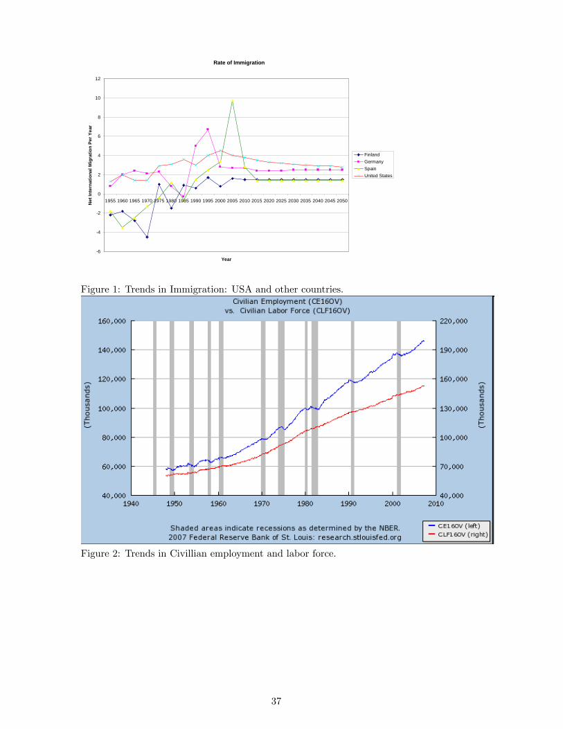
Rate of Immigration

6

4

2

0

2

4

6

8

10

12

1955 1960 1965 1970 1975 1980 1985 1990 1995 2000 2005 2010 2015 2020 2025 2030 2035 2040 2045 2050

Year

Net

Inte

rnat

iona

l Mig

ratio

n Pe

r Yea

r

FinlandGermanySpainUnited States

Figure 1: Trends in Immigration: USA and other countries.

Figure 2: Trends in Civillian employment and labor force.

37

Trends in Naturalization of Alliens in USA

0

200

400

600

800

1000

1200

1907

1910

1913

1916

1919

1922

1925

1928

1931

1934

1937

1940

1943

1946

1949

1952

1955

1958

1961

1964

1967

1970

1973

1976

1979

1982

1985

1988

1991

1994

1997

Fiscal Year

In T

hous

and

Figure 3: Trends in Naturalization of Aliens in USA. Source: United Nations

Figure 4: Trend in Part Time Jobs for the retirees(Cahill, Giandrea and Quinn(2005))

38

Figure 5: Trend in Transition to Part Time Jobs for the retirees(Cahill, Giandrea andQuinn(2005))

39

PAYGO FF Private AnnuityParameter De�nition Value Value Value� Skill Coe¢ cient for the Retiree 0:6 0:6 0:6� Discount Factor 0:96 0:958 0:96� Capital Depreciation rate 0:1 0:1 0:1� Intertemporal elasticity of substitution 0:25 0:25 0:25� Labor�s share in production 0:667 0:667 0:667! Retirement probability 0:997 0:997 0:997x Steady state growth rate of technology 0:01 0:01 0:01n Steady state growth rate of population 0:01 0:01 0:01

v Consumption share in the utility 0:5 0:5 0:5

� 1�vv 1:5 1:5 1:5

� Average social security tax 0:124 0:124 0:124

B Participation rate 0:2495 0:2495 0:2495Table 1: Exogenous Parameters of the Models

Impulse Response of Worker's Consumption to a Permanent Population Shock

0.045

0.04

0.035

0.03

0.025

0.02

0.015

0.01

0.005

0

0.005

0.01

1 8 15 22 29 36 43 50 57 64 71 78 85 92 99 106

113

120

127

134

141

148

155

162

169

176

183

190

197

Periods

Log

Dev

iatio

n fr

om S

tead

y St

ate

Private AnnuityPAYGO_DCFF_DBPAYGO_DBFF_DC

Figure 6: Impulse Response of worker�s consumption to a permanent population shock(LogDeviations from the steady state)

40

Scaled PrivateAnnuity PAYGO-DB FF-DB PAYGO-DC FF-DCVariables Initial Final Initial Final Initial Final Initial Final Initial FinalY 0:791 0:753 0:714 0:692 0:704 0:682 0:714 0:681 0:704 0:672Cw 0:434 0:417 0:369 0:363 0:367 0:361 0:369 0:358 0:367 0:357Cr 0:075 0:067 0:116 0:103 0:114 0:102 0:116 0:103 0:114 0:102L 0:460 0:456 0:437 0:437 0:434 0:435 0:437 0:433 0:434 0:431Lw 0:432 0:432 0:421 0:419 0:418 0:417 0:421 0:415 0:418 0:413Hw 6:502 5:955 3:726 3:564 3:638 3:478 3:726 3:439 3:638 3:357Hr 0:306 0:324 0:156 0:263 0:155 0:258 0:156 0:255 0:155 0:251K 2:391 2:122 1:953 1:790 1:889 1:733 1:953 1:742 1:889 1:687

Kw 1:994 1:811 1:7 1:213 1:643 1:167 1:70 1:101 1:643 1:054

Kr 0:397 0:291 0:254 0:160 0:245 0:154 0:254 0:140 0:245 0:134

� 0:166 0:137 0:130 0:089 0:130 0:089 0:130 0:080 0:130 0:080

W 1:148 1:102 1:091 1:056 1:081 1:047 1:091 1:050 1:081 1:041

R 1:012 1:021 1:024 1:032 1:027 1:035 1:024 1:034 1:027 1:036

� 0:051 0:054 0:068 0:070 0:069 0:072 0:068 0:071 0:069 0:072

" 0:107 0:111 0:126 0:130 0:128 0:132 0:126 0:130 0:128 0:132

0:209 0:191 0:209 0:191 0:209 0:191 0:209 0:191 0:209 0:191

Lr 0:016 0:037 0:010 0:024 0:010 0:024 0:010 0:023 0:010 0:024

TaxRate 0:124 0:114 0:124 0:114 0:124 0:124 0:124 0:124

SS Bene�t 0:0569 0:0503 0:0569 0:0499 0:0569 0:05 0:0564 0:0496Table 2: Comparison between Initial and Final steady state after a permanent Population shock

Variable PrivateAnnuity PAYGO-DB FF-DB PAYGO-DC FF-DCY �0:015 -0.014 -0.013 -0.017 -0.017Cw 0.004 0.003 0.003 0.005 0.005Cr 0.063 0.039 0.039 0.049 0.048AbsDi¤ 0.060 0.036 0.035 0.044 0.043L -0.017 -0.016 -0.015 -0.021 -0.02Lw -0.002 0.001 0.001 -0.002 -0.002Hw -0.039 -0.0019 -0.019 -0.034 -0.034Hr 0.1040 0.336 0.329 0.265 0.257K -0.016 -0.017 -0.017 -0.019 -0.019Kw -0.015 -0.04 -0.044 -0.047 -0.045Kr -0.044 -0.064 -0.067 -0.074 -0.071� -0.028 -0.047 -0.05 -0.055 -0.052W 0.002 0.002 0.002 0.004 0.004R -0.001 0.0 0.0 -0.001 -0.001� 0.036 0.033 0.033 0.038 0.038" 0.024 0.024 0.024 0.026 0.026 -0.10 -0.010 -0.010 -0.01 -0.010Lr -0.266 -0.010 -0.010 -0.01 -0.010Sw -0.071 -0.071 -0.034 -0.035Sr -6.349 -6.169 -2.925 -2.839Tax Rate -0.010 -0.018Bene�t Rate 0.008 -0.004Total Bene�t(TB) -0.008 -0.008 -0.006 -0.006Table 3: Immediate response of a permanent population shock under alternative social security

arrangements(Log-deviations from the steady state).

41

Social Security Systems Initial Steady State Final Steady StateV w V r V V w V r V

Private Annuity 0.026 0.013 0.024 0.027 0.012 0.025PAYGO-DC 0.033 0.024 0.031 0.034 0.022 0.032FF-DC 0.034 0.024 0.032 0.035 0.023 0.033PAYGO-DB 0.033 0.024 0.031 0.034 0.022 0.032FF-DB 0.034 0.024 0.032 0.035 0.023 0.033

Table 4: Welfare calculations before and after a permanent population shock(� = 0:124)

Scaled PrivateAnnuity PAYGO-DC FF-DB PAYGO-DB FF-DCVariables (Periods) (Periods) (Periods) (Periods) (Periods)Y 87 44 63 64 45

Cw 55 75 80 71 80

Cr 89 71 59 60 74

L 65 53 64 56 55

Lw 52 74 60 60 71

Hw 51 61 63 71 47

Hr 86 87 67 73 70

K 53 60 59 74 50

� 72 91 84 92 95

W 49 61 55 48 76R 33 52 41 34 24� 44 58 72 59 58" 38 37 45 43 43 73 73 73 73 73Lr 85 70 83 75 81

Table 5: Speed of convergence after a permanent population shock under alternative socialsecurity systems

Scaled PrivateAnnuity PAYGO-DB FF-DB PAYGO-DC FF-DCVariables (Periods) (Periods) (Periods) (Periods) (Periods)STD(Y ) 5.99 2.88 2.67 2.95 2.73STD(Cw) 4.91 2.36 2.21 2.44 2.28STD(Cr) 4.16 2.02 1.91 2.09 1.98STD(K) 2.51 1.33 1.29 1.37 1.32STD(W ) 2.24 1.24 1.20 1.26 1.23STD(R) 2.15 1.21 1.17 1.23 1.20STD(C

w

Cr ) 1.18 1.17 1.16 1.17 1.16STD(C

w

Y ) 0.82 0.82 0.83 0.83 0.84STD(C

r

Y ) 0.69 0.70 0.71 0.71 0.72STD(KY ) 0.42 0.46 0.48 0.46 0.78

Table 6: Comparison of Volatility under alternative social security systems(Standard deviationof the scaled variables)

42

Impulse Response of Retiree's Consumption to a Permanent Population Shock

0.15

0.1

0.05

0

0.05

0.1

1 10 19 28 37 46 55 64 73 82 91 100 109 118 127 136 145 154 163 172 181 190 199

Periods

Log

Dev

iatio

n fr

om S

tead

y St

ate


Figure 7: Impulse Response of retiree�s consumption to a permanent population shock(LogDeviations from the steady state)

Impulse Response of Capital to a Permanent Population Shock

0.14

0.12

0.1

0.08

0.06

0.04

0.02

01 10 19 28 37 46 55 64 73 82 91 100 109 118 127 136 145 154 163 172 181 190 199

Periods

Log

Dev

iatio

n fr

om S

tead

y St

ate


Figure 8: Impulse Response of capital to a permanent population shock(Log Deviations fromthe steady state)

43

Impulse Response of Output to a Permanent Population Shock

0.06

0.05

0.04

0.03

0.02

0.01

01 10 19 28 37 46 55 64 73 82 91 100 109 118 127 136 145 154 163 172 181 190 199

Periods

Log

Dev

iatio

n fr

om S

tead

y St

ate


Figure 9: Impulse Response of output to a permanent population shock(Log Deviations fromthe steady state)

Transition Dynamics of Worker's Consumption after a Permanent Population Shock

0

0.05

0.1

0.15

0.2

0.25

0.3

0.35

0.4

0.45

0.5

1 9 17 25 33 41 49 57 65 73 81 89 97 105 113 121 129 137 145 153 161 169 177 185 193

Period

Wor

ker's

Con

sum

ptio

n


Figure 10: Transitional dynamics of worker�s consumption to a permanent population shock(inlevels)

44

Transition Dynamics of Retiree's Consumption after a Permanent Population Shock

0

0.02

0.04

0.06

0.08

0.1

0.12

0.14

1 9 17 25 33 41 49 57 65 73 81 89 97 105 113 121 129 137 145 153 161 169 177 185 193

Period

Ret

iree

s C

onsu

mpt

ion


Figure 11: Transitional dynamics of retiree�s consumption to a permanent population shock(inlevels)

Transition Dynamics of Capital after a Permanent Population Shock

0

0.5

1

1.5

2

2.5

1 9 17 25 33 41 49 57 65 73 81 89 97 105 113 121 129 137 145 153 161 169 177 185 193

Period

K


Figure 12: Transitional dynamics of capital to a permanent population shock(in levels)

45

Transition Dynamics of Ouput after a Permanent Population Shock

0.6

0.62

0.64

0.66

0.68

0.7

0.72

0.74

0.76

0.78

0.8

1 9 17 25 33 41 49 57 65 73 81 89 97 105 113 121 129 137 145 153 161 169 177 185 193

Period

Y


Figure 13: Transitional dynamics of output to a permanent population shock(in levels)

Transition Dynamics of Wage after a Permanent Population Shock

0.98

1

1.02

1.04

1.06

1.08

1.1

1.12

1.14

1.16

1 9 17 25 33 41 49 57 65 73 81 89 97 105 113 121 129 137 145 153 161 169 177 185 193

Period

W


Figure 14: Transitional dynamics of wage to a permanent population shock(in levels)

46

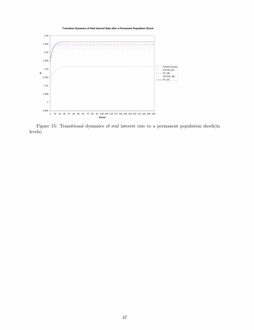
Transition Dynamics of Real Interest Rate after a Permanent Population Shock

0.995

1

1.005

1.01

1.015

1.02

1.025

1.03

1.035

1.04

1 10 19 28 37 46 55 64 73 82 91 100 109 118 127 136 145 154 163 172 181 190 199

Period

R


Figure 15: Transitional dynamics of real interest rate to a permanent population shock(inlevels)

47

Documents

Demographic Uncertainty and Welfare in a Life-cycle Model