DEMOGRAPHIC RESEARCH VOLUME 10, ARTICLE 2, … · of peer-reviewed research ... female cohorts confronted with an extreme unbalanced marriage market ... In his seminal article ‘European

Demographic Research a free, expedited, online journal of peer-reviewed research and commentary in the population sciences published by the Max Planck Institute for Demographic Research Konrad-Zuse Str. 1, D-18057 Rostock · GERMANY www.demographic-research.org

DEMOGRAPHIC RESEARCH VOLUME 10, ARTICLE 2, PAGES 27-60 PUBLISHED 26 FEBRUARY 2004 www.demographic-research.org/Volumes/Vol10/2/ DOI: 10.4054/DemRes.2004.10.2 Research Article

Marriage in Russia. A reconstruction

Sergei Scherbov

Harrie van Vianen

© 2004 Max-Planck-Gesellschaft.

Table of Contents

1 Introduction 28

2 Marriage in Russia: an analysis 312.1 Marriage in Russia: histories 322.2 Marriage in Russia: statistics 352.3 Marriage in Russia, multistate marital tables 432.3.1 Time spent in marital states 442.3.2 Number of transitions between marital states 462.3.3 Age at transition between marital states 492.3.4 Conditional probabilities 52

3 Conclusions 57

Notes 59

References 60

Demographic Research – Volume 10, Article 2

http://www.demographic-research.org 27

Research Article

Marriage in Russia:A reconstruction

Sergei Scherbov1

Harrie van Vianen2

Abstract

The micro census 1994 of the Russian Federation collected detailed marital histories forall respondents. This information made it possible to construct multistate marital tablesfor both male and female cohorts born since 1910 for the first time. Continuity andchange in marital patterns over a most turbulent of Russian history could be analyzed.Divorce rose monotonously from a quite low level for the cohort of 1910 to the highincidence that is characteristic for modern Russia. The typical Eastern Europeanmarriage pattern of early and almost universal marriage was remarkably stable. Themajor crisis, the Second World War, led to a postponement of marriage, but even in thefemale cohorts confronted with an extreme unbalanced marriage market the proportionnever married was remarkably low.

1 Corresponding Author. Vienna Institute of Demography, Austrian Academy of Sciences. Prinz

Eugen-Straße 8-10, A-1040 Vienna, Austria. Email: [email protected] Vienna Institute of Demography


28 http://www.demographic-research.org

1. Introduction

In his seminal article ‘European marriage patterns in perspective’ Hajnal distinguishedan Eastern European pattern that was completely different from the Western Europeanpattern. East from a line that stretched roughly from St. Petersburg to Trieste marriagewas very frequent and early. In contrast to the West where the marriage patternunderwent profound changes in Russia early and almost universal marriage haveremained typical. According to the latest 1994 micro census only 6 percent of men and5 percent of women were never married at age 50. The proportion of people gettingmarried at very young ages even has been growing recently. In the 1917 cohort 29percent of women married before age 20 and 24 percent of men married before age 23.In the cohort 1960 these proportions were 32 percent and 44 percent respectively. Thispersistence of two of the characteristics of marriage should not make one lose sight ofthe fact that in Russia as elsewhere marriage is a complex phenomenon in a constantstate of flux (Avdeev and Monnier, 1999, 635).

In the twentieth century Russian society made a major transition. At the beginningof the century Russia was still predominantly traditional and rural, but during thecentury it shifted to an industrialized, urbanized modern highly educated society. Thistransition did not develop continuously, but was accompanied by severe shocks thatcompletely upset the life of the citizen and had profound effects upon the primaryinstitution of the family. Especially the huge male deficits in the cohorts that were mostaffected by the Second World War led to substantial adjustments in the patterns ofmarriage, divorce, widowhood and remarriage. The very small sizes of the cohorts bornduring the war years and the preference for brides that are at average about two yearsyounger than their grooms should have had sizable effects upon nuptiality in the 1960’swhen these cohorts entered the marriage market. Moreover the state tried to intervenedecisively into the process of family formation and procreation (for an overview seeAvdeev and Monnier 1999, annex 1).

In their recent analysis of various aspects of marriage in Russia, Avdeev andMonnier had to limit themselves essentially to the period since around 1960. After the1926 census the population registration system in the former Soviet Union collapsedand it is only since 1959 that reliable population figures from censuses and registrationare available. Part of the demographic history of Russia in the intervening period wasreconstructed recently, using archive materials and demographic estimation (Andreev,Darsky and Kharkova, 1998). Detailed information from official statistics is unavailablebut thanks to the possibilities of a retrospective investigation of data collected duringthe five-percent micro census of 1994 at least some questions can be answered.

In the 1994 micro census some 5 percent, 7.35 million persons, of the totalpopulation of the Russian Federation was interviewed. The Statistical Office of the



Russian Federation published the principal results in aggregate tabular form in 8volumes (Goskomstat1995). Volkov (1999) discussed the representativeness of themicro census. The detailed nature of the individual data permits for a reconstruction ofpart of the life course of separate subpopulations and for the calculation of a number ofdemographic statistics from the past. In two earlier articles we analyzed cohort fertilityand female nuptiality (Scherbov and Van Vianen 1999, 2001). A third articlereconstructed period fertility since 1930, using a modeling approach (Scherbov and VanVianen, 2002). In this paper both male and female nuptiality will be analyzed morecompletely.

With respect to marriage the micro census included a number of questions onmarital careers: date of first marriage, date and cause of first marriage termination(divorce, death of spouse), date of second marriage, and total number of marriages. Thisfeature of knowing the date of certain events on an individual basis allows for theconstruction of multistate marital tables (Willekens 1987, Darsky and Scherbov 1995).The micro census contains all necessary information on first marriages. For men andwomen widowed or divorced from first marriage we know the date of dissolution andthe date of an eventual remarriage. Finally we know the current status, though not thedate or cause of subsequent events, but using acceptable hypotheses we can calculatetransition probabilities and construct the multistate marital tables. The methodologicalapproach is essentially the same as set out in the paper by Darsky and Scherbov (1995,35-38), except that in our cohort study we do not have to make the additionalassumption of a stationary population, which is necessary in order to apply period ratesto a hypothetical cohort.

A multistate marital table depicts the marital career of a birth cohort from age 16until some final age, which in our study we fix at age 50: the end of the reproductiveperiod for women. It states the probabilities of being never married, married, widowedor divorced at any age for a person being single at age 16. The main advantage of thesetables over conventional marital tables is that they consider not only first marriages,divorces and loss of spouses by death, but also remarriages of widowed and divorcedmen and women. Using the tables we can evaluate conditional probabilities for a personof being in a certain marital state at a certain age given his marital state at an earlierage. We can also decompose the life span between 16 and 50 by the number of yearsspent in various states. In this way we get a complete picture of marital state changesduring the life of a cohort. The table describes the ‘pure’ marital process, i.e. the tableexcludes the exit processes of death and out migration. However, death of a spouse isexplicitly taken into account and effects the widowhood process. Because the data usedin constructing the tables are retrospective a selection bias will be present, especially forthe oldest cohorts: we can only calculate the various transition probabilities from the



marital histories of those members of the original birth cohort that were still alive at thedate of census taking.

In our analysis we study the marital histories of successive birth cohorts. In anearlier article we underlined the importance of taking a cohort perspective whenstudying demographic change. Whereas period measures are shaped by conjuncturaleffects and may behave irregularly because of many factors affecting marital decisions,cohort measures more truly reflect underlying lifetime motivations (Scherbov and VanVianen 1999). Moreover our data are most applicable for a cohort approach. They ofcourse allow for the calculation of certain age specific period indicators, butinformation on the size and the age distribution of the population is missing for most ofthe period between 1926 and 1959 and therefore many period indicators on thepopulation level are unobtainable. We can for instance calculate age specific firstmarriage rates in a certain year, but in order to obtain the total number of marriages orthe crude marriage rate in that year we need the absolute age composition for that year.

Another aspect of our retrospective data set is that all people were born after acertain year. In 1994 there are only few survivors of the oldest generations and theirinformation will certainly not be representative for the cohort experience. In practicethis means that for women we can go back until 1900, there being more than 1000respondents from that year onwards, a number that goes up to 16,000 respondents bornin 1910: all succeeding cohorts are larger. Starting from 1900 this implies that forinstance for 1935 we only have information for women up to 35 years of age in thatyear. Consequently our information on a period measure up to age 50 is censored beforethe year 1950; only from that year onward our period measures would be complete.

Due to the imbalance of the Russian age distribution we only have 180 males bornin 1900 in our sample and 4000 born in 1910. Only starting from the cohort of 1922 wehave more than 10,000 male respondents in each succeeding cohort. We made thepragmatic decision to limit our study of both male and female nuptiality to cohorts bornsince 1910.

In the 1994 micro census a distinction was made between married and living in aconsensual union and between divorced and separated. Since for most of the cohorts towhich our analysis applies cohabitation and separation was infrequent we do not retainthese distinctions but combine married and living in consensual union and divorced andseparated. An additional problem in this respect is that family and marriage legislaturechanged several times between 1917 and 1967. For instance in 1944 recognition ofcohabitation was withdrawn which triggered off a wave of marriages ‘of regularization’(Avdeeev and Monnier 1999, 637). Moreover all data in the micro census are ‘selfreported’ and respondents may have given a ‘socially correct’ answer for their maritalstate.



In the next section we will first show multistate marital tables for some selectedcohorts. Multistate marital tables for males are quite unique; we could not find otherexamples. To a lesser extent this applies to male nuptiality as a whole. In the thirdsection a number of indicators, derived from the multistate tables will be presented forboth sexes and for all cohorts for which they can be calculated. In the last section wewill draw some conclusions about the changes in Russian nuptiality that can be derivedfrom our analysis.

2. Marriage in Russia: an analysis

Multistate marital tables can be constructed for all cohorts present in the micro census.But, as explained before we only started from 1910, because the number of survivingmales in older cohorts is very low. All cohorts born since 1944 were not yet aged 50 orover on 14 February 1994 and therefore they are censored by the date of the microcensus. We limit our analysis to cohorts born before 1961. Those born in 1960 reachedthe age of 33 before the date of the micro census and because Russians marry young amarital table censored at age 33 can, when interpreted cautiously, still give usefulinformation. When applicable, results for cohorts up to 1970 will be shown



2.1. Marriage in Russia: histories

Figure 1a

Figure 1b



Figure 1c

Figure 1d

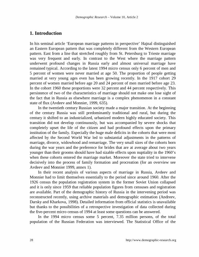
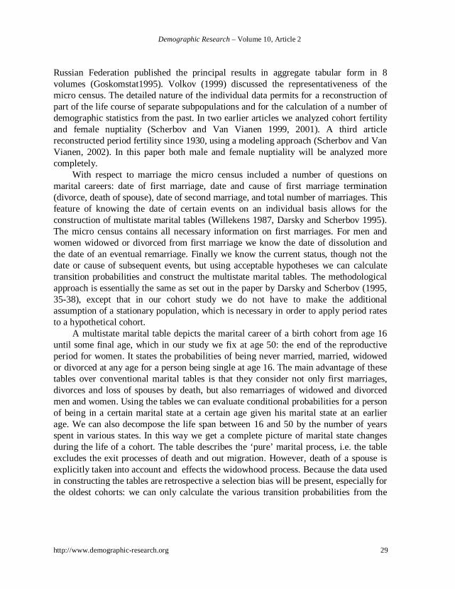
Figure 1: Multistate marital tables for some selected cohorts



In figure 1a to 1d we present multistate marital tables for some selected cohorts. Inorder to get some insight into the different histories of men and women we willcompare the history of a male cohort with the experience of the female cohort that istwo years younger. The difference of mean age at marriage is around 2 years for mostcohorts, but of course men from a certain cohort can marry women from all cohorts onthe marriage market. First we will discuss figure 1a: the male cohort of 1918. At age 23,before the German invasion and the start of the Great Patriotic War nearly 20 percent ofmen were married. Between age 23 and 27, during the war years, the proportionmarried rose only slowly, but after 1945 it increased very rapidly till 80 percent at age31. The proportions widowed and divorced were always very low in this cohort andultimately only around 4 percent of males was never married at age 50.

Figure 1b: the female cohort of 1920 tells a quite different story. The proportionmarried rises very rapidly, until at age 21 around 35 percent of women is married.During the war new marriages only compensated for early widowhood and theproportion married in this cohort never is above 70 percent. At age 50 more than 10percent is never married but 20 percent is widowed, indicating that most women whowere widowed at a young age did not remarry.

In figure 1c the male cohort 1948 is shown. It is censored at age 46. At age 23more than 40 percent is married. There is no delay and at age 31 more than 80 percentis married, a proportion growing slowly afterwards. Only 7 percent is never married atage 46. Widowhood does not amount to anything for this generation, but the proportiondivorced at age 46 is higher than the proportion never married.

The females of 1950 (figure 1d) have a different history. At age 21 around 40percent is married, the same proportion as in the 1948 male cohort, a proportion risingto around 80 percent at age 29. But widowhood and to a larger extent divorce play arole and the proportion married is constant after age 29 till the age of censoring. At age44 around 5 percent is never married, about the same proportion is widowed. The majorfactor of this difference with the male cohort of 1948 is of course the high differentialbetween female and male mortality, another characteristic of Russian demography.Compared with the male experience a substantial higher proportion of women isdivorced.



2.2. Marriage in Russia: statistics

Figure 2: Proportion women and men never married at age 50

In figure 2 we present the proportion women and men never married at age 50 or by theage at censoring by census date for all cohorts born between 1910 and 1960. Note thatonly the cohorts born before 1944 reached this final age of 50 before the date of themicro census. For women the proportion never married increases from around 6 percentin the oldest cohorts to more than 10 percent in the cohorts most heavily affected by theSecond World War. It monotonously declines to around 4 percent in the (very small)cohorts born during the war. Afterwards it slowly increases again, but remains very lowuntil the last cohorts, a first indication of a change in marriage pattern with a decline inthe rate of first marriages.

For males the pattern is different. Up to the cohort of 1940 it is always under 5percent, between 1936 until around 1950 it is about the same as for women butafterwards it increases more steeply. For the youngest cohorts the increase is partly dueto censoring.



Figure 3: Mean age at first marriage

Figure 3 shows the distribution of the mean age at first marriage for both females andmales. For women it goes up from around 22 years in the oldest generations to amaximum of 24.5 years for the generations born in 1922 and 1923. Afterwards it fallsoff almost linearly. Again this feature is genuine. Due to the very young age at firstmarriage censoring does not play any role. When combining this result with theforegoing figure we see that there is a decline in the mean age at marriage simultaneouswith a decline in the proportions marrying (Avdeeev and Monnier 1999, 637-638)

For males the developments are not the same. In the older cohorts the difference inage at first marriage is around 4 years, whereas in the younger generations it is around 2years. In the oldest cohorts these differences in age at marriage may reflect imbalancescaused by the period of the Civil War. The cohorts born between 1920 and 1925 weremost heavily afflicted by the Second World War, which not only caused a majorimbalance in the sex ratio at marriageable ages but marriage was nearly impossibleduring the war with most marriageable males in the armed forces, a situation lengthenedby the problems of demobilization and reconstruction after the war. In the youngergenerations we also observe the decline of the age at first marriage. An interestingeffect is the increase of the age at first marriage for the male generations born around1940. This is an indication of a squeeze in the marriage market when young men of thequite large birth cohorts of around 1940 with a preference for brides about 2 yearsyounger entered the marriage market and were confronted with the extremely smallfemale generations of 1943 and 1944. A similar effect for the larger female generations



of 1945-1946 when confronted with the small male cohorts born in 1943.and 1945 doesnot appear. This asymmetry has to do with the different pattern of age at marriage. Forfemales it is very peaked around the modal age of 20, whereas for males the spreadaround 23 years is much larger, which implies that for a female there would be moreeligible candidates on the marriage market.

Figure 4: Lexis surface of proportions of women first marrying by year of birth, perthousand

A much more instructive picture emerges if we do not confine our study to a centralmeasure like mean age at marriage but include the distribution of age at first marriage.In figure 4 we present a Lexis surface of proportions of women first marrying by yearof birth and single year of age, because these are just rates we present them up to the



cohort 1970. The concentration of marriages around the modal age is distorted by theevents of around 1932 and 1933, the Famine. A more normal pattern appears afterwardsbut another, deeper, trough is caused by the Second World War. In the female birthscohorts most heavily affected, those born in 1916-1922, the distribution of age at firstmarriage becomes bimodal. The shortfall of marriages is made up after the war, but theconcentration of marriages, although at a somewhat higher modal age reappears only inthe generations born after 1934. In the following generations there is a slight decreasein the age and the distribution becomes more peaked around the modal age. Althoughthe official age at which a woman can marry is 18 years, an appreciable number ofmarriages before this age are reported.

Figure 5: Lexis surface of proportions of men first marrying by year of birth, perthousand



The same distribution for males is presented in figure 5. Males marry at a higherage and the age at marriage has a wider range. In particular for the oldest cohorts thespread of age at marriage for males is much larger as compared with females, whichexplains the larger difference of mean age at marriage from figure 2. For males theeffects of the war are even more outspoken than for females. For all generations from1910 until1922 the distribution is bimodal and the concentration of marriagesimmediately after the war for the generations 1918-1922 is evident. These generationsreally had to postpone marriage and were small when entering a marriage market with alarge imbalanced sex ratio.

Although the distribution of age at marriage was severely distorted by the societalupheavals of famine and war the proportion of women never married shows onlyrelatively minor effects. This is the more remarkable because the female cohorts bornbetween 1923 and 1926 were already larger than the corresponding male cohorts of1919-1922 due to the effects of the Civil War. The Second World War made theseimbalances even worse. These findings are consistent with an earlier analysis of theeffects of the First World War on nuptiality of French women by Louis Henry (1966).The radically depleted size of certain male cohorts was compensated for by a shift inmarital preferences, resulting in only modest changes in the proportion women nevermarrying. The long-term trend shows that the institution of marriage retained most ofits traditional features during this period.



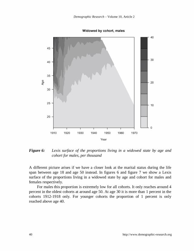
Figure 6: Lexis surface of the proportions living in a widowed state by age andcohort for males, per thousand

A different picture arises if we have a closer look at the marital status during the lifespan between age 18 and age 50 instead. In figures 6 and figure 7 we show a Lexissurface of the proportions living in a widowed state by age and cohort for males andfemales respectively.

For males this proportion is extremely low for all cohorts. It only reaches around 4percent in the oldest cohorts at around age 50. At age 30 it is more than 1 percent in thecohorts 1912-1918 only. For younger cohorts the proportion of 1 percent is onlyreached above age 40.



Figure 7: Lexis surface of the proportions living in a widowed state by age andcohort for females, per thousand

For women the situation is much more dramatic. First note the difference in scale infigure 7. In the oldest cohorts widowhood reaches proportions above 40 percent. In thecohort 1921 more than 5 percent of women are already widowed at age 22. In theyounger cohorts, born since 1927, it is only above age 40 that the proportion widowedis more than 5 percent. These high proportions of widowed females when comparedwith widowed males not only reflect the immediate consequences of male mortalityduring the war. Other factors are the difference in age at marriage, the ‘normal’mortality, which for males is substantially higher and the imbalance of the sex ratio,which made remarriage much easier for a widowed male.



Figure 8: Lexis surface of the proportions living in a divorced state by age andcohort for males, per thousand



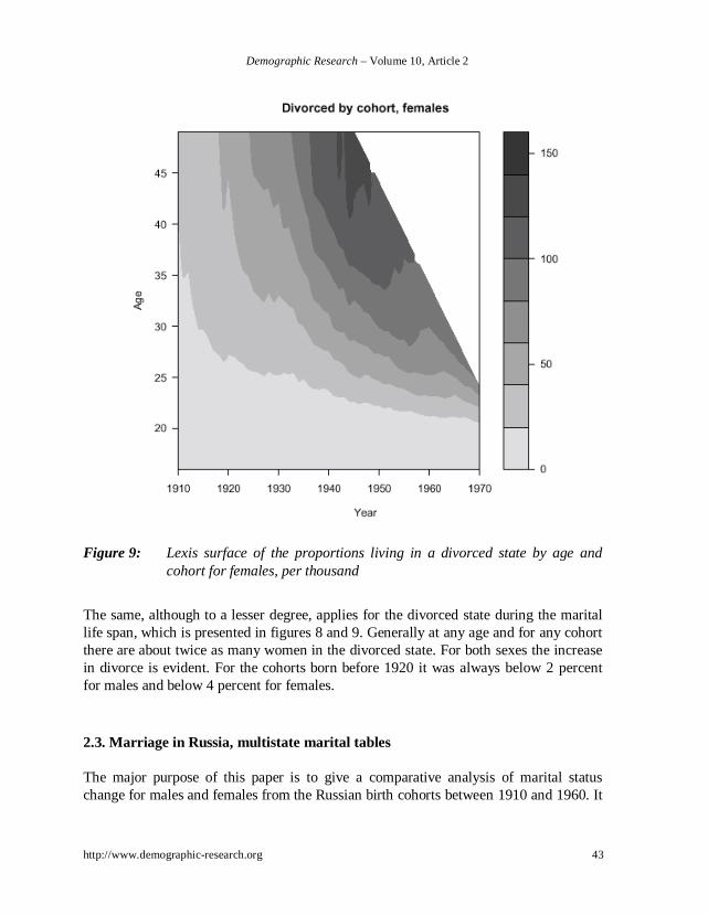
Figure 9: Lexis surface of the proportions living in a divorced state by age andcohort for females, per thousand

The same, although to a lesser degree, applies for the divorced state during the maritallife span, which is presented in figures 8 and 9. Generally at any age and for any cohortthere are about twice as many women in the divorced state. For both sexes the increasein divorce is evident. For the cohorts born before 1920 it was always below 2 percentfor males and below 4 percent for females.

2.3. Marriage in Russia, multistate marital tables

The major purpose of this paper is to give a comparative analysis of marital statuschange for males and females from the Russian birth cohorts between 1910 and 1960. It



is impossible to present the detailed transition probabilities of all the multistate maritaltables over such a long period and therefore we limit ourselves to the presentation of anumber of indicators from our marital tables for both sexes and for all cohorts. Inestimating marital tables we could use data on date of first marriage, date and cause ofend of first marriage and date of second marriage for each individual in the microcensus. So we could directly estimate the age specific probabilities of first marriage,dissolution of first marriage by divorce, dissolution of first marriage by widowhood,probabilities of second marriage from divorce and probabilities of second marriagefrom widowhood. Because there are no detailed data on dissolution of remarriages theywere modeled as follows: a person who is divorced or widowed can remarry withremarriage probabilities estimated from our data. When remarrying he reenters the stateof married and the probabilities of divorce and widowhood are the same as thoseestimated from the data on first marriages (Darsky and Scherbov 1995, 36,37).

In our cohort analysis we have only complete information from those cohorts thatwere aged 50 or over at the date of the micro census: the cohorts born before 1944. Alllater cohorts are censored. The latest cohort in our analysis, the cohort of 1960 was 33years in 1994. In order to construct multistate tables for these censored cohorts wecould impute the last transition probabilities that were observed for the missingprobabilities. The transition probabilities at age 49 from the 1943 cohort, those at age48 from the 1944 cohort etc. This procedure would imply that the completed tables area mixture of a cohort table up to the age at the micro census and a period table forhigher ages. However, transition probabilities at a certain age are dependent upon theforegoing marital history of the cohort and this implies that an uncontrollable bias isintroduced by a marital history after the censored age that is a mixture of the maritalhistories of older cohorts, but that does not describe the history of any ‘real’ cohort.Ultimately, for the cohorts born after 1977 we would end up with a pure period maritaltable.

We adopted another approach for completing the life table. After the censored ageno transition is possible and the distribution over the marital states (never married,married, divorced and widowed) is stationary. In this procedure only observedtransitions are taken into account, but a systematic bias of exclusion of transitions atages after censoring is introduced. This bias will be increase monotonically over thecensored cohorts.

2.3.1. Time spent in marital states



Table 1: Number of years spent in different marital states during the reproductiveperiod (16-50 years) by sex and year of birth (1910-1960), Russia.

Females MalesYear Never Married Married Divorced Widowed Year Never Married Married Divorced Widowed

1910 9.07 18.16 0.46 6.30 1910 12.43 20.64 0.35 0.581911 9.12 17.71 0.55 6.62 1911 13.00 20.16 0.36 0.471912 9.09 17.94 0.55 6.42 1912 12.15 20.99 0.36 0.501913 9.30 17.78 0.60 6.32 1913 12.18 20.93 0.39 0.501914 9.55 17.53 0.69 6.23 1914 12.25 20.91 0.41 0.421915 9.41 17.81 0.69 6.09 1915 12.60 20.60 0.41 0.391916 9.71 17.72 0.71 5.85 1916 12.80 20.44 0.38 0.381917 9.81 17.95 0.84 5.40 1917 12.62 20.62 0.33 0.431918 10.10 18.16 0.85 4.89 1918 12.35 20.93 0.39 0.331919 10.57 18.08 0.92 4.43 1919 12.19 21.17 0.35 0.291920 11.14 18.29 0.86 3.72 1920 12.13 21.21 0.37 0.291921 11.40 18.61 0.93 3.07 1921 11.59 21.79 0.36 0.271922 11.60 18.94 1.01 2.45 1922 11.26 22.04 0.43 0.271923 11.52 19.36 1.07 2.05 1923 10.89 22.50 0.38 0.231924 11.34 19.79 1.10 1.77 1924 10.62 22.65 0.49 0.241925 10.95 20.29 1.19 1.57 1925 10.74 22.58 0.45 0.231926 10.62 20.67 1.23 1.48 1926 10.65 22.64 0.50 0.221927 10.29 21.00 1.26 1.44 1927 10.27 22.97 0.53 0.231928 10.07 21.31 1.23 1.40 1928 10.32 22.92 0.56 0.201929 9.91 21.51 1.29 1.30 1929 10.32 22.88 0.60 0.201930 9.78 21.64 1.28 1.31 1930 10.43 22.75 0.60 0.211931 9.58 21.80 1.36 1.26 1931 10.49 22.63 0.68 0.191932 9.36 22.03 1.37 1.24 1932 10.28 22.80 0.72 0.191933 9.30 21.96 1.45 1.30 1933 10.29 22.70 0.80 0.211934 8.90 22.30 1.58 1.23 1934 10.27 22.66 0.88 0.201935 8.85 22.26 1.65 1.24 1935 10.22 22.63 0.96 0.191936 8.59 22.47 1.74 1.19 1936 10.20 22.53 1.08 0.191937 8.54 22.33 1.98 1.15 1937 10.43 22.23 1.14 0.191938 8.36 22.50 2.03 1.12 1938 10.41 22.18 1.21 0.201939 8.32 22.50 2.07 1.10 1939 10.58 21.97 1.26 0.191940 8.19 22.56 2.16 1.08 1940 10.78 21.65 1.38 0.191941 8.07 22.60 2.26 1.07 1941 10.76 21.71 1.34 0.191942 8.08 22.52 2.36 1.04 1942 10.82 21.63 1.37 0.181943 8.07 22.59 2.36 0.98 1943 10.73 21.57 1.53 0.171944 8.10 22.41 2.57 0.92 1944 10.68 21.55 1.59 0.181945 8.12 22.46 2.52 0.90 1945 10.55 21.70 1.57 0.181946 8.05 22.51 2.53 0.91 1946 10.17 22.14 1.54 0.151947 8.04 22.58 2.54 0.84 1947 9.99 22.31 1.56 0.151948 8.03 22.61 2.58 0.79 1948 9.87 22.44 1.56 0.141949 7.85 22.77 2.59 0.79 1949 9.84 22.42 1.60 0.151950 7.82 22.88 2.58 0.72 1950 10.07 22.22 1.59 0.121951 7.78 22.93 2.61 0.68 1951 9.84 22.41 1.64 0.111952 7.73 23.03 2.58 0.66 1952 9.92 22.33 1.64 0.111953 7.65 23.20 2.56 0.60 1953 10.01 22.23 1.65 0.111954 7.70 23.08 2.62 0.60 1954 10.15 22.12 1.63 0.101955 7.60 23.34 2.52 0.54 1955 10.17 22.14 1.59 0.101956 7.60 23.35 2.54 0.51 1956 10.32 22.03 1.57 0.081957 7.67 23.39 2.48 0.46 1957 10.41 21.98 1.54 0.071958 7.73 23.43 2.42 0.42 1958 10.54 21.85 1.54 0.071959 7.73 23.42 2.45 0.40 1959 10.71 21.77 1.44 0.071960 7.93 23.29 2.42 0.36 1960 11.14 21.43 1.38 0.05



Only by using the multistate approach it is possible to describe the marital careerof a cohort in detail. Table 1 describes how the period of marital life between the ages16 and 50 is distributed among different marital statuses, conditional that a personsurvives until age 50. Note that the marital state can be entered more than once byremarriage.

For women the number of years spent in the never married state goes up from 9.1in the oldest cohorts to 11.6 years in the cohort around 1922 that had to postponemarriage or did not marry at all due to the Second World War. Afterwards it decreasesmonotonically until around 1955. Note that the decline after 1944 is underestimated inour figures, because women who were not married at the age of censoring stayed in thestate of never married. In the oldest cohorts women spent on average more than 6 yearsof their reproductive period being widowed. This goes down to less than 1 year in the1943 cohort. Afterwards it declines further but more and more of this decline is due tocensoring bias. The number of years spent in a divorced state increases steadily, exceptfor the (biased) youngest generations.

For men differences between the oldest cohorts may be due to the small cohortsizes before 1922. The number of years in the never married state is always higher thanfor the corresponding female cohorts except for the generations around 1922. Themonotonous decline after the war generations that we noted for females is not observedfor males. Note the slight increase for the generations 1939-1942, which contrasts withthe decrease in the female generations 1940-1943. Years spent in the widowed state arenegligible when compared with women and the years spent in a divorced state aresystematically less than for women of adjacent generations. Typically men and womenof all cohorts spent about the same number of years in the married state: men marrylater, but men that are divorced or widowed more often or more quickly remarried.Only in the oldest generations this balancing mechanism did not work due to the largenumber of females that could not marry or that were widowed during the war and thedistorted sex ratio on their marriage market.

2.3.2. Number of transitions between marital states

Table 2: Number of transitions between different marital states during thereproductive period (16-50 years) by sex and year of birth (1910-1960),Russia.



FemalesAll First Remarried after Number of times

Year marriages marriages Divorced Widowed Divorced Widowed1910 0.99 0.91 0.02 0.05 0.04 0.451911 0.99 0.91 0.02 0.06 0.05 0.451912 1.00 0.91 0.02 0.07 0.05 0.431913 1.00 0.91 0.02 0.07 0.05 0.421914 1.00 0.90 0.02 0.08 0.06 0.401915 1.01 0.91 0.02 0.08 0.06 0.391916 1.02 0.90 0.03 0.09 0.06 0.381917 1.02 0.90 0.03 0.09 0.07 0.361918 1.02 0.89 0.03 0.10 0.07 0.331919 1.01 0.89 0.03 0.09 0.07 0.311920 1.00 0.89 0.03 0.08 0.07 0.271921 0.99 0.89 0.03 0.07 0.08 0.241922 0.98 0.89 0.03 0.05 0.09 0.211923 0.97 0.90 0.04 0.04 0.09 0.191924 0.98 0.90 0.04 0.03 0.10 0.181925 0.98 0.91 0.04 0.03 0.11 0.161926 0.99 0.92 0.05 0.03 0.11 0.161927 1.00 0.92 0.05 0.03 0.12 0.161928 1.00 0.93 0.05 0.03 0.12 0.151929 1.01 0.93 0.05 0.03 0.12 0.151930 1.01 0.94 0.05 0.03 0.13 0.151931 1.02 0.94 0.05 0.03 0.13 0.151932 1.03 0.94 0.06 0.03 0.14 0.151933 1.03 0.94 0.06 0.03 0.14 0.151934 1.05 0.95 0.07 0.03 0.16 0.151935 1.06 0.95 0.07 0.03 0.17 0.151936 1.07 0.95 0.08 0.03 0.18 0.151937 1.07 0.95 0.09 0.03 0.20 0.141938 1.09 0.96 0.09 0.04 0.21 0.141939 1.09 0.95 0.10 0.04 0.21 0.131940 1.10 0.96 0.10 0.04 0.22 0.131941 1.10 0.96 0.11 0.04 0.23 0.131942 1.10 0.95 0.11 0.04 0.23 0.131943 1.11 0.95 0.12 0.04 0.24 0.131944 1.12 0.95 0.13 0.04 0.26 0.121945 1.11 0.95 0.13 0.03 0.25 0.111946 1.11 0.95 0.13 0.03 0.25 0.101947 1.11 0.95 0.13 0.03 0.25 0.091948 1.10 0.95 0.13 0.03 0.25 0.081949 1.11 0.95 0.13 0.03 0.25 0.081950 1.11 0.95 0.13 0.03 0.25 0.071951 1.10 0.95 0.13 0.02 0.25 0.071952 1.10 0.95 0.13 0.03 0.24 0.061953 1.10 0.95 0.13 0.02 0.24 0.051954 1.10 0.94 0.13 0.02 0.24 0.051955 1.10 0.94 0.13 0.02 0.24 0.051956 1.09 0.94 0.13 0.02 0.23 0.041957 1.08 0.94 0.13 0.02 0.23 0.041958 1.07 0.93 0.12 0.02 0.22 0.031959 1.06 0.93 0.12 0.01 0.22 0.031960 1.04 0.92 0.11 0.01 0.21 0.03



Table 2 (continued)

MalesAll First Remarried after Number of times

Year marriages marriages Divorced Widowed Divorced Widowed1910 1.01 0.93 0.04 0.04 0.05 0.081911 0.99 0.90 0.04 0.04 0.05 0.071912 1.03 0.95 0.04 0.04 0.06 0.071913 1.04 0.95 0.05 0.04 0.06 0.071914 1.04 0.96 0.05 0.03 0.07 0.061915 1.03 0.95 0.05 0.03 0.07 0.051916 1.03 0.95 0.05 0.03 0.07 0.051917 1.03 0.96 0.04 0.03 0.06 0.051918 1.04 0.96 0.05 0.03 0.07 0.051919 1.03 0.96 0.05 0.02 0.06 0.041920 1.02 0.96 0.04 0.02 0.06 0.041921 1.04 0.97 0.05 0.02 0.07 0.041922 1.04 0.96 0.05 0.02 0.07 0.041923 1.03 0.97 0.05 0.02 0.07 0.041924 1.04 0.97 0.06 0.02 0.08 0.041925 1.04 0.97 0.05 0.02 0.08 0.041926 1.04 0.97 0.06 0.02 0.08 0.041927 1.05 0.97 0.06 0.02 0.09 0.041928 1.05 0.97 0.06 0.02 0.09 0.041929 1.05 0.97 0.06 0.02 0.10 0.041930 1.04 0.97 0.06 0.02 0.10 0.041931 1.05 0.96 0.07 0.02 0.11 0.041932 1.05 0.96 0.07 0.02 0.11 0.041933 1.05 0.96 0.08 0.01 0.12 0.041934 1.06 0.96 0.08 0.02 0.13 0.041935 1.06 0.96 0.09 0.02 0.14 0.041936 1.07 0.96 0.09 0.02 0.15 0.041937 1.07 0.96 0.10 0.02 0.16 0.031938 1.08 0.96 0.11 0.01 0.17 0.031939 1.08 0.95 0.11 0.02 0.18 0.041940 1.08 0.95 0.12 0.01 0.19 0.031941 1.09 0.95 0.12 0.01 0.19 0.031942 1.09 0.95 0.13 0.01 0.19 0.031943 1.09 0.95 0.13 0.01 0.21 0.031944 1.10 0.95 0.14 0.01 0.21 0.031945 1.09 0.94 0.14 0.01 0.21 0.031946 1.09 0.95 0.13 0.01 0.20 0.021947 1.09 0.95 0.13 0.01 0.20 0.021948 1.08 0.94 0.13 0.01 0.20 0.021949 1.07 0.94 0.13 0.01 0.20 0.021950 1.06 0.93 0.13 0.01 0.19 0.021951 1.06 0.93 0.12 0.01 0.19 0.011952 1.06 0.93 0.12 0.01 0.19 0.011953 1.04 0.92 0.12 0.01 0.19 0.011954 1.03 0.91 0.11 0.00 0.18 0.011955 1.03 0.91 0.11 0.01 0.18 0.011956 1.02 0.90 0.11 0.00 0.17 0.011957 1.01 0.90 0.11 0.00 0.17 0.011958 0.99 0.89 0.10 0.00 0.16 0.011959 0.98 0.88 0.09 0.00 0.15 0.011960 0.95 0.87 0.08 0.00 0.14 0.01



Note that the number of marriages can be larger than one because of remarriagesfrom divorced or widowed. The way our tables are completed for the censored cohortsguarantees that the number of events in the table is the same as the observed number ofevents. The tables depict the average number of events per person in a cohort, but anindividual person may experience a certain event more than once.

Around 90 percent of women in the oldest cohorts married for the first time, afigure that does not change appreciably for the war cohorts around 1922. After 1926 itgoes up to around 95 percent and remains at that high level (except for the youngestgenerations, but here the number of events is underestimated due to censoring). In theoldest cohorts more than 40 percent experience the event of becoming widowed (itwould be more precise to say that 100 women experienced the event of becomingwidowed 40 times, because a woman can experience an event more than once betweenage 16 and age 50), only a fraction remarriages and most women remain widowed.Combining table 1 and 2 we can get an impression of the impact of the war on women’slives. In the 1914 cohort a woman was widowed on average 0.40 times and, accordingto table 1, every woman in this generation lived on average for 6.2 years in thewidowed state, so that the event of becoming widowed implied on average 15.5 years inthe widowed state. The average number of divorces per woman goes up from .04 in1910 to 0.24 in 1943; afterwards remains at that level. In the youngest generations weonly have the number of times divorced up to the age at censoring and the lifetimefigure certainly will be higher.

The number of first marriages for males is even higher than for females. Only inthe youngest cohorts there is a decline but that may be accounted for by censoring dueto the higher age at marriage of males. The number of times males are widowed isalways very low. The number of times divorced is systematically lower for males thanfor females, reflecting the difference in age at marriage, which may lead to more maledivorces above age 50 or age at censoring. This effect is particularly clear when wecompare the youngest cohorts. Moreover more male divorcees remarry, whichcorresponds with the finding in table 1 that males spent fewer years in the divorcedstate than females.

2.3.3. Age at transition between marital states

Table 3: Mean age at transitions between different marital states during thereproductive period (16-50 years) by sex and year of birth (1910-1960),Russia.



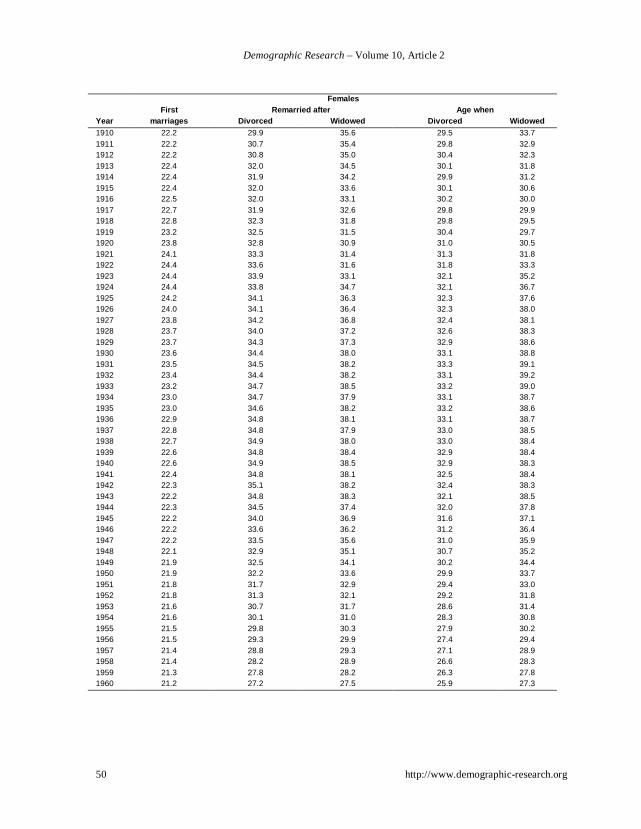
FemalesFirst Remarried after Age when

Year marriages Divorced Widowed Divorced Widowed1910 22.2 29.9 35.6 29.5 33.71911 22.2 30.7 35.4 29.8 32.91912 22.2 30.8 35.0 30.4 32.31913 22.4 32.0 34.5 30.1 31.81914 22.4 31.9 34.2 29.9 31.21915 22.4 32.0 33.6 30.1 30.61916 22.5 32.0 33.1 30.2 30.01917 22.7 31.9 32.6 29.8 29.91918 22.8 32.3 31.8 29.8 29.51919 23.2 32.5 31.5 30.4 29.71920 23.8 32.8 30.9 31.0 30.51921 24.1 33.3 31.4 31.3 31.81922 24.4 33.6 31.6 31.8 33.31923 24.4 33.9 33.1 32.1 35.21924 24.4 33.8 34.7 32.1 36.71925 24.2 34.1 36.3 32.3 37.61926 24.0 34.1 36.4 32.3 38.01927 23.8 34.2 36.8 32.4 38.11928 23.7 34.0 37.2 32.6 38.31929 23.7 34.3 37.3 32.9 38.61930 23.6 34.4 38.0 33.1 38.81931 23.5 34.5 38.2 33.3 39.11932 23.4 34.4 38.2 33.1 39.21933 23.2 34.7 38.5 33.2 39.01934 23.0 34.7 37.9 33.1 38.71935 23.0 34.6 38.2 33.2 38.61936 22.9 34.8 38.1 33.1 38.71937 22.8 34.8 37.9 33.0 38.51938 22.7 34.9 38.0 33.0 38.41939 22.6 34.8 38.4 32.9 38.41940 22.6 34.9 38.5 32.9 38.31941 22.4 34.8 38.1 32.5 38.41942 22.3 35.1 38.2 32.4 38.31943 22.2 34.8 38.3 32.1 38.51944 22.3 34.5 37.4 32.0 37.81945 22.2 34.0 36.9 31.6 37.11946 22.2 33.6 36.2 31.2 36.41947 22.2 33.5 35.6 31.0 35.91948 22.1 32.9 35.1 30.7 35.21949 21.9 32.5 34.1 30.2 34.41950 21.9 32.2 33.6 29.9 33.71951 21.8 31.7 32.9 29.4 33.01952 21.8 31.3 32.1 29.2 31.81953 21.6 30.7 31.7 28.6 31.41954 21.6 30.1 31.0 28.3 30.81955 21.5 29.8 30.3 27.9 30.21956 21.5 29.3 29.9 27.4 29.41957 21.4 28.8 29.3 27.1 28.91958 21.4 28.2 28.9 26.6 28.31959 21.3 27.8 28.2 26.3 27.81960 21.2 27.2 27.5 25.9 27.3



Table 3 (continued)

MalesFirst Remarried after Age when

Year marriages Divorced Widowed Divorced Widowed1910 26.3 36.2 37.7 32.6 36.21911 26.2 37.1 37.2 33.2 35.61912 26.5 36.0 37.6 33.1 35.91913 26.6 35.9 36.6 32.3 35.01914 26.8 35.3 36.8 32.4 35.01915 27.0 35.5 37.2 32.3 35.21916 27.2 34.6 37.4 32.2 35.81917 27.1 34.5 36.2 32.4 34.81918 27.0 34.9 38.0 32.8 36.71919 26.8 35.1 36.7 33.2 35.81920 26.6 35.6 37.9 33.6 37.61921 26.3 35.6 37.4 34.2 37.41922 25.9 36.3 37.5 34.4 37.31923 25.5 35.4 38.3 34.0 37.61924 25.3 35.6 38.1 33.9 38.01925 25.4 35.6 39.1 34.6 38.61926 25.4 36.1 38.5 34.6 38.61927 25.1 36.1 38.4 34.5 38.11928 25.1 35.9 39.0 34.3 38.91929 25.0 36.3 38.7 34.8 38.91930 25.1 36.3 38.9 34.9 39.21931 25.1 36.4 38.9 34.9 39.51932 24.9 36.6 39.6 34.8 39.91933 24.8 36.7 39.0 34.9 39.61934 24.8 36.5 39.3 35.0 39.21935 24.8 36.6 39.3 34.7 39.41936 24.7 36.9 39.8 34.7 39.71937 24.8 36.9 39.5 34.8 39.21938 24.8 36.9 39.9 34.5 39.41939 24.9 36.9 39.7 34.5 39.91940 25.1 37.2 39.6 34.6 39.71941 25.1 36.9 40.1 34.4 39.91942 25.1 36.6 39.5 34.2 39.81943 24.9 36.6 40.1 34.0 40.11944 24.9 36.5 39.0 33.5 39.41945 24.6 35.9 38.9 33.2 38.71946 24.3 35.4 37.6 32.8 37.81947 24.1 34.8 36.8 32.3 37.01948 23.9 34.5 36.2 31.9 36.41949 23.8 33.9 36.2 31.5 35.91950 23.7 33.5 34.9 31.0 35.21951 23.6 32.8 34.2 30.6 34.11952 23.5 32.4 33.8 30.2 33.81953 23.4 31.9 33.2 29.7 33.01954 23.4 31.3 32.1 29.3 31.71955 23.3 30.8 31.7 29.0 31.31956 23.3 30.3 30.7 28.5 30.51957 23.3 29.9 30.2 28.2 30.01958 23.2 29.3 29.9 27.8 29.31959 23.1 28.7 29.3 27.3 28.81960 23.1 28.2 29.1 27.0 28.2



Note that mean age at the event of divorce or widowhood may be higher thanmean age at remarriage because only part of the divorced or widowed will remarrybefore age 50 and those remarrying will in general be younger. The mean age attransition will be more and more biased downwards in the cohorts after 1943 due tocensoring. For first marriages the bias will be small because Russians marry young, butfor the youngest cohort all mean ages will be below 33 due to the method we adoptedfor completing a censored table.

The mean age at first marriage for women declined from around 22.2 years in theoldest cohorts, which compared with West European patterns is very young, to justabove 21 years in the youngest generation. We note the low age when widowed for allcohorts up to 1925. For most cohorts age when widowed is higher than age atremarriage after being widowed. This implies that, taking into account the lowremarriage probabilities for widowed women, only women widowed at a young ageremarried The difference between age at first marriage and age when divorced istypically around 10 years in the complete tables. Given the very narrow distribution ofage at marriage for women, this can be interpreted as the mean duration of marriage atdivorce.

Men are on average around 2 years older at first marriage than women from thesame generation. This age difference also applies for divorces and remarriages afterdivorced, which is remarkable, because divorced males not necessarily remarry withdivorced females. Surprisingly the age when widowed for males is only slightly higherfor males than for females, except, for obvious reasons, in the cohorts most affected bythe war. Given the higher age at marriage for males and the higher male mortality weexpect a larger difference. According to table 2 the experience if being widowed wasvery rare for males but when widowed this occurred at a rather early age, this couldpoint to maternal mortality.

2.3.4. Conditional probabilities

The foregoing tables do not exhaust the analytical possibilities of the multistateapproach. Limits of space and time oblige us to give only one more interestingapplication. In the following graphs we depict the conditional probabilities of being in amarital state at a certain age, given the marital status at an earlier age. Again theseresults are given for both sexes and for all cohorts for which a probability can bedefined.



Figure 10: Conditional probabilities for the marital state at age 30 for males thatare never married at age 20

In figure 10 we show the (conditional) probabilities for the marital state at age 30 formales that are never married at age 20. Remember that at age 20 less than 10 percent ofmales have married. Except for the war cohorts, where postponement is evident themarriage pattern is quite stable. At age 30 around 20 percent is still never married andnearly 80 percent is married. Widowhood does not play any role in this age range, butthe probability of being divorced, although small for all cohorts shows a continuous riseto around 5 percent in the youngest cohort.



Figure 11: Conditional probabilities for the marital state at age 30 for females thatare never married at age 20

In figure 11 the same probabilities are shown for females never married at age 20. Themost striking difference with the male histories we see for the generations from 1912 to1921: most affected by the Second World War between their 20th and 30th birthday.Women born in 1915, who were never married in 1935, had a probability of more than20 percent of being widowed at age 30 in 1945.

For cohorts born after 1935 the probability of being married at age 30 is about thesame for males and females. The probability of being divorced at age 30 is definitelyhigher for females than in the corresponding male cohorts, which reflects both thedifference in age at marriage and the higher propensity to remarry for divorced males,that was noted in a foregoing section.



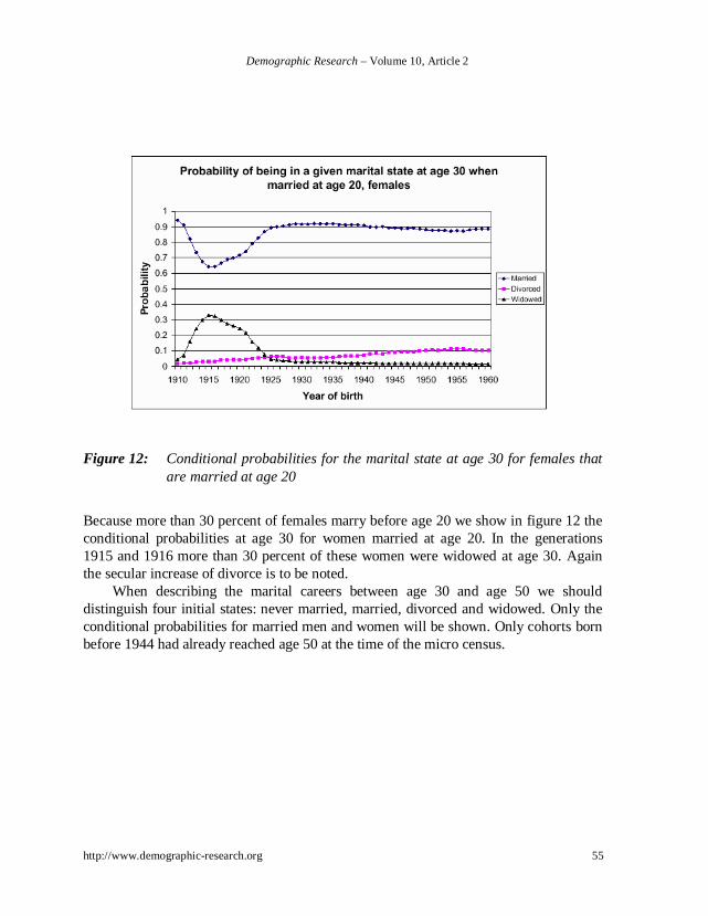
Figure 12: Conditional probabilities for the marital state at age 30 for females thatare married at age 20

Because more than 30 percent of females marry before age 20 we show in figure 12 theconditional probabilities at age 30 for women married at age 20. In the generations1915 and 1916 more than 30 percent of these women were widowed at age 30. Againthe secular increase of divorce is to be noted.

When describing the marital careers between age 30 and age 50 we shoulddistinguish four initial states: never married, married, divorced and widowed. Only theconditional probabilities for married men and women will be shown. Only cohorts bornbefore 1944 had already reached age 50 at the time of the micro census.



Figure 13: Conditional probabilities for the marital state at age 50 for males thatare married at age 30

In figure 13, the history of males married at age 30 (and still alive at the date of themicro census) looks extremely stable. The probability of being married at age 50 ismore than 90 percent. Note that this is not necessarily the same marriage than at age 30.There may have been dissolution(s) and remarriage(s) in the intervening period. Againthe probability of being divorced shows a continuous increase.



Figure 14: Conditional probabilities for the marital state at age 50 for females thatare married at age 30

Again women tell a different story as can be seen from figure 14. In the oldestgenerations nearly 45 percent is widowed at age 50, but in all cohorts widowhood issignificant. A decline of widowhood over the generations is offset by the already notedincrease of divorce. In all generations since 1916 around 80 percent of those married atage 30 is married at age 50.

3. Conclusions

Data on the individual life history of 7 million people were collected in the 1994 microcensus of the Russian Federation. The large size and the representativeness of thesample guarantees that every age group up to around age 90 years for females and age80 for males is represented with enough respondents to permit the reconstruction of partof the demographic history, in particular with respect to marital behavior. Given thepaucity of reliable demographic data on the U.S.S.R. and Russia during most of theperiod between 1926 and 1959 the micro census offers the last opportunity to questionpeople who lived through a large part of the most turbulent part of the history of theSoviet empire.

We can analyze continuity and change in demographic behavior for a large numberof generations in numeric detail, but our data give no information as to changing social,



economic or emotional aspects of marriage, divorce and widowhood. There was atremendous change in education, a growing number of young people got longerschooling in succeeding generations, but the age at first marriage of women, which wasalready low in the oldest generations went down. From around 1936 to 1966 divorcewas very difficult to obtain and the relatively low incidence of divorce in the oldercohorts that reached age 50 before or around 1966 therefore cannot be interpreted as anindicator of the stability of the institution of marriage.

These reservations notwithstanding we could assemble the data on individualmarital events in multistate marital tables for all cohorts born since 1910. Given thelimitations of retrospective data, which only apply for those members of a birth cohortthat are still alive at the date of the micro census, our tables offer the most completedescription of marriage in Russia during most of the 20th century. As far as we knowmultistate marital tables for males were not presented before.

The first conclusion that can be drawn is that some aspects of marital behaviorwere extremely stable over the cohorts we could study. The traditional pattern of earlyand almost universal marriage did not change. The mean age of marriage even declinedfrom an already very low level. The Second World War led to a postponement of firstmarriage and to a remarkably slight increase of the proportion of women nevermarrying in the cohorts most affected.

Divorce became ever more important: in the oldest cohort of 1910 the number ofdivorces per woman was only 0.04 and for men 0.05, but it increased nearly linearly to0.24 for women and 0.21 for men in the cohort 1943. In all later cohorts that could notbe followed up to age 50 we see an increase of divorce: in every succeeding cohort thenumber of divorced males or females at a given age increases. Only in the youngestcohorts there is some stabilization or a small decline (figure 8, 9).

Widowhood is of importance for females only, especially and understandingly forthe women born before 1923 due to the heavy losses during the Second World. War.For the generations born since 1923 the number of times widowed per woman declinesconstantly, which of course is an immediate effect of the decline of mortality in Russia,especially since around 1950.

The collapse of the socialist regimes in the U.S.S.R. and Eastern Europe since1989 and the transition from a planned to a market society, which is still going on, ledto a total change of life, which also will affect demographic behavior. In our data thereis some indication of changes taking place with respect to marriage and divorce, but thedate of the micro census is too early to decide whether this implies a postponement orgenuine structural change. Recent data could imply the latter possibility (Avdeev andMonnier 1999, Philipov 2001).



Notes

1. This study was supported in part by the Netherlands Organization for ScientificResearch (NWO), Project 047-005-020.

2. All computer programs to extract data from the micro census and to performmultistate marital table analysis were developed by S. Scherbov.

3. One of the authors (H.v.V) thanks the Vienna Institute of Demography (IfD) for itshospitality.

4. A preliminary poster version of this paper was presented at the 2000 AnnualMeeting of the Population Association of America in Los Angeles.



References

Andreev, E.L., L. Darsky and T. Kharkova (1998): Demographic history of Russia.Moscow, Informatika [in Russian].

Avdeev, A. and A. Monnier (1999): La nuptialité russe, une complexité méconnue,Population, 54(4-5), 635-676. English translation: Marriage in Russia, acomplex phenomenon poorly understood, Population: an English selection, 12,(2000), 7-50.

Darsky, L. and S. Scherbov (1995): Marital status behavior of women in the formerSoviet Republics. European Journal of Population 11(1), 31-62.

Goskomstat (1995): Goskomstat of Russia, 1994 Microcensus of Russia, topical results(8 volumes). Goskomstat, Moscow [in Russian].

Hajnal, J. (1965): European marriage patterns in perspective, in: D.V. Glass and D.E.D.Eversley (ed), Population in history: essays in historical demography. London,U.K., Arnold, 101-143.

Philipov, D. (2001): Low fertility in Central and Eastern Europe: culture or economy?Paper presented at the IUSSP seminar on ‘International perspectives on lowfertility: trends, theories and policies’, Tokyo, March 21-23, 2001.

Scherbov, S. and H.A.W. van Vianen (1999): Marital and fertility careers of Russianwomen born between 1910 and 1935. Population and Development Review,25(1), 129-143.

Scherbov, S. and H.A.W. van Vianen (2001): Marriage and fertility in Russia of womenborn between 1900 and 1960: a cohort analysis. European Journal ofPopulation, 17(3), 281-294.

Scherbov, S. and H.A.W. van Vianen (2002): Period fertility in Russia since 1930: anapplication of the Coale-Trussell fertility model. Demographic Research, 6(16),454-468.

Volkov, A.G. (1999): Methodology and organization of the 1994 microcensus inRussia. Groningen, Population Research Centre Working Papers 99-5.

Willekens, F. (1987): The marital status life table, in: J. Bongaarts, T.K. Burch andK.W. Wachter (ed), Family demography and their applications. Oxford, U.K.,Clarendon Press, 125-149.

Documents

DEMOGRAPHIC RESEARCH VOLUME 10, ARTICLE 2, … · of peer-reviewed research ... female cohorts confronted with an extreme unbalanced marriage market ... In his seminal article ‘European