Embed Size (px)
Citation preview

Demixed principal component analysis of population
activity in higher cortical areas reveals independent
representation of task parameters
Dmitry Kobak1,*, Wieland Brendel1,2,*, Christos Constantinidis3,Claudia E. Feierstein1, Adam Kepecs4, Zachary F. Mainen1,
Ranulfo Romo5, Xue-Lian Qi3, Naoshige Uchida6, and Christian K. Machens1
1Champalimaud Centre for the Unknown, Lisbon, Portugal2Ecole Normale Superieure, Paris, France
3Wake Forest University School of Medicine, Winston-Salem, NC, USA4Cold Spring Harbor Laboratory, NY, USA
5Universidad Nacional Autonoma de Mexico, Mexico6Harvard University, Cambridge, MA, USA
*Equal contribution
October 2014
Abstract
Neurons in higher cortical areas, such as the prefrontal cortex, are known to be tuned to avariety of sensory and motor variables. The resulting diversity of neural tuning often obscures therepresented information. Here we introduce a novel dimensionality reduction technique, demixedprincipal component analysis (dPCA), which automatically discovers and highlights the essentialfeatures in complex population activities. We reanalyze population data from the prefrontal areas ofrats and monkeys performing a variety of working memory and decision-making tasks. In each case,dPCA summarizes the relevant features of the population response in a single figure. The populationactivity is decomposed into a few demixed components that capture most of the variance in the dataand that highlight dynamic tuning of the population to various task parameters, such as stimuli,decisions, rewards, etc. Moreover, dPCA reveals strong, condition-independent components of thepopulation activity that remain unnoticed with conventional approaches.
Introduction
In many state of the art experiments, a subject, such as a rat or a monkey, performs a behavioral taskwhile the activity of tens to hundreds of neurons in the animal’s brain is monitored using electrophysio-logical or imaging techniques. The common goal of these studies is to relate the external task parameters,such as stimuli, rewards, or the animal’s actions, to the internal neural activity, and to then draw conclu-sions about brain function. This approach has typically relied on the analysis of single neuron recordings.However, as soon as hundreds of neurons are taken into account, the complexity of the recorded dataposes a fundamental challenge in itself. This problem has been particularly severe in higher-order areassuch as the prefrontal cortex, where neural responses display a baffling heterogeneity, even if animals arecarrying out rather simple tasks (Brody et al., 2003; Machens, 2010; Mante et al., 2013; Cunninghamand Yu, 2014).
Traditionally, this heterogeneity has often been ignored. In neurophysiological studies, it is commonpractice to pre-select cells based on particular criteria, such as responsiveness to the same stimulus, andto then average the firing rates of the pre-selected cells. This practice eliminates much of the richness
1
arX
iv:1
410.
6031
v1 [
q-bi
o.N
C]
22
Oct
201
4

of single-cell activities, similar to imaging techniques with low spatial resolution, such as MEG, EEG,or fMRI. While population averages can identify the information that higher-order areas process, theyignore how exactly that information is represented on the neuronal level (Wohrer et al., 2013). Indeed,most neurons in higher cortical areas will typically encode several task parameters simultaneously, andtherefore display what has been termed “mixed selectivity” (Rigotti et al., 2013).
Instead of looking at single neurons and selecting from or averaging over a population of neurons,neural population recordings can be analyzed using dimensionality reduction methods (for a review,see Cunningham and Yu, 2014). In recent years, several such methods have been developed that arespecifically targeted to electrophysiological data, taking into account the binary nature of spike trains(Yu et al., 2009; Pfau et al., 2013), or the dynamical properties of the population response (Buesing et al.,2012; Churchland et al., 2012). However, these approaches reduce the dimensionality of the data withouttaking task parameters, i.e., sensory and motor variables controlled or monitored by the experimenter,into account. Consequently, mixed selectivity remains in the data even after the dimensionality reductionstep, impeding interpretation of the results.
A few recent studies have sought to solve these problems by developing methods that reduce thedimensionality of the data in a way that is informed by the task parameters (Machens, 2010; Machenset al., 2010; Brendel et al., 2011; Mante et al., 2013). One possibility is to adopt a parametric approach,i.e. to assume a specific (e.g. linear) dependency of the firing rates on the task parameters, and thenuse regression to construct variables that demix the task components (Mante et al., 2013). While thismethod can help to sort out the mixed selectivities, it still runs the risk of missing important structuresin the data if the neural activities do not conform to the dependency assumptions (e.g. because ofnonlinearities).
Here, we follow an alternative route by developing an unbiased dimensionality reduction techniquethat fulfills two constraints. It aims to find a decomposition of the data into latent components that(a) are easily interpretable with respect to the experimentally controlled and monitored task parame-ters; and (b) preserve the original data as much as possible, ensuring that no valuable information isthrown away. Our method, which we term demixed principal component analysis (dPCA), improves ourearlier methodological work (Machens, 2010; Machens et al., 2010; Brendel et al., 2011) by eliminatingunnecessary orthogonality constraints on the decomposition. In contrast to several recently suggestedalgorithms for decomposing firing rates of individual neurons into demixed parts (Pagan and Rust, 2014;Park et al., 2014), our focus is on dimensionality reduction.
There is no a priori guarantee that neural population activities can be linearly demixed into latentvariables that reflect individual task parameters. Nevertheless, we applied dPCA to spike train recordingsfrom monkey prefrontal cortex (PFC) (Romo et al., 1999; Qi et al., 2011) and from rat orbitofrontalcortex (OFC) (Feierstein et al., 2006; Kepecs et al., 2008), and obtained remarkably successful demixing.In each case, dPCA automatically summarizes all the important, previously described features of thepopulation activity in a single figure. Importantly, our method provides an easy visual comparisonof complex population data across different tasks and brain areas, which allows us to highlight bothsimilarities and differences in the neural activities. Demixed PCA also reveals several hitherto largelyignored features of population data: (1) most of the activity in these datasets is not related to any ofthe controlled task parameters, but depends only on time (“condition-independent activity”); (2) allmeasured task parameters can be extracted with essentially orthogonal linear readouts; and (3) task-relevant information is shifted around in the neural population space, moving from one component toanother during the course of the trial.
Results
Demixed Principal Component Analysis (dPCA)
We illustrate our method with a toy example (Figure 1). Consider a standard experimental paradigmin which a subject is first presented with a stimulus and then reports a binary decision. The firing ratesof two simulated neurons are shown in Figure 1A. The first neuron’s firing rate changes with time, withstimulus (at the beginning of the trial), and with the animal’s decision (at the end of the trial). Thesecond neuron’s firing rate also changes with time, but only depends on the subject’s decision (not on thestimulus). As time progresses within a trial, the joint activity of the two neurons traces out a trajectory
2

B
C
D
A E
F
Individual neurons
Firi
ng
rate
Stimulus 1Stimulus 2Stimulus 3
Decision: yesDecision: no
Population activity
Firing rateof neuron 1
Firing rateof neuron 2
Stimulu
s 1
Stimulu
s 2
Stimulu
s 3
t=0
t=1t=2
t=3
Time Time
Neuron 1 Neuron 2
PCA
PCA dPCA
Principalaxis 1
Principalaxis 2
dPCA
Encodingaxis: time
Decoder Encoder
Neurons ReconstructedneuronsDemixed
principalcomponents
Decoder Encoder
Neurons Reconstructedneurons
Principalcomponents
Encodingaxis: stimulus
Decodingaxis: time
Decodingaxis: stimulus
Figure 1. Standard and demixed principal component analyses. (A) Time-varying firing rates of two neuronsin a simple stimulus-decision task. Each subplot shows one neuron. Each line shows one condition, with colourcoding the stimulus and solid/dashed line coding the binary decision. (B) Sketch of the population firing rate. Atany given moment in time, the population firing rate of N neurons is represented by a point in an N -dimensionalspace; here N = 2. Each trial is represented by a trajectory in this space. Different experimental conditions (e.g.different stimuli) lead to different average trajectories. Here, colours indicate the different stimuli and dot sizesrepresent the time points. The decision period is not shown for visual clarity. (C) Principal component analysis(PCA). The firing rates of the neurons are linearly transformed (with a “decoder”) into a few latent variables(known as principal components). A second linear transformation (“encoder”) can reconstruct the originalfiring rates from these principal components. PCA finds the decoder/encoder transformations that minimize thereconstruction error. Shades of grey inside each neuron/component show the proportion of variance due to thevarious task parameters (e.g. stimulus, decision, and time), illustrating the “mixed selectivity” of both, neuronsand principal components. Variance terms due to parameter interactions are omitted for clarity. (D) Geometricintuition behind PCA. Same set of points as in (B). The lines show the first two principal axes, the longer onecorresponds to the principal component explaining more variance (the first PC). These two axes form both thedecoder and the encoder, which in case of PCA are identical. (E) Demixed principal component analysis (dPCA).As in PCA, the firing rates are compressed and decompressed through two linear transformations. However, herethe transformations are found by both minimizing the reconstruction error and enforcing a demixing constrainton the latent variables. (F) Geometric intuition behind dPCA. Same set of points as in (B,D), now labeled withtwo parameters: stimulus (colour), and time (dot size); decision is ignored for simplicity. The dashed lines showthe decoding axes, i.e., the axes on which points are projected such that the task-parameter dependencies aredemixed. Solid lines show the encoding axes, i.e., the axes along which the demixed principal components needto be re-expanded in order to reconstruct the original data.
3
in the space of firing rates (Figure 1B; decision not shown for visual clarity). More generally, firing ratesof a population of N neurons at any moment in time is represented by a point in an N -dimensionalspace.
One of the standard approaches to reduce the dimensionality of complex, high-dimensional datasetsis principal component analysis (PCA). In PCA, the original data (here, firing rates of the neurons) arelinearly transformed into several latent variables, called principal components. Each principal componentis therefore a linear combination, or weighted average, of the actual neurons. We interpret these principalcomponents as linear “read-outs” from the full population (Figure 1C, “decoder” D). This transformationcan be viewed as a compression step, as the number of informative latent variables is usually much smallerthan the original dimensionality. The resulting principal components can then be de-compressed withanother linear mapping (“encoder” F), approximately reconstructing the original data. Geometrically,when applied to a cloud of data points (Figure 1D), PCA constructs a set of directions (principal axes)that consecutively maximize the variance of the projections; these axes form both the decoder and theencoder.
More precisely, given a data matrix X, in which each row contains the firing rates of one neuron forall task conditions, PCA finds decoder and encoder that minimize the loss function
LPCA = ‖X− FDX‖2
under the constraint that the principal axes are normalized and orthogonal, and therefore D = F>
(Hastie et al., 2009, section 14.5). However, applying PCA to a neural dataset like the one sketchedin Figure 1A generally results in principal components exhibiting mixed selectivity: many componentswill vary with time, stimulus, and decision (see examples below). Indeed, information about the taskparameters does not enter the loss function.
To circumvent this problem, we sought to develop a new method by introducing an additional con-straint: the latent variables should not only compress the data optimally, but also demix the selectivities(Figure 1E). As in PCA, compression is achieved with a linear mapping D and decompression with alinear mapping F. Unlike PCA, the decoding axes are not constrained to be orthogonal to each other andmay have to be non-orthogonal, in order to comply with demixing. The geometrical intuition is presentedin Figure 1F. Here, the same cloud of data points as in Figures 1B and 1D has labels corresponding totime and stimulus. When we project the data onto the time-decoding axis, information about time ispreserved while information about stimulus is lost, and vice versa for the stimulus-decoding axis. Hence,projections on the decoding axes demix the selectivities. Since the data have been projected onto a non-orthogonal (affine) coordinate system, the optimal reconstruction of the data requires a de-compressionalong a different set of axes, the encoding axes (which implies that D ≈ F+, the pseudo-inverse of F,see Methods).
Given the novel demixing constraint, we term our method demixed PCA (dPCA), and provide adetailed mathematical account in the Methods. Briefly, in the toy example of Figure 1, dPCA first splitsthe data matrix into a stimulus-varying part Xs and a time-varying part Xt, so that X ≈ Xt + Xs, andthen finds separate decoder and encoder matrices for stimulus and time by minimizing the loss function
LdPCA = ‖Xs − FsDsX‖2 + ‖Xt − FtDtX‖2.
See Methods for a more general case.
Somatosensory working memory task in monkey PFC
We first applied dPCA to recordings from the PFC of monkeys performing a somatosensory workingmemory task (Romo et al., 1999; Brody et al., 2003). In this task, monkeys were required to discriminatetwo vibratory stimuli presented to the fingertip. The stimuli were separated by a 3 s delay, and themonkeys had to report which stimulus had a higher frequency by pressing one of two available buttons(Figure 2A). Here, we focus on the activity of 832 prefrontal neurons from two animals, see Methods.For each neuron, we obtained the average time-dependent firing rate (also known as peri-stimulus timehistogram, PSTH) in 12 conditions: 6 values of stimulus frequency F1, each paired with 2 possibledecisions of the monkey. We only analyzed correct trials, so that the decision of the monkey alwayscoincided with the actual trial type (F2>F1 or F1>F2).
4
0 1 2 3 4−400
−200
0
200
400
Time (s)
Nor
mal
ized
firin
g ra
te (
Hz)
−100
−50
0
50
100
−100
0
100
0 1 2 3 4
−100
0
100
Time (s)
1 5 10 150
2
4
6
8
10
Com
pone
nt v
aria
nce
(%)
1 5 10 15
40
60
80
100
Component
Cum
ulat
ive
expl
aine
dsi
gnal
var
ianc
e (%
)
Component
Com
pone
nt
1 5 10 15
1
5
10
15
−1 −0.5 0 0.5 1
Stimulus: 6%Decision: 5%
Condition-independent: 91%
Condition-ind.
Stimulus
Decision
Interaction
34 Hz30 Hz26 Hz18 Hz14 Hz10 Hz
F1 < F2 F1 > F2
1 2 3
6 10 11
5 12 24
16
PCA
dPCA
Stimulus Stimulus
0.5 s 3.0 s 0.5 s
A
C
D
E
B
F1
Dot productsbetween axes
Correlationsbetween
components
F1 F2
28 16
0 1 2 3 4Time (s)
0 1 2 3 4Time (s)
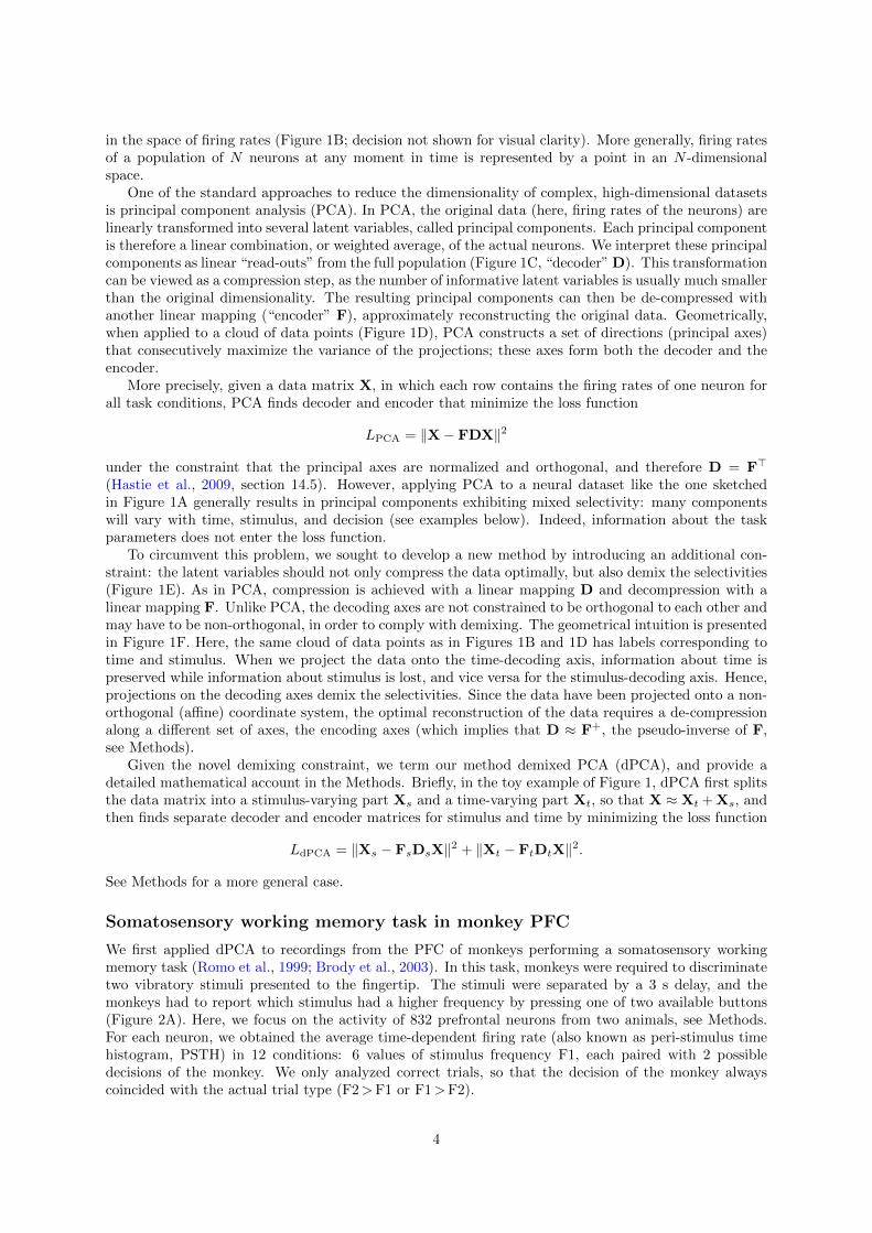
Figure 2. Demixed PCA applied to recordings from monkey PFC during a somatosensory working memorytask (Romo et al., 1999). (A) Cartoon of the paradigm, adapted from (Romo and Salinas, 2003). (B) Demixedprincipal components. Top row: first three condition-independent components; second row: first three stimuluscomponents; third row: first three decision components; last row: first stimulus/decision interaction component.In each subplot there are 12 lines corresponding to 12 conditions (see legend). Thick black lines show timeintervals during which the respective task parameters can be reliably extracted from single-trial activity (seeMethods). Note that the vertical scale differs across rows. (C) Cumulative signal variance explained by PCA(black) and dPCA (red). Demixed PCA explains almost the same amount of variance as standard PCA. (D)Variance of the individual demixed principal components. Each bar shows the proportion of total variance,and is composed out of four stacked bars of different colour: gray for condition-independent variance, blue forstimulus variance, red for decision variance, and purple for variance due to stimulus-decision interactions. Eachbar appears to be single-colored, which signifies nearly perfect demixing. Pie chart shows how the total signalvariance is split between parameters. (E) Upper-right triangle shows dot products between all pairs of the first 15demixed principal axes. Stars mark the pairs that are significantly and robustly non-orthogonal (see Methods).Bottom-left triangle shows correlations between all pairs of the first 15 demixed principal components. Most ofthe correlations are close to zero.
5

As is typical for PFC, each neuron has a distinct response pattern and many neurons show mixedselectivity (Figure S1). Several previous studies have sought to make sense of these heterogeneousresponse patterns by separately analyzing different task periods, such as the stimulation and delayperiods (Romo et al., 1999; Brody et al., 2003; Machens et al., 2010; Barak et al., 2010), the decisionperiod (Jun et al., 2010), or both (Hernandez et al., 2010). With dPCA, however, we can summarize themain features of the neural activity across the whole trial in a single figure (Figure 2B). Just as in PCA,we can think of these demixed principal components as the “building blocks” of the observed neuralactivity, in that the activity of each single neuron is a linear combination (weighted average) of thesecomponents. These building blocks come in four distinct categories: some are condition-independent(Figure 2B, top row); some depend only on stimulus F1 (second row); some depend only on decision(third row); and some depend on stimulus and decision together (bottom row). The components in thefirst three categories demix the parameter dependencies, which is exactly what dPCA aimed for. Westress that applying standard PCA to the same dataset leads to components that strongly exhibit mixedselectivity (Figure S2; see Methods for quantification).
What can we learn about the population activity from the dPCA decomposition? First, we findthat information about the stimulus and the decision can be fully demixed at the population level, eventhough it is mixed at the level of individual neurons. Importantly, the demixing procedure is linear, sothat all components could in principle be retrieved by the nervous system through synaptic weighting anddendritic integration of the neurons’ firing rates. Note that our ability to linearly demix these differenttypes of information is a non-trivial feature of the data.
Second, we see that most of the variance of the neural activity is captured by the condition-independent components (Figure 2B, top row) that together amount to ∼90% of the signal variance(see the pie chart in Figure 2D and Methods). These components capture the temporal modulations ofthe neural activity throughout the trial, irrespective of the task condition. Their striking dominance inthe data may come as a surprise, as such condition-independent components are usually not analyzedor shown. Previously, single-cell activity in the delay period related to these components has often beendubbed “ramping activity” or “climbing activity” (Durstewitz, 2004; Rainer et al., 1999; Komura et al.,2001; Brody et al., 2003; Janssen and Shadlen, 2005; Machens et al., 2010); however, analysis of the fulltrial here shows that the temporal modulations of the neural activity are far more complex and varied.Indeed, they spread out over many components. The origin of these components can only be conjectured,see Discussion.
Third, our analysis also captures the major findings previously obtained with these data: the per-sistence of the F1 tuning during the delay period — component #6 (Romo et al., 1999; Machens et al.,2005), the temporal dynamics of short-term memory — components ##6, 10, 11 (Brody et al., 2003;Machens et al., 2010; Barak et al., 2010), the ramping activities in the delay period — components##1–3, 6 (Singh and Eliasmith, 2006; Machens et al., 2010); and pronounced decision-related activities— component #5 (Jun et al., 2010). We note that the decision components resemble derivatives of eachother; these higher-order derivatives likely arise due to slight variations in the timing of responses acrossneurons (Figure S3).
Fourth, we observe that the three stimulus components show the same monotonic (“rainbow”) tuningbut occupy three distinct time periods: one is active during the S1 period (#10), one during the delayperiod (#6), and one during the S2 period (#11). Information about the stimulus is therefore shiftedaround in the high-dimensional firing rate space. Indeed, if the stimulus were always encoded in thesame subspace, there would only be a single stimulus component. In other words, if we perform dPCAanalysis in a short sliding time window, then the main stimulus axis will rotate with time instead ofremaining constant.
We furthermore note several important technical points. First, the overall variance explained bythe dPCA components (Figure 2C, red line) is very close to the overall variance captured by the PCAcomponents (Figure 2C, black line). This means that by imposing the demixing constraint we did notlose much of the variance, and so the population activity is accurately represented by the obtaineddPCA components (Figure 2B). Second, as noted above, the demixed principal axes are not constrainedto be orthogonal. Nonetheless, most of them are quite close to orthogonal (Figure 2E, upper-righttriangle). There are a few notable exceptions, which we revisit in the Discussion section. Third, pairwisecorrelations between components are all close to zero (Figure 2E, lower-left triangle), as should beexpected as the components are considered to represent independent signals.
6

0 1 2 3 4−150
−100
−50
0
50
100
150
Time (s)
−50
0
50
−15
−10
−5
0
5
10
15
0 1 2 3 4−60
−40
−20
0
20
40
60
Time (s)0 1 2 3 4
Time (s)
20
40
60
80
14
1 5 10 150
2
4
6
8
10
Com
pone
nt v
aria
nce
(%)
1 5 10 15Component
Cum
ulat
ive
expl
aine
dsi
gnal
var
ianc
e (%
)
Component
Com
pone
nt
1 5 10 15
1
5
10
15
−1 −0.5 0 0.5 1
A
C
D
E
B
Stimulus: 20%
Decision: 1%
Condition-independent: 76%
Interaction: 4%N
orm
aliz
ed fi
ring
rat
e (H
z)
Condition-ind.
Stimulus
Decision
Interaction
0 1 2 3 4Time (s)
1 2 3
7 8 9
21 40
10 13preferred45° away90° away
135° awayopposite
match non-matchF1
Stimulus Stimulus
0.5 s 1.5 s 0.5 s
S1 S2
Cue
1.5 s+
PCA
dPCA
Dot productsbetween axes
Correlationsbetween
components
Figure 3. Demixed PCA applied to recordings from monkey PFC during a visuospatial working memory task(Qi et al., 2011). Same format as Figure 2. (A) Cartoon of the paradigm, adapted from (Romo and Salinas,2003). (B) Demixed principal components. In each subplot there are 10 lines corresponding to 10 conditions(see legend). Colour corresponds to the position of the last shown stimulus (first stimulus for t < 2 s, secondstimulus for t > 2 s). In non-match conditions (dashed lines) the colour changes at t = 2 s. Solid lines correspondto match conditions and do not change colours. (C) Cumulative signal variance explained by PCA and dPCAcomponents. (D) Variance of the individual demixed principal components. Pie chart shows how the total signalvariance is split between parameters. (E) Upper-right triangle shows dot products between all pairs of the first 15demixed principal axes, bottom-left triangle shows correlations between all pairs of the first 15 demixed principalcomponents.
Visuospatial working memory task in monkey PFC
We next applied dPCA to recordings from the PFC of monkeys performing a visuospatial workingmemory task (Qi et al., 2011; Meyer et al., 2011; Qi et al., 2012). In this task, monkeys first fixated ata small white square at the centre of a screen, when a square S1 appeared in one of the eight locationsaround the centre (Figure 3A). After a 1.5 s delay, a second square S2 appeared in either the same(“match”) or the opposite (“non-match”) location. Following another 1.5 s delay, a green and a bluechoice targets appeared in locations orthogonal to the earlier presented stimuli. Monkeys had to saccadeto the green target to report a match condition, and to the blue one to report a non-match.
We analyzed the activity of 956 neurons recorded in the lateral PFC of two monkeys performing thistask. Proceeding exactly as before, we obtained the average time-dependent firing rate of each neuronfor each condition. Following the original studies, we eliminated the trivial rotational symmetry of thetask by collapsing the eight possible stimulus locations into five locations that are defined with respectto the preferred direction of each neuron (0◦, 45◦, 90◦, 135◦, or 180◦ away from the preferred direction,see Methods). As a consequence, we obtained 10 conditions: 5 possible stimulus locations, each pairedwith 2 possible decisions of the monkey. We again only analyzed correct trials, so that the decision ofthe monkey always coincided with the actual trial type.
The dPCA results are shown in Figure 3. Just as before, the components fall into four categories:they can be condition-independent (Figure 3B, top row); dependent only on stimulus location (secondrow); only on decision (third row); or dependent on stimulus-decision interactions (bottom row).
7

We note several similarities to the somatosensory working memory task. First, stimulus and decisioncan be separated at the population level just as easily as before, despite being intermingled at the single-neuron level. Second, most of the variance in the neural activity is again captured by the condition-independent components (Figure 3B, top row, and 3D, pie chart). Third, all stimulus components areactive in different time periods, and the same is true for the decision, indicating rotation of the stimulusand decision representations in the firing rate space. Fourth, and maybe most surprisingly, we find thatthe overall structure of population activity up to the second stimulus (S2) is almost identical to thatfound in the somatosensory task. In both cases, the leading condition-independent components are quitesimilar (compare Figure 2B with Figure 3B). Furthermore, in both tasks we find a stimulus componentwith strong activity during the F1/S1 period, a stimulus component with persistent activity during thedelay period, and a decision component with activity during the F2/S2 period.
One notable difference between Figures 2 and 3 is the presence of strong interaction components inFigure 3B. However, interaction components in Figure 3B are in fact stimulus components in disguise.In match trials, S2 and S1 appear at the same location, and in non-match trials at opposite locations.Information about S2 is therefore given by a non-linear function of stimulus S1 and the trial type (i.e.decision), which is here captured by the interaction components.
The differences in the population activity between these two tasks seem to stem mostly from thespecifics of the tasks, such as the existence of a second delay period in the visuospatial working memorytask. There are also differences in the overall amount of power allocated to different components, withthe stimulus (and interaction) components dominating in the visuospatial working memory task, whereasstimulus and decision components are more equally represented in the somatosensory task. However, theoverall structure of the data is surprisingly similar.
Here again, our analysis summarizes previous findings obtained with this dataset. For instance, thefirst and the second decision components show tuning to the match/non-match decision in the delayperiod between S2 and the cue (first component) and during the S2 period (second component). Usingthese components as fixed linear decoders, we achieve cross-validated single-trial classification accuracy ofmatch vs. non-match of ∼75% for t > 2 (Figure S4), which is approximately equal to the state-of-the-artclassification performance reported previously (Meyers et al., 2012).
Constantinidis et al. have also recorded population activity in PFC before starting the training (bothS1 and S2 stimuli were presented exactly as above, but there were no cues displayed and no decisionrequired). When analyzing this pre-training population activity with dPCA, the first stimulus and thefirst interaction components come out close to the ones shown on Figure 3, but there are no decisionand no “memory” components present (Figure S5), in line with previous findings (Meyers et al., 2012).These task-specific components appear in the population activity only after extensive training.
Olfactory discrimination task in rat OFC
Next, we applied dPCA to recordings from the OFC of rats performing an odour discrimination task(Feierstein et al., 2006). This behavioral task differs in two crucial aspects from the previously consideredtasks: it requires no active storage of a stimulus, and it is self-paced. To start a trial, rats entered anodour port, which triggered delivery of an odour with a random delay of 0.2–0.5 s. Each odour wasuniquely associated with one of the two available water ports, located to the left and to the right fromthe odour port (Figure 4A). Rats could sample the odour for as long as they wanted up to 1 s, andthen had to move to one of the water ports. If they chose the correct water port, reward was deliveredfollowing an anticipation period of random length (0.2–0.5 s).
We analyzed the activity of 437 neurons recorded in five rats in 4 conditions: 2 stimuli (left and right)each paired with 2 decisions (left and right). Two of these conditions correspond to correct (rewarded)trials, and two correspond to error (unrewarded) trials. Since the task was self-paced, each trial had adifferent length; in order to align events across trials, we restretched the firing rates in each trial (seeMethods). Alignment methods without restretching led to similar results (Figure S6).
Just as neurons from monkey PFC, neurons in rat OFC exhibit diverse firing patterns and mixedselectivity (Feierstein et al., 2006). Nonetheless, dPCA is able to demix the population activity, resultingin the condition-independent, stimulus, decision, and interaction components (Figure 4). In this dataset,interaction components separate rewarded and unrewarded conditions (thick and thin lines on Figure4B, bottom row), i.e., correspond to neurons tuned either to reward, or to the absence of reward.
8
0 1 2 3 4
−100
−50
0
50
100
Time (s)
−20
−10
0
10
20
−50
0
50
0 1 2 3 4−60
−40
−20
0
20
40
60
Time (s)0 1 2 3 4
Time (s)0 1 2 3 4
Time (s)
20
40
60
80
100
25
−25
1 5 10 150
2
4
6
8
10
Com
pone
nt v
aria
nce
(%)
1 5 10 15Component
Cum
ulat
ive
expl
aine
dsi
gnal
var
ianc
e (%
)
Component
Com
pone
nt
1 5 10 15
1
5
10
15
−1 −0.5 0 0.5 1
A
C
D
E
B
Nor
mal
ized
firi
ng r
ate
(Hz)
Condition-ind.
Stimulus
Decision
Interaction
Odour port Reward port
Antici
patio
npe
riod
Stimulus: 2%Decision: 7%
Condition-independent: 78%
Interaction: 13%
PCA
dPCA
28 18RightLeft
Rightchoice
Leftchoice
Odour
rewarded
conditions
Odourport
Rightchoice
Leftchoice
1 2 3
11 21
7 10 13
4 9 14
Dot productsbetween axes
Correlationsbetween
components
CH3CH3H3C
O
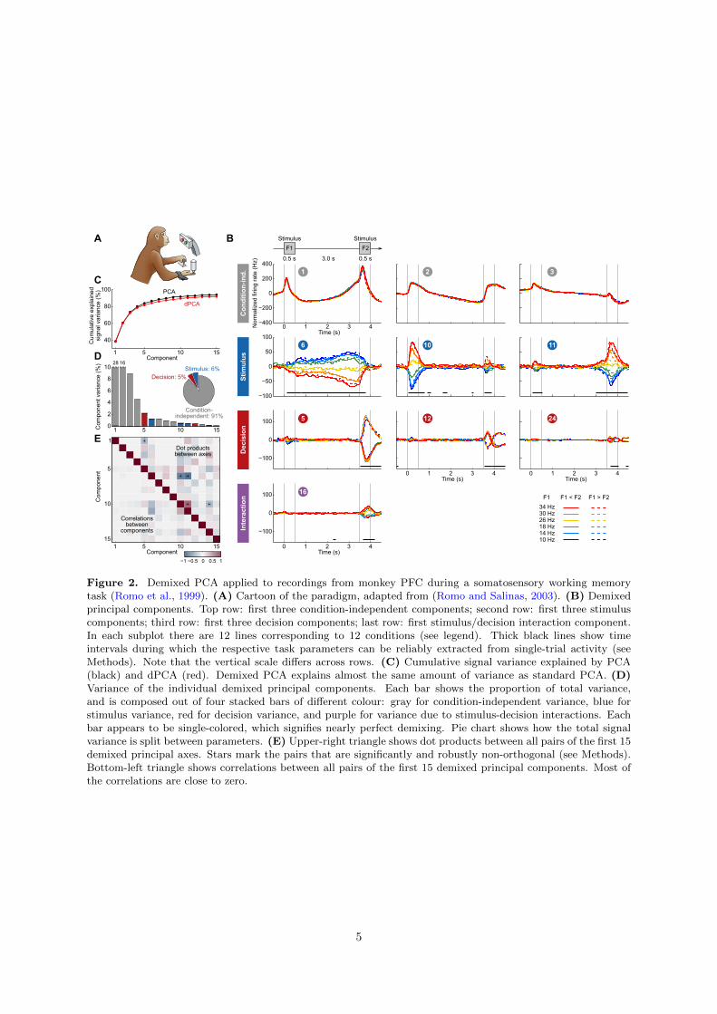
Figure 4. Demixed PCA applied to recordings from rat OFC during an olfactory discrimination task (Feiersteinet al., 2006). Same format as Figure 2. (A) Cartoon of the paradigm, adapted from (Wang et al., 2013).(B) Each subplot shows one demixed principal component. In each subplot there are 4 lines correspondingto 4 conditions (see legend). Two out of these four conditions were rewarded and are shown by thick lines.(C) Cumulative variance explained by PCA and dPCA components. (D) Variance of the individual demixedprincipal components. Pie chart shows how the total signal variance is split between parameters. (E) Upper-righttriangle shows dot products between all pairs of the first 15 demixed principal axes, bottom-left triangle showscorrelations between all pairs of the first 15 demixed principal components.
We note several similarities to the monkey PFC data. The largest part of the total variance is againdue to the condition-independent components (over 60% of the total variance falls into the first threecomponents). Also, for both stimulus and decision, the main components are localized in distinct timeperiods, meaning that information about the respective parameters is shifted around in firing rate space.
The overall pattern of neural tuning across task epochs that we present here agrees with the findingsof the original study (Feierstein et al., 2006). Interaction components are by far the most prominentamong all the condition-dependent components, corresponding to the observation that many neuronsare tuned to presence/absence of reward. Decision components come next, with a caveat that decisioninformation may also reflect the rat’s movement direction and/or position, as was pointed out previously(Feierstein et al., 2006). Stimulus components are less prominent, but nevertheless show clear stimulustuning, demonstrating that even in error trials there is reliable information about stimulus identity inthe population activity.
Finally, we note that the first interaction component (#4) shows significant tuning to reward alreadyin the anticipation period. In other words, neurons tuned to presence/absence of reward start firingbefore the reward delivery (or, on error trials, before the reward could have been delivered). We returnto this observation in the next section.
Olfactory categorization task in rat OFC
Kepecs et al. (2008) extended the experiment of Feierstein et al. (2006) by using odour mixtures insteadof pure odours, thereby varying the difficulty of each trial (Uchida and Mainen, 2003; Kepecs et al.,2008). In each trial, rats experienced mixtures of two fixed odours with different proportions (Figure
9

0 1 2 3 4
−50
0
50
Time (s)
−10
0
10
−20
−10
0
10
20
0 1 2 3 4−50
0
50
Time (s)0 1 2 3 4
0 1 2 3 4Time (s)
20
40
60
80
100
0
2
4
6
8
10
Com
pone
nt v
aria
nce
(%)
1 5 10 15Component
Cum
ulat
ive
expl
aine
dsi
gnal
var
ianc
e (%
)
Component
Com
pone
nt
1 5 10 15
1
5
10
15
−1 −0.5 0 0.5 1
A
C
D
E
B
Nor
mal
ized
firi
ng r
ate
(Hz)
Condition-ind.
Stimulus
Decision
Interaction
Odour port Reward port
Antici
patio
npe
riod
Stimulus: 3%Decision: 7%
Condition-independent: 70%
Interaction: 21%
Odourport
Rightchoice
Leftchoice
1 2 4
11 17
8 13 14
3 6
1 5 10 15
PCA
dPCA
26 13100%68%56%44%32%0%
Left
0%32%44%56%68%
100%
Right
OdoursRight
choiceLeft
choice
rewarded
conditions
0 50 100−20
0
20
Time (s) Odour (% right)
Average overanticipation period
Wrong
Correct
Dot productsbetween axes
Correlationsbetween
components
CH3CH3H3C
O
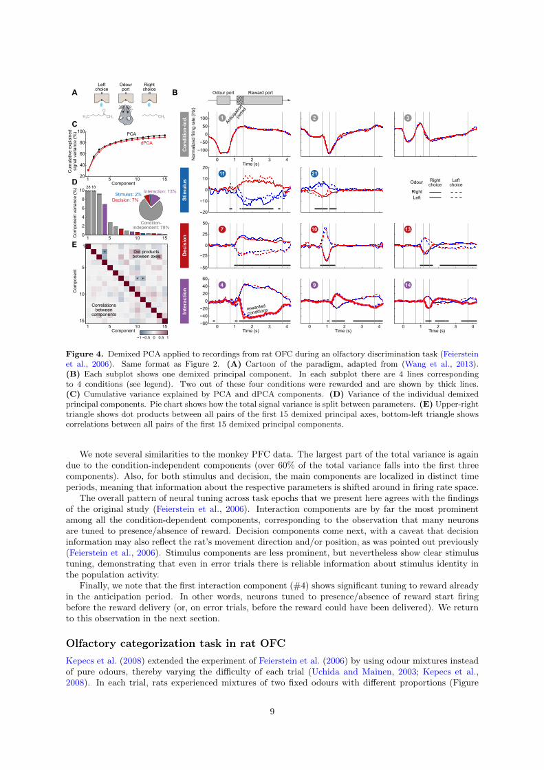
Figure 5. Demixed PCA applied to recordings from rat OFC during an olfactory categorization task (Kepecset al., 2008). Same format as Figure 2. (A) Cartoon of the paradigm, adapted from (Wang et al., 2013). (B)Each subplot shows one demixed principal component. In each subplot there are 10 lines corresponding to 10conditions (see legend). Six out of these 10 conditions were rewarded and are shown with thick lines; note thatthe pure left (red) and the pure right (blue) odours did not have error trials. Inset shows mean rate of the secondinteraction component during the anticipation period. (C) Cumulative variance explained by PCA and dPCAcomponents. (D) Variance of the individual demixed principal components. Pie chart shows how the total signalvariance is split between parameters. (E) Upper-right triangle shows dot products between all pairs of the first 15demixed principal axes, bottom-left triangle shows correlations between all pairs of the first 15 demixed principalcomponents.
5A). Left choices were rewarded if the proportion of the “left” odour was above 50%, and right choicesotherwise. Furthermore, the waiting time until reward delivery (anticipation period) was increased to0.3–2 s.
We analyzed the activity of 214 OFC neurons from three rats recorded in 8 conditions, correspondingto 4 odour mixtures, each paired with 2 decisions (left and right). During the presentation of pure odours(100% right and 100% left) rats made essentially no mistakes, and so we had to exclude these data fromthe dPCA computations (which require that all parameter combinations are present, see Methods).Nevertheless, we displayed these additional 2 conditions in Figure 5.
The dPCA components shown in Figure 5B are similar to those presented above in Figure 4B.The condition-independent components capture most of the total variance; the interaction components(corresponding to the reward) are most prominent among the condition-dependent ones; the decisioncomponents are somewhat weaker and show tuning to the rat’s decision, starting from the odour portexit and throughout the rest of the trial; and the stimulus components are even weaker, but again reliable.
Here again, some of the interaction components (especially the second one, #6) show strong tuningalready during the anticipation period, i.e. before the actual reward delivery. The inset in Figure 5Bshows the mean value of the component #6 during the anticipation period, separating correct (green)and incorrect (red) trials for each stimulus. The characteristic U-shape for the error trials and theinverted U-shape for the correct trials agrees well with the predicted value of the rat’s uncertainty ineach condition (Kepecs et al., 2008). Accordingly, this component can be interpreted as correspondingto the rat’s uncertainty or confidence about its own choice, confirming the results of Kepecs et al. (2008).
10
In summary, both the main features of this dataset, as well as some of the subtleties that have beenpointed out before (Kepecs et al., 2008) are picked up and reproduced by dPCA.
Distribution of components in the neural population
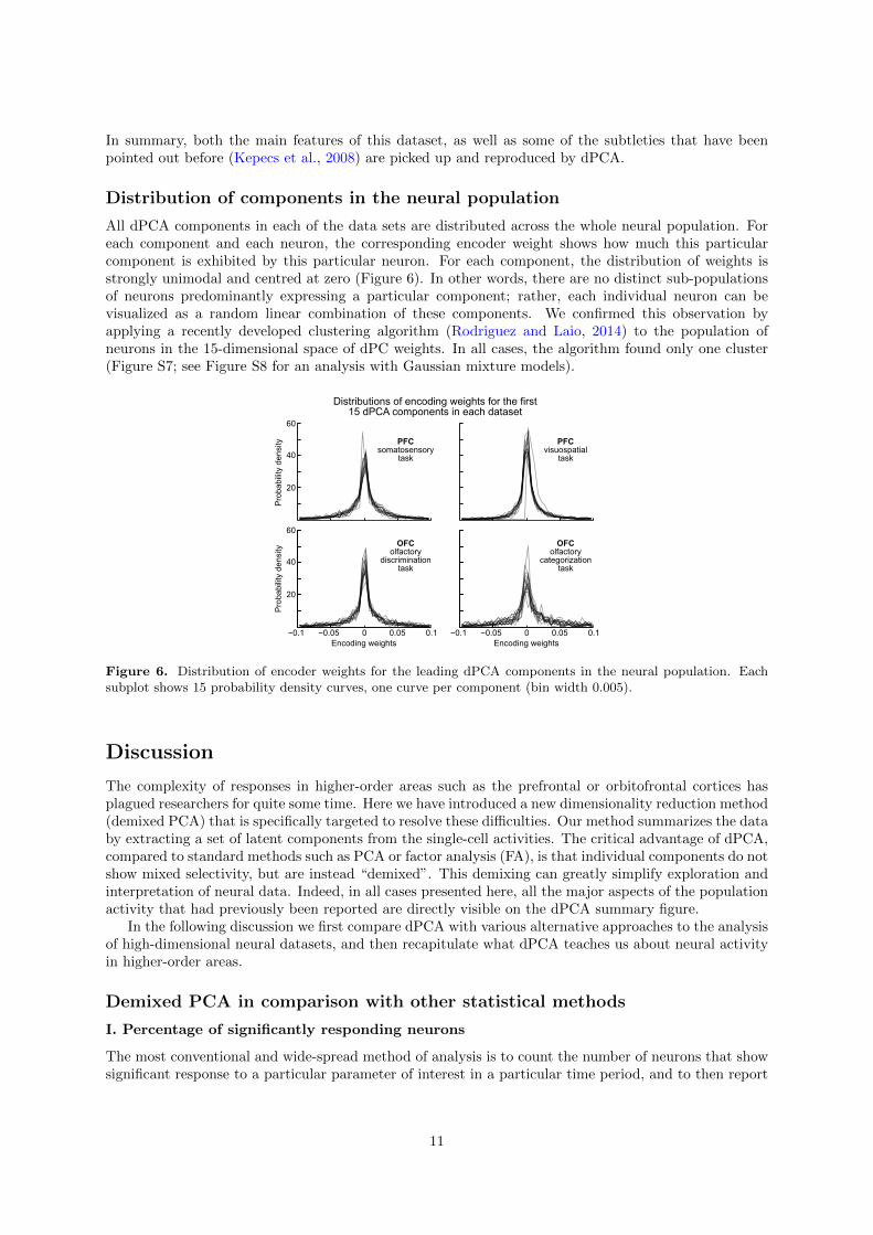
All dPCA components in each of the data sets are distributed across the whole neural population. Foreach component and each neuron, the corresponding encoder weight shows how much this particularcomponent is exhibited by this particular neuron. For each component, the distribution of weights isstrongly unimodal and centred at zero (Figure 6). In other words, there are no distinct sub-populationsof neurons predominantly expressing a particular component; rather, each individual neuron can bevisualized as a random linear combination of these components. We confirmed this observation byapplying a recently developed clustering algorithm (Rodriguez and Laio, 2014) to the population ofneurons in the 15-dimensional space of dPC weights. In all cases, the algorithm found only one cluster(Figure S7; see Figure S8 for an analysis with Gaussian mixture models).
−0.1 −0.05 0 0.05 0.1
20
40
60
Distributions of encoding weights for the first15 dPCA components in each dataset
−0.1 −0.05 0 0.05 0.1
20
40
60
PFCsomatosensory
task
PFCvisuospatial
task
OFColfactory
discriminationtask
OFColfactory
categorizationtask
Encoding weights Encoding weights
Pro
bab
ility
den
sity
Pro
bab
ility
den
sity
Figure 6. Distribution of encoder weights for the leading dPCA components in the neural population. Eachsubplot shows 15 probability density curves, one curve per component (bin width 0.005).
Discussion
The complexity of responses in higher-order areas such as the prefrontal or orbitofrontal cortices hasplagued researchers for quite some time. Here we have introduced a new dimensionality reduction method(demixed PCA) that is specifically targeted to resolve these difficulties. Our method summarizes the databy extracting a set of latent components from the single-cell activities. The critical advantage of dPCA,compared to standard methods such as PCA or factor analysis (FA), is that individual components do notshow mixed selectivity, but are instead “demixed”. This demixing can greatly simplify exploration andinterpretation of neural data. Indeed, in all cases presented here, all the major aspects of the populationactivity that had previously been reported are directly visible on the dPCA summary figure.
In the following discussion we first compare dPCA with various alternative approaches to the analysisof high-dimensional neural datasets, and then recapitulate what dPCA teaches us about neural activityin higher-order areas.
Demixed PCA in comparison with other statistical methods
I. Percentage of significantly responding neurons
The most conventional and wide-spread method of analysis is to count the number of neurons that showsignificant response to a particular parameter of interest in a particular time period, and to then report
11
the resulting percentage. This method was used in all of the original publications whose data we re-analyzed here: Romo et al. (1999) showed that 65% of the neurons (from those showing any task-relatedresponses) exhibited monotonic tuning to the stimulation frequency during the delay period. Meyer et al.(2011) reported that the percentage of neurons with increased firing rate in the delay period increasedafter training from 15–21% to 27%, and the percentage of neurons tuned to match/non-match differenceincreased from 11% to 21%. Feierstein et al. (2006) found that 29% of the neurons were significantlytuned to reward, and 41% to the rat’s decision. Similarly, Kepecs et al. (2008) found that 42% of theneurons were significantly tuned to reward and observed that in the anticipation period these neuronsdemonstrated tuning to the expected uncertainty level. Note that in all of these cases our conclusionsbased on the dPCA analysis qualitatively agree with these previous findings.
Even though the conventional approach is perfectly sound, it does have several important limitationsthat dPCA is free of:
1. The conventional analysis focuses on a particular time bin (or on the average firing rate over aparticular time period) and therefore provides no information about the time course of neuraltuning. In contrast, dPCA results in time-dependent components, which highlight the time courseof neural tuning.
2. If a parameter has more than two possible values, such as the vibratory frequencies in the so-matosensory working memory task, then reporting a percentage of neurons with significant tuningdisregards the shape of the tuning curve. On the other hand, a vertical slice through any stimulus-dependent dPCA component results in a tuning curve. In the case of “rainbow-like” stimuluscomponents (Figure 2B, 3B, or 5B), these tuning curves are easy to imagine.
3. To count significantly tuned neurons, one chooses an arbitrary p-value cutoff (e.g. p < 0.05).This can potentially create a false impression that neurons are separated into two distinct sub-populations: those tuned to a given parameter (e.g. stimulus) and those that are not tuned.This, however, is not the case in any of the datasets considered here: each demixed component isexpressed in the whole population, albeit with varying strength (Figure 6).
4. If neural tuning to several parameters is analyzed separately (e.g. with several t-tests or several one-way ANOVAs instead of one multi-way ANOVA), then the results of the tests can get confoundeddue to different number of trials in different conditions (“unbalanced” experimental design). Incase of dPCA, all parameters are analyzed together, and the issue of confounding does not arise.
An extended version of this approach uses multi-way ANOVA to test for firing rate modulation dueto several parameters of interest, and repeats the test in a sliding time window to obtain the time courseof neural tuning (see e.g. Sul et al., 2010, 2011). This avoids the first and the fourth limitations listedabove, but the other two limitations still remain.
II. Population averages
In many studies, the time-varying firing rates, or PSTHs, of individual neurons are simply averaged overa subset of the neurons that were found to be significantly tuned to a particular parameter of interest(e.g. Rainer et al., 1999; Kepecs et al., 2008). While this approach can highlight some of the dynamicsof the population response, it ignores the full complexity and heterogeneity of the data (Figure S1),which is largely averaged out. The approach thereby fails to faithfully represent the neural activities,and may lead to the false impression pointed out in the third issue above, namely that there are distinctsubpopulations of neurons with distinct response patterns.
III. Demixing approach based on multiple regression
Mante et al. (2013), have recently introduced a demixing approach based on multiple regression. Theauthors first performed a linear regression of neural firing rates to several parameters of interest, andthen took the vectors of regression coefficients as demixing axes. While this method proved sufficient forthe purposes of that study, it does not aim to faithfully capture all of the data, which leads to severaldisadvantages. Specifically, the approach (a) ignores the condition-independent components, (b) assumesthat all neural tuning is linear, (c) finds only a single demixed component for each parameter, and (d)
12

cannot achieve demixing when the axes for different parameters are far from orthogonal. To illustratethese disadvantages, we applied this method to all our datasets and show the results in Figure S9.
A significant advantage of the approach by Mante et al. (2013), is that it can deal with missing dataor continuous task parameters, which dPCA currently can not. Future extensions of dPCA may thereforeconsider replacing the non-parametric dependencies of firing rates on task parameters with a parametricmodel, which would combine the advantages of both methods.
IV. Decoding approach
Another multivariate approach relies on linear classifiers that predict the parameter of interest from thepopulation firing rates. The strength of neural tuning can then be reported as the cross-validated classi-fication accuracy. For example, Meyers et al. (2012), built linear classifiers for stimulus and match/non-match condition for the visuospatial working memory task analyzed above. Separate classifiers wereused in each time bin, resulting in a time-dependent classification accuracy. The shape of the accuracycurve for the match/non-match condition follows the combined shapes of our decision components (andthe same is true for stimulus). While the time-dependent classification accuracy provides an importantand easily understandable summary of the population activity, it is far removed from the firing rates ofindividual neurons and is not directly representative of the neural tuning. The dPCA approach is moredirect.
V. Linear discriminant analysis
Linear classifiers can also be used to inform the dimensionality reduction. For instance, linear discrim-inant analysis (LDA) reduces the dimensionality of a dataset while taking class labels into account.Whereas PCA looks for linear projections that maximize total variance (and ignores class labels), LDAlooks for linear projections that maximize class separation, i.e. with maximal between-class and minimalwithin-class variance. Consequently, LDA is related to dPCA. However, LDA is a one-way technique(i.e. it considers only one parameter) and is not concerned with reconstruction of the original data,which makes it ill-suited for our purposes. See Supplementary Materials for an extended discussion onthe differences between dPCA and LDA.
Insights obtained from applying dPCA to the four datasets
One interesting outcome of the analysis concerns the strength of the condition-independent components.These components capture 70–90% of the total, task-locked variance of neural firing rates. They arelikely explained in part by an overall firing rate increase during certain task periods (e.g. during stimuluspresentation). More speculatively, they could also be influenced by residual sensory or motor variablesthat vary rhythmically with the task, but are not controlled or monitored (Renart and Machens, 2014).The attentional or motivational state of animals, for instance, often correlates with breathing (Huijberset al., 2014), pupil dilation (Eldar et al., 2013), body movements (Gouvea et al., 2014), etc.
The second important observation is that parameter tuning “moves” during the trial from one compo-nent to another. To visualize these movements, we set up the dPCA algorithm such that it preferentiallyreturns projections occupying only localized periods in time (see Methods). As a result, there are e.g.three separate stimulus components on Figure 2: one is active during the S1 period, one during the delayperiod, and one during the S2 period. The same can be observed in all other data sets as well: considerstimulus components in Figure 3 or decision components in Figures 4–5. The possibility to separatesuch components means that a neural subspace carrying information about a particular task parameter,changes (rotates) with time during the trial.
Our third finding is that most encoding axes turn out to be almost orthogonal to each other (only22 out of 420 pairs are marked with stars on Figures 2–5E), even though dPCA, unlike PCA, does notenforce orthogonality. Non-orthogonality between two axes means that neurons expressing one of thecomponents tend also to express the other one. Most examples of non-orthogonal pairs fall into thefollowing three categories:
1. Non-orthogonality between a condition-dependent component and a condition-independent one (9pairs), e.g. the first interaction (#4) and the second condition-independent (#2) components in
13

Figure 4. This means that the neurons that are tuned to the presence/absence of reward will tendto have a specific time course of firing rate modulation, corresponding to component #2. Notethat the same effect is observed in Figure 5.
2. Non-orthogonality between components describing one parameter (10 pairs), e.g. stimulus compo-nents in Figure 2. As many neurons express all three components, their axes end up being stronglynon-orthogonal.
3. A special example is given by Figure 3, where the first stimulus component (#7) and the firstinteraction component (#10) are strongly non-orthogonal. As the interaction components in thatparticular data set are actually tuned to stimulus S2, this example can be seen a special case ofthe previous category.
Only two pairs do not fall into any of the categories listed above (first stimulus and first decisioncomponents in both olfactory datasets). In all other cases, the condition-dependent components turn outto be almost orthogonal to each other. In other words, task parameters are represented independently ofeach other. Indeed, if latent components are independently, i.e. randomly mapped to a space of neurons,then the encoding axes will be nearly orthogonal to each other, because in a high-dimensional space anytwo random vectors are close to being orthogonal (unlike 2D or 3D cases). Substantial deviations fromorthogonality can only occur if different parameters are encoded in a population in a non-independentway. Our results indicate that this is mostly not the case. In addition to that, orthogonal readoutsare arguably the most effective, as they maximize signal-to-noise ratio, ensuring successful demixing indownstream brain areas.
Limitations
One limitation of dPCA is that it works only with discrete parameters (and all possible parameter com-binations must be present in the data) and would need to be extended to be able to treat continuousparameters as well. Another is that the number of neurons needs to be high enough: we found that atleast ∼100 neurons are usually needed to achieve satisfactory demixing in the data considered here. Fur-thermore, here we worked with trial-averaged PSTHs and ignored trial-to-trial variability. The datasetspresented here could not have been analyzed differently, because the neurons were recorded across mul-tiple sessions, and noise correlations between neurons were therefore not known. Demixed PCA could inprinciple also be used for simultaneous recordings of sufficient dimensionality. However, dPCA does notspecifically address the question of how to properly treat trial-to-trial variability, and this problem mayrequire further extensions in the future.
Outlook
Here we argued that dPCA is an exploratory data analysis technique that is well suited for neural data,as it provides a succinct and immediately accessible overview of the population activity. It is importantto stress its exploratory nature: dPCA enables a researcher to have a look at the full data, ask furtherquestions and perform follow-up analyses and statistical tests. It should therefore be a beginning, notthe end of the analysis.
The dPCA code for Matlab and Python is available at https://github.com/wielandbrendel/dPCA.
14

Materials and Methods
Experimental data
Brief descriptions of experimental paradigms are provided in the Results section and readers are referredto the original publications for all further details. Here we describe the selection of animals, sessions,and trials for the present manuscript. In all experiments neural recordings were obtained in multiplesessions, so most of the neurons were not recorded simultaneously.
1. Somatosensory working memory task in monkeys (Romo et al., 1999; Brody et al., 2003). Weused the data from two monkeys (code names RR14 and RR15) that were trained with the samefrequency set, and selected only the sessions where all six frequencies {10, 14, 18, 26, 30, 34} Hzwere used for the first stimulation (other sessions were excluded). Monkeys made few mistakes(overall error rate was 6%), and here we analyzed only correct trials. Monkey RR15 had additional3 s delay after the end of the second stimulation before it was cued to provide the response. Usingthe data from monkey RR13 (that experienced different frequency set) led to very similar dPCAcomponents (data not shown).
2. Visuospatial working memory task in monkeys (Qi et al., 2011; Meyer et al., 2011; Qi et al., 2012).We used the data from two monkeys (code names AD and EL) that were trained with the samespatial task. Monkeys made few mistakes (overall error rate was 8%), and here we analysed onlycorrect trials. The first visual stimulus was presented at 9 possible spatial locations arranged in a3×3 grid (Figure 3A); here we excluded all the trials where the first stimulus was presented in thecentre position.
3. Olfactory discrimination task in rats (Feierstein et al., 2006). We used the data from all fiverats (code names N1, P9, P5, T5, and W1). Some rats were trained with two distinct odours,some with four, some with six, and one rat experienced mixtures of two fixed odours in varyingproportions. In all cases each odour was uniquely associated with one of the two available waterports (left/right). Following the original analysis (Feierstein et al., 2006), we grouped all odoursassociated with the left/right reward together as a “left/right odour”. For most rats, caproic acidand 1-hexanol (shown on Figures 4–5A) were used as the left/right odour. We excluded from theanalysis all trials that were aborted by rats before reward delivery (or before waiting 0.2 s at thereward port for the error trials).
4. Olfactory categorization task in rats (Kepecs et al., 2008). We used the data from all three rats(code names N1, N48, and N49). Note that recordings from one of the rats (N1) were includedin both this and previous datasets; when we excluded if from either of the datasets, the resultsstayed qualitatively the same (data not shown). We excluded from the analysis all trials that wereaborted by rats before reward delivery (or before waiting 0.3 s at the reward port for the errortrials).
Neural recordings
In each of the datasets each trial can be labeled with two parameters: “stimulus” and “decision”. Notethat a “reward” label is not needed, because its value can be deduced from the other two due to thedeterministic reward protocols in all tasks. For our analysis it is important to have recordings of eachneuron in each possible condition (combination of parameters). Additionally, we required that in eachcondition there were at least Emin > 1 trials, to reduce the standard error of the mean when averagingover trials, and also for cross-validation purposes. The cutoff was set to Emin = 5 for both workingmemory datasets, and to Emin = 2 for both olfactory datasets (due to less neurons available).
We have further excluded very few neurons with mean firing rate over 50 Hz, as neurons with veryhigh firing rate can bias the variance-based analysis. Firing rates above 50 Hz were atypical in all datasets(number of excluded neurons for each dataset: 5 / 2 / 1 / 0). This exclusion had a minor positive effecton the components. We did not apply any variance-stabilizing transformations, but if the square-roottransformation was applied, the results stayed qualitatively the same (data not shown).
15

No other pre-selection of neurons was used. This procedure left 832 neurons (230 / 602 for individualanimals, order as above) in the somatosensory working memory dataset, 956 neurons (182 / 774) in thevisuospatial working memory dataset, 437 neurons in the olfactory discrimination dataset (166 / 30 / 9/ 106 / 126), and 214 neurons in the olfactory categorization dataset (67 / 38 / 109).
Preprocessing
Spike trains were filtered with a Gaussian kernel (σ = 50 ms) and averaged over all trials in each conditionto obtain smoothed average peri-stimulus time histograms (PSTHs) for each neuron in each condition.
In the visuospatial working memory dataset we identified the preferred direction of each neuron asthe location that evoked maximum mean firing rate in the 500 ms time period while the first stimuluswas shown. The directional tuning was shown before to have a symmetric bell shape (Qi et al., 2011;Meyer et al., 2011), with each neuron having its own preferred direction. We then re-sorted the trials(separately for each neuron) such that only 5 distinct stimuli were left: preferred direction, 45◦, 90◦,135◦, and 180◦ away from the preferred direction.
In both olfactory datasets trials were self-paced. This means that trials could have very differentlength, making averaging of firing rates over trials impossible. We used the following re-stretchingprocedure (separately in each dataset) to equalize the length of all trials and to align several events ofinterest (see Figure S10 for the illustration). We defined five alignment events: odour poke in, odourpoke out, water poke in, reward delivery, and water poke out. First, we aligned all trials on odour pokein (T1 = 0) and computed median times of four other events Ti, i = 2 . . . 5 (for the time of rewarddelivery we took the median over all correct trials). Second, we set ∆T to be the minimal waiting timebetween water port entry and reward delivery across the whole experiment (∆T = 0.2 s for the olfactorydiscrimination task and ∆T = 0.3 s for the olfactory categorization task). Finally, for each trial wecomputed the PSTH r(t) as described above, set ti, i = 1 . . . 5, to be the times of alignment events onthis particular trial (for error trials we took t4 = t3 + ∆T ), and stretched r(t) along the time axis in apiecewise-linear manner to align each ti with the corresponding Ti.
We made sure that this procedure did not introduce any artifacts by considering an alternative pro-cedure, where short (±450ms) time intervals around each ti were cut out of each trial and concatenatedtogether; this procedure is similar to the pooling of neural data performed in the original studies (Feier-stein et al., 2006; Kepecs et al., 2008). The dPCA analysis revealed qualitatively similar components(Figure S6).
dPCA: marginalization
For each neuron n (out of N), stimulus s (out of S), and decision d (out of Q) we have a collection ofE ≥ Emin trials. For each trial we have a filtered spike train r(t) sampled at T time points. The numberof trials E can vary with n, s, and d, and so we denote it by Ensd. For each neuron, stimulus, anddecision we average over these Ensd trials to compute the mean firing rate Rnsd(t). These data can bethought of as C = SQ time-dependent neural trajectories (one for each condition) in a N -dimensionalspace RN (Figure 1A). The number of distinct data points in this N -dimensional space is SQT . Wecollect them in one matrix X with dimensions N × SQT (i.e. N rows, SQT columns).
Let X be centred, i.e. the mean response of any single neuron over all times and conditions is zero.As we previously showed in (Brendel et al., 2011), X can be decomposed into independent parts that wecall “marginalizations” (Figure S11):
X = Xt + Xst + Xdt + Xsdt =∑
Xφ.
Here Xt denotes the time-varying, but stimulus- and decision-invariant part of X, which can be obtainedby averaging X over all stimuli and decisions (i.e. over all conditions), i.e. Xt = 〈X〉sd (where theangle brackets denote the average over the subscripted parameters). The stimulus-dependent part Xst =〈X−Xt〉d is an average over all decisions of the part that is not explained by Xt. Similarly, the decision-dependent part Xdt = 〈X − Xt〉s is an average of the same remaining part over all stimuli. Finally,the higher-order, or “interaction”, term is calculated by subtracting all simpler terms, i.e. Xsdt =X−Xt−Xst−Xdt. As a matrix, each marginalization has exactly the same dimensions as X (e.g. Xt isnot a N ×T -dimensional matrix, but a N ×SQT matrix with SQ identical values for every time point).
16

In this manuscript we are not interested in separating neural activity that varies only with stimulus(but not with time) from neural activity that varies due to interaction of stimulus with time. Moregenerally, however, we can treat all parameters on an equal footing. In this case, data labeled by M pa-rameters can be marginalized into 2M marginalization terms. For M = 3 the most general decompositionis given by
X = X0 + Xs + Xd + Xt + Xsd + Xdt + Xst + Xsdt.
See Supplementary Materials for more details.
dPCA: separating time periods
We have additionally separated stimulus, decision, and interaction components into those having variancein different time periods of the trial. Consider the somatosensory working memory task (Figure 2). Eachtrial can be reasonably split into three distinct periods: up until the end of S1 stimulation, delayperiod, and after beginning of S2 stimulation. We aimed at separating the components into those having
variance in only one of these periods. For this, we further split e.g. Xst into X(1)st , X
(2)st , X
(3)st such
that Xst = X(1)st + X
(2)st + X
(3)st and each of the parts X
(i)st equals zero outside of the corresponding
time interval. This was done with stimulus, decision, and interaction marginalizations (but not with thecondition-independent one).
As a result, three stimulus components shown on Figure 2B have very distinct time course. Note,however, that the angles between corresponding projection axes are far from orthogonal (Figure 2E).This means that most of the neurons expressing one of these components express other two as well, andso if the splitting had not been enforced, these components would largely have joined together (FigureS11).
For the visuospatial working memory dataset we split trials into four parts: before the end of S1,delay period, S2 period, second delay period. For both olfactory datasets we split trials into two partson water poke in.
Importantly, we made sure that this procedure did not lead to any noticeable loss of explainedvariance, as compared to dPCA without time period separation (Figure S12). On the other hand, itoften makes individual components easier to interpret (e.g. second stimulus components on Figures 2and 3 are only active during the delay periods and so are clear “memory” components), and highlightsthe fact that parameter (e.g. stimulus) representations tend to rotate with time in the firing rate space.
dPCA: algorithm
Given a decomposition X =∑
Xφ, dPCA aims at finding directions in RN that capture as much varianceas possible, with an additional restriction that the variance in each direction should come from only oneof Xφ. Let us assume that we want the algorithm to find q directions for each marginalization (i.e. 4qdirections in total). The cost function for dPCA is
L =∑
φ
Lφ =∑
φ
(‖Xφ − FφDφX‖2 + λ‖Dφ‖2
),
where Fφ is an encoder matrix with q columns and Dφ is a decoder matrix with q rows. Here and belowmatrix norm signifies Frobenius norm, i.e. ‖X‖2 =
∑i
∑j X
2ij . Without loss of generality we assume
that Fφ has orthonormal columns and that components are ordered such that their variance (row varianceof DφX) is decreasing. The term λ‖Dφ‖ regularizes the solution to avoid overfitting (Figure S13).
For λ = 0 the optimization problem can be understood as a reduced rank regression problem (Izen-man, 1975; Reinsel and Velu, 1998): minimize ‖Xφ −AqX‖ with Aq = FφDφ and rank(Aq) ≤ q. Theminimum can be found in three steps:
1. Compute the standard regression solution A = XφX+ to the unconstrained problem of minimizing
‖Xφ −AX‖;
2. Project A on the q-dimensional subspace Uq with highest variance to incorporate the rank con-straint, i.e. Aq = UqU
>q A, where Uq is a matrix of q leading singular vectors of AX;
17

3. Factorize Aq = FφDφ with Fφ = Uq and Dφ = U>q A to recover the encoder and decoder.
Finally, notice that the regularized problem λ 6= 0 can be reduced to the unregularized case by replacingXφ → [Xφ |0] and X → [X |λI] where 0 and I are N ×N zero and unit matrices. See SupplementaryMaterials for a more detailed mathematical treatment.
We found that a very good approximation to the optimal solution can be achieved in a simpler waythat can provide some further intuition. Let Fφ be equal to a matrix of the first J principal axes (singularvectors) of Xφ, join all Fφ together horizontally to form one N×4J matrix F, and take D = F+, pseudo-inverse of F. This works well, provided that J is chosen to capture most of the signal variance of Xφ,but not larger. Choosing J too small results in poor demixing, and choosing J too large results inoverfitting. We found that J = 10 provides a good trade-off in all datasets considered here. However,the general method described above is a preferred approach, as it does not depend on the choice of J ,provides a more accurate regularization and is derived from an explicit objective (hence avoids hiddenassumptions).
This approximate solution highlights the conditions under which dPCA will work, i.e. will resultin well-demixed components (components having variance in only one marginalization) that togethercapture most of the variance of the data. For this to work, the main principal axes of different marginal-izations Xφ should be non-collinear, or in other words, principal subspaces of different marginalizationsshould not overlap.
dPCA: regularization
We used cross-validation to find the optimal regularization parameter λ for each dataset. To separatethe data into training and testing sets, we held out one random trial for each neuron in each condition asa set of C = SQ test “pseudo-trials” Xtest (as the neurons were not recorded simultaneously, we do nothave recordings of all N neurons in any actual trial). Remaining trials were averaged to form a trainingset Xtrain. Note that Xtest and Xtrain have the same dimensions. We then performed dPCA on Xtrain
for various values of λ, selected 10 components in each marginalization (i.e. 40 components in total) toobtain Fφ(λ) and Dφ(λ), and computed
R(λ) =
∑φ ‖Xtrain, φ − Fφ(λ)Dφ(λ)Xtest‖2
‖Xtrain‖2
as a fraction of variance not explained by the held-out data. We repeated this procedure 10 times fordifferent train-test splittings and averaged the resulting functions R(λ). In all cases the average functionR(λ) had a clear minimum (Figure S14) that we selected as the optimal λ. An alternative formula forR(λ) using only Xtest yielded the same results, see Supplementary Information.
The values used for each dataset were 3.8 · 10−6 / 1.3 · 10−5 / 1.9 · 10−5 / 1.9 · 10−5 times the totalvariance ‖X‖2 of the corresponding dataset.
dPCA: intuition on decoder and encoder
It can be argued that only the decoding axes are of interest (and not the encoding axes). In thetoy example shown on Figure 1F, decoding axes roughly correspond to discriminant axes that lineardiscriminant analysis (LDA) would find when trying to decode stimulus and time. This remains truein the case of real data as well (see Supplementary Materials). However, without encoding axes thereis no way to reconstruct the original dataset and therefore no way in assigning “explained variance” toprincipal components.
On the other hand, it can be argued that only the encoding axes are of interest. Indeed, in the sametoy example shown on Figure 1F, encoding axes roughly correspond to principal axes of the stimulusand time marginalizations. In other words, they show directions along which stimulus and time arevarying the most. Correspondingly, instead of performing dPCA, one can perform standard PCA in eachmarginalization and analyze resulting components inside each marginalization (they will, by definition,be perfectly demixed). However, this makes a transformation data→ dPC complex and involving a seriesof multi-trial averages. The brain has arguably to rely on standard linear projections to do any kindof trial-by-trial inference, and so to gain insight into the utility of the population code for a biological
18

system, we prefer the method involving only linear projections of the full data. This is achieved with adecoder.
We believe therefore that both encoder and decoder are essential for our method and treat them onequal footing, in line with the schematic shown on Figure 1E.
Variance calculations
The marginalization procedure ensures that the total N ×N covariance matrix C is equal to a sum ofcovariance matrices from each marginalization:
C = C(t) + C(st) + C(dt) + C(sdt).
This means that the the variance of X in each direction d can be decomposed into a sum of variances dueto to time, stimulus, decision, and stimulus-decision interaction. This fact was used to produce bar plotsshown on Figures 2–5D. Namely, consider a dPC with a decoding vector d (that does not necessarilyhave a unit length). Total variance of this dPC is S = ‖d>X‖2 and it is equal to the sum of marginalizedvariances Sφ = ‖d>Xφ‖2.
This allows us to define a “demixing index” of each component as δ = max{Sφ}/S. This index canrange from 0.25 to 1, and the closer it is to 1, the better demixed the component is. As an example, for thesomatosensory working memory dataset, the average demixing index over the first 15 PCA componentsis 0.76±0.16 (mean±SD), and over the first 15 dPCA components is 0.97±0.02, which means that dPCAachieves much better demixing (p = 0.00016, Mann-Whitney-Wilcoxon ranksum test). For comparison,the average demixing index of individual neurons in this dataset is 0.55±0.18. In other datasets thesenumbers are similar.
To compute the cumulative variance explained by the first q components, we cannot simply addup individual variances, as the demixing axes are not orthogonal. Instead, on Figures 2–5C we show“explained variance”, computed as follows: Let the decoding vectors for these axes be stacked as rowsin a matrix Dq and encoding vectors as columns in a matrix Fq. Then the proportion of total explainedvariance is given by
‖X‖2 − ‖X− FqDqX‖2‖X‖2 .
Note that for the standard PCA when Fq = D>q = Upca, the standard explained variance (sum of thefirst q eigenvalues of the covariance matrix over the sum of all eigenvalues) can be given by an analogousformula:
‖X‖2 − ‖X−UpcaU>pcaX‖2
‖X‖2 =‖U>pcaX‖2‖X‖2 .
Following (Machens et al., 2010), in Figures 2–5C we applied a correction to show the amount ofexplained “signal variance”. Assuming that each PSTH r(t) consists of some trial-independent signals(t) and some random noise ε(t), r(t) = s(t) + ε(t), the average PSTH Rnsd(t) will be equal to Rnsd(t) =
s(t) +E−1/2nsd ε(t). If the number of trials Ensd is not very large, some of the resulting variance will be due
to the noise term. To estimate this variance for each neuron in each condition, we took two random trialsra1(t) and r2(t) and considered Θnsd(t) = (2Ensd)
−1/2(r1(t)− r2(t)). These data form a data matrix Θ
of the same dimensions as X, which has no signal but approximately the same amount of noise as X.The following text assumes that Θ is centred.
Singular values of Θ provide an approximate upper bound of the amount of noise variance in eachsuccessive PCA or dPCA component. Therefore, the cumulative amount of signal variance for PCA isgiven by ∑q
i=1 µ2i −
∑qi=1 η
2i
‖X‖2 − ‖Θ‖2 ,
where µi and ηi are singular values of X and Θ respectively. For dPCA, the formula becomes
‖X‖2 − ‖X− FqDqX‖2 −∑qi=1 η
2i
‖X‖2 − ‖Θ‖2 .
Pie charts in Figures 2–5D show the amount of signal variance in each marginalization. To computeit, we marginalize Θ, obtain a set of Θφ, and then compute signal variance in marginalization φ as
19

‖Xφ‖2 − ‖Θφ‖2. The sum over all marginalizations is equal to the total amount of signal variance‖X‖2 − ‖Θ‖2.
Angles between dPCs
On Figures 2–5E stars mark the pairs of components whose encoding axes f1 and f2 are significantlyand robustly non-orthogonal. These were identified as follows: In Euclidean space of N dimensions, tworandom unit vectors (from a uniform distribution on the unit sphere SN−1) have dot product (cosine ofthe angle between them) distributed with mean zero and standard deviation N−1/2. For large N thedistribution is approximately Gaussian. Therefore, if |f1 · f2| > 3.3 · N−1/2, we say that the axes aresignificantly non-orthogonal (p < 0.001).
Coordinates of f1 quantify how much this component contributes to the activity of each neuron.Hence, if cells exhibiting one component also tend to exhibit another, the dot product between the axesf1 · f2 > 0 is positive (note that f1 · f2 is approximately equal to the correlation between the coordinatesof f1 and f2). Sometimes, however, the dot product has large absolute value only due to several outlyingcells. To ease interpretation, we marked with stars only those pairs of axes for which the absolute valueof Spearman (robust) correlation was above 0.2 with p < 0.001 (in addition to the above criterion onf1 · f2).
Decoding Accuracy and Cross-Validation
We used decoding axis d of each dPC in stimulus, decision, and interaction marginalizations as a linearclassifier to decode stimulus, decision, or condition respectively. Black lines on Figures 2–5B show timeperiods of significant classification. A more detailed description follows below.
We used 100 iterations of stratified Monte Carlo leave-group-out cross-validation, where on eachiteration we held out one trial for each neuron in each condition as a set of C = SQ test “pseudo-trials” Xtest and averaged over remaining trials to form a training set Xtrain (see above). After runningdPCA on Xtrain, we used decoding axes of the first three stimulus/decision/interaction dPCs as a linearclassifier to decode stimulus/decision/condition respectively. Consider e.g. the first stimulus dPC: first,for each stimulus, we computed the mean value of this dPC separately for every time-point. Thenwe projected each test trial on the corresponding decoding axis and classified it at each time-pointaccording to the closest class mean. Proportion of test trials (out of C) classified correctly resulted ina time-dependent classification accuracy, which we averaged over 100 cross-validation iterations. Notethat this is a stratified procedure: even though in reality some conditions have much fewer trials thanothers, here we classify exactly the same number of “pseudo-trials” per condition. At the same time,as the coordinates of individual data points in each pseudo-trial are pooled from different sessions, theinfluence of noise correlations on the classification accuracies is neglected, similar to Meyers et al. (2012).
We then used 100 shuffles to compute Monte Carlo distribution of classification accuracies expected bychance. On each iteration for each neuron we shuffled all available trials between conditions, respectingthe number of trials per condition (i.e. all
∑sdEnsd trials were shuffled and then randomly assigned to the
conditions such that all values Ensd stayed the same). Then exactly the same classification procedure asabove (with 100 cross-validation iterations) was applied to the shuffled dataset to find mean classificationaccuracy for the first stimulus, decision, and interaction components. All 100 shuffling iterations resultedin a set of 100 time-dependent accuracies expected by chance.
The time periods when actual classification accuracy exceeded all 100 shuffled decoding accuraciesin at least 10 consecutive time bins are marked by black lines on Figures 2–5. Components withoutany periods of significant classification are not shown. See Figure S4 for classification accuracies in eachdataset. Monte Carlo computations took ∼24 hours for each of the larger datasets on a 6 core 3.2 GhzIntel i7-3930K processor.
20

References
Barak, O., Tsodyks, M., and Romo, R. (2010). Neuronal population coding of parametric workingmemory. The Journal of Neuroscience, 30(28):9424–9430.
Brendel, W., Romo, R., and Machens, C. K. (2011). Demixed principal component analysis. In Advancesin Neural Information Processing Systems, pages 2654–2662.
Brody, C. D., Hernandez, A., Zainos, A., and Romo, R. (2003). Timing and neural encoding of somatosen-sory parametric working memory in macaque prefrontal cortex. Cerebral Cortex, 13(11):1196–1207.
Buesing, L., Sahani, M., and Macke, J. H. (2012). Spectral learning of linear dynamics from generalised-linear observations with application to neural population data. In Advances in neural informationprocessing systems, pages 1682–1690.
Churchland, M., Cunningham, J., Kaufman, M., Foster, J., Nuyujukian, P., Ryu, S., and Shenoy, K.(2012). Neural population dynamics during reaching. Nature, 487(7405):51–56.
Cunningham, J. P. and Yu, B. M. (2014). Dimensionality reduction for large-scale neural recordings.Nature Neuroscience.
Durstewitz, D. (2004). Neural representation of interval time. Neuroreport, 15(5):745.
Eldar, E., Cohen, J. D., and Niv, Y. (2013). The effects of neural gain on attention and learning. NatureNeuroscience, 16(8):1146–1153.
Feierstein, C. E., Quirk, M. C., Uchida, N., Sosulski, D. L., and Mainen, Z. F. (2006). Representationof spatial goals in rat orbitofrontal cortex. Neuron, 51(4):495–507.
Gouvea, T. S., Monteiro, T., Soares, S., Atallah, B. V., and Paton, J. J. (2014). Ongoing behaviorpredicts perceptual report of interval duration. Frontiers in Neurorobotics, 8.
Hastie, T., Tibshirani, R., Friedman, J., Hastie, T., Friedman, J., and Tibshirani, R. (2009). Theelements of statistical learning. Springer.
Hernandez, A., Nacher, V., Luna, R., Zainos, A., Lemus, L., Alvarez, M., Vazquez, Y., Camarillo, L.,and Romo, R. (2010). Decoding a perceptual decision process across cortex. Neuron, 66(2):300–314.
Huijbers, W., Pennartz, C., Beldzik, E., Domagalik, A., Vinck, M., Hofman, W. F., Cabeza, R., andDaselaar, S. M. (2014). Respiration phase-locks to fast stimulus presentations: Implications for theinterpretation of posterior midline “deactivations”. Human Brain Mapping, 35(9):4932–4943.
Izenman, A. J. (1975). Reduced-rank regression for the multivariate linear model. Journal of MultivariateAnalysis, 5(2):248–264.
Janssen, P. and Shadlen, M. N. (2005). A representation of the hazard rate of elapsed time in macaquearea lip. Nature Neuroscience, 8(2):234–241.
Jun, J. K., Miller, P., Hernandez, A., Zainos, A., Lemus, L., Brody, C. D., and Romo, R. (2010). Het-erogenous population coding of a short-term memory and decision task. The Journal of Neuroscience,30(3):916–929.
Kepecs, A., Uchida, N., Zariwala, H. A., and Mainen, Z. F. (2008). Neural correlates, computation andbehavioural impact of decision confidence. Nature, 455(7210):227–231.
Komura, Y., Tamura, R., Uwano, T., Nishijo, H., Kaga, K., and Ono, T. (2001). Retrospective andprospective coding for predicted reward in the sensory thalamus. Nature, 412(6846):546–549.
Machens, C. K. (2010). Demixing population activity in higher cortical areas. Frontiers in ComputationalNeuroscience, 4.
21

Machens, C. K., Romo, R., and Brody, C. D. (2005). Flexible control of mutual inhibition: a neuralmodel of two-interval discrimination. Science, 307(5712):1121–1124.
Machens, C. K., Romo, R., and Brody, C. D. (2010). Functional, but not anatomical, separation of“what” and “when” in prefrontal cortex. The Journal of Neuroscience, 30(1):350–360.
Mante, V., Sussillo, D., Shenoy, K. V., and Newsome, W. T. (2013). Context-dependent computationby recurrent dynamics in prefrontal cortex. Nature, 503(7474):78–84.
Meyer, T., Qi, X.-L., Stanford, T. R., and Constantinidis, C. (2011). Stimulus selectivity in dorsaland ventral prefrontal cortex after training in working memory tasks. The Journal of Neuroscience,31(17):6266–6276.
Meyers, E. M., Qi, X.-L., and Constantinidis, C. (2012). Incorporation of new information into prefrontalcortical activity after learning working memory tasks. Proceedings of the National Academy of Sciences,109(12):4651–4656.
Pagan, M. and Rust, N. C. (2014). Quantifying the signals contained in heterogeneous neural responsesand determining their relationships with task performance. Journal of Neurophysiology, 112(6):1584–1598.
Park, I. M., Meister, M. L., Huk, A. C., and Pillow, J. W. (2014). Encoding and decoding in parietalcortex during sensorimotor decision-making. Nature Neuroscience, 17:1395–1403.
Pfau, D., Pnevmatikakis, E. A., and Paninski, L. (2013). Robust learning of low-dimensional dynamicsfrom large neural ensembles. In Advances in Neural Information Processing Systems, pages 2391–2399.
Qi, X.-L., Meyer, T., Stanford, T. R., and Constantinidis, C. (2011). Changes in prefrontal neuronalactivity after learning to perform a spatial working memory task. Cerebral Cortex, 21(12):2722–2732.
Qi, X.-L., Meyer, T., Stanford, T. R., and Constantinidis, C. (2012). Neural correlates of a decision vari-able before learning to perform a match/non-match task. The Journal of Neuroscience, 32(18):6161–6169.
Rainer, G., Rao, S. C., and Miller, E. K. (1999). Prospective coding for objects in primate prefrontalcortex. The Journal of Neuroscience, 19(13):5493–5505.
Reinsel, G. C. and Velu, R. P. (1998). Multivariate reduced-rank regression. Springer.
Renart, A. and Machens, C. K. (2014). Variability in neural activity and behavior. Current Opinion inNeurobiology, 25:211–220.
Rigotti, M., Barak, O., Warden, M. R., Wang, X.-J., Daw, N. D., Miller, E. K., and Fusi, S. (2013). Theimportance of mixed selectivity in complex cognitive tasks. Nature, 497(7451):585–590.
Rodriguez, A. and Laio, A. (2014). Clustering by fast search and find of density peaks. Science,344(6191):1492–1496.
Romo, R., Brody, C. D., Hernandez, A., and Lemus, L. (1999). Neuronal correlates of parametric workingmemory in the prefrontal cortex. Nature, 399(6735):470–473.
Romo, R. and Salinas, E. (2003). Flutter discrimination: neural codes, perception, memory and decisionmaking. Nature Reviews Neuroscience, 4(3):203–218.
Singh, R. and Eliasmith, C. (2006). Higher-dimensional neurons explain the tuning and dynamics ofworking memory cells. The Journal of Neuroscience, 26(14):3667–3678.
Sul, J. H., Jo, S., Lee, D., and Jung, M. W. (2011). Role of rodent secondary motor cortex in value-basedaction selection. Nature Neuroscience, 14(9):1202–1208.
Sul, J. H., Kim, H., Huh, N., Lee, D., and Jung, M. W. (2010). Distinct roles of rodent orbitofrontaland medial prefrontal cortex in decision making. Neuron, 66(3):449–460.
22

Uchida, N. and Mainen, Z. F. (2003). Speed and accuracy of olfactory discrimination in the rat. NatureNeuroscience, 6(11):1224–1229.
Wang, A. Y., Miura, K., and Uchida, N. (2013). The dorsomedial striatum encodes net expected return,critical for energizing performance vigor. Nature Neuroscience, 16(5):639–647.
Wohrer, A., Humphries, M. D., and Machens, C. K. (2013). Population-wide distributions of neuralactivity during perceptual decision-making. Progress in Neurobiology, 103:156–193.
Yu, B., Cunningham, J., Santhanam, G., Ryu, S., Shenoy, K., and Sahani, M. (2009). Gaussian-process factor analysis for low-dimensional single-trial analysis of neural population activity. Journalof Neurophysiology, 102(1):614–635.
23
Demixed principal component analysis of population activity in highercortical areas reveals independent representation of task parameters
Supplementary Information
D Kobak*, W Brendel*, C Constantinidis, C Feierstein, A Kepecs, Z Mainen,
R Romo, X-L Qi, N Uchida, C Machens
List of Figures
S1 Heterogeneity of single neuron responses . . . . . . . . . . . . . . . . . . . . . . . . . . . . 2S2 Standard PCA of neural data . . . . . . . . . . . . . . . . . . . . . . . . . . . . . . . . . . 3S3 Fourier-like artifacts in PCA . . . . . . . . . . . . . . . . . . . . . . . . . . . . . . . . . . 3S4 Classification accuracies . . . . . . . . . . . . . . . . . . . . . . . . . . . . . . . . . . . . . 4S5 Visuospatial working memory task in monkeys before training . . . . . . . . . . . . . . . . 5S6 dPCA of olfactory discrimination task in rats without re-stretching . . . . . . . . . . . . . 6S7 Clustering of encoding weights by density peaks . . . . . . . . . . . . . . . . . . . . . . . . 7S8 Clustering of encoding weights with Gaussian Mixture Models . . . . . . . . . . . . . . . . 8S9 Demixing approach of Mante et al. . . . . . . . . . . . . . . . . . . . . . . . . . . . . . . . 9S10 Restretching procedure . . . . . . . . . . . . . . . . . . . . . . . . . . . . . . . . . . . . . . 10S11 Marginalization procedure . . . . . . . . . . . . . . . . . . . . . . . . . . . . . . . . . . . . 10S12 Time period separation in dPCA . . . . . . . . . . . . . . . . . . . . . . . . . . . . . . . . 11S13 Overfitting in dPCA . . . . . . . . . . . . . . . . . . . . . . . . . . . . . . . . . . . . . . . 12S14 Cross-validation errors depending on the regularization parameter λ . . . . . . . . . . . . 13
Contents
S1 Supplementary Figures 2
S2 Supplementary notes 14S2.1 Marginalized averages . . . . . . . . . . . . . . . . . . . . . . . . . . . . . . . . . . . . . . 14
S2.1.1 Intuition . . . . . . . . . . . . . . . . . . . . . . . . . . . . . . . . . . . . . . . . . . 14S2.1.2 Analysis of Variance . . . . . . . . . . . . . . . . . . . . . . . . . . . . . . . . . . . 14S2.1.3 Generalization . . . . . . . . . . . . . . . . . . . . . . . . . . . . . . . . . . . . . . 15
S2.2 dPCA optimization . . . . . . . . . . . . . . . . . . . . . . . . . . . . . . . . . . . . . . . . 16S2.3 Regularization . . . . . . . . . . . . . . . . . . . . . . . . . . . . . . . . . . . . . . . . . . 17S2.4 Relation to Linear Discriminant Analysis . . . . . . . . . . . . . . . . . . . . . . . . . . . 18S2.5 Fourier-like components from temporal variations . . . . . . . . . . . . . . . . . . . . . . . 19S2.6 Mathematical proofs . . . . . . . . . . . . . . . . . . . . . . . . . . . . . . . . . . . . . . . 20
1

S1 Supplementary Figures
1 0 1 2 3 4 50
20
40
60
80
100
120
rel. r
ate
[H
z]
1 0 1 2 3 4 5 1 0 1 2 3 4 5 1 0 1 2 3 4 5
1 0 1 2 3 4 50
20
40
60
80
100
120
rel. r
ate
[H
z]
1 0 1 2 3 4 5 1 0 1 2 3 4 5 1 0 1 2 3 4 5
1 0 1 2 3 4 50
20
40
60
80
100
120
rel. r
ate
[H
z]
1 0 1 2 3 4 5 1 0 1 2 3 4 5 1 0 1 2 3 4 5
1 0 1 2 3 4 50
20
40
60
80
100
120
rel. r
ate
[H
z]
1 0 1 2 3 4 5 1 0 1 2 3 4 5 1 0 1 2 3 4 5
1 0 1 2 3 4 50
20
40
60
80
100
120
rel. r
ate
[H
z]
1 0 1 2 3 4 5 1 0 1 2 3 4 5 1 0 1 2 3 4 5
1 0 1 2 3 4 50
20
40
60
80
100
120
rel. r
ate
[H
z]
1 0 1 2 3 4 5 1 0 1 2 3 4 5 1 0 1 2 3 4 5
1 0 1 2 3 4 50
20
40
60
80
100
120
rel. r
ate
[H
z]
1 0 1 2 3 4 5 1 0 1 2 3 4 5 1 0 1 2 3 4 5
1 0 1 2 3 4 50
20
40
60
80
100
120
rel. r
ate
[H
z]
1 0 1 2 3 4 5 1 0 1 2 3 4 5 1 0 1 2 3 4 5
1 0 1 2 3 4 50
20
40
60
80
100
120
rel. r
ate
[H
z]
1 0 1 2 3 4 5 1 0 1 2 3 4 5
1 0 1 2 3 4 5
time [s]
0
20
40
60
80
100
120
rel. r
ate
[H
z]
1 0 1 2 3 4 5
time [s]1 0 1 2 3 4 5
time [s]
F1 = 34HzF1 = 30HzF1 = 24HzF1 = 18HzF1 = 14HzF1 = 10Hz
F1 > F2F1 < F2
Figure S1. Heterogeneity of single neuron responses. Fourty randomly chosen neurons from the so-matosensory working memory task in monkeys with average firing rates between 20 Hz and 40 Hz. Note largenumber of neurons showing mixed selectivity.
2
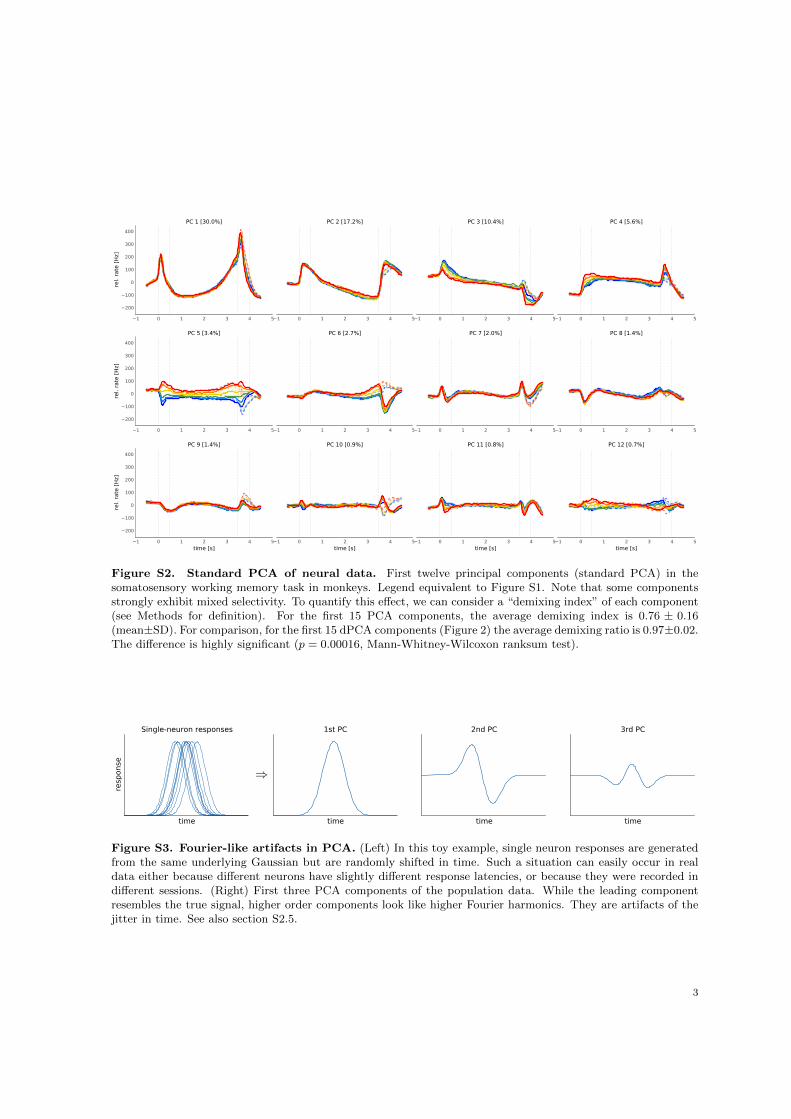
1 0 1 2 3 4 5
200
100
0
100
200
300
400
rel. r
ate
[H
z]
PC 1 [30.0%]
1 0 1 2 3 4 5
PC 2 [17.2%]
1 0 1 2 3 4 5
PC 3 [10.4%]
1 0 1 2 3 4 5
PC 4 [5.6%]
1 0 1 2 3 4 5
200
100
0
100
200
300
400
rel. r
ate
[H
z]
PC 5 [3.4%]
1 0 1 2 3 4 5
PC 6 [2.7%]
1 0 1 2 3 4 5
PC 7 [2.0%]
1 0 1 2 3 4 5
PC 8 [1.4%]
1 0 1 2 3 4 5
time [s]
200
100
0
100
200
300
400
rel. r
ate
[H
z]
PC 9 [1.4%]
1 0 1 2 3 4 5
time [s]
PC 10 [0.9%]
1 0 1 2 3 4 5
time [s]
PC 11 [0.8%]
1 0 1 2 3 4 5
time [s]
PC 12 [0.7%]
Figure S2. Standard PCA of neural data. First twelve principal components (standard PCA) in thesomatosensory working memory task in monkeys. Legend equivalent to Figure S1. Note that some componentsstrongly exhibit mixed selectivity. To quantify this effect, we can consider a “demixing index” of each component(see Methods for definition). For the first 15 PCA components, the average demixing index is 0.76 ± 0.16(mean±SD). For comparison, for the first 15 dPCA components (Figure 2) the average demixing ratio is 0.97±0.02.The difference is highly significant (p = 0.00016, Mann-Whitney-Wilcoxon ranksum test).
time
resp
onse
⇒
Single-neuron responses
time
1st PC
time
2nd PC
time
3rd PC
Figure S3. Fourier-like artifacts in PCA. (Left) In this toy example, single neuron responses are generatedfrom the same underlying Gaussian but are randomly shifted in time. Such a situation can easily occur in realdata either because different neurons have slightly different response latencies, or because they were recorded indifferent sessions. (Right) First three PCA components of the population data. While the leading componentresembles the true signal, higher order components look like higher Fourier harmonics. They are artifacts of thejitter in time. See also section S2.5.
3
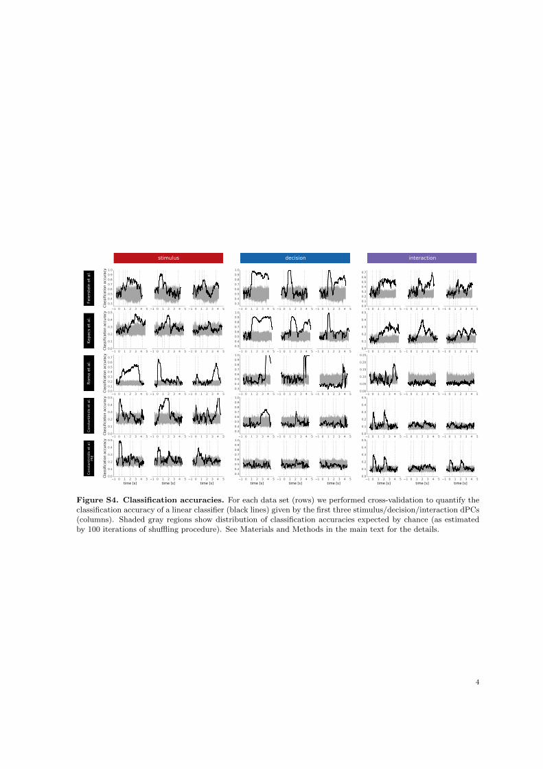
1 0 1 2 3 4 5
0.3
0.4
0.5
0.6
0.7
0.8
0.9
1.0
Cla
ssific
ati
on a
ccura
cy
1 0 1 2 3 4 5 1 0 1 2 3 4 5 1 0 1 2 3 4 5
0.3
0.4
0.5
0.6
0.7
0.8
0.9
1.0
1 0 1 2 3 4 5 1 0 1 2 3 4 5 1 0 1 2 3 4 50.0
0.1
0.2
0.3
0.4
0.5
0.6
0.7
1 0 1 2 3 4 5 1 0 1 2 3 4 5
Feie
rste
in e
t al.
1 0 1 2 3 4 50.0
0.1
0.2
0.3
0.4
0.5
Cla
ssific
ati
on a
ccura
cy
1 0 1 2 3 4 5 1 0 1 2 3 4 5 1 0 1 2 3 4 5
0.3
0.4
0.5
0.6
0.7
0.8
0.9
1.0
1 0 1 2 3 4 5 1 0 1 2 3 4 5 1 0 1 2 3 4 50.0
0.1
0.2
0.3
0.4
0.5
1 0 1 2 3 4 5 1 0 1 2 3 4 5
Kepecs
et
al.
1 0 1 2 3 4 50.0
0.1
0.2
0.3
0.4
0.5
0.6
0.7
Cla
ssific
ati
on a
ccura
cy
1 0 1 2 3 4 5 1 0 1 2 3 4 5 1 0 1 2 3 4 5
0.3
0.4
0.5
0.6
0.7
0.8
0.9
1.0
1 0 1 2 3 4 5 1 0 1 2 3 4 5 1 0 1 2 3 4 50.00
0.05
0.10
0.15
0.20
0.25
1 0 1 2 3 4 5 1 0 1 2 3 4 5
Rom
o e
t al.
1 0 1 2 3 4 50.0
0.1
0.2
0.3
0.4
0.5
Cla
ssific
ati
on a
ccura
cy
1 0 1 2 3 4 5 1 0 1 2 3 4 5 1 0 1 2 3 4 5
0.3
0.4
0.5
0.6
0.7
0.8
0.9
1.0
1 0 1 2 3 4 5 1 0 1 2 3 4 5 1 0 1 2 3 4 50.0
0.1
0.2
0.3
0.4
0.5
1 0 1 2 3 4 5 1 0 1 2 3 4 5
Const
anti
nid
is e
t al.
1 0 1 2 3 4 5
time [s]
0.0
0.1
0.2
0.3
0.4
0.5
Cla
ssific
ati
on a
ccura
cy
1 0 1 2 3 4 5
time [s]1 0 1 2 3 4 5
time [s]1 0 1 2 3 4 5
time [s]
0.3
0.4
0.5
0.6
0.7
0.8
0.9
1.0
1 0 1 2 3 4 5
time [s]1 0 1 2 3 4 5
time [s]1 0 1 2 3 4 5
time [s]
0.0
0.1
0.2
0.3
0.4
0.5
1 0 1 2 3 4 5
time [s]1 0 1 2 3 4 5
time [s]
Const
anti
nid
is e
t al.
PR
E
stimulus decision interaction
Figure S4. Classification accuracies. For each data set (rows) we performed cross-validation to quantify theclassification accuracy of a linear classifier (black lines) given by the first three stimulus/decision/interaction dPCs(columns). Shaded gray regions show distribution of classification accuracies expected by chance (as estimatedby 100 iterations of shuffling procedure). See Materials and Methods in the main text for the details.
4
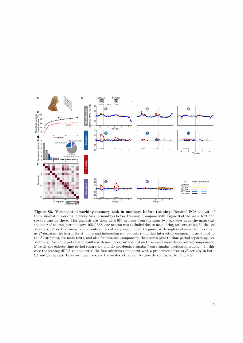
0 1 2 3 4−100
−50
0
50
100
Time (s)
0 1 2 3 4−60
−40
−20
0
20
40
60
Time (s)0 1 2 3 4
Time (s)
20
40
60
80
1 5 10 150
2
4
6
8
10
Com
pone
nt v
aria
nce
(%)
1 5 10 15Component
Cum
ulat
ive
expl
aine
dsi
gnal
var
ianc
e (%
)
Component
Com
pone
nt
1 5 10 15
1
5
10
15
−1 −0.5 0 0.5 1
a
c
d
e
b
Stimulus: 25%
Condition-independent: 64%
Interaction: 11%
Nor
mal
ized
firi
ng r
ate
(Hz)
Condition-ind.
Stimulus
Decision
Interaction
0 1 2 3 4Time (s)
1 2 4
3 9 11
5 10preferred45° away90° away
135° awayopposite
match non-matchF1
Stimulus Stimulus
0.5 s 1.5 s 0.5 s
S1 S2+
PCA
dPCA
−100
−50
0
50
100
100
Figure S5. Visuospatial working memory task in monkeys before training. Demixed PCA analysis ofthe visuospatial working memory task in monkeys before training. Compare with Figure 3 of the main text andsee the caption there. This analysis was done with 673 neurons from the same two monkeys as in the main text(number of neurons per monkey: 105 / 568; one neuron was excluded due to mean firing rate exceeding 50 Hz, seeMethods). Note that many components come out very much non-orthogonal, with angles between them as smallas 27 degrees: this is true for stimulus and interaction components (note that interaction components are tuned tothe S2 stimulus, see main text), and also for stimulus components themselves (due to time period separating, seeMethods). We could get clearer results, with much more orthogonal and also much more de-correlated components,if we do not enforce time period separation and do not demix stimulus from stimulus-decision interaction. In thiscase the leading dPCA component is the first stimulus component with a pronounced “sensory” activity in bothS1 and S2 periods. However, here we show the analysis that can be directly compared to Figure 3.
5

−100
−50
0
50
100
−20
−10
0
10
20
−50
0
50
−60
−40
−20
0
20
40
60
20
40
60
80
100
25
−25
1 5 10 150
2
4
6
8
10
Com
pone
nt v
aria
nce
(%)
1 5 10 15Component
Cum
ulat
ive
expl
aine
dsi
gnal
var
ianc
e (%
)
Component
Com
pone
nt
1 5 10 15
1
5
10
15
−1 −0.5 0 0.5 1
a
c
d
e
b
Nor
mal
ized
firi
ng r
ate
(Hz)
Condition-ind.
Stimulus
Decision
Interaction
Odour port Reward port
Stimulus: 2%Decision: 8%
Condition-independent: 82%
Interaction: 8%
PCA
dPCA
31 17RightLeft
Rightchoice
Leftchoice
Odour
Odourport
Rightchoice
Leftchoice
1
2 3
19 20
6 8 15
5 11 13
Dot productsbetween axes
Correlationsbetween
components
CH3CH3H3C
O
11
Anticipation
period
0 1 2 3 4Time (s)
5 0 1 2 3 4Time (s)
5 0 1 2 3 4Time (s)
5
0 1 2 3 4Time (s)
5
rewarded
conditions
Figure S6. dPCA of olfactory discrimination task in rats without re-stretching Here, using data fromthe olfactory discrimination task in rats, we demonstrate that applying dPCA to the non-re-stretched data leadsto qualitatively the same results as applying it to the re-stretched data as was done in the main text, see Figure4. The purpose of re-stretching was to average over trials while aligning on five events of interest: odour portenter, odour port exit, reward port enter, reward delivery, and reward port exit (see Methods). Here we averageover trials by cutting out a ±450 ms time interval around each event of interest and concatenating these cutstogether (so that each trial results in a 450 · 2 · 5 = 4500 ms long “piecewise” PSTH). Then we apply the samedPCA procedure (the optimal value of regularization parameter λ for these data, when normalized by the totalvariance, was 1.3 ·10−5, close to that for the re-stretched data). See Figure 4 in the main text for the full caption.Vertical gray lines on all subplots in (b) show alignment events, as on Figure 4. Dashed black lines show timepoints of cuts, e.g. mark discontinueties in time.
6
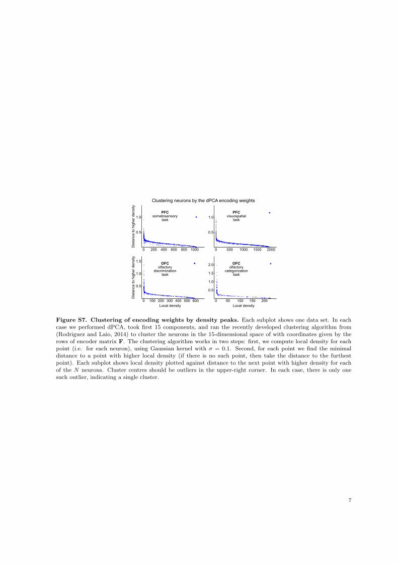
0 100 200 300 400 500 600
0.5
1.0
1.5
Local density
Dis
tanc
e to
hig
her
den
sity
0 50 100 150 200
0.5
1.0
1.5
2.0
0 200 400 600 800 1000
0.5
1.0
0 500 1000 1500 2000
0.5
1.0
Clustering neurons by the dPCA encoding weights
Local density
Dis
tanc
e to
hig
her
den
sity
PFCsomatosensory
task
PFCvisuospatial
task
OFColfactory
discriminationtask
OFColfactory
categorizationtask
Figure S7. Clustering of encoding weights by density peaks. Each subplot shows one data set. In eachcase we performed dPCA, took first 15 components, and ran the recently developed clustering algorithm from(Rodriguez and Laio, 2014) to cluster the neurons in the 15-dimensional space of with coordinates given by therows of encoder matrix F. The clustering algorithm works in two steps: first, we compute local density for eachpoint (i.e. for each neuron), using Gaussian kernel with σ = 0.1. Second, for each point we find the minimaldistance to a point with higher local density (if there is no such point, then take the distance to the furthestpoint). Each subplot shows local density plotted against distance to the next point with higher density for eachof the N neurons. Cluster centres should be outliers in the upper-right corner. In each case, there is only onesuch outlier, indicating a single cluster.
7

1 2 3 4 5 6 7 8 9126500
126000
125500
125000
124500
124000
123500Bayesian Information Criterion
0 2 4 6 8 10200
0
200
400
600
800
1000# neurons in each cluster (diag)
10 5 0 5 10 15 200
50
100
150
200
250First two clusters
15 10 5 0 5 10 15 20 2540
20
0
20
40
60
80First three clusters
30 20 10 0 10 20 30 40 50 6030
20
10
0
10
20
30
40
50First four clusters
1 2 3 4 5 6 7 8 925000
24500
24000
23500
23000
22500
22000
21500
21000
0 2 4 6 8 1050
0
50
100
150
200
250
30 25 20 15 10 5 0 50
20
40
60
80
100
120
5 4 3 2 1 0 1 2 3 425
20
15
10
5
0
5
10
15
20 15 10 5 0 5 10 15141210
8642024
1 2 3 4 5 6 7 8 962000
61000
60000
59000
58000
57000
56000
55000
0 2 4 6 8 10100
0
100
200
300
400
500
10 5 0 5 10 150
20
40
60
80
100
120
140
40 20 0 20 40 6064202468
1012
4 3 2 1 0 1 2200
0
200
400
600
800
1000
1 2 3 4 5 6 7 8 9188000
186000
184000
182000
180000
178000
176000
174000
0 2 4 6 8 10200
0
200
400
600
800
1000
1200
20 10 0 10 20 30 400
100
200
300
400
500
600
20 10 0 10 20 30 4040200
20406080
100120140
100 50 0 50 100 150 2005
4
3
2
1
0
1
2
1 2 3 4 5 6 7 8 9158000
156000
154000
152000
150000
148000
146000
0 2 4 6 8 10200
0
200
400
600
800
1000
1200
4 3 2 1 0 1 20
50
100
150
200
250
300
350
15 10 5 0 5 10 15 20 2540
20
0
20
40
60
80
100
120
15 10 5 0 5 10 15 20 25 306040200
20406080
100120
Rom
o e
t al.
Kepecs
et
al.
Feie
rste
in e
t al.
Const
anti
nid
is e
t al.
PR
EC
onst
anti
nid
is e
t al.
PO
ST
Figure S8. Clustering of encoding weights with Gaussian Mixture Models. Each row shows one dataset. In each case we performed dPCA, took 10 components in each marginalization (40 columns in total), andattempted to cluster N points (one for each neuron) in the 40-dimensional space with coordinates given by therows of encoder matrix F. We fitted Gaussian Mixture Model (GMM) with K Gaussians and diagonal covariancematrices Σk. First column: Bayesian Information Criterion (BIC) as a function of the number of clusters. In eachcase BIC indicated that 2–3 clusters provide the optimal fit to the data. We argue, however, that this outcomeis misleading in the sense that there are no separate clusters at all (so the optimal K is in fact equal to 1), seebelow. Second column: the number of neurons per cluster (red dots denote clusters with only a single neuron).Third column: we fitted GMM with two clusters, projected the data on the subspace with strongest separation oftwo clusters (obtained using linear discriminant analysis, LDA), and show distributions of values in each cluster.Note that “clusters” are hardly separated. Fourth and fifth column: equivalent to the third column but for GMMfitted with three and four clusters respectively, and data projected onto two-dimensional LDA subspace. Noteagain that the clusters are hardly separated; instead there is one cloud of points that is not perfectly Gaussianand so GMM chooses to fit it with several “clusters”.
8
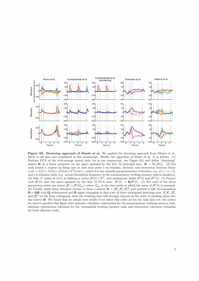
−200
0
200
Romo et al.
Stim
ulus
−200
0
200
Dec
isio
n
0 1 2 3 4
−200
0
200
Inte
ract
ion
−200
−100
0
100
200
Constantinidis et al.
−200
−100
0
100
200
0 1 2 3 4−200
−100
0
100
200
−200
−100
0
100
200
Constantinidis et al.pre-training
−200
−100
0
100
200
0 1 2 3 4−200
−100
0
100
200
−100
−50
0
50
100
Feierstein et al.
−100
−50
0
50
100
0 1 2 3 4−100
−50
0
50
100
−100
−50
0
50
100
Kepecs et al.
−100
−50
0
50
100
0 1 2 3 4−100
−50
0
50
100
Nor
mal
ized
firin
g ra
te (
Hz)
Time (s) Time (s) Time (s) Time (s) Time (s)
Figure S9. Demixing approach of Mante et al. We applied the demixing approach from (Mante et al.,2013) to all data sets considered in this manuscript. Briefly, the algorithm of Mante et al. is as follows. (1)Perform PCA of the trial-average neural data (as in our manuscript, see Figure S2) and define “denoising”matrix K as a linear projector on the space spanned by the first 12 principal axes: K = U12U
>12. (2) For
each neuron i, regress its firing rate at each time point t on stimulus, decision, and interaction between them:xi(t) = βoi (t)+βsi (t)s+βdi (t)d+βsdi (t)sd+ε, where d is any suitable parametrization of decision, e.g. d ∈ [−1,+1],and s is stimulus value (e.g. actual stimulation frequency in the somatosensory working memory task in monkeys).(3) Take N values of βsi (t) as defining a vector βs(t) ∈ RN , and analogously define βd(t) and βsd(t). (4) Projecteach βφ(t) onto the space spanned by the first 12 PCA axes: βφ(t) → Kβφ(t). (5) For each of the threeparameters select one vector βφ∗ = βφ(tφmax) where tφmax is the time point at which the norm of βφ(t) is maximal.(6) Finally, stack three obtained vectors to form a matrix B = [βs∗,β
d∗,β
sd∗ ] and perform a QR decomposition
B = QR with Q orthonormal and R upper triangular to find a set of three orthogonal demixing axes. If βs∗, βd∗,
and βsd∗ are far from orthogonal, then the resulting axes will strongly depend on the order of stacking them intothe matrix B. We found that we obtain best results if we select this order ad hoc for each data set; the orderswe used to produce this figure were stimulus→decision→interaction for the somatosensory working memory task,stimulus→interaction→decision for the visuospatial working memory task, and interaction→decision→stimulusfor both olfactory tasks.
9

Firi
ng
rate
(H
z)
0 Time (s)
Firi
ng
rate
(H
z)
Trial 1
Trial 2
Firi
ng
rate
(H
z)
0 Time (s)
Firi
ng
rate
(H
z)
Raw firing rates Restretched firing rates
⇨
⇨
alignment events
t2 t3t1=0 T2 T3T1=0
median alignment events
Figure S10. Restretching procedure. When analyzing the self-paced olfactory datasets, we used the followingre-stretching procedure to equalize the length of all trials and to align several events of interest. We defined severalalignment events (such as odour poke in, odour poke out, etc.) and for each trial found the times ti of theseevents. After aligning all trials on t1 = 0 (left) we computed median times Ti for all other events. Then foreach trial the firing rate we re-stretched on each interval [ti, ti+1] to align it with [Ti, Ti+1] (right). After suchrestretching, all events are aligned and the trials corresponding to one condition can be averaged.
0 1 2 3 4
−200
20406080
100
Firi
ng
rate
(H
z)
Time (s)
−200
20406080
100
Firi
ng
rate
(H
z)
−200
20406080
100
Firi
ng
rate
(H
z)
Mean firing rate
=
Condition-independent
++
Stimulus Decision
+
Interaction
+
++++=
++++=
Figure S11. Marginalization procedure. PSTHs of three exemplary neurons from the somatosensory workingmemory task decomposed into marginalizations. See section S2.1 for details.
10

0 1 2 3 4
−100
−50
0
50
100
Time (s)
Nor
mal
ized
firin
g ra
te (
Hz)
First four stimulus components without enforced time period separation
2.8%
1.3% 0.5%0.5%
First four stimulus components with enforced time period separation
−100
−50
0
50
100
Nor
mal
ized
firin
g ra
te (
Hz)
0 1 2 3 4Time (s)
0 1 2 3 4Time (s)
0 1 2 3 4Time (s)
0 1 2 3 4Time (s)
0 1 2 3 4Time (s)
0 1 2 3 4Time (s)
0.2%
0.4% 0.3% 0.2%
56° 50°
74°90°
83°
Figure S12. Time period separation in dPCA. On the top: first four stimulus components in the so-matosensory working memory task, as obtained with dPCA without time period separation. On the bottom: firstfour stimulus components in the same dataset, with the additional time period separation constraint (see Methodsfor description). Components on the bottom are identical to the ones shown on Figure 2. The encoding axes forthe components on the top are all mutually orthogonal, because they come from the same marginalization (seeMethods), the stimulus one. However, the encoding axes for the components in the bottom are far from beingorthogonal (angles are shown for various pairs of components). This is because now the algorithm effectively splitsstimulus marginalization into three different ones (see Methods), corresponding to the three pre-defined time pe-riods. Components shown here are arranged according to these time periods: first component has most of thevariance in the S1 period, second and fourth — in the delay period, third – in the S2 period. Notice that the twocomponents describing the delay period are exactly orthogonal, by construction. Proportion of variance of eachprojection is shown in each subplot in bold. It might seem that the components below account for substantiallyless variance than the components on the top, however the amount of explained variance (see Methods) by thefirst four components is very similar in both cases: 5.8% (top) and 5.4% (bottom).
11

0 1 2 3 4
100
50
0
50
100
rel. r
ate
[H
z]
0 1 2 3 4
0 1 2 3 460
40
20
0
20
40
60
rel. r
ate
[H
z]
0 1 2 3 4
0 1 2 3 460
40
20
0
20
40
60
rel. r
ate
[H
z]
0 1 2 3 4
0 1 2 3 4
time [s]
60
40
20
0
20
40
60
rel. r
ate
[H
z]
0 1 2 3 4
time [s]
0 1 2 3 4 0 1 2 3 4
0 1 2 3 4 0 1 2 3 4
0 1 2 3 4 0 1 2 3 4
0 1 2 3 4
time [s]0 1 2 3 4
time [s]
Regularized dPCs Unregularized dPCs
tim
edeci
sion
stim
ulu
sin
tera
ctio
n
Figure S13. Overfitting in dPCA. Demixed principal components in the olfactory discrimination task inrats without re-stretching (two in each marginalization) in the standard regularized case (left) and withoutregularization, λ = 0 (right). The cross-validation error for un-regularized case is large, see Figure S14. Seealso section S2.3 for more details. The components on the left are the same ones presented in the main text inFigure 4.
12

10-7 10-6 10-5 10-40.2
0.4
0.6
0.8
1.0
1.2
Rela
tive r
esi
dual vari
ance
on t
est
data
Relative cross-validation error over all marginalizations
Feierstein et al.Romo et al.Constantinidis et al. (POST)Kepecs et al.Constantinidis et al. (PRE)
10-7 10-6 10-5 10-40.2
0.4
0.6
0.8
1.0
1.2Feierstein et al.
10-7 10-6 10-5 10-40.2
0.4
0.6
0.8
1.0
1.2Romo et al.
10-7 10-6 10-5 10-40.2
0.4
0.6
0.8
1.0
1.2Constantinidis et al. (POST)
10-7 10-6 10-5 10-4
Regularization parameter lambda [1e-7]
0.2
0.4
0.6
0.8
1.0
1.2Kepecs et al.
10-7 10-6 10-5 10-4
Regularization parameter lambda [1e-7]
0.2
0.4
0.6
0.8
1.0
1.2Constantinidis et al. (PRE)
condition-independentdecisionstimulusinteraction
Figure S14. Cross-validation errors depending on the regularization parameter λ. Top left: mean(solid lines) and min/max (boundaries of shaded regions) of the relative cross-validation errors over all marginal-izations for 10 repetitions. Different colors refer to different datasets, the minimum is marked by a dot. Othersubplots: the same for each dataset, with different marginalizations showed separately. In each dataset the mini-mum cross-validation error is roughly the same across marginalizations, therefore we chose to use the same valueof λ in all marginalizations. See also section S2.3 for more details.
13
S2 Supplementary notes
S2.1 Marginalized averages
S2.1.1 Intuition
In order to identify components that depend onlyon a small number of parameters, it is necessary torigorously quantify the dependence of a componenton the set of parameters or labels. For illustra-tive purposes, consider a function x(t, s) that de-pends on time t (ranging from 1 to T) and stimuluss (ranging from 1 to S), Figure S15. We aim tosegregate this function into contributions that aresolely due to variations in either time or stimulusand contributions that are due to interactions ofboth parameters,
x(t, s) = µ+ z(t) + z(s) + z(t, s). (1)
There are many ways to perform this segregation.We pose, however, that the scalar µ should be the“best guess” about the value of x(t, s) if neithertime nor stimulus are determined. In other words,µ should simply be the mean of x,
µ =1
TS
∑
t,s
x(t, s) = 〈x(t, s)〉t,s (2)
where 〈.〉 denotes the average over all subscriptedparameters. The time-dependent term z(t), on theother hand, should be the best estimate of the re-mainder x(t, s)−µ if the stimulus is undetermined.For a given time-point t this is again just the aver-age over all undetermined parameters,
z(t) = 〈x(t, s)− µ〉s . (3)
A similar reasoning applies to the stimulus compo-nent,
z(s) = 〈x(t, s)− µ〉t . (4)
Finally, the interaction component z(t, s) is simplythe remainder,
z(t, s) = x(t, s)− µ− z(t)− z(s). (5)
We call each term of this specific segregation amarginalized average and note a range of useful pro-prerties: (1) Most trivially, the segregation is com-plete, i.e. we don’t loose any information about the
original function. (2) Averaging any marginalizedaverage over one of its parameters gives zero, i.e.
〈z(t)〉t = 0, 〈z(s)〉s = 0, (6)
〈z(t, s)〉t = 0, 〈z(t, s)〉s = 0. (7)
This property is useful to see that, (3), the differentterms are independent, i.e their covariance is zero,e.g.
〈z(t)z(s)〉t,s = 0 (8)
or〈z(t)z(t, s)〉t,s = 0. (9)
In this case the variance of x(t, s) can be written asthe sum of the marginalized variance,
Var(x(t, s)) = Var(z(t)) + Var(z(s)) + Var(z(t, s)).(10)
This property finally allows a well-grounded state-ment on how the variance of x(t, s) can be at-tributed to its parameters. We will make extensiveuse of this property when we define the objectivefor our demixing procedure. Before we generalizethe notion of marginalized averages to vector-valuedfunctions and more parameters, we clarify the rela-tionship to a well-known statistical method.
S2.1.2 Analysis of Variance
The marginalization procedure we introduced aboveturns out to be exactly equivalent to a linear modelwith categorical predictors used in ANOVA (analy-sis of variance) tests1.
ANOVA (in this case, two-way ANOVA) is oftenapplied as a statistical procedure to test whether afunction like x(t, s) varies with time, with stimulus,or with their interaction. In ANOVA terminology,time and stimulus are called factors and their indi-vidual values are called levels. If firing rate signifi-cantly varies with time, then we talk about signifi-cant main effect of time; the same goes for stimulus.If the effect of time is different for different stimu-lus values (or vice versa), then there is significantinteraction effect between time and stimulus.
Usually ANOVA is applied when there are mul-tiple measurements for each parameter combina-tion. In our case there is exactly one value for eachparameter combination (because we average overtrials as a pre-processing step; this has to be done,
1See e.g. Christensen R, 2011, Plane answers to complex questions: the theory of linear models (Springer) or RutherfordA, 2001, Introducing ANOVA and ANCOVA: a GLM approach (Sage).
14

time
resp
onse
=
y(t,s)
time
+
z(t)
time
+
z(s)
time
z(t,s)
Figure S15. An illustrative segregation of a simple time- and stimulus-dependent function x(t, s) into functionsz(t), z(s), z(t, s)
because different neurons come from different ses-sions with different numbers of trials). In such acase ANOVA would have no or very little power totest for statistical significance of individual effects,but the underlying linear model still makes senseand is equivalent to our marginalization procedure,as we show below.
To formulate the linear model, we introduce cat-egorical (dummy) variables xτ , xσ and xτσ,
xτ =
{1, if t = τ
0, otherwise.(11)
xσ =
{1, if s = σ
0, otherwise.(12)
xτσ =
{1, if t = τ and s = σ
0, otherwise.(13)
and consider the regression problem
x(t, s) = µ+∑
τ
zτxτ+∑
σ
zσxσ+∑
τ,σ
zτσxτσ. (14)
This regression problem is under-determined sincethere are more unknown parameters (1+T+S+TS)than data points (TS). A standard set of con-straints is therefore introduced in ANOVA as fol-lows:
∑
τ
zτ = 0, (15)
∑
σ
zσ = 0, (16)
∀τ :∑
σ
zτσ = 0, (17)
∀σ :∑
τ
zτσ = 0. (18)
The solution to this regression problem is ex-actly equivalent to the marginalized averages zτ ≡
x(τ), zσ ≡ x(σ) and zτσ ≡ x(τ, σ), see section S2.6,lemma 6.
S2.1.3 Generalization
We seek to generalize the definition of marginal-ized averages along two lines: first, to more thanone dependent variable and second, to more thantwo parameters. The first generalization is straight-forward: We apply the marginalization procedureto every single dependent variable. This amountsto replacing all scalar variables in (1-5) with vector-valued quantities.
To generalize the procedure to more than twoparameters we need to introduce a slightly morecumbersome notation. Instead of explicitly refer-encing every parameter (like time and stimulus), weonly reference the set of parameters S. In the two-parameter case above, the set would be S = {t, s}.More generally, the number of parameters is |S| andf(S) denotes a function that depends on all param-eters in S. Similarly, a function f(φ) depends onlyon a subset φ ⊆ S of parameters. This notationmakes it possible to generalize the splitting (1) as
x(S) =∑
φ⊆Sz(φ) (19)
where the sum goes over all possible subsets of pa-rameters in S. In the two-parameter case the setof subsets is given by {∅, {t} , {s} , {t, s}} and weequated z(∅) with the mean µ of the data. Thecorresponding marginalized averages are,
x(φ) = 〈x(S)〉S\φ −∑
τ⊂φx(τ), (20)
where 〈x(S)〉S\φ denotes the averaging of x(S) overall parameters y ∈ S that are not also elements ofy /∈ φ.
15

We already noted a range of useful properties ofmarginalized averages, all of which have a straight-forward generalization (see section S2.6 for proofs):
1. The average of x(φ) over any parameter y ∈ φis zero:
〈x(φ)〉y = 0 for y ∈ φ. (21)
In other words, it is not possible to split themarginalized averages z(φ) into a sum of func-tions with reduced parameter dependence inany meaningful way.
2. They are independent, i.e. their covariance iszero:
〈x(φ)x(φ′)〉S = 0. (22)
This, in turn, allows to segregate the datacovariance matrix C =
⟨x(S)x(S)>
⟩S
intoa sum of marginalized covariances Cφ =⟨x(φ)x(φ)>
⟩S
,
C =∑
φ
Cφ. (23)
3. There is an explicit formula for marginalizedaverages that does not rely on the hierarchicalcomputation from small to larger numbers ofparameters (i.e. is independent of the orderof evaluation),
x(φ) =∑
τ⊆φ(−1)|τ | 〈x〉(S/φ)∪τ . (24)
S2.2 dPCA optimization
Let X be a multidimensional data-matrix such thatthe first index refers to the observable (e.g. cellidentity) whereas all subsequent indices refer to dif-ferent parameters. As an example, Xnts refers tothe mean response of neuron n at time t and s. Formatrix products Z = UX we use the usual general-ization,
Zkts =∑
n
UknXnts. (25)
Similarly for the L2-norm,
‖X‖22 =∑
n,t,s
X2nts. (26)
Note that for algorithmic implementations it isstraight-forward to simply collapse all but the first
coordinate into one axis, thereby embedding themulti-dimensional data-matrix into the standardtwo-dimensional matrix space.
The marginalized data is denoted by Xφ. Notethat we assume that Xφ has the same shape as theoriginal data; parameters that have been averagedout during the marginalization are inserted back asreplications (e.g. Xt varies only along the temporalaxis but is constant in stimulus).
We can now define the objective for dPCA as amatrix equation,
LdPCA =∑
φ⊆S‖Xφ − FφDφX‖22 . (27)
The objective is defined such that we project thefull data X by means of Dφ (the decoder) on a low-dimensional latent space (the dPCs) and then aimto reconstruct the marginalized data by means of aprojection matrix Fφ (the encoder). In this way wefavour variance in a specified marginalization φ andpunish variance from other marginalizations.
Note that we do not necessarily sum over allmarginalizations but instead often pool marginal-izations that cannot be independent. As an ex-ample, consider a behavioural parameter like de-cision that usually carries variance only at the endof a trial. Inevitably, there is no way that decisioncan be independent of time and so we add decisionand decision-time together and consider them one“marginalization” (Xd + Xtd → Xtd).
One might be worried that the dPCA objective(27) is too biased towards demixed directions andmight neglect directions with mixed variance even ifthese directions carry high amounts of variance. Forthis reason it is tempting to trade demixing againstthe total explained variance of the data,
∥∥∥∥∥∥X−
∑
φ
FφDφX
∥∥∥∥∥∥
2
2
. (28)
It turns out, however, that in all neural datasetswe analysed we never found that demixing aloneleads to a strong decrease of the explained variance.Hence, all the data analysis in the subsequent sec-tions will be based on dPCA objective (27) alone.
Minimizing objective (27) is straight-forward.
16
Replacing Mφ = FφDφ we can rewrite (27) as
Mφ = arg minM
‖Xφ −MX‖22 ,
s.t. r(M) ≤ sφ.(29)
where r(M) is the rank of M and sφ is the numberof components desired in marginalization φ. With-out a rank constraint the solution to this regressionproblem is simply given by M∗
φ = XφX+ where X+
denotes the pseudo-inverse. The rank-constrainedproblem (“reduced rank regression”) is then solvedby those sφ projections that carry the most variance(see Reinsel et al. 1998 or Izenman 1975), i.e.
Mφ = UφU>φM∗
φ = UφU>φXφX
+ (30)
where Uφ are the first sφ left singular vectors ofM∗
φX. Correspondingly, the encoder Fφ = Uφ isgiven by the left singular vectors whereas the de-coder is given by Dφ = U>φXφX
+.
S2.3 Regularization
Unfortunately, without any further constraints werun into serious over-fitting problems, see FigureS13. More precisely, if the number of neurons ison the same order as the number of independentdata points (which is true for all datasets analysedhere), then the distribution of eigenvalues of thedata covariance matrix will peak at zero. In high-dimensional spaces, the space of eigenvectors withvery small eigenvalues (the “kernel”) will likely par-tially overlap with the leading PCs in individualmarginalizations.
Without regularization, the decoder directionswill end up lying within the kernel such thatthey overlap with the leading PC directions inone marginalization but are orthogonal to all othersources of variance. These directions will have verysmall variance, and the norms of decoder columnswill be very large to compensate for that. Withonly slight instabilities of the kernel subspace, how-ever, the same decoder will strongly amplify noiseon a validation set, thereby leading to large cross-validation errors (see Figure S14).
A common approach to avoid such overfittingis to add a suitable regularization term. As we ex-plained above, strong overfitting results in the largeL2-norm of the decoder. For that reason we add a
regularization term to (29),
Mφ = arg minM
‖Xφ −MX‖22 + λ ‖M‖22 , (31)
subject to r(M) ≤ sφ, where λ is a regularizationparameter. Note that ‖M‖ = ‖D‖, because
‖M‖2 = ‖FD‖ = Tr(FDD>F>) (32)
= Tr(F>FDD>) = Tr(DD>) (33)
= ‖D‖2 , (34)
where we used orthogonality of F.We can rewrite this optimization problem in a
more compact form that allows an analytic solu-tion. Let M ∈ RN×N . We then stack X with theN×N -dimensional identity matrix IN and Xφ withthe N × N -dimensional zero matrix 0N along thecolumn index. As an example, if Xφ ∈ RN×K , thenthe elements of the stacking are
[Xφ,0N ]ij =
{[Xφ]ij if j ≤ K,[0N ]i(j−K) else.
(35)
In this way we can rewrite the regularized objective(31) as
Mφ = arg minM
‖Xφ −MX‖22 + λ ‖M‖22 , (36)
= arg minM
‖[Xφ,0N ]−M[X, λIN ]‖22 . (37)
subject to r(M) ≤ sφ. This formulation adheres tothe same treatment as (29).
Cross-validation to select λ
We performed cross-validation in order to select theoptimal value of the regularization parameter λ. Toseparate the data into training and testing sets, weheld out one random trial for each neuron in eachcondition as a set of test “pseudo-trials” Xtest (asthe neurons were not recorded simultaneously, wedo not have recordings of all N neurons in any ac-tual trial). Remaining trials were averaged to forma training set Xtrain. Note that Xtest and Xtrain
have the same dimensions.We then performed dPCA on Xtrain for vari-
ous values of λ, selected 10 components in eachmarginalization (i.e. 40 components in total) to ob-tain F(λ) and D(λ), and computed reconstructionerror R(λ) for λ between 10−7·‖X‖2 and 10−3·‖X‖2(on a logarithmic grid). We repeated this procedure
17

10 times for different train-test splittings and aver-aged the resulting functions R(λ). In all cases theaverage function R(λ) had a clear minimum (FigureS13) that we selected as the optimal λ.
We used two approaches to compute R(λ). Thefirst approach uses Xtest to predict Xtrain:
R1(λ) =
∑φ ‖Xtrain,φ − FφDφXtest‖2
‖Xtrain‖2, (38)
where we wrote F(λ) and D(λ) as F and D forcompactness. This is a fraction of training-set vari-ance not explained by the test data. Note that itwould not make sense to change Xtest and Xtrain
places here: the decoder and encoder are fitted tothe training data, and should only be applied to thetest data for the purposes of cross-validation.
The second approach uses Xtest only. A naiveimplementation
∑φ ‖Xtest,φ − FφDφXtest‖2
‖Xtest‖2(39)
is incorrect: here we use Xtest both for predictionand for evaluating this prediction, which is inac-ceptable (even though in practice often leads to verysimilar results). An alternative method predicts onedimension (i.e. one neuron) of Xtest at a time, usingall other dimensions:∑φ
∑Nn=1 ‖[Xtest,φ]n − [Fφ[Dφ]−n[Xtest]−n]n ‖2
‖Xtest‖2,
where [·]n stands for n-th coordinate and [·]−n forall coordinates except of the n-th one. The innersum in this expression can be computed analyti-cally, resulting in
R2(λ) =∑φ ‖Xtest,φ − (FφDφ − diag{FφDφ}) Xtest‖2
‖Xtest‖2,
(40)
We verified that using R1(λ) and R2(λ) yieldedthe same optimal λ in our data sets.
S2.4 Relation to Linear Discrimi-nant Analysis
A common dimensionality reduction technique re-lated to dPCA is linear discriminant analysis
(LDA). In this section we will argue that while LDAcan be applied to neural data for the purposes ofdemixing, it is less suited than dPCA.
In the LDA ansatz, every data point y belongsto a class k ∈ {1, . . . ,K}. Data points within eachclass k have a mean (centroid) µk and covarianceΣk. LDA assumes that all classes have the samecovariance, estimated2 as ΣW =
∑k Σk/K and
called within-class covariance. On the other hand,the centroids of all classes form the between-classcovariance
ΣB =1
K
K∑
k=1
(µk − µ)(µk − µ)> (41)
where µ =∑k µk/K.
LDA aims at finding directions (discriminantaxes) maximizing between-class and minimizingwithin-class variances. For the case of one axis w,LDA maximizes the following function:
LLDA =w>ΣBw
w>ΣWw. (42)
The general LDA solution is to take eigenvectorsof Σ−1W ΣB as discriminant axes (they will gener-ally not be mutually orthogonal, but projections onthem will have zero correlation).
Note that LDA is a one-way technique: there isonly one parameter, or label, associated with eachdata point — namely, its class k. Also, LDA is tra-ditionally applied in situations with only few classesand a large number of data points in each class. Itis therefore neither straightforward, nor customaryto apply LDA to a neural data set as the ones con-sidered in this manuscript to find demixing projec-tions. Nevertheless, it is possible to do, using thesame marginalization approach developed here fordPCA.
Consider a data set with time t, stimulus sand decision d as labels of the data points (withtotal number of different labels being T , S, andQ respectively). To find discriminant axes asso-ciated with e.g. stimulus, we can split the datainto stimulus marginalization and everything else:X = Xst+X(rest). We can then treat all SQT datapoints as belonging to one of the ST classes (with
2Note that these formulas are given for the case when all classes have the same number of points; in case of non-balancedclasses one has to use weighted averages.
18

centroids Xst) and Q points in each class. Conse-quently, Cst can be taken as between-class covari-ance matrix and C−Cst as the within-class one.
For the case of e.g. the somatosensory workingmemory task (T = 501, S = 6, Q = 2) this wouldcorrespond to 3006 classes with 2 points per class.This is an unusual setting for LDA, but one cannevertheless proceed with applying LDA to find aset of discriminant axes. There is, however, by farnot enough data points to reliably estimate within-class covariance matrix in the N = 832-dimensionalspace, and as LDA requires inverting this covariancematrix, it will result in severe over-fitting. A stan-dard approach in such a case is to use regularizedLDA (rLDA) by replacing ΣW with a “shrinkage”estimator (1 − λ)ΣW + λI. We found that by us-ing this approach and fine-tuning the regularizationparameter λ, we can obtain components that aresimilar to the dPCA components (data not shown).
Indeed, the objective functions of dPCA andLDA (as introduced above) can be shown to be sim-ilar to each other. In the case of a single decoder dand encoder p the dPCA objective (27) becomes
∥∥∥Xφ − pd>X∥∥∥2
2=
∥∥∥∥∥Xφ − pd>∑
τ
Xτ
∥∥∥∥∥
2
2
(43)
= ‖Xφ‖22 − 2p>XφX>φ d +
∑
τ
d>XτX>τ d, (44)
= ‖Xφ‖22 + (d− 2p)>ΣBd + d>ΣWd, (45)
where we used that the covariance between differ-ent marginalizations is zero (section S2.6, lemma3) and we defined between- and within-class covari-ance matrices following the discussion above:
ΣB = XφX>φ , (46)
ΣW =∑
τ 6=φXτX
>τ . (47)
To first order the encoder is equivalent to the firstPC of ΣB while the decoder d ≈ p + w can besplit such that w ensures the orthogonality to othersources of variance. Then p>ΣBd ≈ d>ΣBd andthe dPCA objective function can be written as,
LdPCA ≈ d>ΣBd− d>ΣWd, (48)
which corresponds to the LDA objective functiongiven above (42) in that it aims at maximizingbetween-class and minimizing within-class variance.
Even though LDA approach as outlined abovecan result in components close to the ones foundby dPCA, we consider dPCA a more principledand systematic approach to the demixing problem.In particular, LDA looks only for decoding axes(discriminant axes) and ignores the encoding axes.Therefore, unlike dPCA, it does not aim at repre-senting the original data set, does not provide anyuseful measures of explained variance, etc.
There is a multi-way, or factorial, extension ofLDA known as MANOVA (multivariate ANOVA).In MANOVA, each data point is labeled with sev-eral parameters, i.e. all points are split into classesin several different ways. Whereas LDA is usu-ally understood as either a dimensionality reduc-tion or classification technique, MANOVA is usu-ally understood as a statistical test; however, theunderlying mathematics is very similar. To use thesame neural example, MANOVA asks if the neu-ral population activity differs with time, stimulus,decision, or some interactions between these param-eters (ANOVA asks exactly the same about a sin-gle neuron). To answer this question, MANOVAconsiders within-class covariance matrix ΣW as ashared covariance matrix of all the smallest sub-classes, e.g. groups of points with fixed time, stim-ulus, and decision values; it then proceeds to com-pute various between-class covariance matrices ΣB
for various parameters and to analyze Σ−1W ΣB in or-der to perform the statistical test (compare it withANOVA that looks at the ratio of between-class andwithin-class variances, B/W , as the statisic of inter-est). Note, however, that in all cases considered inthis manuscript the number of points with a given(t, s, d) combination is exactly 1, so MANOVA can-not be applied. And even if it could be applied, itwould not address the demixing: as we saw above,ΣW should be defined differently for that purpose.
S2.5 Fourier-like components fromtemporal variations
Consider the decision components in the somatosen-sory working memory task, Figure 2. Here the sec-ond and the third components are closely resem-bling the first and second temporal derivatives ofthe leading decision component. To illustrate whythese components are likely to be artifacts of the un-derlying sampling process, consider a highly simpli-
19

fied example in which a population of N neurons isencoding a one-dimensional bell-shaped signal z(t)in the population vector a, i.e the population re-sponse is given by x(t) = az(t). In this case thepopulation response lies in the one-dimensional sub-space spanned by a and covariance matrix has rankone:
C =∑
t
x(t)x>(t) = aa>∑
t
z(t)2. (49)
Now consider the case in which the neurons arenot recorded simultaneously but are pooled fromdifferent sessions. In behavioural experiments it isunavoidable that the onset of neural responses willvary by tenths or hundreds of milliseconds. Hence,the individual response yi(t) of neuron i will expe-rience a small time-shift τi:
xi(t) = aiz(t+ τi), (50)
see Figure S3 for an illustrative example with Gaus-sian tuning curves.
If τi is small we can do a Taylor expansionaround t:
yi(t) = aiz(t) + aiτiz′(t) +O(τ2i ). (51)
Note that for pedagogical purposes we neglecthigher-order corrections, but the extension isstraight-forward. Let τ be the vector of time-shiftsof the neurons and let b = a◦τ be the element-wisevector product of a and τ , i.e. [a◦τ ]i = aiτi. Thenthe population response can be written as
x(t) ≈ az(t) + bz′(t). (52)
Hence, the covariance matrix is approximately,
C ≈∑
t
aa>z2(t) + bb>z′2(t) (53)
where we assumed for simplicity that a ⊥ b. Inother words, time-shifts between observations willresult in additional PCA components that roughlyresemble the temporal derivatives of the sourcecomponent.
S2.6 Mathematical proofs
Lemma 1 (Completeness). The segregation of x(S)into the marginals x(φ) is complete, i.e.
x(S) =∑
φ⊆Sx(φ). (54)
The proof follows directly from the definition(20). In addition to being complete, the individualmarginalized averages are not linearly dependent inany parameter,
Lemma 2 (Linear parameter independence). Theaverage of x(φ) over any parameter x ∈ φ is zero,
〈x(φ)〉x = 0 for x ∈ φ. (55)
Proof. Proof by induction: For y ∈ S the averageover y is zero,
〈x(x)〉y = 〈x(S)〉S − µ = 0. (56)
Let (55) be shown for all φ ⊂ S with ‖φ‖ ≤ N .Then, for ‖φ‖ = N + 1 and y ∈ φ,
〈x(φ)〉y = 〈x(S)〉S\(φ\y) −∑
τ⊂φ〈x(τ)〉y , (57)
= 〈x(S)〉S\(φ\y) −∑
τ⊆(φ\y)x(τ) (58)
= 〈x(S)〉S\(φ\y) −∑
τ⊂(φ\y)x(τ)− x(φ \ y),
(59)
= 0. (60)
The last equation follows from the definition ofx(φ \ y).
From lemma 1 and lemma 2 we can directly de-rive the independence of two marginalized averages.
Lemma 3 (Independence). Different marginalizedaverages are independent, i.e.
〈x(φ)x(φ′)〉S = 0. (61)
Proof. W.l.o.g. let φ ≥ φ′. For ξ = φ/φ′ =∅ ⇒ φ = φ′ so there is nothing to show. Forξ = φ/φ′ 6= ∅ we use the linearity of the averageand property (55),
〈x(φ)x(φ′)〉S =⟨〈x(φ)x(φ′)〉ξ
⟩S/ξ
=⟨〈x(φ)〉ξ x(φ′)
⟩S/ξ
= 0.
20

From the last lemma, together with (54), we canobtain an identity for the sum of covariance matri-ces.
Lemma 4 (Covariance splitting). The covariancematrices of the marginalized averages sum up to thefull covariance matrix,
C =∑
φ⊆SCφ (62)
for Cφ =⟨x(φ)x>(φ)
⟩.
Finally, we introduce an equivalent definition ofthe marginalized averages that only relies on cer-tain averages of x and is independent of the orderof evaluation.
Lemma 5 (Reformulation). For a given functionx(S) the set of marginalized averages
x(φ) =∑
τ⊆φ(−1)|τ | 〈x〉(S/φ)∪τ . (63)
is equivalent to (20).
The proof of this lemma is not straight-forward.We first prove that any splitting with property (54)and (55) is unique.
Lemma 6. Any segregation {x(φ)|φ ⊆ S} of x(S)that obeys the properties (54) and (55) is unique.
Proof. Let there be two sets {x} 6= {x′} that obey(54) and (55). Then,
∑
φ⊆Sx(φ) =
∑
φ⊆Sx′(φ). (64)
Using (55) we can average over S/y with y ∈ S tofind
x(y) = x′(y). (65)
Averaging over S/ {y, z} leads to
x(y) + x(z) + x(y, z) = x′(y) + x′(z) + x′(y, z),(66)
⇔ x(y, z) = x′(y, z). (67)
More generally, averaging over S \ξ with ξ ⊆ S andy ∈ S \ ξ yields
∑
φ⊆S\ξx(φ) + x(φ ∪ {y}) =
∑
φ⊆S\ξx′(φ) + x′(φ ∪ {y}),
(68)
⇔ x(ξ ∪ {y}) = x′(ξ ∪ {y}), (69)
by induction. Hence, {x} = {x′}.
This lemma considerably simplifies the proof ofthe closed-form definition of the marginalized aver-ages, lemma 5.
Proof. According to lemma 6 we only need to showthat the marginalized averages (63) have the prop-erty (54) and (55). Regarding completeness, werewrite x(S),
x(S) =∑
φ⊆Sx(φ) (70)
=∑
φ⊆S
∑
τ⊆φ(−1)|τ | 〈x〉(S\φ)∪τ (71)
=∑
φ⊆S
∑
τ⊆φ(−1)|τ | 〈x〉(S\(φ/τ)) (72)
=∑
ξ⊆S
∑
τ⊆S\ξ(−1)|τ | 〈x〉(S\ξ) (73)
=∑
ξ⊆S〈x〉(S\ξ)
∑
τ⊆S\ξ(−1)|τ |
(74)
From the binomial theorem we can compute theweighted sum over subsets,
=∑
ξ⊆S〈x〉(S\ξ) (1− 1)|S\ξ| (75)
= x(S). (76)
To proof the linear parameter independence (55),note that, for any y ∈ φ, we can rewrite (63) as
x(φ) =∑
τ⊆φ/y(−1)|τ |
(〈x〉(S\(φ\τ)) − 〈x〉(S\(φ\τ))∪y
).
(77)Averaging over y cancels all terms on the right andhence 〈x(φ)〉y = 0.
21