Demand for Crash Insurance, Intermediary Constraints,

and Stock Return Predictability

Hui Chen Scott Joslin Sophie Ni∗

December 31, 2013

Abstract

The net amount of deep out-of-the-money (DOTM) S&P 500 put options that

public investors purchase (or equivalently, the amount that financial intermediaries

sell) in a month is a strong predictor of future market excess returns. A one-standard

deviation decrease in our public net buy-to-open measure (PNBO) is associated with

a 3.4% increase in the subsequent 3-month market excess return. The predictive

power of PNBO is especially strong during the 2008-09 financial crisis, and it cannot

be accounted for by a wide range of standard return predictors, nor by measures of

tail risks or funding constraints. Moreover, PNBO is contemporaneously negatively

related to the expensiveness of the DOTM puts. To explain these findings, we build

a dynamic general equilibrium model in which financial institutions play a key role

in sharing tail risks. The time variation in the financial institutions’ intermediation

capacity drives both the equilibrium demand for crash insurance and the market risk

premium. Our results suggest that trading activities in the crash insurance market

is informative about the degree of financial intermediary constraints.

∗Chen: MIT Sloan and NBER (huichen@mit.edu). Joslin: USC Marshall (sjoslin@usc.edu). Ni: HongKong University of Science and Technology (sophieni@ust.hk). We thank Tobias Adrian, Robert Battalio,David Bates, Bryan Kelly, Andrew Lo, Dmitriy Muravyev, Jun Pan, Steve Ross, Martin Schneider, KenSingleton, Hao Zhou, and seminar participants at USC, MIT Sloan, HKUST, Notre Dame, WashingtonUniversity in St. Louis, New York Fed, Boston Fed, AFA, the Consortium of Systemic Risk AnalyticsMeeting, CICF, SITE, and the OptionMetrics Research Conference for comments, and Ernest Liu forexcellent research assistance. We also thank Paul Stephens at CBOE, Gary Katz and Boris Ilyevsky atISE for providing information on the SPX and SPY option markets.

1 Introduction

Trading activities in the market of deep out-of-the-money put options on the S&P 500

index (DOTM SPX puts) is informative about the market risk premium and the degree of

financial intermediary constraints. We construct a measure of the net amount of DOTM

SPX puts that public investors acquire each month (henceforth referred to as PNBO),

which also reflects the net amount of the same options that broker-dealers and market

makers sell in that month. PNBO is negatively related to the expensiveness of the DOTM

puts relative to the at-the-money options. Moreover, PNBO predicts future market returns

negatively. A one-standard deviation drop in PNBO is associated with a 3.4% increase in

the subsequent 3-month stock market excess return. Over the whole sample, the R2 for

the predictability regression is 17.4%.

This predictive power of PNBO is distinct from that of the standard return predictors

in the literature, such as price-earnings ratio, dividend yield, consumption-wealth ratio,

variance risk premium, default spread, term spread, and tail risk measures. The inclusion

of PNBO also drives out measures of financial intermediary funding constraints such as the

TED spread and changes in broker-dealer leverage in a predictability regression. Moreover,

the predictive power of PNBO is time-varying and was particularly strong during the

recent financial crisis. When estimating the predictive regression with PNBO using a

5-year moving window, the R2 changes from less than 5% most of the time prior to 2006

to close to 50% during the crisis period.

While previous studies have documented that public investors are typically net buyers

of DOTM SPX puts during normal times, the net public purchase of DOTM SPX puts

turned significantly negative during the peak of the 2008-2009 financial crisis, suggesting

that the broker-dealers and market makers switched from net sellers into buyers of market

crash insurances. The SPX option volume data do not allow us to directly identify which

types of public investors (retail or institutional) were selling the DOTM puts during

the crisis. However, a comparison of the public investor trading activities in the market

for SPX vs. SPY options (the latter is an option on the SPDR S&P 500 ETF Trust

and has a significantly higher percentage of retail investors than SPX options), as well

1

a comparison between large and small public orders of SPX puts suggest that it is the

institutional investors (e.g., hedge funds) who were selling the DOTM puts to the financial

intermediaries.

To explain these empirical findings, we build a dynamic general equilibrium model of

the crash insurance market. Financial intermediaries (dealers) are net providers of such

insurance under normal conditions, which could be because they are better at managing

crash risk than the public investors, or because they are less concerned with crash risk due

to agency problems.1 Over time, the risk sharing capacity of the intermediaries changes

due to endogenous trading losses and exogenous shocks to the intermediation capacity.

We capture these features in reduced form by assuming that the financial intermediaries

are more optimistic about crash risk than public investors during normal times, and that

their aversion to crash risk changes over time due to exogenous intermediation shocks.

In the model, public investors’ equilibrium demand for crash insurance depends on the

level of crash risk in the economy, the wealth distribution between public investors and

the financial intermediary, and shocks to the intermediation capacity. As the probability

of market crash rises, all else equal, public investors’ demand for crash insurance tends to

rise. However, if the financial intermediaries’ risk sharing capacity drops at the same time

due to loss of wealth or increase in crash aversion, the equilibrium amount of risk sharing

can become smaller. Furthermore, because of reduced risk sharing, public investors now

demand a higher premium for bearing crash risk. This mechanism can generate significant

variation in market risk premium due to the high sensitivity of market risk premium to

the amount of risk sharing of tail risks as shown in Chen, Joslin, and Tran (2012).

Empirically, the market for deep out-of-the-money SPX puts closely resembles the crash

insurance market in our model for two reasons. First, while the financial intermediaries can

partially hedge the risks of their option inventories by trading futures and over-the-counter

(OTC) derivatives, the hedge is imperfect and costly. This is especially true for DOTM

puts, which are highly sensitive to jump risks that are more difficult to hedge. Thus, the

1Examples include government guarantees to large financial institutions and compensation schemesthat encourages managers to take on tail risk. See e.g., Lo (2001), Malliaris and Yan (2010), Makarov andPlantin (2011).

2

impact of intermediation capacity is likely to be more significant for these options. Second,

while DOTM index puts are not the only way to hedge against crash risks, compared to

OTC derivatives, SPX puts provide unique advantages in that the central counterparty

clearing and margin system largely removes the counterparty risks and enhances liquidity.

Our paper builds on and extends the work of Garleanu, Pedersen, and Poteshman

(2009) (henceforth GPP), who develop a partial equilibrium model demonstrating how

exogenous public demand shocks affect option prices when risk-averse dealers have to bear

the inventory risk. In their model, the dealers’ intermediation capacity is fixed, and the

model implies a positive relation between the public demand for options and the option

premium. Like GPP, the limited intermediation capacity of the dealers is a central feature

of our model, but we introduce shocks to the intermediation capacity and endogenize the

public demand for options, option pricing, and aggregate market risk premium jointly in

general equilibrium. In our model, the relation between the equilibrium demand for the

put options and the option premium can be either positive or negative.

Our paper contributes to the literature on the impact of financial intermediary con-

straints on asset pricing and the real economy. Recent theoretical contributions include

Gromb and Vayanos (2002), Brunnermeier and Pedersen (2009), Geanakoplos (2009), He

and Krishnamurhty (2012), Brunnermeier and Sannikov (2013), Gertler and Kiyotaki

(2013), among others. As shown in several of these models, the financing constraints

change the effective risk aversion of the intermediaries. Motivated by this insight, we

directly model intermediation shocks via dealers’ time-varying risk aversion towards crash

risks, which makes the model analytically tractable and easy to calibrate. Similar to

Adrian and Boyarchenko (2012), who explicitly model a risk-based capital constraint

for intermediaries, both the dealer net worth and leverage drive market prices of risk in

our model. We also provide new evidence consistent with the prediction of intermediary

constraints influencing the pricing of financial assets and the aggregate risk premium.

Different from earlier empirical studies by Adrian and Shin (2010), Adrian, Moench,

and Shin (2010), and Adrian, Etula, and Muir (2012), who use intermediary leverage to

measure the constraint, our measure is based on financial intermediaries’ options positions,

3

which has the advantage of being forward-looking and available at high (daily) frequency.

Pan and Poteshman (2006) show that option trading volume predicts near future

individual stock returns (up to 2 weeks). They find the source of this predictability to be

the nonpublic information possessed by option traders. In contrast, our evidence of return

predictability applies to a market index and to longer horizons (up to 4 months). Moreover,

we argue that the economic source of this predictability is time-varying intermediary

constraints. Hong and Yogo (2012) find that open interests in commodity futures are

pro-cyclical and predict commodity returns positively. Our measure of net public purchase

is different from open interest. If public investors only trade among themselves (e.g., due to

heterogeneous beliefs, risk aversion, or background risks), there will be large open interest

but zero net public purchase for options. Moreover, the return predictability we find for

net public purchase is negative, opposite to that of open interest in Hong and Yogo (2012).

Several studies have examined the role that the derivatives markets play in the aggregate

economy. Buraschi and Jiltsov (2006) study option pricing and trading volume when

investors have incomplete and heterogeneous information. Bates (2008) shows how options

can be used to complete the markets in the presence of crash risk. Longstaff and Wang

(2012) show that the credit market plays an important role in facilitating risk sharing

among heterogeneous investors. Chen, Joslin, and Tran (2012) show that the aggregate

market risk premium is highly sensitive to the amount of risk sharing of tail risks in

equilibrium.

2 Empirical Evidence

In this section, we present the empirical evidence connecting the trading activities of

deep out-of-the-money S&P 500 put options (DOTM SPX puts) between public investors

and financial intermediaries to the pricing of these options and the risk premium of the

aggregate stock market.

4

2.1 Data and variables

The data used to construct our option demand measures are from the Chicago Board

Options Exchange (CBOE). The Options Clearing Corporation classifies each option

trade into one of three categories based on who initiates the trade. They include public

investors (or customers), firm investors, and market makers. Transactions initiated by

public investors include those made by retail investors and those by institutional investors

such as hedge funds or mutual funds. Trades initiated by firm investors correspond to

those that the securities broker-dealers (who are not designated market makers) make

for their own accounts or for another broker-dealer. The SPX options volume data are

available at daily frequency from 1991 to 2012. Option pricing and open interest data are

obtained from the OptionMetrics for the period of 1996 to 2012.

Our main option volume variable is PNBO, which is defined as the total open-buy

orders of all the DOTM SPX puts (with strike-to-price ratio K/S ≤ 0.85) by public

investors minus their open-sell orders on the same set of options in each month. We

use the strike-to-price ratio to classify DOTM options because it is parsimonious and

model-independent. Later on we also present he results based on other strike-to-price

cutoffs as well as moneyness cutoffs that adjust for option maturity and recent volatility of

the S&P 500 index. We focus on open orders (orders to open new positions) because Pan

and Poteshman (2006) and others have shown that these orders can be more informative

than close orders. For comparison, we also consider the measure PNB, which is the public

investors’ net buying volume that includes both open and close orders.

Since options are in zero net supply, the amount of net buying by the public investors

is equal to the amount of net selling by the firm investors and market makers. Since

our focus is to connect option market trading activities to the constraints of financial

intermediaries, it is natural to group the firm investors (securities broker-dealers) together

with the market makers. Two additional volume measures we consider are: (i) PNBO

normalized by the average SPX total volume in the previous 12 months (to adjust for the

growth of the options market); (ii) FNBO, which is the net open-buying volume of DOTM

SPX puts by firm investors.

5

Jan1995 Jan2000 Jan2005 Jan2010−3

−2

−1

0

1

2

3x 10

5

Num

berof

contracts

Asian

Russian

Iraq War Quant

Bear Sterns

Lehman

TARP

TALF1

BoA

TALF2

Euro1

GB1

EFSF

GB2

Voluntary

Euro2

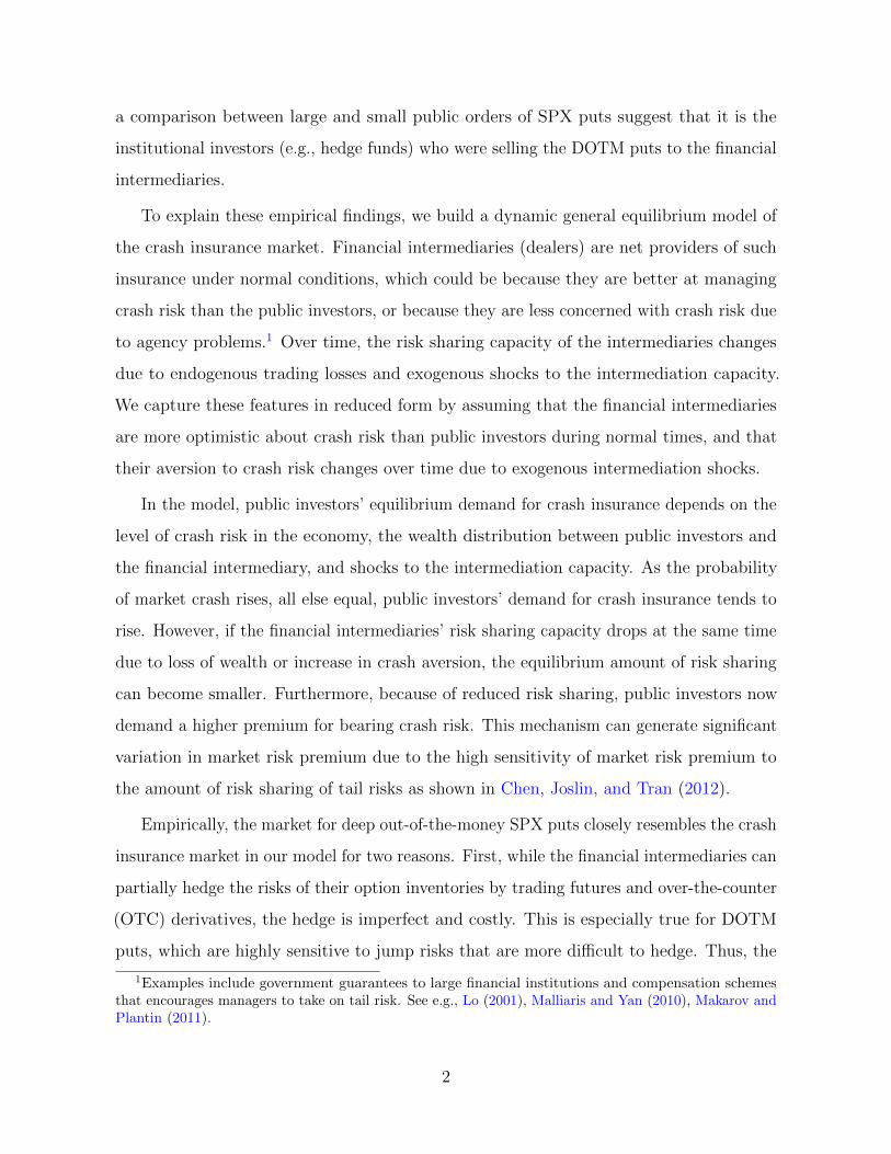
Figure 1: Time Series of net public purchase for DOTM SPX puts. The seriesplotted is the net amount of DOTM (with K/S ≤ 0.85) SPX puts public investors buy-to-open each month(PNBO). “Asian” (1997/12): period around the Asian financial crisis. “Russian” (1998/11): period aroundRussian default. “Iraq” (2003/04): start of the Iraq War. “Quant” (2007/08): the crisis of quant-strategyhedge funds. “Bear Sterns” (2008/03): acquisition of Bear Sterns by JPMorgan. “Lehman” (2008/09):Lehman bankruptcy. “TARP” (2008/10): establishment of TARP. “TALF1” (2008/11): creation of TALF.“BoA” (2009/01): Treasury, Fed, and FDIC assistance to Bank of America. “TALF2” (2009/02): increaseof TALF to $1 trillion. “Euro1” (2009/12): escalation of Greek debt crisis. “GB1” (2010/04): Greece seeksfinancial support from euro and IMF. “EFSF” (2010/05): establishment of EFSM and EFSF; 110 billionbailout package to Greece agreed. “GB2” (2010/09): a second Greek bailout installment. “Voluntary”(2011/06): Merkel agrees to voluntary Greece bondholder role. “Euro2” (2011/10): further escalation ofEuro debt crisis.

Figure 1 plots the time series of our main option volume measure, PNBO. Consistent

with the finding of GPP, the net public purchase for DOTM index puts is positive most of

the time prior to the recent financial crisis in 2008, suggesting that broker-dealers and

market-makers were net sellers of market crash insurance while public investors were net

buyers. A few exceptions include the period around the Asian financial crisis (1997/12),

the Russian default and the financial crisis in Latin America (1998/11-1999/01), the Iraq

War (2003/04), and twice in 2005 (2005/03 and 2005/11).2

2An economic event potentially associated with the negative PNBO in 2005 is the GM and Forddowngrade in 2005/05.

6

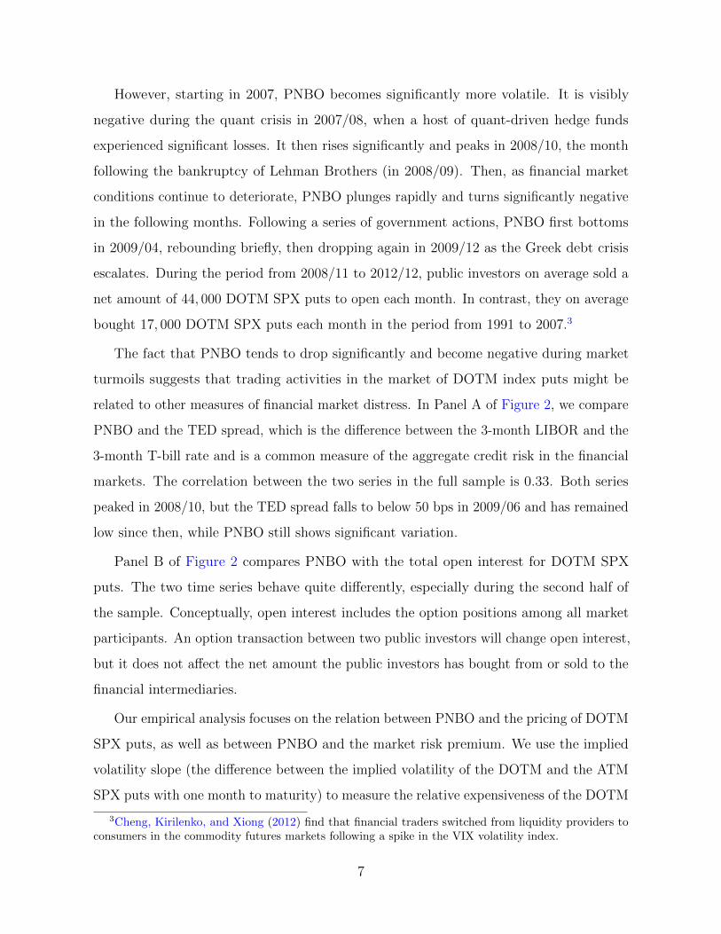
However, starting in 2007, PNBO becomes significantly more volatile. It is visibly

negative during the quant crisis in 2007/08, when a host of quant-driven hedge funds

experienced significant losses. It then rises significantly and peaks in 2008/10, the month

following the bankruptcy of Lehman Brothers (in 2008/09). Then, as financial market

conditions continue to deteriorate, PNBO plunges rapidly and turns significantly negative

in the following months. Following a series of government actions, PNBO first bottoms

in 2009/04, rebounding briefly, then dropping again in 2009/12 as the Greek debt crisis

escalates. During the period from 2008/11 to 2012/12, public investors on average sold a

net amount of 44, 000 DOTM SPX puts to open each month. In contrast, they on average

bought 17, 000 DOTM SPX puts each month in the period from 1991 to 2007.3

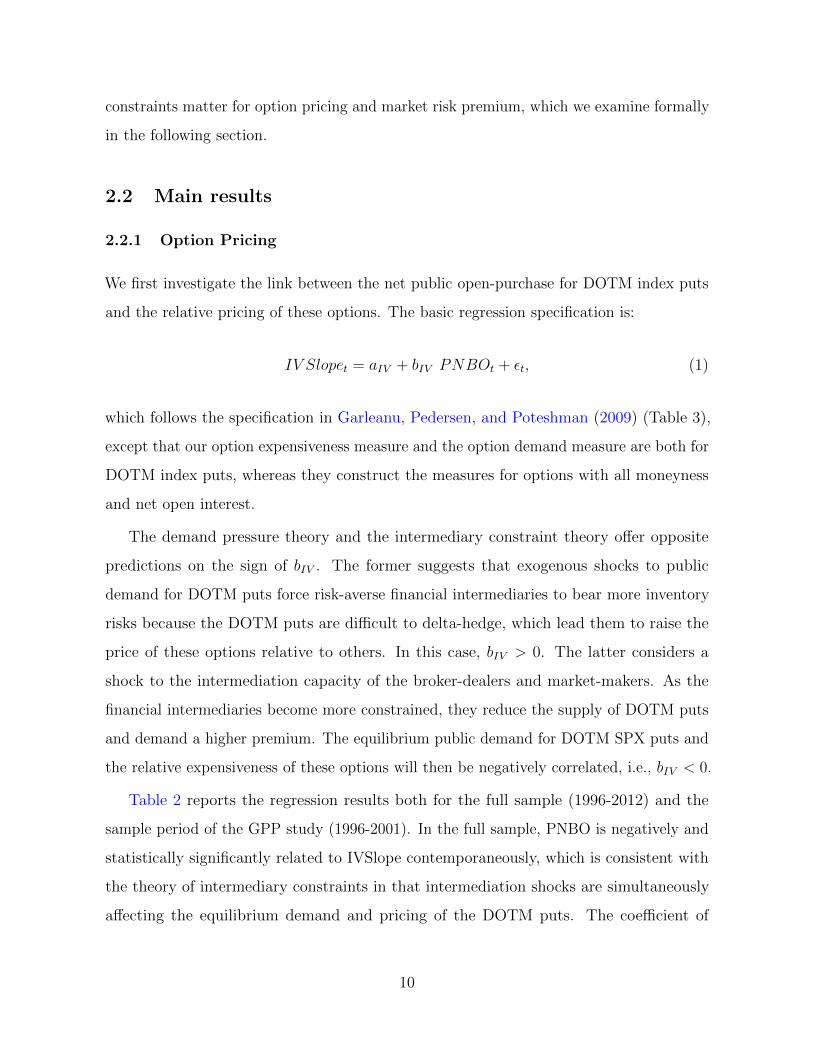
The fact that PNBO tends to drop significantly and become negative during market

turmoils suggests that trading activities in the market of DOTM index puts might be

related to other measures of financial market distress. In Panel A of Figure 2, we compare

PNBO and the TED spread, which is the difference between the 3-month LIBOR and the

3-month T-bill rate and is a common measure of the aggregate credit risk in the financial

markets. The correlation between the two series in the full sample is 0.33. Both series

peaked in 2008/10, but the TED spread falls to below 50 bps in 2009/06 and has remained

low since then, while PNBO still shows significant variation.

Panel B of Figure 2 compares PNBO with the total open interest for DOTM SPX

puts. The two time series behave quite differently, especially during the second half of

the sample. Conceptually, open interest includes the option positions among all market

participants. An option transaction between two public investors will change open interest,

but it does not affect the net amount the public investors has bought from or sold to the

financial intermediaries.

Our empirical analysis focuses on the relation between PNBO and the pricing of DOTM

SPX puts, as well as between PNBO and the market risk premium. We use the implied

volatility slope (the difference between the implied volatility of the DOTM and the ATM

SPX puts with one month to maturity) to measure the relative expensiveness of the DOTM

3Cheng, Kirilenko, and Xiong (2012) find that financial traders switched from liquidity providers toconsumers in the commodity futures markets following a spike in the VIX volatility index.

7

1990 1995 2000 2005 2010 2015−0.2

−0.1

0

0.1

0.2

PNBOTED

1990 1995 2000 2005 2010 20150

0.5

1

1.5

2

2.5A. PNBO vs. TED Spread

1990 1995 2000 2005 2010 2015−0.2

−0.1

0

0.1

0.2

PNBOOpen Interest

1990 1995 2000 2005 2010 20150

1

2

3

4

5B. PNBO vs. Open Interest

Figure 2: Comparing PNBO with TED spread and open interest. Open Interest ismeasured as the end-of-month total open interest for DOTM SPX puts (with K/S <= 0.85).PNBO and Open Interest are divided by 106. TED spread is in percentage. All the plottedseries are 6-month moving averages.

SPX puts. Market excess returns are computed using returns on the CRSP value-weighted

market index and the 1-month T-Bill returns. Besides PNBO, we also consider a range of

macro and financial variables that have been shown to be good predictors of the market

risk premium. These measures include the variance risk premium (VRP) by Bollerslev,

Tauchen, and Zhou (2009), the log price to earning ratio (p − e) and the log dividend

yield (d− p) of the market portfolio, the Baa-Aaa credit spread (DEF), the 10-year minus

3-month Treasury term spread (TERM), the tail risk measure (Tail) by Kelly (2012),

the consumption-wealth ratio measure (cay) by Lettau and Ludvigson (2001), and the

year-over-year change in broker-dealer leverage (∆lev) by Adrian, Moench, and Shin

(2010).

Table 1 reports the summary statistics of the variables used in our analysis. From

1991/01 to 2012/12, the net public open-purchase of the DOTM SPX puts (PNBO) is

close to 10, 000 contracts per month on average. In comparison, the average total open

interest for all DOTM SPX puts is around 1.4 million contracts during this period. For

the whole sample, even though the monthly net open-purchase by firm investors (FNBO)

is also positive on average (at 2686 contracts), the correlation between PNBO and FNBO

8

Table 1: Summary Statistics

mean median std AC(1) pp-test

PNBO (contracts) 9996 9665 51117 0.61 0.00PNB (contracts) 25799 12599.5 55634 0.37 0.00FNBO (contracts) 2686 -42.5 40567 0.37 0.00Open Interest (contracts) 1441710 899152 1442807 0.96 0.19IVSlope 16.20 15.33 3.76 0.81 0.42VRP 17.72 14.14 20.29 0.23 0.00p− e 3.14 3.08 0.31 0.98 0.63d− p -3.94 -4.00 0.30 0.98 0.89TED 0.44 0.35 0.37 0.85 0.00DEF 0.97 0.87 0.43 0.96 0.23TERM 1.84 1.97 1.21 0.98 0.32Tail 0.38 0.38 0.03 0.80 0.49cay 0.00 0.00 0.02 0.93 0.15∆lev 0.04 0.09 0.34 0.72 0.00

AC(1) is the first order autocorrelation; pp-test is the p-value for the Phillips-Perron test for unit

root. PNBO: net open-buying volume of DOTM index puts (K/S <= 0.85) by public investors.

PNB: public net buying volume of DOTM index puts. FNBO: net open-buying volume by firms.

Open Interest: end-of-month total open interest for all DOTM SPX puts. IVSlope: implied

volatility slope for SPX options. VRP: variance risk premium. p− e: log price to earning ratio.

d− p: log dividend yield. TED: TED spread. DEF: Baa-Aaa credit spread. TERM: 10y−3m

Treasury spread. Tail: tail risk measure from individual stocks. cay is the consumption-wealth

ratio measure. ∆lev is the year-over-year log growth rate in broker-dealer leverage. All data are

monthly except for cay and ∆lev, which are quarterly.

is −0.4, suggesting that firm investors, along with market makers, tend to be trading

against the public investors as a whole. Unlike the standard return predictors such as

price-earnings ratio, dividend yield, term spread, or consumption-wealth ratio, all of which

are highly persistent, the option volume measures have relatively modest autocorrelations

(e.g., 0.61 for PNBO and 0.37 for PNB).

The PNBO series is pro-cyclical, as indicated by its positive correlation with industrial

production growth (0.17) and negative correlation with unemployment rate (−0.48). In

addition, the correlation between PNBO and IVSlope is −0.46. Its correlation with changes

in broker-dealer leverage ∆lev is 0.50, and the correlation with the leading 3-month market

risk premium is −0.43. These results are consistent with the interpretation that dealer

9

constraints matter for option pricing and market risk premium, which we examine formally

in the following section.

2.2 Main results

2.2.1 Option Pricing

We first investigate the link between the net public open-purchase for DOTM index puts

and the relative pricing of these options. The basic regression specification is:

IV Slopet = aIV + bIV PNBOt + εt, (1)

which follows the specification in Garleanu, Pedersen, and Poteshman (2009) (Table 3),

except that our option expensiveness measure and the option demand measure are both for

DOTM index puts, whereas they construct the measures for options with all moneyness

and net open interest.

The demand pressure theory and the intermediary constraint theory offer opposite

predictions on the sign of bIV . The former suggests that exogenous shocks to public

demand for DOTM puts force risk-averse financial intermediaries to bear more inventory

risks because the DOTM puts are difficult to delta-hedge, which lead them to raise the

price of these options relative to others. In this case, bIV > 0. The latter considers a

shock to the intermediation capacity of the broker-dealers and market-makers. As the

financial intermediaries become more constrained, they reduce the supply of DOTM puts

and demand a higher premium. The equilibrium public demand for DOTM SPX puts and

the relative expensiveness of these options will then be negatively correlated, i.e., bIV < 0.

Table 2 reports the regression results both for the full sample (1996-2012) and the

sample period of the GPP study (1996-2001). In the full sample, PNBO is negatively and

statistically significantly related to IVSlope contemporaneously, which is consistent with

the theory of intermediary constraints in that intermediation shocks are simultaneously

affecting the equilibrium demand and pricing of the DOTM puts. The coefficient of

10

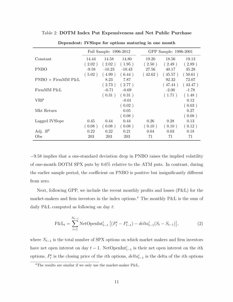
Table 2: DOTM Index Put Expensiveness and Net Public Purchase

Dependent: IVSlope for options maturing in one month

Full Sample: 1996-2012 GPP Sample: 1996-2001

Constant 14.44 14.58 14.80 19.20 18.56 19.13( 2.02 ) ( 2.02 ) ( 1.95 ) ( 2.50 ) ( 2.49 ) ( 2.89 )

PNBO -9.58 -10.23 -10.43 27.56 40.17 35.28( 5.02 ) ( 4.99 ) ( 6.44 ) ( 42.62 ) ( 45.57 ) ( 50.61 )

PNBO × FirmMM P&L 8.23 7.87 92.32 72.07( 2.73 ) ( 2.77 ) ( 47.44 ) ( 43.47 )

FirmMM P&L -0.71 -0.69 -2.00 -1.78( 0.31 ) ( 0.31 ) ( 1.71 ) ( 1.48 )

VRP -0.01 0.12( 0.02 ) ( 0.03 )

Mkt Return 0.05 0.27( 0.08 ) ( 0.08 )

Lagged IVSlope 0.45 0.44 0.44 0.26 0.28 0.13( 0.08 ) ( 0.08 ) ( 0.08 ) ( 0.10 ) ( 0.10 ) ( 0.12 )

Adj. R2 0.22 0.22 0.21 0.04 0.03 0.18Obs 203 203 203 71 71 71

−9.58 implies that a one-standard deviation drop in PNBO raises the implied volatility

of one-month DOTM SPX puts by 0.6% relative to the ATM puts. In contrast, during

the earlier sample period, the coefficient on PNBO is positive but insignificantly different

from zero.

Next, following GPP, we include the recent monthly profits and losses (P&L) for the

market-makers and firm investors in the index options.4 The monthly P&L is the sum of

daily P&L computed as following on day t:

P&Lt =

Nt−1∑i=1

NetOpenIntit−1

[(P i

t − P it−1)− deltait−1(St − St−1)

], (2)

where Nt−1 is the total number of SPX options on which market makers and firm investors

have net open interest on day t− 1. NetOpenIntit−1 is their net open interest on the ith

options, P it is the closing price of the ith options, deltait−1 is the delta of the ith options

4The results are similar if we only use the market-maker P&L.

11

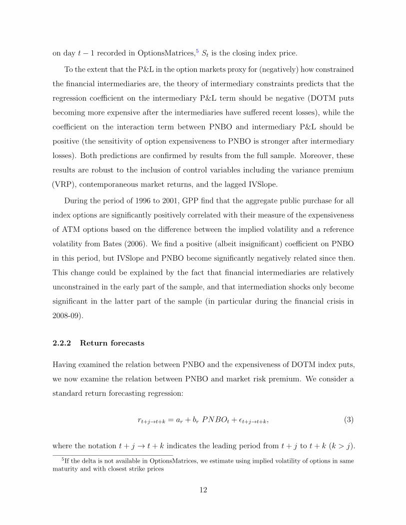
on day t− 1 recorded in OptionsMatrices,5 St is the closing index price.

To the extent that the P&L in the option markets proxy for (negatively) how constrained

the financial intermediaries are, the theory of intermediary constraints predicts that the

regression coefficient on the intermediary P&L term should be negative (DOTM puts

becoming more expensive after the intermediaries have suffered recent losses), while the

coefficient on the interaction term between PNBO and intermediary P&L should be

positive (the sensitivity of option expensiveness to PNBO is stronger after intermediary

losses). Both predictions are confirmed by results from the full sample. Moreover, these

results are robust to the inclusion of control variables including the variance premium

(VRP), contemporaneous market returns, and the lagged IVSlope.

During the period of 1996 to 2001, GPP find that the aggregate public purchase for all

index options are significantly positively correlated with their measure of the expensiveness

of ATM options based on the difference between the implied volatility and a reference

volatility from Bates (2006). We find a positive (albeit insignificant) coefficient on PNBO

in this period, but IVSlope and PNBO become significantly negatively related since then.

This change could be explained by the fact that financial intermediaries are relatively

unconstrained in the early part of the sample, and that intermediation shocks only become

significant in the latter part of the sample (in particular during the financial crisis in

2008-09).

2.2.2 Return forecasts

Having examined the relation between PNBO and the expensiveness of DOTM index puts,

we now examine the relation between PNBO and market risk premium. We consider a

standard return forecasting regression:

rt+j→t+k = ar + br PNBOt + εt+j→t+k, (3)

where the notation t+ j → t+ k indicates the leading period from t+ j to t+ k (k > j).

5If the delta is not available in OptionsMatrices, we estimate using implied volatility of options in samematurity and with closest strike prices

12

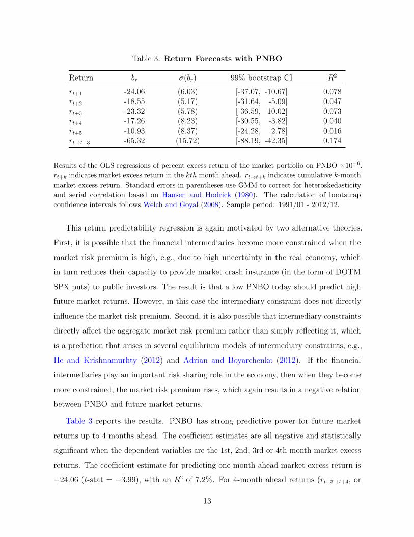
Table 3: Return Forecasts with PNBO

Return br σ(br) 99% bootstrap CI R2

rt+1 -24.06 (6.03) [-37.07, -10.67] 0.078rt+2 -18.55 (5.17) [-31.64, -5.09] 0.047rt+3 -23.32 (5.78) [-36.59, -10.02] 0.073rt+4 -17.26 (8.23) [-30.55, -3.82] 0.040rt+5 -10.93 (8.37) [-24.28, 2.78] 0.016rt→t+3 -65.32 (15.72) [-88.19, -42.35] 0.174

Results of the OLS regressions of percent excess return of the market portfolio on PNBO ×10−6.

rt+k indicates market excess return in the kth month ahead. rt→t+k indicates cumulative k-month

market excess return. Standard errors in parentheses use GMM to correct for heteroskedasticity

and serial correlation based on Hansen and Hodrick (1980). The calculation of bootstrap

confidence intervals follows Welch and Goyal (2008). Sample period: 1991/01 - 2012/12.

This return predictability regression is again motivated by two alternative theories.

First, it is possible that the financial intermediaries become more constrained when the

market risk premium is high, e.g., due to high uncertainty in the real economy, which

in turn reduces their capacity to provide market crash insurance (in the form of DOTM

SPX puts) to public investors. The result is that a low PNBO today should predict high

future market returns. However, in this case the intermediary constraint does not directly

influence the market risk premium. Second, it is also possible that intermediary constraints

directly affect the aggregate market risk premium rather than simply reflecting it, which

is a prediction that arises in several equilibrium models of intermediary constraints, e.g.,

He and Krishnamurhty (2012) and Adrian and Boyarchenko (2012). If the financial

intermediaries play an important risk sharing role in the economy, then when they become

more constrained, the market risk premium rises, which again results in a negative relation

between PNBO and future market returns.

Table 3 reports the results. PNBO has strong predictive power for future market

returns up to 4 months ahead. The coefficient estimates are all negative and statistically

significant when the dependent variables are the 1st, 2nd, 3rd or 4th month market excess

returns. The coefficient estimate for predicting one-month ahead market excess return is

−24.06 (t-stat = −3.99), with an R2 of 7.2%. For 4-month ahead returns (rt+3→t+4, or

13

simply rt+4), coefficient estimate is −17.26 (t-stat = −2.10), with an R2 of 3.6%. Beyond

4 months, the predictive coefficient br is no longer statistically significant. When we

aggregate the effect for the cumulative market excess returns in the next 3 months, the

coefficient estimate of −65.32 implies that a one-standard deviation decrease in PNBO

raises the future 3-month market excess return by 3.4%. The R2 is an impressive 17.4%.

Next, we compare the predictive power of PNBO with a series of financial and macro

variables that have been shown to predict market returns in the literature, including the

variance risk premium (VRP), the log price-earnings ratio (p− e), the log dividend yield

(d − p), the Baa-Aaa credit spread (DEF), the 10y-3m Treasury spread (TERM), the

consumption-wealth ratio (cay), and the year-over-year log growth rate in broker-dealer

leverage (∆lev). In addition, we also add the TED spread (TED) and the open interest

for DOTM SPX puts to the list of variables for comparison.

The results are reported in Table 4. For all alternative predictive variables, adding

PNBO significantly raises the adjusted R2 of the regression. Moreover, the coefficient on

PNBO remains negative and statistically significant, and the size of the coefficient is similar

across regressions. In contrast, only the variance risk premium, the log price-earnings ratio,

and the consumption-wealth ratio are statistically significantly after PNBO is included in

the regression.

The fact that the predictive power of PNBO remains statistically significant after

controlling for other standard predictive variables suggests that there is unique information

about market risk premium that is contained in option trading activities and not captured

by the standard macro and financial factors that drive risk premium. This potentially

allows us to disentangle the two alternative explanations of the negative relation between

PNBO and future market returns as discussed above. If the intermediary constraint as

proxied by PNBO merely reflects the aggregate risk premia rather than directly causing

the fluctuations in risk premia, then the inclusion of the actual risk factors should drive out

predictive power of PNBO. Of course, the evidence above does not prove that intermediary

constraints actually drive aggregate risk premia. It is always possible that PNBO is

correlated with some true risk factors that are not considered in our specifications.

14

Tab

le4:

Retu

rnFore

cast

sw

ith

PN

BO

and

Oth

er

Pre

dic

tors

mon

thly

regr

essi

onquar

terl

yre

gres

sion

VR

P0.

140.

090.

11(0

.02)

(0.0

4)(0

.05)

p−e

-0.6

9-3

.42

-2.4

0(2

.63)

(1.9

2)(1

.72)

d−p

4.92

2.76

6.01

(2.7

8)(2

.48)

(2.4

2)T

ED

-4.5

2-1

.76

-0.8

4(2

.94)

(2.1

4)(1

.52)

Op

enIn

t0.

43(0

.69)

DE

F-1

.07

(0.7

4)T

ER

M-1

.86

(2.1

5)cay

33.3

945

.32

(28.

29)

(27.

77)

∆lev

-8.1

5-3

.57

(2.9

4)(2

.79)

PN

BO

-52.

94-7

0.13

-62.

10-6

1.16

-49.

49-8

7.29

-72.

22(1

6.58

)(1

5.03

)(1

7.95

)(1

3.89

)(1

6.93

)(2

0.47

)(2

1.45

)A

djR

20.

120.

220.

000.

180.

030.

180.

040.

170.

000.

270.

000.

170.

090.

17O

bs

264

264

264

264

264

264

264

264

204

264

8787

8888

Res

ult

sof

the

OL

Sre

gres

sion

sof

per

cent

exce

ssre

turn

ofth

em

arke

tp

ortf

olio

onP

NB

Oan

dot

her

pre

dic

tors

.V

aria

nce

risk

pre

miu

m

(VR

P),

log

pri

ce-e

arnin

gsra

tio

(p−e)

,lo

gdiv

iden

dyie

ld(d−p),

TE

Dsp

read

(TE

D),

Baa

-Aaa

cred

itsp

read

(DE

F),

and

the

10-y

ear

and

3-m

onth

Tre

asury

term

spre

ad(T

ER

M)

are

use

din

the

mon

thly

regr

essi

ons,

whic

hfo

reca

sts

3-m

onth

ahea

dex

cess

mar

ket

retu

rns

r t→t+

3.

Con

sum

pti

on-w

ealt

hra

tio

(cay)

and

chan

ges

inB

roke

r-D

eale

rle

vera

ge(∆lev)

are

avai

lab

lequar

terl

y,w

hic

har

euse

dto

pre

dic

t

nex

t-quar

ter

exce

ssm

arke

tre

turn

ina

qu

arte

rly

regr

essi

on.

Sta

ndar

der

rors

inpar

enth

eses

use

GM

Mto

corr

ect

for

het

eros

kedas

tici

ty

and

seri

al

corr

elat

ion

bas

edon

Han

sen

an

dH

od

rick

(198

0).

Sam

ple

per

iod:

1991

/01

-20

12/1

2.

15

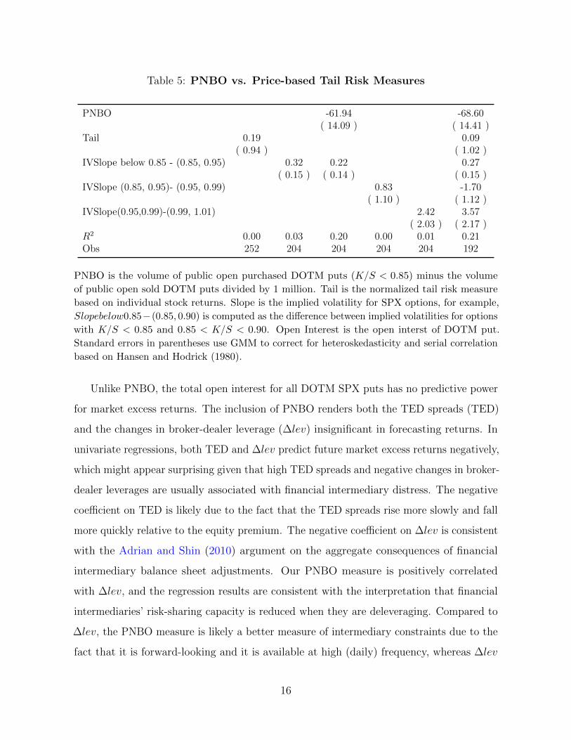
Table 5: PNBO vs. Price-based Tail Risk Measures

PNBO -61.94 -68.60( 14.09 ) ( 14.41 )

Tail 0.19 0.09( 0.94 ) ( 1.02 )

IVSlope below 0.85 - (0.85, 0.95) 0.32 0.22 0.27( 0.15 ) ( 0.14 ) ( 0.15 )

IVSlope (0.85, 0.95)- (0.95, 0.99) 0.83 -1.70( 1.10 ) ( 1.12 )

IVSlope(0.95,0.99)-(0.99, 1.01) 2.42 3.57( 2.03 ) ( 2.17 )

R2 0.00 0.03 0.20 0.00 0.01 0.21Obs 252 204 204 204 204 192

PNBO is the volume of public open purchased DOTM puts (K/S < 0.85) minus the volume

of public open sold DOTM puts divided by 1 million. Tail is the normalized tail risk measure

based on individual stock returns. Slope is the implied volatility for SPX options, for example,

Slopebelow0.85−(0.85, 0.90) is computed as the difference between implied volatilities for options

with K/S < 0.85 and 0.85 < K/S < 0.90. Open Interest is the open interst of DOTM put.

Standard errors in parentheses use GMM to correct for heteroskedasticity and serial correlation

based on Hansen and Hodrick (1980).

Unlike PNBO, the total open interest for all DOTM SPX puts has no predictive power

for market excess returns. The inclusion of PNBO renders both the TED spreads (TED)

and the changes in broker-dealer leverage (∆lev) insignificant in forecasting returns. In

univariate regressions, both TED and ∆lev predict future market excess returns negatively,

which might appear surprising given that high TED spreads and negative changes in broker-

dealer leverages are usually associated with financial intermediary distress. The negative

coefficient on TED is likely due to the fact that the TED spreads rise more slowly and fall

more quickly relative to the equity premium. The negative coefficient on ∆lev is consistent

with the Adrian and Shin (2010) argument on the aggregate consequences of financial

intermediary balance sheet adjustments. Our PNBO measure is positively correlated

with ∆lev, and the regression results are consistent with the interpretation that financial

intermediaries’ risk-sharing capacity is reduced when they are deleveraging. Compared to

∆lev, the PNBO measure is likely a better measure of intermediary constraints due to the

fact that it is forward-looking and it is available at high (daily) frequency, whereas ∆lev

16

1990 1995 2000 2005 2010 2015−40

−30

−20

−10

0

10

20

30Predicted vs. Realized 3-Month Market Excess Returns

predictedrealized

Figure 3: Return predictability in the time series. We compare the predicted vs.realized 3-month excess returns on the market portfolio.

is available quarterly with added reporting delay.

Besides the standard predictive variables in Table 4, we also compare PNBO with

several price-based tail risk measures, including the tail risk measure by Kelly (2012)

(based on equity return information), and the implied volatility slope measures based on

different moneyness. Table 5 shows that the IVslope measure from one month DOTM

puts (for K/S ≤ 0.85 vs. K/S ∈ (0.85, 0.95)) are statistically significantly related future

3 month returns (t-stat=2.13) in the univariate regression, and becomes insignificant

(t-stat=1.57) after controlling for PNBO. However, IVSlope measured from OTM puts has

no power in predicting returns. Finally, in a joint regression, none of the price-based tail

risk measures can account for the predictive power of PNBO.

The time variation in the predictive power of PNBO is illustrated in Figure 3, which

compares the realized 3-month excess returns on the market portfolio against those

predicted by option volume. The improvement in the model performance is quite visible

in the period starting in 2005. In particular, the PNBO-predicted market excess returns

closely replicated the major swings in the realized returns in the period post Lehman

17

2000 2002 2004 2006 2008 2010−0.05

0

0.05

0.1

0.15

0.2

0.25

0.3

0.35

0.4R

2A. Out-of-Sample R2

1995 2000 2005 2010 20150

0.1

0.2

0.3

0.4

0.5

R2

B. 5-Year Moving-Window R2

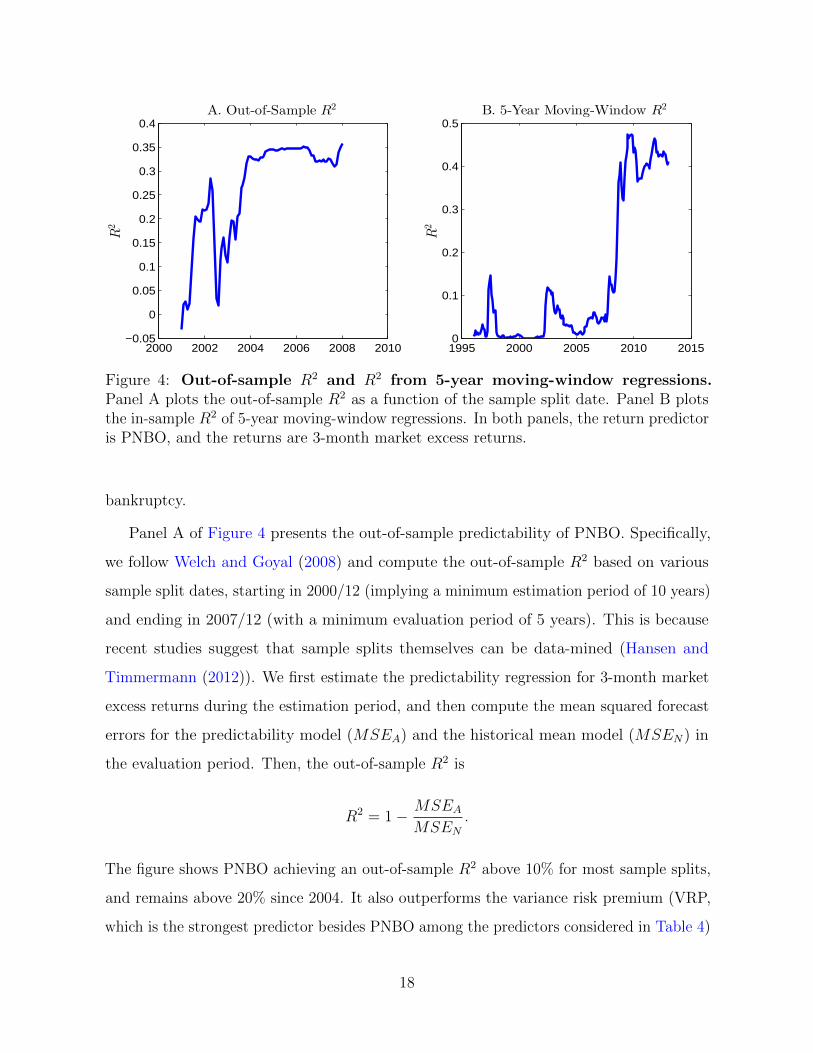
Figure 4: Out-of-sample R2 and R2 from 5-year moving-window regressions.Panel A plots the out-of-sample R2 as a function of the sample split date. Panel B plotsthe in-sample R2 of 5-year moving-window regressions. In both panels, the return predictoris PNBO, and the returns are 3-month market excess returns.

bankruptcy.

Panel A of Figure 4 presents the out-of-sample predictability of PNBO. Specifically,

we follow Welch and Goyal (2008) and compute the out-of-sample R2 based on various

sample split dates, starting in 2000/12 (implying a minimum estimation period of 10 years)

and ending in 2007/12 (with a minimum evaluation period of 5 years). This is because

recent studies suggest that sample splits themselves can be data-mined (Hansen and

Timmermann (2012)). We first estimate the predictability regression for 3-month market

excess returns during the estimation period, and then compute the mean squared forecast

errors for the predictability model (MSEA) and the historical mean model (MSEN) in

the evaluation period. Then, the out-of-sample R2 is

R2 = 1− MSEAMSEN

.

The figure shows PNBO achieving an out-of-sample R2 above 10% for most sample splits,

and remains above 20% since 2004. It also outperforms the variance risk premium (VRP,

which is the strongest predictor besides PNBO among the predictors considered in Table 4)

18

Table 6: Return Forecasts with Various SPX Option Volume Measures

Return br σ(br) R2 br σ(br) R2 br σ(br) R2

PNBO full-sample PNBO pre-crisis PNBO post-crisis

rt+1 -24.06 (6.03) 0.08 -18.49 (9.17) 0.01 -15.82 (11.55) 0.04rt→t+3 -65.32 (15.72) 0.17 -54.02 (19.62) 0.03 -40.48 (20.76) 0.13

PNBO/Total V ol PNB FNBO

rt+1 -114.77 (39.04) 0.03 -22.72 (4.45) 0.08 13.74 (7.90) 0.01rt→t+3 -291.16 (106.02) 0.07 -49.13 (16.63) 0.11 40.71 (18.35) 0.04

Results of the OLS regressions of percent excess return of the market portfolio on PNBO in

different subsamples and on alternative option volume measures. rt+1 indicates market excess

return one month ahead. PNBO/Total V ol is PNBO normalized by the average total SPX

volume in the previous 12 months. PNB is the public net buying volume (including both open and

close orders). FNBO is the firm net buying-to-open volume. rt→t+k indicates cumulative k-month

market excess return. Standard errors in parentheses use GMM to correct for heteroskedasticity

and serial correlation based on Hansen and Hodrick (1980). Full sample period: 1991/01 -

2012/12. Pre-crisis: 1991/01 - 2007/11. Post-crisis: 2009/06 - 2012/12.

in predicting 3-month returns across all sample splits.

Panel B of Figure 4 plots the in-sample R2 from the predictive regressions of PNBO

using 5-year moving windows. The R2 varies significantly over time. Consistent with

Figure 3, R2 is generally low in the early parts of the sample, being less than 5% most of

the time prior to 2006. It rises to 15% in the period around the Asian financial crisis and

Russian default in 1997-98, then to about 10% around 2002. During the crisis period, the

R2 rises to close to 50%. Since such high R2 would translate into striking Sharpe ratios

for investment strategies that try to exploit such predictability, the fact that they persist

during the financial crisis can be interpreted as evidence of the financial constraints that

prevent arbitrageurs from taking advantages of such investment opportunities.

In Table 6, we report the results of several robustness tests on PNBO. In the first

row, we compare the regression results of PNBO in the full sample (1991/01-2012/12)

against the results from two sub-samples: pre-crisis (1991/01-2007/11) and post-crisis

19

(2009/06-2012/12). The predictive power of PNBO remains statistically significant in both

sub-samples but is weaker than the full sample, both in terms of lower R2 and weaker

statistical significance of br. These results show that the relation between option trading

activities and market risk premium is stronger during the financial crisis, but it is not a

phenomenon that occurs exclusively in the financial crisis. The weaker predictive power for

PNBO in the earlier parts of the sample period could be due to the fact that intermediary

constraint is not as significant and variable in the first half of the sample as in the second

half (especially the crisis period). Another possible reason is that the options market was

under-developed in the early periods of the sample and did not play as important a role in

facilitating risk sharing as it does today.

Indeed, Figure 1 shows that PNBO is significantly more volatile in the second half

of the sample, which is in part due to the dramatic growth of the trading volume in

the options market during our sample period. To account for this effect, we normalize

PNBO by the past 12-month average SPX total trading volume. As Table 6 shows, this

normalized PNBO also predicts future one-month and 3-month cumulative market excess

returns significantly.

PNBO reflects public investors’ newly established positions. The net supply of DOTM

puts from the market makers in a given period not only includes the newly established

positions, but also the changes in existing positions. To measure this supply, we compute

PNB as the sum of net open- and close-buying volumes for public investors. Comparing

PNB with PNBO, the coefficient br and R2 essentially remain the same for the one-month

ahead return forecast. In the cumulative 3-month return forecast, the R2 falls and br drops

in absolute value.

We also examine the predictability of the net-open-buying volume from firm investors

(FNBO). We can see that the firm investors net demand predict returns positively. This

result is consistent with the interpretation that both broker-dealers and market makers

have positions opposite to the public investors.

Next, we examine the robustness of PNBO predictive power based on how deep out-of-

the-money puts are classified. Our baseline definition of DOTM puts uses a very simple

20

0.75 0.8 0.85 0.9 0.95 1 1.05−120

−100

−80

−60

−40

−20

0A. Puts

K/S ≤ k

bret95% bootstrap C.I.

0.75 0.8 0.85 0.9 0.95 1 1.05−200

−100

0

100

200

300B. Calls

K/S ≤ k

−2 −1.5 −1 −0.5 0 0.5−40

−30

−20

−10

0C. Puts

K/S ≤ 1 + kσ−2 −1.5 −1 −0.5 0 0.5

−150

−100

−50

0

50

100

150D. Calls

K/S ≤ 1 + kσ

Figure 5: Alternative definitions of moneyness. In Panels A and B, PNBO ismeasured based on put options with K/S less than a constant cutoff k. In Panels C and D,PNBO is measured on put options with K/S less than 1 + kσ, where k is a constant, andσ represents a maturity-adjusted return volatility, which is the daily S&P return volatilityin the previous 30 trading days multiplied by the square root of the days to maturity forthe option.

cutoff rule K/S ≤ 0.85. A natural question is how the results change as we vary this cutoff.

The answer is shown in Panel A of Figure 5. The coefficient br in the return forecast

regression is consistently negative for a wide range of moneyness cutoffs. On the one

hand, br becomes more negative as the cutoff k becomes lower, i.e., when we measure the

net public open-purchase for deeper out-of-the-money puts. On the other hand, because

far out-of-money options are more thinly traded, the PNBO series becomes more noisy,

which widens the confidence interval on br. In contrast, for almost all moneyness cutoffs,

a PNBO measure based on SPX calls does not predict returns.

An objection to the definition of DOTM puts above is that a constant strike-to-price

21

cutoff implies different actual moneyness (e.g., as measured by option delta) for options

with different maturities. A 15% drop in price might seem very extreme in one day, but it

becomes much more likely in one year. For this reason, we examine a maturity-adjusted

moneyness definition. Specifically, we classify a put option as DOTM when

K/S ≤ 1 + kσt√T ,

where k is a constant, σt is the daily S&P return volatility in the previous 30 trading

days, and T is the days to maturity for the option. Panel C of Figure 5 shows that this

alternative classification of DOTM puts produces similar results as the simple cutoff rule.

Once again, Panel D shows that the PNBO series based on call options does not predict

returns.

2.3 Determinants of the demand for DOTM puts

In this section, we investigate the determinants of demand for crash insurance. In our

model, the dealers are less willing to provide crash insurance when they become more

averse to jump risk. Such rise in risk aversion is a proxy for the fact the dealers are

becoming more constrained. In this section, we present empirical evidence that the net

public purchase for DOTM SPX puts is indeed connected to dealer constraints.

Table 7 shows that PNBO is significantly positively related to changes in broker-dealer

leverage. Consistent with the results in Table 2, PNBO is also significantly negatively

related to the slope of implied volatility of SPX options. In addition, from its positive

relation with industrial productivity and negative relation with unemployment rate, we

can see that the public purchase of DOTM SPX puts is high when the economy in a good

state.

We further examine the relationship between the public demand for DOTM and changes

in leverage by exploring the Granger causality. We do this by forming a bivariate VAR and

testing for the significance of either public demand for DOTM in predicating future changes

in leverage or vice versa. In both cases, we find evidence that Granger causality runs both

22

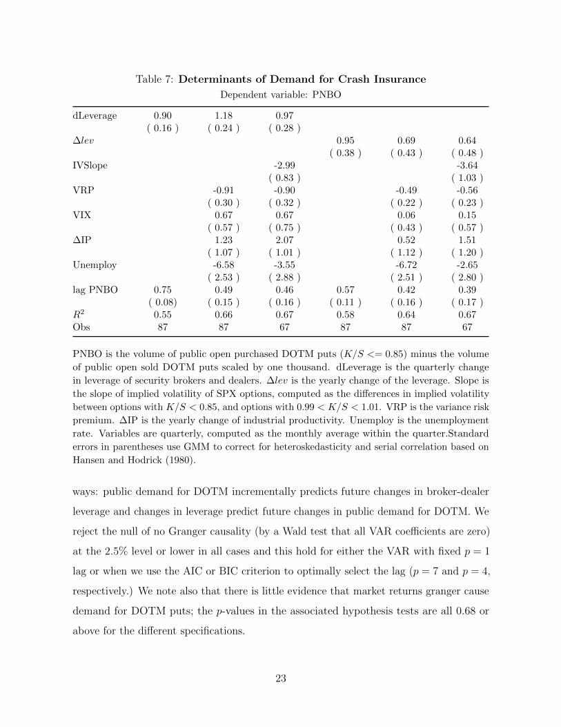
Table 7: Determinants of Demand for Crash Insurance

Dependent variable: PNBO

dLeverage 0.90 1.18 0.97( 0.16 ) ( 0.24 ) ( 0.28 )

∆lev 0.95 0.69 0.64( 0.38 ) ( 0.43 ) ( 0.48 )

IVSlope -2.99 -3.64( 0.83 ) ( 1.03 )

VRP -0.91 -0.90 -0.49 -0.56( 0.30 ) ( 0.32 ) ( 0.22 ) ( 0.23 )

VIX 0.67 0.67 0.06 0.15( 0.57 ) ( 0.75 ) ( 0.43 ) ( 0.57 )

∆IP 1.23 2.07 0.52 1.51( 1.07 ) ( 1.01 ) ( 1.12 ) ( 1.20 )

Unemploy -6.58 -3.55 -6.72 -2.65( 2.53 ) ( 2.88 ) ( 2.51 ) ( 2.80 )

lag PNBO 0.75 0.49 0.46 0.57 0.42 0.39( 0.08) ( 0.15 ) ( 0.16 ) ( 0.11 ) ( 0.16 ) ( 0.17 )

R2 0.55 0.66 0.67 0.58 0.64 0.67Obs 87 87 67 87 87 67

PNBO is the volume of public open purchased DOTM puts (K/S <= 0.85) minus the volume

of public open sold DOTM puts scaled by one thousand. dLeverage is the quarterly change

in leverage of security brokers and dealers. ∆lev is the yearly change of the leverage. Slope is

the slope of implied volatility of SPX options, computed as the differences in implied volatility

between options with K/S < 0.85, and options with 0.99 < K/S < 1.01. VRP is the variance risk

premium. ∆IP is the yearly change of industrial productivity. Unemploy is the unemployment

rate. Variables are quarterly, computed as the monthly average within the quarter.Standard

errors in parentheses use GMM to correct for heteroskedasticity and serial correlation based on

Hansen and Hodrick (1980).

ways: public demand for DOTM incrementally predicts future changes in broker-dealer

leverage and changes in leverage predict future changes in public demand for DOTM. We

reject the null of no Granger causality (by a Wald test that all VAR coefficients are zero)

at the 2.5% level or lower in all cases and this hold for either the VAR with fixed p = 1

lag or when we use the AIC or BIC criterion to optimally select the lag (p = 7 and p = 4,

respectively.) We note also that there is little evidence that market returns granger cause

demand for DOTM puts; the p-values in the associated hypothesis tests are all 0.68 or

above for the different specifications.

23

2.4 Who sold the DOTM puts in the crisis?

As Figure 1 shows, the amount of DOTM SPX puts that public investors sold to the

broker-dealers and market makers in the period following the Lehman bankruptcy is quite

large. It will be useful to find out who among the public investors sold the crash insurance

to the constrained financial intermediaries during the crisis. However, the SPX volume

data do not separate trades by retail investors from those by institutional investors. We

use two strategies to answer this question. First, we compare the trading activities of

the public investors in SPX options with those in SPY options. Second, we compare the

trading activities of large against small orders in SPX options.

While SPX and SPY options have essentially identical underlying asset, it is well

known among practitioners that SPX option volume has a significantly higher percentage

of institutional investors. Compared to retail investors, institutional investors prefer SPX

options more due to a larger contract size (10 times as large as SPY), cash settlement,

more favorable tax treatment, as well as being more capable of trading in between the

relatively wide bid-ask spreads of SPX options.

Thus, as in SPX options, we construct PNBOSPY for SPY options. Our SPY options

volume data are from the CBOE and ISE, and cover the period from 2005/01 to 2012/12.

Unlike the SPX options which trade exclusively on the CBOE, the SPY options are

cross-listed at several option exchanges. Our SPY PNBO variable aggregates the volume

data from the CBOE and ISE, which account for about half of the total trading volume

for SPY options.

During the period of 2005/01 to 2012/01, PNBOSPY is positive in most months,

suggesting that the public investors in the SPY market have been consistently buying

DOTM puts. From 2008/09 to 2010/12, PNBOSPX (or PNBO) is negative in 22 out of 28

months, whereas PNBOSPY is negative in just 7 of the months. The correlation between

PNBOSPY and PNBOSPX during this period is −0.27.

We also compare the ability of PNBOSPY and PNBOSPX in predicting market excess

returns. As Table 8 shows, PNBOSPY has no significant predictive power for future market

24

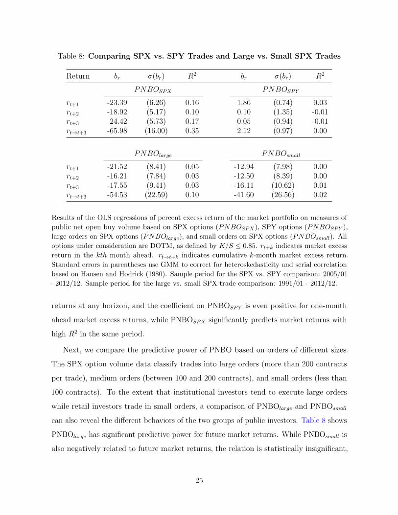
Table 8: Comparing SPX vs. SPY Trades and Large vs. Small SPX Trades

Return br σ(br) R2 br σ(br) R2

PNBOSPX PNBOSPY

rt+1 -23.39 (6.26) 0.16 1.86 (0.74) 0.03rt+2 -18.92 (5.17) 0.10 0.10 (1.35) -0.01rt+3 -24.42 (5.73) 0.17 0.05 (0.94) -0.01rt→t+3 -65.98 (16.00) 0.35 2.12 (0.97) 0.00

PNBOlarge PNBOsmall

rt+1 -21.52 (8.41) 0.05 -12.94 (7.98) 0.00rt+2 -16.21 (7.84) 0.03 -12.50 (8.39) 0.00rt+3 -17.55 (9.41) 0.03 -16.11 (10.62) 0.01rt→t+3 -54.53 (22.59) 0.10 -41.60 (26.56) 0.02

Results of the OLS regressions of percent excess return of the market portfolio on measures of

public net open buy volume based on SPX options (PNBOSPX), SPY options (PNBOSPY ),

large orders on SPX options (PNBOlarge), and small orders on SPX options (PNBOsmall). All

options under consideration are DOTM, as defined by K/S ≤ 0.85. rt+k indicates market excess

return in the kth month ahead. rt→t+k indicates cumulative k-month market excess return.

Standard errors in parentheses use GMM to correct for heteroskedasticity and serial correlation

based on Hansen and Hodrick (1980). Sample period for the SPX vs. SPY comparison: 2005/01

- 2012/12. Sample period for the large vs. small SPX trade comparison: 1991/01 - 2012/12.

returns at any horizon, and the coefficient on PNBOSPY is even positive for one-month

ahead market excess returns, while PNBOSPX significantly predicts market returns with

high R2 in the same period.

Next, we compare the predictive power of PNBO based on orders of different sizes.

The SPX option volume data classify trades into large orders (more than 200 contracts

per trade), medium orders (between 100 and 200 contracts), and small orders (less than

100 contracts). To the extent that institutional investors tend to execute large orders

while retail investors trade in small orders, a comparison of PNBOlarge and PNBOsmall

can also reveal the different behaviors of the two groups of public investors. Table 8 shows

PNBOlarge has significant predictive power for future market returns. While PNBOsmall is

also negatively related to future market returns, the relation is statistically insignificant,

25

and the R2 is much smaller. These comparisons suggest that it is the institutional investors

who sold the DOTM put options to the financial intermediaries during the crisis period.

3 A Dynamic Model

In Section 2, we document a number of features of the market for crash insurance. In

particular, there is time-varying equilibrium demand for crash insurance from public

investors. The equilibrium demand is inversely related to the relative price of the out-of-

the-money put protection—times in which the equilibrium demand is low are generally

times when the protection is very expensive. The demand for crash insurance was also

informative about future stock market returns over and above the information in option

prices and macro-variables. We now examine an equilibrium model consistent with these

empirical facts.

As our model elaborates, the main mechanism we have in mind is a model whereby

a public sector and intermediary face time-varying risk of a disaster. In general, the

intermediary is more willing to bear the downside risk of the disaster. However, as the

amount of risk rises, the intermediary becomes less willing (or less able) to share the risk

of a crash. These ingredients allow us to capture our key empirical results.

3.1 A Simple Model with Intermediary Constraints

We first consider a simple model that illustrates the main mechanism for the negative

relationship between public purchase of out-of-the-money options and subsequent market

returns. The key feature of our model will be that as the amount of risk rises, the public

demand curve will (necessarily) shift up, but the equilibrium demand will go down. This

will follow because the dealer’s supply curve will shift up more and the market clearly price

will imply the lower equilibrium quantity. In our simple model, this will follow because

the dealer faces a tighter capital constraints. This suggests that the tightness of dealer

constraints can be understood in reduced form as time-variation in effective risk aversion,

an observation made by Adrian and Shin (2010), He and Krishnamurhty (2012), Cochrane

26

0 0.02 0.04 0.06 0.08 0.1 0.12 0.14 0.16 0.18 0.20

0.2

0.4

0.6

0.8

1

1.2

1.4

1.6

1.8

2

price

quantit

y

Supply λ=1%

Demand λ=1%

Supply λ=3%

Demand λ=3%

Supply λ=3%, γ=7.6

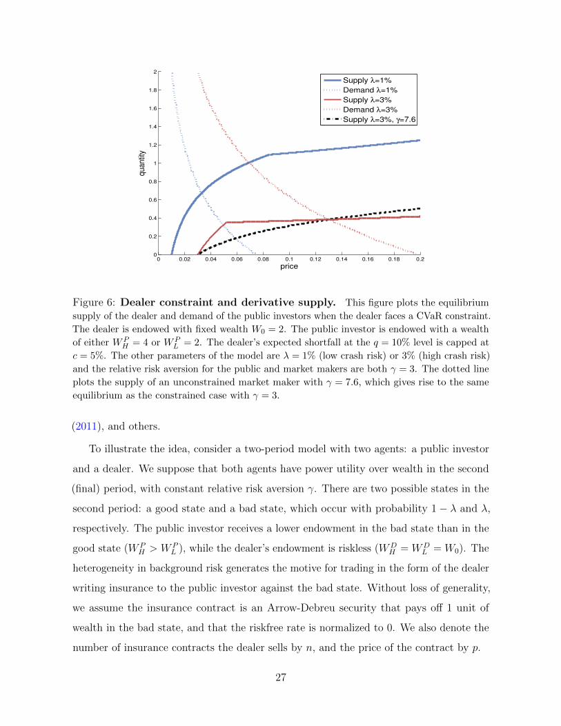
Figure 6: Dealer constraint and derivative supply. This figure plots the equilibrium

supply of the dealer and demand of the public investors when the dealer faces a CVaR constraint.

The dealer is endowed with fixed wealth W0 = 2. The public investor is endowed with a wealth

of either WPH = 4 or WP

L = 2. The dealer’s expected shortfall at the q = 10% level is capped at

c = 5%. The other parameters of the model are λ = 1% (low crash risk) or 3% (high crash risk)

and the relative risk aversion for the public and market makers are both γ = 3. The dotted line

plots the supply of an unconstrained market maker with γ = 7.6, which gives rise to the same

equilibrium as the constrained case with γ = 3.

(2011), and others.

To illustrate the idea, consider a two-period model with two agents: a public investor

and a dealer. We suppose that both agents have power utility over wealth in the second

(final) period, with constant relative risk aversion γ. There are two possible states in the

second period: a good state and a bad state, which occur with probability 1− λ and λ,

respectively. The public investor receives a lower endowment in the bad state than in the

good state (W PH > W P

L ), while the dealer’s endowment is riskless (WDH = WD

L = W0). The

heterogeneity in background risk generates the motive for trading in the form of the dealer

writing insurance to the public investor against the bad state. Without loss of generality,

we assume the insurance contract is an Arrow-Debreu security that pays off 1 unit of

wealth in the bad state, and that the riskfree rate is normalized to 0. We also denote the

number of insurance contracts the dealer sells by n, and the price of the contract by p.

27

Next, we assume that the dealer faces an exogenous constraint on his total risk exposure.

Specifically, the constraint is that the conditional Value-at-Risk (CVaR) at level q cannot

exceed a fraction c of his wealth. The CVaR, which is also referred to as the expected

shortfall, is defined as the average value-at-risk (VaR) with confidence level from 0 to q:

ESq = E[loss|being in worst q% tail] =1

q

∫ q

0

V aRαdα. (4)

The resulting equilibrium is plotted in Figure 6, where we consider the cases of a low

and high probability of disaster. We see that as the amount of risk rises, the demand

curve for the public rises. However, at the same time the supply curve falls and the CVaR

constraint begins to bind. The result is that as risk rises, the equilibrium quantity falls.

Moreover, as indicated by the dashed black line, the same equilibrium quantity would be

obtained if instead of the constraint binding more with higher levels of risk, the dealer

was instead more risk averse as the amount of risk went up.

This simple comparative static exercise shows that the relationship between the about

of risk and the amount of trade depends crucially on how the risk-sharing capacity of the

dealer changes with the level of crash risk in the economy. In reality, the dealers are large

financial institutions, and many factors could changes their risk-sharing capacity, including

losses in wealth from other investments, regulatory changes on capital requirement, and

beliefs about government guarantees. Another observation from this example is that we

can arrive at the same equilibrium if instead of imposing the CVaR constraint, we assume

the dealer’s risk aversion rises as the crash risk increases.

It is worth noting that this mechanism differs from other studies that focus on market

makers or arbitrageurs to share risk with public investors with exogenous stochastic demand.

For example, in Garleanu, Pedersen, and Poteshman (2009), demand is specified as an

exogenous process. Vayanos and Vila (2009) and Greenwood and Vayanos (2012) also focus

on public investors who have exogenous demand curves. In these papers, public investors

are models as having flat demand curve (or alternatively as having exogenously specified

equilibrium demand). Such approaches cannot immediately reconcile our empirical finding

28

without introducing the possibility or correlation between the risk bearing capacity of the

market makers with the public demand.

3.2 A Full Dynamic Model

We now present a dynamic model for the market of crash insurance. Our model builds

on Chen, Joslin, and Tran (2012) which is based on disagreement about a time-varying

disaster probability. We extend their model by incorporating time-variation in the dealer’s

aversion to crash risk. Similar alternative models could be based purely on time-varying

risk aversion or dealer constraints.

We consider an aggregate endowment in the economy which follows a jump diffusion

process where the endowment is subject to both a diffusive risk and a jump risk. In

particular, sudden severe drops in the aggregate endowment are a source of disaster risk

in this economy. There are two types of agents in the economy: small public investors

and competitive dealers. We assume there exists a representative public investor, who is

denoted by agent P , and a representative dealer, denoted by agent D. To induce the two

types of agents to trade, we assume that they have different beliefs about the probability

of disasters. As discussed earlier, such differences in beliefs capture in reduced form the

advantages that dealers have in bearing disaster risk, whether it is due to differences in

technology, agency problems, or behavioral biases.

Specifically, we assume that both agents believe that the log aggregate endowment

ct = logCt follows the process

dct = gdt+ σcdWct − d dNt (5)

where g and σc are the expected growth rate and volatility of consumption without jumps,

W ct is a standard Brownian motion under both agents’ beliefs, d is the constant size

of consumption drop in a diaster6. Nt is a counting process whose jumps arrive with

6As in Chen, Joslin, and Tran (2012), one could generalize the model by allowing disaster size to havea time-invariant distribution.

29

stochastic intensity λt under the public investors’ beliefs,

dλt = κ(λ− λt)dt+ σλ√λtdW

λt , (6)

where λ is the long-run average jump intensity under P ’s beliefs, and W λt is a standard

Brownian motion independent of W ct . In general, the dealers are more willing to bear

the disaster risk because (they act as if) they are more optimistic about disaster risk.

We assume that they believe that the disaster intensity is given by ρλt with ρ < 1. We

summarize the public investors’ beliefs with the probability measure PP , and the dealers’

beliefs with the probability measure PD.

Public investors have standard constant relative risk aversion (CRRA) utility:

UP = EP0

[∫ ∞0

e−δtC1−γP,t

1− γdt

], (7)

where we focus on the cases where γ > 1. The superscript P reflects that the expectations

are taken under the public investors’ beliefs.

The utility function of the dealers are different. We assume that the dealers face an

intermediation constraint that we model in a reduced form directly in terms of their utility.

Specifically, we suppose that

UD = ED0

[∫ ∞0

e−δtC1−γD,t

1− γe−

∑Ntn=1(ατ(n)−α)dt

], (8)

where αt is a stochastic variable representing the ability of the dealer to intermediate

disaster risk. Limited ability to intermediate risk is modeled as increased risk aversion

against market crashes. The specification generalizes the state-dependent preferences

proposed by Bates (2008) in that it allows the dealers’ risk aversion against crashes to rise

with the probability of disasters.

Specifically, τ(n) is the time of the nth disaster since t = 0, τ(n) ≡ inf{s : Ns = n}

Thus, this crash-aversion term remains constant in between disasters. Suppose the dealer’s

log consumption drops by dD,τ(n) at the time of the nth disaster. Then, at the same time,

30

the marginal utility of the dealer jumps up by

eγdD,τ(n)−(ατ(n)−α) = e

(γ−

ατ(n)−α)

dD,τ(n)

)dD,τ(n)

,

which implies that the dealer’s effective relative risk aversion against the disaster is

γD,τ(n) = γ −ατ(n) − αdD,τ(n)

. (9)

Thus, when αt > α, the dealers will have lower aversion to disaster risk than public

investors. As αt falls, the dealer’s effective risk aversion rises.

The intermediation capacity of the dealers may be related to the disaster intensity.

We model the intermediation as being driven jointly by the disaster intensity, λt, and an

independent factor, xt, so that αt = −aλt + bxt. Thus when a > 0, the intermediation

capacity goes down as the intensity rises and the dealer becomes more averse to disaster

risk.

Any jointly affine process for (ct, λt, xt) would be suitable for a tractable specification.

For example, we could suppose that xt follows an independent CIR process:

dxt = κx(x− xt)dt+ σx√xtdW

xt . (10)

In our calibrations, we will choose the simple specification with b = 0 so that the

intermediation capacity is perfectly correlated with the disaster intensity.

The main motivation for dealers’ time-varying aversion to crash risk is the time-varying

constraint faced by financial intermediaries. Rising crash risk in the economy raises

the intermediaries’ capital/collateral requirements and tightens their constraints on tail

risk exposures (e.g., Value-at-Risk constraints), which make them more reluctant to

provide insurance against disaster risk. For example, see Adrian and Shin (2010), He and

Krishnamurhty (2012). In this sense, the shocks to the disaster intensity in the model

also serve the purpose of generating time variation in the intermediation capacity of the

dealers. We can further generalize the specification by making the dealers’ aversion to

31

crash risk driven by adding independent variations in the intermediation shocks.

We also assume that markets are complete and agents are endowed with some fixed

share of aggregate consumption (θP , θD = 1 − θP ). The equilibrium allocations can

be characterized as the solution of the following planner’s problem, specified under the

probability measure PP ,

maxCPt , C

Pt

EP0

[∫ ∞0

e−δt(CP

t )1−γ

1− γ+ ζηte

−δt (CDt )1−γea

∑Ntn=1(λτ(n)−λ)

1− γdt

], (11)

subject to the resource constraint CPt + CD

t = Ct. Here, ζ is the the Pareto weight for the

dealers and

ηt ≡dPDdPP

= ρNte(1−ρ)∫ t0 λsds. (12)

where ρ = λD/λ, the relative likelihood of a jump under the two beliefs. From the

first order condition and the resource constraint, we obtain the equilibrium consumption

allocations CPt = fP (ζt)Ct and CD

t = (1− fP (ζt))Ct, where

ζt = ρNt e(1−ρ)

∫ t0 λsds+α

∑Ntn=1(λτ(n)−λ)ζ (13)

and

fP (ζ) =1

1 + ζ1γ

. (14)

The stochastic discount factor under P ’s beliefs, MPt , is given by

MPt = e−ρt(CP

t )−γ = e−δtfP (ζt)−γC−γt . (15)

We can solve for the Pareto weight ζ through the lifetime budget constraint for one of the

agents (Cox and Huang (1989)), which is linked to the initial allocation of endowment.

Our key focus will be on risk premiums and on the net public purchase for crash

insurance which we relate to the market for deep out of the money puts in our empirical

analysis. The risk premium for any security under each agent’s beliefs is the difference

32

between the expected return under Pi and under the risk-neutral measure Q.

Eit [R

e] = γσc∂BP + (λit − λQt )Ed

t [R], i = D,P, (16)

where we use the shorthand that ∂BP denotes the sensitivity of the security to Brownian

shocks and Edt [R] is the expected return of the security conditional on a disaster. Since

consumption will be relatively smooth in our calibration, the return of securities which

are not highly levered on the brownian risk will be dominated by the jump risk term.

Moreover, agents agree about the brownian risk and have the same risk aversion with

respect to these shocks so there will be no variation in the Sharpe ratio for brownian risk.

In light of these facts, we focus on the variation in the jump risk premium, as measured

by λQ/λPP .

The stochastic discount factor characterizes the unique risk neutral probability measure

Q (see, e.g., Duffie 2001). The risk-neutral disaster intensity λQt ≡ Edt [M i

t ]/Mitλ

it is

determined by the expected jump size of the stochastic discount factor at the time of a

disaster. When the risk-free rate and disaster intensity are close to zero, the risk-neutral

disaster intensity λQt has the nice interpretation of (approximately) the value of a one-year

crash insurance contract that pays one at t+ 1 when a disaster occurs between t and t+ 1.

In our setting, the risk-neutral jump intensity is given by

λQt = eγd(1 + (ρζt)

1γ)γ

(1 + ζ1γ

t )γλt (17)

In order to define the market size, we must consider how the Pareto efficient allocation

is obtained. The equilibrium allocations can be implemented through competitive trading

in a sequential-trade economy. Extending the analysis of Bates (2008), we can consider four

types of traded securities: (i) a risk-free money market account, (ii) a claim to aggregate

consumption, and (iii) a crash insurance contracts which pay green one dollar in the

event of a disaster in exchange for a continuous premium. and (iv) a separate instrument

sensitive only to shocks in the disaster intensity. As in Chen, Joslin, and Tran (2012), since

agents agree about the Brownian risk and have identical aversion to the risk, they will

33

Table 9: Model Parameters

risk aversion: γ 4time preference: δ 0.03mean growth of endowment: g 0.025volatility of endowment growth: σc 0.02mean intensity of disaster: λ 1.7%speed of mean reversion for disaster intensity: κ 0.142disaster intensity volatility parameter: σ 0.05dealer risk aversion parameter: α 1.0

proportionally hold the risk according to their consumption share. With the instruments

we have specified, this means they will proportionally hold the consumption claim. Thus

the agents will hold proportional exposure to the disaster risk from their exposure to

the consumption claim. Motivated by these facts, we define the net public purchase for

crash insurance as the (scaled) difference between the consumption loss the public bears

in equilibrium minus the consumption loss that the public would bear without insurance.

That is, the public purchase for insurance is the difference between e−d(fP (ζdt )− fP (ζt−))

(where ζdt is the value of ζt conditional on a disaster occurring at time t: ζdt = ρeα(λt−−λ)ζt−)

and e−d(fP (ζdt )− fP (ζt−). Thus we define the net public purchase for insurance to be

net public purchase for crash insurance = e−d(fP (ζtρe

α(λt−−λ))− fP (ζt)). (18)

3.3 Net public purchase and risk premia in the dynamic model

We now study the relationship between public purchase and risk premia in the context

of our dynamic model. We calibrate our model as in Chen, Joslin, and Tran (2012) and

Wachter (2012). The key new parameter that we introduce is the time-variation in aversion

to jump risk. We parameterize this by setting a = αd/σSS(λ) where σSS(λ) is the volatility

of the stationary distribution of λ. We choose α = 1, which together with the other

parameters implies that when λ = 2.35% (one standard deviation from the steady state

volatility (65 bp) above the long run mean (1.7%)), an economy populated by dealer will

act as if they have a relative risk aversion of 5 with respect to jumps (one higher than if

34

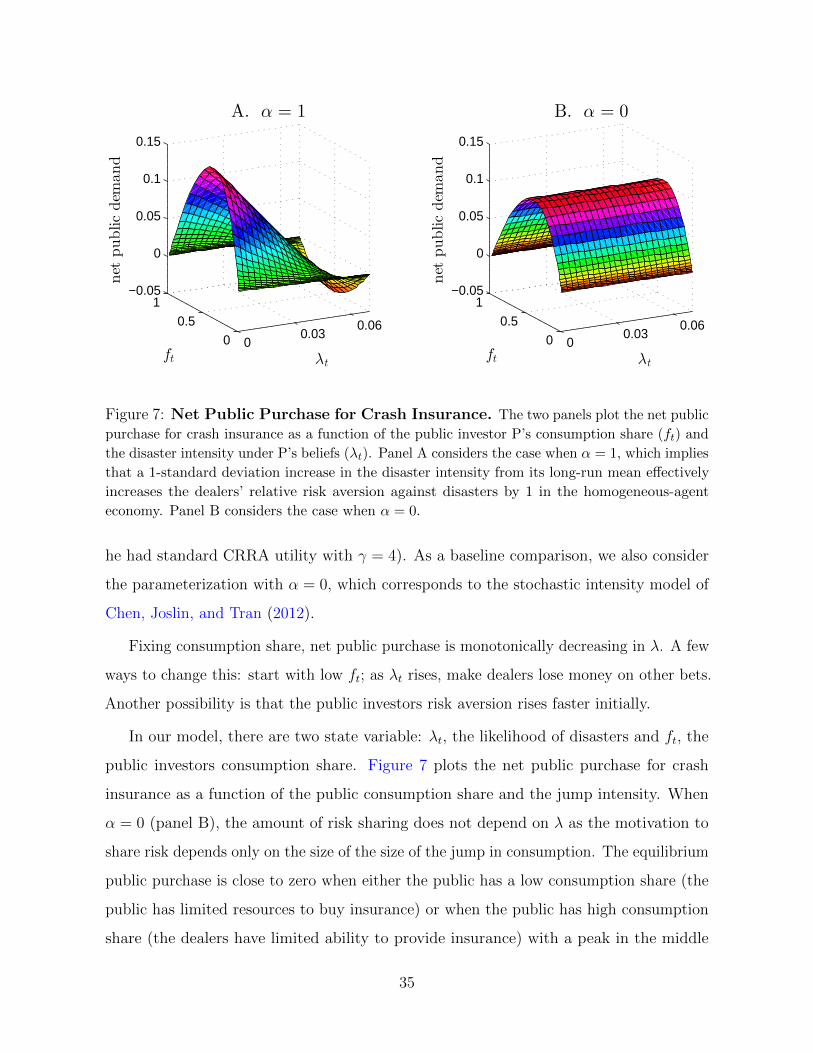
00.03

0.060

0.51

−0.05

0

0.05

0.1

0.15

λt

A. α = 1

ft

net

publicdem

and

00.03

0.060

0.51

−0.05

0

0.05

0.1

0.15

λt

B. α = 0

ft

net

publicdem

and

Figure 7: Net Public Purchase for Crash Insurance. The two panels plot the net public

purchase for crash insurance as a function of the public investor P’s consumption share (ft) and

the disaster intensity under P’s beliefs (λt). Panel A considers the case when α = 1, which implies

that a 1-standard deviation increase in the disaster intensity from its long-run mean effectively

increases the dealers’ relative risk aversion against disasters by 1 in the homogeneous-agent

economy. Panel B considers the case when α = 0.

he had standard CRRA utility with γ = 4). As a baseline comparison, we also consider

the parameterization with α = 0, which corresponds to the stochastic intensity model of

Chen, Joslin, and Tran (2012).

Fixing consumption share, net public purchase is monotonically decreasing in λ. A few

ways to change this: start with low ft; as λt rises, make dealers lose money on other bets.

Another possibility is that the public investors risk aversion rises faster initially.

In our model, there are two state variable: λt, the likelihood of disasters and ft, the

public investors consumption share. Figure 7 plots the net public purchase for crash

insurance as a function of the public consumption share and the jump intensity. When

α = 0 (panel B), the amount of risk sharing does not depend on λ as the motivation to

share risk depends only on the size of the size of the jump in consumption. The equilibrium

public purchase is close to zero when either the public has a low consumption share (the

public has limited resources to buy insurance) or when the public has high consumption

share (the dealers have limited ability to provide insurance) with a peak in the middle

35

0

0.03

0.06

0

0.5

10

10

20

30

λt

A. α = 1

ft

λQ t/λ

t

0

0.03

0.06

0

0.5

10

2

4

6

8

λt

B. α = 0

ft

λQ t/λ

t

Figure 8: Disaster Risk Premium. The two panels plot the conditional disaster risk

premium as a function of the public investor P’s consumption share (ft) and the disaster intensity

under P’s beliefs (λt). Panel A considers the case when α = 1. Panel B considers the case when

α = 0. Again, α = 1 means that a 1-standard deviation increase in the disaster intensity from its

long-run mean effectively increases the dealers’ relative risk aversion against disasters by 1 in the

homogeneous-agent economy.

where the public and dealers share a lot of risks. In contrasts, Panel B shows that when the

dealers have time-varying aversion to jump risks, the relationship is much more complex.

For low levels of the intensity the patterns is the same as before since the dealers are

as willing (or even more willing) to sell crash insurance. However, as λ rises, the clears

become more averse to jump risk and less willing to provide insurance. When the intensity

becomes high enough, the dealers become so averse to jump risk that they even begin to

become buyers of insurance rather than sellers.

Figure 8 plots the jump risk premium, as measured by λQ/λ, as a function of the

public consumption share and the jump intensity. In the case of α = 0, the jump risk

premium rises as there are fewer dealers to hold the jump risks. When α = 1, the jump

risk premium falls as there are more dealers when λ is low. When λ is high enough, this

relationship reverses and the premium rises as there are more dealers. The reason for this

is that as λ rises, the dealers become more risk averse and eventually demand a higher

premium than the public; this relation can be seen be following the curve with ft = 0,

36

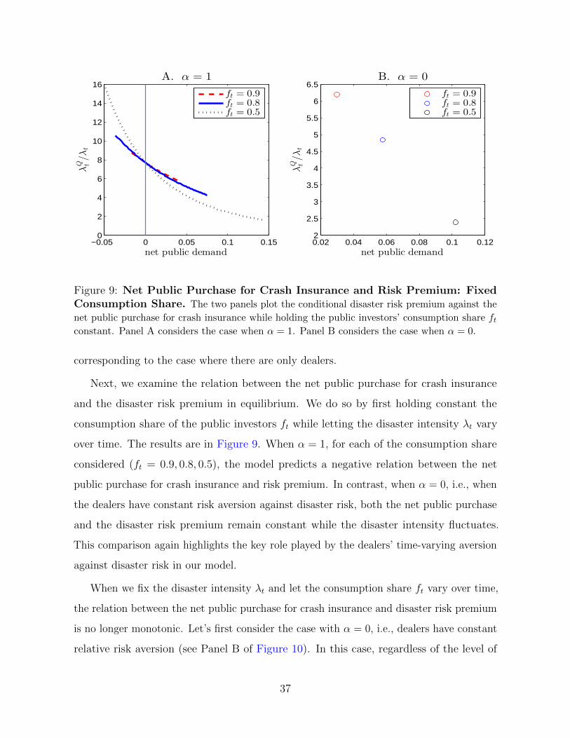
−0.05 0 0.05 0.1 0.150

2

4

6

8

10

12

14

16

net public demand

λQ t/λ

tA. α = 1

ft = 0.9ft = 0.8ft = 0.5

0.02 0.04 0.06 0.08 0.1 0.122

2.5

3

3.5

4

4.5

5

5.5

6

6.5

net public demand

λQ t/λ

t

B. α = 0

ft = 0.9ft = 0.8ft = 0.5

Figure 9: Net Public Purchase for Crash Insurance and Risk Premium: FixedConsumption Share. The two panels plot the conditional disaster risk premium against the

net public purchase for crash insurance while holding the public investors’ consumption share ftconstant. Panel A considers the case when α = 1. Panel B considers the case when α = 0.

corresponding to the case where there are only dealers.

Next, we examine the relation between the net public purchase for crash insurance

and the disaster risk premium in equilibrium. We do so by first holding constant the

consumption share of the public investors ft while letting the disaster intensity λt vary

over time. The results are in Figure 9. When α = 1, for each of the consumption share

considered (ft = 0.9, 0.8, 0.5), the model predicts a negative relation between the net

public purchase for crash insurance and risk premium. In contrast, when α = 0, i.e., when

the dealers have constant risk aversion against disaster risk, both the net public purchase

and the disaster risk premium remain constant while the disaster intensity fluctuates.

This comparison again highlights the key role played by the dealers’ time-varying aversion

against disaster risk in our model.

When we fix the disaster intensity λt and let the consumption share ft vary over time,

the relation between the net public purchase for crash insurance and disaster risk premium

is no longer monotonic. Let’s first consider the case with α = 0, i.e., dealers have constant

relative risk aversion (see Panel B of Figure 10). In this case, regardless of the level of

37

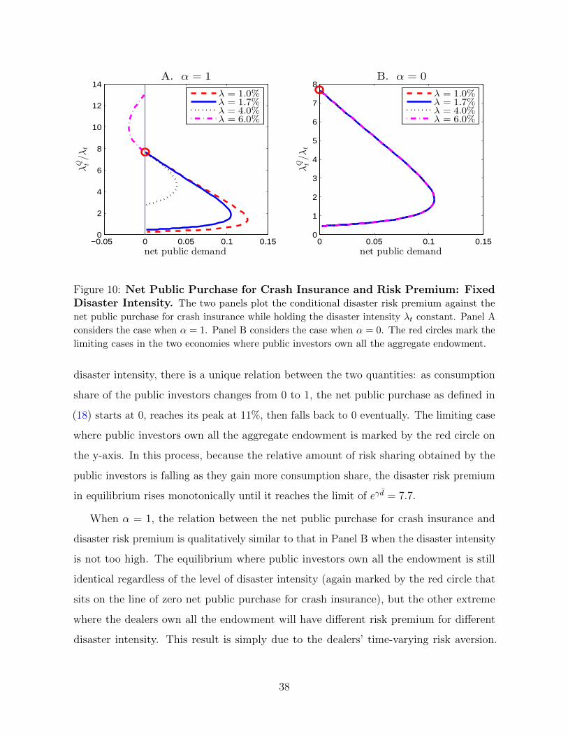
−0.05 0 0.05 0.1 0.150

2

4

6

8

10

12

14

net public demand

λQ t/λ

tA. α = 1

λ = 1.0%λ = 1.7%λ = 4.0%λ = 6.0%

0 0.05 0.1 0.150

1

2

3

4

5

6

7

8

net public demand

λQ t/λ

t

B. α = 0

λ = 1.0%λ = 1.7%λ = 4.0%λ = 6.0%

Figure 10: Net Public Purchase for Crash Insurance and Risk Premium: FixedDisaster Intensity. The two panels plot the conditional disaster risk premium against the

net public purchase for crash insurance while holding the disaster intensity λt constant. Panel A

considers the case when α = 1. Panel B considers the case when α = 0. The red circles mark the

limiting cases in the two economies where public investors own all the aggregate endowment.

disaster intensity, there is a unique relation between the two quantities: as consumption

share of the public investors changes from 0 to 1, the net public purchase as defined in

(18) starts at 0, reaches its peak at 11%, then falls back to 0 eventually. The limiting case

where public investors own all the aggregate endowment is marked by the red circle on

the y-axis. In this process, because the relative amount of risk sharing obtained by the

public investors is falling as they gain more consumption share, the disaster risk premium

in equilibrium rises monotonically until it reaches the limit of eγd = 7.7.

When α = 1, the relation between the net public purchase for crash insurance and

disaster risk premium is qualitatively similar to that in Panel B when the disaster intensity

is not too high. The equilibrium where public investors own all the endowment is still

identical regardless of the level of disaster intensity (again marked by the red circle that

sits on the line of zero net public purchase for crash insurance), but the other extreme

where the dealers own all the endowment will have different risk premium for different

disaster intensity. This result is simply due to the dealers’ time-varying risk aversion.

38

When λt is sufficiently high, the dealers can become so averse to disaster risk that, despite

of their optimist beliefs about the chances of disasters, they still demand a higher premium

than the public investors would. For this reason, when λt is sufficiently high, the net

public purchase for crash insurance turns negative, i.e., public investors are now insuring

the dealers against disasters, and the disaster risk premium in the economy exceeds the

highest level in the case with constant risk aversion.

While Figure 10 suggests that variation in consumption share can by itself generate

either positive or negative relation between net public purchase for crash insurance and

the risk premium, this channel is likely too weak in the time series. This is because the

consumption share moves slowly outside disasters. In contrast, because disaster intensity

is relatively volatile, the negative relation identified in Figure 9 will be tend to dominate

in the time series.

4 Extension

Our main model presented in Section 3.2 captures a number of the key features we have

found in the data. In particular, the model captures the fact that when equilibrium public

buying is low, risk premia may be high as this may correspond to time when dealers are

(or act as if they are) more risk averse. However, as in Chen, Joslin, and Tran (2012),

wealth moves slowly between the public sector and dealers outside of disasters and only

through the crash insurance premiums. In this section, we generalize our main model to

account for more general time variation in the relative wealth of the public and dealers.

Consider the case where public and dealers not only view the disaster events differently,

but also disagree about the future path of the likelihood of disasters. Specifically, consider

the more general form of (12) where

dPDdPP

= ρNte(1−ρ)∫ t0 λsds × e−

∫ s0 θsdW

λs −∫ t0 θ

2sds. (19)

and θs is some process satisfying Novikov’s condition. For example, with an appropriate

39

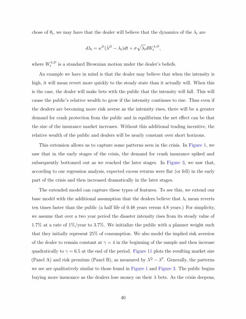
chose of θt, we may have that the dealer will believe that the dynamics of the λt are

dλt = κD(λD − λt)dt+ σ√λtdW

λ,Dt ,

where W λ,Dt is a standard Brownian motion under the dealer’s beliefs.

An example we have in mind is that the dealer may believe that when the intensity is

high, it will mean revert more quickly to the steady state than it actually will. When this

is the case, the dealer will make bets with the public that the intensity will fall. This will

cause the public’s relative wealth to grow if the intensity continues to rise. Thus even if

the dealers are becoming more risk averse as the intensity rises, there will be a greater

demand for crash protection from the public and in equilibrium the net effect can be that

the size of the insurance market increases. Without this additional trading incentive, the

relative wealth of the public and dealers will be nearly constant over short horizons.

This extension allows us to capture some patterns seen in the crisis. In Figure 1, we

saw that in the early stages of the crisis, the demand for crash insurance spiked and

subsequently bottomed out as we reached the later stages. In Figure 3, we saw that,

according to our regression analysis, expected excess returns were flat (or fell) in the early

part of the crisis and then increased dramatically in the later stages.

The extended model can capture these types of features. To see this, we extend our

base model with the additional assumption that the dealers believe that λt mean reverts

ten times faster than the public (a half life of 0.48 years versus 4.8 years.) For simplicity,

we assume that over a two year period the disaster intensity rises from its steady value of

1.7% at a rate of 1%/year to 3.7%. We initialize the public with a planner weight such

that they initially represent 25% of consumption. We also model the implied risk aversion

of the dealer to remain constant at γ = 4 in the beginning of the sample and then increase

quadratically to γ = 6.5 at the end of the period. Figure 11 plots the resulting market size

(Panel A) and risk premium (Panel B), as measured by λQ − λP. Generally, the patterns

we see are qualitatively similar to those found in Figure 1 and Figure 3. The public begins

buying more insurance as the dealers lose money on their λ bets. As the crisis deepens,

40

0 0.5 1 1.5 2−0.02

−0.01

0

0.01

0.02

0.03Net

Public

Holding

Time (years)

A. Market Size

0 0.5 1 1.5 24

5

6

7

8

9

10

λQ/λ

P

Time (years)

B. Risk premium

Figure 11: Dealer constraint and derivative supply. This figure plots the equilibrium

holding of crash insurance by the public investors (Panel A) and disaster risk premium (Panel B)

for a hypothetical history where the intensity rises from 1.7% to 3.7% over a two year period.

The public has an initial consumption fraction of 0.25. The dealer’s relative risk aversion is

initially γ = 4 and then rises in the second half quadratically to γ = 6.5.

the dealers start to become very risk averse and the market dries up to the point where

the dealers even become buyers of protection. Across this time period, the risk premium

at first increases very slowly until the dealers are no longer willing to hold the risk and

the premium begins to increase rapidly.

5 Conclusion

The options market is an integral part of the risk sharing mechanism in the economy,

where the risk bearing capacity of the intermediaries play a key role in determining not

only the prices and equilibrium demand for options, but also the risk premium in the

aggregate economy.

We provide evidence that measures of the amount of trading between public investors

and financial intermediaries on DOTM SPX puts have strong predictive power for future

market excess returns. The PNBO volume of public investors are negatively associated

41

with future market returns up to the 4 months ahead. PNBO are negatively associated

with the expensiveness of the DOTM index puts and positively associated with the change

in broker-dealer leverage. Moreover, the information that PNBO contains about the

market risk premium is not captured by the standard financial and macro variables. This

result is consistent with the prediction of the intermediary-based asset pricing models in

that time-varying intermediary constraints can drive the aggregate risk premium.

To explain these findings, we build a general equilibrium model of a market for the

crash insurance market, which captures the dynamic relation between the net demand

by public investors and the disaster risk premium. As dealers become more constrained

and averse to disaster risk when the probability of disaster risk is high, their risk sharing

capacity is reduced, causing the equilibrium net public purchase for crash insurance to fall

and the disaster risk premium to rise.

42

References

Adrian, Tobias, and Nina Boyarchenko, 2012, Intermediary leverage cycles and financial

stability, Staff reports, Federal Reserve Bank of New York.

Adrian, Tobias, Erkko Etula, and Tyler Muir, 2012, Financial intermediaries and the

cross-section of asset returns, Working Paper.

Adrian, Tobias, Emanuel Moench, and Hyun Song Shin, 2010, Financial intermediation,

asset prices, and macroeconomic dynamics, Staff Reports 422 Federal Reserve Bank of

New York.

Adrian, Tobias, and Hyun Song Shin, 2010, Liquidity and leverage, Journal of Financial

Intermediation 19, 418–437.

Bates, David S., 2008, The market for crash risk, Journal of Economic Dynamics and

Control 32.

Bollerslev, Tim, George Tauchen, and Hao Zhou, 2009, Expected stock returns and variance

risk premia, Review of Financial Studies 22, 4463–4492.

Brunnermeier, Markus K., and Lasse Heje Pedersen, 2009, Market liquidity and funding

liquidity, Review of Financial Studies 22, 2201–2238.

Brunnermeier, Markus K., and Yuliy Sannikov, 2013, A macroeconomic model with a

financial sector, Working Paper, Princeton University.

Buraschi, Andrea, and Alexei Jiltsov, 2006, Model uncertainty and option markets with

heterogeneous beliefs, Journal of Finance 61, 2841–2897.

Chen, Hui, Scott Joslin, and Ngoc-Khanh Tran, 2012, Rare disasters and risk sharing with

heterogeneous beliefs, Review of Financial Studies 25, 2189–2224.

Cheng, Ing-Haw, Andrei Kirilenko, and Wei Xiong, 2012, Convective risk flows in com-

modity futures markets, NBER Working Papers 17921, National Bureau of Economic

Research, Inc.

43

Cochrane, John H., 2011, Presidential address: Discount rates, Journal of Finance 66,

1047–1108.

Cox, John C., and Chifu Huang, 1989, Optimum consumption and portfolio policies when

asset prices follow a diffusion process, Journal of Economic Theory 49, 33–83.

Garleanu, Nicolae, Lasse Heje Pedersen, and Allen M. Poteshman, 2009, Demand-based

option pricing, Review of Financial Studies 22, 4259–4299.

Geanakoplos, John, 2009, The leverage cycle, Cowles Foundation Discussion Papers 1715

Cowles Foundation for Research in Economics, Yale University.

Gertler, Mark, and Nobuhiro Kiyotaki, 2013, Banking, liquidity and bank runs in an

infinite-horizon economy, NBER Working Papers.

Gromb, Denis, and Dimitri Vayanos, 2002, Equilibrium and welfare in markets with

financially constrained arbitrageurs, Journal of Financial Economics 66, 361–407.

Hansen, Lars Peter, and Robert J Hodrick, 1980, Forward exchange rates as optimal

predictors of future spot rates: An econometric analysis, Journal of Political Economy

88, 829–53.

Hansen, P.R., and A. Timmermann, 2012, Choice of sample split in out-of-sample forecast

evaluation, Working Paper, Stanford University.

He, Zhiguo, and Arvind Krishnamurhty, 2012, Intermediary asset pricing, Forthcoming,

American Economic Review.

Hong, Harrison, and Motohiro Yogo, 2012, What does futures market interest tell us about

the macroeconomy and asset prices?, Journal of Financial Economics 105, 473 – 490.

Kelly, Bryan, 2012, Tail risk and asset prices, Working Paper, University of Chicago Booth

School of Business.

Lettau, Martin, and Sydney Ludvigson, 2001, Resurrecting the (C)CAPM: a cross-sectional

test when risk premia are time-varying, Journal of Political Economy 109, 1238–1287.

44

Lo, Andrew, 2001, Risk management for hedge funds: Introduction and overview, Financial

Analysts Journal 57, 16–33.

Longstaff, Francis A., and Jiang Wang, 2012, Asset pricing and the credit market, Review

of Financial Studies 25, 3169–3215.

Makarov, Igor, and Guillaume Plantin, 2011, Rewarding trading skills without inducing

gambling, Working Paper, London Business School.

Malliaris, Steven, and Hongjun Yan, 2010, Reputation Concerns and Slow-Moving Capital,

Working Paper, Yale University.

Pan, Jun, and Allen Poteshman, 2006, The information in option volume for future stock

prices, Review of Financial Studies 19, 871–908.

Welch, Ivo, and Amit Goyal, 2008, A comprehensive look at the empirical performance of

equity premium prediction, Review of Financial Studies 21, 1455–1508.

45