Embed Size (px)
Citation preview

1
Demand for Money in Papua New Guinea
Tanu Irau November 20, 2014
Abstract
Time series data for the period 1978:Q1 to 2010:Q4 was analyzed to estimate the
demand for real broad money (M3) in Papua New Guinea (PNG) with the aim of establishing its
determinants and the function’s stability. As most time series data are non-stationary, which
potentially may lead to the spurious regression problem, individual data series were tested for
unit roots using the Augmented Dickey Fuller (ADF) and Kwiatkowski-Phillips-Schmidt-Shin
(KPSS) tests. The tests showed that variables defined in levels are non-stationary but are
stationary in first differences, i.e. integrated of order one.
The Engel-Granger method of co-integration and error correction was adopted to model
the demand for money in PNG. It was found that there is a long-run co-integrating relationship
between real broad money, income, price, financial innovation and the exchange rate. Demand
for money is determined by income, financial innovation and the US$/kina exchange rate in the
long-run. Interest rate was found to be insignificant in explaining real money demand in PNG in
the long-run. Income and price (inflation) influence the demand for money in the short-run.

2
Table of Contents
1.0 Introduction ...................................................................................................................... 3
2.0 Theories of Money Demand............................................................................................. 4
3.0 Money Demand Studies in Papua New Guinea.............................................................. 5
4.0 Empirics............................................................................................................................. 7
4.1 Data ................................................................................................................................ 7
4.2 Unit Root Test ................................................................................................................ 8
4.3 Co-integration and Error Correction ........................................................................... 10
5.0 Results and Interpretation ............................................................................................ 15
5.1 Long-Run Elasticity .................................................................................................... 15
5.2 Short-run Dynamics .................................................................................................... 16
6.0 Conclusion ...................................................................................................................... 17
7.0 Appendix.......................................................................................................................... 18
References..................................................................................................................................... 23

3
1.0 Introduction
A stable money demand function is necessary for monetary policy and a useful
instrument for macroeconomic policy. It is therefore essential that policy makers are
mindful of the properties of the money demand function and its linkage to the rest of
the economy when formulating policy. Given the important link of money demand to
the rest of the economy, it has been studied extensively at both the theoretical and
empirical levels in many countries.
The study of money demand seeks to establish whether the function is
stable for the concerned economy. If the function is stable then its application in
monetary policy can exert a predictable influence on the real economy because “the
quantity of money is predictably related to a set of variables linking money to the real
sector of the economy” (Judd & Scadding, 1982). A stable money demand function
hence becomes necessary for monetary policy formulation and a useful instrument of
macroeconomic policy.
Though economic theory does not provide a precise mathematical function for
the demand for money, there is a general consensus that the log-linear version is the
appropriate functional form (Zarembka, 1968). The general specification of the model
and the selection of variables relate some monetary aggregate to a scale variable and
an opportunity cost variable.
This analysis is motivated by the following observations. Firstly, the Bank of
Papua New Guinea (BPNG) formulates and implements monetary policy in the
absence of an empirically tested money demand function. Secondly, the demand for
money is important in determining the effectiveness of fiscal policy in changing the
level of income (Dornbusch & Fisher, 1981). Thirdly, apart from a piece in the
International Monetary Fund (IMF) 1993 Article IV Consultation report, Kanari’s (1998)
in-house discussion paper and Kannapiran (2001), there is no other published work on
money demand in PNG.
The objective of the paper is to examine the determinants and stability of the
money demand function for PNG.
The paper proceeds as follows. Theories of money demand are briefly covered
in section 2. Section 3 provides a review of money demand analysis done for PNG. In
section 4, data, methodology and empirics are presented, while results are discussed
in section 5. Section 6 concludes the paper and highlights areas for further research.

4
2.0 Theories of Money Demand
The Classical Theorists’ “equation of exchange” relates the amount of money
in circulation in an economy to the number of transactions and the average price level
in a given period. This is done through a proportionality factor called the transactions
velocity of circulation; MV = PT, where M is total quantity of money, V is velocity1, P is
the price level and T being the number of transactions. A feature of the quantity theory
of money is that interest rates do not influence the demand for money (Mishkin, 2007).
The equation of exchange is an identity where it does not say anything about the
direction of change in income when there is a change in the supply of money.
According to Fisher (1911), velocity is determined by the institutions and
technological features in an economy that affect the way individuals conduct
transactions and it is assumed to be constant in the short-run. This is because it takes
time for institutions and technology to change. It is also assumed that income is at the
full employment level and is also constant. The quantity theory of money implies that
the demand for money is determined by the number of transactions generated by the
level of nominal income (price x income) and the institutions and technology in the
economy. Classical economists believed in price flexibility whereby if income is
relatively fixed in the short-run then money and price are proportional. This means that
an increase in the money supply only leads to an increase in the price level and
interest rate does not influence money demand.
The Keynesian approach that underpins the traditional IS-LM2 framework,
postulates that the demand for money is a special case where individuals hold money
for transaction, precautionary and speculative reasons. The transaction motive stems
from the emphasis that money is a medium of exchange and has a stable relationship
to the level of income. This is because payments and receipts do not necessarily occur
simultaneously. The precautionary reason creates demand for money when individuals
are unsure of the payments they might want, or have to make; thus creating a fallback
plan for unscheduled expenditure for unforeseen situations. According to Keynes, the
speculative motive is really the “liquidity preference theory of money”, where
1 Velocity is defined as the average number of times per year (turnover) that a kina is spent buying the total amount of goods and services produced in the economy. In other words, it is total spending (Price x Income) divided by the quantity of money, M, i.e: = 𝑃𝑃𝑃𝑃
𝑀𝑀.
2 A model often used as an extremely simple example of general equilibrium in macroeconomics. The IS curve shows the combinations of income (y) and interest rate (r) at which savings and investment are equal. The LM curve shows the combinations of y and r at which the supply of and demand to hold money are in equilibrium. Where the IS and LM curves intersect, both the market for goods and the market for money balances are simultaneously in equilibrium.

5
uncertainty about the future influences the demand for money. The focus was to
identify a link between money and interest rates as interest rate matters in the demand
for money – the opportunity cost of holding money. The basic Keynesian money
demand function is normally stated as:
�𝑀𝑀𝑃𝑃� = 𝑓𝑓(𝑌𝑌, 𝑖𝑖) (1)
where real money demand �𝑀𝑀𝑃𝑃� is a function of income (Y) and interest rate (i).
According to the Keynesians, velocity depends on the interest rate and when it
fluctuates a lot so does velocity. For instance, an increase in the interest rate would
lead to a decline in money holdings because it would be less profitable to hold money.
Applying the theory of asset demand, Friedman’s (1956) modern quantity theory
postulates that the demand for money is influenced by the same factors that influence
the demand for any other asset. This is expressed as:
�𝑀𝑀𝑑𝑑
𝑃𝑃� = 𝑓𝑓�𝑌𝑌𝑝𝑝, 𝑟𝑟𝑏𝑏 − 𝑟𝑟𝑚𝑚, 𝑟𝑟𝑒𝑒 − 𝑟𝑟𝑚𝑚,𝜋𝜋𝑒𝑒 − 𝑟𝑟𝑚𝑚� (2)
where
𝑌𝑌𝑝𝑝 is permanent income
𝑟𝑟𝑏𝑏 is expected return on bonds
𝑟𝑟𝑚𝑚 expected return on money
𝑟𝑟𝑒𝑒 is expected return on equity
𝜋𝜋𝑒𝑒 is expected inflation rate
The modern quantity theory of money basically indicates that the demand for
money should be a function of resources (wealth) and expected returns on other
assets relative to expected return on money. All the coefficients of the determinants of
real money demand are expected to be negative except for income, 𝑌𝑌𝑝𝑝.
3.0 Money Demand Studies in Papua New Guinea
A money demand function for PNG was first estimated by the IMF; using
quarterly data for the period 1980 to 1990. Based on the conventional partial

6
adjustment model3, money demand was specified as a log-linear function of real GDP,
the inflation rate (𝜋𝜋𝑡𝑡), financial innovation4 and real money lagged one period. The
scale variable for the analysis was the real GDP, a proxy for transactions relating to
economic activity. The inflation rate was used as a proxy for the opportunity cost of
holding money. Inaccessibility to financial services in an underdeveloped financial
market is seen to be a reason why individuals hold money, so financial innovation was
used to capture this effect5 (BPNG, 2007).
The IMF study established that 98.5% of the variation in the demand for real
money balances in PNG is explained by model. The signs on the coefficients were as
expected with real money demand positively related to real GDP and money demand
in the previous period, and inversely related to inflation and financial innovation. An
increase in income results in an increase in the demand for money, all else held
constant. Likewise, an increase in money demand in the previous period will lead to an
increase in the demand for money in the current period, ceteris paribus. The increase
in economic activity requires higher levels of money holdings to facilitate these
transactions, hence an increase in the demand for money in the current period. With
inflation, money loses its purchasing power and increases the cost of holding it thereby
leading to a contraction in money demand. Financial innovation is expected to cause a
decline in demand for money, everything else held constant.
An in-house discussion paper by Kanari (1998) followed the IMF’s partial
adjustment model with an increased number of observations; 1978Q1 – 1997Q4 as
the sample period. The results were similar to the IMF’s.
Kannapiran (2001) provided a brief review of earlier research on money demand
which gave the basis for the estimated money demand function for PNG. He cited a
number of money demand studies done for developed and developing countries.
Quarterly data for the period 1975 to 1995 were used and the error correction
framework was applied as it has proven to be a successful tool in applied money
demand research (Sriram, 1999). The study aimed to establish the empirical basis for
the conduct of monetary policy by the BPNG. It was found that the demand for money
was influenced by real GDP, inflation and money demand in the previous period, while
interest rate was found to be insignificant.
3 See Appendix for a brief discussion on the partial adjustment model.4 Financial innovation is defined as the ratio of currency in circulation (cic) to total deposits at the commercial banks. Tseng and Corker’s (1991) study on SEACEN4 member countries confirmed that financial innovation does influence money demand.5 Hye (2009) found that financial innovation (defined as the ratio of narrow money and broad money) had significant effect both in the short and long run in the demand for money in Pakistan.

7
Kannapiran (2001) established that 82% of the variation in the demand for money in
PNG was explained by the model. The signs of all the coefficients were as expected
and were significant at the 1 percent level of significance with the exception of the
interest rate variable. The level of income was found to be the main determinant of the
demand for money with an income elasticity of 0.21. According to the Kannapiran
study, money demand was stable during the period 1975-1995. However, the study
was done before the financial sector reforms in 2000 and since then changes have
taken place which warrants a re-assessment of the money demand function.
4.0 Empirics
4.1 Data
This analysis is based on quarterly data for the period 1978-2010, sourced from
various issues of BPNG’s Quarterly Economic Bulletin (QEB), the Department of
Treasury and the National Statistical Office (NSO). The dependent variable is real
broad money (M3*)6. The scale variable is real GDP while the Consumer Price Index
(CPI) and 182-day weighted average Treasury bill rate are proxies for the opportunity
cost variable. Mundell (1963) argued that in addition to interest rate and income, the
demand for money is likely to depend on the exchange rate, hence the inclusion of the
US/kina exchange rate to see if this is the case in PNG. The coefficient for the
exchange rate is expected to be either positive or negative. Arango and Nadiri (1981)
argue that a depreciation of the domestic currency (an appreciation of foreign
currency) increases the domestic currency value of foreign securities held by domestic
residents. If this increase is perceived as an increase in wealth, the demand for
domestic currency by domestic residents could increase, hence a positive coefficient.
In contrast, Bahmani-Oskooee and Poorheydarian (1990) argued that when the
domestic currency depreciates, there could be expectation of further depreciation. This
could induce the public to increase holdings of foreign currency by drawing down their
holdings of domestic money.
Following the IMF model, the ratio of currency in circulation to total deposits
(placed at commercial banks) is included as a proxy for financial innovation. An
alternative proxy for financial innovation is to include a trend variable in the model but
this is not considered in this analysis. It should be noted that PNG’s NSO only
6 Broad money supply (M3*) in PNG comprises narrow money (M1*) plus quasi-money.

8
compiles annual GDP and so the quarterly series was derived from the annual series
by employing a simple interpolation method (frequency conversion from low to high7 in
Eviews. Tables A1 and A2 in the Appendix present the descriptive statistics and the
results of correlation analysis. The correlation analysis shows that real broad money is
related to the selected explanatory variables. With the exception of the interest rate
variable, the correlations are statistically significant at the 1% level of significance.
4.2 Unit Root Test8
Before testing for no co-integration, unit root test is undertaken to make certain
that the variables are integrated of the same order, in this case integrated of order
one, I(1). Unit root tests such as the ADF, Phillips-Perron and KPSS9 are now a
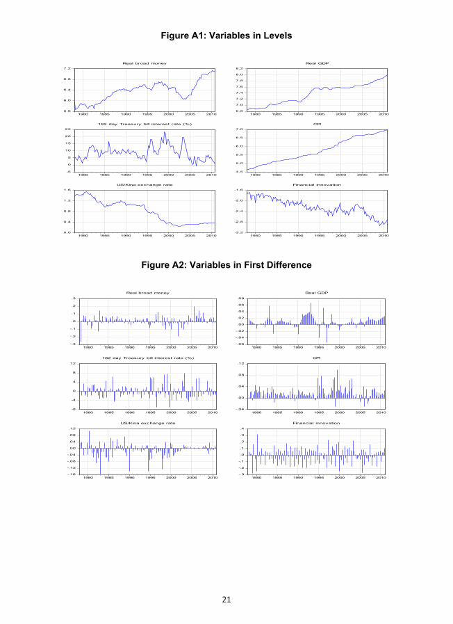
standard procedure for testing for the order of integration of the variables. Figures A1
and A2 (see Appendix) plot the variables defined in levels and first differences,
respectively, as an informal test for stationarity (Takaendesa, 2006).
The ADF tests are based on the following autoregressive (AR) models:
∆𝑥𝑥𝑡𝑡 = 𝜇𝜇 + 𝜌𝜌𝑥𝑥𝑡𝑡−1 + ∑ 𝜃𝜃𝑖𝑖∆𝑥𝑥𝑡𝑡−𝑖𝑖𝑘𝑘𝑖𝑖=1 + 𝜀𝜀𝑡𝑡 (3)
∆𝑥𝑥𝑡𝑡 = 𝜇𝜇 + 𝛿𝛿𝛿𝛿 + 𝜌𝜌𝑥𝑥𝑡𝑡−1 + ∑ 𝜃𝜃𝑖𝑖∆𝑥𝑥𝑡𝑡−𝑖𝑖𝑘𝑘𝑖𝑖=1 + 𝜀𝜀𝑡𝑡 (4)
∆𝑥𝑥𝑡𝑡 = 𝜌𝜌𝑥𝑥𝑡𝑡−1 + ∑ 𝜃𝜃𝑖𝑖∆𝑥𝑥𝑡𝑡−𝑖𝑖𝑘𝑘𝑖𝑖=1 + 𝜀𝜀𝑡𝑡 (5)
where k = the number of lags selected and t = time period
The null hypothesis of a unit root is rejected in favor of the alternative of level
stationary if rho (𝜌𝜌) in equations 3, 4 and 5 are significantly different from zero. For this
study, the ADF tests in levels use equation (4) because trends are apparent except for
the interest rate series while equation (3) is used for the first differences. ADF unit root
7 This method fits a quadratic polynomial for each observation of the low frequency series, and then uses this polynomial to fill in all observations of the high frequency series associated with the period. The quadratic polynomial is formed by taking sets of three adjacent points from the source series and fitting a quadratic so that the average of the high frequency points matches the low frequency data actually observed. For most points, one point before and one point after the period currently being interpolated are used to provide the three points. For end points, the two periods are both taken from the one side where data is available (see EViews User’s Guide I, pp. 119).8 See Appendix for a simplified ADF procedure.9 The ADF test often suffers from low power. That is, probability that they lead to rejecting the null hypothesis of unit root is low hence leading to the conclusion that there are unit roots where there are not.The KPSS test is a way to circumvent this problem is to test the null hypothesis that there is no unit root against the alternative that there is a unit root.

9
test for data defined in first differences excludes the time trend as no trend is apparent.
The computed ADF test statistics for the levels and first differences are presented in
Table 1. The results indicate that the variables defined in levels10, where the null
hypothesis of unit root (non-stationary) cannot be rejected at the 5% level of
significance, but the null that their first differences have unit roots is clearly rejected.
Therefore, it is concluded that the variables defined in levels are integrated of order
one, I(1) and can be modeled with the vector auto-regression (VAR) if the co-
integration test does not reject the null hypothesis of no co-integration. An error
correction (or VEC approach) would be appropriate if the variables are found to be
non-stationary and co-integrated. The results from the KPPS unit root test confirm that
variables in levels are non-stationary but stationary in first difference, at the 1% level of
significance.
Table 1: Unit Root Test
Variable
Augmented Dickey-Fuller test
Kwiatkowski-Phillips-Schmidt-Shin (KPSS)
test statistic
Level 1st
DifferenceLevel 1st
Differencelrm3 -1.28 -7.06*** 0.140 0.141lry -2.20 -8.13*** 0.088 0.057lp -1.50 -9.24*** 0.214 0.128fin -2.55 -6.19*** 0.176 0.076int -3.25* -8.09*** 0.184 0.111
xr -1.16 -11.10*** 0.118 0.141
Critical Values11
1% -3.48 -4.03 0.216 0.7395% -2.88 -3.44 0.146 0.46310% -2.58 -3.15 0.119 0.347
Note:*** 1% level of significance** 5% level of significance* 10% level of significance
10 Data transformed into logarithms only smooth the series but does not solve for stationarity.11 The critical values for the ADF test are taken from R. Davidson and J.G MacKinnon (1993), Estimation and Inference in Econometrics, New York, Oxford University Press, p. 708. Critical values for the KPPS test are from *Kwiatkowski-Phillips-Schmidt-Shin (1992, Table 1).
10
The variables in Table 1 are defined as:
lrm3: natural log of real broad money
lry: natural log of real gross domestic product
lp: natural log of consumer price index
fin: financial innovation (cic12/deposits)
int: weighted average interest rate on 182-day Treasury bills (%)
xr: kina exchange rate against the US dollar (USD/PGK)
4.3 Co-integration and Error Correction
Developments in both the theoretical and technological levels have led to the
concept of co-integration and error-correction models (ECM) becoming increasingly
popular as they appear to provide better results. Co-integration deals with the
relationships amongst a set of non-stationary time series data. If a set of variables are
co-integrated, the effects of a shock to one variable spreads to the others, possibly
with time lags, so as to preserve a long-run relationship between the variables. The
ECMs have proven to be one of the most successful econometric tools in applied
money demand research. This type of formulation is a dynamic error-correction
representation in which the long-run equilibrium relationship between money and its
determinants is entrenched in an equation that captures short-run variation and
dynamics (Kole and Meade, 1995). The ECM is shown to contain information on both
the short and long-run properties of the model with disequilibria as a process of
adjustment to the long-run model.
To determine whether real money balance in PNG has a long-run equilibrium
relationship with the explanatory variables, the Engel and Granger (1987), often
referred to as the EG approach is adopted. As a starting point and following
Kannapiran (2001)13, the EG approach is used to estimate the basic Keynesian money
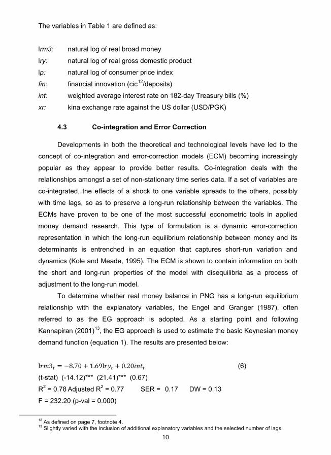
demand function (equation 1). The results are presented below:
l𝑟𝑟𝑟𝑟3𝑡𝑡 = −8.70 + 1.69l𝑟𝑟𝑟𝑟𝑡𝑡 + 0.20𝑖𝑖𝑖𝑖𝑖𝑖𝑡𝑡 (6)
(t-stat) (-14.12)*** (21.41)*** (0.67)
R2 = 0.78 Adjusted R2 = 0.77 SER = 0.17 DW = 0.13
F = 232.20 (p-val = 0.000)
12 As defined on page 7, footnote 4.13 Slightly varied with the inclusion of additional explanatory variables and the selected number of lags.

11
Note:
*** represents 1% level of significance
** represents 5% level of significance
* represents 10% significance level
The unit root test on the residual from equation (6) showed the following:
∆𝜀𝜀𝑡𝑡 = −0.06𝜀𝜀𝑡𝑡−1 + 0.06∆𝜀𝜀𝑡𝑡−1 (7)
(-2.09) (0.84)
The t-statistic for rho (𝜌𝜌) is equal to -2.09 in equation (7) is greater than the 1%,
5% and 10% critical values of -3.39, -2.76 and -2.45 respectively and therefore we fail
to reject the null hypothesis of no co-integration and conclude that equation (1) is a
non-co-integrating relationship. As such, the ECM cannot be applied. Since the null
hypothesis of no co-integration cannot be rejected, an alternate econometric model is
estimated where the long-run demand for real broad money is specified as:
l𝑟𝑟𝑚𝑚3𝑡𝑡 = 𝑎𝑎0 + 𝛼𝛼1l𝑟𝑟𝑦𝑦𝑡𝑡 + 𝛼𝛼2𝑖𝑖𝑖𝑖𝑖𝑖𝑡𝑡 + 𝛼𝛼3𝑓𝑓𝑖𝑖𝑖𝑖𝑡𝑡 + 𝛼𝛼4𝑥𝑥𝑟𝑟𝑡𝑡 + 𝑎𝑎5l𝑝𝑝𝑡𝑡 + 𝜀𝜀𝑡𝑡 (8)
The specified econometric model in equation (8) is a potential long-run co-
integrating relationship. If the residuals from the ordinary least squares (OLS)
regression (equation (8)) are found to be stationary, that is, 𝜀𝜀𝑡𝑡 ∽ 𝐼𝐼(0), (but only if each
of the underlying series is integrated of order 1, I(1) then it can be concluded that
equation (8) is a co-integrating relationship. This is estimated with the two-step Engel-
Granger method, where the residuals from the static regression, equation (8), is
included as an explanatory variable in equation (9), to determine the speed of
adjustment (𝜃𝜃) to its long-run equilibrium. The general error correction representation
of equation (8) is:
∆l𝑟𝑟𝑚𝑚3𝑡𝑡 =
𝜇𝜇 + 𝛿𝛿1l𝑟𝑟𝑦𝑦𝑡𝑡 + 𝛿𝛿2𝑖𝑖𝑖𝑖𝑖𝑖𝑡𝑡 + 𝛿𝛿3𝑓𝑓𝑖𝑖𝑖𝑖𝑡𝑡 + 𝛿𝛿4𝑥𝑥𝑟𝑟𝑡𝑡 + 𝛿𝛿5l𝑝𝑝𝑡𝑡 + ∑ 𝜑𝜑𝑖𝑖𝑘𝑘𝑖𝑖=1 ∆l𝑟𝑟𝑚𝑚3𝑡𝑡−𝑖𝑖 + ∑ 𝛾𝛾𝑖𝑖𝑘𝑘
𝑖𝑖=0 ∆l𝑟𝑟𝑦𝑦𝑡𝑡−𝑖𝑖 +
∑ 𝜗𝜗𝑖𝑖𝑘𝑘𝑖𝑖=0 ∆𝑖𝑖𝑖𝑖𝑖𝑖𝑡𝑡−𝑖𝑖 + ∑ 𝜔𝜔𝑖𝑖
𝑘𝑘𝑖𝑖=0 ∆𝑓𝑓𝑖𝑖𝑖𝑖𝑡𝑡−𝑖𝑖 + ∑ 𝜎𝜎𝑖𝑖𝑘𝑘
𝑖𝑖=0 ∆𝑥𝑥𝑟𝑟𝑡𝑡−𝑖𝑖 + ∑ 𝜏𝜏𝑖𝑖𝑘𝑘𝑖𝑖=0 ∆l𝑝𝑝𝑡𝑡−𝑖𝑖 − 𝜃𝜃𝐸𝐸𝐸𝐸𝑡𝑡−1 + 𝑢𝑢𝑡𝑡
(9)

12
where k = 1 – 4 lags
Table 1 shows the results of the long-run money demand relationships.
Table 1: Regression Results (long-run models)
Variable Model 1 Model 2 Model 3
𝑎𝑎0-4.291
(-3.729)***
-3.870
(-3.713)***
-2.876
(-2.980)***
l𝑟𝑟𝑦𝑦𝑡𝑡0.923
(6.267)***
0.950
(6.617)***
0.890
(5.986)***
𝑖𝑖𝑖𝑖𝑖𝑖𝑡𝑡0.597
(2.185)**
0.490
(2.042)**…..
𝑓𝑓𝑖𝑖𝑖𝑖𝑡𝑡-8.108
(-8.995)***
-8.208
(-9.191)***
-8.444
(-8.906)***
𝑥𝑥𝑟𝑟𝑡𝑡0.412
(3.444)***
0.319
(6.110)***
0.271
(2.652)***
l𝑝𝑝𝑡𝑡0.066
(0.857)…..
-0.009
(-0.135)
R2 0.873 0.872 0.868
Adjusted R2 0.868 -0.868 0.864
SER 0.132 0.132 0.134
F-statistic 173.530 217.148 209.500
AIC -1.161 -1.70 -1.139
SC -1.03 -1.126 -1.030
Residual-based Co-
integration test: rho (𝜌𝜌)-3.52 -3.50 -3.40
The results of the long-run models 1 and 2 have the expected signs on the
income, financial innovation and exchange rate but the opportunity cost variables have
the incorrect signs. As such these are discarded and model 3 is chosen as the

13
appropriate long-run model. The residual-based ADF unit root test for no co-integration
(model 3) showed the following results:
∆𝜀𝜀𝑡𝑡 = −0.25𝜀𝜀𝑡𝑡−1 − 0.33∆𝜀𝜀𝑡𝑡−1 (10)
(t-stat) (-3.40)*** (-4.05)***
For the selected long-run model (3), the value of rho in equation (10) is -3.40,
which is less than the critical value at the 1% level of significance (-3.39) and therefore
we reject the null hypothesis of no co-integration and conclude that equation (8) is
indeed a long-run co-integrating relationship. The results of the over-parameterized
general ECM representation (equation 9) are shown in the appendix (Table A3). A
parsimonious model is estimated after sequentially omitting the insignificant variables
and the results are shown in Table 2.
Table 2: Regression Results (parsimonious model)Variable Coefficient Std. Error t-Statistic Probability
l𝑟𝑟𝑦𝑦𝑡𝑡 0.01 0.00 6.99 0.000
∆𝑙𝑙𝑙𝑙𝑡𝑡 -1.24 0.20 -6.14 0.000
∆𝑙𝑙𝑙𝑙𝑡𝑡−2 -0.68 0.20 -3.40 0.001
𝐸𝐸𝐸𝐸𝑡𝑡−1 -0.09 0.03 -2.83 0.005
R2 0.327
Adjusted R2 0.311
SER 0.044
Diagnostic Tests
Serial Correlation
Breusch-Godfrey LM Test
AR(1)
AR(12)
Durbin-Watson
H0: no autocorrelation; H1: autocorrelation
F-stat = 0.859 Prob. F(1, 124) = 0.356 [fail to reject H0]
F-stat = 1.41 Prob. F(12, 113) = 0.335 [fail to reject H0]
2.160 [no autocorrelation]
Heteroskedasticity
Breusch-Pagan-Godfrey
(e2 = c dp dlry(-2) e(-1))
White
(e2 = c dp2 dlry(-2)2 e(-1)2)
H0: homoskedatsic; H1: heteroskedastic
F-stat = 0.373 Prob. F(3, 125) = 0.828 [fail to reject H0]
F-stat = 0.403 Prob. F(3, 125) = 0.806 [fail to reject H0]

14
Stability
Ramsey RESET
dlm3 c dp lry(-2) e(-1) dlm32
H0: no specification error; H1: specification error
F-stat = 0.006 Prob. (0.939) [fail to reject H0]
Stability Test
As highlighted by Laidler (1993) and noted by Bahmani-Oskooee (2001), some
of the problems of instability are due to inadequate modeling of the short-run dynamics
indicating departures from the long-run relationship. Hence, it is useful to incorporate
the short-run dynamics for constancy of long-run parameters. In view of this, the
CUSUM and CUSUMSQ tests proposed by Brown et al (1975) are applied. The
CUSUM test is based on the cumulative sum of recursive residuals based on the first
set of n observations. It is updated recursively and plotted against the break points. If
the plot of CUSUM statistic is within the 5% significance level, then estimated
coefficients are said to be stable. Similar procedure is used to carry out the CUSUMSQ
test that is based on the squared recursive residuals. Graphical presentation of these
two tests is provided in Figures 1 for the parsimonious model. The tests show that
there is no significant evidence of coefficient instability.
Figure 1: Cumulative sum of residuals
-40
-30
-20
-10
0
10
20
30
40
80 82 84 86 88 90 92 94 96 98 00 02 04 06 08 10
CUSUM 5% Significance
-0.2
0.0
0.2
0.4
0.6
0.8
1.0
1.2
80 82 84 86 88 90 92 94 96 98 00 02 04 06 08 10
CUSUM of Squares 5% Significance
15
5.0 Results and Interpretation
The results of the basic Keynesian long-run money demand function showed
that only income was significant in explaining the demand for money but not the
selected opportunity cost variable, the 182-day Treasury bill interest rate. These
results are consistent with the findings by the IMF (1993) and Kannapiran (2001). The
signs of the coefficients are as expected with income having a positive relationship
with money demand and the interest rate having an inverse relationship (negative
coefficient). However, when the residual series of the basic model was tested for co-
integration, the null hypothesis of no cointegeration was not rejected and therefore an
ECM could not be specified. An alternate long-run model was estimated which
included additional explanatory variables (equation 8) and the ECM specification in
equation 9.
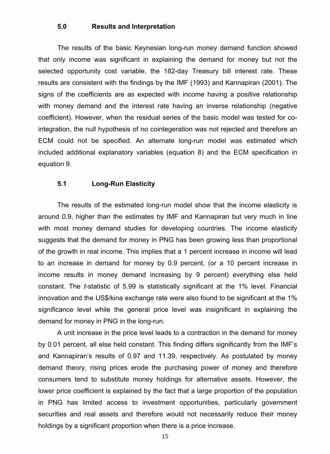
5.1 Long-Run Elasticity
The results of the estimated long-run model show that the income elasticity is
around 0.9, higher than the estimates by IMF and Kannapiran but very much in line
with most money demand studies for developing countries. The income elasticity
suggests that the demand for money in PNG has been growing less than proportional
of the growth in real income. This implies that a 1 percent increase in income will lead
to an increase in demand for money by 0.9 percent, (or a 10 percent increase in
income results in money demand increasing by 9 percent) everything else held
constant. The t-statistic of 5.99 is statistically significant at the 1% level. Financial
innovation and the US$/kina exchange rate were also found to be significant at the 1%
significance level while the general price level was insignificant in explaining the
demand for money in PNG in the long-run.
A unit increase in the price level leads to a contraction in the demand for money
by 0.01 percent, all else held constant. This finding differs significantly from the IMF’s
and Kannapiran’s results of 0.97 and 11.39, respectively. As postulated by money
demand theory, rising prices erode the purchasing power of money and therefore
consumers tend to substitute money holdings for alternative assets. However, the
lower price coefficient is explained by the fact that a large proportion of the population
in PNG has limited access to investment opportunities, particularly government
securities and real assets and therefore would not necessarily reduce their money
holdings by a significant proportion when there is a price increase.
16
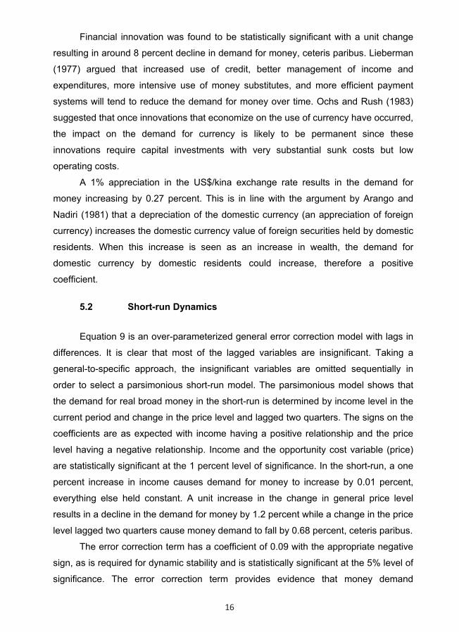
Financial innovation was found to be statistically significant with a unit change
resulting in around 8 percent decline in demand for money, ceteris paribus. Lieberman
(1977) argued that increased use of credit, better management of income and
expenditures, more intensive use of money substitutes, and more efficient payment
systems will tend to reduce the demand for money over time. Ochs and Rush (1983)
suggested that once innovations that economize on the use of currency have occurred,
the impact on the demand for currency is likely to be permanent since these
innovations require capital investments with very substantial sunk costs but low
operating costs.
A 1% appreciation in the US$/kina exchange rate results in the demand for
money increasing by 0.27 percent. This is in line with the argument by Arango and
Nadiri (1981) that a depreciation of the domestic currency (an appreciation of foreign
currency) increases the domestic currency value of foreign securities held by domestic
residents. When this increase is seen as an increase in wealth, the demand for
domestic currency by domestic residents could increase, therefore a positive
coefficient.
5.2 Short-run Dynamics
Equation 9 is an over-parameterized general error correction model with lags in
differences. It is clear that most of the lagged variables are insignificant. Taking a
general-to-specific approach, the insignificant variables are omitted sequentially in
order to select a parsimonious short-run model. The parsimonious model shows that
the demand for real broad money in the short-run is determined by income level in the
current period and change in the price level and lagged two quarters. The signs on the
coefficients are as expected with income having a positive relationship and the price
level having a negative relationship. Income and the opportunity cost variable (price)
are statistically significant at the 1 percent level of significance. In the short-run, a one
percent increase in income causes demand for money to increase by 0.01 percent,
everything else held constant. A unit increase in the change in general price level
results in a decline in the demand for money by 1.2 percent while a change in the price
level lagged two quarters cause money demand to fall by 0.68 percent, ceteris paribus.
The error correction term has a coefficient of 0.09 with the appropriate negative
sign, as is required for dynamic stability and is statistically significant at the 5% level of
significance. The error correction term provides evidence that money demand

17
adjustments occur to maintain equilibrium, and these adjustments account for a share
of the explained variation in the estimated money demand equation. The estimated
coefficient indicates that 9 percent of the disequilibrium in the previous quarter is
corrected in the current quarter and the long-run equilibrium is restored in eleven
quarters.
6.0 Conclusion
The analysis based on the variant of the basic Keynesian money demand
function shows that there is a long-run co-integrating relationship between real broad
money and the selected explanatory variables (real income, price, exchange rate and
financial innovation). Real income, financial innovation and the US$/kina exchange
rate are significant at the 1% level in the long-run. Interest rate is found to be
insignificant in the long-run. It is found that the main determinants of money demand in
PNG are income, prices (inflation in particular) and financial innovation, which is
consistent with the earlier studies. In the short-run, inflation and income are significant
at the 1% level. The significance of income and financial innovation in the long-run
imply that income and financial innovation do not necessarily change overnight but
take time and therefore in the short-run would not have a significant influence on the
demand for money but are the main determinants in the long-run.
The CUSUM and CUMSQ tests confirm that demand for money in PNG has
been stable during the period 1978Q1 to 2010Q4. The function being stable implies
that its application in monetary policy can exert a predictable influence on the real
economy. A stable money demand function hence becomes necessary for monetary
policy formulation and a useful instrument of macroeconomic policy.
Lack of appropriate and reliable time series data is a problem and hence a short
coming for this analysis. The interpolated quarterly GDP data may not be a true
reflection of the actual outcomes and therefore the results may be misleading. An
option would be to use quarterly GDP derived by Lahari et al (2009) or construct such
a series using the same techniques. In addition, the proxy for financial innovation may
not be appropriate and so alternative proxies have to be established and data on such
a proxy collected/constructed. Similarly, an appropriate market determined interest rate
should be included in the model.

18
7.0 Appendix
Table A1Descriptive Statistics
Table A2Correlation Analysis
Real M3 Real GD... CPI 182-day TBill Rate Financial Innovation USD/PGK Mean 1.756 6.051 5.782 1.104 0.113 0.809 Median 1.813 6.078 5.571 1.098 0.107 0.948 Maximum 2.517 6.442 6.970 1.253 0.186 1.553 Minimum 1.075 5.695 4.641 1.011 0.054 0.249 Std. Dev. 0.365 0.191 0.714 0.051 0.034 0.419 Skewness 0.049 0.066 0.172 0.899 0.367 0.065 Kurtosis 2.450 1.998 1.652 3.407 2.348 1.556
Jarque-Bera 1.717 5.613 10.638 18.683 5.307 11.562 Probability 0.424 0.060 0.005 0.000 0.070 0.003
Sum 231.768 798.727 763.250 145.746 14.868 106.743 Sum Sq. Dev. 17.431 4.800 66.722 0.346 0.147 23.008
Observations 132 132 132 132 132 132
Correlationt-StatisticProbability Real M3 Real GDP CPI182-day TBil...Financial in... USD/PGK
Real M3 1.000----------
Real GDP 0.884 1.00021.586 -----0.000 -----
CPI 0.717 0.833 1.00011.736 17.187 -----0.000 0.000 -----
182-day TBill rate -0.101 -0.145 -0.046 1.000-1.163 -1.676 -0.528 -----0.247 0.096 0.598 -----
Financial innova... -0.896 -0.900 -0.863 0.076 1.000-23.037 -23.546 -19.435 0.867 -----
0.000 0.000 0.000 0.387 -----
USD/PGK -0.648 -0.773 -0.960 -0.112 0.823 1.000-9.710 -13.914 -39.099 -1.280 16.549 -----0.000 0.000 0.000 0.203 0.000 -----

19
Table A3Over-parameterised ECM
Dependent Variable: D(LRM3)Method: Least SquaresDate: 11/27/14 Time: 10:41Sample (adjusted): 1979Q2 2010Q4Included observations: 127 after adjustments
Variable Coefficient Std. Error t-Statistic Prob.
C -1.047886 0.580269 -1.805861 0.0740LRY 0.187849 0.092634 2.027869 0.0453FIN 0.899742 0.614396 1.464434 0.1463
LCPI -0.018340 0.030752 -0.596384 0.5523XR -0.029782 0.045449 -0.655280 0.5138
D(LRM3(-1)) -0.251465 0.107829 -2.332064 0.0218D(LRM3(-2)) -0.078143 0.108370 -0.721072 0.4726D(LRM3(-3)) -0.070737 0.101584 -0.696343 0.4879D(LRM3(-4)) -0.084225 0.082093 -1.025972 0.3075
D(LRY) 0.171828 0.330791 0.519445 0.6046D(LRY(-1)) -0.306179 0.339106 -0.902903 0.3688D(LRY(-2)) 0.326582 0.348707 0.936553 0.3513D(LRY(-3)) -0.215109 0.340694 -0.631386 0.5293D(LRY(-4)) -0.194443 0.332134 -0.585435 0.5596
D(FIN) -2.082185 0.688885 -3.022543 0.0032D(FIN(-1)) -2.226443 0.832894 -2.673140 0.0088D(FIN(-2)) -1.974946 0.712362 -2.772391 0.0067D(FIN(-3)) -1.293464 0.633136 -2.042949 0.0438D(FIN(-4)) -0.312843 0.528278 -0.592194 0.5551D(LCPI) -1.005578 0.428063 -2.349137 0.0208
D(LCPI(-1)) -0.779925 0.453137 -1.721170 0.0884D(LCPI(-2)) -0.564445 0.443082 -1.273906 0.2057D(LCPI(-3)) -0.104029 0.430856 -0.241448 0.8097D(LCPI(-4)) -0.263828 0.435898 -0.605252 0.5464
D(XR) 0.215499 0.126951 1.697494 0.0928D(XR(-1)) 0.183124 0.125694 1.456904 0.1484D(XR(-2)) 0.013327 0.123465 0.107939 0.9143D(XR(-3)) -0.239620 0.123619 -1.938383 0.0555D(XR(-4)) 0.001814 0.123161 0.014731 0.9883
E7(-1) -0.023620 0.047400 -0.498307 0.6194
R-squared 0.474227 Mean dependent var 0.010309Adjusted R-squared 0.317037 S.D. dependent var 0.053270S.E. of regression 0.044023 Akaike info criterion -3.205242Sum squared resid 0.187989 Schwarz criterion -2.533387Log likelihood 233.5329 Hannan-Quinn criter. -2.932276F-statistic 3.016903 Durbin-Watson stat 1.980209Prob(F-statistic) 0.000027
20
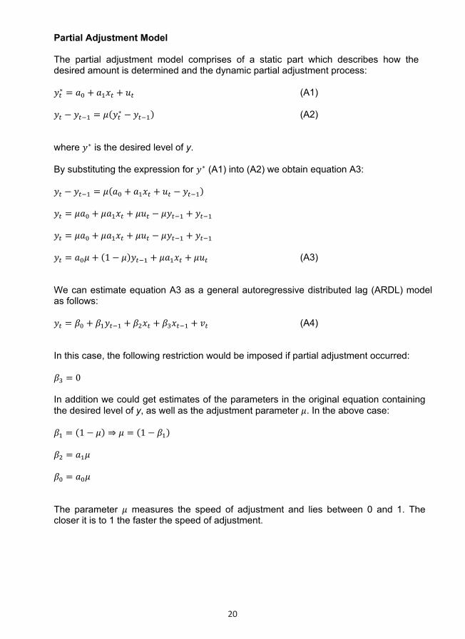
Partial Adjustment Model
The partial adjustment model comprises of a static part which describes how the desired amount is determined and the dynamic partial adjustment process:
𝑦𝑦𝑡𝑡∗ = 𝑎𝑎0 + 𝑎𝑎1𝑥𝑥𝑡𝑡 + 𝑢𝑢𝑡𝑡 (A1)
𝑦𝑦𝑡𝑡 − 𝑦𝑦𝑡𝑡−1 = 𝜇𝜇(𝑦𝑦𝑡𝑡∗ − 𝑦𝑦𝑡𝑡−1) (A2)
where 𝑦𝑦∗ is the desired level of y.
By substituting the expression for 𝑦𝑦∗ (A1) into (A2) we obtain equation A3:
𝑦𝑦𝑡𝑡 − 𝑦𝑦𝑡𝑡−1 = 𝜇𝜇(𝑎𝑎0 + 𝑎𝑎1𝑥𝑥𝑡𝑡 + 𝑢𝑢𝑡𝑡 − 𝑦𝑦𝑡𝑡−1)
𝑦𝑦𝑡𝑡 = 𝜇𝜇𝑎𝑎0 + 𝜇𝜇𝑎𝑎1𝑥𝑥𝑡𝑡 + 𝜇𝜇𝑢𝑢𝑡𝑡 − 𝜇𝜇𝑦𝑦𝑡𝑡−1 + 𝑦𝑦𝑡𝑡−1
𝑦𝑦𝑡𝑡 = 𝜇𝜇𝑎𝑎0 + 𝜇𝜇𝑎𝑎1𝑥𝑥𝑡𝑡 + 𝜇𝜇𝑢𝑢𝑡𝑡 − 𝜇𝜇𝑦𝑦𝑡𝑡−1 + 𝑦𝑦𝑡𝑡−1
𝑦𝑦𝑡𝑡 = 𝑎𝑎0𝜇𝜇 + (1 − 𝜇𝜇)𝑦𝑦𝑡𝑡−1 + 𝜇𝜇𝑎𝑎1𝑥𝑥𝑡𝑡 + 𝜇𝜇𝑢𝑢𝑡𝑡 (A3)
We can estimate equation A3 as a general autoregressive distributed lag (ARDL) model as follows:
𝑦𝑦𝑡𝑡 = 𝛽𝛽0 + 𝛽𝛽1𝑦𝑦𝑡𝑡−1 + 𝛽𝛽2𝑥𝑥𝑡𝑡 + 𝛽𝛽3𝑥𝑥𝑡𝑡−1 + 𝑣𝑣𝑡𝑡 (A4)
In this case, the following restriction would be imposed if partial adjustment occurred:
𝛽𝛽3 = 0
In addition we could get estimates of the parameters in the original equation containing the desired level of y, as well as the adjustment parameter 𝜇𝜇. In the above case:
𝛽𝛽1 = (1 − 𝜇𝜇) ⇒ 𝜇𝜇 = (1 − 𝛽𝛽1)
𝛽𝛽2 = 𝑎𝑎1𝜇𝜇
𝛽𝛽0 = 𝑎𝑎0𝜇𝜇
The parameter 𝜇𝜇 measures the speed of adjustment and lies between 0 and 1. The closer it is to 1 the faster the speed of adjustment.
21
Figure A1: Variables in Levels
Figure A2: Variables in First Difference
5.6
6.0
6.4
6.8
7.2
1980 1985 1990 1995 2000 2005 2010
Real broad money
6.8
7.0
7.2
7.4
7.6
7.8
8.0
8.2
1980 1985 1990 1995 2000 2005 2010
Real GDP
-5
0
5
10
15
20
25
1980 1985 1990 1995 2000 2005 2010
182 day Treasury bill interest rate (%)
4.5
5.0
5.5
6.0
6.5
7.0
1980 1985 1990 1995 2000 2005 2010
CPI
0.0
0.4
0.8
1.2
1.6
1980 1985 1990 1995 2000 2005 2010
US/Kina exchange rate
-3.2
-2.8
-2.4
-2.0
-1.6
1980 1985 1990 1995 2000 2005 2010
Financial innovation
-.3
-.2
-.1
.0
.1
.2
.3
1980 1985 1990 1995 2000 2005 2010
Real broad money
-.06
-.04
-.02
.00
.02
.04
.06
.08
1980 1985 1990 1995 2000 2005 2010
Real GDP
-8
-4
0
4
8
12
1980 1985 1990 1995 2000 2005 2010
182 day Treasury bill interest rate (%)
-.04
.00
.04
.08
.12
1980 1985 1990 1995 2000 2005 2010
CPI
-.16
-.12
-.08
-.04
.00
.04
.08
.12
1980 1985 1990 1995 2000 2005 2010
US/Kina exchange rate
-.3
-.2
-.1
.0
.1
.2
.3
.4
1980 1985 1990 1995 2000 2005 2010
Financial innovation

22
The ADF test procedure is as follows:
Hypothesis:
Null hypothesis: 𝐻𝐻0:𝜌𝜌 = 0 → unit root (non-stationary)
Alternative hypothesis: 𝐻𝐻1:𝜌𝜌 ≠ 0 → no unit root (stationary)
Decision:
Do not reject 𝐻𝐻0 if the calculated ADF test statistic > the critical value for the desired level
of significance (normally at 1% or 5%).
Conclusion: Variable is non-stationary.

23
References
AlBazai, S. H. 1998, “The Demand for Money in Saudi Arabia: Assessing the Role of Financial Innovation, Journal of Economic & Administrative Sciences, Vol. 14, pp.79-106
Asteriou, D and Hall, G. S. 2007, Applied Econometrics, A Modern Approach using EViews and Microfit, Revised Edition, Palgrave Macmillan
Azali, M et al. 2000, Exchange Rate and the Demand for Money in Malaysia, Universiti Putra Malaysia Press, Kualuar Lumpur
Griffiths, W.E, Hill, R.C and Lim, G.C. 2008, Principles of Econometrics 3rd Edition, John Wiley & Sons, Inc. New Jersey, USA
Ho, W.S. 2003, Money Demand in Macao and its Estimation, Monetary Authority ofMacao, Macao
Hye, Q. M. 2009, Financial Innovation and Money Demand in Pakistan, Applied Economic Research Centre, Karachi
Judd, P. J and Scadding, L. J. 1982 The Money Demand Function, Journal of Economic Literature, Vol. XX
Kannapiran, A. C. 2001, Stability of Money Demand and Monetary Policy in Papua New Guinea (PNG), International Economic Journal, Vol. 15, No. 3
Katafono, R. 2001, A Re-examination of the Demand for Money in Fiji, Working Paper 2001/03, Reserve Bank of Fiji.
Kanari, M. 1998, (unpublished), Money Demand in Papua New Guinea, Bank of PNG, Port Moresby
Lieberman, C. 1977, “The Transaction Demand for Money and Technological Change”, Review of Economics and Statistics, Vol. 59 pp. 307-317
Mundell, A. R, 1963, “Capital Mobility and Stabilisation Policy”, Canadian Journal of Economics and Political Science, 29
Ocsh, J. and Rush, M. 1983, “The Persistence of Interest Rate Effects on Demand for Currency”, Journal of Money, Credit and Banking, Vol. 15, pp.462-472
Pindyck, S. R and Rubinfeld, L. D. 1998, Econometric Models and EconometricForecasts, McGraw-Hill International Editions, Singapore
Ramanathan, R. 1989, Introductory Econometrics with Applications, Harcourt Brace Jovanovich Inc, Orlando, USA
Rao, B. B and Singh, R. 2003, Demand for Money in India: 1953-2002, University of South Pacific, Fiji

24
Romer, D. 2000, Keynesian Macroeconomics without the LM Curve, Journal of Economic Perspectives, Vol.14 Number 2
Sririam, S. 1999, Survey of Literature on Demand for Money: Theoretical and Empirical Work with Special Reference to Error Correction Models, IMF Working Paper, WP99/64
_______. 2001, A Survey of Recent Empirical Money Demand Studies, IMF Staff papers, Vol. 47, No. 3
Takaendesa, P. 2006, The Behavior and Fundamental Determinants of the Real Exchange Rate in South Africa, Rhodes University, Grahamstown, South Africa
Tillers, I. 2004, Money Demand in Latvia, Bank of Latvia
Tseng, W and Corker, R. 1991, Financial Liberalization, Money Demand and Monetary Policy in Asian Countries, Occasional Papers, IMF
Verbeek, M. 2008, A Guide to Modern Econometrics 3rd Edition, John Wiley & Sons Ltd, West Sussex, England