Embed Size (px)
Citation preview
Demand Curves and Consumer Rationing Rules
Christopher S. Ruebeck 1
Lafayette College
Department of Economics
Easton PA 18042
Prepared for the
Western Economic Association International 85th Annual Conference
June 3, 2010
First version: February 25, 2010
Preliminary, please do not cite without permission.
1 This work was funded in part through NSF grants HSD BCS-079458 and CPATH-T 0722211/0722203. I thank David Stifel, Ed Gamber, and Robert Masson for helpful comments.

Abstract
The demand curve’s shape is consequential in microeconomic theory. In determining the
outcome of oligopoly games, we move on to the residual demand curve derived from the demand
curve and participants’ behaviors. Two literature strands in oligopoly theory focus on the
residual demand curve and derived reaction functions, one strand on firms’ beliefs and the other
on rationing of demand when firms offer identical products. This investigation focuses on the
latter through agent-based modeling of consumers’ search for products to buy.
By encoding behavioral rules for such cases, we can explore the robustness of the results
from analytically solvable models that constrain rationing rules to a smaller abstracted space of
aggregated behaviors. This paper thus formalizes stated heuristics according to their behavioral
description rather than the established assumption of their average behavior, extending the
literature that has grown out of the two-stage capacity games of Kreps & Sheinkman (1983) and
Davidson and Deneckere (1986).
Ruebeck, Rationing Rules page 1
Introduction
The residual demand curve, also called the contingent demand curve, refers to the demand facing
a firm given assumptions about consumers and other firms’ behaviors. Oligopolists’ choices
depend on at least two types of beliefs. This paper does not discuss the firms’ beliefs about each
other’s actions. It investigates our more basic assumptions about which customers arrive at each
firm given the firms’ prices and capacities for production. This is also called the “rationing
rule”, the allocation of customers between firms. The literature shows that these assumptions are
consequential to the oligopoly outcome, and we will see that previous characterizations of
aggregate consumer behavior have also had unrecognized ramifications.
The literature begins with Bertrand’s (1883) critique of the Cournot (1838) equilibrium in
quantities, and the well-known assertion that “two are enough” for firms to reach the efficient
market outcome: if the firm’s strategic variable is price rather than quantity, then two firms will
undercut each other until price is marginal cost or very close to it. Reinforcing the Cournot
equilibrium as abstracting from a “capacity” decision rather than simply “quantity”, Kreps and
Scheinkman (1983) showed that a two-stage game can support price competition and a capacity
choice that is the same as the quantities chosen in Cournot’s one-stage game.
My simulations enter this discussion with Davidson and Deneckere’s (1986) demonstration
that Kreps and Scheinkman’s assumed rationing rule was consequential. Davidson and
Deneckere’s analytic and simulation results cover rationing rules in general, and in particular
Beckmann’s (1965) implementation of Shubik’s (1955) alternative to the efficient rationing rule.
Davidson and Deneckere show that only the efficient rationing rule can provide the Kreps and
Scheinkman Cournot-equivalent outcome in a two-stage game in capacities and prices. They
Ruebeck, Rationing Rules page 2

argue in addition that firms will not choose the efficient rationing rule if the two-stage game is
extended to three stages that include first choosing the rationing rule.
That original theory was developed for homogeneous goods. It has recently been expanded
to include asymmetric costs (Lepore, 2009) and differentiated goods (Boccard and Wauthy,
2010), but the efforts reported here are not about differentiation or variation in costs. Instead, I
model costless consumer search for the first product combined with search that is costly enough
in finding the second product that consumers do not continue looking past the first firm they find
with a low enough price and sufficient remaining capacity.
Rationing rules
With two firms producing homogeneous goods in a simultaneous stage game, and we study firm
2’s best response to firm 1’s decision of price and capacity. Both firms may be capacity
constrained, but our initial discussion focuses on firm 1’s constraint when considering firm 2’s
unconstrained price choice. When firm 1 cannot satisfy the entire market at its price p1, then
firm 2 is able to reach some customers with a higher price, p2 > p1. We now need a rationing rule
to specify (perhaps stochastically) which customers buy from each firm.
The efficient rationing rule is attractive for several reasons, and its shape is familiar from
exercises ‘shifting the demand curve’ that begin in Principles of Economics. Although the
implicit assumption that this rationing rule makes about allocating higher-paying customers to
the capacity-constrained firm has been known at least since Shubik’s (1955, 1959) early
discussion of game theory and market structure, there is little discussion of the consequences
outside the literature mentioned above. Figure 1 depicts this rationing rule and its implications.
Ruebeck, Rationing Rules page 3

The demand curve D(p) shifts left by the lower-priced firm’s capacity k1, as depicted by figure’s
the darker dashed lines. Formally, for p2 > p1, residual demand is given by
quantity
pric
e
Figure 1: The efficient rationing rule. Bold dashed lines represent the conventional intuition for contingent demand facing firm 2 when firm 1 chooses capacity k1 and prices at p1 in a homogeneous good market. The lightly dashed lines emphasize this rationing rule’s effect on residual demand facing firm 2.
D(p1)
p1
k1
k1
MB(k1)
D(p)
D(p2|p1)
It may not be immediately apparent how this ‘parallel shift’ of the demand curve determines
the rationing of customers between the two firms. The figure’s lightly dashed lines show that
that those units of the good with highest marginal benefit are not available to the higher-priced
firm. As we get more specific about the rationing mechanism, it is relevant to assume that this
market demand curve depicts a continuum of unitary-demand customers along the price axis.
This is rationing rule is the economically efficient outcome, hence its name. The justification
for presuming economic efficiency, though, is made on long-run grounds. So, too, is the
Ruebeck, Rationing Rules page 4
literature’s abstraction of firm interaction to a one-shot game, but both of those assumptions
jump across the divide between firms’ long-run choices, short-run choices and outcomes, and the
long-run consequences of those choices. We will return to this discussion after discussing an
alternative rationing rule used by the literature following Davidson and Denechere.
There are three portions of the firm 2’s residual demand curve D(p2|p1) depending on whether
its price p2 is less than, equal to, or greater than firm 1’s price p1. The alternative proportional
residual dmeand curve depicted in Figure 2 matches D(p) for p2 < p1 just as the efficient demand
curve in Figure 1: they both take Bertrand’s assumption that all customers buy from the lower-
priced firm if they can. In the case of a “tie”, p2 = p1, the literature makes two possible
assumptions on the discontinuity. Davidson and Deneckere assume a discontinuity on both the
right and the left of (a.k.a. above and below) p1 with the two firms splitting demand evenly up to
their production capacities. Allen and Hellwig (1993) assume a discontinuity only to the left
(below) p1, pricing at equality by extending the upper part of the curve. It may be more accurate
to characterize the upper part of the proportional curve as an extension of the outcome when
prices are equal, a point I will return to below.
Although the efficient rationing rule would appear to be an attractive characterization of a
residual demand curve “in the long run”, firms are typically making decisions and conjectures
about each other’s prices in the short run. The long run occurs as a result of firms’ shorter-term
decisions, their long-run constraints, their anticipations of each other’s decisions, and the
evolution of the market, with both consumers’ and firms’ reactions to the shorter-term decisions
affecting the long run decisions and outcome. Game theoretic characterizations of strategic
behavior in the short run are important in determining the long run, as the market’s players not
Ruebeck, Rationing Rules page 5

only react to each other but also anticipate each other’s actions. Yet, in assuming the efficient
rationing rule, the level of abstraction may penetrate further in some dimensions of the problem
than others, leading to an unattractive mismatch between the short run one-shot game and long
run outcomes. After defining the residual demand curve associated with proportional rationing,
the discussion and simulations below will show that even the short run abstraction may be
mismatched with the descriptive reasoning behind the rationing rule.
pric
e
Figure 2: The Beckamnn rationing rule. The outcome at p1 = p2 is the same as the efficient rationing rule, which lies in the interval [D(p1), D(p1) – k1]. The point (D(p1) – k1, p1) is typically not on the residual command curve, serving as the open end of the line connected to maximum demand.
D(p1)
p1
k1
D(p)
D(p2|p1)
quantity
The key feature of the proportional rationing rule, depicted in Figure 2, is that all buyers with
sufficient willingness to pay are represented in the customers that arrive at both firms. That is,
all consumers with willingness to pay at or above p2 > p1 may buy from firm 2. Thus the market
demand curve is “rotated” around its vertical intercept (the price equal to the most any customer
Ruebeck, Rationing Rules page 6

will pay) rather than “shifting” in parallel. Describing the realization of this contingent demand
curve between p1 and the maximum willingness to pay is not so intuitive as for the efficient
contingent demand curve, although the highest point is easy: the maximum of of D(p) must also
be the maximum of D(p2|p1) because both firms have a chance at every customer.
To justify the D(p2|p1) contingent demand curve at prices p2 > p1, Shubik, Beckmann,
Levitan, Davidson and Deneckere (those we may call the progenitors of this rationing rule’s use
in oligopoly theory), describe some specifics on consumers’ arrival processes and connect these
two points with a straight line, so that “the residual demand at any price is proportional to the
overall market demand at that price” (Allen and Hellwig, 1993), or as Beckmann first states it,
When selling prices of both duopolists are equal, total demand is a linear function of price. When prices of the two sellers differ, buyers will try as far as possible to buy from the low-price seller. Those who fail to do so will be considered a random sample of all demanders willing to buy at the lower price.
The actual proportion used draws directly from the efficient rationing rule. It is the fraction
of demand remaining for firm 2 if firm 1 receives demand for its entire capacity (up to firm 2’s
capacity and only greater than zero if market demand is greater than firm 1’s capacity).
Formally, the proportional contingent demand for firm 2 when at p2 > p1 is
The key feature of this rationing rule is the constant fraction (D(p1) – k1) / D(p1) that weights
the portion of market demand firm 2 receives at price p2. First, this fraction is the demand firm 2
receives when prices are equal, and second this fraction remains constant as firm 2 increases
price. The shape of the residual demand curve below will show that neither of these features
need be true as we consider consumers’ arrival at the firms.
Ruebeck, Rationing Rules page 7
Implementing random arrival
We now turn to implementing customer arrival and search rules. For the efficient rationing rule,
consumers must be sorted according to the discussion of Figure 1; they do not arrive in random
order: all customers with WTP greater than MB(k1) are sent to the capacity constrained, lower-
price firm. Somehow these customers rather than others get the good, perhaps by resale (Perry,
1984), but it is not the point of this investigation to model that process. Here we have consumers
that arrive in random order. Yet that is just one of the assumptions of the proportional rationing
rule; the other assumption is that the customers that arrive first are always allocated to the lower-
priced firm. Relaxing this second assumption is what drives the new results below.
Random arrival, random first firm
The results to follow are driven by the manner in which consumers have equal likelihood of
arriving at each firm, at any price p2. The simulation specifies that buyers arrive in random order
at two capacity-constrained sellers. The buyer chooses randomly between them; if the first
seller’s price is too high, the buyer moves on to the other one, or doesn’t buy at all if both prices
are too high. As later buyers arrive (in random order), they only consider sellers who have net
yet reached their capacity constraint.
In this discussion, as in the analytic models described above, we take the perspective of the
contingent demand facing firm 2 given firm 1’s chosen price and capacity. Note that the number
labels do not mean that buyers in the simulation arrive first at either location; they have equal
chance of arriving first at either firm 1 or firm 2.
Ruebeck, Rationing Rules page 8

Figure 3 presents an example of the simulation results. Each of the lines in the plot (some
overlapping each other) shows a statistic of 1300 runs. The plots are overlaid for six 1300-run
sets. These statistics capture the stochastic residual demand curve facing firm 2 with no capacity
constraint while the other firm sets price p1 = 9 and capacity k1 = 7. The market demand curve is
q = 24 – p. Each of the 23 buyers has unitary demand at price D23 = 23, D22 = 22, … , D1 = 1.
The proportional rationing rule is shown as constant-slope black line segments connecting the
outcomes for p = 0, 8, 9, and 24. The proportional black line segment connecting p = 8 and 9
reflects the discrete nature of demand in this simulation.
The green lines in Figure 3 are maxima and minima for firm 2’s contingent demand at each
price for each of the six 1300-run sets. There are multiple maximum and/or multiple minimum
lines at some prices p2 because they can have slightly different realizations across the six sets;
1300 simulated runs are not always enough to establish the maxima and minima for all customer
arrival outcomes. The insight from these maxima and minima statistics is that there is more
variation (the distribution’s tail is thinner) in the minima for higher prices p2, and more variation
in the maxima for lower prices p2. The theoretical maximum at each price p2 is the entire
demand curve: by chance all the customers may arrive first at Firm 2. The difficulty of reaching
that maximum in a 1300-run sample at lower p2 prices reflects the smaller chance that this tail
event can happen when there are more potential customers. The minimum at any price is 7 units
to the left of that maximum (or 0,which ever is larger), reflecting the capacity constraint of firm
1; the minimum for firm 2 is less likely to occur when 2’s price p2 is high because having all
high-value buyers arrive first at firm 2 is less likely when there are few possible buyers.
Ruebeck, Rationing Rules page 9
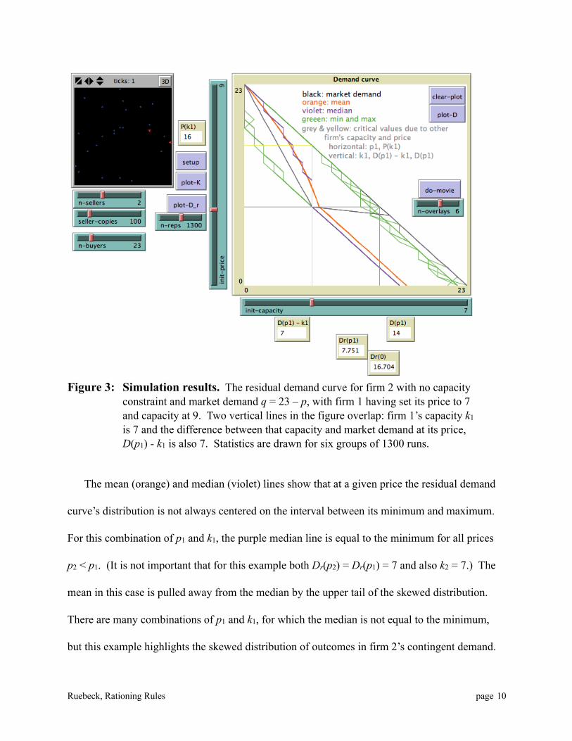
Figure 3: Simulation results. The residual demand curve for firm 2 with no capacity constraint and market demand q = 23 – p, with firm 1 having set its price to 7 and capacity at 9. Two vertical lines in the figure overlap: firm 1’s capacity k1 is 7 and the difference between that capacity and market demand at its price, D(p1) - k1 is also 7. Statistics are drawn for six groups of 1300 runs.
The mean (orange) and median (violet) lines show that at a given price the residual demand
curve’s distribution is not always centered on the interval between its minimum and maximum.
For this combination of p1 and k1, the purple median line is equal to the minimum for all prices
p2 < p1. (It is not important that for this example both Dr(p2) = Dr(p1) = 7 and also k2 = 7.) The
mean in this case is pulled away from the median by the upper tail of the skewed distribution.
There are many combinations of p1 and k1, for which the median is not equal to the minimum,
but this example highlights the skewed distribution of outcomes in firm 2’s contingent demand.
Ruebeck, Rationing Rules page 10

Figure 4 illustrates the distributions for two of firm 2‘s prices (p2 = 6 and 10) for further
confirmation of contingent demand’s skewness.
Figure 4: Simulation distributions. Two examples of the distribution of outcomes when firm 1 has set p1 = 7 and k1 = 9, as in Figure 2.
The mean residual demand curve does not change linearly with price for p2 > p1; the two
firms share the market with varying proportions rather than the usual constant proportion. We
now turn to a general discussion of this demand curve facing firm 1 given its assumptions about
firm 2.
The three sections of the plots in Figure 3 above are all substantively different from the
proportional rationing rule’s residual demand. As we have already noted and will investigate
further below, the average residual demand is larger than the proportional contingent demand
curve for p2 > p1. In addition, demand is smaller than the the usual homogeneous goods
assumption when p2 < p1: the lower-priced firm does not capture the entire market. Finally, at
equal prices p2 = p1 there is an equal chance of arrival rather than the equal sharing oe constant
proportions assumptions in the literature. The outcome at equal prices, consistent with those for
p2 above p1 is only due to the firm(s) capacity limit(s).
Ruebeck, Rationing Rules page 11
In the region where p2 > p1, the traditional proportional residual demand curve provides firm
2 with a “better” result than that provided by the efficient residual demand curve—a larger
residual demand to the higher-priced firm. The results in Figure 3 are better still for the higher-
priced firm, and firm 2’s proportion of the market grows as p2 increases rather than remaining
constant. This occurs because firm 1’s capacity constraint improves the chance that more of the
higher-value customers happen to arrive first at firm 1 instead of firm 2.
Using this customer search specification will affect firms’ equilibria in prices and capacities.
In addition to the behavioral differences and the increased market power of the higher-priced
firm (when the lower-priced firm is capacity constrained), the continuity at p2 = p1 may affect the
equilibria, in particular the existence of pure-strategy equilibria.
Allen and Hellwig (1993) state that consumers go to the first firm on a “first-come first-
served basis” and follow that with the assertion, “Firm j with the higher price pj meets the
residual demand of those consumers—if any—who were unable to buy at the lower price.”
Focusing directly on a first-come first-served rule requires that some late-arriving consumers
with pi < WTP < pj may not be served by the lower-priced firm and won’t want to buy from the
higher-priced firm.
The algorithm here (Figure 5) recognizes that the searching consumers may know very little
about the available prices available at these firms before they arrive at the firms, not the usual
assumption in search models. There is a small literature that considers this type of search, in
particular Rothschild (1973), but rather strong assumptions are still required to arrive at a model
amenable to analytic methods. Telser’s (1973) investigation finishes with the conclusion that
(emphasis added), “If the searcher is ignorant of the distribution, then acceptance of the first
Ruebeck, Rationing Rules page 12
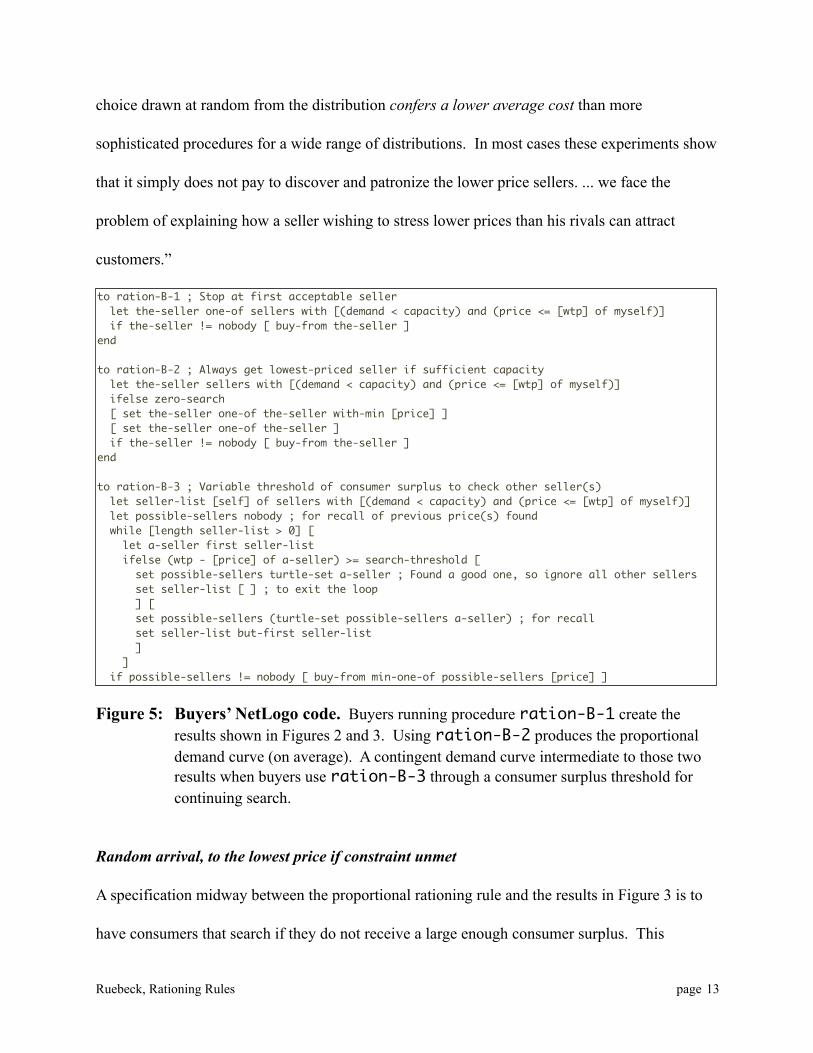
choice drawn at random from the distribution confers a lower average cost than more
sophisticated procedures for a wide range of distributions. In most cases these experiments show
that it simply does not pay to discover and patronize the lower price sellers. ... we face the
problem of explaining how a seller wishing to stress lower prices than his rivals can attract
customers.”
Figure 5: Buyers’ NetLogo code. Buyers running procedure ration-B-1 create the results shown in Figures 2 and 3. Using ration-B-2 produces the proportional demand curve (on average). A contingent demand curve intermediate to those two results when buyers use ration-B-3 through a consumer surplus threshold for continuing search.
to ration-B-1 ; Stop at first acceptable seller let the-seller one-of sellers with [(demand < capacity) and (price <= [wtp] of myself)] if the-seller != nobody [ buy-from the-seller ]end
to ration-B-2 ; Always get lowest-priced seller if sufficient capacity let the-seller sellers with [(demand < capacity) and (price <= [wtp] of myself)] ifelse zero-search [ set the-seller one-of the-seller with-min [price] ] [ set the-seller one-of the-seller ] if the-seller != nobody [ buy-from the-seller ]end
to ration-B-3 ; Variable threshold of consumer surplus to check other seller(s) let seller-list [self] of sellers with [(demand < capacity) and (price <= [wtp] of myself)] let possible-sellers nobody ; for recall of previous price(s) found while [length seller-list > 0] [ let a-seller first seller-list ifelse (wtp - [price] of a-seller) >= search-threshold [ set possible-sellers turtle-set a-seller ; Found a good one, so ignore all other sellers set seller-list [ ] ; to exit the loop ] [ set possible-sellers (turtle-set possible-sellers a-seller) ; for recall set seller-list but-first seller-list ] ] if possible-sellers != nobody [ buy-from min-one-of possible-sellers [price] ]
Random arrival, to the lowest price if constraint unmet
A specification midway between the proportional rationing rule and the results in Figure 3 is to
have consumers that search if they do not receive a large enough consumer surplus. This
Ruebeck, Rationing Rules page 13

specification could be viewed as redundant because we have already specified (i) that consumers
have a willingness-to-pay and (ii) they do not know or have any priors on the firms’ prices. It
may make more sense to specify those priors or updating of priors in future work.
We now have consumers with a willingness-to-pay and no prior beliefs about the price
distribution, just as in the previous specification, but in addition they will search further if their
consumer surplus is not high enough. In addition, they have perfect recall and can travel back to
the first . The ability to travel back to the first seller may be modified in future work to
recognize that these buyers who check a second firm’s price even though the first firm’s was
below their WTP are those with a lower consumer surplus to begin with.
Threshold changes from 0.1 to 0.2 Threshold changes from 0.2 to 0.3 Threshold changes from 0.4 to 0.5
Figure 6: Consumers who may search again. Results when the buyers use code ration-B-3 from Figure 5. Note that the regions of the residual demand curve move closer to the literature’s proportional demand demand curve as consumers become more interested in searching. The threshold is the consumer surplus as a fraction of WTP. When the threshold is 0.1, consumers try the other seller if consumer surplus is less than 10% of willingness-to-pay.
Figure 6 illustrates that this modification causes the residual demand curve to vary smoothly
from that illustrated in Figure 3 to the proportional demand curve, both for firm 2’s price above
and below the lower-priced, capacity-constrained firm 1. When p2 > p1, the choice of some
consumers to continue searching pulls the demand curve back towards the proportional
Ruebeck, Rationing Rules page 14
prediction. When p2 < p1, the choice to continue searching pushes the demand curve out towards
the usual homogeneous goods assumption. At p2 = p1, we have a discontinuity for any search
threshold that is not zero.
Further work
There are several directions in which to continue. One is to characterize this result without
simulation, by analyzing the combinatorics of the arrival process. Another is to investigate the
search rule used here. Another is to investigate the effect of this demand curve on equilibrium
outcomes, thus moving from a one-shot static analysis to a dynamic one. In equilibrium, pricing
pressure depends on the strength of the price effect compared to the output effect. Davidson and
Deneckere show that any contingent demand curve different from the efficient demand curve
must provide more market power (a larger quantity effect) to the higher-priced firm when the
other firm is capacity-constrained. Thus firms in the first stage have greater incentive to avoid
being capacity-constrained and choose capacities greater than the Cournot quantity. This leads to
an equilibrium price support in the second-stage game providing lower profits than the Cournot
outcome.
The results of this investigation show that this pressure is even stronger when we take
seriously the assumptions underlying the proportional contingent demand curve: setting a price
above one’s competitor leads to less loss of demand, market power remains for the higher-priced
firm is even larger than in the proportional case. Yet being consistent with those assumptions
also causes undercutting to be less profitable: the lower-priced unconstrained firm does not
receive all demand as assumed generally in the literature on homogeneous products. Thus
Ruebeck, Rationing Rules page 15

without further analysis we are left only with an indeterminate effect on equilibrium outcomes:
they may be either more or less competitive than than the Davidson and Deneckere result.
References
Allen, B. and Hellwig, M. 1993. “Bertrand-Edgeworth duopoly with proportional residual demand” International Economic Review 34(1):39-60.
Boccard, N. and Wauth, X. 2010. “Equilibrium vertical differentiation in a Bertrand model with capacity precommitment” International Journal of Industrial Organization forthcoming.
Beckmann, M. 1965. “Edgeworth-Bertrand duopoly revistied” in R. Henn, ed., Operations Research Verfahren III, Meisenhein: Verlag Anton Hain.
Bertrand, J. 1883. “Théorie mathématique de la richesse sociale (review)”, Journal des Savants, Paris: September.
Cournot, A. 1883. Researches into the Mathematical Principles of Wealth, London: Macmillan.
Davidson, C. and Deneckere, R. 1986. “Long-run competition in capaity, short-run competition in price, and the Cournot model” The RAND Journal of Economics, 17(3): 404-415.
Edgeworth, F. 1925. “The Pure Theory of Monopoly” in Edgeworth, Papers Relating to Political Economy, Vol. I, New York: Burt Franklin, ch. E.
Kreps, D. and Scheinkman, J. 1983. “Precommitment and Bertrand competition yield Cournot outcomes” The Bell Journal of Economics, 14(2): 326-337.
Lepore, J. 2009. “Consumer rationing and the Cournot outcome” B.E. Journal of Theoretical Economics 9(1, Topics ): Article 28.
Levitan, R. and Shubik, M. 1972. “Price duopoly and capacity constraints” International Economic Review, 13(1): 111-122.
Perry, M. 1984. "Sustainable Positive Profit Multiple-Price Strategies in Contestable Markets" Journal of Economic Theory, 32(2): 246-265.
Ruebeck, Rationing Rules page 16

Rothschild, M. 1974. “Searching for the lowest price when the distribution of prices is unkknown” The Journal of Political Economy, 82(4)689-711.
Shubik, M. 1955. “A comparison of treatments of a duopoly problem” Econometrica, 23(4): 417-431.
Shubik, M. 1959. Strategy and Market Structure: Competition, Oligopoly, and the Theory of Games, New York: John Wiley & Sons.
Telser, L. 1973. “Searching for the lowest price” American Economic Review 63(2)40-49.
Ruebeck, Rationing Rules page 17