Demand Controlled Ventilation and Classroom Ventilation

William J. Fisk, Mark J. Mendell, Molly Davies, Ekaterina Eliseeva, David Faulkner, Tienzen Hong, Douglas P. Sullivan

May 2012

The research reported here was supported by the California Energy Commission Public Interest Energy Research Program, Energy-Related Environmental Research Program, award number 500-09-049.The study was additionally supported by the Assistant Secretary for Energy Efficiency and Renewable Energy, Building Technologies Program of the U.S. Department of Energy under contract DE-AC02-05CH11231.

DISCLAIMER

This document was prepared as an account of work sponsored by the United States Government. While this document is believed to contain correct information, neither the United States Government nor any agency thereof, nor The Regents of the University of California, nor any of their employees, makes any warranty, express or implied, or assumes any legal responsibility for the accuracy, completeness, or usefulness of any information, apparatus, product, or process disclosed, or represents that its use would not infringe privately owned rights. Reference herein to any specific commercial product, process, or service by its trade name, trademark, manufacturer, or otherwise, does not necessarily constitute or imply its endorsement, recommendation, or favoring by the United States Government or any agency thereof, or The Regents of the University of California. The views and opinions of authors expressed herein do not necessarily state or reflect those of the United States Government or any agency thereof, or The Regents of the University of California.

Ernest Orlando Lawrence Berkeley National Laboratory is an equal opportunity employer.

i

Acknowledgements The authors thank Brad Meister of the California Energy Commission for project management, Brad Meister, Martha Brook, Maziar Shirakh, Curt Klaassen, Xiaohui Zhou, Michael McGaraghan, Jim Meacham, and Cathy Chappell for their input in the process leading to recommended changes in Title 24 related to demand controlled ventilation, Mark Hydeman and Steve Taylor at Taylor Engineering for providing cost data for the demand controlled ventilation systems, Dennis DiBartolomeo for assistance with electronics and software, Mike Spears for collecting some of the data in the study of optical people counting systems, and the following individuals for reviewing drafts of interim documents on which this report is based: Mike Apte, Fred Buhl, Curt Klaassen, Mike Sohn.

ii

ABSTRACT This document summarizes a research effort on demand controlled ventilation and classroom ventilation. The research on demand controlled ventilation included field studies and building energy modeling. Major findings included:

• The single-location carbon dioxide sensors widely used for demand controlledventilation frequently have large errors and will fail to effectively control ventilationrates (VRs).

• Multi-location carbon dioxide measurement systems with more expensive sensorsconnected to multi-location sampling systems may measure carbon dioxide moreaccurately.

• Currently-available optical people counting systems work well much of the time buthave large counting errors in some situations.

• In meeting rooms, measurements of carbon dioxide at return-air grilles appear to be abetter choice than wall-mounted sensors.

• In California, demand controlled ventilation in general office spaces is projected to savesignificant energy and be cost effective only if typical VRs without demand controlledventilation are very high relative to VRs in codes.

Based on the research, several recommendations were developed for demand controlled ventilation specifications in the California Title 24 Building Energy Efficiency Standards.

The research on classroom ventilation collected data over two years on California elementary school classrooms to investigate associations between VRs and student illness absence (IA). Major findings included:

• Median classroom VRs in all studied climate zones were below the California guideline,and 40% lower in portable than permanent buildings.

• Overall, one additional L/s per person of VR was associated with 1.6% less IA.

• Increasing average VRs in California K-12 classrooms from the current average to therequired level is estimated to decrease IA by 3.4%, increasing State attendance-basedfunding to school districts by $33M, with $6.2 M in increased energy costs. Further VRincreases would provide additional benefits.

• Confirming these findings in intervention studies is recommended.

• Energy costs of heating/cooling unoccupied classrooms statewide are modest, but alarge portion occurs in relatively few classrooms.

Keywords: absence, buildings, carbon dioxide, demand-controlled ventilation, energy, indoor air quality, schools, ventilation

iii

TABLE OF CONTENTS

ACKNOWLEGEMENT............................................................................................................................ii

ABSTRACT ..............................................................................................................................................iii

TABLE OF CONTENTS ..........................................................................................................................iv

List of Figures ........................................................................................................................................viii

LIST of Tables ..........................................................................................................................................ix

EXECUTIVE SUMMARY ........................................................................................................................ 1

Introduction ............................................................................................................................................ 1

Purpose .................................................................................................................................................... 1

Demand Controlled Ventilation .......................................................................................................... 2

Classroom Ventilation ........................................................................................................................... 7

CHAPTER 1: ............................................................................................................................................... 9

Introduction ............................................................................................................................................... 9

CHAPTER 2: Accuracy of CO2 Sensors Used for Demand Controlled Ventilation ................... 11

2.1. Background ............................................................................................................................... 11

2.2. Methods ..................................................................................................................................... 13

2.2.1. Field studies of single-location CO2 sensor performance ........................................... 13

2.2.2. Evaluation of faulty single-location CO2 sensors ........................................................ 17

2.2.3. Pilot evaluation of CO2 demand controlled ventilation with multi-location sampling systems ............................................................................................................................. 18

2.2.4. Pilot evaluation of spatial variability of CO2 concentrations in meeting rooms ..... 20

2.3. Results ........................................................................................................................................ 21

2.3.1 Field studies of single-location CO2 sensor performance ........................................... 21

2.3 .2. Evaluation of faulty single-location CO2 sensors ....................................................... 31

2.3.3. Pilot evaluation of CO2 demand controlled ventilation with multi-location sampling systems ............................................................................................................................. 34

2.3.4. Spatial variability of CO2 concentration in meeting rooms........................................ 38

2.4 Discussion ................................................................................................................................. 41

2.4.1 Accuracy requirements ................................................................................................... 41

2.4.2 Accuracy of single-location CO2 sensors ...................................................................... 41

2.4.3 Accuracy multi-location CO2 monitoring systems ...................................................... 43

2.4.4 Spatial variability of CO2 concentration in meeting rooms........................................ 43

iv

DISCLAIMER.............................................................................................................................................i

2.4.5 Overall findings and their implications ........................................................................ 44

2.6. Conclusions ............................................................................................................................... 45

CHAPTER 3: Assessment of Energy Savings Potential from Use of Demand Controlled Ventilation in General Office Spaces in California ......................................................................... 46

3.1. Background ............................................................................................................................... 46

3.2. Methods ..................................................................................................................................... 47

3.2.1. The medium size office building ................................................................................... 48

3.2.2. Outdoor air ventilation rates .......................................................................................... 49

3.2.3. Simulation tool ................................................................................................................. 51

3.2.4. Cost estimates ................................................................................................................... 52

3.3. Results ........................................................................................................................................ 52

3.4. Discussion ................................................................................................................................. 57

3.5. Conclusions ............................................................................................................................... 58

CHAPTER 4: Optical People Counting for Demand Controlled Ventilation – A Pilot Study of Counter Performance .............................................................................................................................. 59

4.1. Background ............................................................................................................................... 59

4.2. Methods ..................................................................................................................................... 60

4.3. Results ........................................................................................................................................ 62

4.3.1. People Counting System Number 1 .............................................................................. 62

4.3.2. People Counting System Number 2 .............................................................................. 65

4.4. Discussion ................................................................................................................................. 69

4.4.1. People Counting System Number 1 .............................................................................. 69

4.4.2. People Counting System Number 2 .............................................................................. 69

4.4.3. General Observations ...................................................................................................... 70

4.5. Conclusions ............................................................................................................................... 71

CHAPTER 5: Recommended Changes to Specifications for Demand Controlled Ventilation in California’s Title 24 Building Energy Efficiency Standards ...................................................... 72

5.1. Background ............................................................................................................................... 72

5.2. Existing Specifications in Title 24 for Demand Controlled Ventilation ........................... 72

5.3. Key related research results .................................................................................................... 73

5.3.1. CO2 measurement accuracy ............................................................................................ 73

5.3.2. Spatial variability of CO2 concentrations in occupied meeting rooms ..................... 74

5.3.3. Performance of optical people counters........................................................................ 75

v

5.3.4. Energy savings potential from demand controlled ventilation in occupied meeting rooms 75

5.4. Recommendations .................................................................................................................... 75

5.4.1. Recommendation 1 .......................................................................................................... 76

5.4.2. Recommendation 2 .......................................................................................................... 77

5.4.3. Recommendation 3 .......................................................................................................... 78

5.4.4. Recommendation 4 .......................................................................................................... 78

5.4.5. Recommendation 5 .......................................................................................................... 79

5.4.6. Recommendation 6 .......................................................................................................... 80

5.4.7. Recommendation 7 .......................................................................................................... 80

5.5. Discussion ................................................................................................................................. 81

CHAPTER 6: Relationship of Classroom Ventilation Rates with Student Absence ................ 82

6.1. Background ............................................................................................................................... 82

6.2. Methods ..................................................................................................................................... 83

The associations of VRs with absence were quantified using statistical models that controlled for several potential confounding factors including socio-economic status, grade level, gender mix, and class size. (The energy costs of classroom ventilation and some financial implications to school districts and families from changes in absence rates were also estimated. These will be reported in Chapter 7.) ................................................................. 83

6.2.1. Sample design and selection for epidemiologic analysis ................................................. 83

6.2.2. Data variables for epidemiologic analysis ......................................................................... 84

6.2.3. Data management and epidemiologic analysis methods ................................................. 86

6.2.4. Estimating potential benefits of increased ventilation rates ............................................ 87

6.3. Results ............................................................................................................................................. 88

6.3.1. Modeling results ..................................................................................................................... 95

6.3.2. Estimated benefits from increased VRs ............................................................................ 101

6.4. Discussion .................................................................................................................................... 102

6.4.1. Prior findings ........................................................................................................................ 103

6.4.2. Strengths and limitations of study ..................................................................................... 105

6.4.3. Implications........................................................................................................................... 106

6.4.4. Conclusions ........................................................................................................................... 106

CHAPTER 7: Cost and Benefit Analyses Related to Different Levels of Classroom Ventilation Rates, Student Absence, and Energy Use ................................................................... 108

7.1. Background ............................................................................................................................. 108

vi

7.2. Methods ................................................................................................................................... 108

7.2.1. Comparing costs and benefits of increasing current ventilation rates in California K-12 classrooms .................................................................................................................................. 108

7.2.2. Estimating potential savings in energy and financial costs from heating and cooling classroom only when necessary ................................................................................................... 110

7.3. Results ........................................................................................................................................... 114

7.3.1. Comparing costs and benefits of increasing current ventilation rates in California K-12 classrooms .................................................................................................................................. 114

7.3.2. Estimating potential savings in energy and financial costs from heating and cooling classroom only when necessary ................................................................................................... 116

7.4. Discussion ............................................................................................................................... 118

7.4.1 Comparing costs and benefits of increasing current ventilation rates in California K-12 classrooms ....................................................................................................................................... 118

7,4.2 Estimating potential savings in energy and financial costs from heating and cooling classroom only when necessary] .................................................................................................. 119

7.5. Conclusions ............................................................................................................................. 119

REFERENCES ........................................................................................................................................ 121

GLOSSARY ............................................................................................................................................ 125

APPENDIX A: Primary data from evaluation of accuracy of CO2 sensors ................................. 127

APPENDIX B: Excerpts from specifications for demand controlled ventilation in Title 24 and its appendices ........................................................................................................................................ 133

APPENDIX C: Current ventilation standards per State of California and ASHRAE .............. 136

APPENDIX D: Calculations for comparisons to findings of Shendell et al. (2004). ................ 138

vii

LIST OF FIGURES

Figure 2.2.1: Example of measurement errors of reference CO2 instrument when measuring precise dilutions of the span gas. ................................................................ 15

Figure 2.2.2: Errors in measuring the concentration of nine CO2 calibration gases with the reference CO2 instrument. ......................................................................................... 15

Figure 2.2.3: Schematic representation of one of three systems employed to rapidly measure indoor carbon dioxide concentrations at three indoor locations per system................................................................................................................................................ 20

Figure 2.3.1: Frequency distributions of key results from the multi-concentration calibration checks. .............................................................................................................. 24

Figure 2.3.2: Errors at 760 and 1010 ppm versus manufacturer code from multi-concentration calibration checks. .................................................................................... 24

Figure 2.3.3: Errors at 760 and 1010 ppm versus sensor design type from multi-concentration calibration checks. .................................................................................... 25

Figure 2.3.4: Errors at 760 and 1010 ppm versus sensor age from multi-concentration calibration checks. The error bars represent one standard deviation in the error. . 25

Figure 2.3.5: Frequency distribution of error from single-concentration calibration checks and multi-concentration calibration challenges at 510 ppm ........................... 28

Figure 2.3.6: Error from single-concentration calibration checks and multi-concentration calibration challenges at 510 ppm plotted versus manufacturer and sensor design type. ...................................................................................................................................... 28

Figure 2.3.7: Error from single-concentration calibration checks and multi-concentration calibration challenges at 510 ppm plotted versus sensor age. The error bars represent one standard deviation in the error. .............................................................. 29

Figure 2.3.8: Improvement in accuracy of sensor FS4 after implementing the manufacturer’s recommended calibration protocol. ...................................................... 34

Figure 2.3.9: Improvement in accuracy of sensor FS7 during early period of operation in the laboratory. ................................................................................................................. 34

Figure 2.3.10: Results of evaluations of the multi-location CO2 measurement system in building M2. ......................................................................................................................... 38

Figure 1.3.11: First example of data from studies of spatial distributions of CO2 concentrations in occupied meeting rooms. .................................................................. 39

Figure 2.2.12: Second example of data from studies of spatial distributions of CO2 concentrations in occupied meeting rooms. .................................................................. 40

Figure 3.2.1: Three dimensional view the office building with typical floor plan ............. 48 Figure 3.2.2: Occupancy schedule of office building ........................................................... 49 Figure 3.3.1: Demand controlled ventilation life cycle cost savings with design

occupancy of 10.8 people / 100 m2 and base case minimum ventilation rates of 13.2 or 38.2 L/s per person. ............................................................................................. 54

Figure 3.3.2: Demand controlled ventilation life cycle cost savings with a design occupancy of 16.1 people / 100 m2 and base case minimum ventilation rates of 13.2 or 38.2 L/s per person. ............................................................................................. 54

viii

Figure 3.3.3: Demand controlled ventilation life cycle cost savings with a design occupancy of 21.5 people / 100 m2 and base case minimum ventilation rates of 13.2 or 38.2 L/s per person. ............................................................................................. 55

Figure 6.3.1: Climate regions included ................................................................................... 89 Figure 6.3.2: Estimated proportional change in illness absence with increase of 1 L/s

per person of VR within the observed range of 1-20 L/s per person, using four ventilation metrics with different averaging periods* .................................................... 98

Figure 6.3.3: Predicted relationship between ventilation rate and proportion illness absence in three California school districts .................................................................... 99

Figure 7.2.1: Example of cyclic oscillation in indoor air temperature data indicating space cooling, during two weekend days. .................................................................... 112

LIST OF TABLES

Table 2.3.1: Primary results of the multi-concentration calibration checks of 90 sensors................................................................................................................................................ 23

Table 2.3.2: Proportions of CO2 sensors in various sensor categories with errors greater than ±75 and ±100 ppm in the multi-concentration calibration checks. ....... 26

Table 2.3.3: Primary results of the single-concentration calibration checks and multi-concentration calibration challenges at 510 ppm. ......................................................... 27

Table 2.3.4: Differences in averages of absolute value errors that were statistically significant (p<0.05)* ........................................................................................................... 31

Table 2.3.5: Properties of faulty sensors evaluated in the laboratory and key findings. 33 Table 2.3.6: Results of evaluations of multi-location CO2 measurement systems in

Building M1. ........................................................................................................................ 37 Table 2.3.7: Spatial variability of CO2 concentrations in occupied meeting rooms. The

numbers are averages and standard deviations for 30 – 90 minute meetings, unless indicated otherwise. .............................................................................................. 40

Table 3.2.1: Internal loads and minimum ventilation rate of office buildings ................... 48 Table 3.2.2: Five typical California climate zones ................................................................ 49 Table 3.2.3: Minimum outdoor air requirement .................................................................... 51 Table 3.3.1: Calculated annual energy usage and net present value of costs savings . 53 Table 3.3.2: Determination of base case minimum ventilation rates above which

demand controlled ventilation become cost effective with Title 24 occupant density of 10.8 people per 100 m2 ................................................................................................. 57

Table 4.3.1: Results of controlled tests of PCS1 at a single interior door entrance to a laboratory, the numbers are averages of three repeated challenges. ....................... 63

Table 4.3.2: Results of controlled tests of PCS1 system at a four-door entrance of an office building*. ................................................................................................................... 64

Table 4.3.3: Counting accuracy of PCS1 system with naïve occupants passing through a two-door entrance to a conference room. ................................................................... 65

Table 4.3.4: Counting accuracy of PCS1 system with naïve occupants passing through a four-door door entrance to an office building. ............................................................ 65

ix

Table 4.3.6: Results of controlled tests of PCS2 at a single interior door entrance to room Room 3. The numbers are averages of three repeated challenges. ............... 67

Table 4.3.7: Counting accuracy of PCS2 with naïve occupants passing through single-door entrances to Conference Rooms 1 and 2. ............................................................ 68

Table 6.3.1: Descriptive information on selected study variables ..................................... 90 Table 6.3.2: Distribution of estimated equilibrium indoor CO2 concentrations* and

estimated ventilation rates by district, building type, and ventilation type ................. 91 Table 6.3.3: Demographic and illness absence data ........................................................... 92 Table 6.3.4: Unadjusted IRR estimates* and 95% confidence intervals (CI)** from zero

inflated negative binomial models for association between classroom ventilation rate (VR) metrics and daily classroom proportion of illness absence, per increase of 1 L/s per person VR in observed range of 1-20 L/s per person .................................. 94

Table 6.3.5: Adjusted IRR estimates* and 95% confidence intervals (CI)** from zero inflated negative binomial models for association between classroom ventilation rate (VR) metrics and daily classroom proportion of illness absence, per increase of 1 L/s per person VR in observed range of 1-20 L/s per person .................................. 97

Table 6.3.6: Predicted proportion of illness absence at specified outdoor air ventilation rates, based on adjusted models* using 7-day averaged ventilation rates, in 3 California climate zones .................................................................................................. 100

Table 6.3.7: Estimated losses in revenue to school districts (Equation 2) .................... 101 Table 7.3.1: Estimates of the energy use and costs for cooling and heating the

ventilation air provided to classrooms in California**, and potential benefits, at several ventilation rates. ................................................................................................. 115

Table 7.3.2: Summary information from analyses of periods of unnecessary heating and space cooling. ........................................................................................................... 117

Table 7.3.3: Estimates statewide energy use and energy costs from unnecessary heating and cooling of grade K-12 classrooms. .......................................................... 118

x

EXECUTIVE SUMMARY Introduction This project focuses on ventilation of buildings. Ventilation, the supply of outdoor air to a building, is necessary to control indoor air concentrations of indoor-generated air pollutants. From an energy efficiency perspective, the amount of ventilation during hot and cold weather should be minimized because ventilation air must often be heated or cooled and dehumidified. Prior research has shown that, on average, in offices and schools with higher rates of ventilation, the occupants are more satisfied with air quality, have fewer adverse health symptoms, have a slightly higher level of work performance, and have lower absence rates; however, data are sparse. Approximately nine percent of energy used in the stock of U.S. commercial buildings is attributable to heating and cooling ventilation air supplied mechanically with fans and through uncontrolled air infiltration through the building envelope. No comparable estimates are available for California’s commercial buildings, but the fraction of total building energy attributable to ventilation is likely to be comparable or moderately smaller in California.

Given the impacts of ventilation on both indoor environmental quality and energy consumption, in the selection of ventilation rates one must strike a balance between these two important concerns. Minimum ventilation standards have been established that specify minimum design ventilation rates for various types of buildings. In California, these minimum ventilation rates are specified in the California Building Energy Efficiency Standards. Due to a paucity of data, the scientific underpinning for current minimum ventilation standards is relatively weak, particularly for buildings other than offices. In addition to the need for scientifically-based minimum ventilation standards, it is important to effectively control the amount of ventilation provided to buildings.

This research project focuses on a technology for controlling ventilation rates called demand controlled ventilation. Another key element of this research project was designed to help fill the gap in knowledge related to minimum ventilation requirements in classrooms.

Purpose This research was performed to provide information than can be utilized when the California Building Energy Efficiency Standards are revised and also to help building designers and operators make better decisions pertaining to demand controlled ventilation and classroom ventilation.

1

Demand Controlled Ventilation

Carbon dioxide (CO2) sensors are often deployed in commercial buildings to obtain CO2 data that are used, in demand-controlled ventilation, to automatically modulate rates of outdoor air ventilation. Reasonably accurate CO2 measurements are needed for successful demand controlled ventilation; however, prior research has suggested substantial measurement errors. Accordingly, this study evaluated: (a) the accuracy of 208 CO2 single-location sensors located in 34 commercial buildings, b) the accuracy of four multi-location CO2 measurement systems that utilize tubing, valves, and pumps to measure at multiple locations with single CO2 sensors, and c) the spatial variability of CO2 concentrations within meeting rooms. The field studies of the accuracy of single-location CO2 sensors included multi-concentration calibration checks of 90 sensors in which sensor accuracy was checked at multiple CO2 concentrations using primary standard calibration gases. From these evaluations, average errors were small, -26 ppm and – 9 ppm at 760 and 1010 ppm, respectively; however, the averages of the absolute values of error were 118 ppm (16%) and 138 ppm (14%), at concentrations of 760 and 1010 ppm, respectively. The calibration data were generally well fit by a straight line, as indicated by high values of R2. The California Building Energy Efficiency Standards specify that sensor error must be certified as no greater than 75 ppm for a period of five years after sensor installation. At 1010 ppm, 40% of sensors had errors greater than ±75 ppm and 31% of sensors have errors greater than ±100 ppm. At 760 ppm, 47% of sensors had errors greater than ±75 ppm and 37% of sensors had errors greater than ±100 ppm. A significant fraction of sensors had errors substantially larger than 100 ppm. For example, at 1010 ppm, 19% of sensors had an error greater than 200 ppm and 13% of sensors had errors greater than 300 ppm. The field studies also included single-concentration calibration checks of 118 sensors at the concentrations encountered in the buildings, which were normally less than 500 ppm during the testing. For analyses, these data were combined with data from the calibration challenges at 510 ppm obtained during the multi-concentration calibration checks. For the resulting data set, the average error was 60 ppm and the average of the absolute value of error was 154 ppm. Statistical analyses indicated that there were statistically significant differences between the average accuracies of sensors from different manufacturers. Sensors with a “single lamp single wavelength” design tended to have a statistically significantly smaller average error than sensors with other designs except for “single lamp dual wavelength” sensors, which did not have a statistically significantly lower accuracy. Sensor age was not consistently a statistically significant predictor of error. Errors based on the CO2 concentrations displayed by building energy management systems were generally very close to the errors determined from sensor displays (when available). The average of the absolute value of the difference between 113 paired estimates of error was 25

2

ppm; however, excluding data from two sensors located within the same building, the average difference was 10 ppm. These findings indicate that the substantial measurement errors found in this study are sensor errors, not errors in translating the sensor output signals to the energy management systems. Laboratory-based evaluations of nine sensors with large measurement errors did not identify definite causes of sensor failures. The study did determine that four of the nine sensors had an output signal that was essentially invariable with CO2 concentration; i.e., the sensors were non-functional yet still deployed. The evaluations did identify slight soiling or corrosion of optical cells and, in two sensors, holes in the fabrics through which CO2 diffuses into optical cells that may possibly have contributed to performance degradations. In one of two cases when the manufacturer’s calibration protocol could be implemented, sensor accuracy was clearly improved after the protocol was implemented. The Iowa Energy Center recently released the results from a laboratory-based study of the accuracy of 15 models of new single-location CO2 sensors. Although their report does not provide summary statistics, their findings are broadly consistent with the findings of the field studies of CO2 sensor accuracy described in this report. Many of the new CO2 sensors had errors greater than 75 ppm and errors greater than 200 ppm were not unusual. In 13 buildings, the facility manager provided data on the CO2 set point concentration above which the demand controlled ventilation system increased the rate of ventilation. The reported set point concentrations ranged from 500 ppm (one instance) to 1100 ppm. The building-weighted-average set point concentration was 860 ppm. When asked, no facility manager indicated that they had calibrated sensors since sensor installation. In a pilot study of the accuracy of multi-location CO2 measurement systems, data were collected from systems installed in two buildings. The same manufacturer provided the multi-location measurement systems used in both buildings. In the first building, for the range of CO2 concentrations of key interest, the average and standard deviation in error in the indoor minus outdoor CO2 concentration difference were 14 ppm and 39 ppm, respectively, and in 16 of 18 cases the error was 36 ppm or smaller. In the second building, the measured CO2 concentrations were consistently approximately 110 ppm greater than the CO2 concentration measured with the reference CO2 instrument. Outdoor CO2 concentrations measured by the building’s measurement system averaged approximately 510 ppm which is approximately 110 ppm larger than the typical outdoor air CO2 concentration. In both of these buildings, the error in the difference between indoor and outdoor CO2 concentration, which is the appropriate control input for demand controlled ventilation, was small except at a couple measurement locations. Multi-point measurements of CO2 concentrations were completed in occupied meeting rooms to provide information for selecting sensor installation locations. Data were analyzed for 30 to 90 minute periods of meeting room occupancy. The Title 24 standard requires that CO2 be

3

measured between 0.9 and 1.8 m (3 and 6 ft) above the floor. The results of the multi-point measurements varied among the meeting rooms. In some instances, concentrations at different wall-mounted sample points varied by more than 200 ppm and concentrations at these locations sometimes fluctuated rapidly. These concentration differences may be a consequence, in part, of the high concentrations of CO2 (e.g., 50,000 ppm) in the exhaled breath of nearby occupants. In four of seven data sets, the period-average CO2 concentration at return grilles were within 5% of the period-average of all CO2 concentration measurements made at locations on walls; for the other three data sets the deviations were 7, 11, and 16%. Return-air CO2 concentrations were not consistently higher or lower than the average concentration at locations on walls. In four data sets, the period-average return-air CO2 concentration was between the lowest and highest period-average concentration measured at wall locations, while in the other three data sets the period average concentrations were lowest at the return grilles. There was no consistent increase or decrease in CO2 concentrations with height.

As an alternative to CO2 sensors, devices that use optical methods to count people as they enter and exit a building or room could provide the control signal for demand controlled ventilation. A pilot scale study evaluated the counting accuracy of two people counting systems, one a commercially-available product and the second a prototype provided by a company. The evaluations included controlled challenges of the people counting systems using pre-planned movements of occupants through doorways and evaluations of counting accuracies when naïve occupants (i.e., occupants unaware of the counting systems) passed through the entrance doors of the building or room. The two people counting systems had high counting accuracy accuracies, with errors typically less than 10%, for typical non-demanding counting events. However, counting errors were high in some highly challenging situations, such as multiple people passing simultaneously through a door. Counting errors, for at least one system, can be very high if people stand in the field of view of the sensor. Both counting system have limitations and would need to be used only at appropriate sites and where the demanding situations that led to counting errors were rare.

Demand controlled ventilation is most common used is spaces such as meeting rooms with high and variable occupancy. Another element of the research was modeling to assess the potential energy savings from use of demand controlled ventilation in general office spaces. A prototypical office building meeting the prescriptive requirements of the 2008 California building energy efficiency standards was used in EnergyPlus simulations to calculate the energy savings potential of demand controlled ventilation in five typical California climates per three design occupancy densities and two minimum ventilation rates. The assumed minimum ventilation rates in offices without demand controlled ventilation, based on two different measurement methods employed in a large survey, were 38 and 13 L/s per occupant. The results of the life cycle cost analysis show demand controlled ventilation is cost effective for office spaces if the typical minimum ventilation rate without demand controlled ventilation is 38 L/s per person, except at the low design occupancy of 10.8 people per 100 m2 in climate zones 3 (north coast) and 6 (south Coast). Demand controlled ventilation was not found to be cost effective if the typical minimum ventilation rate without demand controlled ventilation is 13 L/s per occupant, except at high design occupancy of 21.5 people per 100 m2 in climate zones 14

4

(desert) and 16 (mountains). Until the large uncertainties about the base-case ventilation rates in offices without demand controlled ventilation are reduced, the case for requiring demand controlled ventilation in general office spaces will be a weak case. With an office occupant density of 10.8 people per 100 m2, demand controlled ventilation becomes cost effective when the base-case minimum ventilation rate is greater than 42.5, 43.0, 24.0, 19.0, and 18.0 L/s per person for climate zone 3, 6, 12, 14, and 16 respectively.

Together, the findings from the laboratory studies of the Iowa Energy Center and findings from this project indicate that many CO2 based demand controlled ventilation systems will, because of poor sensor accuracy, fail to meet the design goals of saving energy while assuring that ventilation rates meet code requirements. Given this situation, one must question whether the current prescriptions for demand controlled ventilation in the California Building Energy Efficiency Standards standard are adequate. However, given the importance of ventilation and the energy savings potential of demand controlled ventilation, technology improvement activities by industry as well as further research are warranted. Some possible technical options for improving the performance of demand controlled ventilation are listed below:

• Manufacturers of single-location CO2 sensors for demand controlled ventilation applications change technologies to improve CO2 sensor accuracy. Sensor costs are likely to increase.

• Users of CO2 sensors for demand controlled ventilation applications perform sensor calibrations immediately after initial sensor installation and periodically thereafter. Research is needed to determine if such a protocol would lead to acceptable accuracy and whether costs are acceptable.

• Demand controlled ventilation systems employ existing CO2 sensors that are more accurate, stable, and expensive than the sensors traditionally used for demand controlled ventilation. To spread the cost of these sensors, multi-location sampling systems may be necessary. The pilot scale evaluations of this option included in this project are too limited for conclusions but suggest that these systems may be more accurate. System costs will need to be reduced.

• Demand controlled ventilation systems utilize sensors that count occupants, as opposed to sensors that measure CO2 concentrations.

With respect to selecting locations for CO2 sensors in meeting rooms, this research did not result in definitive guidance; however, the results suggest that measurements at return-air grilles may be preferred to measurements at wall-mounted locations.

This research led to seven recommendations for the specifications for demand controlled ventilation in the 2008 California Building Energy Efficiency Standards. These recommendations follow:

1. CO2 sensors installed in new installations of demand controlled ventilation shall have inlet ports and written protocols that make it possible to calibrate the deployed sensors using CO2 calibration gas samples. The inlet ports must provide paths for introducing

5

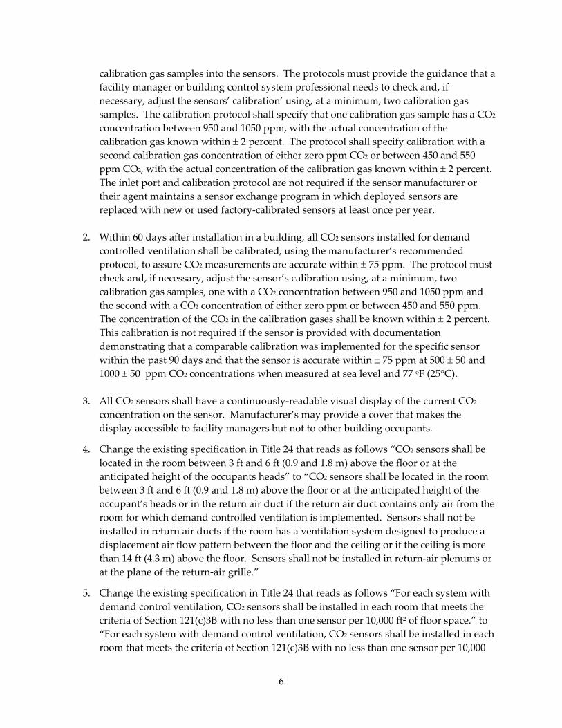
calibration gas samples into the sensors. The protocols must provide the guidance that a facility manager or building control system professional needs to check and, if necessary, adjust the sensors’ calibration’ using, at a minimum, two calibration gas samples. The calibration protocol shall specify that one calibration gas sample has a CO2 concentration between 950 and 1050 ppm, with the actual concentration of the calibration gas known within ± 2 percent. The protocol shall specify calibration with a second calibration gas concentration of either zero ppm CO2 or between 450 and 550 ppm CO2, with the actual concentration of the calibration gas known within ± 2 percent. The inlet port and calibration protocol are not required if the sensor manufacturer or their agent maintains a sensor exchange program in which deployed sensors are replaced with new or used factory-calibrated sensors at least once per year.

2. Within 60 days after installation in a building, all CO2 sensors installed for demand

controlled ventilation shall be calibrated, using the manufacturer’s recommended protocol, to assure CO2 measurements are accurate within ± 75 ppm. The protocol must check and, if necessary, adjust the sensor’s calibration using, at a minimum, two calibration gas samples, one with a CO2 concentration between 950 and 1050 ppm and the second with a CO2 concentration of either zero ppm or between 450 and 550 ppm. The concentration of the CO2 in the calibration gases shall be known within ± 2 percent. This calibration is not required if the sensor is provided with documentation demonstrating that a comparable calibration was implemented for the specific sensor within the past 90 days and that the sensor is accurate within ± 75 ppm at 500 ± 50 and 1000 ± 50 ppm CO2 concentrations when measured at sea level and 77 oF (25°C).

3. All CO2 sensors shall have a continuously-readable visual display of the current CO2

concentration on the sensor. Manufacturer’s may provide a cover that makes the display accessible to facility managers but not to other building occupants.

4. Change the existing specification in Title 24 that reads as follows “CO2 sensors shall be located in the room between 3 ft and 6 ft (0.9 and 1.8 m) above the floor or at the anticipated height of the occupants heads” to “CO2 sensors shall be located in the room between 3 ft and 6 ft (0.9 and 1.8 m) above the floor or at the anticipated height of the occupant’s heads or in the return air duct if the return air duct contains only air from the room for which demand controlled ventilation is implemented. Sensors shall not be installed in return air ducts if the room has a ventilation system designed to produce a displacement air flow pattern between the floor and the ceiling or if the ceiling is more than 14 ft (4.3 m) above the floor. Sensors shall not be installed in return-air plenums or at the plane of the return-air grille.”

5. Change the existing specification in Title 24 that reads as follows “For each system with demand control ventilation, CO2 sensors shall be installed in each room that meets the criteria of Section 121(c)3B with no less than one sensor per 10,000 ft² of floor space.” to “For each system with demand control ventilation, CO2 sensors shall be installed in each room that meets the criteria of Section 121(c)3B with no less than one sensor per 10,000

6

ft² of floor space. In addition to stand- alone sensors that measure the CO2 concentration at a single location, measurements may be performed with measurement systems that use tubing, valves, and pumps to measure at multiple indoor locations with a single CO2 sensor if data are available from each location at least once every 10 minutes.”

6. The required types of building spaces for which demand controlled ventilation is required in Title 24 should not be expanded to include general office spaces’ however, demand controlled ventilation should continue to be optional for general office spaces.

7. At this time, Title 24’s specifications pertaining to demand controlled ventilation should

not be modified to allow use of optical people counting, in place of CO2 sensors, to provide the control signal for demand controlled ventilation.

Classroom Ventilation Available limited evidence suggests that lower ventilation rates (VRs) in both offices and schools are associated with increased illness absence (IA). Data were collected on this relationship in California elementary schools.

Longitudinal data during two school years between 2009-2011 on estimated VRs and illness-related absence were collected from 162 classrooms in 28 schools, within three school districts with distinctly different climates: South Coast (SC), with mild winters and warm summers; Bay Area (BA), with mild summers and winters; and Central Valley (CV), with cold winters and hot summers. Selected within each district were schools across a range of socioeconomic levels, and within schools, classrooms in 3rd, 4th, and 5th grades. Both permanent and portable building types were included, and mixed grade and dedicated special education classrooms were excluded. Daily VRs were estimated from real-time indoor carbon dioxide concentrations measured by web-connected sensors in each classroom. School districts provided daily classroom-level absence data and periodic demographic data. Analyses included four summary metrics for VRs, averaging VRs over periods ranging from 3 to 21 days, with a 7-day average the primary a priori metric. Relationships between daily illness absence and VR metrics were estimated separately by districts, in zero-inflated negative binomial models adjusted for selected covariates.

7

Analyses included data from 10 schools and 59 classrooms in SC, with no air-conditioning (AC) and mostly naturally ventilated classrooms; 5 schools and 26 classrooms in BA, with multiple ventilation types; and 9 schools and 51 classrooms in CV, with all AC classrooms. Median daily VRs in L/s per person were, by district, SC, 7.0, BA, 5.1, and CV, 2.6; by building type, permanent classrooms, 6.8, and portable classrooms, 5.0; and by ventilation type, natural, 6.0, mechanical/no AC, 7.6, and AC, 2.8. Mean daily classroom proportion of illness absence ranged from 2.1-2.5 across districts. In adjusted models, for each additional 1 L/s per person of VR, illness absence was almost invariably lower: statistically significantly in SC (1.0-1.3%), non-significantly in BA (1.2-1.5%), CV (0.0-2.0%), and statistically significantly when combined (1.4-1.8%).

All school districts had overall median daily VRs below the Title 24 minimum VR standard of 7.1 L/s per person. Median VRs were 40% lower in portable than permanent buildings and 54% lower in air-conditioned than naturally ventilated classrooms. Although adjusted estimates were only statistically significantly different from the null overall and in the SC district, estimates in all districts showed consistent patterns, with relative decreases in IA for the 7-day averaged VR metric ranging across models from 1.0-1.6% per L/s per person. Strength of associations across models tended to increase as the averaging period for VR increased, rather than peaking for the 7-day metric as hypothesized. The number of available days of valid classroom data for BA and CV districts was substantially lower (56% and 37% lower, respectively) than that for the SC, which may explain the lack of statistical significance despite similar point estimates. These estimates would apply within the VR range observed, approximately 1.4-20.3 L/s per person, most of it above the State guideline. If these relationships were confirmed, an increase in average classroom VRs from 4 to 7.1 L/s per person (from the average in overall California classrooms to the State guideline level) would be associated with at least a 3.4% relative decrease in illness absence. Making this change in all California K-12 schools, based on these findings and other available data, would be associated with a $33M increase to school districts in state funding but only $4.0 M in increased energy costs to districts for ventilation, heating, and cooling. Thus the low VRs excessively in current classrooms, that save energy, may have unrecognized costs of increased health problems and related illness absence among students. Increasing VRs above the recommended minimum levels, up to 20 L/s per person or higher, may further substantially decrease illness absence. If the magnitude of the relationships observed here, and the estimates of costs and benefits are confirmed, it would be advantageous to students, their families, and school districts, and also highly cost effective, to insure that VRs in elementary school classrooms substantially exceed current recommended ventilation guidelines.

Confirming these findings in intervention studies, and investigating feasibility of substantially increasing ventilation rates in California classrooms, are recommended.

8

CHAPTER 1: Introduction

In this report, the term “ventilation, refers to the intentional and accidental supply of outdoor air to a building. Ventilation is necessary to control indoor air concentrations of indoor-generated air pollutants. From an energy efficiency perspective, the amount of ventilation during hot and cold weather should be minimized because ventilation air must often be heated or cooled and dehumidified.

Prior research has shown that, on average, in offices and schools with higher rates of ventilation, the occupants are more satisfied with air quality, have fewer sick-building-syndrome symptoms such as irritation of eyes and nose, and have a slightly higher level of work performance (Fisk et al. 2009; Seppanen et al. 2006; Seppanen et al. 1999; Sundell et al. 2011). Two prior studies have also found lower absence rates in buildings with higher ventilation rates (Milton et al. 2000; Shendell et al. 2004)

The energy use associated with ventilation in commercial buildings has been estimated via simulations of the existing building stock (Benne et al. 2009). An estimated nine percent of energy used in the stock of U.S. commercial buildings is attributable to heating and cooling ventilation air supplied mechanically with fans and through uncontrolled air infiltration through the building envelope. No comparable estimates are available for California’s commercial buildings, but in California the fraction of total building energy attributable to ventilation is likely to be comparable or moderately smaller.

Given the impacts of ventilation on both indoor environmental quality and energy consumption, in the selection of ventilation rates one must strike a balance between these two important concerns. Minimum ventilation standards have been established that specify minimum design ventilation rates for various types of buildings. In California, these minimum ventilation rates are specified in the California Building Energy Efficiency Standards (California Energy Commission 2008) or Title 24 Standards. For most building types, the minimum ventilation standards specify minimum ventilation rates that are the larger of a minimum rate per person and a minimum rate per unit floor area. However, due to a paucity of data the scientific underpinning for current minimum ventilation standards is relatively weak, particularly for buildings other than offices.

One key element of this research project, discussed in Chapter 6, was designed to help fill the gap in knowledge related to minimum ventilation requirements in classrooms. In a large multi-year field study, this research investigated how student absence rates were affected by classroom ventilation rates.

A larger portion of the current research project, discussed in chapters 2-5, focused on a technology for controlling ventilation rates called demand controlled ventilation. The demand controlled ventilation systems investigated are ones that automatically modulate rates of

9

ventilation as occupancy changes. The goal is to avoid excessive ventilation and associated unnecessary energy use when spaces are unoccupied of have a lower than normal occupancy. Demand controlled ventilation systems are most commonly used in spaces with a high and variable occupant density, such as meeting rooms and are required for such spaces in California (California Energy Commission 2008). Demand controlled ventilation is sometimes also used in spaces with a lower but variable occupancy such as general office areas.

Much of the research on demand controlled ventilation in the current project focused on an evaluation of the performance of sensors used to indirectly or directly sense the level of occupancy in a space or building. Other components of the research investigated where sensors should be located within meeting rooms and the potential energy savings from using demand controlled ventilation in general office spaces within California. This research led to a number of specific recommended changes to specifications for demand controlled ventilation in Title 24.

10

CHAPTER 2: Accuracy of CO2 Sensors Used for Demand Controlled Ventilation 2.1. Background People produce and exhale carbon dioxide (CO2) as a consequence of their normal metabolic processes; thus, the concentrations of CO2 inside occupied buildings are higher than the concentrations of CO2 in the outdoor air. The magnitude of the indoor-outdoor concentration difference decreases as the building’s ventilation rate per person increases. If the building has a nearly constant occupancy for several hours and the ventilation rate is nearly constant, the ventilation rate per person can be estimated from the maximum steady state difference between indoor and outdoor CO2 concentrations (ASTM 1998; Persily 1997). For example, under steady conditions, if the indoor CO2 concentration in an office work environment is 700 parts per million above the outdoor concentration, the ventilation rate is approximately 7.5 L/s (15 cfm) per person (ASHRAE 2007). In many buildings, occupancy and ventilation rates are not stable for sufficient periods to allow indoor CO2 concentrations to equilibrate sufficiently for accurate determinations of ventilation rates from CO2 data; however, CO2 concentrations remain an approximate, easily measured, and widely used proxy for ventilation rate per occupant. The difference between the indoor and outdoor CO2 concentration is also a proxy for the indoor concentrations of other occupant-generated bioeffluents, such as body odors (Persily 1997).

Epidemiological research has found that indoor CO2 concentrations are useful in predicting human health and performance. Many studies have found that occupants of office buildings with a higher difference between indoor and outdoor CO2 concentration have, on average, increased sick building syndrome health symptoms (Seppanen et al. 1999). In a study within a jail, higher CO2 concentrations were associated with increased respiratory disease (Hoge et al. 1994) and higher CO2 concentrations in schools have been associated with increased student absence (Shendell et al. 2004) and office worker absence (Milton et al. 2000). Additionally, a recent study (Shaughnessy et al. 2006) found poorer student performance on standardized academic performance tests correlated with increased CO2 in classrooms and Wargocki and Wyon (2007) found that students performed various school-work tasks less rapidly when the classroom CO2 concentration was higher.

In a control strategy called demand controlled ventilation (Emmerich and Persily 2001; Fisk and de Almeida 1998), CO2 sensors, sometimes called CO2 transmitters, are deployed in commercial buildings to obtain CO2 data that are used to automatically modulate rates of outdoor air supply. The goal is to keep ventilation rates at or above design requirements but also to adjust the outside air supply rate with changes in occupancy in order to save energy by avoiding over-ventilation relative to design requirements. Demand controlled ventilation is most often used in spaces such as meeting rooms with variable and sometimes dense occupancy. Some buildings use CO2 sensors just to provide feedback about ventilation rates to the building operator, without automatic modulation of ventilation rates based on the measured CO2

11

concentrations. In nearly all cases, each of the CO2 sensors deployed for demand controlled ventilation measure CO2 concentrations at a single indoor location. In this report, these sensors are referred to as “single-location” CO2 sensors. A small number of buildings utilize CO2 sensors connected to tubing, valves, and pumps for measurements of CO2 concentrations as multiple indoor locations as well as outdoors. In this report, these systems are referred to as “multi-location” CO2 measurement systems.

Reviews of the research literature on demand controlled ventilation (Apte 2006) (Emmerich and Persily 2001; Fisk and de Almeida 1998) indicate a significant potential for energy savings, particularly in buildings or spaces with a high and variable occupancy. Based on modeling (Brandemuehl and Braun 1999), cooling energy savings from applications of demand controlled ventilation are as high as 20%. However, there have been many anecdotal reports of poor CO2

sensor performance in actual applications of demand controlled ventilation. Also, pilot studies of sensor accuracy in California buildings indicated substantial error in the measures made by many of the evaluated CO2 sensors (Fisk et al. 2007).

Based on the prior discussion, there is a good justification for monitoring indoor CO2 concentrations and using these concentrations to modulate rates of outdoor air supply. However, this strategy will only be effective if CO2 sensors have a reasonable accuracy in practice.

This chapter provides the results of research performed to evaluate the in-situ accuracy of CO2 measurement systems used for CO2 demand controlled ventilation and, to the degree possible via analyses of the data, to determine how accuracy varies with sensor age and sensor technical features. The primary focus was the accuracy of the most commonly used type of CO2 sensor that measures CO2 at a single indoor location. A small preliminary evaluation of CO2 measurements made with multi-location sampling systems was also performed to provide an initial indication of the potential of CO2 monitoring using more expensive, and thus potentially more stable and accurate, CO2 sensors coupled with multi-location sampling systems. Systems that employ multi-location sampling equipment to measure CO2 concentrations at multiple locations using the same CO2 sensor are much less common than distributed single-location sensors. Multi-location systems have advantages and disadvantages. Advantages include the use of one sensor to measure at multiple locations potentially reducing total sensor costs, the potential to spend more to obtain a higher quality sensor if it is used for multiple-location measurements, the ease of calibrating a single or small number of sensors relative to calibrating many sensors, and the potential to include an outdoor CO2 measurement in each building, or preferably, with each CO2 sensor. Also, the multi-location sampling system may, in some cases, be usable to measure contaminants other than CO2. Disadvantages include the need for a multi-location sampling systems of tubing, valves, and pumps, the potential for leakage-related errors with multi-location sampling system, the need for a sample pump, and the reduced frequency in which CO2 concentration data are available from each location. In an additional task, spatial variability of CO2 concentrations in meeting rooms was evaluated to provide information to aid selection of sensor locations.

12

One additional component of the research was an evaluation of a small sample of single-location CO2 sensors that had large errors, with the goal of identifying causes of sensor inaccuracy.

2.2. Methods

2.2.1. Field studies of single-location CO2 sensor performance The research on single-location CO2 sensors, hereinafter called “sensors,” was performed in two phases. The pilot study phase supported by the U.S. Department of Energy evaluated the performance of 43 CO2 sensors located in nine buildings in California. The second study phase supported by the California Energy Commission evaluated the performance of 165 sensors from 25 buildings in California. This report presents and analyzes the data from both study phases, with a total of 208 sensors located in 34 buildings. Two different protocols were employed to assess the accuracy of the CO2 sensors. When possible, bags of primary standard CO2 calibration gases were used to evaluate sensor performance at five CO2 concentrations from 230 to 1780 parts per million (ppm). This procedure is referred to as a multi-concentration calibration check. Based on the specifications of the calibration gas supplier and the protocols employed, the calibration gas concentrations were known within about 5%. In the multi-concentration calibration checks, the CO2 sensors located in buildings sampled each of the calibration gas mixtures. The CO2 concentrations reported on the computer screen of the building’s data acquisition system or on the CO2 sensor display, or when possible at both locations, were recorded. The data obtained were processed to obtain a zero offset error and slope or sensor gain error using a least-squares linear regression of measured CO2 concentration versus “true” reference CO2 concentration. If a sensor agreed exactly with the “true” concentration, then the zero offset error would be zero and the slope equal unity. However, an offset error of 50 ppm would indicate that the sensor would read 50 ppm high at a concentration of 0 ppm, and 50 ppm high at all CO2 concentrations if the sensor’s slope is unity. A slope of 0.8 would indicate that slope of the line of reported concentration plotted versus true concentration is 0.8. The multi-concentration calibration process also yielded errors at each of the calibration gas concentrations. The three calibration gas concentrations used that are most representative of the CO2 concentrations typically encountered in buildings are 510, 760, and 1010 ppm. The multi-concentration calibrations were performed when the CO2 sensors had an inlet port and the sensor had a concentration display or the building operator was able and willing to program the data acquisition system so that data were provided with sufficient frequency (e.g., every several minutes) to make a multipoint calibration possible with calibration gas bags of a practical volume. This type of performance test was completed for 90 sensors from 19 buildings. When a multi-concentration calibration check was not possible, single-concentration calibration checks of the building’s CO2 sensors were performed using a co-located and calibrated reference CO2 instrument. The protocol was very simple. A calibrated research-grade CO2 instrument

13

was taken to the building where its calibration was checked with samples of primary standard calibration gases. The reference instrument was placed so that it sampled at the same location as the building’s CO2 sensor. Data from the reference instrument was logged over time. CO2 concentrations reported on the sensor’s display or the building’s data acquisition system’s screen, or at both locations, were recorded manually. The data were processed to obtain an absolute error, equal to the CO2 concentration reported by the building’s data acquisition system minus the true CO2 concentration. This type of sensor performance check was completed for 118 sensors located in 24 buildings, including single-concentration calibration checks of sensors for which multi-concentration calibrations were also completed. One limitation of the single-concentration calibration data is that much of the data were obtained with CO2 concentrations below 500 ppm, with an average concentration of 466 ppm. For subsequent analyses, the data from the single-concentration calibration checks was combined with the data obtained using the 510 ppm calibration gas in the multi-concentration calibration checks of sensors. When both types of data were available, the data obtained with the 510 ppm calibration gas was used in analyses. The resulting data set is called the “combined dataset” and contained data from 207 sensors in 34 buildings1. The reference CO2 instrument used for the single point calibrations has an automatic zero feature and is calibrated with a span gas. The rated accuracy is “better than 1% of span concentration” but is limited by the accuracy of the calibration gas mixture. In this study, the span gas concentration was 2536 ppm and rated at ± 2% accuracy. Multi-concentration calibration checks of this reference instrument were also performed using precision dilutions of the span gas during field site visits. Figure 2.2.1 shows an example of the deviations between the reference instrument output and the concentration of CO2 in the diluted span gas. The deviations range from approximately +1% to – 2%. To further evaluate the accuracy of measurements with the reference instrument, it was used to measure the CO2 concentration in nine additional calibration gas mixtures, all distinct from the span gas routinely used for instrument calibration checks. As shown in Figure 2.2.2, the reference instrument output deviated from the reported calibration gas concentration by approximately -1% to -5%. Given these data, the uncertainty in CO2 concentration measurements made with the reference instrument is estimated to be 5% or less.

1 One of the multipoint sensor calibrations lacked data at 510 ppm for combination with the single point data.

14

Figure 2.2.1: Example of measurement errors of reference CO2 instrument when measuring precise dilutions of the span gas.

-2%

-2%

-1%

-1%

0%

1%

0 20 40 60 80 100Calibration Gas Concentration (% of 2536 ppm)

Mea

sure

men

t Err

or

Errors in measurement of precise dilutions of a 2536 ppm

CO2 calibration gas

Figure 2.2.2: Errors in measuring the concentration of nine CO2 calibration gases with the reference CO2 instrument.

-6%

-5%

-4%

-3%

-2%

-1%

0%

0 1000 2000 3000 4000 5000 6000Calibration Gas Concentration (ppm)

Mea

sure

men

t Err

or

Errors in measurement of nine calibration gases with reference CO2 instrument, all were distinct from the span gas used to calibrate the reference CO2 instrument

15

All of the CO2 sensors evaluated were non dispersive infrared sensors. The sensors generally have a default measurement range of zero to 2000 ppm, although in some cases other ranges can be selected. Nearly all sensors sampled via diffusion, i.e., had no sample pump. The manufacturers’ accuracy specifications translate into maximum errors of ± 40 ppm to ± 100 ppm at a concentration of 1000 ppm if the sensor range is zero to 2000 ppm. The manufacturers’ recommended calibration frequency ranged from every six to 12 months for older products to “never needs a calibration under normal conditions,” with a five year recommended calibration interval being common. Some sensors use two lamps or two wavelengths of infrared energy in a process to correct for sources of potential drift in sensor calibration, e.g., to correct for diminished lamp infrared energy output (National Buildings Controls Information Program 2009). For analysis purposes, sensors were classified into the following four design categories: single lamp, single wavelength; dual lamp, single wavelength; single lamp, dual wavelength; or unknown when product literature did not specify the design. In this classification scheme, “lamp” refers to the infrared source(s) and “wavelength” refers to the wavelength(s) of infrared energy detected by the sensor’s detector. Based on product literature, some sensors perform a self-calibration or auto-calibration. In many instances, this self calibration is an “automated background calibration” process in which the sensor’s calibration is automatically reset based on a complex algorithm and the lowest sensor responses encountered during a prior period. This automatic background calibration process assumes that the lowest encountered CO2 concentration is approximately 400 ppm; i.e., that the CO2 concentration at the sensor location drops to the outdoor air CO2 concentration. However, product literature for some sensors simply refers to a “self calibration” without providing details, and for many sensors the product literature does not indicate whether or not there is a self calibration feature.

For analyses of how various sensor features related with sensor accuracy, sensors were assigned a manufacturer code number (1 – 10 plus 11 for a few sensors locked in a box with an unknown manufacturer), a sensor design code, a self calibration code, and a sensor age. Sensors were assigned the sensor design code based on a review of product literature. The sensor design code numbers and corresponding sensor designs were as follows: 1 = known single lamp single wavelength; 2 = suspected single lamp single wavelength; 3 = dual lamp single wavelength; 4 = single lamp dual wavelength; 5 = unknown. For many sensors, the sensor design code could not be determined due to, for example, the lack of design information on product literature. Sensors were also grouped into the following two categories: sensors in which product literature refers to a self-calibration feature (normally automatic baseline control) and other sensors. This categorization is crude. The designs of dual lamp and dual wavelength sensors are intended to automatically correct for sources of error which could be considered a form of self-calibration, but normally the product literature for these sensors did not refer to a self-calibration.

Facility managers were asked about the sensor age; i.e., the time elapsed since sensor installation in the building, the CO2 concentration setpoint used to trigger an increase in ventilation rate, the sensor calibration history, and the sensor cost. In general they provided only estimates of sensor ages, some did not know the setpoint, and almost none provided any specific information on costs. No facility manager reported that they had calibrated the sensors

16

since their initial installation in the building. For analysis purposes, an age of 0.5 years was assigned for sensors characterized by the facility manager as “new.” When a facility manager indicated that a sensor was more than “n” years old, “n” was assigned as the sensor age.

Bivariate statistical analyses were performed using the anova and regress commands in STATA version 10. For the multi-concentration calibration checks, outcomes were the absolute value of error at 760 and 1010 ppm. For the combined single-concentration and multi-concentration calibration data, the outcome was absolute error at the concentration encountered or at 510 ppm. Outcome variables were log-transformed to produce normally-distributed residuals with a constant variance, as is required for valid inference from ANOVA and linear regression models. Groups with fewer than 11 observations were excluded from the analysis. Pairwise comparisons of groups were performed using the Tukey wholly significant difference method with α=0.05. This method makes it more difficult to reject the null hypothesis in each individual pairwise comparison. Additionally, sensor types were analyzed using both the individual types (1-5) and groupings of type 1 and 2 versus types 3, 4, and 5. Sensor age was treated as a categorical variable with groups 0-1 year, 1.5-3 years, 3.5-5 years, and 5-7 years for the combined dataset and groups 0-1 year, 1.5-3 years, and 3.5-7 years for the multi-concentration dataset. Linear regression was performed on the log-transformed year, using the robust standard errors option.

Multivariate statistical analyses were performed using the regress command with the robust standard error option specified for both the combined dataset and the multi-concentration dataset on its own. All outcomes (absolute error, absolute error at 760 ppm, absolute error at 1010 ppm) were log-transformed in order to meet the assumptions for regression. A dummy variable was created for each sensor grouping category with categories containing very few observations combined into an “other” category. Sensor age was introduced as a categorical measure with categories defined as in the bivariate analysis.

The sensor performance checks, for single-location sensors, were all performed in commercial buildings located in California, selected without consideration of building age or type of CO2 sensor. The buildings were used for healthcare, education, software industry, judicial, library, utility, corrections, law enforcement, museum, entertainment, retail, and state and federal and private office applications. There were ten brands of CO2 sensors2 and multiple model types of some brands.

2.2.2. Evaluation of faulty single-location CO2 sensors Nine of the single-location CO2 sensors that had large measurement errors (range 255 – 858 ppm, average 458 ppm) based on the assessments described in Section 2.2.1 were obtained for further evaluation in the laboratory. To obtain the sensors, facility managers were offered a new replacement sensor if they would provide a specified existing sensor for evaluation. In the prior field studies, these sensors had received only a single-concentration calibration check using a co-located and calibrated reference CO2 instrument. Sensors from four different

2 Some of the manufacturers market sensors from other manufacturers.

17

manufacturers and with different design features were obtained. The following evaluation protocol was implemented. The first step in the evaluation was designed to evaluate the sensor responses at multiple CO2 concentrations after 11 days of sensor operation in a highly ventilated room with outdoor air CO2 concentrations. After this conditioning period, during which “automated background calibration” software may have corrected some of the sensor calibrations, CO2 concentrations in the room were normally equal to the outdoor air concentration. Periodically, pure CO2 was added to room air in amounts sufficient to increase concentrations to approximately 500, 700, 1000, and 1500 ppm and the air in the room was mixed using fans. A reference CO2 instrument continuously monitored CO2 concentrations within the room. The output signal of the sensors was logged continuously. The resulting data were analyzed to determine measurement errors and whether they were stable. The second step was to implement the manufacturer’s recommended sensor calibration protocols when possible and then to reassess sensor performance using the protocols described in the previous paragraph. For two sensors, the manufacturer provided no calibration protocol. Four sensors had no response or only a very small response to changing CO2 concentrations. One sensor had an output signal problem that caused the data acquisition system to fail. Thus, a manufacturer’s recommended calibration could only be implemented for two sensors. For one of these sensors, the manufacturer’s protocol utilized only a calibration gas with no CO2. For the other sensor, the manufacturer’s protocol utilized both a 0 ppm CO2 calibration gas and a 2000 ppm CO2 calibration gas. The third evaluation step was to remove the sensor covers and have an electronics expert inspect each sensor for visual evidence of any electronics component failures. Based on a discussion with the research director of a sensor company and an examination of the limited technical information available from sensor manufacturers it was determined that detailed studies of the electronic performance of sensors was not feasible. Measurement of the output of the IR lamps was also not feasible as no lamp output data or evaluation protocols were available and most sensor lamps were inside optical cells that could not be opened non-destructively. In the final step in the evaluations, the optical cells of each sensor were opened and the cells visually inspected under low power magnification for signs of soiling or corrosion of the cell surfaces.

2.2.3. Pilot evaluation of CO2 demand controlled ventilation with multi-location sampling systems The accuracy of multi-location CO2 measurement systems was evaluated in two buildings. The same manufacturer provided the multi-location systems used in both buildings. There are two additional manufacturers of multi-location CO2 measurement systems, but one has only a few

18

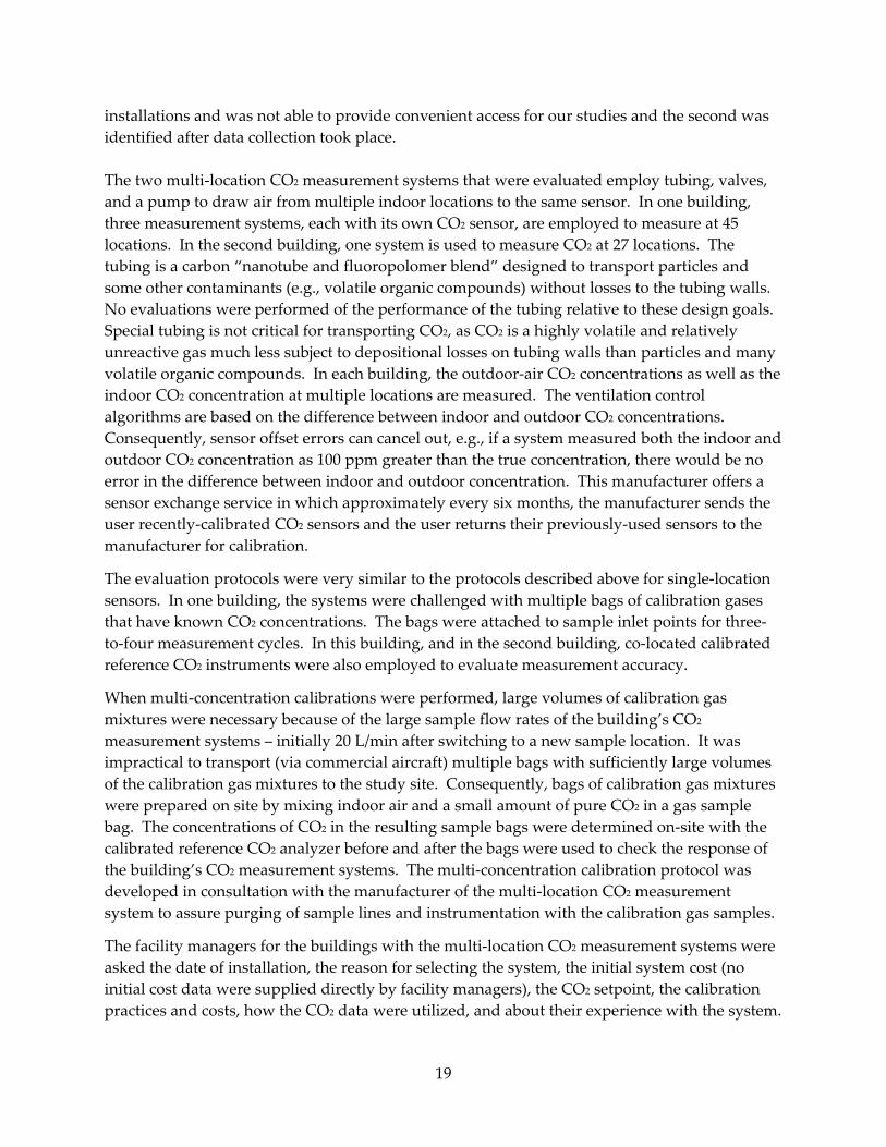
installations and was not able to provide convenient access for our studies and the second was identified after data collection took place. The two multi-location CO2 measurement systems that were evaluated employ tubing, valves, and a pump to draw air from multiple indoor locations to the same sensor. In one building, three measurement systems, each with its own CO2 sensor, are employed to measure at 45 locations. In the second building, one system is used to measure CO2 at 27 locations. The tubing is a carbon “nanotube and fluoropolomer blend” designed to transport particles and some other contaminants (e.g., volatile organic compounds) without losses to the tubing walls. No evaluations were performed of the performance of the tubing relative to these design goals. Special tubing is not critical for transporting CO2, as CO2 is a highly volatile and relatively unreactive gas much less subject to depositional losses on tubing walls than particles and many volatile organic compounds. In each building, the outdoor-air CO2 concentrations as well as the indoor CO2 concentration at multiple locations are measured. The ventilation control algorithms are based on the difference between indoor and outdoor CO2 concentrations. Consequently, sensor offset errors can cancel out, e.g., if a system measured both the indoor and outdoor CO2 concentration as 100 ppm greater than the true concentration, there would be no error in the difference between indoor and outdoor concentration. This manufacturer offers a sensor exchange service in which approximately every six months, the manufacturer sends the user recently-calibrated CO2 sensors and the user returns their previously-used sensors to the manufacturer for calibration.

The evaluation protocols were very similar to the protocols described above for single-location sensors. In one building, the systems were challenged with multiple bags of calibration gases that have known CO2 concentrations. The bags were attached to sample inlet points for three-to-four measurement cycles. In this building, and in the second building, co-located calibrated reference CO2 instruments were also employed to evaluate measurement accuracy.

When multi-concentration calibrations were performed, large volumes of calibration gas mixtures were necessary because of the large sample flow rates of the building’s CO2 measurement systems – initially 20 L/min after switching to a new sample location. It was impractical to transport (via commercial aircraft) multiple bags with sufficiently large volumes of the calibration gas mixtures to the study site. Consequently, bags of calibration gas mixtures were prepared on site by mixing indoor air and a small amount of pure CO2 in a gas sample bag. The concentrations of CO2 in the resulting sample bags were determined on-site with the calibrated reference CO2 analyzer before and after the bags were used to check the response of the building’s CO2 measurement systems. The multi-concentration calibration protocol was developed in consultation with the manufacturer of the multi-location CO2 measurement system to assure purging of sample lines and instrumentation with the calibration gas samples.

The facility managers for the buildings with the multi-location CO2 measurement systems were asked the date of installation, the reason for selecting the system, the initial system cost (no initial cost data were supplied directly by facility managers), the CO2 setpoint, the calibration practices and costs, how the CO2 data were utilized, and about their experience with the system.

19

Because facility managers did not provide cost data, estimates of installed costs were obtained from the manufacturer.

2.2.4. Pilot evaluation of spatial variability of CO2 concentrations in meeting rooms The field studies included multipoint measurements of CO2 concentrations in six meeting spaces suitable for demand controlled ventilation. Concentrations of CO2 were measured once per minute at various locations and heights on meeting room walls and in return air grilles. Figure 2.2.3 shows a schematic of one of three measurement systems, each with the capability for measurements at three locations. Samples were drawn continuously from each sample point. Sequential activation of the three-way solenoid valves for a 20 second periods directed air from specific sample points to the CO2 instrument, which is the same type of instrument described above as the reference CO2 instrument. When a solenoid valve was not activated, the sample stream was vented. The continuous sampling through the sample inlet tubes maintained the tubes purged so that data could be collected at high frequency. The system was calibrated using bags of primary standard calibration gas mixtures attached at the inlet end of the sample lines. The output of the CO2 instrument was logged continuously and reported every two seconds. Approximately 10 - 12 seconds after activation of a solenoid valve, the output signal from the CO2 instrument was stable if the concentration at the inlet line of the sample tube was stable, indicating purging of the sample hardware downstream of the three-way valve and equilibration of the instrument response. The output signal from the subsequent sample period was converted to the CO2 concentration using the calibration data for the CO2 instrument. The system was tested before use and the CO2 instrument was calibrated at each installation location.

Figure 2.2.3: Schematic representation of one of three systems employed to rapidly measure indoor carbon dioxide concentrations at three indoor locations per system.

Sample Point

Sample Point

Sample Point

CO2 Instrument

Pumps Three Way Solenoid Valves

Sample vent

20

The three systems provided measurements at nine locations. In general, the measurement locations included a location on each wall at approximately a 1.5 m (5.0 ft) above the floor (typical of the heights at which sensors were installed in field settings), inside one or two return grilles, at lower and higher heights (typically 0.4 and 1.7 m or 1.5 and 5.5 ft) at one of the walls, and a supply air register. In some spaces, the measurement heights had to be adjusted to accommodate wall mounted equipment, such as white boards or display screens. Based on the data, one of the supply airstreams may have contained only recirculated room air. In one meeting room, many chairs were placed immediately adjacent to parts of some walls and sample locations were selected away from these chairs to reduce the impacts of exhaled air with very high CO2 concentrations.

2.3. Results

2.3.1 Field studies of single-location CO2 sensor performance 2.3.1.1 Multi-concentration calibration checks of single-location sensors Table 2.3.1 provides the primary results from the multi-concentration calibration checks of 90 sensors. The first row of data provides the results of evaluations of all 90 sensors and subsequent rows provide results for overlapping subsets of the sensors. Data from each sensor is provided in Appendix A. For the full set of sensors, the average slope was 0.97 and the average of the absolute value of zero offsets was 79 ppm. The averages of the absolute values of error were 118 ppm (16%) and 138 ppm (14%), at concentrations of 760 and 1010 ppm, respectively. The calibration data are generally well fit by a straight line as indicated by the high values of R2. For subsets of the full set of sensors, the accuracy is often significantly better or worse than for the full set of sensors. For example, sensors from Manufacturer 4 and 5, sensors with the Type 1 design (single lamp and single wavelength) or with Type 2 design (suspected single lamp and single wavelength design), and sensors with a manufacturer-reported self-calibration system tend to have a better-than-average average accuracy. However, the variability in sensor accuracy within each category is large, as indicated by standard deviations that are often comparable to or larger than the average error for the category.

Figure 2.3.1 provides frequency distributions for the slope, zero offset, error at 760 ppm, and error at 1010 ppm that clearly illustrate the high variability in accuracy. In each case, the error parameters are approximately normally distributed. Figure 2.3.2 shows how error at the 760 and 1010 ppm concentration varies with manufacturer code and the figure provides the average absolute value of error for each category. Sensors from Manufacturers 4 and 5 have substantially lower average absolute value errors at 1010 ppm, and sensors from Manufacturer 2 also have the lowest average absolute value error at 760 ppm. Figure 2.3.3 shows that the lowest average absolute value errors are associated with sensor design type 1 (single lamp single wavelength) and, at 1010 ppm, also with sensor design type 2 (suspected single lamp single wavelength design). There is a substantial overlap in the sensors within these categories associated with better accuracy; i.e., the sensors from manufacturers 4 and 5 generally had a single lamp single wavelength design and their literature refers to a self-calibration procedure.

21

As illustrated by the frequency distribution plots in Figure 2.3.1, a significant fraction of sensors had errors substantially larger than 100 ppm. For example, at 1010 ppm, 19% of sensors had an error greater than 200 ppm and13% of sensors had errors greater than 300 ppm.

Error is plotted versus sensor age in Figure 2.3.4. Given the large standard deviations, indicated by the error bars, there is no clear trend in error with sensor age in the multi-concentration calibration data.

Table 2.3.2 provides the proportion of sensors in various categories that had errors greater than ±75 ppm and greater than ±100 ppm at calibration gas concentrations of 760 and 1010 ppm. For the full set of sensors subject to the multi-concentration calibration checks, at 1010 ppm, 40% and 31% of sensors had errors greater than ±75 ppm and ±100 ppm, respectively. At 760 ppm, 47% of sensors had errors greater than ±75 ppm and 37% of sensors had errors greater than ±100 ppm. These proportions varied substantially with manufacturer, sensor design type, and with versus without a self-calibration procedure. Sensors with type 1 (single lamp single wavelength) and type 2 (suspected single lamp single wavelength) designs and those with a self-calibration performed best at 1010 ppm with 12% to 14% having an error greater than ±100 ppm and just over 20% having an error exceeding ±75 ppm. However, at 760 ppm, 36% to 48% of these same sensors had errors exceeding the same criteria.

22

Table 2.3.1: Primary results of the multi-concentration calibration checks of 90 sensors.

Sensor Group

___

No. Sen-sors___

Slope Linearity R2 Zero Offset Error at 760

ppm Error at

1010 ppm ABV (Zero

Offset) ABV (Error at

760 ppm) ABV (Error at

1010 ppm) Avg SD Avg SD Avg SD Avg SD Avg SD Avg SD Avg SD Avg SD

---- ---- ---- ---- ppm ppm ppm ppm ppm Ppm ppm ppm ppm ppm ppm ppm

all sensors 90 0.97 0.28 0.97 0.10 14 113 -26 200 -9 258 79 83 118 163 138 218 Manu. 1 4 0.71 0.48 0.79 0.42 -9 36 -235 360 -324 478 27 21 247 349 342 461 Manu. 2 2 0.35 0.08 0.72 0.06 -95 26 -737 27 -774 38 95 26 737 27 774 38 Manu. 4 29 0.91 0.12 0.99 0.02 66 98 1 72 -21 98 88 78 49 52 69 72 Manu. 5 33 0.97 0.09 0.99 0.02 12 84 -37 131 -4 124 59 60 100 91 70 102 Manu. 6 5 1.01 0.21 1.00 0.00 43 26 51 174 61 239 43 26 93 151 134 198 Manu. 7 16 1.19 0.49 0.98 0.03 -67 166 64 252 153 385 124 127 179 184 281 299 Type 1 26 0.95 0.06 1.00 0.00 30 76 16 71 10 80 64 49 49 53 53 59 Type 2 17 0.98 0.06 0.98 0.01 -28 45 -126 35 -45 53 45 26 126 35 49 49 Type 3 2 0.41 0.59 0.57 0.59 -25 43 -476 396 -650 507 30 35 476 396 650 507 Type 4 27 1.06 0.42 0.98 0.03 1 168 34 198 68 318 116 120 125 156 204 250 Type 5 18 0.90 0.25 0.97 0.09 57 95 -32 296 -48 325 80 75 156 250 190 265 No Self-Cal. 39 0.99 0.42 0.95 0.15 8 152 -17 288 1 386 101 112 176 226 250 291 Self-Cal. 51 0.95 0.07 0.99 0.01 19 73 -34 88 -17 72 62 43 73 58 53 52 Age 0 – 1 yr 26 1.09 0.43 0.98 0.03 7 166 81 181 121 307 109 123 119 157 204 258 Age 1.5 - 3 yr 23 0.98 0.06 0.98 0.02 -15 47 -91 69 -32 55 42 25 99 55 46 44

Age 3.5 - 7 yr 37 0.94 0.10 1.00 0.00 45 94 2 132 -11 149 82 65 75 108 88 120

Key: ABV = absolute value, Avg = average, Cal. = calibration, Manu = manufacturer, SD = standard deviation, Type 1 is single lamp single wavelength, Type 2 is suspected single lamp single wavelength, Type 3 is dual lamp single wavelength; Type 4 is single lamp dual wavelength; Type 5 = unknown type

23

Figure 2.3.1: Frequency distributions of key results from the multi-concentration calibration checks.

Figure 2.3.2: Errors at 760 and 1010 ppm versus manufacturer code from multi-concentration calibration checks.

05

1015202530354045

0

0.4

0.7 1

1.3

1.6

1.9

2.4 3

Calibration Slope / Correct Slope

Freq

uenc

y

Average = 0.97

0

5

10

15

20

25

-300

-200

-100 0

100

200

300

Zero Offset Error (ppm)

Freq

uenc

y

Average = 14Average Absolute

Value = 79

05

101520

2530

-300

-200

-100 0

100

200

300

Error at 761 ppm (ppm)

Freq

uenc

y

Average = - 26Average

Absolute Value = 118

05

101520253035

-300

-200

-100 0

100

200

300

Error at 1014 ppm (ppm)

Freq

uenc

yAverage = - 9

Average Absolute

Value = 138

247

737

49 100 93 179

-1000-800-600-400-200

0200400600800

1000

0 1 2 3 4 5 6 7 8Sensor Manufacturer Code

Erro

r (pp

m)

average

averageabsolute value

at 760 ppm

342

774

69 70 134281

-1500

-1000

-500

0

500

1000

1500

0 1 2 3 4 5 6 7 8Sensor Manufacturer Code

Erro

r (pp

m)

average

averageabsolute value

at 1010 ppm

24

Figure 2.3.3: Errors at 760 and 1010 ppm versus sensor design type from multi-concentration calibration checks.

Figure 2.3.4: Errors at 760 and 1010 ppm versus sensor age from multi-concentration calibration checks. The error bars represent one standard deviation in the error.

0

50

100

150

200

250

300

350

0 - 1 1.5 - 3 3.5 - 7

Sensor Age (years)

Ave

rage

Err

or (p

pm) At 760 ppm

At 1010 ppm

49 126

476

125 156

-1000-800-600-400-200

0200400600800

0 1 2 3 4 5 6Sensor Type Code

Erro

r (pp

m)

average

average absolutevalue

at 760 ppm

53 49

650

204 190

-1200-900-600-300

0300600900

1200

0 1 2 3 4 5 6Sensor Type Code

Erro

r (pp

m)

average

averageabsolute value

at 1010 ppm

25

Table 2.3.2: Proportions of CO2 sensors in various sensor categories with errors greater than ±75 and ±100 ppm in the multi-concentration calibration checks.

Sensor Group No. of. Sensors --------At 760 ppm------- --------At 1010 ppm-----

Proportion with error > ±75 ppm

Proportion with error > ±100ppm

Proportion with error > ±75 ppm

Proportion with error > ± 100ppm

all sensors 90 0.47 0.37 0.40 0.31 Manu. 1 4 0.50 0.50 0.50 0.50 Manu. 2 2 1.00 1.00 1.00 1.00 Manu. 4 29 0.21 0.14 0.37 0.27 Manu. 5 33 0.61 0.48 0.24 0.18 Manu. 6 5 0.20 0.20 0.20 0.20 Manu. 7 16 0.69 0.50 0.75 0.56 Type 1 26 0.20 0.12 0.27 0.12 Type 2 17 0.88 0.88 0.12 0.12 Type 3 2 1.00 1.00 1.00 1.00 Type 4 27 0.52 0.33 0.67 0.52 Type 5 18 1.00 0.22 1.00 0.39

Type 1 - 2 43 0.48 0.43 0.21 0.12 Type 3 - 5 47 0.47 0.32 0.57 0.49

No Self-Cal. 39 0.54 0.38 0.64 0.54 Self-Cal. 51 0.42 0.36 0.22 0.14

Manu = manufacturer; Cal = calibration, Type 1 is single lamp single wavelength, Type 2 is suspected single lamp single wavelength, Type 3 is dual lamp single wavelength; Type 4 is single lamp dual wavelength; Type 5 = unknown type

2.3.1.2 Combined data set Table 2.3.3 provides the primary results of data from the single-concentration calibration checks combined with the data from challenging sensors with a 510 ppm calibration gas in the multi-concentration calibration checks. Data for individual sensors are provided in Appendix A. For the full set of 207 sensors, the average error was 60 ppm and the average of the absolute value of error was 154 ppm. The standard deviations associated with these two averages were high, 263 and 222 ppm, respectively. Considering only categories with greater than 10 sensors, average absolute value of error was smallest for Manufacturer 5 (58 ppm) and for sensor design types 1 and 2 (66 and 24 ppm, respectively). Again, sensors with a self-calibration designated in product literature had a lower average absolute value error (83 versus 218 ppm). The average of absolute value of error increased with sensor age. However, the standard deviations in the errors in each category were generally larger than the average errors.

26

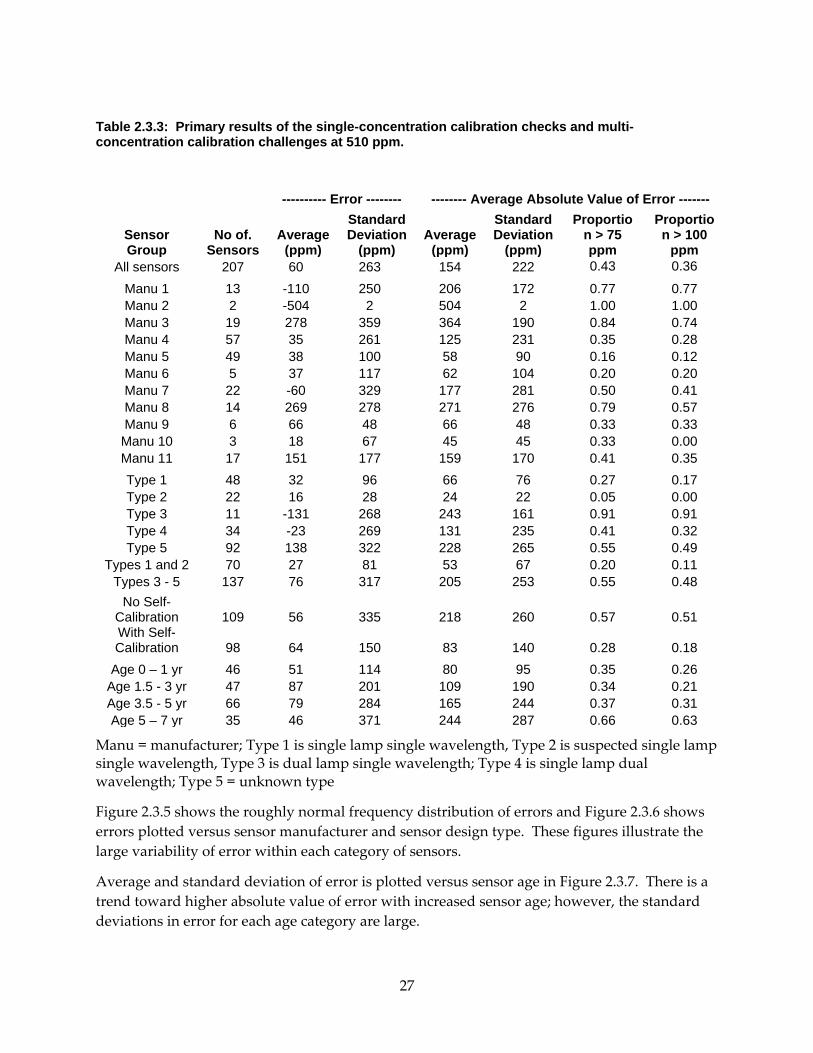
Table 2.3.3: Primary results of the single-concentration calibration checks and multi-concentration calibration challenges at 510 ppm.

Sensor Group

No of. Sensors

---------- Error -------- -------- Average Absolute Value of Error -------

Average (ppm)

Standard Deviation

(ppm) Average

(ppm)

Standard Deviation

(ppm)

Proportion > 75 ppm

Proportion > 100

ppm All sensors 207 60 263 154 222 0.43 0.36

Manu 1 13 -110 250 206 172 0.77 0.77 Manu 2 2 -504 2 504 2 1.00 1.00 Manu 3 19 278 359 364 190 0.84 0.74 Manu 4 57 35 261 125 231 0.35 0.28 Manu 5 49 38 100 58 90 0.16 0.12 Manu 6 5 37 117 62 104 0.20 0.20 Manu 7 22 -60 329 177 281 0.50 0.41 Manu 8 14 269 278 271 276 0.79 0.57 Manu 9 6 66 48 66 48 0.33 0.33 Manu 10 3 18 67 45 45 0.33 0.00 Manu 11 17 151 177 159 170 0.41 0.35

Type 1 48 32 96 66 76 0.27 0.17 Type 2 22 16 28 24 22 0.05 0.00 Type 3 11 -131 268 243 161 0.91 0.91 Type 4 34 -23 269 131 235 0.41 0.32 Type 5 92 138 322 228 265 0.55 0.49

Types 1 and 2 70 27 81 53 67 0.20 0.11 Types 3 - 5 137 76 317 205 253 0.55 0.48

No Self-Calibration 109 56 335 218 260 0.57 0.51 With Self-Calibration 98 64 150 83 140 0.28 0.18

Age 0 – 1 yr 46 51 114 80 95 0.35 0.26 Age 1.5 - 3 yr 47 87 201 109 190 0.34 0.21 Age 3.5 - 5 yr 66 79 284 165 244 0.37 0.31 Age 5 – 7 yr 35 46 371 244 287 0.66 0.63

Manu = manufacturer; Type 1 is single lamp single wavelength, Type 2 is suspected single lamp single wavelength, Type 3 is dual lamp single wavelength; Type 4 is single lamp dual wavelength; Type 5 = unknown type

Figure 2.3.5 shows the roughly normal frequency distribution of errors and Figure 2.3.6 shows errors plotted versus sensor manufacturer and sensor design type. These figures illustrate the large variability of error within each category of sensors.

Average and standard deviation of error is plotted versus sensor age in Figure 2.3.7. There is a trend toward higher absolute value of error with increased sensor age; however, the standard deviations in error for each age category are large.

27

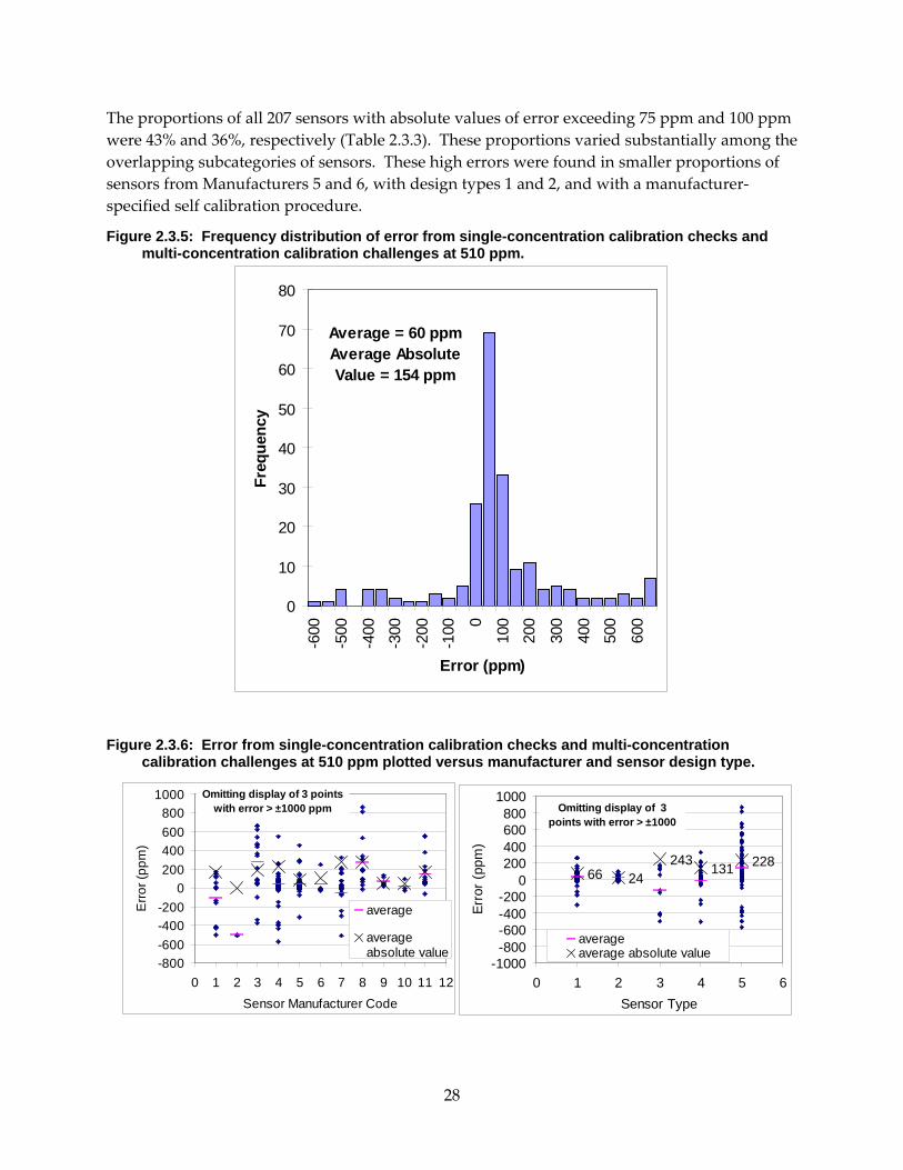
The proportions of all 207 sensors with absolute values of error exceeding 75 ppm and 100 ppm were 43% and 36%, respectively (Table 2.3.3). These proportions varied substantially among the overlapping subcategories of sensors. These high errors were found in smaller proportions of sensors from Manufacturers 5 and 6, with design types 1 and 2, and with a manufacturer-specified self calibration procedure.

Figure 2.3.5: Frequency distribution of error from single-concentration calibration checks and multi-concentration calibration challenges at 510 ppm.

0

10

20

30

40

50

60

70

80-6

00

-500

-400

-300

-200

-100 0

100

200

300

400

500

600

Error (ppm)

Freq

uenc

y

Average = 60 ppmAverage Absolute Value = 154 ppm

Figure 2.3.6: Error from single-concentration calibration checks and multi-concentration calibration challenges at 510 ppm plotted versus manufacturer and sensor design type.

-800-600-400-200

0200400600800

1000

0 1 2 3 4 5 6 7 8 9 10 11 12Sensor Manufacturer Code

Erro

r (pp

m)

average

averageabsolute value

Omitting display of 3 points with error > ±1000 ppm

66 24243 131 228

-1000-800-600-400-200

0200400600800

1000

0 1 2 3 4 5 6Sensor Type

Erro

r (pp

m)

averageaverage absolute value

Omitting display of 3 points with error > ±1000

28

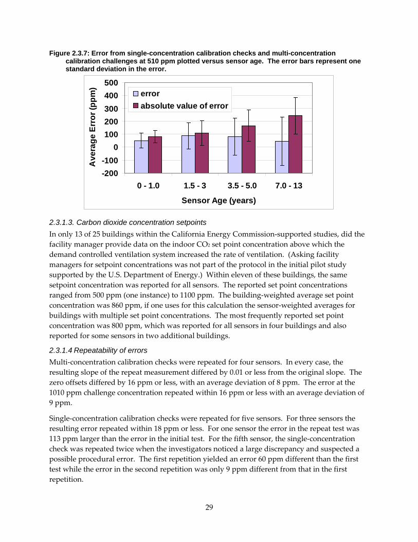
Figure 2.3.7: Error from single-concentration calibration checks and multi-concentration calibration challenges at 510 ppm plotted versus sensor age. The error bars represent one standard deviation in the error.

-200-100

0100200300400500

0 - 1.0 1.5 - 3 3.5 - 5.0 7.0 - 13

Sensor Age (years)

Ave

rage

Err

or (p

pm)

errorabsolute value of error

2.3.1.3. Carbon dioxide concentration setpoints In only 13 of 25 buildings within the California Energy Commission-supported studies, did the facility manager provide data on the indoor CO2 set point concentration above which the demand controlled ventilation system increased the rate of ventilation. (Asking facility managers for setpoint concentrations was not part of the protocol in the initial pilot study supported by the U.S. Department of Energy.) Within eleven of these buildings, the same setpoint concentration was reported for all sensors. The reported set point concentrations ranged from 500 ppm (one instance) to 1100 ppm. The building-weighted average set point concentration was 860 ppm, if one uses for this calculation the sensor-weighted averages for buildings with multiple set point concentrations. The most frequently reported set point concentration was 800 ppm, which was reported for all sensors in four buildings and also reported for some sensors in two additional buildings.

2.3.1.4 Repeatability of errors Multi-concentration calibration checks were repeated for four sensors. In every case, the resulting slope of the repeat measurement differed by 0.01 or less from the original slope. The zero offsets differed by 16 ppm or less, with an average deviation of 8 ppm. The error at the 1010 ppm challenge concentration repeated within 16 ppm or less with an average deviation of 9 ppm.

Single-concentration calibration checks were repeated for five sensors. For three sensors the resulting error repeated within 18 ppm or less. For one sensor the error in the repeat test was 113 ppm larger than the error in the initial test. For the fifth sensor, the single-concentration check was repeated twice when the investigators noticed a large discrepancy and suspected a possible procedural error. The first repetition yielded an error 60 ppm different than the first test while the error in the second repetition was only 9 ppm different from that in the first repetition.

29

2.3.1.5 Errors from energy management systems versus sensor displays Because the main objective of this research was to evaluate sensor accuracy, primary analyses relied on data from sensor displays whenever available. However, for 38 sensors in six buildings, all where multi-concentration calibration checks were performed, data were collected from both the sensor display and the energy management system’s computer display. The errors at the 510, 760, and 1010 ppm challenges of the 38 sensors yielded 113 instances in which errors based on data from energy management systems could be compared to errors based on sensor displays. The average of the absolute value of the difference between the paired estimates of error was 25 ppm; however, excluding data from two sensors located within the same building, the average difference was 10 ppm. For the two sensors in which data from the energy management system and sensor display differed dramatically, the average absolute value difference was 290 ppm. For at least one of these sensors, it was clear that the energy management system’s data was not from the correct sensor. In general; however, these findings indicate that the substantial measurement errors found in this study are sensor errors, not errors in translating the sensor output signals to the energy management systems.

2.3.1.6 Statistical significance of differences in sensor accuracy Table 2.3.4 lists the results of the statistical analyses of sensor errors. The table lists paired categories of sensors for which the average absolute value errors were statistically significantly different, i.e., 95% confidence intervals excluded unity. In bivariate analyses, sensors from Manufacturer 4 (and to a more limited extent from Manufacturer 5) tended to have significantly smaller errors than errors from most of the other manufacturers. Also, sensor type 1 (single lamp single wavelength) tended to have smaller errors than other sensor types except type 4 (single lamp dual wavelength). In some cases, sensors with a reported self-calibration had statistically significantly smaller errors than sensors without a reported self-calibration. In general, error was not significantly associated with sensor age. Many of the differences found to be statistically significant in bivariate analyses remained significant in the multivariate analyses, except self-calibration was no longer a significant predictor of error, presumably because self-calibration is correlated with sensor manufacturer and sensor type which are better predictors of error. The multivariate analyses identified a few statistically significant differences in average errors that were not evident in the bivariate analyses, possibly because the bivariate analysis method is slightly more conservative.

30

Table 2.3.4: Differences in averages of absolute value errors that were statistically significant (p<0.05)*

Analyses Dataset Category Bivariate Multivariate

Multi-Concen-tration

Calibration Challenge, 760 ppm

Manufacturer Sensor Type

Self-Calibration Sensor Age

Error (M4) < Error (M5, M7) Error(T1) < Error(T2)

--- ---

Error(M4) < Error(M7) Error(T1) < Error(T2) Error

(T5) < Error(T2)

--- ---

Multi-Concen-tration

Calibration Challenge, 1010 ppm

Manufacturer

Sensor Type

Self-Calibration

Sensor Age

Error(M4) < Error(M7) Error(M5) < Error(M7)

Error(T1+T2) < Error(T3+T4+T5)

Error(with SC) < Error(without SC) ---

---

---

---

---

Combined

Manufacturer

Sensor Type

Self-Calibration

Sensor Age

Error(M4) < Error(M3, M8) Error(M5) < Error(M3, M7, M8)

Error(M7) < Error(M3)

Error(T1) < Error(T3, T5) Error(T2) < Error(T3, T5)

Error(T4) < Error(T3) Error(T1+T2) < Error(T3+T4+T5)

Error(with SC) < Error(without

SC) Error(Age 0–1 yrs) < Error(Age

5–7 yrs)

Error(M1) < Error(M4) Error(M4) < Error(M3, M7,

M8) Error(M5) < Error(M3, M8)

Error(T1) < Error(T3) Error(T2) < Error(T3) Error(T4) < Error(T3) Error(T5) < Error(T3)

---

Error(Age 3.5–5 yrs) < Error(Age 5–7 yrs)

*Subcategories are indicated by the following symbols: M1 – M8 = manufacturer 1 – manufacturer 8; T1 – T5 = sensor type 1 – sensor type 5, where T1 is single lamp single wavelength, T2 is suspected single lamp single wavelength, T3 is dual lamp single wavelength; T4 is single lamp dual wavelength; T5 = unknown. SC = self calibration

2.3 .2. Evaluation of faulty single-location CO2 sensors Table 2.3.5 provides descriptive information for the faulty single-location CO2 sensors evaluated in the laboratory and the major findings of the evaluations. These faulty sensors are from four manufacturers, have multiple design types, and are two to 13 years old. Four of the nine sensors had either no output signal or had an output signal that changed little or none as the CO2 concentration varied. A fifth sensor repeatedly caused the data acquisition system to shut down, thus, it could not be subjected to tests. Measurements showed that the sensor’s output voltage was highly erratic and the sensor repeatedly attempted to re-initialize its operation. Thus, five of nine sensors were essentially non-functional, although four of these were approximately 13 years old. Sensor FS4 had stable errors which varied with CO2 concentration between 240 to 410 ppm before the manufacturer’s zero and span gas calibration protocol were implemented; subsequently, its errors were 33 to 76 ppm (Figure 2.3.8). Sensor FS5, which had a 310 ppm error in the field setting, had errors of 0 to 95 ppm in the laboratory (after the

31

conditioning period) and these errors did not change significantly after implementing the manufacturer’s calibration protocol which involved only use of a zero-CO2 gas. Sensors FS6 and FS7 had fluctuating errors of five to 158 ppm and 79 to 310 ppm, respectively, during the laboratory studies, which were much smaller than the approximately 800 ppm errors in the field setting for both of these sensors, which came from the same building. The smaller errors observed in the laboratory studies of Sensors FS5 – FS7, relative to the errors observed for the same sensors in the field studies, might be a consequence of automatic calibration corrections during the 11 days of sensor deployment in the laboratory (if CO2 concentrations in the field setting were not regularly decreasing to the outdoor CO2 concentration) and for FS7 the trends suggest further improvements in accuracy (Figure 2.3.9). Another possibility is that there were signal processing problems in the field settings. These sensors had no output displays; therefore, the original field studies of the accuracy of these sensors accuracy relied on the CO2 concentrations reported by energy management systems.

The visual inspection of sensor electronics by an electronics expert indicated no visually obvious electronics failures except in the one sensor with an erratic output voltage that caused the data acquisition system to shut down. In this sensor, an electrical pin that extended out the back of the circuit board and plugged into a socket in the wall mounting plate had a loose pin. This electrical pin became totally disconnected from the circuit board during the inspection process.

The visual inspections of optical cells indicated small amounts of particle deposits or corrosion on the reflective surfaces of the optical cells of six sensors. The amount of deposits or corrosion was never large enough to be a definite source of sensor malfunction. One older non-functional sensor had a window between the optical cell and detector that was partially soiled or discolored. In two sensors, there were one or more small holes, roughly 0.5 mm in diameter, in the fabric covered openings to optical cells. These fabric covered openings provide the path for CO2 to “diffuse” into the cells while excluding airborne particles.

In summary, these evaluations of faulty sensors did not identify definite causes of sensor failures. The study did determine that four of the nine sensors had an output signal that was essentially invariable with CO2 concentration and that a fifth sensor had a highly erratic output signal; i.e., the sensors were non-functional, yet still deployed. The evaluations did identify slight soiling or corrosion of optical cells and, in two sensors, holes in the fabrics through which CO2 diffuses into optical cells which may have contributed to performance degradations. In one of two cases when a manufacturer’s calibration protocol could be implemented, sensor accuracy was clearly improved after the protocol was implemented.

32

Table 2.3.5: Properties of faulty sensors evaluated in the laboratory and key findings.

I.D. Man No.*

Sen-sor

Type#

Self Calibra

-tion

Sen-sor Age (yr)

Man has Cal+ Protocol

Summary of Findings Results of

Inspection of Optical Cell

FS1 1 3 -- ~ 13 Yes*

very small response to changing CO2 concentrations

slight soiling of window between cell and detector

FS2 1 3 -- ~ 13 Yes*

small response to changing CO2 concentrations

no evidence of soiling or corrosion

FS3 4 5^ -- ~ 13 Yes no response to changing

CO2 concentrations

hole in fabric covered opening to

cell; scattered particle deposits

FS4 4 1 yes 5 Yes

large accuracy improvement after

implementing manufacturer’s

recommended calibration protocol

no evidence of soiling or corrosion

FS5 5 1 yes 2 Yes

fair to good accuracy after 11 days; errors fluctuated up to 60 ppm; accuracy

not improved after implementing

manufacturer's calibration

soiling or corrosion of cell near lamp

FS6 8 5# yes 3 No

error initially ~ 500 ppm at ~ 1200 ppm, avg. error ~ 50 ppm at 1000 ppm after 11 days, errors fluctuated

up to 150 ppm

scattered minor pits or soiling of cell

walls

FS7 8 5+ yes 3 No

error initially ~ 500 ppm at ~ 1200 ppm, avg. error ~ 60 ppm at 1000 ppm after 11 days, errors fluctuated

up to 230 ppm

scattered minor pits or soiling of cell

walls

FS8 4 1 yes ~13 Yes no output signal

multiple holes in fabric covered

openings to cell

FS9 4 1 yes 3 Yes

highly erratic output signal caused data acquisition system to shut down,

loose electrical pin (see text), no

evidence of soiling or corrosion

*Man = Manufacturer #Type 1 is single lamp single wavelength, Type 3 is dual lamp single wavelength; Type 5 = unknown type +Cal = Calibration ^single lamp # dual lamp **hardware required for calibration is no longer available

33

Figure 2.3.8: Improvement in accuracy of sensor FS4 after implementing the manufacturer’s recommended calibration protocol.

-100

0

100

200

300

400

500

0 20 40 60 80 100 120

Days of Operation in Laboratory

Err

or (p

pm)

At 473 ppmAt 703 ppmat 1006 ppmAt 1470 ppm

Sensor FS4

Before Implementing Calibration After Calibration

Figure 2.3.9: Improvement in accuracy of sensor FS7 during early period of operation in the laboratory.

0

50

100

150

200

250

300

350

400

0 20 40 60 80 100 120Days of Operation in Laboratory

Err

or (p

pm)

At 473 ppmAt 703 ppmat 1006 ppmAt 1470 ppm

Sensor FS7

2.3.3. Pilot evaluation of CO2 demand controlled ventilation with multi-location sampling systems In Building M1, the challenges with calibration gas mixtures were implemented twice to evaluate three multi-location CO2 measurement systems. Data from the first implementation of the protocol were judged potentially unreliable because the bags of calibration gases may not

34

have been installed on the sample inlet tubes for a sufficient period; thus, these data have not been utilized. The initial data were reviewed with the manufacturer who, prompted by the test results, evaluated the system and identified and fixed some leaks in the sampling system, prior to the second implementation of the multi-concentration calibration protocol. Thus, the data obtained from studies in Building M1 may not be typical of data for this CO2 monitoring system. In addition to employing the multi-concentration calibration protocol, the accuracy of CO2 measurements in Building M1 was also measured using the calibrated reference CO2 instrument which measured CO2 concentrations for approximately 30 minute periods at the same locations of the building’s multi-location CO2 measurement systems. Table 2.3.6 provides the results from these studies. The average and standard deviation of error in indoor CO2 concentration when the systems were challenged with calibration gas mixtures with CO2 concentrations of 525 to 953 ppm was 69 ppm and 40 ppm, respectively. In 13 of 18 cases, the error was less than 25 ppm. For the same concentration range, the average and standard deviation of error in indoor minus outdoor CO2 concentration difference were 14 ppm and 39 ppm, respectively, and in 16 of 18 cases the error was 36 ppm or smaller. Errors were markedly higher at reference CO2 concentrations of 1680 and 1844 ppm, but errors in measurements at such high concentrations, which should not occur in buildings with demand controlled ventilation, are not particularly important. Thus, at the concentrations of interest, the indoor-outdoor CO2 concentration difference, which is the appropriate input to the demand controlled ventilation system, was measured with little error at least at a large majority of the investigated locations.

Figure 2.3.10 shows the results of evaluations of the single multi-location CO2 measurement system in Building M2. The figure compares the concentrations reported by the building’s measurement system to the concentrations measured simultaneously with three co-located calibrated reference CO2 instruments. At all three locations, the building’s measurement system utilized the same CO2 sensor and the measured concentrations were approximately 110 ppm greater than the reference measurements of CO2 concentration. Outdoor CO2 concentrations measured by the building’s measurement system averaged approximately 510 ppm, which is approximately 110 ppm larger than the typical outdoor air CO2 concentration. Because the offset error is approximately the same for the indoor and outdoor CO2 measurements, the error in the difference between indoor and outdoor CO2 concentration within this building is small. Consequently, as in Building M1 the indoor-outdoor CO2 concentration difference, which is the appropriate input to the demand controlled ventilation system, was measured with little error at least at the investigated locations.

In both buildings, the multi-location CO2 monitoring system was installed as part of the process to obtain Leadership in Energy and Environmental Design (LEED certification) and utilized for demand controlled ventilation. Based on a discussion with the facility manager of building M1, the measurement system was one-year old, the CO2 setpoint was 800 ppm above the outdoor CO2 concentration, they experienced no problems with the system, and calibrated sensors were provided every six months via a contract with the manufacturer. From discussions with the facility manager of building M2, the multi-location CO2 measurement system was 10 months old, calibrated replacement sensors were provided four times per year by the manufacturer, and

35

there had been some commissioning difficulties but no subsequent system problems. No information on the CO2 setpoint was provided.

Neither facility manager directly provided information on initial system costs, however, the manufacturer estimated that installed costs were typically $1500 to $2500 per sensed location. The system from this manufacturer includes special sampling components that are needed for pollutants other than CO2, thus, it is not cost optimized for CO2 – only measurements. The manufacturer’s reported cost of calibration services (providing calibrated replacement sensors every six months and replacing sensors when needed), real time sensor diagnostics, warranty, and data services, and was estimated to be $60 to $125 per year per sensed location. For comparison, the cost of traditional demand controlled ventilation with single-location CO2 sensors used for development of the Title 24 standard is $617 per sensor after adjustment for inflation (Hong and Fisk 2009). However, a $1540 per sensor cost can be derived from a cost analysis of obtaining LEED certification (Steven Winters Associates 2004).

36

Table 2.3.6: Results of evaluations of multi-location CO2 measurement systems in Building M1.

System Location Reference CO2 Concentration

(ppm)

Error in Indoor CO2

Concentration (ppm)

Error in Indoor Minus Outdoor

CO2 Concentration

Difference (ppm)

-----------------------Challenges with calibration gasses------------------------ 1 1125 525 80 25 1 3126 525 27 -21 1 3135 525 38 -18 3 1230 569 34 -18 3 2202 569 40 -13 3 2204 569 39 -19 2 4126 570 44 -14 2 5126 570 100 36 2 5163 570 47 -11 3 1230 861 54 -3 3 2202 861 73 22 3 2204 861 64 11 2 4126 867 72 10 2 5126 867 155 98 2 5163 867 78 19 1 1125 953 174 118 1 3126 953 55 0 1 3135 953 73 25 1 1125 1,680 323 276 1 3126 1,680 124 66 1 3135 1,680 131 75 2 4126 1,844 193 133 2 5126 1,844 363 304 2 5163 1,844 200 135

Average and (Standard Deviation) of all results with CO2 < 1000 ppm 69 (40) 14 (39)

---Evaluation with co-located reference CO2 instrument----- 1 2116 427 12 -36 2 5163 543 54 0 2 5163 676 67 11 3 1122 429 31 -24 3 1230 478 36 -23

37

Figure 2.3.10: Results of evaluations of the multi-location CO2 measurement system in building M2.

2.3.4. Spatial variability of CO2 concentration in meeting rooms Figure 2.3.11 provides an example plot of the results of multipoint monitoring of carbon dioxide concentrations during a noon-time seminar in a crowded 76 m2 conference room. In this instance, the CO2 concentrations, varied among locations at any one time by up to approximately 300 ppm, and fluctuated substantially with time at many locations. Concentrations at return grilles were in the middle of the range. The concentration at the west wall location may be lowest because the people were not located close to this location which was directly below the screen used for display of presentations. Concentrations measured at the 0.3 m height on the east wall are moderately lower than concentrations measured at the 1.4 and 1.8 m heights.

In three of six meeting rooms, concentrations fluctuated rapidly as illustrated in Figure 2.3.11, potentially, in part, because of the CO2 in exhaled breath from people near sample points. During measurements in meeting rooms 1 and 4, it is known that the rooms were very crowded with people sitting or standing near sample locations. The CO2 concentrations measured by the sensors used for demand controlled ventilation applications will most likely vary less, as these sensors sample diffusively and respond more slowly than the instruments used in this research. In the remaining three meeting rooms, concentration fluctuations, as illustrated in Figure 2.3.12, were less pronounced.

Data similar to those illustrated in Figures 2.3.11 and 2.3.12 were collected from seven total time periods in six meeting rooms. Table 2.3.7 provides information on the meeting rooms and measured CO2 concentrations. From each data set, period-average (i.e., time-average over the selected time period) CO2 concentrations are provided at each measurement location for periods of 30 to 90 minutes when concentrations were elevated above background due to occupancy of the meeting room. For the example datasets shown in Figure 2.3.11 and 2.3.12, concentrations were averaged for the 12:15 to 13:00 and 14:10 to 14:55 time periods, respectively. The range in period-average CO2 concentrations at the wall mounted sample points located in the same

Multi-location System, Building M2, Room 207

300

400

500

600

700

800

900

1,000

12:00 13:00 14:00 15:00 16:00 17:00 18:00

CO

2 Con

cent

ratio

n (p

pm) Measured, Room 207

Reference

Measured- 110 ppm,Room 207

38

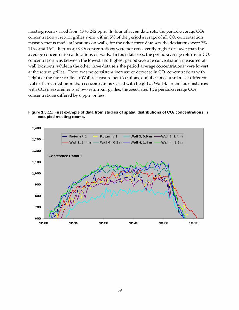
meeting room varied from 43 to 242 ppm. In four of seven data sets, the period-average CO2 concentration at return grilles were within 5% of the period average of all CO2 concentration measurements made at locations on walls, for the other three data sets the deviations were 7%, 11%, and 16%. Return-air CO2 concentrations were not consistently higher or lower than the average concentration at locations on walls. In four data sets, the period-average return-air CO2 concentration was between the lowest and highest period-average concentration measured at wall locations, while in the other three data sets the period average concentrations were lowest at the return grilles. There was no consistent increase or decrease in CO2 concentrations with height at the three co-linear Wall-4 measurement locations, and the concentrations at different walls often varied more than concentrations varied with height at Wall 4. In the four instances with CO2 measurements at two return-air grilles, the associated two period-average CO2 concentrations differed by 6 ppm or less.

Figure 1.3.11: First example of data from studies of spatial distributions of CO2 concentrations in occupied meeting rooms.

600

700

800

900

1,000

1,100

1,200

1,300

1,400

12:00 12:15 12:30 12:45 13:00 13:15

Return # 1 Return # 2 Wall 3, 0.9 m Wall 1, 1.4 m

Wall 2, 1.4 m Wall 4, 0.3 m Wall 4, 1.4 m Wall 4, 1.8 m

Conference Room 1

39

Figure 2.2.12: Second example of data from studies of spatial distributions of CO2 concentrations in occupied meeting rooms.

Table 2.3.7: Spatial variability of CO2 concentrations in occupied meeting rooms. The numbers are averages and standard deviations for 30 – 90 minute meetings, unless indicated otherwise.

Conf, Room 1 2 3 3 4 5 6 Floor Area (m2) 76 45 59 59 160 115 46 Ceiling Height (m) 2.7 2.7 2.8 2.8 2.7 – 4.7 3.0 3.0

CO2 Concentration (standard deviation) in ppm or Concentration Ratio Wall 1 902 (48) 722 (23) 675 (5) 626 (23) 1,668 (185) 943 (145) 640 (68) Wall 2 960 (51) 724 (32) 648 (8) 599 (16) 1,774 (166) 909 (160) 515 (43) Wall 3 811 (45) 719 (34) 632 (7) 594 (17) 1,910 (263) 964 (137) 562 (58) Wall 4 Low 1007 (39) 708 (22) 635 (7) 582 (19) 1,672 (238) 903 (100) 533 (49) Wall 4 medium 1029 (51) 704 (36) 635 (6) 583 (18) 1,734 (232 961 (153) 554 (61) Wall 4 high 1042 (53) 651 (64) 634 (6) 584 (18) 1,759 (243) 945 (126) 571 (80) Wall 5 NA NA NA NA 1,823 (277) 967 (177) 621 (74) All Wall locations 959 (94) 704 (47) 643 (17) 595 (23) 1,754 (247) 940 (146) 571 (75) All Wall (max – min)* 231 73 43 43 242 64 124

Return Grille 1 931 (43) 593 (30) 669 (5) 616 (16) NA NA NA Return Grille 2 925 (54) 596 (34) 668 (5) 615 (17) 1,877 (216) 890 (124) 510 (48) Return Average / All Wall Average 0.97 0.84 1.04 1.03 1.07 0.95 0.89

Supply 433 (6) 451 (18) 613 (5) 581 (14) 1,413 (150) 849 (130) 424 (5) *maximum minus minimum of average CO2 concentrations measured at locations on walls

^return grille was mounted in a wall, not in the ceiling of the meeting room

500

550

600

650

700

14:00 14:10 14:20 14:30 14:40 14:50 15:00 15:10

Wall 1, 1.5 m Return # 2 Return # 1Wall 2, 1.5 m Wall 3, 1.55 m Wall 4, 0.46 mWall 4, 1.2 m Wall 4, 1.7 m

Conference Room 3

40

2.4 Discussion

2.4.1 Accuracy requirements To place the results of this study in context, one must have an estimate of the required accuracy of CO2 sensors used in commercial buildings for demand controlled ventilation. While most systems only measure the indoor CO2 concentration, the difference between indoor and outdoor CO2 concentration is a better indicator of building ventilation rate, and outdoor CO2 concentrations in urban areas can vary significantly with location and time. One needs to be able to determine with reasonable accuracy the difference between peak indoor and outdoor CO2 concentrations found in commercial buildings. The most representative data set is that obtained from a survey of 100 office buildings by the U.S. Environmental Protection Agency (EPA). This EPA study measured and recorded five-minute-average CO2 concentrations at three indoor locations and one outdoor location. If one considers the maximum one-hour average differences between indoor and outdoor CO2 concentration3 from this EPA study, the minimum was 55 ppm, maximum was 777 ppm, average was 310 ppm, and median was 269 ppm. If one desires no more than a 20% error in measurements of the average peak indoor-outdoor CO2 concentration difference, then 62 ppm (one fifth of 310 ppm) is a minimum expectation for CO2 measurement accuracy in offices. The California Title 24 Standard requires a similar level of accuracy “the CO2 sensors must be factory certified to have an accuracy of no less than 75 ppm over a five year period without recalibration in the field”. Seventy five parts per million corresponds to 16% of the difference between the average set point concentration (860 ppm) reported in this study and the typical outdoor carbon dioxide concentration of 400 ppm.

2.4.2 Accuracy of single-location CO2 sensors This study employed two protocols to evaluate sensor error – multi-concentration calibration checks and single-concentration checks. The data from the multi-concentration calibrations, performed whenever possible, have the greatest value because these data yield estimates of sensor accuracy at typical CO2 setpoint concentrations. The errors at 760 and 1010 ppm may be the most useful indicators of sensor accuracy. The slope and zero offset errors can be counteracting; thus, neither provides a clear indication of overall sensor performance. There is a general consistency among the findings obtained via the two evaluation protocols. The results of both protocols indicate that many sensors had large errors. In general, both protocols indicate that the same subgroups of sensors had superior (or inferior) average performance.

The findings of this research indicate that a substantial fraction of CO2 sensors had errors greater than specified in Title 24 or provided in the applicable product specifications. Forty seven percent of sensors had errors greater than 75 ppm at a concentration of 760 ppm and 40% of sensors had errors greater than 75 ppm at a concentration of 1010 ppm. A significant fraction of sensors have much larger errors, e.g., > 300 ppm. These concentrations of 760 and 1010 ppm are typical of the setpoint concentrations at which demand controlled ventilation systems

3 Based on the first authors’ analyses of the CO2 data from this study.

41

increase outdoor air ventilation rates. Thus, overall many CO2 sensors do not meet accuracy requirements

Sensors from specific manufacturers, with a single lamp single wavelength design, and with a self-calibration procedure specified in product literature, had better average accuracy. After multivariate statistical analyses of the data, sensors from some manufacturers had a better average accuracy (particularly Manufacturer 4) and Type 1 sensors (with a single lamp single wavelength design) were generally associated with statistically significantly higher average accuracy. However, use of sensors only in these categories, while helpful, would not result in widespread compliance with the Title 24 accuracy requirements. Twenty one and 37% of sensors from Manufacturer 4 and 20% and 27% of Type 1 sensors still had errors greater than 75 ppm at 760 ppm and 1010 ppm, respectively.

In general, all or most of the sensors within each building were the same model and had the same or a similar age. Thus, sensor manufacturer and sensor type are correlated with the building identification code. In theory, differences in maintenance and calibration practices among buildings might partially explain the observed associations of accuracy with sensor manufacturer and features. However, given that none of the facility managers reported that they had calibrated the sensors in their buildings subsequent to the initial sensor installation, the manufacturer and the sensor design are more likely the real explanation for the observed variability in sensor accuracy.

A significant number of sensors in all age sensor categories had large errors. Thus, replacing sensors every few years also would not solve the accuracy problem.

Because the results obtained from energy management systems generally agreed well with results obtained from sensor displays, the measurement errors appear to be primarily a consequence of sensor problems and not a consequence of errors in translating the sensor output signals to building energy management systems. Having a display on the sensor may, however, be advantageous as it facilitates checks of sensor assignment in the energy management software. Also, periodic visual checks of sensor displays could help facility managers identify obviously faulty sensors.

The analyses of a sample of nine faulty sensors failed to identify definite causes of sensor failures. The fact that four of the nine sensors had an output signal that was essentially invariant with CO2 concentration, yet these sensors were still deployed, indicates that facility managers are not always aware of obviously faulty sensors. These findings suggest that sensor fault detection systems that provide alarms when sensors are clearly faulty (e.g., have invariable outputs) may be beneficial for maintaining performance of demand controlled ventilation systems.

Three of the faulty sensors were 13 years old, the highest sensor age encountered in the study. One might conclude that 13 year old sensors would be expected to be faulty and should have been replaced, although the manufacturer’s product literature does not specify a sensor lifetime. However, if we exclude the data from one outlier with an error of 1486 ppm, the average error of all the 13 year old sensors in the study was the same as the average error of the seven year

42

old sensors. Also, the average error of 7 to 13 year old sensors was not statistically significantly higher than the average age of 3.5 to 5 year old sensors. Thus, the study data provide no clear indication of how long sensors should be deployed.

The Iowa Energy Center (National Buildings Controls Information Program 2009) provides the results from a laboratory-based study of the accuracy of 15 models of new single-location CO2 sensors. Although their report does not provide summary statistics, their findings are broadly consistent with the findings of the field studies of CO2 sensor accuracy described in this report. Many of the new CO2 sensors had errors greater than 75 ppm, and errors greater than 200 ppm were not unusual. Maximum errors of new sensors approached 500 ppm.

It is important to keep in mind that the reference CO2 measurements used in this study to evaluate sensor accuracy are imperfect. The linearity of the reference CO2 instrument, cross comparisons with other instruments, and checks of performance using multiple calibration gases instill confidence in the reference measurements; however, errors of a few percent are still likely. If these errors were systematic, the reported average errors of CO2 sensors installed in buildings and reported fractions of sensors with large errors could change significantly; however, the main findings and conclusions of this research are not likely to be substantially impacted by errors in the reference CO2 measurements.

2.4.3 Accuracy multi-location CO2 monitoring systems The data from the pilot studies of the accuracy of multi-location CO2 monitoring systems are insufficient as a basis for any firm conclusions about the accuracy of these systems; however, the limited results obtained were encouraging. The study results illustrate the advantage of incorporating a measurement of outdoor air CO2 concentration with each sensor – offset errors cancel out in the indoor minus outdoor CO2 concentration difference. For widespread acceptance, it seems likely that the costs of these systems will need to be reduced.

2.4.4 Spatial variability of CO2 concentration in meeting rooms The purpose of the multipoint measurements of CO2 concentrations in occupied meeting rooms was to provide information for locating the CO2 sensors in meeting rooms. The Title 24 standard requires that CO2 be measured between 0.9 and 1.8 m (3 and 6 ft) above the floor with no less than one sensor per 930 m2 of floor area. The results of the multipoint measurements varied among the meeting rooms. In some instances, concentrations at different wall-mounted sample points varied by more than 200 ppm and concentrations at these locations sometimes fluctuated rapidly. These concentration differences may be a consequence, in part, of the high concentrations of CO2 (e.g., 50,000 ppm) in the exhaled breath of nearby occupants. Because the results of the multipoint measurements varied among meeting rooms, this research does not result in definitive guidance for locating sensors in meeting rooms; however, the results suggest that measurements at return-air grilles may be preferred to measurements at wall-mounted locations. In four out of seven data sets, CO2 concentration at return-grille locations fell between the maximum and minimum of CO2 concentrations at wall-mounted locations and in five of seven data sets, the period average concentration at return grilles was within 10% of the period average concentration measured from sample points on walls.

43

2.4.5 Overall findings and their implications Together, the findings from the laboratory studies of the Iowa Energy Center and current field studies indicate that many CO2 based demand controlled ventilation systems will fail to meet the design goals of saving energy while assuring that ventilation rates meet code requirements. Given this situation, one must question whether the current prescriptions for demand controlled ventilation in the Title 24 standard are appropriate. However, given the importance of ventilation, and considering the energy savings potential of demand controlled ventilation, technology improvement activities by industry and further research, are warranted. Some possible technical options for improving the performance of demand controlled ventilation are listed below:

• Manufacturers of single-location CO2 sensors for demand controlled ventilation applications make technology changes that improve CO2 sensor accuracy. Sensor costs are likely to increase.

• Users of CO2 sensors for demand controlled ventilation applications perform sensor calibrations immediately after initial sensor installation and periodically thereafter. Research is needed to determine if such a protocol would maintain accuracy and whether costs would be acceptable. At present, such calibrations appear to be very rare as facility managers are continuously facing other demands.

• Demand controlled ventilation systems use existing CO2 sensors that are more accurate, stable, and expensive than the sensors traditionally used for demand controlled ventilation. To spread the cost of these sensors, multi-location sampling systems may be necessary. Pilot scale evaluations of this option included in this project are too limited for conclusions but suggest that these systems may be more accurate. Costs will likely need to be reduced.

• Demand controlled ventilation systems may be controlled by systems that count occupants, as opposed to by systems that measure CO2 concentrations. Two optical systems for counting occupants as they pass through doorways were evaluated and the findings are provided in Chapter 4. Other people-counting options may be feasible, such as radio frequency identification that is now used routinely to indicate location of inventories are provide occupants access through normally locked building doors. With further development, people counting systems might be an attractive alternative to CO2 sensors for demand controlled ventilation.

It is clear that further research will be necessary to develop and evaluate these technical options. Policy changes, such as changes in aspects of the Title 24 standard pertaining to demand controlled ventilation, may be an option for stimulating the necessary technology development. Chapter 5 provides recommendations related to prescriptions for demand controlled ventilation in Title 24.

44

2.6. Conclusions

The accuracy of single-location CO2 sensors, as they are applied and maintained for demand controlled ventilation in commercial buildings, is frequently less than specified in the Title 24 standard and frequently less than needed to meet the design goals of saving energy while assuring that ventilation rates meet code requirements.

The average accuracy of single-location CO2 sensors varies among manufacturers and is higher with a single lamp single wavelength design. However, use of sensors only from the manufacturer with the best average accuracy or only single lamp single wavelength sensors, while helpful, would not result in widespread compliance with the Title 24 sensor accuracy requirements.

Accuracy varied substantially in each age category and, in general, the association of sensor age with accuracy was not statistically significant. Replacing CO2 sensors every few years would not result in widespread compliance with the Title 24 sensor accuracy requirements.

Because the results obtained from energy management systems generally agreed well with results obtained from sensor displays, the measurement errors of single-location CO2 sensors appear to be primarily a consequence of sensor problems and not a consequence of errors in translating the sensor output signals to building energy management systems.

No facility manager indicated that they had calibrated the single-location CO2 sensors in their facility, after the initial sensor installation and checkout period.

The data from the pilot studies of the accuracy of multi-location monitoring systems are insufficient as a basis for firm conclusions about the accuracy of these systems; however, the limited results obtained were encouraging. For widespread acceptance, it seems likely that system costs will need to be reduced.

Because the results of the multipoint CO2 concentration measurements varied among meeting rooms, this research does not result in definitive guidance for locating sensors in meeting rooms; however, the results suggest that measurements at return-air grilles may be preferred to measurements at wall-mounted locations.

Changes are needed in technologies used for demand controlled ventilation. Research and policy changes may be necessary to stimulate the needed technology improvements.

45

CHAPTER 3: Assessment of Energy Savings Potential from Use of Demand Controlled Ventilation in General Office Spaces in California

3.1. Background

Most building codes require that a minimum amount of outdoor air be provided to ensure adequate IAQ. To comply, ventilation systems typically are designed to operate with a fixed minimum outdoor air supply rate usually based on design occupancy that is much higher than occupancy levels during most of the time. While measured data on the minimum ventilation rates in existing offices are limited and subject to large measurement error, a survey of 100 U.S. office buildings supported by the U.S. Environmental Protection Agency provides the best available data (Persily and Gorfain 2008). The measurements of ventilation rates in this survey collected when HVAC systems should be supplying minimum amounts of outdoor air were analyzed by the first-named author of this report and indicate that, on average, minimum ventilation rates dramatically exceed code requirements that are typically 7.1 to 9.4 L/s per occupant depending on occupant density (California Energy Commission 2008). The high measured ventilation rates are partly a consequence of the low average occupant density in offices, relative to the design density, but may also be due to the absence, in most office buildings, of any real-time measurement and feed-back-control system for minimum ventilation rates.

To address the problems of too much or too little outdoor air, the HVAC system can use a demand controlled ventilation strategy to tailor the amount of outdoor air to the occupancy level. CO2 sensors have emerged as the primary technology for indirectly monitoring occupancy and implementing demand controlled ventilation: CO2 sensors monitor CO2 levels in the indoor air, and the HVAC system uses data from the sensors to adjust the amount of incoming outdoor air. If the HVAC system has an outdoor air economizer, the ventilation rate will be higher than indicated by the demand controlled ventilation controlled system when weather is mild.

Under the 2008 California Building Energy Efficiency Standards (Title 24) (California Energy Commission 2008), demand controlled ventilation is required for a space served by either a single zone system or a multi-zone system with DDC to the zone level that has an air-side economizer if the design occupant density is greater than or equal to 26.9 people per 100 m2, with some exceptions. General office spaces are not subject to the Title 24-2008 demand controlled ventilation requirement; however, given the evidence described above that minimum ventilation rates in offices without demand controlled ventilation are, on average, much higher than required in codes, a significant energy savings from demand controlled ventilation was

46

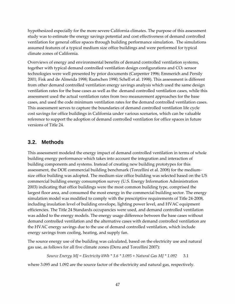
hypothesized especially for the more severe California climates. The purpose of this assessment study was to estimate the energy savings potential and cost effectiveness of demand controlled ventilation for general office spaces through building performance simulation. The simulations assumed features of a typical medium size office buildings and were performed for typical climate zones of California.

Overviews of energy and environmental benefits of demand controlled ventilation systems, together with typical demand controlled ventilation design configurations and CO2 sensor technologies were well presented by prior documents (Carpenter 1996; Emmerich and Persily 2001; Fisk and de Almeida 1998; Raatschen 1990; Schell et al. 1998). This assessment is different from other demand controlled ventilation energy savings analysis which used the same design ventilation rates for the base cases as well as the demand controlled ventilation cases, while this assessment used the actual ventilation rates from two measurement approaches for the base cases, and used the code minimum ventilation rates for the demand controlled ventilation cases. This assessment serves to capture the boundaries of demand controlled ventilation life cycle cost savings for office buildings in California under various scenarios, which can be valuable reference to support the adoption of demand controlled ventilation for office spaces in future versions of Title 24.

3.2. Methods

This assessment modeled the energy impact of demand controlled ventilation in terms of whole building energy performance which takes into account the integration and interaction of building components and systems. Instead of creating new building prototypes for this assessment, the DOE commercial building benchmark (Torcellini et al. 2008) for the medium-size office building was adopted. The medium-size office building was selected based on the US commercial building energy consumption survey (U.S. Energy Information Administration 2003) indicating that office buildings were the most common building type, comprised the largest floor area, and consumed the most energy in the commercial building sector. The energy simulation model was modified to comply with the prescriptive requirements of Title 24-2008, including insulation level of building envelope, lighting power level, and HVAC equipment efficiencies. The Title 24 Standards occupancies were used, and demand controlled ventilation was added to the energy models. The energy usage difference between the base cases without demand controlled ventilation and the alternative cases with demand controlled ventilation are the HVAC energy savings due to the use of demand controlled ventilation, which include energy savings from cooling, heating, and supply fan.

The source energy use of the building was calculated, based on the electricity use and natural gas use, as follows for all five climate zones (Deru and Torcellini 2007):

Source Energy MJ = Electricity kWh * 3.6 * 3.095 + Natural Gas MJ * 1.092 3.1

where 3.095 and 1.092 are the source factor of the electricity and natural gas, respectively.

47

3.2.1. The medium size office building The medium size office building has a rectangular shape about 50 m x 33 m (Figure 3.2.1). It has three identical stories with a total floor area of 4982 m2. Each floor has five thermal zones: four perimeter ones and one core. All five zones are assumed to be general office occupancy. The window-wall-ratio is 33%. The building does not have daylighting controls. The building is served by three packaged variable air volume systems with gas furnace for heating. One system serves one floor. Each of the three packaged variable air volume systems has an air-side economizer which provides up to 100% of outdoor air for free cooling when indoor and outdoor conditions favor economizer operation.

Figure 3.2.1: Three dimensional view the office building with typical floor plan

The building size, shape, and operating schedules stay the same for all locations, but the building efficiency level varies with climate zone according to Title 24-2008 prescriptive requirements. Table 3.2.1 summarizes the internal loads and minimum ventilation rate for the office building based on the Title 24 Standards.

Table 3.2.1: Internal loads and minimum ventilation rate of office buildings

Occupan-cy Type

Design #people per 100

m²

Sensible Heat

W/person

Latent Heat

W/person

Recepta-cle Load

W/m²

Hot Water Load

W/person

Light-ing

Power W/m²

Ventilation L/s/m²

Office Buildings 10.8 73 60 14.4 31 9.15 0.76

48

Figure 3.2.2 shows the occupant schedules for weekdays and weekends with the percentage values representing the number of occupants in the building divided by the design number of occupants, converted to a percentage. These daily profiles are applicable year round, i.e., assuming no seasonal variations.

Figure 3.2.2: Occupancy schedule of office building

0

10

20

30

40

50

60

70

1 2 3 4 5 6 7 8 9 10 11 12 13 14 15 16 17 18 19 20 21 22 23 24

% D

esig

n O

ccup

ancy

Hour

Weekdays

Saturday

Sunday

Five cities representing typical climate regions of California were chosen and are identified in Table 3.2.2. The Title 24 Standards weather data for the chosen five climate zones was used in the simulations.

Table 3.2.2: Five typical California climate zones

Description California Climate Zone Representative City North Coast 3 San Francisco South Coast 6 Los Angeles Central Valley 12 Sacramento Desert 14 China Lake Mountains 16 Mt. Shasta

3.2.2. Outdoor air ventilation rates For the base cases without demand controlled ventilation, a constant outdoor air flow of either 13.2 or 38.2 L/s per occupant was used based on average weekday occupancy when the building is occupied and ventilated. These two values of ventilation rates are based on the

49

measured results from a survey of 100 representative U.S. office buildings and unpublished analyses by the co-author of this report. The survey is the only known U.S. study of ventilation rates and other indoor air quality conditions in a large representative sample of office buildings. Ventilation and HVAC airflow data from this survey are described by Persily and Gorfain (Persily and Gorfain 2008). The survey took place for a broad range of weather conditions and the first-named author of this report analyzed data collected when the outdoor air temperature was above 22°C and, consequently, outdoor air supply rates should be at the minimum given the usual economizer control strategy. The resulting 13.2 L/s/person average minimum ventilation rate is based on analyses of peak measured one-hour average carbon dioxide concentrations, assuming that occupants emit 0.0052 L/s of CO2 and that the measured one-hour peak concentration is 80% of the true equilibrium CO2 concentration. The 38.2 L/s per occupant average minimum ventilation rate is based on use of air velocity sensors to measure outdoor air flow rate, or from the difference between supply and recirculation air flow, both measured using velocity sensors. The two resulting average minimum ventilation rates are very different and, at present, it is not known which value is more accurate.

For the alternative cases with demand controlled ventilation, the space minimum outdoor air flow was calculated, consistent with the Title 24 Standards, as the larger of:

• 8.3 L/s/person times the current number of occupants present, where the current number of occupants equals the design occupancy multiplied by the occupant schedule percentage shown in Figure 3.2.2: Occupancy schedule of office building

• The value of 8.3 L/s per person corresponds to the ventilation rate necessary to maintain indoor carbon dioxide in an office building less than 600 ppm greater than the outdoor concentration assuming a carbon dioxide generation rate per occupant of 0.0052 L/s. This 600 ppm maximum difference between indoor and outdoor concentration is specified for demand controlled ventilation in Title 24-2008.

and

• 0.76 L/s/m² times the space floor area.

An average occupancy that is 50% of design occupancy was selected for the simulations to match typical practice in office buildings (Figure 3.2.2: Occupancy schedule of office building

The 50% average weekday occupancy was used together with the two base case ventilation rates (13.2 or 38.2 L/s per occupant) to set the constant minimum ventilation air flow for the base case simulations. For the demand controlled ventilation cases, the CO2 demand controlled ventilation system increased outdoor air ventilation rates when occupancy is at a higher level. The energy savings potential of demand controlled ventilation is a consequence of its ability to match the rate of outdoor air ventilation with actual occupancy, which is often less than peak design occupancy. With a design occupant density of 10.8 people/100 m² for office buildings,

50

the design outdoor air flow based on the per person requirement is the larger of 0.76 L/s/m² and a time varying rate that is always less than or equal to 0.89 L/s/m2 (8.3 L/s/person X 10.8 people/100 m²). Two alternate design occupancy levels representing a 50% and a 100% higher occupancy are included in the analysis. Table summarizes the minimum outdoor air supply rates for all cases.

For both the base cases and the demand controlled ventilation cases, the packaged variable air volume systems have air side economizers as required by the Title 24 Standards. Therefore, the actual outdoor air flow can exceed the minimum ventilation rate when economizers operate.

Table 3.2.3: Minimum outdoor air requirement

Case Description

Design Occupant Density #people per 100

m²

Weekday Average

Occupant Density # people per 100

m2

Design OA L/s/m²

based on 13.2 L/s/p in base cases or 8.3 L/s/p

in DCV cases

Design OA L/s/m2

based on 38.2 L/s/p in base cases or 8.3 L/s/p

in DCV cases

Title 24 Required Minimum OA L/s/m²

Actual OA Supply L/s/m2

Base Cases

10.8 5.4 0.71 2.03 NA 0.71 or 2.03 16.1 8.0 1.07 3.10 NA 1.07 or 3.10 21.5 10.8 1.42 4.11 NA 1.42 or 4.11

DCV* Cases

10.8 5.4 0.89 (weekday

avg. = 0.088)

0.89 (weekday

avg. = 0.088)

0.76 Varies with time (0.76 to 0.89)

16.1 8.0 1.34 (weekday

avg. = 0.132)

1.34 (weekday

avg. = 0.132)

0.76 varies with time (0.76 to 1.34)

21.5 10.8 1.79 (weekday

avg. = 0.176)

1.79 (weekday

avg. = 0.176)

0.76 varies with time (0.76 to 1.79)

*DCV = demand controlled ventilation

3.2.3. Simulation tool EnergyPlus version 3.0, released in November 2008, was used to simulate the whole building energy performance of the selected medium size office building. The demand controlled ventilation algorithm implemented in EnergyPlus 3.0 is based on the calculation of space minimum outdoor air requirements for varying number of occupants and a constant component based on space floor area. EnergyPlus 3.0 calculates the system-level outdoor air requirement as the sum of space outdoor air flows, without considering zone air distribution effectiveness or system ventilation efficiency as required by ASHRAE standard 62.1-2007 (ASHRAE 2007). This works fine for single zone systems or multi zone systems serving zones with same design occupancy and schedule. In this assessment, all spaces are assumed to be general offices with same design occupancy and schedule.

51

3.2.4. Cost estimates In the demand controlled ventilation measure analysis (Taylor Engineering 2002) for the development of Title 24-2005, the demand controlled ventilation cost for a single zone system was estimated to be $575 which included parts and labor. Adjusted for inflation and multiple zones served by a packaged variable air volume system, the demand controlled ventilation cost for each of the three PVAV systems were estimated to be $3085 (average $617 per zone X 5 zones). On the per building conditioned floor area basis, the demand controlled ventilation cost is $1.86/m2.

Based on a 15 year life cycle and 3% discount rate for an installed demand controlled ventilation system, the present value (PV) of energy costs were estimated to be $1.37/kWh for electricity and $0.069/MJ for natural gas in California (Eley Associates and New Building Institute 2002). These present values cost numbers were multiplied by the changes in annual energy consumption in the estimation of the present value of cost savings for the 15-year life cycle.

3.3. Results

Table 3.3.1 summarizes the simulation results and calculated energy usage and costs savings. The Design OA column lists the equivalent outdoor air rate per floor area converted from the outdoor air rate per occupant. The next three columns show the whole building annual energy use per conditioned floor area. The remaining columns indicate the energy and cost savings for demand controlled ventilation relative to the base cases.

52

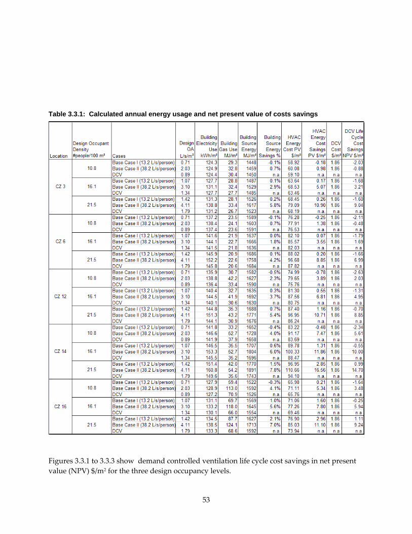
Table 3.3.1: Calculated annual energy usage and net present value of costs savings

Figures 3.3.1 to 3.3.3 show demand controlled ventilation life cycle cost savings in net present value (NPV) $/m2 for the three design occupancy levels.

53

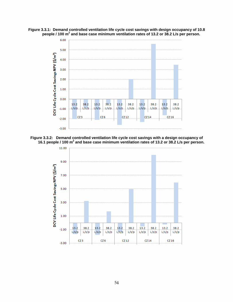
Figure 3.3.1: Demand controlled ventilation life cycle cost savings with design occupancy of 10.8 people / 100 m2 and base case minimum ventilation rates of 13.2 or 38.2 L/s per person.

Figure 3.3.2: Demand controlled ventilation life cycle cost savings with a design occupancy of

16.1 people / 100 m2 and base case minimum ventilation rates of 13.2 or 38.2 L/s per person.

54

Figure 3.3.3: Demand controlled ventilation life cycle cost savings with a design occupancy of 21.5 people / 100 m2 and base case minimum ventilation rates of 13.2 or 38.2 L/s per person.

From Figures 3.3.1 to 3.3.3, it can be seen that with the reference outdoor ventilation rate of 13.2 L/s/person, only for climate zones 14 and 16 do the calculations indicate a marginal life cycle cost savings for demand controlled ventilation when the design occupancy is at 21.5 people per 100 m2. This is probably due to the fact that the demand controlled ventilation cases have higher design ventilation rates than the cases without demand controlled ventilation at a fixed ventilation rate of 13.2 L/s/person for all three occupant density levels. For the base case with a reference ventilation rate of 38.2 L/s/person, the without- demand controlled ventilation cases always have higher ventilation rates than the demand controlled ventilation cases for all three occupant density levels.

Figure 3.3.1 at design occupancy of 10.8 people per 100 m2, demand controlled ventilation is cost effective (positive NPV savings) with the reference outdoor ventilation rate of 38.2 L/s/person for climate zones 12, 14, and 16. The largest estimated savings is $5.62/m2 in climate zone 14, followed by $3.49/m2 in climate zone 16, and $2.03/m2 in climate zone 12.

From Figure 3.3.2 at design occupancy of 16.1 people per 100 m2, demand controlled ventilation is cost effective with the reference outdoor ventilation rate of 38.2 L/s/person in all five climate zones, with the largest savings of NPV $10.0/m2 in climate zone 14, followed by $5.94/m2 in climate zone 16, $4.95/m2 in climate zone 12, $3.22/m2 in climate zone 3, and $1.69/m2 in climate zone 6. The savings are much higher than those at design occupancy of 10.8 people per 100 m2.

From Figure 3.3.3 at design occupancy of 21.5 people per 100 m2, demand controlled ventilation is cost effective with the reference outdoor ventilation rate of 13.2 L/s/person in climate zones 3,

55

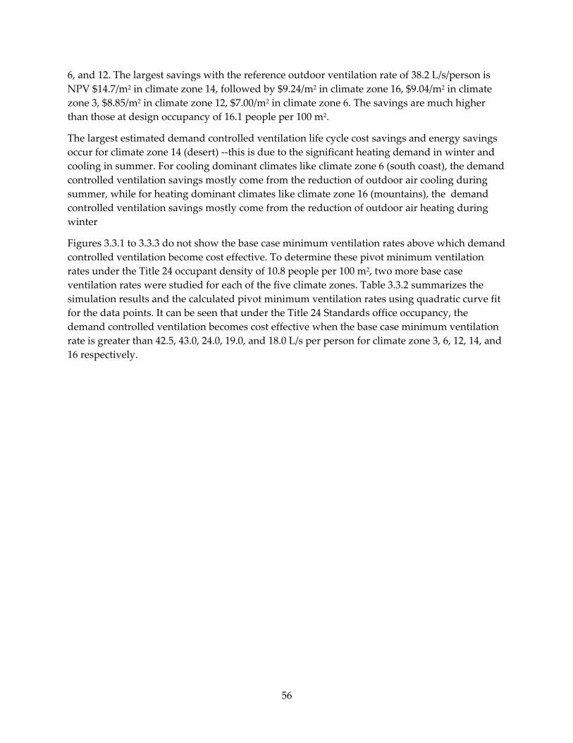
6, and 12. The largest savings with the reference outdoor ventilation rate of 38.2 L/s/person is NPV $14.7/m2 in climate zone 14, followed by $9.24/m2 in climate zone 16, $9.04/m2 in climate zone 3, $8.85/m2 in climate zone 12, $7.00/m2 in climate zone 6. The savings are much higher than those at design occupancy of 16.1 people per 100 m2.

The largest estimated demand controlled ventilation life cycle cost savings and energy savings occur for climate zone 14 (desert) --this is due to the significant heating demand in winter and cooling in summer. For cooling dominant climates like climate zone 6 (south coast), the demand controlled ventilation savings mostly come from the reduction of outdoor air cooling during summer, while for heating dominant climates like climate zone 16 (mountains), the demand controlled ventilation savings mostly come from the reduction of outdoor air heating during winter

Figures 3.3.1 to 3.3.3 do not show the base case minimum ventilation rates above which demand controlled ventilation become cost effective. To determine these pivot minimum ventilation rates under the Title 24 occupant density of 10.8 people per 100 m2, two more base case ventilation rates were studied for each of the five climate zones. Table 3.3.2 summarizes the simulation results and the calculated pivot minimum ventilation rates using quadratic curve fit for the data points. It can be seen that under the Title 24 Standards office occupancy, the demand controlled ventilation becomes cost effective when the base case minimum ventilation rate is greater than 42.5, 43.0, 24.0, 19.0, and 18.0 L/s per person for climate zone 3, 6, 12, 14, and 16 respectively.

56

Table 3.3.2: Determination of base case minimum ventilation rates above which demand controlled ventilation become cost effective with Title 24 occupant density of 10.8 people per 100 m2

Climate Zone

Base Case Minimum OA (L/s/person)

Life Cycle Cost Savings NPV

$/m²

Base Case Minimum Ventilation Rates (L/s/person) Above Which Demand Controlled Ventilation

Become Cost Effective

CZ 3

13.2 -2.03

42.5 25.5 -1.50 38.2 -0.88 47.1 0.84

CZ 6

13.2 -2.11

43.0 25.5 -1.19 38.2 -0.48 47.1 0.36

CZ 12

13.2 -2.63

24.0 20.7 -0.69 30.2 1.01 38.2 2.03

CZ 14

13.2 -2.34

19.0 20.7 0.47 30.2 3.87 38.2 5.61

CZ 16

13.2 -1.64

18.0 20.7 0.60 30.2 2.84 38.2 3.48

3.4. Discussion

This analysis has estimated the energy and life cycle cost impacts of using demand controlled ventilation in general office spaces in various California climate zones. For reference, when demand controlled ventilation was not employed the fixed minimum outdoor air ventilation rate was assumed to equal either 13.2 or 38.2 L/s per occupant. Three design occupant densities were employed; however, per the occupancy schedule in Figure 3.2.2, the actual peak occupant density was only 65% of the design occupant density. The analyses indicate the potential for significant energy and life-cycle cost savings from demand controlled ventilation in general office spaces if the base case fixed ventilation rate without demand controlled ventilation is 38.2 L/s per occupant. While this ventilation rate comes from measured survey data, a much lower rate of 13.2 L/s per occupant is derived from the same survey based on application of a different measurement method. With this lower reference ventilation rate, the modeling indicates that demand controlled ventilation is not cost effective except in the most severe California climates and in buildings with a high design occupant density of 21.5 persons per 100 m2. Unfortunately, it is not known which of these estimates of base case ventilation rates without demand

57

controlled ventilation is more accurate. Also, the survey that yielded the ventilation rate data is from buildings throughout the U.S., while data from a representative survey of California office buildings would serve as a better reference. An accurate measurement of minimum ventilation rates in typical existing California office buildings is a multi-year project, and is a good candidate for future research.

While the main source of uncertainty is the uncertain base case ventilation rate as described above, other sources of uncertainty should be mentioned. The analysis was performed for the prototypical office building and results would vary somewhat with building size and features. Demand controlled ventilation capital costs and future energy costs are uncertain. If current energy-cost inflation trends continue, the cost effectiveness of demand controlled ventilation may improve over time. Energy prices have been increasing faster than the general inflation rate (U.S. Census Bureau 2009). While we have not identified cost trends for the CO2 sensors used in demand controlled ventilation, we suspect that the cost increase of mass produced electronic equipment is less than the general inflation rate. The EnergyPlus program used for the modeling computes the ventilation rates in buildings with demand controlled ventilation based on the number of occupants present in the building while actual demand controlled ventilation systems respond to the indoor concentration of occupant-generated CO2 which lags in time behind occupancy. The projected energy savings would be larger, but probably only modestly larger, if EnergyPlus modeled demand controlled ventilation based on occupant-generated CO2.

3.5. Conclusions

In California climates, demand controlled ventilation in general office spaces is expected to save significant energy and be cost effective only if typical ventilation rates without demand controlled ventilation are very high relative to the minimum rate required in codes. Under the Title 24 Standards office occupancy, demand controlled ventilation becomes cost effective when the base case minimum ventilation rate is greater than 42.5, 43.0, 24.0, 19.0, and 18.0 L/s per person for climate zone 3, 6, 12, 14, and 16 respectively. Until the large uncertainties about ventilation rates without demand controlled ventilation are reduced, the case for requiring demand controlled ventilation in general office spaces will be a weak case.

58

CHAPTER 4: Optical People Counting for Demand Controlled Ventilation – A Pilot Study of Counter Performance 4.1. Background

An alternative to using CO2 sensors to provide the control signal for demand controlled ventilation is to count the number of people who enter and exit a building or section of a building and use the net count of people in the building or building section as an input to the ventilation rate control system. This document discusses pilot-scale evaluations of the accuracy of two people counting systems potentially usable for this application. This evaluation of people counting systems is motivated, in part, because the CO2 sensors typically used for demand controlled ventilation frequently have large measurement errors (Fisk et al. 2009). In theory, discrete counting of events, such as detection of the movement of persons through a space, may be less subject to errors, e.g., sensor performance degradation over time, than CO2 concentration measurements. There are advantages and disadvantages of using people counting systems, relative to use of CO2 sensors, for demand controlled ventilation. Advantages include fast time response – people counters respond immediately while CO2 concentrations adjust over periods of minutes to hours after changes in occupancy. However, the delay in detecting occupancy with CO2 sensors is sometimes considered desirable as CO2-based demand controlled ventilation systems respond to a proxy for the indoor concentration of occupant-generated pollutants, which is what the demand controlled ventilation is designed to control. If desired, software can be used to add a lag in the response times of demand controlled ventilation systems to counts of people. Another advantage of people counting is that its performance is not subject to errors caused by the exhaled breath of people. The high CO2 levels in exhaled breath of people located near a CO2 sensor can cause the sensor to respond to a localized elevated CO2 concentration as opposed to a room average CO2 concentration. A disadvantage of people counting is that it must be accompanied by a system for measuring the flow rate of outdoor air provided by the building’s heating, ventilating, and air conditioning (HVAC) system. Accurate measurement of outdoor air flow rates is often very challenging (Fisk et al. 2006). CO2 sensors are often used for demand controlled ventilation without having any measurement system for the outdoor air flow rate, although, in such applications, the HVAC system may be unable to accurately provide the minimum outdoor air supply per unit floor area specified in the applicable ventilation standard. Another disadvantage of people counting for demand controlled ventilation is that a larger number of people counters than CO2 sensors may be necessary in small to moderate size meeting rooms with multiple doors. A people counter is required at each door while only a single CO2 sensor may be needed. Finally, for accuracy, people counters require a small zone near the door in which occupants do not sit or stand, while CO2 sensors are not subject to this restriction.

59

Optical people counting for demand controlled ventilation is a new technology. One of the products evaluated in this project was designed primarily for other applications, such as counting people entering a retail store for market-related purposes. The other technology evaluated is a prototype that is not yet available commercially. Consequently, this technology is likely to evolve and improve and its costs may decrease if production rates increase.

4.2. Methods

People Counting System Number 1 (PCS1) uses thermal sensors (called cameras in installation literature), other electronics, and software to detect the movements of a warm human body in a field of view. Multiple sensors can be interconnected into an integrated counting system. The count of people passing through the field of view in both directions (i.e., in-count and out-count) is communicated to a connected computer system. In addition, low resolution thermal images of the moving people, insufficient for identification of individuals, can be viewed. Versions of sensors with different fields of view, represented by view angles of 20o, 40o, and 60o are available, with the wider view versions designed for installation closer to the floor. Per the manufacturer’s literature and discussions with the manufacturer, PCS1 is best suited for applications in which the sensors can be installed at a height of 3.5 m for a sensor with a 60o view, which is the version of sensor chosen for testing. The minimum recommend height for the 60o sensor is 3.05 m (10 ft). Sensor heights can be as large as 8.23 m for a sensor with a 20 degree view. Individual sensors can detect passage of people through 0.91 m to 3.05 m wide entrances. The sensor is to be installed indoors. The cost paid for the hardware used at a single door entrance was $1450 and the cost of the hardware for the multi-door entrance was $3400. People Counting System Number 2 (PCS2) uses sensors, other electronics, and software to detect the movements of people through a doorway. A detailed description of the principles of operation of the system was not available. Multiple people counters can be interconnected into an integrated counting system. The count of people in the room increases when a person enters and decreases when a person exits and is communicated to a connected computer system via the BACnet communication protocol. Each counter has two closely spaced sensors. Normally, the counter increases or decreases the total count by full person-units; however, in some situations the total count may increase or decrease by a half person (presumably when only one sensor detects movement). Using software, settings can be modified to optimize counting for different applications. For example, one setting affects how long the person needs to be detected and another affects the size of the person required before the count is incremented. These can be adjusted from baseline settings if people are expected to move very rapidly through a doorway or if children, as opposed to larger adults, are to be counted. Other settings enable or disable half-counts or disallow or enable the sensor’s accumulated count to become negative. Per the manufacturer’s literature, the sensors for PCS2 are only for use on interior doors 0.81 to 0.91 m wide with a normal, e.g., 2.0 m height. The counter is installed above the center of the door, on the side of the door opposite the zone of the door swing. The height of the installed counter should be 2.13 to 2.44 m. The evaluated version of PCS2 was a prototype

60

undergoing beta testing. As a commercial product is not yet available, not product cost was available. PCS1 was evaluated when installed at a single-door entrance to a laboratory, at the two-door entrance to a conference room, and at a four-door-wide entrance to an office building. The total entrance width of the system of four doors was 4.8 m. A single thermal sensor was employed at the interior door entrances and two interconnected thermal sensors were employed at the four door building entrance. The height of the installed sensors was as follows: 3.05, 3.10, 3.35, and 3.58 m at the single-door entrance to the laboratory, 3.5 m at the two-door entrance to a conference room, and 3.12 m m at the four-door entrance to the office building. The software allows the user to change the location of some lines in the field of view that must be crossed by the moving thermal image of a person to create an in-count or out-count. The positions of lines were adjusted to maximize counting accuracy as people moved through the entrance during initial system checkouts. For example, at the two- door entrance to the conference room most occupants turned left immediately after entering the room and the lines were adjusted to improve counting of people passing through a zone to the left of the doors. PCS2 was evaluated when installed in accordance with the manufacturers’ installation guidance at a single-door entrance of three rooms. Because the system was not intended for use at building entrance doors, no such tests were performed. The door widths were 0.91 m in all cases. Door heights were 2.10 to 2.16 m and the base of the sensor was approximately 5 cm above the top of the door. Only a single counter, not an integrated system of counters, was evaluated. The evaluations assessed the accuracy of people counting used visual observations of people movement and record keeping to provide the reference counts. The evaluations included controlled challenges of the people counting systems using pre-planned movements of occupants through doorways and, in addition, evaluations of counting accuracy when naïve occupants (i.e., occupants unaware of the counting system) passed through the entrance doors of the building or room. The controlled challenges are identified in Table 4.3.1. Some of the controlled challenges were highly demanding and may infrequently be encountered in practice. There were a few time periods when the person evaluating the systems were uncertain of actual people counts and data from these time periods were not utilized. In the first controlled evaluation of PCS2 at the entrance door to Conference Room 1 and during its use in Conference Room 1 to count naive occupant movement through the door, the “start threshold” was set at 100, which was the preprogrammed setting when the unit arrived from the manufacturer. After discussing the initial test results with the manufacturer, the “start threshold” was set to 300 which is the normal default setting per the manufacturer. Thus, the controlled tests in Room 3 and the evaluations of counting of naive occupant passage through the door of Conference Room 2 were performed with the “start threshold” set at 300. This threshold affects the size of person required to trigger the counter with the setting of 100 better enabling the system to detect children and the setting of 300 normally used to detect adults.

61

Other settings (e.g., event = 300, cross = 50) remained throughout the study with the default values preprogrammed in PCS2

4.3. Results

4.3.1. People Counting System Number 1 Table 4.3.1 provides a compilation of results of counting accuracy with controlled challenges of PCS1 at the single-door entrance to a laboratory. There were no counting errors when single persons walked through the door at a normal or very fast pace except when carrying an open or covered coffee cup containing hot water heated within the last few minutes to the boiling point or wearing a room temperature heavy winter coat with hood covering the head and with the person’s hands in the coat pockets. Carrying a cup of hot water resulted in frequent over counting (i.e., the measured count was two when the correct count was one) while carrying a warm laptop computer held flat to the floor resulted in no errors. Wearing the room temperature winter coat resulted in frequent under counting, i.e., some of those who passed through the door were not counted. There were no counting errors when two persons walked through the door side-by-side but not touching each other; however, if one person had their arm over the shoulder of the other person the system sometimes produced an undercount. When two people walked through the door with the second closely following the first, there were no counting errors, but with three or five persons walking through the door in very close succession, there were some counting errors. Table 4.3.2 provides the results of a very similar set of tests with controlled challenges of PCS1 at the four-door entrance to an office building. The results are qualitatively similar to those of the tests from the single-door entrance of the laboratory except there was some undercounting when single persons exited through the door system at a normal or very fast pace.

62

Table 4.3.1: Results of controlled tests of PCS1 at a single interior door entrance to a laboratory, the numbers are averages of three repeated challenges.

Test Conditions

Sensor Height

(m)

Cor-rect

Count

Entrances Through Door

Exits Through Door

Entran-ces or Exits

Avg. Count

Count- ing Error (%)

Avg. Count

Count-ing

Error (%)

Count-ing

Error (%)

single person walks through at a normal pace

3.05 3.10 3.35 3.58

1 1 1 1

1 1 1 1

0 0 0 0

1 1 1 1

0 0 0 0

0 0 0 0

single person walks through at a very fast pace

3.05 3.10 3.35 3.58

1 1 1 1

1 1 1 1

0 0 0 0

1 1 1 1

0 0 0 0

0 0 0 0

single person walks through at a normal pace with covered coffee cup

3.05 3.10 3.35 3.58

1 1 1 1

1.67 2

1.67 1.67

67 100 67 67

1.67 1.33

1 1

67 33 0 0

67 67 33 33

single person walks through at a normal pace with open coffee cup

3.05 3.10 3.35 3.58

1 1 1 1

1.67 2

1.67 1

67 100 67 0

2 1.67

1 1

100 67 0 0

83 83 33 0

single person walks through at a normal pace with a room temperature winter coat with hood on and hands in pockets

3.05 3.10 3.35 3.58

1 1 1 1

1 1

0.67 0.33

0 0

-33 -67

0.67 1

0.33 0

-33 0

-67 -100

-16 0

-50 -83

single person walks through at a normal pace, with a winter coat from the freezer, with hood on and hands in pockets

3.05 3.10 3.35 3.58

1 1 1 1

1 1 1 1

0 0 0 0

1 1 1 1

0 0 0 0

0 0 0 0

single person walks through at a normal pace, with a warm laptop computer held flat to the ground

3.05 3.10 3.35 3.58

1 1 1 1

1 1 1 1

0 0 0 0

1 1 1 1

0 0 0 0

0 0 0 0

two people walk through at a normal pace, side by side, not touching

3.05 3.10 3.35 3.58

2 2 2 2

2 2 2 2

0 0 0 0

2 2 2 2

0 0 0 0

0 0 0 0

two people walk through at a normal pace, side by side, arm over shoulder

3.05 3.10 3.35 3.58

2 2 2 2

2 1.67 1.67 1.67

0 -17 -17 -17

2 2 2

1.67

0 0 0

-17

0 -8 -8 -17

two people walk through at a normal pace, second person follows first as close as comfortable

3.05 3.10 3.35 3.58

2 2 2 2

2 2 2 2

0 0 0 0

2 2 2 2

0 0 0 0

0 0 0 0

three people walk through at a normal pace, one after another as close as comfortable

3.05 3.10 3.35 3.58

3 3 3 3

3.33 3 3 3

11 0 0 0

3 3 3

2.67

0 0 0

-11

6 0 0 -6

five people walk through at a normal pace, one after another as close as comfortable

3.05 3.10 3.35 3.58

5 5 5 5

5 4.33 4.33

5

0 -13 -13 0

4.33 5

4.33 3.67

-13 0

-13 -26

-7 -7 -13 -13

63

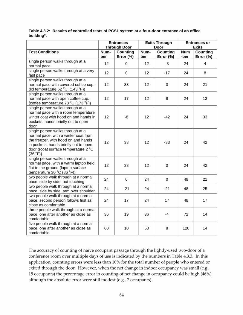
Table 4.3.2: Results of controlled tests of PCS1 system at a four-door entrance of an office building*.

Entrances Through Door

Exits Through Door

Entrances or Exits

Test Conditions

Num-ber

Counting Error (%)

Num-ber

Counting Error (%)

Num-ber

Counting Error (%)

single person walks through at a normal pace 12 0 12 -8 24 4

single person walks through at a very fast pace 12 0 12 -17 24 8

single person walks through at a normal pace with covered coffee cup. {lid temperature 62 oC (143 oF)}

12 33 12 0 24 21

single person walks through at a normal pace with open coffee cup. {coffee temperature 78 oC (173 oF)}

12 17 12 8 24 13

single person walks through at a normal pace with a room temperature winter coat with hood on and hands in pockets, hands briefly out to open door

12 -8 12 -42 24 33

single person walks through at a normal pace, with a winter coat from the freezer, with hood on and hands in pockets, hands briefly out to open door ({coat surface temperature 2 oC (36 oF)}

12 33 12 -33 24 42

single person walks through at a normal pace, with a warm laptop held flat to the ground {laptop surface temperature 30 oC (86 oF)}

12 33 12 0 24 42

two people walk through at a normal pace, side by side, not touching 24 0 24 0 48 21

two people walk through at a normal pace, side by side, arm over shoulder 24 -21 24 -21 48 25

two people walk through at a normal pace, second person follows first as close as comfortable

24 17 24 17 48 17

three people walk through at a normal pace, one after another as close as comfortable

36 19 36 -4 72 14

five people walk through at a normal pace, one after another as close as comfortable

60 10 60 8 120 14

The accuracy of counting of naïve occupant passage through the lightly-used two-door of a conference room over multiple days of use is indicated by the numbers in Table 4.3.3. In this application, counting errors were less than 10% for the total number of people who entered or exited through the door. However, when the net change in indoor occupancy was small (e.g., 15 occupants) the percentage error in counting of net change in occupancy could be high (46%) although the absolute error were still modest (e.g., 7 occupants).

64

Table 4.3.3: Counting accuracy of PCS1 system with naïve occupants passing through a two-door entrance to a conference room.

Entrance Through Door (s) Exit Through Door (s) Entrances Minus Exits

Actual Counted Error Actual Counted Error Actual Counted Error 53 57 7.5% 68 65 -4.4% -15 -8 7 (-46%)

The accuracy of counting of naive occupant passage through the four-door entrance of the office building is indicated by the numbers in Table 4.3.4. Because accuracy appeared to be reduced when the floor below the thermal sensors was illuminated and heated by sunlight, data were compiled for time periods with and without impingement of direct sunlight (determined visually) on the floor beneath the sensors. With no direct sunlight impinging on the floor, the errors in counting the number of people who entered or exited through the door were 13% or less. With direct sunlight on this section of floor, these errors were as high as -26%. As in the single door installation, when the net change in indoor occupancy was small the percentage error in counting of net change in occupancy was high (54%).

Table 4.3.4: Counting accuracy of PCS1 system with naïve occupants passing through a four-door door entrance to an office building.

Sunlight* Entrance Through Doors Exit Through Doors Entrances minus Exits

Actual Counted Error Actual Counted Error Actual Counted Error No 149 168 13% 180 194 8% -31 -26 5 (-16%) Yes 110 81 -26% 75 65 -13% 35 16 -19 (-54%)

* Direct sunlight impinging on floor beneath thermal sensors 4.3.2. People Counting System Number 2 Table 4.3.5 provides a compilation of results of counting accuracy of PCS2 with controlled challenges at the single-door entrance to Conference Room 1. There were no counting errors when single persons walked through the door at a normal pace, even when carrying cups of hot coffee or warm laptop computers. The counter failed to detect people wearing a room temperature winter coat with hood over their head and their hands in the pockets, but detected people without error when the winter coat had just been removed from a freezer. When a single person walked through the door at a very fast pace, the counter failed to register a count 25% of the time. When two people walked side-by-side through the door simultaneously, the counter normally registered only a one-person change in count. When three or five persons walked through the door following each other as closely as comfortable, the system under counted by 40% on average. The results of controlled challenges of PCS2 installed at the entrance door of Room 3 are provided in Table 4.3.6. The results are similar to those discussed above, but with better

65

counting accuracy when a single person walked very quickly through the door (no errors) and when three or five person walked through the door at a normal pace following each other as closely as comfortable.

Table 4.3.5: Results of controlled tests of PCS2 at a single interior door entrance to Conference Room 1, the numbers are averages of three repeated challenges.

Test Conditions

Room No.

Cor-rect

Count

Entrances Through Door

Exits Through Door

Entran-ces or Exits

Avg. Count

Count- ing Error (%)

Avg. Count

Count-ing

Error (%)

Count-ing

Error (%)

single person walks through at a normal pace 1 1 1 0% 1 0% 0%

single person walks through at a very fast pace 1 1 0.67 -33% 0.83 -17% -25%

single person walks through at a normal pace with covered coffee cup

1 1 1 0% 1 0% 0%

single person walks through at a normal pace with open coffee cup

1 1 1 0% 1 0% 0%

single person walks through at a normal pace with a room temperature winter coat with hood on and hands in pockets

1 1 0 -100% 0 -100% -100%

single person walks through at a normal pace, with a winter coat from the freezer, with hood on and hands in pockets

1 1 0.67 -33% 1 0% -17%

single person walks through at a normal pace, with a warm laptop computer held flat to the ground

1 1 1 0% 1 0% 0%

two people walk through at a normal pace, side by side, not touching

1 2 1 -50% 1 -50% -50%

two people walk through at a normal pace, side by side, arm over shoulder

1 2 1 -50% 1 -50% -50%

two people walk through at a normal pace, second person follows first as close as comfortable

1 2 0.67 -67% 1 -50% -58%

three people walk through at a normal pace, one after another as close as comfortable

1 3 1.33 -56% 2 -33% -44%

five people walk through at a normal pace, one after another as close as comfortable

1 5 2.83 -43% 3.5 -30% -37%

66

Table 4.3.6: Results of controlled tests of PCS2 at a single interior door entrance to room Room 3. The numbers are averages of three repeated challenges.

Test Conditions

Confer-ence Room No.*

Cor-rect

Count

Entrances Through Door

Exits Through Door

Entran-ces or Exits

Avg. Count

Count- ing Error (%)

Avg. Count

Count-ing

Error (%)

Count-ing

Error (%)

single person walks through at a normal pace 3 1 1 0% 1 0% 0%

single person walks through at a very fast pace 3 1 1 0% 1 0% 0%

single person walks through at a normal pace with covered coffee cup

3 1 1 0% 1 0% 0%

single person walks through at a normal pace with open coffee cup

3 1 1 0% 1 0% 0%

single person walks through at a normal pace with a room temperature winter coat with hood on and hands in pockets

3 1 0 -100% 0.67 -33% -67%

single person walks through at a normal pace, with a winter coat from the freezer, with hood on and hands in pockets

3 1 0.67 -33% 1 0% -16%

single person walks through at a normal pace, with a warm laptop computer held flat to the ground

3 1 1 0% 1 0% 0%

two people walk through at a normal pace, side by side, not touching

3 2 1 -50% 0.67 -67% -58%

two people walk through at a normal pace, side by side, arm over shoulder

3 2 0.83 -58% 0.83 -58% -58%

two people walk through at a normal pace, second person follows first as close as comfortable

3 2 1.83 -8% 2 0% 0%

three people walk through at a normal pace, one after another as close as comfortable

3 3 3 0% 3 0% 0%

five people walk through at a normal pace, one after another as close as comfortable

3 5 5 0% 4.67 -6% -3%

*Room was size of a small meeting room but used for offices

67

The accuracy of counting of naïve occupant passage through the single door of Conference Room 1 is indicated by the numbers in Table 4.3.7. Data are provided for 1.0 to 1.5 hour periods on four dates. Excluding data from a period when people were standing in the doorway, the errors in total counts of people entering or exiting the conference room ranged from 0% to -14% and averaged -5%. These errors in total counts reflect some over counting counteracted by some undercounting, thus, the percentage of counting events in which an error occurred was higher (0% to 20% with an average of 8%). On one date, there was a period in which people stood for an extended period in the doorway because the meeting room was full. Total count errors were +29% for people entering and -50% for people exiting during this period but the number of imperfect accounts was as high as 171% of the correct count.

Table 4.3.7: Counting accuracy of PCS2 with naïve occupants passing through single-door entrances to Conference Rooms 1 and 2.

Room 1 1 1 1 1 1 2

Time Period 9/9 9/11 10/6 10/7 (no

standing in door)

10/7 (with

standing in door)

9/9 – 10/7 All Periods

(no standing in

door)

12/18

Entrances Into Room Correct count 20 45 27 62 7 154 31 Counted 17.5 44.5 27 60 9 149 30 Error % -13% -1% 0% -3% 29% -3% -3% Missed full counts 1 1 0 2 2 4 0 False full counts 0 0 0 0 4 0 0 Undercounts by 0.5 3 0 0 0 3 3 2 Over counts by 0.5 0 1 0 0 3 1 0 Imperfect counts* % 20% 4% 0% 3% 171% 5% 6% Exits from Room Correct count 16 33 29 46 3 124 37 Counted 16 31.5 29 39.5 1.5 116 38 Error % 0% -5% 0% -14% -50% -6% 3% Missed full counts 0 2 0 6 1 8 0 False full counts 0 1 0 0 0 1 1 Undercounts by 0.5 1 1 0 1 1 3 2 Over counts by 0.5 1 0 0 0 0 1 1 Imperfect counts* % 12% 12% 0% 15% 67% 10% 14% Entrances or Exits Correct count 36 78 56 108 10 278 68 Counted 33.5 76 56 99.5 10.5 265 68 Error % -7% -3% 0% -8% 5% -5% 0% Imperfect counts* % 17% 8% 0% 4% 93% 15% 10% * Percentage of total events in which a counting error was noted. An event is the passage on one or more persons simultaneously or in close succession through the door, followed by a period with no persons passing through the door.

68

The accuracy of counting of naïve occupant passage through the single door of Conference Room 2 is indicated by the numbers in right most column of Table 4.3.7. On this date, no occupants stood in the door, counting errors were -3% and 3% for people entering and exiting the room, respectively, and imperfect counts were 10% of total counts.

4.4. Discussion

4.4.1. People Counting System Number 1 This pilot study of the PCS1 indicates that counting accuracy in some situations can be relatively high with errors on the order of 10%. However, relatively high counting errors occurred in the following demanding situations: 1) people carrying cups of hot coffee; 2) people following very closely behind each other when they pass through the door; 3) people in physical contact when passing through a doorway; 4) people wearing a room temperature winter coat with hood over their head, and 5) direct sunlight heating the floor located beneath the thermal sensors. The third and fourth of these situations are likely to occur infrequently, at least in most California climates. One could avoid using the PCS1 at locations where direct sun may heat the floor beneath the thermal sensors and the manufacturer indicated that changes in the type of floor matt or moving the detection lines further indoors from the door might have reduced these errors. In planning the testing of PCS1 for office building applications, the required minimum sensor height of 3.05 m made the system impractical for many building and conference room entrances. The manufacturer is developing a system that can be installed at a lower height, but this system was not evaluated.

4.4.2. People Counting System Number 2 In the controlled challenges of PCS2, counting accuracy was high when single individuals passed through the doorway at a normal pace. Carrying warm objects such as hot coffee or a warm laptop computer did not lead to counting errors. The counter often did not detect a person wearing a room temperature winter coat with hood over their head, but such events are likely very rare for interior doorways. In the first set of controlled tests, there was a substantial undercounting in some highly challenging events such as persons walking through the door at a very fast pace, two people passing through the door simultaneously, and people passing through a door sequentially as closely as comfortable. The accuracy in some of these situations was higher in the second set of controlled challenges. These controlled tests were performed with volunteers as subjects who differed between the two sets of controlled experiments. The results may have differed because the subjects in the first and second set of controlled tests walked at different speeds or with different distances from others. Additionally, as discussed previously, the start threshold was modified between the two sets of controlled tests. The accuracy of counting naïve occupants as they entered or exited Conference Room 1 and Room 2 was generally high, suggesting that the highly challenging events noted above are rare,

69

but more data are necessary before drawing this conclusion. However, the counter was found to be unsuitable for situations in which people stood in the doorway. In the present studies, this occurred when all seats of the conference room were utilized and a seminar presentation was underway. This situation was not encountered in tests of PCS1. PCS2 was easy to install and, based on the installation instructions, is usable in most interior doorways. The system does require that the building have a BACnet communication system, which limits its applicability in the current building stock. 4.4.3. General Observations This pilot testing of people counting systems has several limitations that prevent any firm conclusions about the suitability of these systems for providing a control signal for demand controlled ventilation. The tests involved only a few sensors, new sensors, a few installation sites, and limited periods of testing. Also, with additional experience the positions of the “lines” that subjects must cross to trigger a count might be adjusted to improve accuracy of PCS1 and the aforementioned settings might be changed to improve the accuracy of PCS2 for specific applications. Based on the pilot findings, it is clear that both counting system have limitations and would need to be used only at appropriate sites and where the demanding situations that led to counting errors were rare. In evaluation of the utility of these people counting systems for demand controlled ventilation one must keep in mind the advantages and disadvantages of people counting that were discussed in the introduction to this report and that that the widely used alternative sensors for demand controlled ventilation (low cost carbon dioxide sensors) often have large errors. No costs were available for the prototype PCS2. The cost of people-counting-based demand controlled ventilation with PCS1, relative to the cost of CO2-based demand controlled ventilation, will depend on the application. The price of the counting hardware for a single door entrance was $1450 while unit costs for single-point CO2 sensors are typically $300 to $500. The California Title 24 code requires a minimum of one sensor per 930 m2 of floor area where demand controlled ventilation is employed. Thus, CO2 sensor costs will be substantially lower for most small or moderate-size rooms if the minimum number of CO2 sensors are installed. However, for full building applications the costs of CO2 sensors at one or more sensor per 930 m2 of floor area could exceed the cost of people counting hardware. Installation costs per sensor should be similar for both types of sensors. People-counting-based demand controlled ventilation systems require a measurement system for the outdoor air intake rate which can be costly and inaccurate. CO2-based demand controlled ventilation is normally utilized without a system for measuring outdoor air intake flow rates, although, because such measurement systems are absent, minimum ventilation rates per unit floor area may often be poorly controlled. The relative costs will also depend on sensor lifetimes, which are currently unknown for both people counters and CO2 sensors. Finally, the effectiveness of the systems in controlling minimum ventilation rates will have a large impact on their cost effectiveness. Field studies have found that many of the CO2 sensors used for demand controlled ventilation have large errors (Fisk et al. 2009). Thus, CO2-based demand controlled ventilation is frequently not

70

providing the desired level of control of ventilation rates. This scale and scope of this pilot study was too small for firm conclusions about the energy savings potential of demand controlled ventilation based on people counting; however, the findings from this pilot study are sufficiently promising to indicate that further investigations of people counting are warranted.

4.5. Conclusions

The two people counting systems had high counting accuracies, with errors typically less than 10%, for typical counting events. However, counting errors were high in some highly challenging situations. Counting errors can be very high if people stand in the zone where the counters detect moving people. Both counting system have limitations and would need to be used only at appropriate sites and where the demanding situations that led to counting errors were rare.

The requirement for a high sensor height substantially limits the applicability of PCS1. The manufacturer reported that they were developing a system that can be installed at a lower height.

This scale and scope of this pilot study was too small for firm conclusions about the energy savings potential of demand controlled ventilation based on people counting; however, the findings from this pilot study are sufficiently promising to indicate that further investigations of people counting are warranted.

71

CHAPTER 5: Recommended Changes to Specifications for Demand Controlled Ventilation in California’s Title 24 Building Energy Efficiency Standards

5.1. Background

The research described in Chapters 2-4 has implications for the specifications pertaining to demand controlled ventilation in section 121 of the California Title 24 Standard (California Energy Commission 2008). Consequently, this document suggests possible changes in these specifications based on the research findings. The suggested changes in specifications were developed in consultation with staff from the Iowa Energy Center who evaluated the accuracy of new CO2 sensors in laboratory-based research (National Buildings Controls Information Program 2009). In addition, staff of the California Energy Commission, and their consultants in the area of demand controlled ventilation, provided input for the suggested changes in specifications.

5.2. Existing Specifications in Title 24 for Demand Controlled Ventilation

Appendix B reproduces verbatim the existing specifications for demand controlled ventilation in Title 24 and associated appendices. Key specifications relevant to this document are described in the following list:

1. Demand controlled ventilation is required for spaces that have an air economizer; a design occupant density, or a maximum occupant load factor for egress purposes greater than or equal to 25 people per 1000 ft2 (40 square foot per person); and that are either single zone systems with any controls; or multiple zone systems with direct digital controls to the zone level. There are exceptions to this requirement for certain types of spaces including as classrooms, call centers and medical facilities.

2. For each system with demand controlled ventilation, CO2 sensors must be installed in each room with no less than one sensor per 10,000 ft² of floor space. CO2 sensors must be located in the room between 3 ft and 6 ft above the floor or at the anticipated height of the occupants heads.

72

3. CO2 sensors shall be certified by the manufacturer to be accurate within plus or minus 75 ppm at a 600 and 1000 ppm concentration when measured at sea level and 25°C, factory calibrated or calibrated at start-up, and certified by the manufacturer to require calibration no more frequently than once every 5 years. Upon detection of sensor failure, the system shall provide a signal which resets to supply the minimum quantity of outside air to levels required by Section 121(b)2 to the zone serviced by the sensor at all times that the zone is occupied.

4. The CO2 sensor(s) reading for each zone shall be displayed continuously, and shall be recorded on systems with DDC to the zone level.

The acceptance requirement for demand controlled ventilation system include a functional test demonstrating that economizer system dampers open and close as intended to high and low CO2 concentrations

5.3. Key related research results

This section briefly describes the key results of the California Energy Commission and U.S. Department of Energy supported research that serve as the technical underpinning for the subsequent recommended changes in the specifications for demand controlled ventilation in Title 24. These research findings are described in much greater detail in the following references (Fisk et al. 2009; Fisk et al. 2010; Hong and Fisk 2009) and in Chapters 2-4 of this document. Some of the text below was drawn directly from the cited documents.

5.3.1. CO2 measurement accuracy Studies of the accuracy of deployed CO2 sensors used for demand controlled ventilation in California indicate that a substantial fraction of CO2 sensors had errors greater than specified in Title 24. Forty seven percent of sensors had errors greater than 75 ppm at a concentration of 760 ppm and 40% of sensors had errors greater than 75 ppm at a concentration of 1010 ppm. A significant fraction of sensors have much larger errors, e.g., larger than 300 ppm. These concentrations of 760 and 1010 ppm are typical of the setpoint concentrations at which demand controlled ventilation systems increase outdoor air ventilation rates. Thus, overall many CO2 sensors do not meet accuracy requirements.”

Sensors from some specific manufacturers and with particular design features had a better average accuracy than other sensors. However, use of sensors only in these categories, while helpful, would not result in widespread compliance with the Title 24 accuracy requirements.

73

A significant number of sensors in all age categories had large errors. Thus, replacing sensors every few years also would not solve the accuracy problem.

Because the results obtained from energy management systems generally agreed well with results obtained from sensor displays, the measurement errors appear to be primarily a consequence of sensor problems and not a consequence of errors in translating the sensor output signals to building energy management systems.

In analyses of a sample of nine faulty sensors, four of the sensors had an output signal that was essentially invariable with CO2 concentration, yet these sensors were still deployed, indicating that facility managers are not always aware of obviously faulty sensors.

In a laboratory-based study of the accuracy of 15 models of new single-location CO2 sensors performed by the Iowa Energy Center, many of the new CO2 sensors had errors greater than 75 ppm, and errors greater than 200 ppm were not unusual. Maximum errors of new sensors approached 500 ppm.

Pilot-scale studies of the accuracy of multi-location CO2 monitoring systems were too limited for firm conclusions about the accuracy of these systems; however, the limited results obtained were encouraging. The study results illustrate the advantage of incorporating a measurement of outdoor air CO2 concentration with each sensor – offset errors cancel out in the indoor-outdoor CO2 concentration difference. For widespread acceptance, it seems likely that the costs of these systems will need to be reduced.

Together, the findings from the laboratory studies of the Iowa Energy Center and the field studies supported by the California Energy Commission indicate that many CO2-based demand controlled ventilation systems will fail to meet the design goals of saving energy while assuring that ventilation rates meet code requirements.

5.3.2. Spatial variability of CO2 concentrations in occupied meeting rooms Multipoint measurements of CO2 concentrations in occupied meeting rooms were completed to provide information for locating the CO2 sensors in meeting rooms. The Title 24 standard requires that CO2 be measured between 0.9 and 1.8 m above the floor with no less than one sensor per 930 m2 of floor area. In some of the meeting rooms, concentrations at different wall-mounted sample points varied by more than 200 ppm and concentrations at these locations sometimes fluctuated rapidly. These concentration differences may be a consequence, in part, of the high concentrations of CO2 in the exhaled breath of nearby occupants. Because the results of the multipoint measurements varied among meeting rooms, this research does not result in definitive guidance for locating sensors in meeting rooms; however, the results suggest that measurements at return-air grilles may be preferred to measurements at wall-mounted locations. In four out of seven data sets, CO2 concentration at return-grille locations fell between the maximum and minimum of CO2 concentrations at wall-mounted locations and in five of seven data sets, the period average concentration at return grilles was within 10% of the period average concentration measured from sample points on walls.

74

5.3.3. Performance of optical people counters Pilot-scale studies evaluated the counting accuracy of two people counting systems that could be used in demand controlled ventilation systems, instead of CO2 sensors, to provide control signals for modulating outdoor air ventilation rates. The evaluations included controlled challenges of the people counting systems using pre-planned movements of occupants through doorways and evaluations of counting accuracies when naïve occupants (i.e., occupants unaware of the counting systems) passed through the entrance doors of the building or room. The two people counting systems had high counting accuracy accuracies, with errors typically less than 10%, for typical non-demanding counting events. However, counting errors were high in some highly challenging situations, such as multiple people passing simultaneously through a door. Counting errors, for at least one system, can be very high if people stand in the field of view of the sensor. Both counting system have limitations and would need to be used only at appropriate sites and where the demanding situations that led to counting errors were rare.

5.3.4. Energy savings potential from demand controlled ventilation in occupied meeting rooms National level data indicate that average minimum ventilation rates in offices are either 13 or 38 L/s-person. The different average minimum ventilation rates are the result of different measurement protocols but both values are well above the minimum ventilation requirement in California which is approximately 7 L/s-person. These numbers suggest potential energy savings from use of demand controlled ventilation in general offices to bring the average minimum ventilation rate into alignment with the Title 24 requirement. Modeling and cost analyses, performed to assess this potential, indicated that demand controlled ventilation would generally not be cost effective for general office spaces in California if existing office buildings have 13 L/s-person of ventilation but would often be cost effective if existing buildings have 38 L/s-person of ventilation.

5.4. Recommendations

Based on the research described above, many existing CO2-based demand controlled ventilation systems will fail to meet the design goals of saving energy while assuring that ventilation rates meet code requirements. However, the potential energy savings from properly operating demand controlled ventilation systems appear to be substantial in magnitude. Thus, it is appropriate to consider how the specifications for demand controlled ventilation in the Title 24 Standards could be changed in order to improve the performance of demand controlled ventilation systems. The following text describes recommended changes in specifications and a discussion of the recommendations. There is some overlap in the language within the various recommendations that should be removed if multiple overlapping recommendations are adopted.

75

5.4.1. Recommendation 1 5.4.1.1 Description of recommendation 1 CO2 sensors installed in new installations of demand controlled ventilation shall have inlet ports and written protocols that make it possible to calibrate the deployed sensors using CO2 calibration gas samples. The inlet ports must provide paths for introducing calibration gas samples into the sensors. The protocols must provide the guidance that a facility manager or building control system professional needs to check and, if necessary, adjust the sensors’ calibration’ using, at a minimum, two calibration gas samples. The calibration protocol shall specify that one calibration gas sample has a CO2 concentration between 950 and 1050 ppm, with the actual concentration of the calibration gas known within ± 2 percent. The protocol shall specify calibration with a second calibration gas concentration of either zero ppm CO2 or between 450 and 550 ppm CO2, with the actual concentration of the calibration gas known within ± 2 percent.

Exception: The inlet port and calibration protocol are not required if the sensor manufacturer or their agent maintains a sensor exchange program in which deployed sensors are replaced with new or used factory-calibrated sensors at least once per year.

5.4.1.2 Discussion of recommendation 1 The accuracy of CO2 sensors used for demand controlled ventilation must be improved if demand controlled ventilation systems are to provide the intended energy and indoor environmental quality benefits. Based on the previously-described research (Fisk et al. 2010), restricting the allowable sensor designs will not assure widespread compliance with the Title 24 accuracy requirements. CO2 measurement accuracy cannot be assured if sensors are not calibrated. Many sensors utilized today cannot practically be calibrated after deployment due to the absence of an inlet port and/or calibration protocol. This recommended change in Title 24 specifications would enable calibrations of all deployed sensors unless the manufacturer maintains a sensor exchange program in which deployed sensors are replaced with new or used factory-calibrated sensors at least once per year. The recommended changes in specifications would also provide incentives to manufacturers to offer sensor exchange programs.

Manufacturer’s of sensors that already meet these requirement are likely to be supportive of the change in specifications. Many of the existing CO2 sensors marketed for demand controlled ventilation do not meet the requirements in this recommendation, thus, substantial industry opposition to the changes should also be expected. Also, it is important to note that making it possible to calibrate deployed sensors does not assure that the calibrations will actually be performed. A significant fraction of CO2 sensors already meet these requirements; however, in the field studies by the authors no facility manager reported that they had calibrated their CO2 sensors subsequent to the initial sensor installation period. It is hoped that as the results of research demonstrating large CO2 measurement errors become known, calibrations will become more common.

No analyses have been performed to determine if sensors meeting the requirements of Recommendation 1 have a significantly higher cost; however, compliant sensors are commonly

76

used today suggesting that incremental costs, if any, are modest. The resulting energy savings will reduce energy costs by an amount that has not been determined.

An alternative or supplement to Recommendation 1 would be to establish an independent sensor validation program that periodically evaluates samples of sensors of various types. A one-time sensor evaluation after a new sensor is introduced into the market may not be adequate. Only sensors on a list of those that pass this program would be compliant with Title 24 requirements. It would be best if the program costs were not paid by sensor manufacturers so that the testing organization is not beholden to the sensor companies. Such a program would be expected to improve at least the initial accuracy of CO2 sensors used for demand controlled ventilation, it would not rely on facility managers to implement calibrations, and it would not restrict any sensor design features. A main drawback is the difficulty of establishing and financing of the independent sensor validation program. In addition, because sensor calibrations may change over the life of the sensor, such a sensor validation program would not assure that sensor accuracy is maintained.

5.4.2. Recommendation 2 5.4.2.1 Description of recommendation 2 Within 60 days after installation in a building, all CO2 sensors installed for demand controlled ventilation shall be calibrated, using the manufacturer’s recommended protocol, to assure CO2 measurements are accurate within ± 75 ppm. The protocol must check and, if necessary, adjust the sensor’s calibration using, at a minimum, two calibration gas samples, one with a CO2 concentration between 950 and 1050 ppm and the second with a CO2 concentration of either zero ppm or between 450 and 550 ppm. The concentration of the CO2 in the calibration gases shall be known within ± 2 percent.

Exception: This calibration is not required if the sensor is provided with documentation demonstrating that a comparable calibration was implemented for the specific sensor within the past 90 days and that the sensor is accurate within ± 75 ppm at 500 ± 50 and 1000 ± 50 ppm CO2 concentrations when measured at sea level and 77 oF (25°C).

5.4.2.2. Discussion of recommendation 2 The accuracy of CO2 sensors used for demand controlled ventilation must be improved if demand controlled ventilation systems are to provide the intended energy and indoor environmental quality benefits. Based on the previously-described research (Fisk et al. 2010), restricting the allowable sensor designs will not assure widespread compliance with the Title 24 accuracy requirements. The studies of the accuracy of new CO2 sensors by the Iowa Energy Center (National Buildings Controls Information Program 2009) demonstrated that existing Title 24 requirements do not assure that a large majority of new CO2 sensors meet the accuracy requirements of Title 24. This recommended specification, if enforced, would assure that new CO2 sensors receive a calibration and are accurate within ± 75 ppm when initially installed or

77

shortly thereafter. Because sensor calibrations may change over the life of the sensor, such a sensor validation program would not assure that sensor accuracy is maintained.

The automated background calibration features present in many of the existing CO2 sensor technologies will adjust sensor calibrations based on the lowest CO2 concentrations experienced. After initial sensor deployment, the accuracy of CO2 measurements may improve (or occasionally degrade) over a period of a few weeks. Thus, for sensors with an automated background calibration feature, it may be preferable to perform the on-site calibration after 30 days of deployment. Manufacturer’s protocols should specify when on-site calibrations should be performed after initial sensor deployment.

This requirement will increase the cost of installing demand controlled ventilation systems by an amount that has not been determined. The resulting energy savings will reduce energy costs by an amount that has not been determined.

5.4.3. Recommendation 3 5.4.3.1 Description of recommendation 3 All CO2 sensors shall have a continuously-readable visual display of the current CO2 concentration on the sensor. Manufacturer’s may provide a cover that makes the display accessible to facility managers but not to other building occupants.

5.4.3.2 Discussion of recommendation 3 Displays of the currently measured CO2 concentrations on the CO2 sensors may make facility managers more aware of faulty sensors that require calibration or replacement. The research described above has shown that sensors that do not respond to changes in CO2 concentrations and sensors with very large easily recognizable measurement errors are sometimes deployed in buildings (Fisk et al. 2010). Displays of CO2 concentration should also make it easier for controls contractors and facility managers to assure that CO2 concentration at the energy management and control system matches the concentration at the sensor, e.g. make it easier to detect and avoid signal processing errors. Finally, displays will facilitate the process of calibrating deployed CO2 sensors.

5.4.4. Recommendation 4 5.4.4.1. Description of recommendation 4 Change the existing specification in Title 24 that reads as follows “CO2 sensors shall be located in the room between 3 ft and 6 ft (0.9 and 1.8 m) above the floor or at the anticipated height of the occupants heads” to “CO2 sensors shall be located in the room between 3 ft and 6 ft (0.9 and 1.8 m) above the floor or at the anticipated height of the occupant’s heads or in the return air duct if the return air duct contains only air from the room for which demand controlled ventilation is implemented. Sensors shall not be installed in return air ducts if the room has a ventilation system designed to produce a displacement air flow pattern between the floor and

78

the ceiling or if the ceiling is more than 14 ft (4.3 m) above the floor. Sensors shall not be installed in return-air plenums or at the plane of the return-air grille.”

5.4.4.2. Discussion of recommendation 4 The research summarized above found that CO2 concentrations at different locations on walls of meeting rooms could differ by more than 200 ppm and fluctuate considerably with time (Fisk et al. 2010). The study was too small for definitive conclusions; however, relative to a CO2 measurement at a single location on a meeting room wall, a measurement in a return air duct appears to be as representative, and possibly more representative, of the average CO2 concentration in the room. CO2 sensors installed on walls may be exposed to air from within wall cavities if the room is slightly depressurized relative to the wall cavity because the electrical wiring for wall-mounted sensors normally extends through an unsealed hole in the wall behind the sensor. Also, wall- mounted sensors may occasionally be exposed to the jets of low-CO2 supply air as these jets can flow across ceilings and down walls. The existing prohibition against duct-mounted sensors was likely motivated by concerns that low-CO2 supply air exiting a ceiling mounted supply air diffuser may short circuit to a return grille, causing the return air CO2 concentration to be substantially lower than the average concentration in the room. While such short circuiting can occur, studies of indoor air flow made using tracer gases in rooms with traditional high velocity air supplies indicate that substantial short circuiting is not common (Fisk and Faulkner 1992). Measurable short circuiting is most likely when the supply air is used for heating (Fisk et al. 1997) and prolonged heating of meeting rooms with a high occupant density, where demand controlled ventilation is required, may be uncommon. Thus, while there is not enough evidence to justify requiring that CO2 sensors be installed in return ducts as opposed to on walls, there is also not sufficient justification to prohibit locating CO2 sensors in return ducts. The prohibition against duct-mounted sensors when the ceiling is more than 4.3 m above the floor is a judgment-based precaution as concentration differences between the occupied zone and the ceiling may be larger when the ceiling height is large. No data were identified confirming that duct-mounted sensors are inappropriate in rooms with high ceilings.

5.4.5. Recommendation 5 5.4.5.1. Description of recommendation 5 Change the existing specification in Title 24 that reads as follows “For each system with demand control ventilation, CO2 sensors shall be installed in each room that meets the criteria of Section 121(c)3B with no less than one sensor per 10,000 ft² of floor space.” to “For each system with demand control ventilation, CO2 sensors shall be installed in each room that meets the criteria of Section 121(c)3B with no less than one sensor per 10,000 ft² of floor space. In addition to stand- alone sensors that measure the CO2 concentration at a single location, measurements may be performed with measurement systems that use tubing, valves, and pumps to measure at multiple indoor locations with a single CO2 sensor if data are available from each location at least once every 10 minutes.”

79

5.4.5.2. Discussion of recommendation 5 The purpose of this proposed change in Title 24 language it to make prospective users more aware of multi-location CO2 measurement systems which tend to use higher quality CO2 sensors and incorporate an outdoor air CO2 measurement, both of which can improve accuracy of determining the indoor-to-outdoor CO2 concentration differences. Pilot scale studies of the multi-location CO2 measurement systems were too limited for firm conclusions about system accuracy but the findings were encouraging (Fisk et al. 2010).

5.4.6. Recommendation 6 5.4.6.1 Description of recommendation 6 The required types of building spaces for which demand controlled ventilation is required in Title 24 should not be expanded to include general office spaces, however, demand controlled ventilation should continue to be optional for general office spaces.

5.4.6.2. Discussion of recommendation 6 Model results, summarized above, evaluated the potential energy savings and cost effectiveness of implementing demand controlled ventilation in general office spaces. Given the model findings and the uncertainty about minimum ventilation rates in the existing office building stock, there is a large uncertainty about the cost effectiveness of demand controlled ventilation in general office spaces in California climates. Consequently, we do not recommend requiring demand controlled ventilation in general office spaces.

5.4.7. Recommendation 7 5.4.7.1 Description of recommendation 7 At this time, Title 24’s specifications pertaining to demand controlled ventilation should not be modified to allow use of optical people counting, in place of CO2 sensors, to provide the control signal for demand controlled ventilation.

5.4.7.2 Discussion of recommendation 7 Pilot scale studies were completed to evaluate the performance of two optical people counting systems potentially suitable for use in demand controlled ventilation systems (Fisk and Sullivan 2009). The counting errors were generally small, indicating the long-term potential of applying people counting for demand controlled ventilation. However, in some highly demanding situations counting errors were large. Further research is needed, and product improvements may be necessary, before one can be confident that optical people counting systems provide a sufficiently accurate count of people to serve as a control signal for demand controlled ventilation.

80

5.5. Discussion

Changes in demand controlled ventilation sensor technologies and practices are necessary if demand controlled ventilation is to consistently save energy and assure adequate ventilation. Based on the results of a multi-faceted research effort, this document describes five recommended changes to the specifications in Title 24 for demand controlled ventilation and makes two recommendations to not change aspects of Title 24. Enacting the suggested recommendations should help demand controlled ventilation to achieve its potential but they will definitely not eliminate all sensing problems in demand controlled ventilation systems. Further research to evaluate and develop alternatives to the widely used low-cost single location non-dispersive infrared CO2 sensor may be needed if demand controlled ventilation is to reach its full potential. Although the recommendations in this report were developed with input from the California Energy Commission and the Iowa Energy Center, a thorough evaluation all of the ramifications of implementing these recommendations was beyond the scope of the supporting research project. Consequently, the California Energy Commission will need to further evaluate these recommendations.

81

CHAPTER 6: Relationship of Classroom Ventilation Rates with Student Absence 6.1. Background

The supply of outdoor air ventilation into a building decreases the indoor air concentrations of pollutants generated indoors. Increased ventilation, however, also increases energy costs. Indoor-generated pollutants include chemical emissions from the building and its physical contents, with potential irritant, toxic, allergenic, or odorous properties, and also potentially infectious and odorous emissions from people. Historically, VR guidelines were set to control odors from occupants for the satisfaction of visitors, based on laboratory studies (Seppanen et al. 1999). Accumulating evidence, mostly from offices, now suggests that lower VRs in buildings are associated with increases in a variety of adverse health effects, such as infectious respiratory disease, acute symptoms, or impaired cognition or performance (Seppanen et al. 1999). Evidence also shows that a substantial proportion of classrooms do not provide the minimum rates of ventilation specified in standards (Daisey et al. 2003). However, the scientific evidence on the relationships between VRs and specific human health outcomes is still very limited, especially for schools. School-age children spend 15 to 25% of their time indoors at school, more than in any other indoor environment except the home (68%) (Klepeis et al. 1996). It is important to determine how VRs influence student health, in order to develop minimum ventilation standards for classrooms that strike a balance between health and the energy costs of providing ventilation

Available limited evidence suggests that lower ventilation rates (VRs) in offices, schools, and dormitory rooms are associated with increased illness absence (Seppanen et al. 1999; Sun et al. 2011). Only one available study, however, provides information on relationships between VRs in classrooms and the health of students, as indicated by total absence. Shendell et al. (2004) reported that higher classroom ventilation rates were associated with a substantial reduction in student absence. This study, however, used rough measurements for analyses – short, one-time measurements of CO2 in each classroom as proxies for VRs throughout the school year, and an outcome of total absence, which includes illness absence but also other types of absence unlikely to be influenced by VR. This paper reports findings of a study, conducted in California elementary schools, on the associations between ventilation rates (VRs) in classrooms and illness-related school absences, using illness absence as an indicator of health effects sufficiently severe to require staying home from school. Illness absence can be related to respiratory infections, asthma, allergies, gastrointestinal infections, or other disease. The primary hypothesis was that decreased VRs in

82

classrooms would be associated with increased illness absences resulting from increased indoor airborne concentrations of respiratory virus and consequent increased exposure and infection. Such absences might also result to a lesser extent from other airborne agents related to asthma, allergies, or infectious gastrointestinal illness.

6.2. Methods

To provide improved estimates of relationships between classroom VRs and illness absence, information was collected from a large number of schools in three climate zones within California, over two school years, with sufficiently detailed data to estimate daily ventilation rates and daily illness-related absence by classroom. Web-connected CO2 sensors were installed in classrooms, allowing remote collection of real-time data for estimating daily ventilation rates. Data on student absence and demographic were obtained from the participating school districts. The associations of VRs with absence were quantified using statistical models that controlled for several potential confounding factors including socio-economic status, grade level, gender mix, and class size. (The energy costs of classroom ventilation and some financial implications to school districts and families from changes in absence rates were also estimated. These will be reported in Chapter 7.) 6.2.1. Sample design and selection for epidemiologic analysis The sample design started with aggregation of the 16 Building Climate Zones of the California Energy Commission (http://www.energy.ca.gov/maps/renewable/building_climate_zones.html) into a smaller number of climate regions with relatively homogeneous levels of heating and cooling degree-days (see Figure 6.3.1 for boundaries). Included in the study were three climate regions with large populations: South Coast (SC), with mild winters and warm summers; Bay Area (BA), with mild summers and winters; and Central Valley (CV), with cold winters and hot summers.

Within each selected climate region, the largest school district (by student enrollment) was identified and invited to participate in our study. If they were unable, or declined, to participate, the next largest school district was contacted, and this process continued until participation by an eligible district was arranged. An eligible school district needed to be willing and able to provide us with the following data:

• classroom-level daily illness-related absence data • non-identifiable annual student STAR Math and English scores for the students in the

monitored classrooms (for the current and prior years)

Within each participating school district, up to 10 elementary schools were selected. To include schools across a range of socioeconomic levels, schools in each district were first ranked by the percent of students who participated in the free or reduced price meals program, used as a surrogate for socioeconomic status ((http://www.cde.ca.gov/ds/sh/cw/filesafdc.asp, Categorical

83

Allocations & Audit Resolution, School Fiscal Services Division of the California Department of Education, accessed on date Sept 12, 2008). The distribution was divided into five quintiles, and the two largest schools per quintile selected for potential participation.

Eligible schools needed to meet the following criteria: • approval by their Principal to participate; • approximately six available 3rd, 4th, or 5th grade classrooms, in either permanent or

portable buildings, with wired Internet (Ethernet) connections; • school permission to allow mounting and connection to the Internet of one

environmental sensor in each study classroom and one sensor outside at the school, for the duration of the study (two school years);

• agreement by the school or school district to provide student data for study classrooms on both daily classroom-level illness-related absence, and annual individual-level but unidentifiable test scores including linked scores for the current and prior school years.

Within each participating school, approximately six classrooms, two each in 3rd, 4th, and 5th grade, were selected. Eligible classrooms needed to meet the following criteria:

• students spending most of the day in the same 3rd, 4th, or 5th grade classroom (rather than moving between multiple classrooms);

• single, not combination, grade classroom; • providing a general education curriculum, not a dedicated special education classroom.

Some participating classrooms, upon becoming ineligible during the study due to change in use, were replaced by alternate eligible classrooms when feasible; others were simply excluded going forward. Only data from eligible periods in each classroom were included in analyses. 6.2.2. Data variables for epidemiologic analysis 6.2.2.1. Student data The primary dependent variable was daily illness absence per classroom, included in analyses as a daily count. Total classroom enrollment data was available from all districts (approximated as the sum of all demographic counts per classroom), on a daily or less frequent basis; if available less than daily, data were backfilled to prior days using available enrollment counts untill a prior available periodic count. Other demographic data for students, as classroom-level proportions, were collected as potential covariates: participation in free or reduced price meal program, English-learner status, gifted status, special education status, gender, and race/ethnicity. Participation in free or reduced price meal program was included as an indicator of socioeconomic status, known to be associated with susceptibility to acute lower respiratory tract infections (Graham 1990).

84

6.2.2.2. Environmental data Installed in each participating classroom, and at one outdoor location at each school, were small (2 in x 4 in x 8 in) web/Ethernet-connected sensors (the “Nose” ™ by PureChoice) that measured carbon dioxide, temperature, and relative humidity in real time. The sensors transmitted the data to the manufacturer, as 5-minute averaged values of CO2 concentration (in parts per million, ppm), temperature (in degrees Fahrenheit, ºF), and relative humidity (in %). The nondispersive infrared CO2 sensors had a resolution of 10 ppm, a rated accuracy of the larger of 5% or 100 ppm, and a range of 0-2000 ppm. A computer server at Lawrence Berkeley National Laboratory downloaded these data directly from the PureChoice server daily and incorporated them into our database. Some sensors became inoperable for various periods or permanently during the study. When feasible, they were restarted or replaced, but this was not always possible. Missing sensor data were not estimated, so days in a classroom with missing sensor data contributed “missing values” for ventilation rate averages. Ventilation rate per person in each classroom each school day (Vo) in L/s per person was estimated in a mass balance model that used the indoor equilibrium concentration minus the corresponding outdoor CO2 (Equation {6.1}). The daily indoor equilibrium CO2 concentration for each classroom was calculated as the peak value of a 15-minute moving average of indoor CO2 values between 7 AM – 3 PM each day. The corresponding outside CO2 concentration, originally planned as the 60-minute outdoor averaged CO2 for the period ending at the midpoint of the selected 15-minute indoor period, was instead, due to errors in outdoor sensor readings, estimated in analyses as 400 ppm across all schools.

Vo = N/(Cmax15 − CO) 6.1

where

Vo = outdoor air flow rate per person (L/s person)

N = CO2 generation rate per person (see Note below)

Cmax15 = maximum 15-minute moving average classroom CO2 concentration

CO = outside CO2 concentration at time of Cmax30 (estimated as 400 ppm)

Note: The occupant CO2 generation rate (N) is based on a value of 0.0043 L/s for children (Haverinen-Shaughnessy et al. 2011).

Th eresearchers wished to define a lag period for constructing summary VR “exposure” metrics that would be likely to include relevant periods for the predominant diseases causing illness absence in schools. Available information on time lag after exposure to infectious respiratory disease until disease development, reviewed in determining metrics and models to use in analyses, showed a broad range of lag periods for different infectious agents (one day to three

85

weeks or more), (e.g., (Lessler et al. 2009). Little information was available about the relative contribution of specific disease agents in explaining school illness absence. Therefore, analyses were performed including different averaged periods of VR, all ending on the day before which illness absence was assessed. Based on the daily VR estimates, multiple aggregate VR metrics were constructed to use in analyses: average daily VRs over the 3-, 7-, 14-, and 21-day periods immediately prior to each day of modeled illness absence. Based on available knowledge, the 7-day period was chosen as the primary metric, including the estimated 95% upper confidence limit of the incubation period for multiple respiratory agents (rhinovirus, adenovirus, respiratory syncytial virus, influenza, parainfluenza, and coronavirus) (Lessler et al. 2009). The other metrics were considered exploratory. The 3-day metric included upper 95% confidence limits for only rhinovirus, influenza, and parainfluenza (Lessler et al. 2009).

6.2.2.3. Other covariates Other data variables available for analyses included the school district (SC, CV, BA); the school, grade level (3, 4, or 5); total classroom enrollment; building type (permanent or portable); type of ventilation (natural, mechanically ventilated without AC, or AC); day of week; and winter season (December through February).

6.2.3. Data management and epidemiologic analysis methods A database was created to combine data collected from the environmental sensors and school districts. Extensive data checking and cleaning were performed to insure that: data analyzed was only from eligible periods in each classroom (e.g., re eligible grade level and special education status); that measured CO2 levels were credible; and that reported illness absence data were plausible. Data from any classroom during ineligible periods were excluded. Only full school days were included in VR estimates; the periodically scheduled short (“minimum”) days at each school, on which peak CO2 was less likely to estimate a true equilibrium level and thus VR, were excluded, although illness absence on these days was included. Peak indoor CO2 levels considered implausible for equilibrium levels in occupied classrooms during a school day (below 600 ppm and above 7,000 ppm) were excluded. Because CO2 sensors outdoors turned out not to be stable with outdoor temperatures, all outdoor measurement data for CO2 were excluded. Descriptive data analyses were performed on the distribution of VRs and illness absence rates for all classrooms and selected subgroups. In analytical models at the classroom-day level, the relative change in absence per each change of 1 L/s per person of VR was estimated. A zero-inflated negative binomial (ZINB) models was used, due to extremely skewed data, with many values of 0 for daily illness absence in classrooms. Illness absence count on each classroom day was the outcome, with averaged VR periods as the primary exposure (3-, 7-, 14-, and 21- day exposure periods in separate models). Including illness absence counts per classroom as the outcome with a covariate of total enrollment per classroom was equivalent to analyzing for

86

proportion of illness absence. ZINB models contain two components: a zero inflation (ZI) model to estimate whether each observation could ever be non-zero, and a negative binomial (NB) model to estimate the values of the observations with a non-zero probability of being positive. Other covariates in the NB model included day of the week, grade level, class enrollment, proportion in school lunch program, and proportion male, and in the ZI model, day of the week, winter season, and class enrollment. Ventilation type was too closely confounded with school district for inclusion in models. Sixteen models were constructed: each of the four VR metrics used separately for each of three school districts and for all districts combined. Inference for the above models was performed using a bootstrap, by re-sampling the schools within districts. Based on the fitted ZINB models, illness absence was predicted at specific VR levels, in each school district and all districts combined. Such predictions are made for specific selected values of each independent variable included in the model. Where possible we chose values representing the mean of a variable in the entire dataset. The models predicted the illness absence at specific VR levels by district, for a 5th grade classroom with 26 children enrolled, of whom 52% were male, and 63% participated in the free or reduced price meals program, on a Monday in the non-winter season.

6.2.4. Estimating potential benefits of increased ventilation rates

Ttwo kinds of potential benefits associated with reduced illness absence were estimated for specific changes in VRs. It is difficult to estimate from available data all the benefits of reduced illness absences on decreased health care costs. First, financial benefits to school districts of decreased student illness absence were estimated. The State of California funds school districts based not on enrollment but on student attendance, also known as Actual Daily Attendance (ADA), which excludes any absences. Students generate revenue by contributing to the total ADA for a school year, by equation 6.2:

ΣRi = Σ (ADAi * RL) 6.2

where Ri = revenue generated for district by student (i) during a school year i ranges from 1 to the total number of students attending school in a district ADAi = actual daily attendance for student (i) = total days attended by student (i) in the

school year divided by the 180 days of school taught RL = revenue limit per ADA ($5,300 per pupil for unified school districts in 2009-10

(although varies by grade level and learning track) Also estimated were benefits to families resulting from decreased illness absence due to decreased costs from time taken off work or other tasks to care for their children. These

87

estimates used a previously reported approach based on employment and earnings data in the National Health Interview Survey (NHIS), an annual, nationally representative survey of U.S. households. Levy et al. (2011), using established cost-of-illness methods and NHIS data on children 6-11 years old attending school, estimated the value of a day for caregiver’s time for each child missing school. For employed caregivers, Levy et al. used self-reported daily earnings, or if unemployed, used the value of time for lost household production, according to the cost of hiring someone else to complete the household tasks. Estimates involved a number of conservative assumptions (Levy et al. 2011). The present analysis follows Levy in estimating that 69% of the caregivers were employed, with mean annual and daily earnings of $20,087 and $80; value of household production among unemployed caregivers was estimated at $51 daily. The overall averaged value of household production among families with employed or unemployed caregivers was 55.2+15.8 = $71 per day of child illness absence.

6.3. Results

Three school districts in California participated: one each in the SC, BA, and CV regions (see Figure 6.3.1). The researchers selected a subsample of 10 schools in the SC district and nine in the BA, but included all nine available elementary schools in the CV district. Within each school, the goal was to include 2 classrooms at each of the 3rd, 4th, and 5th grade levels, but the available classroom mix varied slightly from this in some schools. By the end of the study, valid data were collected in 28 schools, from 166 classrooms. Table 6.3.1 shows the types of buildings and types of ventilation in the studied classrooms for each school district. The classrooms included 107 in permanent buildings and 55 in portables; and 61 with natural ventilation only, 30 with mechanical ventilation without air conditioning (AC), and 30 with AC. While the BA district classrooms included a mixture of naturally ventilated, mechanically ventilated without AC, and AC, the SC classrooms included no AC, and the CV schools all had AC. Table 6.3.2 provides data on the distributions of estimated equilibrium indoor CO2 concentrations and estimated VRs in the study classrooms. Ventilation rates differed substantially across districts, with median VRs in the SC, BA, and CV districts of 7.0, 5.1, and 2.6 L/s per person, respectively. VRs varied most in the SC district, less in the BA, and relatively little in the CV, with ranges between the 5th and 95th percentiles for VR of 18.0, 12.2, and 5.1 L/s per person respectively. VRs also varied by building type, with medians in permanent and portable classrooms of 6.8 and 5.0 L/s per person respectively, and by ventilation type, with medians for natural, mechanical/no AC, and AC of 6.0, 7.6, and 2.8 L/s per person respectively. Table 6.3.3 provides descriptive data on the classrooms with valid data available for analyses. All enrolled schools were included except for four in Oakland. Average total enrollment across all studied classroom during the study was 2,358. Average student enrollment in each studied classroom was slightly lower in the BA district (25.9) than in the SC (27.3) or CV (26.3), with third grade enrollment, per classroom and overall in the study, smaller than the higher grades in all three districts. Slightly more males were included in each district. Almost three quarters

88

of the students participated in the National School Lunch Program (official name of the federal Free or Reduced Price Meal Program) in BA and CV, compared to about half in SC. Proportions of racial/ethnic categories varied across the districts: Asian/Pacific Islander, 7-33%; White, 14-38%; Black, 3-29%, and Latino, 20-51%. Analyses potentially included almost 35,000 classroom days (Table 6.3.3). Mean daily classroom proportions of illness absence ranged across districts from 2.11-2.53%, and across grades 3 to 5, were 2.54, 2.25, and 2.30%, respectively. Mean proportion of illness absence was higher in the winter months (December-February) within each district and overall. Median proportion of daily classroom illness absence in all categories (not shown) was 0.

Figure 6.3.1: Climate regions included.

89

Table 6.3.1: Descriptive information on selected study variables

District SC BA CV All Summer temperature warm mild hot --- Winter temperature mild mild cold --- Number of schools 10 9 9 28 Number of classrooms 59 52 51 162 Building type for classrooms

Proportion (number) in permanent buildings 59% (35) 81% (42) 59% (30) 66% (107) Proportion (number) in portable buildings 41% (24) 19% (10) 41% (21) 34% (55)

Ventilation type for classrooms Proportion (number) with natural ventilation 76 % (45) 31% (16) 0% (0) 37% (61) Proportion (number) with mechanical ventilation, no AC 24% (14) 31% (16) 0% (0) 19% (30) Proportion (number) with AC 0% (0) 38% (20) 100% (51) 44% (71)

Number of classroom days with ventilation rate data** 11,069 9,615 8,135 28,819 Approximate total enrollment in all 3rd, 4th, and 5th grade classrooms in studied school districts***

Third grade 10,000 4,000 1,000 15, 000 Fourth grade 10,000 4,000 1,000 15, 000 Fifth grade 10,000 4,000 1,000 15, 000

Abbreviations: AC, air-conditioning; BA, Bay Area; CV, Central Valley; SC, South Coast; VR, ventilation rate

** includes all those with valid VR data, although may not all be included in models; i.e., it includes all 28 schools and classrooms, even though some entire schools in BA were excluded from analyses.

*** i.e., whether studied or not; numbers rounded to nearest 1,000 to maintain anonymity of participating school districts; data source = http://www.ed-data.k12.ca.us/App_Resx/EdDataClassic/fsTwoPanel.aspx?#!bottom=/_layouts/EdDataClassic/profile.asp?Tab=0&level=06&reportnumber=16&county=50&district=75739 , accessed Apr 3, 2012

90

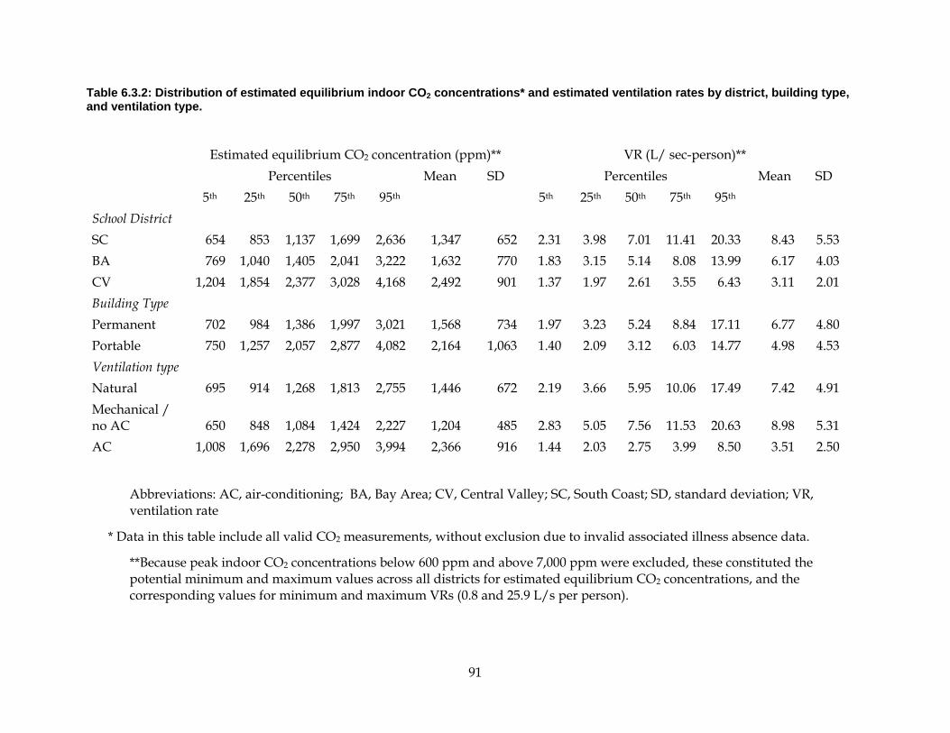
Table 6.3.2: Distribution of estimated equilibrium indoor CO2 concentrations* and estimated ventilation rates by district, building type, and ventilation type.

Estimated equilibrium CO2 concentration (ppm)** VR (L/ sec-person)** Percentiles Mean SD Percentiles Mean SD 5th 25th 50th 75th 95th 5th 25th 50th 75th 95th School District SC 654 853 1,137 1,699 2,636 1,347 652 2.31 3.98 7.01 11.41 20.33 8.43 5.53 BA 769 1,040 1,405 2,041 3,222 1,632 770 1.83 3.15 5.14 8.08 13.99 6.17 4.03 CV 1,204 1,854 2,377 3,028 4,168 2,492 901 1.37 1.97 2.61 3.55 6.43 3.11 2.01 Building Type Permanent 702 984 1,386 1,997 3,021 1,568 734 1.97 3.23 5.24 8.84 17.11 6.77 4.80 Portable 750 1,257 2,057 2,877 4,082 2,164 1,063 1.40 2.09 3.12 6.03 14.77 4.98 4.53 Ventilation type Natural 695 914 1,268 1,813 2,755 1,446 672 2.19 3.66 5.95 10.06 17.49 7.42 4.91 Mechanical / no AC 650 848 1,084 1,424 2,227 1,204 485 2.83 5.05 7.56 11.53 20.63 8.98 5.31 AC 1,008 1,696 2,278 2,950 3,994 2,366 916 1.44 2.03 2.75 3.99 8.50 3.51 2.50

Abbreviations: AC, air-conditioning; BA, Bay Area; CV, Central Valley; SC, South Coast; SD, standard deviation; VR, ventilation rate

* Data in this table include all valid CO2 measurements, without exclusion due to invalid associated illness absence data.

**Because peak indoor CO2 concentrations below 600 ppm and above 7,000 ppm were excluded, these constituted the potential minimum and maximum values across all districts for estimated equilibrium CO2 concentrations, and the corresponding values for minimum and maximum VRs (0.8 and 25.9 L/s per person).

91

Table 6.3.3: Demographic and illness absence data.

District All SC BA CV Number of Schools 10 5 9 24 Number of Classrooms 59 26 51 136 Building type for classrooms Proportion (number) in permanent buildings 0.59 (35) 0.88 (23) 0.59 (30) 0.65 (88) Proportion (number) in portable buildings 0.41 (24) 0.12 (3) 0.41 (21) 0.35 (48) Ventilation type for classrooms Proportion (number) with natural ventilation 0.76 (45) 0.12 (3) 0 0.35 (48) Proportion (number) with mechanical ventilation, no AC

0.24 (14) 0.38 (10) 0 0.18 (24)

Proportion (number) with AC 0 0.50 (13) 1.0 (51) 0.47 (64) Average enrollment per classroom (SD) 27.3 (5.6) 25.9 (5.0) 26.3 (4.8) 26.7 (5.3) Third grade 23 21 21 22 Fourth grade 29 28 29 29 Fifth grade 29 28 30 29 Average combined enrollment of included classrooms 1,401 561 1,089 2,358 Third grade 345 133 301 598 Fourth grade 541 216 393 892 Fifth grade 515 211 394 867 Average proportion male 0.52 0.52 0.52 0.52 Average proportion National School Lunch Program** 0.49 0.76 0.71 0.62 Average proportion Asian or Pacific Islander 0.28 0.33 0.07 0.22 Average proportion White 0.17 0.14 0.38 0.23

92

Average proportion Black 0.18 0.29 0.03 0.16 Average proportion Latino 0.38 0.20 0.51 0.38 Number of classroom days with illness absence data* 16,807 7,338 10,562 34,707 Mean daily classroom proportion (%) of illness absence (SD) 2.36 (3.2) 2.11 (3.4) 2.53 (3.3) 2.36 (3.3)

3rd grade 2.42 2.48 2.74 2.54 4th grade 2.38 1.61 2.53 2.25 5th grade 2.29 2.32 2.32 2.30 Winter season*** 2.84 2.32 2.95 2.75 Non-winter season 2.19 2.02 2.40 2.22

Abbreviations: SD, standard deviation

* based on all valid IA data eligible for inclusion in models; however, some classroom-days included in these data were not included in models if lacking necessary VR data

** official name of the national Free or Reduced Price Lunch Program

*** Winter is defined as the months of December, January, and February.

93

Table 6.3.4: Unadjusted IRR estimates* and 95% confidence intervals (CI)** from zero inflated negative binomial models for association between classroom ventilation rate (VR) metrics and daily classroom proportion of illness absence, per increase of 1 L/s per person VR in observed range of 1-20 L/s per person.

School District All

South Coast Bay Area Central Valley

VR averaging

period n IRR

(95% CI**)

p-value n IRR

(95% CI**)

p-value n IRR

(95% CI**)

p-value n IRR

(95% CI**)

p-value

3 days**

13,363 0.988 (0.980-0.997)

p=0.009

5,252 0.979 0.907-1.06

p=0.59

9,781 0.998 (0.979-1.02)

p=0.81

28,396 0.988 (0.978-0.997)

p=0.011

7 days** 14,318 0.986 (0.975-0.996)

p=0.008

5,742 0.974 0.889-1.07

p=0.58

10,120 0.987 (0.965-1.01)

p=0.26

30,180 0.985 (0.974-0.996)

p=0.007

14 days** 14,559 0.984 (0.973-0.996)

p=.008

5,955 0.978 0.876-1.09

p=0.70

10,378 0.989 (0.962-1.02)

p=0.43

30,892 0.985 (0.973-0.996) p=0.009

21 days** 14,664 0.984 (0.973-0.996)

p=0.008

6,106 0.978 0.866-1.10

p=0.72

10,438 0.980 (0.954-1.01)

p=0.14

31,208 0.984 (0.972-0.996)

p=0.008

Abbreviations: IRR, incidence rate ratio; L, liter; s, second, VR, ventilation rate;

* estimates are the relative (multiplicative) change in the outcome for each increase of one L/s per person

** bootstrapped

** ending on day prior to day on which illness absence assessed

94

6.3.1. Modeling results Table 6.3.4 provides unadjusted estimates (with no covariates in the ZI or NB components of models) and 95% CIs from the ZINB models, for the association between classroom VR metrics and daily classroom proportion of illness absence, from the specific district models and the combined district models. Table 6.3.5 provides the adjusted estimates, which were very similar to the unadjusted estimates. The model assumes a non-linear relationship in which the relative change per VR unit stays constant, but the absolute change decreases as VR increases. The interpretation of the adjusted estimates for VR in the ZINB model (estimates are of incident rate ratios is: if a classroom were to increase its VR by 1 L/s per person while holding all other variables in the model constant, the expected proportion of illness absence (equivalent to the count, when holding class size constant) would be multiplied by a factor equal to the coefficient. Estimates less than 1.0 indicate decreased illness absence. Changes in illness absence corresponding to multiple unit increases of VR are estimated by exponentiating the estimates accordingly. For each additional 1 L/s per person of VR, illness absence is estimated to be lower (Figure 6.3.2): for the SC, BA, and CV districts, by 1.0–1.3%, 1.2–1.5%, and 0.0–2.0%, respectively, and in the model for all districts combined, by 1.4-1.8%. Only estimates in the SC and combined district models had 95% CIs excluding the null. Numbers (n) of eligible classroom-day observations in models were approximately 56% and 37% lower, for BA and CV respectively, than for SC. Comparing estimates for the 7-day averaged VR metrics across the separate district models: for each additional 1L/ sec-person of VR, illness absence was estimated to decrease, for the 3-, 7-, 14-, and 21-day periods, by 0.0–1.2%, 1.0–1.5%, 0.9–1.3%, and 1.3–2.0%, respectively. There is a general tendency for these estimates to increase as the averaging period for VR increases, rather than peaking for the 7-day metric as hypothesized. Note that the three districts included were not selected to be representative of California districts, and results from the combined districts model may not be applicable to California school districts generally. There also may be unrecognized confounding in the combined models. For another set of covariates in the model – days of the week – the most illness absences in each district were reported on Mondays, followed by Fridays or Tuesdays, with the least on Thursdays or Wednesdays. Illness absences by grade varied across districts: in BA, they were highest in third grade, substantially lower in fifth grade, and lowest in fourth grade, but in SC and CV, they were slightly higher in 4th and 5th grades. Male gender was associated consistently with increased illness absence. Proportion of free or reduced price meals was not associated consistently across districts with illness absence, but in the combined model was associated with decreased illness absence. Figure 6.3.3 plots predicted counts of illness absence in the three districts and in the combined data, over the observed range of VRs, based on adjusted models using 7-day averaged ventilation rates and the baseline values of covariates specified in the footnote. The vertical bars

95

at the base of each plot show the VR values of data points on which that the plot was based. Table 6.3.6 provides example predicted data points for VR levels in L/s per person of 1, 5, 10, 15, and 20, and also 4.0 (the estimated mean VR for California K-12 classrooms – see Chapter 7), 7.1 (the minimum VR for classrooms specified in California Title 24), 6.7 and 7.4 (the minimum VRs for classrooms of grade 4-5 and 3, respectively, specified by the current ASHRAE standards (ASHRAE 2010)), and 9.4 (the minimum VR specified for offices in ASHRAE Standard 62-89 in 1989). Increasing VRs from the current mean level of 4 L/s per person to the current minimum required in California of 7.1 L/s per person would result in predicted absolute reductions in IA of 0.1-0.2% and predicted relative reductions of 3.4-4.8% (based on estimates from the 3 school districts studied). Further increasing VRs to 9.4 L/s per person would predict further absolute reductions of 0.1-0.2% and relative reductions ranging from 3.6-5.0%. Increasing VRs from current average levels to 9.4 L/s per person would lead to an approximate 7-10% predicted reduction in illness absences. Increasing average VRs from 4 to 20 L/s per person would reduce illness absence by an estimated 20.7 %.

96

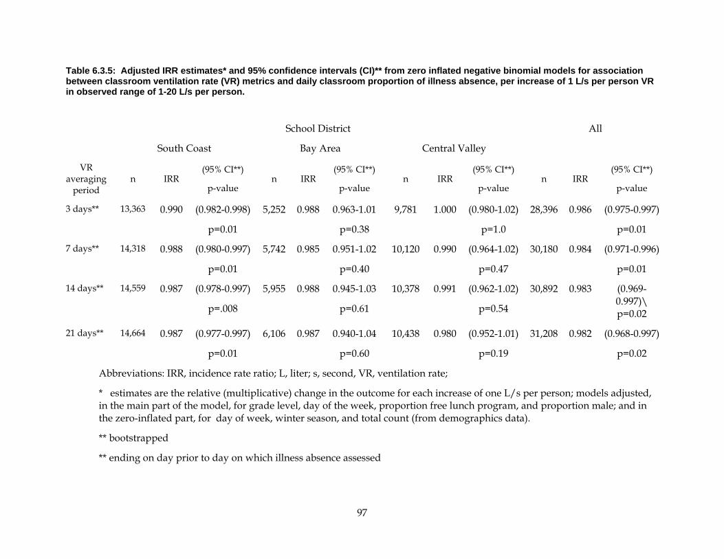
Table 6.3.5: Adjusted IRR estimates* and 95% confidence intervals (CI)** from zero inflated negative binomial models for association between classroom ventilation rate (VR) metrics and daily classroom proportion of illness absence, per increase of 1 L/s per person VR in observed range of 1-20 L/s per person.

School District All

South Coast Bay Area Central Valley

VR averaging

period n IRR

(95% CI**)

p-value n IRR

(95% CI**)

p-value n IRR

(95% CI**)

p-value n IRR

(95% CI**)

p-value

3 days**

13,363 0.990 (0.982-0.998)

p=0.01

5,252 0.988 0.963-1.01

p=0.38

9,781 1.000 (0.980-1.02)

p=1.0

28,396 0.986 (0.975-0.997)

p=0.01

7 days** 14,318 0.988 (0.980-0.997)

p=0.01

5,742 0.985 0.951-1.02

p=0.40

10,120 0.990 (0.964-1.02)

p=0.47

30,180 0.984 (0.971-0.996)

p=0.01

14 days** 14,559 0.987 (0.978-0.997)

p=.008

5,955 0.988 0.945-1.03

p=0.61

10,378 0.991 (0.962-1.02)

p=0.54

30,892 0.983 (0.969-0.997)\ p=0.02

21 days** 14,664 0.987 (0.977-0.997)

p=0.01

6,106 0.987 0.940-1.04

p=0.60

10,438 0.980 (0.952-1.01)

p=0.19

31,208 0.982 (0.968-0.997)

p=0.02

Abbreviations: IRR, incidence rate ratio; L, liter; s, second, VR, ventilation rate;

* estimates are the relative (multiplicative) change in the outcome for each increase of one L/s per person; models adjusted, in the main part of the model, for grade level, day of the week, proportion free lunch program, and proportion male; and in the zero-inflated part, for day of week, winter season, and total count (from demographics data).

** bootstrapped

** ending on day prior to day on which illness absence assessed

97

Figure 6.3.2: Estimated proportional change in illness absence with increase of 1 L/s per person of VR within the observed range of 1-20 L/s per person, using four ventilation metrics with different averaging periods*.

* ventilation averaging metrics end on day prior to day on which illness absence assessed

SC BA CV All

98

Figure 6.3.3: Predicted relationship between ventilation rate and proportion illness absence in three California school districts.

99

Table 6.3.6: Predicted proportion of illness absence at specified outdoor air ventilation rates, based on adjusted models* using 7-day averaged ventilation rates, in 3 California climate zones.

Predicted proportion of illness

absence

VR

(L/s per person)

VR

(cfm per person) District All

SC BA CV

1.0 2.1 0.029 0.043 0.029 0.031

4.0** 8.5 0.028 0.042 0.028 0.029

5.0 10.6 0.028 0.041 0.027 0.029

6.71 14.2 (132) 0.027 0.040 0.027 0.028

7.1*** 15 0.027 0.040 0.027 0.028

7.43 15.7 (154) 0.027 0.040 0.027 0.027

9.45 20 0.026 0.038 0.026 0.027

10.0 21.2 0.026 0.038 0.026 0.027

15.0 31.8 0.025 0.035 0.025 0.024

20.0 42.4 0.023 0.033 0.024 0.023

* assuming specific mix of personal and building covariates:26 children enrolled in each classroom who were in 5th grade, 52% male, 63% participating in the free or reduced price meals program, on a Monday in the non-winter season.

* estimated mean VR for California K-12 classrooms

1 ASHRAE default standard for classrooms ages 9+ (includes grade 4-5); assumes occupancy of 35 persons/100 m2

2 ASHRAE default standard for classrooms ages 9+ (includes grade 4-5); assumes occupancy of 35 persons/100 m2; nominal value, vs. as-calculated value of 13.4 based on this occupant density; exact conversion of standard in SI units is 14.2, because 100 m2 = 1,076 ft2

*** minimum VR for classrooms specified in California Title 24

3 ASHRAE default standard for classrooms ages 5-8 (includes grade 3); assumes occupancy of 25 persons/100 m2

4 ASHRAE default standard for classrooms ages 5-8 (includes grade 3); assumes occupancy of 25 persons/100 m2; nominal value, vs. as calculated value of 14.8 based on this occupant density; exact conversion of standard in SI units is 15.7

5 The minimum VR specified for offices in ASHRAE 62-89 in 1989.

100

6.3.2. Estimated benefits from increased VRs Potential benefits of reduced illness absence from school include, for the school district, increased revenue from the State for student attendance, and possibly decreased illness absence among teachers and staff. Potential benefits for the children and their families include: reduction in suffering and discomfort from illness, risk of subsequent serious or chronic illness, health care costs, and time and costs of caregiving for children at home. While any of these benefits may be substantial, some are difficult to estimate. The benefits from decreased illness absence, to school districts, of increased revenue from the State for student attendance were estimated. Also estimated were the benefits from decreased illness absence, to families, of decreased costs from lost caregiver wages/time. Estimated losses in revenue to a California school district from the 2.9% illness absence (5.22 annual absence days per student) predicted from the combined districts model at the current average classroom VR (4 L/s per person), is $153.70 per student or $153,700 per 1,000 students. Predicted increase in ADA revenue with specific increases in average classroom VRs are shown in Table 6.3.7. With mean VR increased from 4.0 to 7.1 or 9.4 L/s per person, the predicted increases in revenue are $5,300 and $10,600, respectively, per 1,000 students. Benefits to families for of decreased costs from lost caregiver wages/time, for these two levels of VR increase, amount to approximately $12,800 and $25,600 per 1,000 students, respectively.

Table 6.3.7: Estimated losses in revenue to school districts (Equation 2).

Ventilation rate

Estimated decrease in

illness absence proportion (%)

Average decrease in

annual illness days per student

Predicted increase in ADA

revenue per student

Predicted increase in ADA

revenue per student

4.0 to 7.1 L/s per person

0.1% 0.18 $5.30 $5,300

4.0 to 9.4 L/s per person

0.2% 0.36 $10.60 $10,600

Abbreviations: ADA, Actual Daily Attendance * based on estimates from combined student model with 7-day averaged VR metric, a 180-day school year, and $5,300/year in ADA reimbursement per child

If the relationships estimated in this study were applied to K-12 classrooms throughout California, then for the approximately 6,224,000 students (in 303,400 classrooms in 9,900 schools in 2009-10) (http://www.cde.ca.gov/ls/fa/sf/facts.asp), an increase in mean VRs from 4 to 7.1 L/s per person would increase annual state funding to school districts by $33M. Among this population, an increase in VR from 4 to 7.1 L/s per person would also produce benefits for families, from decreased costs for caregiver time, amounting to $80M. (Valuations of caregiver time include substantial subjectivity and uncertainty.) Total estimated benefits equal $113M. A

101

further increase from 7.1 to 9.4 L/s per person would increase annual state funding to school districts by an additional $33M, and increase benefits to families by an additional $80M, for an additional total benefit of $113M. We have not estimated reduced reductions in costs of medical care for students, monetized improvements in quality of life for children and families, or any parallel costs related to sick leave for teachers and staff,.

6.4. Discussion

The findings here, although requiring replication, suggest that keeping VRs below recommended levels in classrooms saves energy and money, but may have overriding unrecognized costs of increased health problems and illness absence among students. The findings also suggest that increasing VRs above the recommended minimum levels may further substantially decrease illness absence, within the range of the data analyzed; that is, up to the 95th percentile VR value of about 20 L/s per person, or possibly even the maximum value of 26 L/s per person. All three school districts, in the studied classrooms, had median daily VRs below the Title 24 minimum VR standard of 7.1 L/s per person for classrooms. Thus, over half of the classrooms studied, and in the CV district over 95% of classrooms, were supplied with outdoor air at below the mandated rates. Together, these findings suggest a potentially large opportunity to improve the health and attendance of elementary school students in California through provision of increased outdoor air ventilation in classrooms. Although 95% CIs for the estimates for VRs and illness absence excluded the null only in the SC model and the combined-district model, estimates in all districts showed consistent patterns across all models. The lack of statistical significance for estimates from the BA and CV districts, despite point estimates mostly similar to those in SC, may be explained by the substantially lower number of eligible days of classroom data for BA and CV than for SC, leading to wider CIs. This was due to ineligibility in these districts of a number of schools for extended periods. The smaller range of VRs in the CV district may also have made it more difficult to detect a significant association. The analyses presented here focus on the hypothesis that VR rates in classrooms influence exposures to airborne infectious respiratory agents and consequent illness absence among students. The stronger association with illness absence, however, of longer VR averaging periods seems more consistent with a link between long-term VRs and illness absence, such as might be due to airborne exposures with chronic health effects. Airborne contaminants produced in classrooms include, in addition to potentially infectious agents emitted from occupants, chemical emissions with potential irritant, toxic, or allergenic properties from the building materials and building contents such as furniture, electronic equipment, art supplies, and cleaning and maintenance products. Long-term increase of such exposures might also somehow increase susceptibility to respiratory infections.

102

Estimated relationships were fairly similar across districts, despite differences between the districts in both climate and types of ventilation. The SC district, with very mild winters and no AC, had the broadest range of VRs and the highest overall VRs. The BA classrooms, also with fairly mild winters, had some naturally or mechanically ventilated classrooms without AC, and some AC classrooms, and intermediate VR levels. The CV district, with hot summers and cold winters and all AC classrooms, had the lowest overall VR levels and the least variation in VRs (windows would likely have been closed during the extended periods with either cooling or heating).

6.4.1. Prior findings 6.4.1.1. Ventilation rates and health

A number of prior studies have reported associations between lower building VRs (or higher CO2 concentrations used as a surrogate for VRs) and increased health-related outcomes, including building-related symptoms in offices (Erdmann and Apte 2004; Seppanen et al. 1999; Wargocki et al. 2002); febrile respiratory illness in barracks (Brundage et al. 1988); respiratory infections in dormitories (Sun et al. 2011); and respiratory symptoms and nasal patency in school classrooms (Simoni et al. 2011). Other studies have found associations between lower VRs and increased absence metrics in offices, used as indicators of health outcomes. Findings from Milton et al. (2000) show a 2.9% decrease in short-term illness absence per 1 L/s per person increase in VR. In contrast, Myatt (2002), found no association between two very high levels of VR, between 40-45 L/s per person, and illness absence. Few of these studies, however, have been conducted in schools. Because classrooms differ from offices and other buildings in the types of indoor pollutant sources, occupant density, and average age of occupants (including possible differences in age-related occupant emission and response to infectious agents), the relationships of VR and human health may differ between schools and other buildings. Only one available study has investigated relationships between VRs in classrooms and the health of students, as indicated by absence. Shendell et al. (2004) studied annual average classroom absence rates from 434 traditional and portable classrooms in 22 schools in the states of Washington and Idaho. Measurements of the two primary variables analyzed were relatively crude: one-time spot measurements of CO2 for at most 5 minutes within and outside each classroom to calculate ΔCO2 as an indicator for classroom VRs throughout a full school year, and annual average rates of total classroom absence, which included illness absence but also other types of absence unlikely to be influenced by VR.

Shendell et al. (2004) reported that higher classroom VRs were associated with a substantial reduction in student absence: a decrease of 1,000 ppm in indoor minus outdoor CO2 concentrations (ΔCO2) within the observed range of 10-4,200 ppm was associated with a 10% to 20% relative decrease (0.5-0.9% absolute decrease) in total student absence (which averaged 5.0%). These findings, when converted to a comparable metric, can be compared to the findings

103

of this California study. (See Appendix D for calculations and sources behind this conversion.) Assuming that, in the Shendell et al. study (2004), all VR-related decreases in the 5% total absence rate occurred among illness absences, and that mean illness absences were 2.35% as in the present study, then each additional 1 L/s per person was associated with a 2 to 8% relative decrease in illness absence. approximately 2-5 times larger than the current findings of a 1.2 to 1.5% relative decrease with this VR change. In theory, VR is correlated with equilibrium ΔCO2 concentrations, and would only correlate with random ΔCO2 values to the extent that these happened to correlate with equilibrium CO2 concentrations. The equilibrium CO2 concentration is reached in an indoor space only after a sufficient period of constant occupancy and ventilation. Using ΔCO2 measurements for classrooms made at random times as proxies for the equilibrium values for CO2 will result in some underestimation of equilibrium ΔCO2 and thus overestimation of VRs in the study. This will cause “nondifferential misclassification” of the VRs, likely to cause underestimation of any true relationships of health effects with VR. In addition, Shendell et al. used the outcome of total absence, much of which would not be expected to vary with VR. Because Shendell et al. (2004) detected such a strong relationship despite the very inexact estimates of VR, the current study, using more accurate measurement strategies should, given the same underlying relationships, detect stronger relationships. Yet the current study found a much smaller expected change in illness absence. 6.4.1.2. Ventilation rates and respiratory infections and illness absence Theory and some empirical evidence (Li et al. 2007; Milton et al. 2000; Riley et al. 1978; Riley 1982; Rudnick and Milton 2003; Sun et al. 2011) suggest that lower VRs in buildings could increase airborne transmission of infectious respiratory disease between occupants. Rudnick (2003) concludes from statistical modeling that increased outdoor air supply can prevent the airborne transmission indoors of some common respiratory infections and influenza, but will have little impact on highly contagious airborne diseases such as measles. VR is not expected to influence transmission of disease agents by direct or indirect contact or by short range large aerosols such as from nearby sneezing (unless VR affects susceptibility to infection by influencing unknown indoor exposures acting through unknown mechanisms). Recorded illness absence (sick leave) from a workplace or school has been used to study the effects of VRs on respiratory infections. Rates of illness absence reported in this study were in agreement with those from a prior study in London primary schools in 2005-2007, which found a 2.9% daily average prevalence of illness absence, with no difference by gender, but slightly higher prevalence on Mondays and Fridays (Schmidt et al. 2010). Over 65% of illness absence in adults may be caused by respiratory infections (Bendrick 1998; Nichol et al. 1995). Milton et al. (2000) have speculated that the increased short-term sick leave they found in offices with lower VRs was from increased spread of respiratory disease, due to either increased airborne spread of infectious agents, or increased susceptibility related to increased indoor contaminants.

104

On the other hand, the associations found in the present study, in which longer averaging periods for VRs showed generally stronger associations with illness absence (1.4, 1.6, 1.7, and 1.8% estimated reductions for 3-, 7-, 14-, and 21-day averaged VR periods respectively), seem less compatible with a hypothesis of airborne infectious agents causing most illness absences and more suggestive of impacts from other exposures.

6.4.2. Strengths and limitations of study This study demonstrates a new practical, cost-effective approach to studying effects of basic indoor parameters in large numbers of geographically dispersed indoor environments over extended periods of time: the use of web-connected sensors collecting and transmitting data in real time on CO2, temperature, and relative humidity. Using this approach, data were collected allowing estimation of daily VRs in each of over 160 classrooms for two school years, with minimal travel effort for researchers. Data on student attendance and demographics, in an unidentifiable form that did not require permission from all individual parents, was provided by participating school districts with some compensation for their staff efforts. This overall approach will allow collection of additional data from schools to investigate effects of indoor environments on occupants. A key limitation in this approach was the periodic failure of the remote sensors, due to problems with the software. This resulted in substantial data loss, but extending the study an additional unscheduled year provided substantial additional data. Another limitation was apparent inaccuracies in the CO2 sensors, presumably from calibration drift. An automatic daily recalibration system in the sensors apparently failed to prevent drift problems, and then prevented post- correction. We considered indoor peak CO2 values under 600 and over 7,000 ppm to be implausible for an occupied classroom, and excluded them from analyses. Even exclusion of some true low or high values, however, should not have biased estimted relationships of VR to illness absence, but might have biased the summaries of existing VRs. Another limitation is the difficulty, even with accurate real-time data from occupied environments, in identifying true indoor CO2 equilibrium levels, or knowing if equilibrium has been reached, in analysis of large amounts of such data. If equilibrium levels are often not reached during a school day, they will be underestimated, which overestimates actual VRs. A VR-estimation algorithm was used that selected the maximum value of a daily 15-minute moving average peak value in each classroom as the estimated equilibrium concentration, to reduce the chance that peak recorded levels may have resulted from an occupant breathing on the sensor. Finally, the outdoor CO2 sensors, intended for use in calculating delta CO2 values, provided data too erratic to use, requiring us to estimate all outdoor CO2 values at a single value miscalculation of VRs. If some schools had consistently higher actual outdoor CO2 values, such as from nearby roadway emissions, this would lead to systematically low estimated ventilation rates from underestimated outdoor CO2 levels.

105

The analyses of daily illness absence counts by classroom produced data with very high proportions of zeros, posing a problem in identifying suitable statistical analysis models. Based on our understanding of the physical and biologic processes underlying the association between decreased VRs and increased illness absence, we expected a non-linear relationship in which the absolute reduction in illness absence per unit change in VR decreased as VR levels increased. The model used may not fit this relationship. Our analysis collected more detailed data on classroom-level demographics than prior studies on this topic (Shendell et al. 2004). Obtaining individual-level linked data on demographics and absence would have allowed a more powerful analysis of individual-level, demographically adjusted incident disease analysis. However, this would have required obtaining signed permissions from parents of all students in the approximately 160 classrooms, and would not have been feasible.

6.4.3. Implications This is the largest study reported to date, with the most detailed measurements, on the relationships between VRs in classrooms and illness absence in students. Although as an observational study it cannot establish causality, the findings are internally fairly consistent across school districts, climate zones, and ventilation types. The lack of statistical significance for findings in several districts seems, based on the consistency of the point estimates, to be due to limited sample sizes. The relationships seen here and in several prior studies, if confirmed, would be consistent with a causal relationship between increasing VRs in elementary school classrooms and decreasing proportions of illness absence. These findings apply not only up to the current recommended VR levels (for an estimated 3.4% reduction in illness absence), but beyond them to at least 20 L/s per person (42 cfm/person, for an estimated 20.7% reduction in illness absence). Findings here suggest it would be beneficial to students, their families, and school districts to insure that VRs in elementary school classrooms substantially exceed current recommended ventilation guidelines. Additional data and analyses would be necessary to refine these estimates of benefit, and to produce estimates for other climates.

6.4.4. Conclusions The majority of the studied California elementary school classrooms in this study provided their students with less outdoor air ventilation than specified in current State guidelines. Analyses in this study show that higher VRs in classrooms are associated consistently with decreased illness absence, although small sample sizes made this association less certain in some school districts. Keeping VRs below recommended levels in classrooms saves energy and money but may have large unrecognized costs of increased health problems and illness absence among students. Increasing VRs above the recommended minimum levels, up to 20 L/s per

106

person or higher, may further substantially decrease illness absence. The findings here suggest it may be beneficial to students, their families, and school districts to insure that VRs in elementary school classrooms substantially exceed current recommended ventilation guidelines.

107

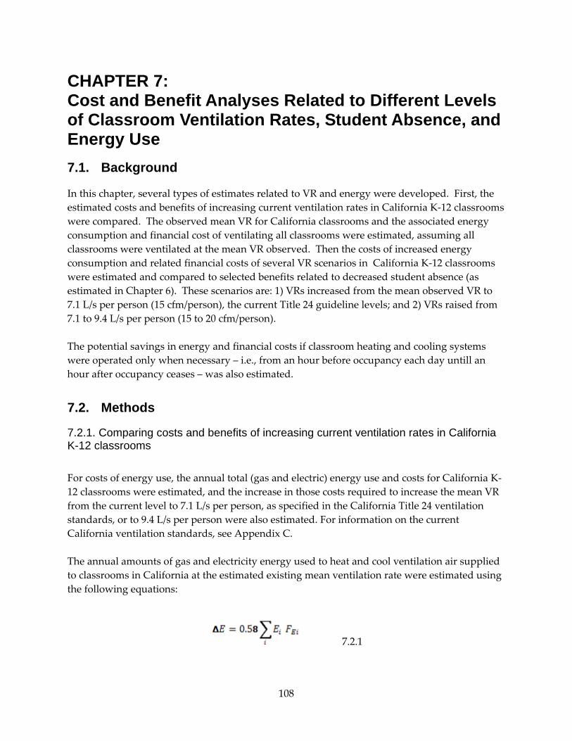
CHAPTER 7: Cost and Benefit Analyses Related to Different Levels of Classroom Ventilation Rates, Student Absence, and Energy Use 7.1. Background

In this chapter, several types of estimates related to VR and energy were developed. First, the estimated costs and benefits of increasing current ventilation rates in California K-12 classrooms were compared. The observed mean VR for California classrooms and the associated energy consumption and financial cost of ventilating all classrooms were estimated, assuming all classrooms were ventilated at the mean VR observed. Then the costs of increased energy consumption and related financial costs of several VR scenarios in California K-12 classrooms were estimated and compared to selected benefits related to decreased student absence (as estimated in Chapter 6). These scenarios are: 1) VRs increased from the mean observed VR to 7.1 L/s per person (15 cfm/person), the current Title 24 guideline levels; and 2) VRs raised from 7.1 to 9.4 L/s per person (15 to 20 cfm/person). The potential savings in energy and financial costs if classroom heating and cooling systems were operated only when necessary – i.e., from an hour before occupancy each day untill an hour after occupancy ceases – was also estimated.

7.2. Methods

7.2.1. Comparing costs and benefits of increasing current ventilation rates in California K-12 classrooms For costs of energy use, the annual total (gas and electric) energy use and costs for California K-12 classrooms were estimated, and the increase in those costs required to increase the mean VR from the current level to 7.1 L/s per person, as specified in the California Title 24 ventilation standards, or to 9.4 L/s per person were also estimated. For information on the current California ventilation standards, see Appendix C. The annual amounts of gas and electricity energy used to heat and cool ventilation air supplied to classrooms in California at the estimated existing mean ventilation rate were estimated using the following equations:

7.2.1

108

7.2.2

where ∆E is the electricity use for cooling and dehumidifying ventilation air, Ei is the total classroom electricity use for California climate zone i, ∆G is the gas use for heating ventilation air, Gi is the total classroom gas use for climate zone i, Fi and Gi are the fractional change in total classroom electricity and gas use, respectively, use for each 1 L/s per person change in ventilation rate in climate zone i, and V is the estimated mean ventilation rate of classrooms in California in L/s per person. Values of Ei and Gi were obtained from the California Energy Use Survey (http://capabilities.itron.com/ceusweb/) and exclude colleges and universities, but include all school floor area (41.4 x 106 m2), not just the area of classrooms. The coefficient of 0.58 is the ratio of classroom floor area to total floor area for California K-12 schools and yields estimates of energy use applicable to classrooms. The total classroom floor area was based on the product of the average classroom size (89 m2) and the estimated 268,000 classrooms (Whitmore et al. 2003). Values of FEi and FGi were based on energy simulations (Benne et al. 2009) for the stock of education buildings in U.S. Department of Energy (DOE) climate zones 4B and 4C. Values of F for DOE climate zone 4C were applied to California climate zones FCZ01, FCZ05, FCZ08, and FCZ13, and values of F for for DOE climate zone 4B were applied to the remaining California climate zones. Simulations show that the change in energy use with ventilation rate is approximately linear (Benne et al. 2009). Thus, values of FEi and FGi are not significantly coupled to the ventilation rate or the magnitude of change in ventilation rate. The calculation applies values of F determined for full schools to the classrooms that represent 58% of school floor area. The value of V was calculated from a steady mass balance equation relating V with equilibrium indoor carbon dioxide concentration:

7.2.3

where S is the carbon dioxide emission rate per student set equal to 0.0043 L/s (Haverinen-Shaughnessy et al. 2007), Cin is the equilibrium indoor carbon dioxide concentration and Cout is the outdoor carbon dioxide concentration. As an estimate of Cin, the mean value of the one-hour average highest indoor carbon dioxide concentration from the California Classroom survey (Whitmore et al. 2003) was used. This survey was designed to provide data representative of the California building stock; thus, the ventilation rates based on the California Classroom

109

Survey are likely to be more representative of the full stock of California classrooms than the ventilation rates obtained from the sample in the present study. The resulting estimated mean ventilation rate was 4.0 L/s per person. The same basic equations were used to estimate the increase in gas and electricity use expected if the mean classroom ventilation rates were increased from the estimated current mean value of 4.0 L/s per person to 7.1 L/s per person as specified in Title 24, or to 9.4 L/s per person. The associated annual gas and electricity costs were estimated by multiplying the energy use estimates by California-average gas and electricity prices for commercial building customers. The gas price was $0.028/kWh ($0.81 per therm) based on 2010 data from the Energy Information Agency (EIA), and the electricity price was $0.118/kWh based on data from December 2011 from the EIA. To estimate benefits of resulting decreased illness absence from increased ventilation rates, the methods and results presented in Chapter 6 were utilized 7.2.2. Estimating potential savings in energy and financial costs from heating and cooling classroom only when necessary Project objectives included developing estimates of the extent of unnecessary heating and cooling that takes place when classrooms are not occupied, and estimating the associated potential unnecessary energy use. The available data for estimating the extent of unnecessary heating and cooling were the classroom schedules and the measured indoor and outdoor air temperatures. The classroom schedules indicate when students are present in the classrooms. No information was available on the additional times when only the teachers occupied classrooms. Periods of heating and cooling during classroom occupancy by students were classified as periods of necessary heating and cooling. In addition, any heating or cooling during the one-hour periods before and after student occupancy were counted as periods of necessary heating and cooling given the substantial probability that teachers occupied the classrooms during these periods. A period prior to student attendance is also often employed to pre-heat or pre-cool the classroom before students arrive. Other periods of heating or cooling were classified as unnecessary; however, this characterization will result in some over-counting of unnecessary heating and cooling; for example, from periods when a teacher comes to work on a weekend and turns on the heating system. Indoor and outdoor temperature data provide an indication of the periods of heating and cooling. Signs of heating and cooling include the following:

1. An indoor temperature maintained in the comfort zone, e.g., 20 to 25 oC (68 to 77 oF) when it is substantially colder outdoors, e.g., less than 14 oC (57 oF) suggests heating.

110

2. Maintenance of the indoor temperature in the comfort zone, e.g., 20 to 25 oC (68 to 77 oF) when temperatures are higher outdoors than indoors suggests cooling.

3. An indoor temperature that does not follow the same time trend as the outdoor temperature (e.g., increase or decrease with time) suggests heating or cooling.

4. An indoor temperature that is maintained in the comfort zone and that cycles up and down within a few-degree range (typical of thermostatically-controlled systems) suggests heating or cooling.

Numerous factors complicate the analysis, leading to a substantial uncertainty in any estimation of the extent of unnecessary heating and cooling based on temperature data. For example, sunlight entering a window and operating lights and computers will heat a classroom when the heating system is turned off or reduce the need for heating when the system is operating. Also, the structure and content of classrooms absorb and release heat over time, causing time lags and dampening in indoor temperature trends relative to outdoor temperature trends. Classrooms vary in thermal mass (heat storage capacity), thermal insulation levels, heat release from lighting and computer equipment, and solar exposure. Manually controlled heating and cooling systems will not result in the same oscillation signal of thermostatically controlled systems. Errors in temperature measurements also cause uncertainties, considered small relative to the other sources of uncertainty. Some of these sources of uncertainty are diminished or eliminated during periods without occupancy; for example, there will be no manual control of heating or cooling, and rates of internal heat generation will generally be small, assuming that lights are off and computers are off or in sleep mode. Algorithms were developed to automatically detect periods of unnecessary heating and cooling based on the signs indicated in paragraphs 1 and 4 listed above. When the results of these algorithms were inspected graphically, it was clear that none was sufficiently reliable; however, an algorithm based on the signs described in paragraph 4 appeared promising. Consequently, to provide a rough estimation of the extent of unnecessary heating and cooling, plots of both indoor and outdoor temperature versus time for all classrooms were visually inspected during all times when students did not occupy the classrooms. A full year of data were inspected for each classroom. The one-hour periods before and after student occupancy were neglected for the reasons described above. When the signs described in paragraphs 1 – 4 were satisfied, unnecessary heating and cooling was assumed to occur and the associated time periods tabulated. The mean values of indoor and outdoor temperatures for each of these periods were also calculated. There is clearly a subjective element to the methodology used to define periods of unnecessary heating or cooling; however, the inspection-based procedure was judged more accurate than any fully automated algorithm that could be developed with the available resources. Figure 7.2.1 shows indoor and outdoor temperature data with an example of periods on two weekend days – between late morning and evening hours -- when the classroom was unoccupied but cooling was evident from the oscillations of indoor air temperature.

111

Figure 7.2.1: Example of cyclic oscillation in indoor air temperature data indicating space cooling, during two weekend days.

The unnecessary annual energy use associated with periods of unnecessary heating and cooling was roughly estimated. The calculations used simple energy models to account for heat transfer through the building envelope and heat gain or loss from outdoor air ventilation. The following equations were employed:

7.2.4

7.2.5

where:

EUH = the unnecessary annual energy used for heating in the sample of 168 classrooms

ε = efficiency of a gas heating system, assumed to equal 0.75

∆ti = the time elapsed during period “i” of unnecessary heating or cooling

U = the average overall thermal conductance (U value) of the classroom envelope

112

A = the classroom floor area

Tin = the average indoor temperature during period “i”

Tout = the average outdoor temperature during period “i”

H = the ceiling height, assumed to equal 3 m

N = the average air exchange rate of the classroom

ρ = the density of air at room temperature and atmospheric pressure equal to 1.2 kg m-3

CP = the specific heat of air at room temperature and atmospheric pressure equal to 1000 J kg-1 oC

EUC = the unnecessary annual energy used for space cooling in the sample of 168 classrooms

COPc = the coefficient of performance of the cooling system

COPH = the coefficient of performance of the electric heating system, when heating is electric

In these equations, the terms containing U values account for heating or cooling energy needed to overcome heat conduction through the envelope and the terms containing an N (air exchange rate) account for heating or cooling energy needed to heat or cool ventilation air. The equations assume negligible internal heat generation when the classrooms are unoccupied (e.g., lights and computers are off) and negligible solar heat gain, and do not account for heat storage in, or release from, the envelope or classroom contents. Also, the energy associated with dehumidification by air conditioning systems is neglected. Because classroom thermal and geometric characteristics were not collected, the calculations used an envelope U value of 0.5 W m-2 oC, typical of an insulated wall constructed with 2 x 4 wood framing; the mean floor area of 89 m2 from a survey of California classrooms (California Air Resources Board 2004); and an assumed ceiling height of 3 m. The floor area is multiplied by 1.8 to produce an estimate of the total area of the classroom envelope that connects to outdoors. This coefficient of 1.8 is based on the assumed ceiling height of 3 m, an assumed square floor (9.4 m by 9.4 m), and the assumption that the roof and, on-average, 2.5 walls connect to outdoors. Heat gain or loss through the classroom floor is neglected. For air exchange rate, the calculation used 1.3 h-1 , based on the average ventilation rate of 4 L/s per person in the California Classroom Survey as discussed previously, 25.3 students per classroom (from this study), and the classroom geometric characteristics described above. The coefficients of 0.7 and 0.3 are the fraction of gas and electricity used to heat California schools from the California Energy Use Survey (http://capabilities.itron.com/ceusweb/). A value of 3.2 was assumed for COPc corresponding to a Seasonal Energy Efficiency Ratio of approximately 12. A value of 2.2 was assumed for COPH corresponding to a Heating Seasonal Performance Factor of 7.7.

113

For the full set of California classrooms, the unnecessary heating and cooling energy for the sample of 168 classrooms was multiplied by the estimated 303,400 K-12 grade classrooms in California (http://www.cde.ca.gov/ls/fa/sf/facts.asp, accessed April 6, 2012) and divided by 168. To estimate gas and electricity costs, gas and electricity energy use estimates were multiplied by the respective California-average gas and electricity prices for commercial building customers. The gas price was $0.028/kWh ($0.81 per therm) based on 2010 data from the Energy Information Agency (EIA) and the electricity price was $0.118/kWh based on data from December 2011 from the EIA.

7.3. Results 7.3.1. Comparing costs and benefits of increasing current ventilation rates in California K-12 classrooms

7.3.1.1. Estimated costs of increasing current ventilation rate in California K-12 classrooms, Table 7.3.1 provides estimates of the annual energy used to heat and cool ventilation air supplied to California’s classrooms with the estimated mean existing ventilation rate of 4.0 L/s (8.5 cfm) per person. The incremental energy needed if mean ventilation rate was increased to 7.1 L/s (15 cfm) per person, as specified in Title 24, or to 9.4 L/s (20 cfm) per person, are also provided, along with estimated annual energy costs. For perspective, in parenthesis the energy consumed for ventilation is provided as a percentage of total building energy use. The calculations indicate that electricity used for ventilation in California classrooms is currently 1.5% of total classroom electricity use, while the gas used for ventilation is 5.2% of total classroom gas use. The associated annual energy costs are $3.5 million for electricity and $1.9 million for gas. Increasing the ventilation rate from 4.0 to 7.1 L/s (15 cfm) per person increases ventilation energy consumption and costs by 75%. Increasing the ventilation rate to 9.4 L/s (20 cfm) per person increases ventilation energy consumption and costs by 135%. All of the estimates are expected to have a high level of uncertainty. Ventilation rates in the existing stock of schools are estimated based on data from only 67 schools, with data collected only one day per classroom. Also, the model-based estimates of how ventilation rates affect school energy use have not been verified experimentally. One cannot directly measure the energy used for ventilation because this energy is just a portion of total energy consumption of the classrooms heating, ventilating, and air conditioning system.

114

Table 7.3.1: Estimates of the energy use and costs for cooling and heating the ventilation air provided to classrooms in California**, and potential benefits, at several ventilation rates.

Energy Use Costs Benefits

Electricity

(GWh)

{% of total}*

Gas

(GWh)

{% of total}^

Electricity Costs ($)

Gas Costs

($)

Total Increase

in Energy

Costs ($)

Increased State Revenue to School

Districts ($)

Reduced Care-giving by

Families ($)

At existing ventilation rate of 4.0 L/s per person

29

{1.5}

68

{5.2} 3.5 M 1.9 M 0 0 0

From increasing ventilation rate from 4.0 to 7.1 L/s per person

22 {1.2} 52

{4.3} 2.6 M 1.4 M 4.0 M 33 M 80 M

From increasing ventilation rate from 4.0 to 9.4 L/s per person

40

{2.1}

92

{7.6} 4.7 M 2.6 M 7.3 M 66 M 160 M

Abbreviations: M, million;

** 6,224,000 students in 9,900 schools in 2009-10 (from http://www.cde.ca.gov/ls/fa/sf/facts.asp, accessed March 15, 2012)

*percentage of total classroom electricity use

^percentage of total classroom gas use

115

7.3.1.2. Estimating benefits to school districts of decreased illness absence from increased ventilation rates in California K-12 classrooms Based on the analyses performed, and other available data, in Chapter 6 it was estimated that for the approximately 6,224,000 students in California K-12 schools (in 9,900 schools in 2009-10) (http://www.cde.ca.gov/ls/fa/sf/facts.asp, accessed April 6, 2012), an increase in mean VRs from 4 to 7.1 L/s per person, by decreasing illness absence, would increase annual state funding to school districts, under current formulas, by $33M (Table 7.3.1). Among this population, an increase in VR from 4 to 7.1 L/s per person would also produce benefits for families, from decreased costs for caregiver time, amounting to $80M. Total estimated benefits for this change in VRs equal $113M. A further increase from 7.1 to 9.4 L/s per person would increase annual state funding to school districts by an additional $33M, and increase benefits to families by an additional $880M, for an additional total benefit of $113M. Total benefits of increasing VRs from 4 to 7.1 L/s per person are estimated at $226M. Valuations of caregiver time include substantial subjectivity and uncertainty. The reduced costs in sick leave for teachers and staff, reductions in costs of medical care, or monetized improvements in quality of life for children were not estimated.

7.3.1.3. Comparing costs and benefits of increased ventilation rates in California K-12 classrooms In comparing these estimated benefits of increased VRs to the estimated costs (Table 7.3.1), either of the two specific types of benefits estimated for increased classroom VRs substantially outweighs the estimated energy costs. Total estimated benefits from an increase in VRs from 4.0 to 7.1 L/s per person are $113M, over 28 times the estimated costs of 4.0 M. Total benefits from an increase in VRs from 4.0 to 9.4 L/s per person, $226 million, are over 30 times the estimated additional energy costs of 7.3 M. There are also other potential benefits not considered here for increased VRs in classrooms. There are likely to be other financial costs not considered here, as well as some potential increased health effects and costs, such as from increased intake of and indoor exposures to pollutants from outdoors. If the magnitude of the relationships observed here, and the estimates of costs and benefits are confirmed, it would be advantageous to students, their families, and school districts, and highly cost effective, to insure that VRs in elementary school classrooms substantially exceed current recommended ventilation guidelines. Additional data and analyses would be necessary to refine these estimates of cost and benefit.

7.3.2. Estimating potential savings in energy and financial costs from heating and cooling classroom only when necessary Table 7.3.2 shows summary information from 168 classrooms. On average, unnecessary heating and cooling occurred for 32 and 13 hours per year per classroom, respectively; however, the extent of unnecessary cooling and heating varied greatly among classrooms; thus, the standard deviations were several times higher than the mean hours of heating of cooling. Of the classrooms, 21% had unnecessary heating and 22% had unnecessary cooling; however, 90% of

116

classrooms had 44 or fewer hours of unnecessary heating and 16 or fewer hours of unnecessary cooling. In a few classrooms, heating or cooling occurred during most of the unoccupied periods. In classrooms with unnecessary heating, on average this heating occurred 155 hours per year. In classrooms with unnecessary cooling, on average this cooling occurred 61 hours per year. The mean degree-hours of heating was almost four times larger than the mean degree-hours of cooling, because indoor-outdoor temperature differences are, on average, larger during the heating season.

Table 7.3.2: Summary information from analyses of periods of unnecessary heating and space cooling.

Parameter Mean Standard Deviation

Med-ian

Mini-

mum

90th

Percentile

Maxi-

mum

Fraction

>0* Mean >0**

Heating Hours 32 186 0 0 44 2,079 0.21 155

Cooling Hours 13 74 0 0 16 730 0.22 61

Heating Degree-Hours

(oC –h) 579 3,850 0 0 542 47,377 --- 2,777

Cooling Degree-Hours

(oC-h) 152 908 0 0 156 9,229 --- 691

*fraction of classrooms with unnecessary heating or cooling **mean value of parameter in classrooms with unnecessary heating or space cooling

Table 7.3.3 shows the estimates of energy consumption and energy costs for unnecessary heating and unnecessary space cooling, assuming the data from this study of three school districts are representative of the full set of grade K-12 schools in California. The estimated total energy costs for unnecessary heating and cooling are $1.5 million and $0.3 million, respectively, with a total cost of $1.8 million. The average annual cost per classroom is $6 for unnecessary heating and cooling. Total costs are highly influenced by substantial periods of unnecessary heating and cooling in a small fraction of all classrooms.

117

Table 7.3.3: Estimates statewide energy use and energy costs from unnecessary heating and cooling of grade K-12 classrooms.

Parameter Gas

(kWh per year)

Electricity

(kWh per year)

Gas

$ per year

Electricity

$ per year

Total

$ per year

Unnecessary Heating 3.3 x 107 4.8 x 106 9.1 x 105 5.6 x 105 1.5 x 106

Unnecessary Space Cooling -- 2.9 x 106 -- 3.4 x 105 3.4 x 105

Unnecessary Heating and

Space Cooling 3.3 x 107 7.7 x 106 9.1 x 105 9.0 x 105 1.8 x 106

7.4. Discussion 7.4.1 Comparing costs and benefits of increasing current ventilation rates in California K-12 classrooms

All three school districts, in the studied classrooms, had median daily VRs below the Title 24 minimum VR standard. Although providing classroom VRs below recommended levels in classrooms saves energy and money, the findings here suggest this strategy may have overriding but unrecognized costs of increased health problems and illness absence among students. The findings also suggest that increasing VRs above the recommended minimum levels, up to 20 L/s per person, may further substantially decrease illness absence. Total estimated benefits from an increase in VRs from 4.0 to 7.1 L/s per person are $113M, over 28 times the estimated costs of 4.0 M. Total benefits from an increase in VRs from 4.0 to 9.4 L/s per person, $226 million, are over 30 times the estimated additional energy costs of 7.3 M. Together, these findings suggest a potentially large opportunity to improve the health and attendance of elementary school students in California in a highly cost effective way, simply through provision of increased outdoor air ventilation in classrooms. These findings require replication and confirmation of causal connections. The school study on which these estimates are based had limitations. Problems with failure of the CO2 sensors, of inaccuracies in the CO2 data, and the difficulties of estimating true CO2 equilibrium levels, have been discussed in Chapter 6. These errors may have resulted in nonsystematic errors, or systematic overestimation of VRs, errors that are not likely to have created spurious relationships; instead, these errors may have reduced the apparent proportion of underventilated classrooms, underestimated true VR/illness absence relationships, and underestimated the range of VRs to which the findings apply. The estimates of energy costs, as already stated, are subject to substantial uncertainty. Nevertheless, very large errors would

118

have been necessary to create the magnitude of differences seen between the estimated costs and benefits. Implications

If the magnitude of the relationships observed, and the costs and benefits estimated are confirmed, it would be advantageous to students, their families, and school districts, and highly cost effective, to insure that VRs in elementary school classrooms substantially exceed current recommended ventilation guidelines. Additional data and analyses would be necessary to refine these estimates of cost and benefit, and to produce estimates for other climates. A more efficient alternative to general dilution of indoor pollutants by outside air ventilation is reduction in the emissions of indoor contaminants. To the extent that relationships of VR and illness absence in schools are mediated by infectious respiratory agents from occupants, this is not easily done. Improved particle filtration, however, would be helpful for reducing airborne infectious agents, and often less energy intensive than increased ventilation. The pattern of findings here, however, with ventilation in periods immediately prior to a day of illness absence not being more strongly related than longer prior periods, does not seem to point to infectious agents as the key driver of this relationship. If other indoor contaminants such as chemicals are important, for instance by causing increased susceptibility to infectious agents, then reducing emission of these contaminants or reducing their indoor concentrations with suitable air cleaning systems may be feasible in lieu of increasing VR. Research is necessary to identify the causal agents associated with the influence of VRs on illness absence.

7,4.2 Estimating potential savings in energy and financial costs from heating and cooling classroom only when necessary] The estimates of the energy consequences of unnecessary heating and cooling in classrooms have a high uncertainty due to the factors identified in the description of the methodology. However, the estimated total annual energy costs are a modest $1.8 million per year, or $6 per classroom. A large fraction of total costs are the result of long periods of unnecessary heating and cooling in a small fraction of classrooms. Thus, it would be most cost effective to identify and take corrective measures in this small subset of classrooms. Periods of unnecessary heating and cooling can be identified through analyses of indoor and outdoor air temperatures over time; however, further work is needed to automate the methods of analysis.

7.5. Conclusions The majority of the studied California elementary school classrooms in this study provided their students with less outdoor air ventilation than specified in current State guidelines, in some cases substantially less. If the magnitude of the relationships reported in Chapter 6, and the estimates of costs and benefit described in this chapter, are confirmed, it would be advantageous to students, their families, and school districts, and also highly cost effective

119

(with benefits exceeding costs by more than a factor of 25), to insure that VRs in elementary school classrooms not only meet but substantially exceed current recommended ventilation guidelines. An alternative strategy of reducing emission of indoor pollutants, or removing them by air cleaning, depending on which pollutants are responsible for increased illness absence with lower VRS, may provide many of the benefits of increased ventilation. The estimated total costs of energy used to condition unoccupied classrooms statewide is a modest $1.8 million, mostly for space heating. The average cost of wasted energy per classroom annually is under $10. Because a large fraction of the total costs are the result of long periods of unnecessary heating and cooling in a small fraction of classrooms, it would be most cost effective to identify and take corrective measures in this small set of classrooms.

120

REFERENCES Apte MG. 2006. A review of demand controlled ventilation. In: Healthy Buildings 2006.

Universidade de Porto, Portugal, 371-376. ASHRAE. 2007. ANSI/ASHRAE Standard 62.1. Ventilation for acceptable indoor air quality.

Atlanta, GA: American Society of Heating, Refrigerating, and Air Conditioning Engineers, Inc.

---. 2010. ANSI/ASHRAE Standard 62.1-2010: Ventilation for Acceptable Indoor Air Quality. Atlanta, GA, US: American Society of Heating, Refrigerating and Air-Conditioning Engineers, Inc.

ASTM. 1998. Standard guide for using indoor carbon dioxide concentrations to evaluate indoor air quality and ventilation. Designation D 6245-98. West Conshohocken, PA: American Society for Testing and Materials.

Bendrick GA. 1998. Seasonal variation of grounding rates among B-52H aircrew. Military Medicine 163:692-694.

Benne K, Griffith B, Long N, Torcellini P, Crawley D, Logee T. 2009. Assessment of the energy impacts of outside air in the commercial sector, NREL/TP-550-41955. Golden, CO: National Renewable Energy Laboratory.

Brandemuehl MJ, Braun JE. 1999. The impact of demand controlled and economizer ventilation strategies on energy use in buildings. ASHRAE Transactions 105(2):39-50.

Brundage JF, Scott RM, Lednar WM, Smith DW, Miller RN. 1988. Building-associated risk of febrile acute respiratory diseases in Army trainees. Jama 259(14):2108-2112.

California Air Resources Board. 2004. Report to the California Legislature: Environmental health conditions in California’s portable classrooms: California Air Resources Board and California Department of Health Services.

California Energy Commission. 2008. 2008 Building energy efficiency standards for residential and nonresidential buildings CEC-400-2008-001-CMF. Sacramento, CA: California Energy Commission.

Carpenter S, E. 1996. Energy and IAQ impacts of CO2-based demand controlled ventilation. ASHRAE Transactions 102(2):80-88.

Daisey JM, Angell WJ, Apte MG. 2003. Indoor Air Quality, ventilation and health symptoms in schools: an analysis of existing information. Indoor Air 13(1):53-64.

Deru M, Torcellini P. 2007. Source energy and emission factors for energy use in buildings, Technical report NREL/TP-550-38617. Golden, CO: National Renewable Eneregy Laboratory.

Eley Associates and New Building Institute. 2002. Utility cost forecasts: years 2005 through 2035. Jackson, Mississipi.

Emmerich SJ, Persily AK. 2001. State of the art review of CO2 demand controlled ventilation technology and application. NISTIR 6729. Gaithersburgh, MD: National Institute of Standards and Technology.

Erdmann CA, Apte MG. 2004. Mucous membrane and lower respiratory building related symptoms in relation to indoor carbon dioxide concentrations in the 100-building BASE dataset. Indoor Air 14(s8):127-134.

Fisk WJ, de Almeida AT. 1998. Sensor based demand controlled ventilation: a review. Energy and Buildings 29(1):35-44.

121

Fisk WJ, Faulkner D. 1992. Air exchange effectiveness in office buildings: measurement techniques and results. In: 1992 International Symposium on Room Air Convection and Ventilation Effectiveness. Tokyo:American Society of Heating, Refrigerating, and Air Conditioning Engineers, Inc., 213-223.

Fisk WJ, Faulkner D, Sullivan DP. 2006. Measuring outdoor airflow into HVAC systems. ASHRAE Journal 48(8):50-57.

---. 2007. A pilot study of the accuracy of CO2 sensors in commercial buildings. In: IAQ 2007 Healthy and Sustainable buildings. Baltimore, MD:ASHRAE.

Fisk WJ, Faulkner D, Sullivan DP, Bauman F. 1997. Air change effectiveness and pollutant removal efficiency during adverse mixing conditions. Indoor Air 7:55-63.

Fisk WJ, Faulkner D, Sullivan DP, Eliseeva E. 2009. CO2 monitoring for demand controlled ventilation in commercial buildings. LBNL-3279E. Berkeley, CA: Lawrence Berkeley National Laboratory.

Fisk WJ, Mirer AG, Mendell MJ. 2009. Quantitative relationship of sick building syndrome symptoms with ventilation rates. Indoor Air 19(2):159-165.

Fisk WJ, Sullivan DP. 2009. Optical people counting for demand controlled ventilation: a pilot study of counter performance, LBNL-3170E. Berkeley, CA: Lawrence Berkeley National Laboratory.

Fisk WJ, Sullivan DP, Faulkner D, Eliseeva E. 2010. CO2 monitoring for demand controlled ventilation in commercial buildings. LBNL-3279E. Berkeley, CA: Lawrence Berkeley National Laboratory.

Graham NM. 1990. The epidemiology of acute respiratory infections in children and adults: a global perspective. Epidemiologic reviews 12:149.

Haverinen-Shaughnessy U, Moschandreas DJ, Shaughnessy RJ. 2011. Association between substandard classroom ventilation rates and students' academic achievement. Indoor Air 21(2):121-131.

Haverinen-Shaughnessy U, Toivola M, Alm S, Putus T, Nevalainen A. 2007. Personal and microenvironmental concentrations of particles and microbial aerosol in relation to health symptoms among teachers. J Expo Sci Environ Epidemiol 17(2):182-190.

Hoge CW, Reichler MR, Dominguez EA, Bremer JC, Mastro TD, Hendricks KA, et al. 1994. An epidemic of pneumococcal disease in an overcrowded, inadequately ventilated jail. N Engl J Med 331(10):643-648.

Hong T, Fisk WJ. 2009. Assessment of energy savings potential from the use of demand control ventilation systems in general office spaces in California. LBNL-3165E. Berkeley, CA: Lawrence Berkeley National Laboratory.

Klepeis NE, Tsang AM, Behar JV. 1996. Analysis of the National Human Activity Pattern Survey (NHAPS) respondents from a standpoint of exposure assessment - Final EPA Report EPA/600/R-96/074. Washington, DC: U.S. EPA.

Lessler J, Reich NG, Brookmeyer R, Perl TM, Nelson KE, Cummings DAT. 2009. Incubation periods of acute respiratory viral infections: a systematic review. The Lancet infectious diseases 9(5):291-300.

Levy DE, Winickoff JP, Rigotti NA. 2011. School absenteeism among children living with smokers. Pediatrics 128(4):650-656.

Li Y, Leung GM, Tang JW, Yang X, Chao CYH, Lin JZ, et al. 2007. Role of ventilation in airborne transmission of infectious agents in the built environment - a multidisciplinary systematic review. Indoor Air 17(1):2-18.

122

Milton DK, Glencross PM, Walters MD. 2000. Risk of sick leave associated with outdoor air supply rate, humidification, and occupant complaints. Indoor Air 10(4):212-221.

Myatt TA, Staudenmayer J, Adams K, Walters M, Rudnick SN, Milton DK. 2002. A study of indoor carbon dioxide levels and sick leave among office workers. Environmental health: a global access science source 1.

National Buildings Controls Information Program. 2009. Product testing report, wall mounted carbon dioxide (CO2) transmitters. Ankeny, IA: Iowa Energy Center.

Nichol KL, Lind A, Margolis KL, Murdoch M, McFadden R, Hauge M, et al. 1995. The effectiveness of vaccination against influenza in healthy, working adults. New England Journal of Medicine 333(14):889-893.

Persily AK. 1997. Evaluating building IAQ and ventilation with carbon dioxide. ASHRAE Transactions 103(2):193-204.

Persily AK, Gorfain J. 2008. Analysis of ventilation data from the U.S. Environmental Protection Agency Building Assessment Survey and Evaluation (BASE) Study, NISTIR-7145-Revised. Bethesda. MD: National Institute for Standards and Technology.

Raatschen We. 1990. Demand controlled ventilating systems state of the aret review. Stockholm, Sweden: Swedish Council for Building Research.

Riley EC, Murphy G, Riley RL. 1978. Airborne spread of measles in a suburban elementary school. American Journal of Epidemiology 107(5):421-432.

Riley RL. 1982. Indoor airborne infection. Environment international 8(1):317-320. Rudnick SN, Milton DK. 2003. Risk of indoor airborne infection transmission estimated from

carbon dioxide concentration. Indoor air 13(3):237-245. Schell MB, Turner SC, Shim RO. 1998. Application of CO2-based demand controlled ventilation

using ASHRAE Standard 62: optimizing energy use and ventilation. ASHRAE Transactions 104(2):1213-1225.

Schmidt WP, Pebody R, Mangtani P. 2010. School absence data for influenza surveillance: a pilot study in the United Kingdom. Euro Surveill 15(3):19467.

Seppanen O, Fisk WJ, Lei QH. 2006. Ventilation and performance in office work. Indoor Air 16(1):28-36.

Seppanen O, Fisk WJ, Mendell MJ. 1999. Association of ventilation rates and CO2 concentrations with health and other responses in commercial and institutional buildings. Indoor Air 9(4):226-252.

Shaughnessy RJ, Haverinen-Shaughnessy U, Nevalainen A, Moschandreas D. 2006. A preliminary study on the association between ventilation rates in classrooms and student performance. Indoor Air 16(6):465-468.

Shendell DG, Prill R, Fisk WJ, Apte MG, Blake D, Faulkner D. 2004. Associations between classroom CO2 concentrations and student attendance in Washington and Idaho. Indoor Air 14(5):333-341.

Simoni M, Cai GH, Norback D, Annesi-Maesano I, Lavaud F, Sigsgaard T, et al. 2011. Total viable molds and fungal DNA in classrooms and association with respiratory health and pulmonary function of European schoolchildren. Pediatric Allergy and Immunology 22(8):843-852.

Steven Winters Associates. 2004. GSA LEED cost study:final report. Norwalk, Connecticut and Washington, DC.: Steven Winters Associates.

Sun Y, Wang Z, Zhang Y, Sundell J. 2011. In China, Students in Crowded Dormitories with a Low Ventilation Rate Have More Common Colds: Evidence for Airborne Transmission. PloS one 6(11):e27140.

123

Sundell J, Levin H, Nazaroff WW, Cain WS, Fisk WJ, Grimsrud DT, et al. 2011. Ventilation rates and health: multidisciplinary review of the scientific literature. Indoor Air 21(3):191-204.

Taylor Engineering. 2002. Demand controlled ventilation - measure analysis for Title 24-2005. Alameda, CA.

Torcellini P, Deru M, Griffith B, Benne K, Halverson M, Winiarski D, et al. 2008. DOE commercial building benchmark models. In: Proceedings of the 2008 ACEEE Summer Study on Energy Efficiency in Buildings. Asillomar, CA:American Council for an Energy Efficient Economy.

U.S. Energy Information Administration. 2003. 2003 Commercial building energy consumption survey. Washington, D. C. :Available: http://www.eia.doe.gov/emeu/cbecs/contents.html.

Wargocki P, Sundell J, Bischof W, Brundrett G, Fanger PO, Gyntelberg F, et al. 2002. Ventilation and health in non-industrial indoor environments: report from a European multidisciplinary scientific consensus meeting (EUROVEN). Indoor Air 12(2):113-128.

Wargocki P, Wyon DP. 2007. The effect of moderately raised classroom temperatures and classroom ventilation rate on the performance of schoolwork by children. HVAC&R Research 13(2):193-220.

Whitmore CA, Clayton A, Akland A. 2003. California Portable Classrooms Study, Phase II: Main Study, Final Report, Volume II. Research Triangle Park, NC: RTI International.

124

GLOSSARY

A the classroom floor area ABV absolute value AC air conditioned ADA actual daily attendance AVG average BA Bay Area Cal. Calibration CI confidence interval COPc coefficient of performance of the cooling system COPH coefficient of performance of the electric heating system, when heating is electric CV Central Valley CZ climate zone Cin mean value of the one-hour average highest indoor carbon dioxide concentration

from the California Classroom survey Cmax15 maximum 15-minute moving average classroom carbon dioxide concentration CO outside carbon dioxide concentration CP specific heat of air at room temperature and atmospheric pressure DCV demand controlled ventilation DDC direct digital control Ei total classroom electricity use for California climate zone i EUC unnecessary annual energy used for space cooling in the sample of 168 classrooms EUH unnecessary annual energy used for heating in the sample of 168 classrooms Fi the fractional change in total classroom electricity use for each 1 L/s per person

change in ventilation rate in climate zone i Gi total classroom gas use for climate zone i Gi fractional change in total classroom gas use use for each 1 L/s per person change in ventilation rate in climate zone i H ceiling height HVAC heating, ventilating, and air conditioning IA illness absence IRR incidence rate ratio Manu. manufacturer Max maximum Min minimum M1 manufacturer 1 M2 manufacturer 2 M3 manufacturer 3 M4 manufacturer 4

125

M5 manufacturer 5 M6 manufacturer 6 M7 manufacturer 7 M8 manufacturer 8 N carbon dioxide generation rate per person NPV net present value OA outdoor air PCS people counting system PV present value Ri revenue for student i RL revenue limit SC South Coast SD standard deviation Tin average indoor temperature during period i Tout average outdoor temperature during period i T1 type 1 T2 type 2 T3 type 3 T4 type 4 T5 type 5 U average overall thermal conductance of the classroom envelope V estimated mean ventilation rate of classrooms in California Vo outdoor air flow rate per person VR ventilation rate ZI zero inflation ZINB zero inflated negative binomial ∆E electricity use for cooling and dehumidifying ventilation air ∆G gas use for heating ventilation air ∆ti the time elapsed during period “i” of unnecessary heating or cooling ε efficiency of gas heating system ρ . density of air at room temperature and atmospheric pressure

126

APPENDIX A: Primary data from evaluation of accuracy of CO2 sensors Table A1. Data from multi-concentration calibration checks of sensor accuracy.

Build-ing Slope

Zero Offset (ppm)

Linear Fit R2

Error at 510 ppm (ppm)

Error at 760 ppm (ppm)

Error at 1010 ppm (ppm)

Manu-factur-er Code

Sen-sor Type

Self Cali-bra-tion

Sen-sor Age (yr))

-1 0.83 -55 0.99 -160 -196 -291 1 3 N NA -1 0.40 -113 0.68 -502 -756 -747 2 5 N NA -1 0.29 -77 0.76 -505 -717 -800 2 5 N NA -1 0.00 6 0.15 -502 -755 -1009 1 3 N NA -4 0.96 45 1.00 20 19 1 4 4 N 1 -4 0.93 49 1.00 18 -16 -2 4 4 N 1 -5 1.26 326 1.00 450 513 583 5 5 N 5 -5 1.01 -2 1.00 2 1 13 5 5 N 5 -5 1.14 -19 1.00 41 76 134 5 5 N 5 -6 0.96 31 1.00 10 -3 -11 4 1 Y 2 -6 0.91 45 1.00 7 -26 -44 4 1 Y 2 -6 1.08 -6 1.00 41 54 80 4 1 Y 2 -6 0.95 57 1.00 40 23 16 4 1 Y 2 -7 1.39 81 1.00 247 361 487 6 5 N 1 -7 0.91 39 1.00 -13 -26 -51 6 5 N 1 -8 0.93 21 1.00 -27 -30 -43 6 5 N 1 -9 0.97 18 1.00 -9 -1 -16 6 5 N 1 -9 0.87 56 1.00 -11 -48 -72 6 5 N 1 1 0.71 245 0.98 104 23 -99 4 4 N 0.5 1 0.69 195 0.99 53 -61 -135 4 4 N 0.5 1 0.79 60 0.99 -19 -126 -174 4 4 N 0.5 1 0.85 39 0.97 6 -81 -177 4 4 N 0.5 1 0.51 367 0.89 148 -19 -210 4 4 N 0.5 3 2.66 -534 1.00 319 697 1146 7 4 N 1 3 1.39 105 0.94 213 401 609 7 4 N 1 3 1.44 -119 0.99 152 157 284 7 4 N 1 3 1.50 -136 0.96 -507 180 399 7 4 N 1 3 1.52 -171 0.98 5 277 420 7 4 N 1 3 1.60 -237 0.91 95 467 7 4 N 1 4 0.98 44 1.00 24 38 19 7 4 N 5 4 0.87 38 0.99 -50 -58 -87 7 4 N 5 4 0.92 28 1.00 -22 -41 -38 7 4 N 5 4 0.90 -18 1.00 -64 -107 -91 7 4 N 5 4 0.94 35 1.00 -7 -6 -14 7 4 N 5 4 0.80 -139 1.00 -247 -300 -320 7 4 N 5 4 0.79 -173 1.00 -294 -324 -376 7 4 N 5

127

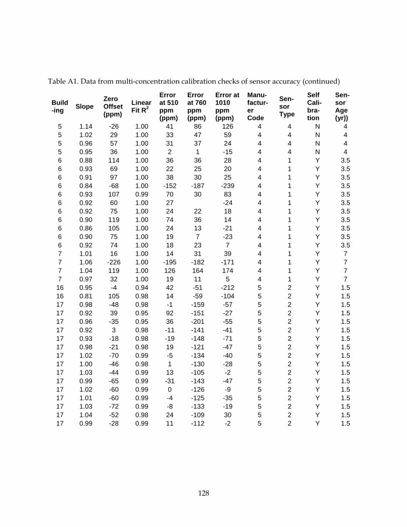
Table A1. Data from multi-concentration calibration checks of sensor accuracy (continued)

Build-ing Slope

Zero Offset (ppm)

Linear Fit R2

Error at 510 ppm (ppm)

Error at 760 ppm (ppm)

Error at 1010 ppm (ppm)

Manu-factur-er Code

Sen-sor Type

Self Cali-bra-tion

Sen-sor Age (yr))

5 1.14 -26 1.00 41 86 126 4 4 N 4 5 1.02 29 1.00 33 47 59 4 4 N 4 5 0.96 57 1.00 31 37 24 4 4 N 4 5 0.95 36 1.00 2 1 -15 4 4 N 4 6 0.88 114 1.00 36 36 28 4 1 Y 3.5 6 0.93 69 1.00 22 25 20 4 1 Y 3.5 6 0.91 97 1.00 38 30 25 4 1 Y 3.5 6 0.84 -68 1.00 -152 -187 -239 4 1 Y 3.5 6 0.93 107 0.99 70 30 83 4 1 Y 3.5 6 0.92 60 1.00 27 -24 4 1 Y 3.5 6 0.92 75 1.00 24 22 18 4 1 Y 3.5 6 0.90 119 1.00 74 36 14 4 1 Y 3.5 6 0.86 105 1.00 24 13 -21 4 1 Y 3.5 6 0.90 75 1.00 19 7 -23 4 1 Y 3.5 6 0.92 74 1.00 18 23 7 4 1 Y 3.5 7 1.01 16 1.00 14 31 39 4 1 Y 7 7 1.06 -226 1.00 -195 -182 -171 4 1 Y 7 7 1.04 119 1.00 126 164 174 4 1 Y 7 7 0.97 32 1.00 19 11 5 4 1 Y 7 16 0.95 -4 0.94 42 -51 -212 5 2 Y 1.5 16 0.81 105 0.98 14 -59 -104 5 2 Y 1.5 17 0.98 -48 0.98 -1 -159 -57 5 2 Y 1.5 17 0.92 39 0.95 92 -151 -27 5 2 Y 1.5 17 0.96 -35 0.95 36 -201 -55 5 2 Y 1.5 17 0.92 3 0.98 -11 -141 -41 5 2 Y 1.5 17 0.93 -18 0.98 -19 -148 -71 5 2 Y 1.5 17 0.98 -21 0.98 19 -121 -47 5 2 Y 1.5 17 1.02 -70 0.99 -5 -134 -40 5 2 Y 1.5 17 1.00 -46 0.98 1 -130 -28 5 2 Y 1.5 17 1.03 -44 0.99 13 -105 -2 5 2 Y 1.5 17 0.99 -65 0.99 -31 -143 -47 5 2 Y 1.5 17 1.02 -60 0.99 0 -126 -9 5 2 Y 1.5 17 1.01 -60 0.99 -4 -125 -35 5 2 Y 1.5 17 1.03 -72 0.99 -8 -133 -19 5 2 Y 1.5 17 1.04 -52 0.98 24 -109 30 5 2 Y 1.5 17 0.99 -28 0.99 11 -112 -2 5 2 Y 1.5

128

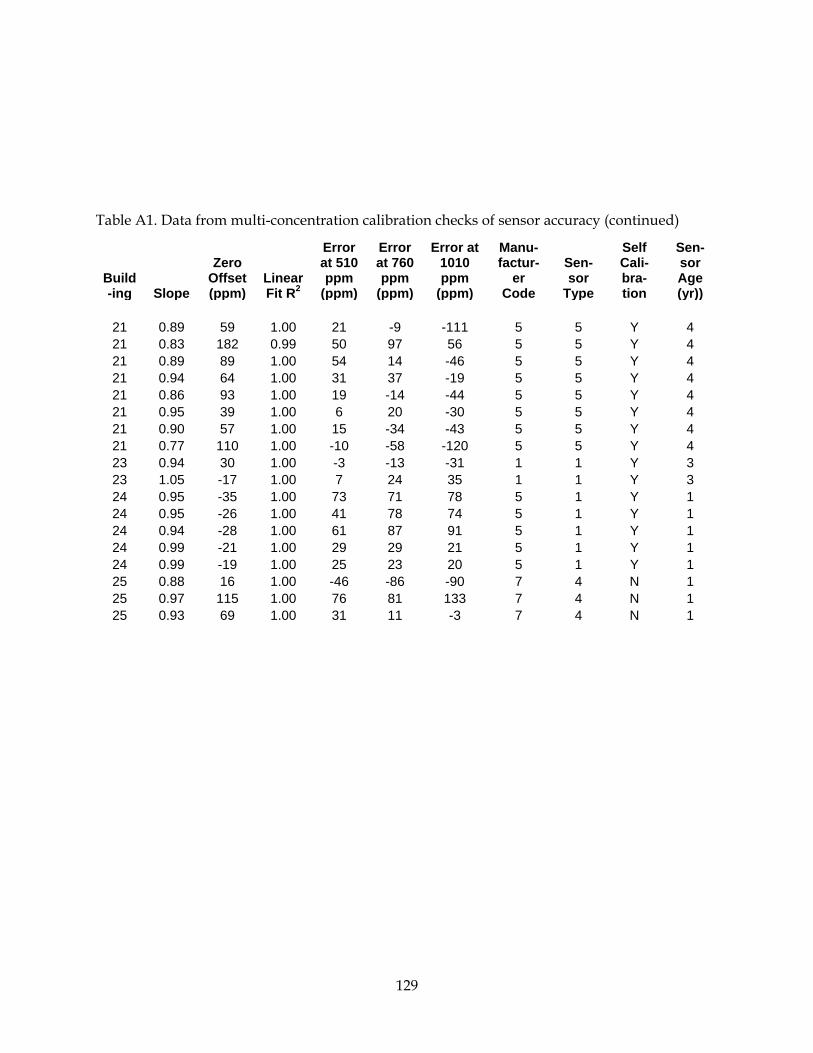
Table A1. Data from multi-concentration calibration checks of sensor accuracy (continued)

Build-ing Slope

Zero Offset (ppm)

Linear Fit R2

Error at 510 ppm

(ppm)

Error at 760 ppm

(ppm)

Error at 1010 ppm

(ppm)

Manu-factur-

er Code

Sen-sor

Type

Self Cali-bra-tion

Sen-sor Age (yr))

21 0.89 59 1.00 21 -9 -111 5 5 Y 4 21 0.83 182 0.99 50 97 56 5 5 Y 4 21 0.89 89 1.00 54 14 -46 5 5 Y 4 21 0.94 64 1.00 31 37 -19 5 5 Y 4 21 0.86 93 1.00 19 -14 -44 5 5 Y 4 21 0.95 39 1.00 6 20 -30 5 5 Y 4 21 0.90 57 1.00 15 -34 -43 5 5 Y 4 21 0.77 110 1.00 -10 -58 -120 5 5 Y 4 23 0.94 30 1.00 -3 -13 -31 1 1 Y 3 23 1.05 -17 1.00 7 24 35 1 1 Y 3 24 0.95 -35 1.00 73 71 78 5 1 Y 1 24 0.95 -26 1.00 41 78 74 5 1 Y 1 24 0.94 -28 1.00 61 87 91 5 1 Y 1 24 0.99 -21 1.00 29 29 21 5 1 Y 1 24 0.99 -19 1.00 25 23 20 5 1 Y 1 25 0.88 16 1.00 -46 -86 -90 7 4 N 1 25 0.97 115 1.00 76 81 133 7 4 N 1 25 0.93 69 1.00 31 11 -3 7 4 N 1

129

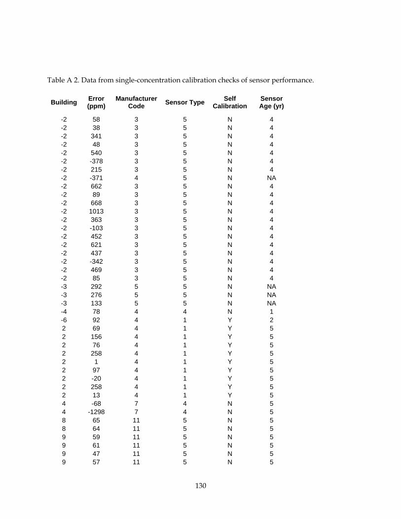
Table A 2. Data from single-concentration calibration checks of sensor performance.

Building Error (ppm)

Manufacturer Code Sensor Type Self

Calibration Sensor Age (yr)

-2 58 3 5 N 4 -2 38 3 5 N 4 -2 341 3 5 N 4 -2 48 3 5 N 4 -2 540 3 5 N 4 -2 -378 3 5 N 4 -2 215 3 5 N 4 -2 -371 4 5 N NA -2 662 3 5 N 4 -2 89 3 5 N 4 -2 668 3 5 N 4 -2 1013 3 5 N 4 -2 363 3 5 N 4 -2 -103 3 5 N 4 -2 452 3 5 N 4 -2 621 3 5 N 4 -2 437 3 5 N 4 -2 -342 3 5 N 4 -2 469 3 5 N 4 -2 85 3 5 N 4 -3 292 5 5 N NA -3 276 5 5 N NA -3 133 5 5 N NA -4 78 4 4 N 1 -6 92 4 1 Y 2 2 69 4 1 Y 5 2 156 4 1 Y 5 2 76 4 1 Y 5 2 258 4 1 Y 5 2 1 4 1 Y 5 2 97 4 1 Y 5 2 -20 4 1 Y 5 2 258 4 1 Y 5 2 13 4 1 Y 5 4 -68 7 4 N 5 4 -1298 7 4 N 5 8 65 11 5 N 5 8 64 11 5 N 5 9 59 11 5 N 5 9 61 11 5 N 5 9 47 11 5 N 5 9 57 11 5 N 5

130

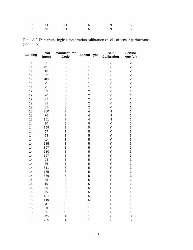
10 64 11 5 N 5 10 68 11 5 N 5

Table A 2. Data from single-concentration calibration checks of sensor performance. (continued).

Building Error (ppm)

Manufacturer Code Sensor Type Self

Calibration Sensor Age (yr)

11 35 5 1 Y 2 11 -310 5 1 Y 2 11 40 5 1 Y 2 11 33 5 1 Y 2 11 -80 5 1 Y 2 11 -1 5 1 Y 2 11 25 5 1 Y 2 12 33 5 2 Y 1 12 26 5 2 Y 1 12 37 5 2 Y 1 12 31 5 2 Y 1 12 65 5 2 Y 1 13 200 7 4 N 1 13 76 7 4 N 1 13 161 7 4 N 1 14 30 8 5 Y 3 14 858 8 5 Y 3 14 67 8 5 Y 3 14 98 8 5 Y 3 14 -14 8 5 Y 3 14 185 8 5 Y 3 14 307 8 5 Y 3 14 530 8 5 Y 3 14 197 8 5 Y 3 14 94 8 5 Y 3 14 86 8 5 Y 3 14 811 8 5 Y 3 14 185 8 5 Y 3 14 336 8 5 Y 3 15 35 9 5 Y 1 15 19 9 5 Y 1 15 30 9 5 Y 1 15 59 9 5 Y 1 15 131 9 5 Y 1 15 119 9 5 Y 1 15 -31 10 1 Y 1 15 -9 10 1 Y 1 18 95 10 1 Y 1 19 -25 4 1 Y 3 19 255 4 1 Y 3

131

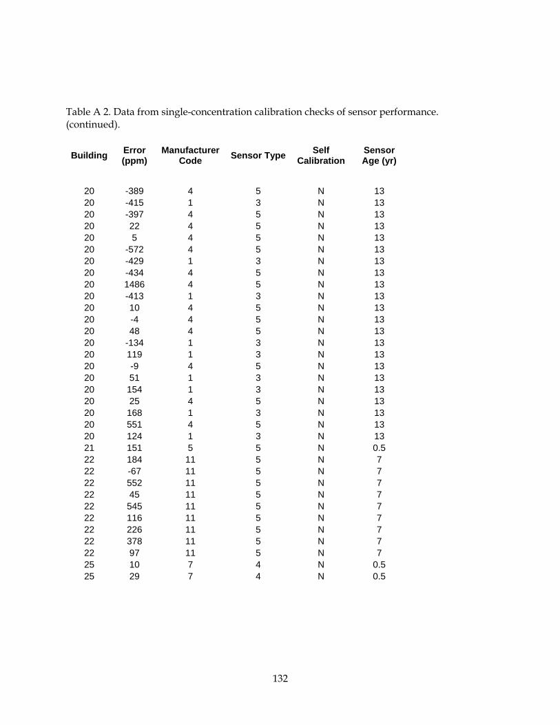
Table A 2. Data from single-concentration calibration checks of sensor performance. (continued).

Building Error (ppm)

Manufacturer Code Sensor Type Self

Calibration Sensor Age (yr)

20 -389 4 5 N 13 20 -415 1 3 N 13 20 -397 4 5 N 13 20 22 4 5 N 13 20 5 4 5 N 13 20 -572 4 5 N 13 20 -429 1 3 N 13 20 -434 4 5 N 13 20 1486 4 5 N 13 20 -413 1 3 N 13 20 10 4 5 N 13 20 -4 4 5 N 13 20 48 4 5 N 13 20 -134 1 3 N 13 20 119 1 3 N 13 20 -9 4 5 N 13 20 51 1 3 N 13 20 154 1 3 N 13 20 25 4 5 N 13 20 168 1 3 N 13 20 551 4 5 N 13 20 124 1 3 N 13 21 151 5 5 N 0.5 22 184 11 5 N 7 22 -67 11 5 N 7 22 552 11 5 N 7 22 45 11 5 N 7 22 545 11 5 N 7 22 116 11 5 N 7 22 226 11 5 N 7 22 378 11 5 N 7 22 97 11 5 N 7 25 10 7 4 N 0.5 25 29 7 4 N 0.5

132

APPENDIX B: Excerpts from specifications for demand controlled

ventilation in Title 24 and its appendices Section 121 – Requirements for Ventilation

All nonresidential, high-rise residential, and hotel/motel occupancies shall comply with the requirements of Section 121(a) through 121(e).

……

(a) General Requirements.

1. All enclosed spaces in a building that are normally used by humans

Required Demand Control Ventilation. HVAC systems with the following characteristics shall have demand ventilation controls complying with 121(c)4:

A. They have an air economizer; and

B. They serve a space with a design occupant density, or a maximum occupant load factor for egress purposes in the CBC, greater than or equal to 25 people per 1000 ft2 (40 square foot per person); and

C. They are either:

i. Single zone systems with any controls; or

ii. Multiple zone systems with Direct Digital Controls (DDC) to the zone level.

EXCEPTION 1 to Section 121(c)3: Classrooms, call centers, office spaces served by multiple zone systems that are continuously occupied during normal business hours with occupant density greater than 25 people per 1000 ft2 per Section 121(b)2B, healthcare facilities and medical buildings, and public areas of social services buildings are not required to have demand control ventilation.

EXCEPTION 2 to Section 121(c)3: Where space exhaust is greater than the design ventilation rate specified in Section 121(b)2B minus 0.2 cfm per ft2 of conditioned area.

EXCEPTION 3 to Section 121(c)3: Spaces that have processes or operations that generate dusts, fumes, mists, vapors, or gases and are not provided with local exhaust ventilation, such as indoor operation of internal combustion engines or areas designated for unvented food service preparation, or beauty salons shall not install demand control ventilation.

EXCEPTION 4 to Section 121(c)3: Spaces with an area of less than 150 square feet, or a design occupancy of less than 10 people per Section 121(b)2B.

4. Demand Control Ventilation Devices.

133

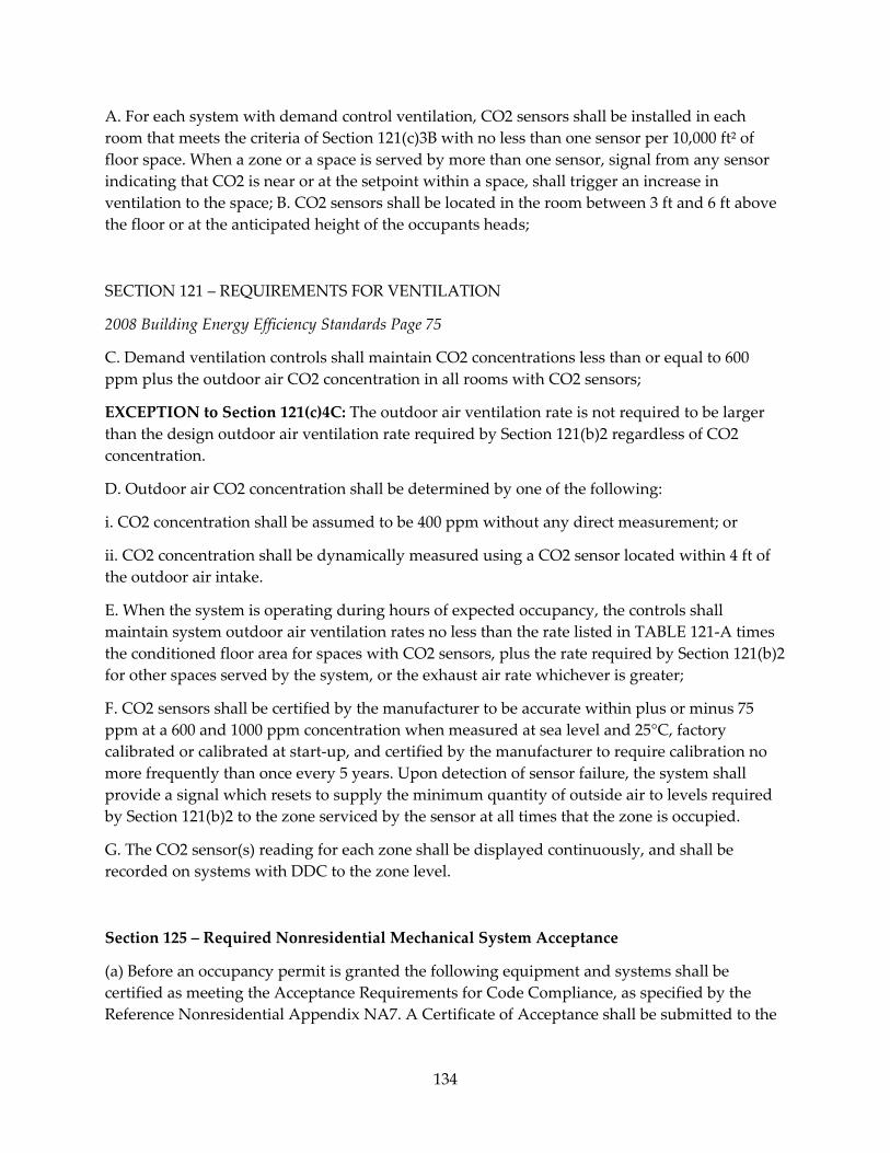
A. For each system with demand control ventilation, CO2 sensors shall be installed in each room that meets the criteria of Section 121(c)3B with no less than one sensor per 10,000 ft² of floor space. When a zone or a space is served by more than one sensor, signal from any sensor indicating that CO2 is near or at the setpoint within a space, shall trigger an increase in ventilation to the space; B. CO2 sensors shall be located in the room between 3 ft and 6 ft above the floor or at the anticipated height of the occupants heads;

SECTION 121 – REQUIREMENTS FOR VENTILATION

2008 Building Energy Efficiency Standards Page 75

C. Demand ventilation controls shall maintain CO2 concentrations less than or equal to 600 ppm plus the outdoor air CO2 concentration in all rooms with CO2 sensors;

EXCEPTION to Section 121(c)4C: The outdoor air ventilation rate is not required to be larger than the design outdoor air ventilation rate required by Section 121(b)2 regardless of CO2 concentration.

D. Outdoor air CO2 concentration shall be determined by one of the following:

i. CO2 concentration shall be assumed to be 400 ppm without any direct measurement; or

ii. CO2 concentration shall be dynamically measured using a CO2 sensor located within 4 ft of the outdoor air intake.

E. When the system is operating during hours of expected occupancy, the controls shall maintain system outdoor air ventilation rates no less than the rate listed in TABLE 121-A times the conditioned floor area for spaces with CO2 sensors, plus the rate required by Section 121(b)2 for other spaces served by the system, or the exhaust air rate whichever is greater;

F. CO2 sensors shall be certified by the manufacturer to be accurate within plus or minus 75 ppm at a 600 and 1000 ppm concentration when measured at sea level and 25°C, factory calibrated or calibrated at start-up, and certified by the manufacturer to require calibration no more frequently than once every 5 years. Upon detection of sensor failure, the system shall provide a signal which resets to supply the minimum quantity of outside air to levels required by Section 121(b)2 to the zone serviced by the sensor at all times that the zone is occupied.

G. The CO2 sensor(s) reading for each zone shall be displayed continuously, and shall be recorded on systems with DDC to the zone level.

Section 125 – Required Nonresidential Mechanical System Acceptance

(a) Before an occupancy permit is granted the following equipment and systems shall be certified as meeting the Acceptance Requirements for Code Compliance, as specified by the Reference Nonresidential Appendix NA7. A Certificate of Acceptance shall be submitted to the

134

enforcement agency that certifies that the equipment and systems meet the acceptance requirements:

……

5. Demand control ventilation systems required by Section 121(c)3 shall be tested in accordance with NA7.5.5

……

NA7.5.5 Demand Control Ventilation Systems

NA7.5.5.1 Construction Inspection

Prior to Functional Testing, verify and document the following:

• Carbon dioxide control sensor is factory calibrated or field-calibrated per §121(c)4.

• The sensor is located in the high density space between 3 ft and 6 ft above the floor or at the anticipated level of the occupants’ heads.

• demand controlled ventilation control setpoint is at or below the CO2 concentration permitted by §121(c)4C.

NA7.5.5.2 Functional Testing

Step 1: Disable economizer controls

Step 2: Simulate a signal at or slightly above the CO2 concentration setpoint required by §121(c)4C. Verify and document the following:

• For single zone units, outdoor air damper modulates open to satisfy the total ventilation air called for in the Certificate of Compliance.

• For multiple zone units, either outdoor air damper or zone damper modulate open to satisfy the zone ventilation requirements.

Step 3: Simulate signal well below the CO2 setpoint. Verify and document the following:

• For single zone units, outdoor air damper modulates to the design minimum value.

• For multiple zone units, either outdoor air damper or zone damper modulate to satisfy the reduced zone ventilation requirements.

Step 4: Restore economizer controls and remove all system overrides initiated during the test.

Step 5: With all controls restored, apply CO2 calibration gas at a concentration slightly above the setpoint to the sensor. Verify that the outdoor air damper modulates open to satisfy the total ventilation air called for in the Certificate of Compliance.

135

APPENDIX C: Current ventilation standards per State of California

and ASHRAE 2008 Building Energy Efficiency Standards

CALIFORNIA CODE OF REGULATIONS, TITLE 24, Part 6

SUBCHAPTER 3: SECTION 121 – REQUIREMENTS FOR VENTILATION, p. 73.

(b) Design Requirements for Minimum Quantities of Outdoor Air. Every space in a building shall be designed to have outdoor air ventilation according to Item 1 or 2 below:

1. Natural ventilation. A. Naturally ventilated spaces shall be permanently open to and within 20 feet of operable wall or roof openings to the outdoors, the openable area of which is not less than 5 percent of the conditioned floor area of the naturally ventilated space. Where openings are covered with louvers or otherwise obstructed, openable area shall be based on the free unobstructed area through the opening. . . .

2. Mechanical ventilation. Each space that is not naturally ventilated under Item 1 above shall be ventilated with a mechanical system capable of providing an outdoor air rate no less than the larger of: A. The conditioned floor area of the space times the applicable ventilation rate from TABLE 121-A (of 0.15 cfm/ft2); or B. 15 cfm per person times the expected number of occupants.

Source: http://www.energy.ca.gov/2008publications/CEC-400-2008-001/CEC-400-2008-001-CMF.PDF

Accessed April 14, 2012

Note: this California ventilation standard for classrooms is between the two default ASHRAE standards applicable to elementary school classrooms (Table A1-1.)

136

Table C-1. ASHRAE ventilation rate requirements (ASHRAE 2010, p. 12)

ASHRAE 62.1-2010

Space Use VR/person VR/area Overall, at specific assumed occupant density

Classrooms (ages 5-8)

5 L/s-person

(10 cfm/person)

0.6 L/s-m2

(0.12 cfm/ft2)

7.4 L/s per person*

{assumed 25 persons/100 m2}

(15 (14.8)cfm/person)*

{assumed 25 persons/1000 ft2}

Classrooms (ages 9+)

5 L/s-person

(10 cfm/person)

0.6 L/s-m2

(0.12 cfm/ft2)

6.7 L/s per person **

{assumed 35 persons/100 m2}

(13 (13.4) cfm/person)**

{assumed 35 persons/1000 ft2}

* assumed classroom occupant density =25 persons/100 m2 or /1,000 ft2

** assumed classroom occupant density = 35 persons/100 m2 or /1,000 ft2, but 100 m2 =1,076 ft2

(Note: Children in third grade are usually age 8 or 9 (but sometimes 7. Children in 4th and 5th grades will usually be ages 9+.)

137

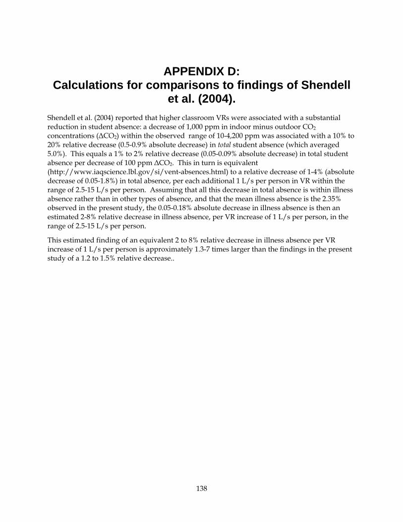
APPENDIX D: Calculations for comparisons to findings of Shendell

et al. (2004). Shendell et al. (2004) reported that higher classroom VRs were associated with a substantial reduction in student absence: a decrease of 1,000 ppm in indoor minus outdoor CO2 concentrations (ΔCO2) within the observed range of 10-4,200 ppm was associated with a 10% to 20% relative decrease (0.5-0.9% absolute decrease) in total student absence (which averaged 5.0%). This equals a 1% to 2% relative decrease (0.05-0.09% absolute decrease) in total student absence per decrease of 100 ppm ΔCO2. This in turn is equivalent (http://www.iaqscience.lbl.gov/si/vent-absences.html) to a relative decrease of 1-4% (absolute decrease of 0.05-1.8%) in total absence, per each additional 1 L/s per person in VR within the range of 2.5-15 L/s per person. Assuming that all this decrease in total absence is within illness absence rather than in other types of absence, and that the mean illness absence is the 2.35% observed in the present study, the 0.05-0.18% absolute decrease in illness absence is then an estimated 2-8% relative decrease in illness absence, per VR increase of 1 L/s per person, in the range of 2.5-15 L/s per person.

This estimated finding of an equivalent 2 to 8% relative decrease in illness absence per VR increase of 1 L/s per person is approximately 1.3-7 times larger than the findings in the present study of a 1.2 to 1.5% relative decrease..

138