Demand and routing models for urban goods movement …

European Transport \ Trasporti Europei n. 46 (2010): 3-23

3

Demand and routing models for urban goods

movement simulation

Antonio Polimeni 1∗∗∗∗, Francesco Russo

1, Antonino Vitetta

1

1 Mediterranea University of Reggio Calabria

Abstract

This paper presents a macro-architecture for simulating goods movements in an urban area. Urban

goods supply is analysed when the retailer is the decision-maker and chooses to supply his/her shop. Two

components are considered: demand in terms of goods supply and vehicle routing with constraints to

simulate goods movements.

To analyse demand we consider a multi-step model, while to analyse goods movements a Vehicle

Routing Problem with Time Windows (VRPTW) is formalized. We examine the distribution process for a

VRPTW in which the optimum paths between all the customers are combined to determine the best

vehicle trip chain. As regard optimum path search, a multipath approach is proposed that entails the

generation of more than one path between two delivery points. Some procedures (traffic assignment, real

time system measurement, reverse assignment) to estimate system performance are also proposed.

Finally, heuristics to solve the proposed problem are reported and their results are compared with those

exact.

Keywords: City Logistics; Goods movement; Vehicle routing problem.

1. Introduction

In this paper a macro-architecture to simulate goods movements in urban/metropolitan

areas is presented. Two components are considered: demand in terms of goods supply

and vehicle routing with constraints (time windows, fleet size, load factor …) to

simulate goods movements.

We consider a multi-step model, which on two different levels, gives as output: 1)

commodity flows, 2) vehicle flows. The first level is a commodity-based demand model

that simulates goods movements in terms of quantity: here we recall briefly a

commodity-based model, which simulates the quantity of goods purchased by a retailer.

The second simulates path choice made by the retailer. In this paper we report in detail

the Vehicle Routing Problem with Time Windows (VRPTW).

* Corresponding author: A. Polimeni ([email protected])


4

For the first level there are various models and methods to analyse urban goods

movements: the main classifications concern the output considered and the structure. As

regards the latter, some models have a structure similar to that used for passengers

(multi-step models), while others are based on the macro-economic approach (spatial

price equilibrium models) (Harker, 1985). In terms of output, while some models

estimate the commodity quantities transported, others estimate the vehicle number

involved in goods transport in urban areas (Ogden, 1992).

For the second level, as regards the Vehicle Routing Problem (VRP, it is a

combinatorial optimization problem), there is no single universally accepted definition

due to the diversity of constraints encountered in practice (Laporte, 2007).

In this paper, we consider the follow definition of the VRP: the problem consists in

determining a set of m vehicle routes starting and ending at the origin, and such that

each customer is visited by exactly one vehicle, the total demand of any route does not

exceed the vehicle capacity, and the total routing cost (time) is minimized (Laporte,

2007).

The VRP was introduced by Dantzig and Ramser (1959) so as to optimize the

movements of a fleet of gasoline delivery trucks. Since then research in this field has

greatly developed (recent works alone include Baker and Ayechew, 2003; Taniguchi et

al., 2007; Almeida et al., 2008; Wang an Lu, 2009; Jozefowiez et al., 2009).These

studies propose a formulation of the VRP (in an attempt to consider all the aspect of the

problem) and solution procedures (exact, heuristics). There are several types of VRP:

for example, referring to the customer may be termed a Dynamic VRP (DVRP), in

which the number of customers is a problem variable (Montemanni et al., 2005;

Hanshar and Ombuki-Berman, 2007); reference to the cost function can be termed the

Time-Dependent VRP (TDVRP) in which cost (travel time) is a function of travel day

(Malandraki and Daskin, 1992); referring to time constraints can be called the VRP with

Time Windows (VRPTW) in which deliveries can be made within a set time interval

(Hu et al., 2007; Ando and Taniguchi, 2006), and so on.

Several procedures have been proposed to solve the vehicle routing problems, both

exact (branch and bound, branch and cut) and heuristic procedures (tabù search, genetic

algorithms). For the exact approach, reference may be made to Fisher (1994), Toth and

Vigo (2002), and Baldacci et al. (2008). For the heuristic approach we may cite Laporte

(2007), Montemanni et al. (2005), Hanshar and Ombuki-Berman (2007), Laporte et al.

(2000), and Jones et al. (2002). Exact approaches have limitations in terms of

computing times and the size of the problems that can be solved. An extended review

concerning the VRP, several variants and solution approaches is reported in (Laporte,

2007; Gendreau et al., 2008).

The VRPTW proposed in this paper is treated as a combinatorial problem in which

the optimum paths between all the customers (Ben Akiva et al., 1984; Antonisse et al.,

1985; Cascetta et al., 1996; Russo and Vitetta, 2003) are combined to determine the best

vehicle trip chain.

In this paper a macro-architecture for goods movements is proposed (Russo and

Comi, 2010). The macro-architecture allows us to analyse the restocking process

starting from the delivery quantity and ending with the distribution process. In

particular, we analyse the distribution process for a VRPTW in which the optimum

paths between all the customers are combined to determine the best vehicle trip chain.

As regards the optimum path search, a multipath approach is proposed that concerns the

generation of more than one path between two delivery points. Moreover, some


5

procedures (traffic assignment, real time system measurement, reverse assignment) to

estimate system performance are proposed. Finally, some heuristics to solve the

proposed problem are reported and their results are compared with those exact.

The paper is organized as follows. In section 2 the macro-architecture is reported and

some aspects are developed in detail. In section 3 and 4 the routing models and the

algorithms are proposed. In section 5, the proposed algorithms are applied to some test

cases and a comparison between the results is reported. Finally, some conclusions are

drawn and future developments are outlined.

2. Macro-architecture methodology

The general macro-architecture of reference is that reported in the literature (Russo

and Comi, 2010; Russo and Comi, 2006; Russo et al., 2007). For the purposes of this

paper, analysis of the macro-architecture has four successive zooms, in which goods

movements are analysed from upper macro-levels (commodity and vehicle level) to the

path choice model (figure 1).

Figure 1: Macro-architecture of goods movements.

At the first zoom the goods quantity purchased in a zone by a retailer can be analysed

on two levels (Russo et al., 2007):

• commodity level, consisting of two macro-models:

� attraction macro-model for end-consumer quantities;

� acquisition macro-model for logistics trips from the retailer’s shop;

• vehicle level, which consists of two macro-models:

� service macro-model;

� path macro-model.


6

At the second zoom, we focus on the vehicle level. We obtain the service and the

time/path macro-models:

• the first (service) concerns the goods quantity delivered at each consignment and

the vehicles needed for restocking; in this model the distribution channels are

investigated (by distribution channel we mean how a product is physically

transferred or distributed from the production site to the point at which it is made

available to the customers), as is the service macro-model when the retailer can be

considered the decision-maker;

• the second concerns the time/path choice for each goods movement; the time/path

choice model simulates the time and path choice when the retailer moves from

his/her shop to one or more delivery points (the location of a wholesaler, a

producer, and so on).

At the third zoom, focusing on the time/path model, we find the time choice and path

choice models:

• the first simulates the time in which the goods must reach the retail shop; with this

model the departure time from the retail shop to reach the delivery points at an

established time window can also be simulated;

• the second concerns the path choice made by the retailer; this model can be

stochastic or deterministic (whether or not the costs are a random variable),

dynamic or static (whether or not the cost depends on time).

At the fourth zoom the One-to-One Problem (OOP) and the Vehicle Routing Problem

(VRP) are specified. Both problems can be tackled with a deterministic or probabilistic

approach, static or dynamic approach, depending on the approach to the path choice:

• the OOP concerns the case in which the retailer chooses to pick up goods at only

one delivery point;

• the VRP concerns the case in which restocking is done at various warehouse

points; we note that this problem is similar to the case in which a carrier restocks

several retailers from one warehouse.

In this paper we focus on the fourth zoom aggregation, with particular attention to the

VRP. The VRP is a combinatorial optimization problem: the minimum paths between

all possible pairs of delivery points are combined to find the best trip chains, where a

trip chain is a combination of several paths.

3. Routing models

The path choice model allows us to estimate the path choice probability/possibility for

the retailers in urban and metropolitan areas. As regards the problem of path simulation

and design for retail vehicles, two classes of individual users could be considered:

• private users (motorists and so on), i.e. those travelling for several reasons (work,

shopping, etc.) and following the path of maximum perceived utility;

• retailers, i.e. those travelling to restock their shops, who can be further

distinguished into:


7

� Non-Controlled (NC) retailers, i.e. those assumed to follow the path of

maximum perceived utility in the same way as private users (in accordance

with User Equilibrium-UE hypothesis);

� Controlled (C) retailers, i.e. those obtaining indications supplied by an

external (or internal) authority regarding optimal paths (that satisfy specific

criteria, e.g. time minimization) to follow, who are assumed, rather than to

maximize their own utility, to cooperate in minimizing total internal costs (in

accordance with system optimum-SO hypothesis).

Moreover, it is assumed that the number of C-retailers is smaller than the sum of

private users and NC-retailers. In a city, the number of private users is at least 100 times

greater than that of the retailers present. In such conditions the C-retailer’s path choice

behaviour does not affect system performance (i.e. link/path costs). The behaviour of

independent users and NC-retailers can be simulated in accordance with UE hypothesis

to obtain the costs on the network (possibly as a function of flows, assuming that the

network is congested and that the system is dynamic). Taking account of network costs,

the optimal path according to SO hypothesis for C-retailers can be designed considering

the network costs derived from UE.

The proposed procedure can be summarized in three steps.

STEP 1 - System performance estimation. In this step, the transport system is analysed

in order to estimate system performance (i.e. in terms of travel time or travel cost). This

objective can be achieved through static or dynamic Traffic Assignment (TA), Real-

time System Monitoring (RSM) or Reverse Assignment (RA) (Russo and Vitetta,

2005).

STEP 2 - One-to-One Problem (OOP) solution. In this step, the shortest path between

each delivery point pair is calculated, taking account of the costs obtained by step 1; the

mono–path and multi–path approach (MOOP) can be considered:

• in the mono-path case, with a deterministic approach, just one path (equal to the

shortest path) with maximum choice probability (equal to 1) is generated; this

approach, extensively used in the literature, is not very realistic due to the fact that

it does not take into account the uncertainty related to the simulation of user

perception of the alternative and the variability of the system states in time, hence

its dynamic nature;

• in the multi-path case (Multi-path OOP, MOOP), with a probabilistic approach, a

set of possible paths is generated, each of which has a choice

possibility/probability that depends on the user perception of the alternative and

the possibility/probability of there being a specific system state that influences the

choice process.

STEP 3 - VRP solution. To solve the VRP, the OOP solution obtained at step 2 is

considered. The objective is to calculate the best combination of shortest paths in order

to visit a succession of customers in the least time/cost possible whilst respecting some

constraints. If the one-to-one problem is solved using a multi-path approach, we have a

multi-path VRP (MVRP).


8

In figure 2 we report the three simulation steps for the case in which the multi-path

approach is used. In step 1 the data input are the supply and demand. Using TA, RSM

and/or RA it is possible to obtain cost and flow for each link. In the general case

(dynamic case) the cost and flow are time-dependent. The costs and flows found at step

1 are the input for step 2 which, in a multi-path approach, give the probability of

choosing paths belonging to a set of possible paths. The path choice probability is the

input for step 3, where the VRP is solved (using an appropriate procedure) to obtain the

trip chains.

Figure 2: Solving the restocking problem.

Below (sub-sections 3.1, 3.2 and 3.3) steps 1, 2 and 3 are itemized.

The following notations are used:

N = {1, 2, …, n}, node set;

L = {a : a = (i,j) ∀ i, j ∈N}, link set;

Z = {1, 2, …, m}, Z ⊂ N nodes must be visited;

f link flow vector with component fa on link a∈L;

h path flow vector with component hk on path k;

c link cost vector with component ca on link a;

g path cost vector with component gk on path k;

gADD

is the additive path cost vector; an element gkADD

is defined as the sum of the

links belonging to path k;

gNA

is the non-additive path cost vector;

u is the retailer’s shop;

NV ={1, 2, …, NVmax}, set of goods vehicles;

bj vehicle capacity, j=1, 2, …, NVmax;

Qj vehicle load, j=1, 2, …, NVmax;

ri demand on node i;

BTl,k penalty before time at client (node) l using path k;


9

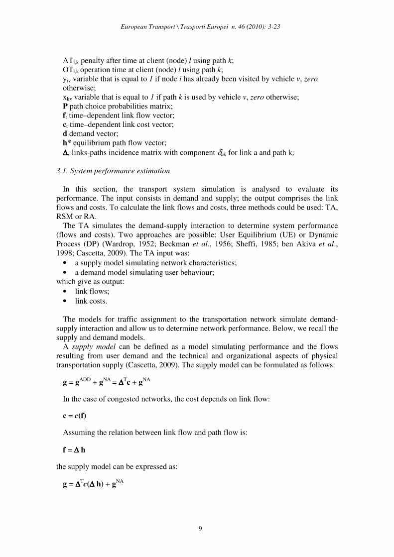
ATl,k penalty after time at client (node) l using path k;

OTl,k operation time at client (node) l using path k;

yiv variable that is equal to 1 if node i has already been visited by vehicle v, zero

otherwise;

xkv variable that is equal to 1 if path k is used by vehicle v, zero otherwise;

P path choice probabilities matrix;

ft time–dependent link flow vector;

ct time–dependent link cost vector;

d demand vector;

h* equilibrium path flow vector;

∆∆∆∆, links-paths incidence matrix with component δak for link a and path k;

3.1. System performance estimation

In this section, the transport system simulation is analysed to evaluate its

performance. The input consists in demand and supply; the output comprises the link

flows and costs. To calculate the link flows and costs, three methods could be used: TA,

RSM or RA.

The TA simulates the demand-supply interaction to determine system performance

(flows and costs). Two approaches are possible: User Equilibrium (UE) or Dynamic

Process (DP) (Wardrop, 1952; Beckman et al., 1956; Sheffi, 1985; ben Akiva et al.,

1998; Cascetta, 2009). The TA input was:

• a supply model simulating network characteristics;

• a demand model simulating user behaviour;

which give as output:

• link flows;

• link costs.

The models for traffic assignment to the transportation network simulate demand-

supply interaction and allow us to determine network performance. Below, we recall the

supply and demand models.

A supply model can be defined as a model simulating performance and the flows

resulting from user demand and the technical and organizational aspects of physical

transportation supply (Cascetta, 2009). The supply model can be formulated as follows:

g = gADD

+ gNA

= ∆∆∆∆Tc + g

NA

In the case of congested networks, the cost depends on link flow:

c = c(f)

Assuming the relation between link flow and path flow is:

f = ∆ ∆ ∆ ∆ h

the supply model can be expressed as:

g = ∆ ∆ ∆ ∆Tc(∆ ∆ ∆ ∆ h) + g

NA


10

A demand model can be defined as a mathematical relationship between demand

flows and the transportation supply system (Cascetta, 2009). The demand model may be

formulated as follows:

h = P(-g) d

The TA model is obtained by combining the supply model and demand model. The

TA can be solved with a static or dynamic approach; static assignment models simulate

a transportation system in stationary conditions, reproducing the condition in which link

flows and link costs are mutually consistent. The output is the link flow vector f and the

link cost vector c(f). To calculate the link flow a Stochastic User Equilibrium (SUE) is

considered; the SUE requires an algorithm to solve the fixed point model: the applied

algorithm is based on the Method of Successive Averages (MSA).

Equilibrium link flows (deterministic or stochastic) can be expressed as the solution

of a fixed-point model (Cascetta, 2009):

f*= ∆∆∆∆ P(-∆∆∆∆Tc(∆∆∆∆h*) - g

NA) d

Dynamic traffic assignment models remove the assumptions of static models,

allowing transportation system evolution to be represented. Dynamic traffic assignment

models can be analysed in relation to the characteristics of the link model adopted. In

particular, link flow representation can be continuous or discrete, and cost functions can

be aggregate or disaggregate. The output is the link flow vector for each time t, ft, and

the link cost vector, ct(ft).

The RSM allows us to obtain the traffic flow data using monitoring techniques and

can be obtained with:

• measurement at fixed points in the network with traditional measurement systems

like loop detectors and image processing (Hoose, 1991);

• floating cars (Torday and Dumont, 2004) in the network (individual cars, taxis,

transit system vehicles).

RSM costs and flows are usually made for a subset S ⊆ L of the network links. For

each link a ∈ S RSM provides the link flow vector fRSM and the link cost vector cRSM

and/or the link flow vector for each time t ft,RSM and the link cost vector ct,RSM. Because

the values are available only in a subset of links, RSM has to be used together with TA,

giving RA models. RA models (Russo and Vitetta, 2005) have the following input:

• link flows;

• link performance in terms of costs;

and give as output

• the link cost parameters of the cost-flow functions used in the supply model;

• the value (number of trips) and/or the model parameters of the demand model.

RA models, starting from observed costs and flows (i.e. provided by RSM), provide

the demand value and/or parameter and/or the link cost parameters of the cost-flow

functions used in the supply model. Hence, RA can be formulated as an optimum

problem which, starting from d, fRSM and cRSM, provides f*RSM and c*RSM in the


11

whole network. In the time-dependent problem the outputs are f*t,RSM and c*t,RSM

(Russo and Vitetta, 2005).

3.2. One-to-One Problem

As input the OOP has costs and flows and, as output, it supplies the optimal paths; the

users involved are C-retailers. In this paper, we consider C-retailer path choice using

two approaches:

• the mono-path approach;

• the multi-path approach, which can be mono-criterion or multi-criteria.

The mono-path concerns the generation of only one path between an origin and a

destination. This approach, widely used in the literature, is deterministic and the path

generated is assumed the best path. Hence, the output is a path set ΓΓΓΓ. An element

k∈ Γ Γ Γ Γ is associated to each origin/destination pair.

The MOOP concerns the generation of more than one path between an origin and a

destination. This approach is probabilistic; the link cost is a random variable, which

means:

• each path has a probability to come;

• the retailer is ill-informed on the system state.

For each retailer n the output consists of some path sets ΓΓΓΓin; each path k∈ Γ Γ Γ Γi

n has a

probability pn(k); an element k∈ Γ Γ Γ Γi

n is associated to each pair of delivery points.

In the literature, only the mono-path approach is used, but it is plain that in reality the

multi-path approach should be used since it takes into account the uncertainty related to

simulating the user perception of the alternative and system state variability over time,

hence its dynamic nature (Russo and Vitetta, 2006).

In the MOOP a choice set is generated; in this phase we distinguish:

• formation, concerning the structure of the potential analytical path set/sets;

• extraction, concerning the extraction of the choice set.

In this paper, to solve the OOP, a probabilistic approach is adopted. In this approach,

having established a criterion to define the cost (e.g. minimum travel time), the link

cost, and hence the path cost, is a random variable resulting from the retailer’s

perception of the possible alternatives (paths). The probability pn(k) can be calculated

as the sum, on all the sub-sets ΓΓΓΓi which contain the alternative k, of the product between

the probability pn( ΓΓΓΓi

n) of the sub-set ΓΓΓΓi

n and the conditional probability pn(k/ΓΓΓΓi

n ) of

choosing path k given the choice set ΓΓΓΓin (Manski, 1977):

pn(k) = Σi p

n(ΓΓΓΓi

n) pn (k/ΓΓΓΓi

n)

To calculate the paths, a modification of the Dijkstra algorithm is used in order to

evaluate more than one path between an origin and a destination (Russo and Vitetta,

2006).


12

3.3. Vehicle Routing Problem

The vehicle routing problem is introduced to simulate the restocking approach when

the retailer chooses to restock in some delivery points: the problem can be described as

the design of optimal trip chains from the retail shop to a set of delivery points

(warehouses, producers,…); each point can be reached exactly once. The constraints are

economic (travel cost, operation costs …) and operational (vehicle capacity, time

windows,…). The objective is to purchase whilst respecting the constraints and

minimizing the total cost.

As input, the VRP has paths generated by the OOP. As output, it supplies the optimal

trip chains that join the delivery points (a trip chain is a combination of several paths).

If the OOP is tackled with the mono-path approach the solution is a set Ψ Ψ Ψ Ψ of trip

chains. If the OOP is tackled with the multi-path approach, it is possible to formulate an

MVRP. For each retailer n, the output consists of trip chain sets ΨΨΨΨin; each trip chain

κ∈ Γ Γ Γ Γin may be linked to a probability p

n(κ). Moreover, the MVRP can be static or

dynamic: in the first case we have c(f) as input variable, in the second case ct(ft).

The problem constraints are as follows:

• a delivery point can be reached exactly once;

• vehicle capacity;

• time windows.

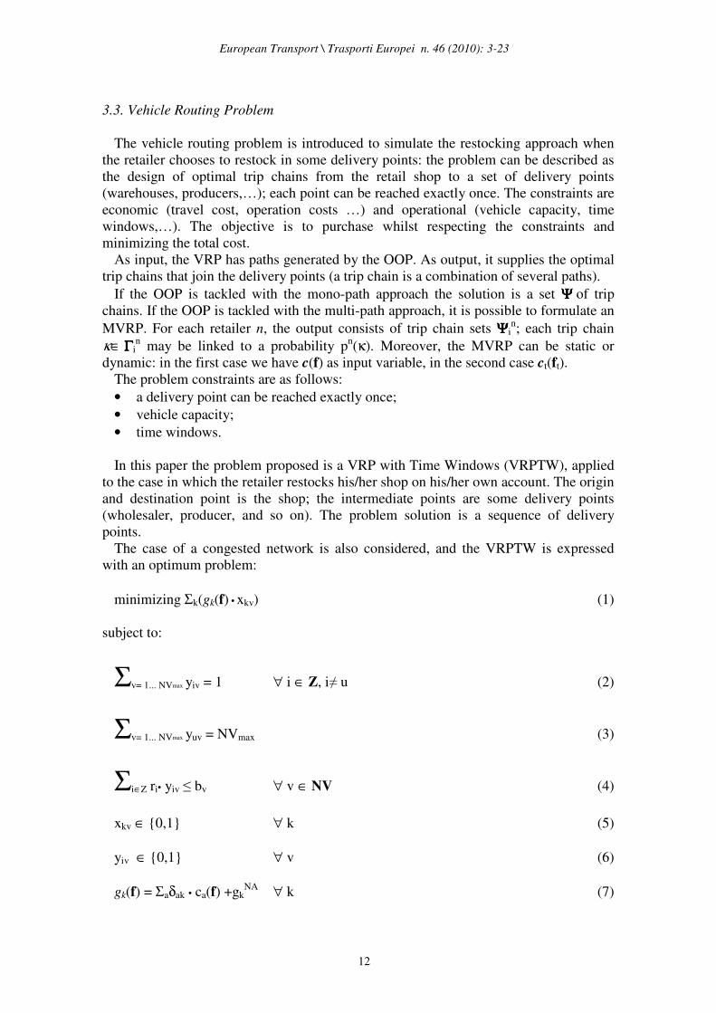
In this paper the problem proposed is a VRP with Time Windows (VRPTW), applied

to the case in which the retailer restocks his/her shop on his/her own account. The origin

and destination point is the shop; the intermediate points are some delivery points

(wholesaler, producer, and so on). The problem solution is a sequence of delivery

points.

The case of a congested network is also considered, and the VRPTW is expressed

with an optimum problem:

minimizing Σk(gk(f) • xkv) (1)

subject to:

Σv= 1... NVmax yiv = 1 ∀ i ∈ Z, i≠ u (2)

Σv= 1... NVmax yuv = NVmax (3)

Σi∈Z ri• yiv ≤ bv ∀ v ∈ NV (4)

xkv ∈ {0,1} ∀ k (5)

yiv ∈ {0,1} ∀ v (6)

gk(f) = Σaδak • ca(f) +gkNA

∀ k (7)


13

Constraint 2 indicates that a node can be visited exactly once, constraint 3 that all

vehicles go back to the shop. In the case in which we have a single vehicle, constraints 2

and 3 degenerate into:

yi = 1 ∀ i ∈ Z, i≠ u

yu = 1

Constraint 4 is a capacity constraint. In the case of a single vehicle:

Σi∈Z ri• yi ≤ b

Constraint 5 indicates that the problem variable can only take the value zero or one, in

the case of a single vehicle:

xk ∈ {0,1} ∀ k

In constraint 7, the term gk(f) is the path cost between an origin/destination pair (shop

– delivery point, delivery point – delivery point, delivery point – shop). The path cost is

the sum of two elements: additive costs, which depend on link and flow characteristics,

and non-additive costs. The first element is obtained by solving an OOP, using a

shortest path search procedure. Assuming that the travel time on the path is the path

cost, a cost matrix may be defined, in which the generic element is the travel time

between an origin/destination pair. The second element consists of three components:

the before-time (BTl,k), after-time (ATl,k) and operation time (OTl,k) for client l visited

by path k. These components are calculated for each client reached by the vehicle v that

follows the path considered.

Before-time indicates the time penalty for advance arrival at the node. It is assumed

that before-time is a linear function of arrival time. After-time indicates the time penalty

for delayed arrival at the node. It is assumed that if the vehicle arrives late the penalty is

a fixed value. Operation time indicates the time for unloading operations. Operation

time is a function of goods quantity delivered at the delivery point l:

OTl=m • ql

in which

m is the proportionality factor;

ql is the quantity of goods delivered to delivery point l.

The non-additive path cost can then be formalized as:

gkNA

= Σl(BTl,k + ATl,k + OTl,k)

Finally, xkv is the problem variable. It is a binary variable that is equal to one if path k

is used by vehicle v, zero otherwise. Note that the proposed formulation is independent


14

of vehicle type and that the time penalties (before-time and after time) allow us to

obtain a solution that respects the time windows.

To solve the problem expressed by equation (1) exact (e.g. Branch and Bound),

heuristic procedures (i.e. simulated annealing, genetic algorithms, other heuristic) or

hybrid procedures can be used. In this paper a greedy procedure and a genetic algorithm

are proposed; the results obtained are compared with those exact. In the next section the

above algorithms are itemized.

4. Routing algorithms

A retailer who restocks his/her shop on his/her own account in most cases makes a

small number of stops. In this case it is acceptable to use an exact algorithm to solve the

problem (for example Branch and Bound or an exhaustive evaluation approach).

However, if the node number increases the computing times, it is necessary to use a

heuristic procedure.

In this section we report:

• a greedy algorithm (called Iterated Nearest Insertion, INI);

• a Genetic Algorithm (GA).

4.1. Iterated Nearest Insertion Algorithm

The Iterated Nearest Insertion (INI) algorithm is a greedy algorithm that consists in an

insertion of nodes (delivery points) to minimize the travel time. At each successive

insertion the delivery point nearest the previous one is inserted into the solution. When a

solution is found, the procedure is repeated l times, with l greater than 1 and less than

the number of delivery points. A single iteration of the algorithm is schematized as

follows.

STEP 0 Initialize. The node list W comprises the delivery points and the point where the

retailer is located. The current node is the point where the retailer is located.

STEP 1 List. The current node is deleted from W.

STEP 2 Path. The shortest paths between the current node and the delivery points in W

are calculated.

STEP 3 Update. The nearest delivery point is the new current node.

STEP 4 Repeat. Go to step 1 while W≠ ∅.

4.2. Genetic Algorithm

In this paper, we also propose a genetic algorithm (GA) to solve the problem (1).

Problem solution is a node sequence (delivery points) associated to individual vehicles.

The following definitions are adopted:

• trip chain: an ordered sequence of delivery points associated to one vehicle

κj=(u…, i, …u) ∀ i ∈ Z. Each trip chain has the depot u as the initial and final

node;

• solution: a set of trip chains ΨΨΨΨ={(κ1,κ2,…,κj,…) j=1,2,…, NVmax}. A solution has

as many trip chains as there are vehicles.


15

If we have a single vehicle, the solution coincides with the trip chain. The genetic

algorithm proposed is reported in figure 3 and its steps are analysed below. Note that the

procedure is applicable whether we have a single vehicle or we have more than one.

The initial population consists of a fixed number of solutions (population size). To

each solution a cost value is associated.

Figure 3: Genetic algorithm.

In the first step the initial population is determined; the procedure used being a

heuristic insertion procedure in which the trip chain is built with the iterative insertion

of nodes, respecting vehicle capacity. The procedure is formulated as follows:

Maximizing Qv = Σi∈Z δiqi,v

subject to:

Qv ≤ b

in which

δi is a binary variable that is equal to 1 if node i can be added to the trip chain

associated to vehicle v, zero otherwise;

qi,v is the goods quantity at node i delivered by vehicle v.

For each trip chain belonging to a solution, the first node is inserted randomly; the trip

chain is completed by random insertion of nodes, maximizing function Qv. At the first

iteration, the parent population and initial population coincide.


16

A fitness value is associated to each element of the parent population. The fitness

measures the reproductive capacity of an element. The formulation proposed for the

fitness function is an exponential function of the objective function:

FFi =α exp(-αOFi)

where

α is a fitness function parameter and OFi is the objective function associated to

solution i.

The selection operator depends on the fitness value. Indeed, the selection probability

is the ratio between the selection probability of element i and the sum of fitness of all

elements of the population:

∑∑j

j

i

j

j

i

i)OFexp(-

)OFexp(-

FF

FFpr

α

α==

The proposed fitness function formulation allows the selection probability to be

calculated with a Logit model. The selection operator is applied to the parent population

to select the fittest parents. In the proposed algorithm, a random selection procedure is

defined: the population is represented by a roulette plate; part of the roulette plate,

proportional to the selection probability, is associated to each parent, and a number of

random extractions (equal to population size) are made.

The parents set is the output of the selection operator: in this set the solutions for the

crossover will be chosen.

In general, the crossover operator allows us to cross the solutions and obtain a new

solution. In this paper two crossovers are defined:

• an endo-crossover in which two trip chains of the same solution are crossed;

• an eso-crossover in which two solution are crossed.

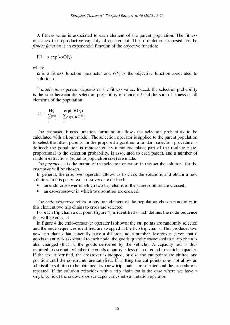
The endo-crossover refers to any one element of the population chosen randomly; in

this element two trip chains to cross are selected.

For each trip chain a cut point (figure 4) is identified which defines the node sequence

that will be crossed.

In figure 4 the endo-crossover operator is shown: the cut points are randomly selected

and the node sequences identified are swapped in the two trip chains. This produces two

new trip chains that generally have a different node number. Moreover, given that a

goods quantity is associated to each node, the goods quantity associated to a trip chain is

also changed (that is, the goods delivered by the vehicle). A capacity test is thus

required to ascertain whether the goods quantity is less than or equal to vehicle capacity.

If the test is verified, the crossover is stopped, or else the cut points are shifted one

position until the constraints are satisfied. If shifting the cut points does not allow an

admissible solution to be obtained, two new trip chains are selected and the procedure is

repeated. If the solution coincides with a trip chain (as is the case where we have a

single vehicle) the endo-crossover degenerates into a mutation operator.


17

Figure 4: Endo-crossover: selection and crossing.

Eso-crossover refers to two solutions (parents) selected randomly, that are crossed.

The first step of the procedure is the selection of two trip chains (figure 5). The nodes

(clients) in the trip chains will be swapped as for the endo-crossover, obtaining two new

trip chains with a new sequence of nodes. However, the solution is temporary: two tests

are necessary to verify the solution. The first is an admissibility test: in general, in the

temporary solution there are some nodes repeated that must be eliminated. A search

procedure allows repeated nodes to be identified and eliminated. The second test is the

capacity test previously described for the endo-crossover.

The procedure is applied a number of times determined by the crossover rate. The

output is child population; some of the children are selected (according to the mutation

rate) and the mutation operator is applied. The mutation used considers, in a trip chain,

the swapping of two nodes. An example of mutation is shown in figure 6.

The output of the mutation is the child set. In this set we select the solution which has

the maximum fitness (and hence minimum cost), the fitness value being compared with

that of the previous solution: if the comparison satisfies the test for the last k iteration,

the procedure ends, or else it is iterated. In this case, the actual child set is the parent set

for the next generation.


18

Figure 5: Eso-crossover: selection, crossing and elimination.

Figure 6: Mutation: selection and swapping.


19

5. Application

This section is divided into two parts: in the first, some test cases are proposed to

evaluate performance and compare the solution provided by the algorithms proposed in

the previous section; in the second we report a study in a real case.

5.1. Test cases

Test cases differ in the number of delivery points, which vary from 3 to 14. To create

a test case the procedure described in sections 2 and 3 is simplified: the delivery point

positions are random generated and hence also the link cost. This is sufficient for a test

problem, but in a real case (section 5.2) it is necessary to apply the procedure reported

in section 3 (steps 1, 2 and 3) because user behaviour has to be simulated. Under this

simplifying assumption, the path cost is given and it is possible to apply a procedure to

combine the generated paths and solve the vehicle routing problem.

The exact approach provides the solution to be compared with those provided by the

heuristic algorithms. The solution provided by the iterated nearest insertion algorithm in

18% of cases coincides with the exact; in the other cases (82%) the variation in the

solutions varies from 2.5% to 24%.

The genetic algorithm was implemented using the following best calibrated

parameters:

FF variance = 0.00025

%crossover = 0.8

%mutation = 0.2

population size = 30

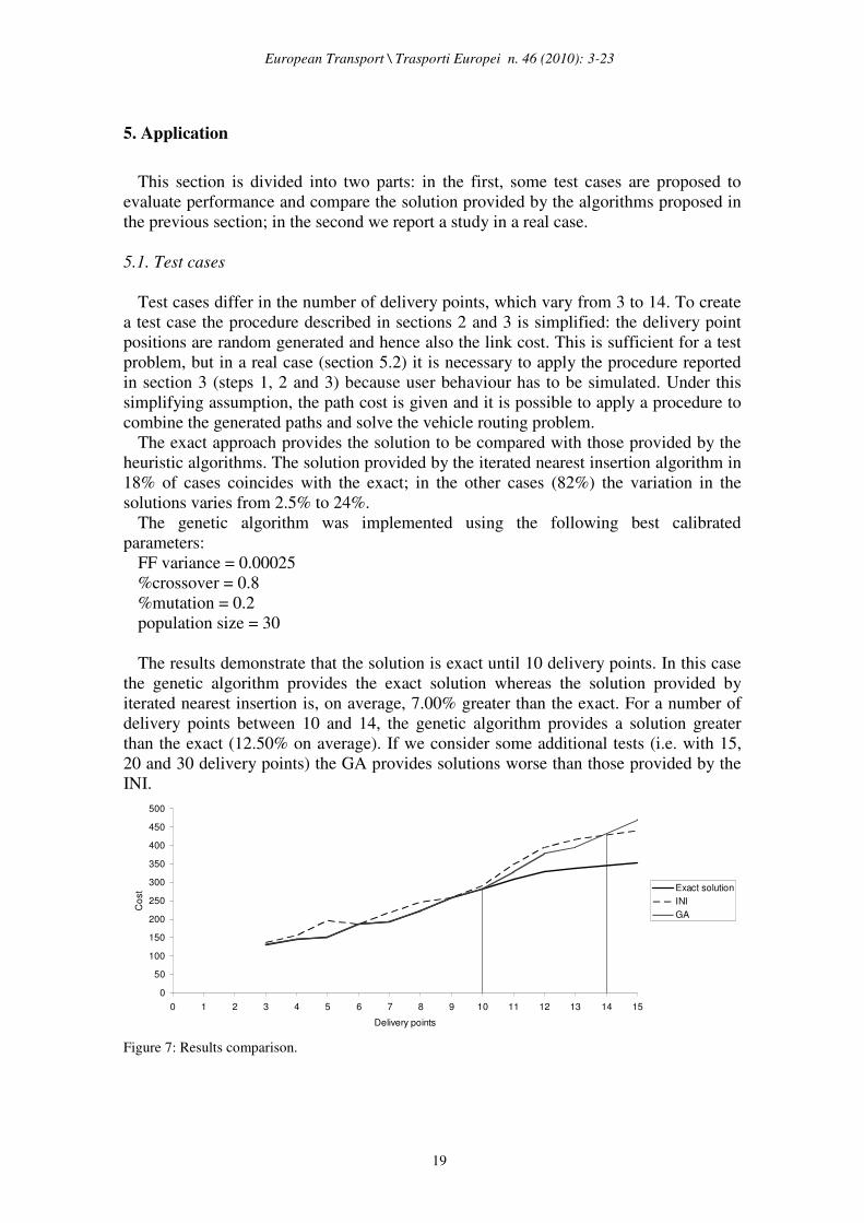
The results demonstrate that the solution is exact until 10 delivery points. In this case

the genetic algorithm provides the exact solution whereas the solution provided by

iterated nearest insertion is, on average, 7.00% greater than the exact. For a number of

delivery points between 10 and 14, the genetic algorithm provides a solution greater

than the exact (12.50% on average). If we consider some additional tests (i.e. with 15,

20 and 30 delivery points) the GA provides solutions worse than those provided by the

INI.

0

50

100

150

200

250

300

350

400

450

500

0 1 2 3 4 5 6 7 8 9 10 11 12 13 14 15

Delivery points

Co

st Exact solution

INI

GA

Figure 7: Results comparison.


20

Figure 7 reports the trend of the solutions found for each test. In addition, it also

highlights the points where:

• the GA deviates from the exact solution;

• the GA provides worse solutions than those provided by the INI.

An alternative procedure is the combination between the GA and INI to improve

solution goodness. In particular, the solution provided by the INI algorithm is inserted

in the population, replacing the worse element after a number of fixed iterations. The

tests demonstrate that, in some conditions, combined use of the genetic algorithm and

iterated nearest insertion gives a better solution than that found by using the algorithms

on their own (figure 8).

400

500

600

700

800

900

1000

1100

1200

1300

15 20 25 30 35 40 45 50

Delivery points

Cost INI

GA

GA & INI

Figure 8: Combination of algorithms.

5.2. Real case

The application focuses on a real case of goods distribution in an urban area. The

database concerns a sample of 1862 retailers and information collected during a survey

on supply and goods distribution in the city of Palermo (CSST, 1998). Analysis showed

that 17% of the retailers supply their shops on their own. Of these, 75% choose the

delivery points inside the city. Focusing attention on the latter, some retailers go to the

fish market and the fruit and vegetable market: these retailers have time windows to

respect (market opening/closing); others go to various delivery points (food, stationery

and so on). We assume that operation time is a function of the goods quantity delivered.

In relation to the framework proposed in the previous sections (figure 1) the

application refers to the vehicle level, in particular to the path choice (third zoom

aggregation) and to VRP (fourth zoom aggregation). Note that the VRP is addressed as

the search of a paths combination that minimizes the total cost. Moreover, the goods

quantity (first zoom aggregation) is that observed.

We consider two cases:

A) a retailer who supplies his shop using a single vehicle,

B) a carrier who supplies retailers using more than one vehicle.


21

In both cases, the approach adopted is that described in section 2. In the first step,

through traffic assignment, the travel time for each element of the network is

determined. In the second step, the one-to-one problem is solved by considering the

travel time found in the first step. In the case (A), known the retailer shop position and

the delivery points’ position, the shortest paths between all possible origin-destination

pairs (shop-delivery point, delivery point- delivery point, delivery point- shop) can be

determined. In the case (B) the carrier depot position and the shop positions are knew;

the procedure used is similar of case (A). In the third step the shortest paths are

combined to find the best routes. The shortest paths combination allows to determinate a

path sequence which: case A) start from the shop and go back in it, visiting the delivery

points in a certain order; case B) start from the carrier depot and go back in it, visiting

the shops in a certain order.

In the case (A) we have a retailer that visit four delivery points. The solution

procedure applied (exact algorithm, GA, INI algorithm and GA & INI combination)

give the same solution.

In case (B) we applied the GA, the INI algorithm and the GA & INI combination.

Two versions of the GA are also applied (see section 4.2): GA with single crossover

(GA1) and GA with double crossover (GA2). In this case, the carrier does the deliveries

using a fleet of four vehicles. The results are shown in figure 9.

0.00

1.00

2.00

3.00

4.00

5.00

6.00

7.00

8.00

9.00

10.00

Cost x 1

0^2 GA1

GA2

INI

GA1 & INI

GA2 & INI

Figure 9: Case B): results comparison.

6. Conclusion

In this paper, a method to study the retailer’s delivery approach is presented. A

macro-architecture is reported for a model system to simulate goods movements in an

urban area when the retailer is the decision-maker. In the macro-architecture four

subsequent zooms are distinguished in which goods movements are analysed from the

upper macro-levels (commodity and vehicle level) to path choice. Path choice is

analysed by considering two problems: the one-to-one problem and the vehicle routing


22

problem. The one-to-one problem is tackled in two cases: the mono-path case with a

deterministic approach and the multi-path case with a probabilistic approach. The

vehicle routing problem is formulated as a combinatorial problem whose objective is to

determine the best combination of one-to-one paths in order to visit a certain number of

nodes in succession: a multi-path vehicle routing problem is considered. Calculation of

the shortest path requires analysis of the transport system and definition of the flow and

cost vectors: to this end some methods (traffic assignment; real time cost measurement;

reverse assignment) are reported.

The vehicle routing formulation involved definition of some cost terms – travel time,

operation time and penalty time – to allow for various aspects of the problem – travel,

operations and delay/advance.

To solve the problem we propose an exact procedure (explicit enumeration of all

solutions), a greedy algorithm and a genetic algorithm; the results obtained have been

compared. It emerges that for a small number of delivery points (<10) the genetic

algorithm provides the exact solution whereas the solution provided by iterated nearest

insertion is, on average, 7.00% greater than the exact. For a number of delivery points

between 10 and 14, both the genetic algorithm and the iterated nearest insertion provide

a solution greater than the exact (12.50% and 15.50% respectively).

For a number of delivery points greater than 14, the genetic algorithm provides a

solution greater than that provided by iterated nearest insertion. This suggests that for a

high node number it is advisable to combine the two algorithms into a hybrid algorithm

to assist convergence. A first test from combining the genetic algorithm and iterated

nearest insertion is proposed. Future calibration of the demand model is scheduled and

application to a larger, real case will be studied. Implementation of a hybrid algorithm

(genetic and nearest insertion) is also scheduled.

References

Almeida, M.T., Schützc, G. and Carvalho, F.D. (2008) “Cell suppression problem: a genetic-based

approach”, Computers & Operations Research 35: 1613 - 23.

Ando, N. and Taniguchi, E. (2006), “Travel Time Reliability in Vehicle Routing and Scheduling with

Time Windows”, Networks and Spatial Economics 6: 293-311.

Antonisse, R.W., Daly, A.J. and Ben Akiva, M. (1985) “Highway assignment method based on

behavioural models of car driver’s route choice”, Transportation Research Record 1220: 1-11.

Baker, B.M. and Ayechew, M.A. (2003) “A genetic algorithm for the vehicle routing problem”,

Computers & Operations Research 30: 787 – 800.

Baldacci, R., Christofides , N. and Mingozzi, A. (2008) “An exact algorithm for the vehicle routing

problem based on the set partitioning formulation with additional cuts”, Mathematical Programming

15 (2): 351- 85.

Beckman, M., McGuire, C.B. and Winsten C.B. (1956) Studies in the economics of transportation, Yale

University Press, New Haven.

Ben Akiva, M., Bergman, M.J., Daly, A.J. and Ramaswamy, R. (1984) “Modelling interurban route

choice behaviour”, Proceedings from 9th International Symposium on Transportation and Traffic

Theory, VNU Science Press.

Ben-Akiva, M., Bierlaire, M., Koutsopoulos, H. and Mishalani, R. (1998) “DynaMIT: a simulation-based

system for traffic prediction and guidance generation”, Proceedings from TRISTAN III, San Juan.

Cascetta, E. (2009) Transportation Systems Analysis: Models and Applications, Springer.

Cascetta, E., Nuzzolo, A., Russo, F. and Vitetta, A. (1996) “A new route choice logit model overcoming

IIA problems: specification and some calibration results for interurban networks”, Proceedings from

the 13th International Symposium on Transportation Traffic Theory (Jean-Baptiste Lesort eds),

Pergamon Press.


23

CSST (1998) “Indagine conoscitiva sulla raccolta e distribuzione delle merci nella città di Palermo”,

Centro Studi sui Sistemi di Trasporto, S.p.A. Napoli.

Dantzig, G.B. and Ramser, J.H. (1959) “The Truck Dispatching Problem”, Management Science; 6 (1):

80-91.

Fisher, M.L. (1994) “Optimal solution of vehicle routing problems using minimum k-trees”, Operation

Research 42: 626-42.

Gendreau, M., Potvin, J.Y., Bräysy, O., Hasle, G. and Løkketamgen, A. (2008) “Metaheuristics for the

vehicle routing problem and its extensions: a categorized bibliography”, In: Golden, B., Raghavan, S.

and Wasil E. (eds) The vehicle routing problem: latest advances and new challenges, Springer, New

York.

Hanshar, F.T. and Ombuki-Berman, B.M. (2007) “Dynamic Vehicle Routing Using Genetic Algorithms”,

Appl. Intell. 27: 89-99.

Harker, P.T. (1985) Predicting intercity freight flows, VNU Science Press, Utrecht.

Hoose, N. (1991) Computer image processing in traffic engineering, John Wiley & Sons Inc.New York.

Hu, X., Huang, M. and Zeng, A.Z. “An Intelligent Solution System for a Vehicle Routing in Urban

Distribution”, International Journal of Innovative Computing, Information and Control 3 (1): 189 - 98.

Jones, D.F., Mirrazavi, S.K. and Tamiz, M. (2002) “Multi-objective meta-heuristics: an overview of the

current state of the art”, European Journal of Operational Research 137: 1-9.

Jozefowiez, N., Semet, F. and Talbi, E.G. (2009) “An evolutionary algorithm for the vehicle routing

problem with route balancing”, European Journal of Operational Research 195: 761–769.

Laporte, G. (2007) “What You Should Know about the Vehicle Routing Problem”, Les Cahiers du

GERAD, G-2004-33, HEC Montreal (www.gerad.ca/en/publications/cahiers.php).

Laporte, G., Gendreau, M., Potvin, J.Y. and Semet, F. (2000) “ Classical and modern heuristics for the

vehicle routing problem”, International Transaction in Operational Research 7: 285-300.

Malandraki, C., Daskin, M.S. (1992) “Time dependent vehicle routing problems: formulation, properties

and heuristic algorithms”, Transportation Science 26: 185–200.

Manski, C. (1977) “The structure of random utility models”, Theory and Decision 8; 229-254.

Montemanni, R., Gambardella, L.M., Rizzoli, A.E. and Donati, A.V. (2005) “ Ant Colony System for a

Dynamic Vehicle Routing Problem”, Journal of Combinatorial Optimization 10: 327- 343.

Ogden, K.W.(1992) Urban Goods Movement: a Guide to Policy and Planning, Ashgate Publishing

Limited, Aldershot (UK).

Russo, F. and Vitetta, A. (2003) “An assignment model with modified Logit, which obviates enumeration

and overlapping problems”, Transportation 30: 177-201.

Russo, F. and Vitetta, A. (2005) “Reverse assignment: Updating demand and calibrating cost jointly from

traffic counts and time measurements”, Proceedings from International Symposium on Transportation

and Traffic Theory, Maryland University.

Russo, F. and Vitetta, A. (2006) La ricerca di percorsi in una rete: Algoritmi di minimo costo ed

estensioni, FrancoAngeli, Milan.

Russo, F., Comi, A. (2006) “ Demand models for city logistics: a state of the art and a proposed

integrated system”, Proceedings from 4th International Conference on City Logistics (Thompson, R.G.,

Taniguchi, E. eds.), Elsevier Ltd., United Kingdom.

Russo, F., Comi, A. (2010) “A modelling system to simulate goods movements at an urban scale”,

Transportation, 37(6): 987-1009.

Russo, F., Polimeni, A. and Comi, A. (2007) “Urban freight transport and logistics: retailer’s choices”, In:

Taniguchi E., Thompson R.G. (eds) Innovations in City Logistics, Nova Publisher, New York.

Sheffi, Y. (1985) Urban transportation network, Prentice-Hall Inc, Englewood Cliffs.

Taniguchi, E., Ando, N. and Okamoto M. (2007) “Dynamic vehicle routing and scheduling with real time

travel times on road network”, Journal of the Eastern Asia Society for Transportation Studies 7:

1138 – 53.

Torday, A. and Dumont, A.G. (2004) “Probe vehicles based travel time estimation in urban networks”,

Proceedings of TRISTAN V, Guadaloupe.

Toth P. and Vigo, D. (2002) “Models, relaxations and exact approaches for the capacitated vehicle

routing problem”, Discrete Applied Mathematics 123: 487-512.

Wang, C.H. and Lu, J.Z. (2009) “A hybrid genetic algorithm that optimizes capacitated vehicle routing

problems”, Expert Systems with Applications 362: 2921- 2936.

Wardrop, J. P. (1952) “Some theoretical aspects of road traffic research”, Proceedings from the Institute

of Civil Engineers, Part II (1).

Documents

Demand and routing models for urban goods movement …