Embed Size (px)
DESCRIPTION
Delivery Time Timing Using Packet Networks Tommy Cook Calnex
Citation preview

Delivery of Time & Timing using Packet Networks Tommy Cook, CEO

Proving performance of;
• EEC - Synchronous Ethernet Devices.
• 1588v2 Devices.
• Boundary Clocks.
• Transparent Clocks.
• Ordinary Clocks.
• Networks
• Packet Network Metrics
• Networks with slave devices (experimental results)
Presentation overview
2

EEC – Synchronous Ethernet devices

04
100M/1G/10G SyncE
Synchronisation Source
EEC
Ref
100M/1G/10G SyncE
Wander generation
Wander tolerance
Wander transfer
Frequency Accuracy
Pull-in, Pull-out, Hold-in
SyncE Under Test
SyncE (Wander-free)
EEC
Ref
Phase transient response
Sync-E Wander to G.8262

Measure Jitter
SyncE (Jitter-free)
EEC
Ref
1) Jitter generation 2) Jitter tolerance
SyncE + Jitter
Measure Dropped Packets. Monitor ESMC Status.
• No dropped packets indicating bit errors being introduced.
• Not causing any alarms.
• Not causing the clock to switch reference.
Ref
EEC
Sync-E Jitter to ITU-T G.8262

1588v2 Devices
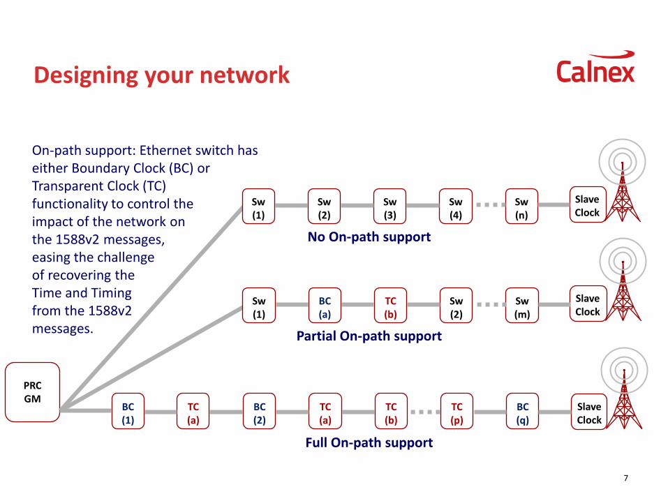
Designing your network
7
Slave Clock
Slave Clock
On-path support: Ethernet switch has either Boundary Clock (BC) or Transparent Clock (TC) functionality to control the impact of the network on the 1588v2 messages, easing the challenge of recovering the Time and Timing from the 1588v2 messages.
Sw (m)
Sw (2)
TC (b)
BC (a)
Sw (1)
BC (q)
TC (p)
TC (b)
TC (a)
BC (2)
TC (a)
BC (1)
PRC GM
Slave Clock
Sw (n)
Sw (4)
Sw (3)
Sw (2)
Sw (1)
No On-path support
Partial On-path support
Full On-path support

Boundary Clocks

Boundary Clock
9
Boundary Clocks reduce PDV accumulation by;
• Terminates the PTP flow and recovers the reference timing.
• Generate a new PTP flow using the local time reference, (which is locked to the recovered time).
• No direct transfer of PDV from input to output.
Boundary Clock is in effect a back-to-back Slave+Master.
Q2
Qn
Q1
Clock
Slave Master

Performance specification of a T-BC
Draft ITU-T G.8273.2 will specify the performance of a BC. A number of sections have been proposed;
6. Physical Layer Performance requirements (G.8262 when SyncE supported)
7. Packet layer performance requirements
7.1 Noise Generation
7.1.1 Constant time error generation
7.1.2 Time noise generation
7.2 Time Noise Tolerance
7.3 Time Noise Transfer
7.4 Packet Layer Transient and Holdover Response
The structure in G.8273.2 is following the well established methods of specifying the performance of node clocks (e.g. in G.8262 for SyncE, etc.) but with the additions particular to the transfer of Time.

Master Slave
Impairment
1pps Meas
Freq.Meas
Capture Capture
Ref. Time & Freq.
Clock
Slave Master
T-BC Time Error (TE) TE: Difference between recovered
time in the T-BC to the Master’s Time.
• Max TE (absolute wrt ref)
• Dynamic TE, MTIE/TDEV • Constant TE (absolute wrt ref)
a) Measure 1pps;
• If 1pps available, compare to 1pps from Master reference to determine accuracy.
b) Measure Egress 1588v2;
• Analysis timestamps to determine TE of T-BC.
• Need to include t1 and t4 delays to measure Time output as seen by downstream device.
Freq.
Ingr
ess
15
88
v2
Reference Plane
1pps
Measurement point
t1 delay
t4 delay
Egress 15
88
v2

T-BC test results example
Stimulus; • TDEV SyncE noise
injected to ingress port.
Measurement; • Frequency Response • Time Response
Freq. Response, 2M Clock output
Time Response, 1pps output
810nsec pk-to-pk Max. TE = 155nsec Constant TE = 14nsec
Clock Slave Master
Freq. 1pps
Devices that utilise SyncE, it is important to verify; • SyncE performance to G.8262. • Time transfer performance to G.8273.2, (under dev.).
• As well as tolerance to 1588v2 noise, check Time performance when exposed to SyncE physical layer noise.

Transparent Clocks
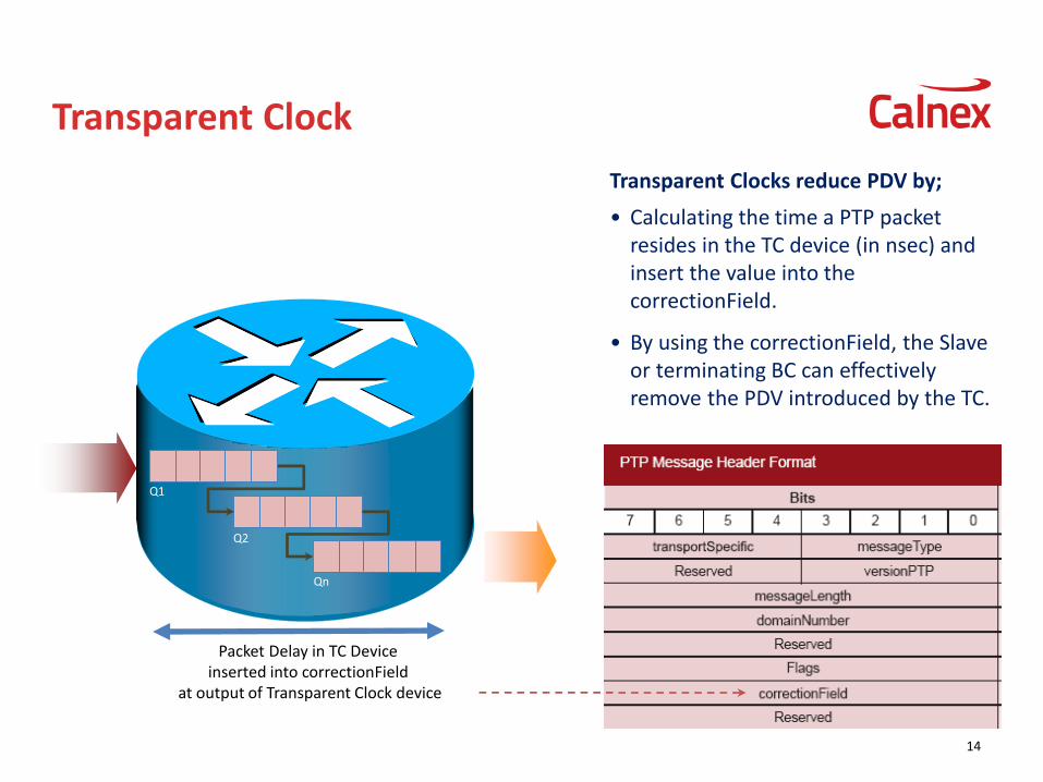
Transparent Clock
14
Q1
Q2
Qn
Packet Delay in TC Device inserted into correctionField
at output of Transparent Clock device
Transparent Clocks reduce PDV by;
• Calculating the time a PTP packet resides in the TC device (in nsec) and insert the value into the correctionField.
• By using the correctionField, the Slave or terminating BC can effectively remove the PDV introduced by the TC.

Accuracy of the CorrectionField value:
15
Q1
Q2
Qn
Types of CorrectionField inaccuracy;
1. Variable error • Caused by packet-to-packet variation in
CorrectionField accuracy. • Leads to residual PDV when PTP terminated.
2. Fixed Error
• Caused by CorrectionField value always being greater than a fixed value.
• Results in a fixed delay being measured when PTP terminated.
• Not as issue if Fixed Error is matched in forward and reverse direction.
• Differences between forward and reverse Fixed Error will produce asymmetry and hence create a fixed Time Error.
Theoretical model:
•CorrectionField precisely reflects the delay through the equipment
• Ideal case – zero net PDV
Does it reflect the actual delay experienced by the Sync & Del_Req messages?

Transparent Clock Test Plan
16
Development Test Procedure to characterise actual performance
1. Measure the packet-by-packet latency across the TC.
2. Determine the change to the correctionField value for each message.
3. Accuracy is the difference in the actual latency compared to the change in Correctionfield value.
• Measure impact of CorrectionField on Sync PDV.
1. Vary traffic packet size.
2. Vary traffic priority.
3. Vary traffic utilisation.
• Repeat for Sync & Del_req PDV. Test in 1-Step and 2-Step modes.
IEEE std C37.238-2011 PTP in Power Systems Applications.
• Annex A: TC TimeInaccuracy ≤50nsec.
TC
Traffic from Traffic Generator for Congestion noise testing
Optical Splitter or Electrical Tap
•`1` Master
Clock •`1` Slave
Clock

TC CorrectionField Accuracy example results
0.36
0.35
0.34
0.33
0.32
Variable Error = 35nsec Fixed Error = 320nsec

Ordinary Clocks
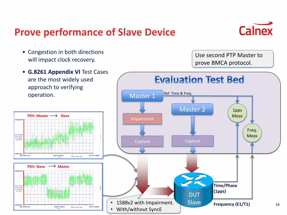
Prove performance of Slave Device
19
895.477518885 894.977768110 894.478017335 Offset=0.002 ppm
-0.00029635
0.00064588
Time Interval Error (TIE) vs Nominal (seconds)
T (a)
895.477518885 894.977768110 894.478017335 Offset=0.002 ppm
-0.00029635
0.00064588
Time Interval Error (TIE) vs Nominal (seconds)
T (a)
PDV: Master Slave
PDV: Slave Master
• Congestion in both directions will impact clock recovery.
• G.8261 Appendix VI Test Cases are the most widely used approach to verifying operation.
Time/Phase (1pps)
Frequency (E1/T1)
Test Bed
• 1588v2 with Impairment. • With/without SyncE
Use second PTP Master to prove BMCA protocol.
DUT Slave
Master 1
Master 2 Impairment
1pps Meas
Freq.Meas
Capture Capture
Ref. Time & Freq.

Networks
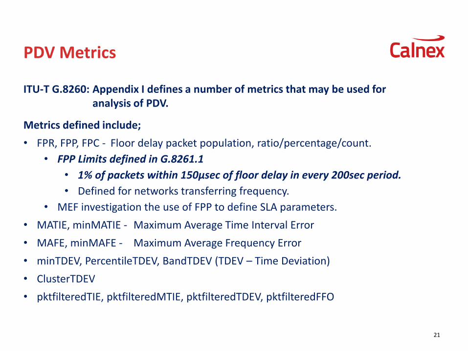
ITU-T G.8260: Appendix I defines a number of metrics that may be used for analysis of PDV.
Metrics defined include;
• FPR, FPP, FPC - Floor delay packet population, ratio/percentage/count.
• FPP Limits defined in G.8261.1
• 1% of packets within 150µsec of floor delay in every 200sec period.
• Defined for networks transferring frequency.
• MEF investigation the use of FPP to define SLA parameters.
• MATIE, minMATIE - Maximum Average Time Interval Error
• MAFE, minMAFE - Maximum Average Frequency Error
• minTDEV, PercentileTDEV, BandTDEV (TDEV – Time Deviation)
• ClusterTDEV
• pktfilteredTIE, pktfilteredMTIE, pktfilteredTDEV, pktfilteredFFO
PDV Metrics
21

Packet Metrics, example result
22
Frequency
Time/Phase
MAFE
Mask: NSN HRM-2
Parameters:
• Floor Packets
• 10 minimum in 100sec window.
• 1500sec averaging filter
• Scaling 0.65
pktfilteredMTIE/TDEV on Sync: PDF – Probability Density Function
• 70 of packets within 150µsec cluster
band from floor delay within every
200sec window.
FPC – Floor Packet Count
G.8261.1 Network Limit;
• 1% of packets within 150µsec cluster
band from floor delay within every
200sec window.
FPP – Floor Packet Percentage
DUT Slave E1 MTIE/TDEV
1pps TIE

Network with Slave (example)

Test network
24
Sw#1
Sw #2
Sw #3
Sw #9
Slave Master
Traffic Generator
Ethernet Connection
Congestion traffic
1pps
~
Network PDV Monitor
Wander Monitor
E1
Traffic from G.8261 Appendix VI: • Test Case 13 • Traffic Model 2
Experimental Network Configurations; 1. 9 switches, No On-path Support, No SyncE PTP for Frequency & PTP for Phase 2. 9 switches, all BC mode, SyncE SyncE for Frequency & PTP for Phase 3. 9 switches, all BC mode, No SyncE PTP for Frequency & PTP for Phase 4. 9 switches, all TC mode, SyncE SyncE for Frequency & PTP for Phase 5. 9 switches, all TC mode, No SyncE PTP for Frequency & PTP for Phase

Results: BC networks
25
BC #1
BC #2
BC #3
BC #9
Slave Master
Traffic Generator
Ethernet Connection
Congestion traffic
1pps
~
Network PDV Monitor
Wander Monitor
E1
Test Set-up PDV at input to
slave
E1 wander (MTIE @ 5000sec)
1pps (pk-to-pk)
9xSw w/o SyncE 86µsec 2.44µsec 2.70µsec
9xBC w/o SyncE 0.105µsec 0.210µsec 0.220µsec
9xBC with SyncE 0.055µsec 0.019µsec 0.028µsec
Observations when BCs utilised; • SyncE (EEC) + PTP gave the best results. • BCs reduce the impact of congestion traffic,
but congestion can still impact the transfer of frequency &/or Phase.
Sync PDV: 105nsec pk-pk
Sw Sw Sw Sw

Results: TC networks
26
TC #1
TC #2
TC #3
TC #9
Slave Master
Traffic Generator
Ethernet Connection
Congestion traffic
1pps
~
Network PDV Monitor
Wander Monitor
E1
Test Set-up PDV at input to
slave
E1 wander (MTIE @ 5000sec)
1pps (pk-to-pk)
9*Sw w/o SyncE 86µsec 2.44µsec 2.70µsec
9*TC w/o SyncE 245nsec (86µsec)*
1.10µsec 1.75µsec
9*TC with SyncE 0.137µsec 0.112µsec
Observations when TCs utilised; • SyncE (EEC) + PTP gave the best results. • TCs reduce the impact of congestion traffic,
but congestion can still impact the transfer of frequency &/or Phase.
PDV: 86µsec pk-pk, without CF
PDV: 0.245µsec pk-pk, with CF

• SyncE
• 1588v2
• BC
• TC
• Ordinary Clocks
• Networks
Summary of Evaluation Plan
27
•Characterise using G.8261 Appendix VI test cases. •Measure
• Frequency Accuracy. • Time Accuracy.
•Prove accuracy of CorrectionField. • Fixed Error, Variable Error, Asymmetry.
•IEEE Std C37.238-2011 ‘PTP in Power Systems Applications’ • Profile specify ≤50nsec.
•G.8273.2 Standard under development. • Time Noise Generation • Time Noise Tolerance • Time Noise Transfer • Phase Transient & Holdover;
•Consider behaviour during Traffic Congestion.
•Standards in force. •G.8262
• Wander • Jitter
•G.8264 • ESMC behaviour
•Metrics specified in G.8260 Appendix I. • FPP, limit in G.8261.1 • MAFE, minTDEV, etc • pktfilteredMTIE, pktfilteredTDEV
•Evaluate selected devices with Network.