Deliverable Documentation Scenario Tree Tool - wilmar.risoe.dk d6_2_d_ScenarioTree_doc.pdf · Documentation Scenario Tree Tool 5 1 Preface This report is a documentation of the used

University of Stuttgart Institute of Energy Economics and the Rational Use of Energy

WILMAR Deliverable 6.2 (d)

Documentation

Methodology of the

Scenario Tree Tool Rüdiger Barth, Lennart Söder, Christoph Weber, Heike Brand, Derk Jan Swider

January 2006

.

.

.

.

.

.

.

.

.

.

.

.

Institute of Energy Economics and the Rational Use of Energy (IER) University of Stuttgart Hessbruehlstrasse 49a

70565 Stuttgart, Germany c/o Dipl.-Ing. Rüdiger Barth

Tel: ++49-711-780-6139 Fax: ++49-711-780-3953

e-Mail: [email protected] Internet: http://www.ier.uni-stuttgart.de

Documentation Scenario Tree Tool

3

Contents

1 PREFACE.......................................................................................................................5

2 METHODOLOGIES OF THE MODULES OF THE SCENARIO TREE TOOL .7

2.1 Wind Speed Forecast Error Module ........................................................................7 2.1.1 Methodology for one single measurement station ...................................................7 2.1.2 Correlation of wind speed forecast errors ................................................................9

2.2 Wind2PowerAggregate Module..............................................................................11

2.3 Scenario Reduction Module ....................................................................................13 2.3.1 Scenario reduction..................................................................................................14 2.3.2 Creation of a multi-stage scenario tree ..................................................................15 2.3.3 Example..................................................................................................................18

2.4 Wind Power Forecast Errors For SPF Module.....................................................24

3 REFERENCES.............................................................................................................27


5

1 Preface

This report is a documentation of the used methodologies of the individual modules of the Scenario Tree Tool. It is part of the project Wind Power Integration in Liberalised Electricity Markets (WILMAR) supported by EU (Contract No. ENK5-CT-2002-00663). The task of the Scenario Tree Tool is to generate scenarios trees of wind power forecasts for the Joint Market Model (compare deliverable 6.2 (b) of the WILMAR project) and of wind power forecast errors for the Stepwise Powerflow Model (compare deliverable 5.1 of the WILMAR project) on the basis of given wind speed and wind power data. Thereby scenarios of wind speed forecasts are simulated for each individual time step by applying a Monte-Carlo-simulation on an econometric approach with the “Wind speed forecast module”. The generated wind speed forecast scenarios are transformed into wind power forecast scenarios by the “Aggregated power curve module” and reduced to a scenario tree by the “Scenario reduction module”. Wind power forecast errors are determined with the module “Wind Power Forecast Errors for SPF.”


6


7

2 Methodologies of the modules of the Scenario Tree Tool

In the following a description of the methodologies used by the individual modules of the Scenario Tree Tool is given.

2.1 Wind Speed Forecast Error Module

The Wind Speed Forecast Error Module simulates for each hour a set of realistic wind speed prediction scenarios on hourly basis and up to 36 hours days ahead. The development of this module is based on /Söder 2004/. The simulated wind speed prediction scenarios include: • The autocorrelation of the wind speed forecast errors over the forecast length for a

specific wind speed measurement station. • The correlations of the wind speed forecast errors between individual wind speed

measurement stations for the individual forecast hours. Within the approach it is assumed that data concerning the accuracy of wind speed forecasts in different regions and the correlations of the wind speed prediction errors are known.

2.1.1 Methodology for one single measurement station

The used simulation method has to generate realistic possible outcomes of wind speed forecast errors with correct statistical behavior and correlation between different measurement stations. The method uses an ARMA(1,1) approach, i.e. Auto Regressive Moving Average series. This series is defined as

(2-1)

where X(k) = wind speed forecast error in forecast hour k ∈ N Z(k) = random Gaussian variable with standard deviation σZ in forecast hour k ∈ N α, β = parameter of the ARMA-series. With this approach the wind speed forecast errors are simulated (compare Figure 2-1). The assumed wind speed forecasts for each hour can then be calculated as the sum of the measured wind speed time-series and the wind speed forecast error.

)1()()1()(0)0(0)0(

−++−===

kZkZkXkXZX

βα


8

0 5 10 15 20 25 30-4

-3

-2

-1

0

1

2

3

4

Fore

cast

err

or [m

/s]

Forecast length [h]

Figure 2-1: Four examples of ARMA(1,1)-outcomes of wind speed forecast errors with assumed ARMA-parameters α=0.95, β=0.02 and σZ=0.5.

The variance of the ARMA(1,1) model, i.e. the variance of X(k), can be calculated in the following way:

(2-2)

For 2≥k , this equation can be rewritten as

(2-3)

The standard deviation of the forecast error is then calculated as (2-4)

In Figure 2-2, the standard deviation for the ARMA(1,1) series with the ARMA-parameters assumed in Figure 2-1 are shown together with the standard deviation of 50 different outcomes. The identification of the ARMA-parameters α, β and σZ is not processed within the Scenario Tree Tool. The parameters are derived from data describing wind speed forecast errors for Eastern Denmark in 2003. Therefore an extended method of /Söder 2004/ has been used.

222

2

)21()1()()1(

0)0(

Z

Z

kVkVVV

σαββασ

+++−=

=

=

⎟⎠

⎞⎜⎝

⎛+++= ∑

=

−−k

i

ikZkV

1

)1(2)1(22 )21()( ααββασ

( ) )()( kVkX =σ


9

0 5 10 15 20 25 300

0.5

1

1.5

2

0 5 10 15 20 25 300

0.2

0.4

0.6

0.8

1 Maglarp-Bösarp "+", Maglarp-Sturup "o", Näsudden-Ringhals "*"

time t

rho(

t)

Figure 2-2: Forecast error standard deviation over the forecast hour: analytical (straight line), 50 series (dashed line).

2.1.2 Correlation of wind speed forecast errors

When wind speeds are forecasted for the same time period but for different locations, the forecast errors will be correlated because unpredicted wind conditions will affect both sites. The short time forecast errors of two measurement stations that are far from each other are assumed to be less correlated, since the unpredictable wind situations are not the same for the two sites. For longer forecasts the unpredictable wind conditions are though similar for the two stations, so the forecast errors become more correlated. In Figure 2-3 three examples of correlations between wind speed forecast errors are shown. As no real wind speed forecasts have been available for these measurement stations, it has been assumed that persistence forecasts have been used.

Figure 2-3: Correlation between forecast errors for different pairs of stations. The distances

between the stations are Maglarp-Bösarp (15 km), Maglarp-Sturup (26 km), Näsudden-Ringhals (370 km).

In the Figure 2-3 it is obvious that the closer the stations are, the higher the correlation between forecast errors becomes. Thereby the correlation increases with the forecast length. The correlation compared to Figure 2-3 will probably decrease with better forecast methods because the forecast errors will then probably depend more on local (uncorrelated) unpredictable changes.


10

The used method simulates the correlations with a multidimensional ARMA-model. Since the correlation increases with time, the added uncertainty at different sites has to be more similar when the forecast horizon increases. Therefore the Z-variables in the ARMA- series should have an increased correlation if the correlations between the resulting X-variables increase. The method adds a correlated Gaussian matrix CZZ to the individual ARMA-series Xk considering the assumption that the standard deviation of the common Gaussian variable Z(k) is constant. The derivation of the correlated Gaussian matrix CZZ works as follows. The covariance between for example two wind speed measurement stations is calculated with:

)()(*)()( 211212 kVkVkkC XX ⋅= ρ (2-5)

where C12(k) = covariance for the forecast hour k ∈ N ρ12(k) = given correlation between the individual measurement stations for the forecast hour k ∈ N Vx(k) = variance for the forecast hour k ∈ N The correlated Gaussian matrix CZZ can now be calculated with:

)ˆˆ)(1()ˆˆ(ˆ))1()1((ˆ)()(

)1()1(0)0(

1212

12

βαβααα +−+−−−−−=

==

kCkCkCkCkC

CCC

ZZZZZZ

ZZ

ZZ

(2-6)

where CZZ = correlated Gaussian matrix C12(k) = covariance for the forecast hour k ∈ N

βα ˆ,ˆ = diagonal matrix containing the elements of α and β

The correlation between the individual ARMA-series X(k) is constant, equal to the correlation between the Gaussian variables Z and independent of the regarded hour. The standard deviations of the Gaussian variables do not have to be the same, thus the variances of the individual ARMA-series X(k) do not have to be the same. For the generation of the wind speed forecast error scenarios, the eigenvalues (D) and eigenvectors (V) of the correlated Gaussian matrix CZZ are determined. In the style of the Cholesky decomposition the matrix M is derived with:

DVM= (2-7)


11

To generate the scenarios for each individual forecast hour there is the option to draw firstly one scenario of the Gaussian variable by multiplying the matrix M with a normally distributed random value. This scenario is then treated as a simulation of the expected forecast error. Secondly a defined number of scenarios are generated by multiplying the M-matrix with the defined number of drawings of the normally distributed random values. This Monte-Carlo-simulation represents the uncertainty in the forecast. In the case that the single drawing has been made, it is finally added to these drawings.

2.2 Wind2PowerAggregate Module

The module “Wind2PowerAggregate” converts wind speed time-series and scenarios of wind speed forecasts into wind power time-series and scenarios of wind power forecasts by using an aggregated wind power curve. The following description of the methodology is based on /Norgard et al. 2004/ and /Norgard; Holtinnen 2004/. The power output from a single wind power turbine is depending on the short-term variation of wind speed at the location of the wind power turbine. Due to the spatial distribution of the individual wind turbines within a region in combination with the stochastic behaviour of wind speeds, the power outputs from different wind power turbines vary at the same time. Thereby the simultaneous power outputs from the individual wind turbines are assumed to be distributed around an average value and the deviation of the spatial distribution depends on the extent of the considered region. Thus the aggregated power generation from more wind power units in a certain area will smooth out the short-term fluctuations of wind speed, as the power generation from the individual units are not fully correlated. Typically the information of the instantaneous wind resource for an area is available in terms of only one time-series of the wind speed, valid only for the specific site, but representative for the entire area. The module “Wind2PowerAggregate Module” derives a time-series of the aggregated power generation from a cluster of wind turbines in a region on the basis of the time-series of the wind speed in a single point or alternatively on the basis of the time-series of power generation from a single wind power turbine or a smaller wind farm. Thereby it considers a standard wind power curve representative for all wind turbine units in question (it is assumed that all wind power turbines within the regarded area are similar in size and control principle) and the smoothing effects both in time and space. The methodology of the module “Wind2PowerAggregate Module” is described in the following step by step: 1. Specification of a representative dimension of the regarded region describing the

extent of the region in the NS and WE direction. This parameter is called “AreaSize”. 2. Specification of the wind speed distribution representative for the regarded regions by

defining the two Weibull distribution parameters (scale factor A and form factor k).


12

0%

10%

20%

30%

-6 -4 -2 0 2 4 6

Wind speed offset (m/s)

Prob

abili

ty (%

)

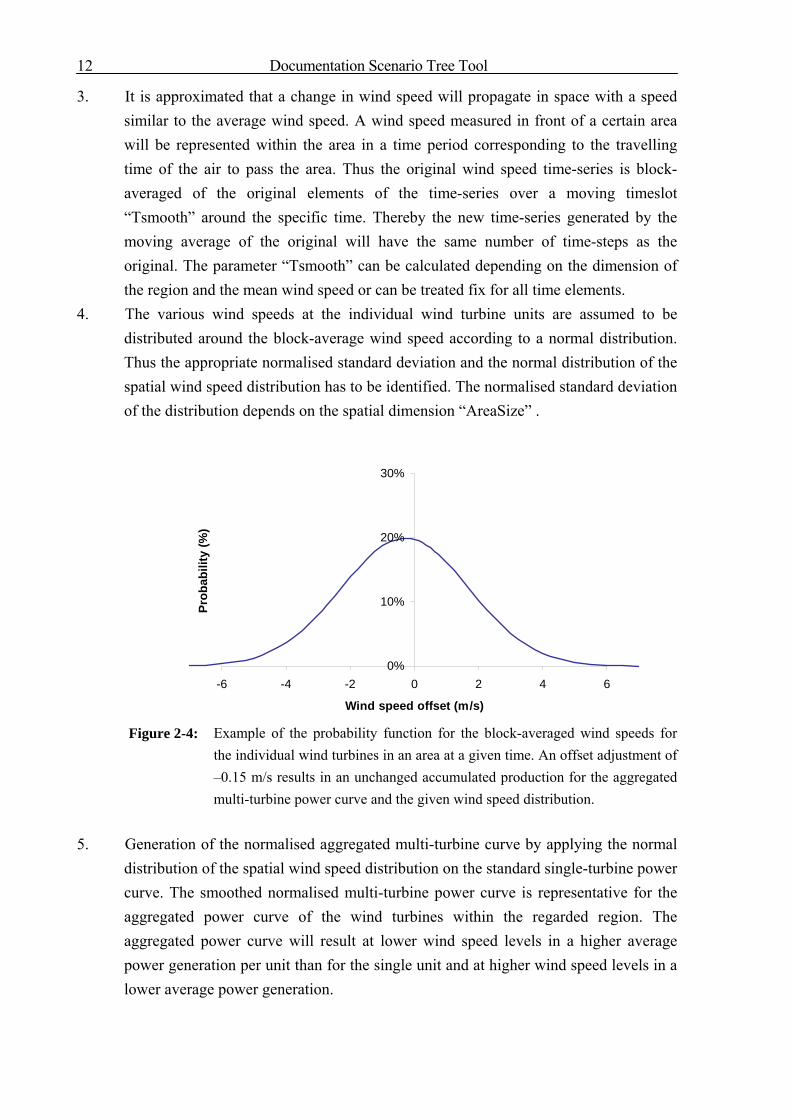
3. It is approximated that a change in wind speed will propagate in space with a speed similar to the average wind speed. A wind speed measured in front of a certain area will be represented within the area in a time period corresponding to the travelling time of the air to pass the area. Thus the original wind speed time-series is block-averaged of the original elements of the time-series over a moving timeslot “Tsmooth” around the specific time. Thereby the new time-series generated by the moving average of the original will have the same number of time-steps as the original. The parameter “Tsmooth” can be calculated depending on the dimension of the region and the mean wind speed or can be treated fix for all time elements.

4. The various wind speeds at the individual wind turbine units are assumed to be distributed around the block-average wind speed according to a normal distribution. Thus the appropriate normalised standard deviation and the normal distribution of the spatial wind speed distribution has to be identified. The normalised standard deviation of the distribution depends on the spatial dimension “AreaSize” .

Figure 2-4: Example of the probability function for the block-averaged wind speeds for the individual wind turbines in an area at a given time. An offset adjustment of –0.15 m/s results in an unchanged accumulated production for the aggregated multi-turbine power curve and the given wind speed distribution.

5. Generation of the normalised aggregated multi-turbine curve by applying the normal

distribution of the spatial wind speed distribution on the standard single-turbine power curve. The smoothed normalised multi-turbine power curve is representative for the aggregated power curve of the wind turbines within the regarded region. The aggregated power curve will result at lower wind speed levels in a higher average power generation per unit than for the single unit and at higher wind speed levels in a lower average power generation.


13

0.0

0.1

0.2

0.3

0.4

0.5

0.6

0 5 10 15 20 25 30

Wind speed (m/s)

Pow

er (p

er u

nit)

(kW

/m2)

Single Multiple

Figure 2-5: Example for normalised wind power curves corresponding to single and aggregated multi turbines.

6. The estimated normalised annual energy productions for a given wind speed

distribution in time (Weibull distribution) should be equal for the single- and multi-turbine power curve. This is obtained by comparing the normalised annual energy production and adjusting the offset of the spatial wind speed distribution found in step 4 until the energy productions of both power curves are equal.

7. Generation of the aggregated power curve for the considered region by upscaling the normalised aggregated power curve appropriately to the corresponding installed wind power capacity.

8. Generation of wind power time-series for the considered region by applying the aggregated wind power curve to the block-averaged wind speed time-series.

2.3 Scenario Reduction Module

The module “Wind Speed Forecast Error” (compare chapter 2.1) generates a large number of wind speed forecast error scenarios that are transformed into wind power scenarios by the “Wind to Power Aggregate Module” (compare chapter 2.2). For such huge numbers of scenarios it is impossible to numerically obtain a solution for the multi-stage optimisation problem. Moreover, the scenario tree consisting of these scenarios is only a one-stage tree. Thus, strategies for reducing the number of scenarios have to be studied to find a numerical solution of the problem as well as algorithms for constructing a multi-stage scenario tree out of a given set of scenarios. Simply generating a very small number of scenarios by Monte Carlo simulations is not wanted since less scenarios give less information. Indeed, the aim is to loose only a minimum of information by the reduction process applied to the whole set of scenarios. Actually, two steps are necessary: first, the pure number of scenarios is reduced. Afterwards, based on the remaining scenarios that still form a one-stage tree, a multi-stage scenario tree is constructed by deleting inner nodes and creating branching within the


14

0

1

2

3

4 5 6 7 8 9 10 11 12

stage 1 stage 2 stage 3

scenario tree. The chosen setup of the scenario tree used in the Joint Market Model is shown in Figure 2-6. It consists of a three stage tree with 9 leaves.

Figure 2-6: Setup of the scenario tree used in the Joint Market Model The following description of the scenario reduction and creation of the multi-stage scenario trees is partly based on /Brand et al. 2002/.

2.3.1 Scenario reduction

In the mathematical literature some algorithms are proposed for reducing a given set of scenarios and constructing a scenario tree based on the idea that the reduced scenario tree in a given sense is still a sufficient approximation of the original one /Dupacova et. al. 2000/. The Kantorovich distance ( )QPDKA , of a probability distribution P of a given number of

scenarios and a distribution of scenarios Q with given probabilities for each scenario has to be considered /Rachev 1991/. In the special case, that for Q a subset of all scenarios is chosen together with their probabilities, i.e. Q is a reduced probability distribution for P, an optimal probability distribution Q* based on these scenarios can be constructed possessing a minimal Kantorovich distance to P. A heuristic approach is used for finding the scenarios to be deleted from all scenarios /Dupacova et. al. 2000/. In the following the reduction algorithm is described in detail. Let Tn denote the

number of stages of the optimisation problem and Sn the number of scenarios. It is assumed

that all scenarios have a common root in a one-stage tree where branching occurs only after

the root node. A scenario )(iξ , { }Sni ,,2,1 K∈ , is defined as a sequence of nodes of the tree:

( ) Si

nii ni

T,,2,1,,, )()(

10)( KK == ηηηξ (2-8)

Where Si ni ,,2,1)(

00 K=∀= ηη denotes the root of all scenarios and )(inT

η denotes the leaf of

this scenario i within the tree. A node )( jsη belongs to scenario { }Snj ,,2,1 K∈ on stage

{ }Tns ,,2,1 K∈ . For each node )( jsη a vector

psnj

s R∈)(p of parameters is given. Each node )( j

sη has psn parameters. The probability to get from stage j to stage j+1 within scenario i, i.e.


15

to get from )(ijη to )(

1i

j+η , is denoted by )(1,

ijj +π . Thus the probability for the whole scenario )(iξ

is given by

∏−

=+=

1

0

)(1,

)(Tn

j

ijj

i ππ (2-9)

The distance between two scenarios )(iξ and )( jξ is defined as

( ) ( )2/1

0

2)()()()( , ⎟⎟⎠

⎞⎜⎜⎝

⎛−= ∑

=

Tn

s

js

is

jid ppξξ (2-10)

according to a norm in the space of the parameter vectors. So in a first step, the algorithm for deleting “whole” scenarios is described in the following. This deleting procedure is applied iteratively, deleting one scenario in each step and consequently changing the probabilities of other scenarios, until a given number of scenarios is remaining.

1. Determine the scenario to be deleted: Remove scenario ( )*sξ { }Sns ,,1* K∈ satisfying

( ) ( ){ }

( ) ( ))()(

,,1

)()( ,minmin,min*

*

* mn

mn

m

nm

ss

ss

s ddS

ξξπξξπ≠∈≠

=K

(2-11)

Intuitively it is clear that one tries to delete scenarios that are, according to the defined distance, near to some other scenario; otherwise possibly important information might be lost deleting a scenario that significantly differs from all the others. When not only distances are considered, but also the probabilities of the scenarios, those scenarios having a small probability are more likely to be deleted than others.

2. Change the number of scenarios: 1: −= SS nn and change the probability of the

scenario ( )sξ , that is the nearest to ( )*sξ :

( ) ( ))()()()( *

*

*

,min, ss

ss

ss dd ξξξξ≠

= (2-12)

3. Set

)(1,0

)(1,0

)(1,0

*

: sss πππ += (2-13)

The sum of all probabilities of the remaining scenarios should remain equal to 1 and the only branching occurs at stage 0 at the root node.

4. The reduction algorithm continues with step 1.) as long as NnS > .

2.3.2 Creation of a multi-stage scenario tree

Having done this full iterative deletion of single scenarios until the desired number of scenarios remains, a scenario tree consisting of only one stage is created. In the following, an algorithm is described used for creating a multi-stage scenario tree by deleting inner nodes without changing the number of leaves of the tree. The procedure described in chapter 2.3.1 forms the basis for this algorithm that additionally has to deal with nodes of the scenarios and successor sets for these nodes. This algorithm is a variation of an algorithm presented in /Gröwe-Kuska et al. 2003/.


16

The algorithm proceeds iteratively in two ways: firstly, by applying it on a fixed stage of the scenario tree to be constructed for an a priori known number of times, and secondly, by recursively going backwards the stages of the scenario tree until the second stage of the tree is reached. Knowing the starting number of scenarios and the number of stages the final scenario tree has to show, it is a priori fixed how often this algorithm has to be applied on each stage. An additional introduced notation of a series of nodes up to a given stage has to be introduced. It replaces the notation of a scenario in cases where this algorithm is applied on the earlier stage than the last stage of the scenario tree. The additional notation describes:

A series of nodes up to stage 0>n is ( ))((10

**)*

,,, sn

sn

s

ηηηξ K=⎟⎠⎞⎜

⎝⎛

.

The distance between two series of nodes both containing 1+n nodes is defined to be:

( ) ( )2/1

0

2)()()()( , ⎟⎠

⎞⎜⎝

⎛−= ∑

=

n

s

js

is

jn

inn ppd ξξ (2-14)

In case of Tnn = , the series of nodes is still called a scenario

( ))((10

)()( **)**

,,, sn

ssn

sTT

ηηηξξ K== (2-15)

The set of nodes on stage 0>n is denoted by nS , initially given by

{ }{ }Si

nn niS ,,2,1:)( K∈= η .

The following definition simplifies the handling of nodes on a given stage of the tree that has to be constructed:

Definition: A series of nodes ( ))()(10

**

,,, sn

s ηηη K is called admissible if all nodes except the

first one belong to the actual sets of nodes mS on all stages, i.e. ms

m S∈)( *

η for { }nm ,,2,1 K∈ .

Since a binary tree is constructed, each node has at most two successors. We define the set of

successors of each inner node )(kjη , ( ))(k

jSUCC η , { }1,,2,1 −∈ Tnj K . This algorithm is

applicable for trees with a fixed number of successors of each inner node (e.g. binary scenario trees) or with a free structure with no such restrictions. In the important but special case of a binary scenario tree, one would demand:

( ) { } { }STk

j nknjSUCC ,,2,11,,2,12)( KK ∈∀−∈∀≤η (2-16)

This can become important when finding new predecessors for nodes. Initially, starting with the scenarios without branching at inner nodes of the tree, each inner node has precisely one successor (the leaves have no successor while the root node has Sn successors at the start of

the algorithm). The algorithm proceeds as follows: 1. Set Tnn =: to be the actual stage.

2. Determine the series of admissible nodes ( ))()(10

)( ***

,,, sn

ssn ηηηξ K= { }Sns ,,2,1* K∈

whose inner nodes )(1

)(1

**

,, sn

s−ηη K have to be deleted and afterwards newly set:


17

( ){ }

( )⎭⎬⎫

⎩⎨⎧

⎭⎬⎫

⎩⎨⎧

=⎭⎬⎫

⎩⎨⎧

−−−≠

−

=+∈−−−

≠

−

=+ ∏∏ )(

1)(

11

1

0

)(1,,,1

)(1

)(11

1

0

)(1, ,minmin,min

*

*

* ln

mnnlm

n

k

mkknm

sn

snn

ss

n

k

skk dd

S

ξξπξξπK

(2-17)

This is done in the same way as in the algorithm described above: the inner nodes of those scenarios that are the most similar to another one are eliminated. But here, since no node at the actual stage n is deleted, only the distances of the first 1−n nodes of each scenario are taken into account. Therefore the information about the node at stage n is not important for deleting the inner nodes that are on the stages 1 up to 1−n . This is different to the methodology proposed in /Gröwe-Kuska et al. 2003/, where the whole distance up to stage n is used as a criterion for deletion of inner nodes.

3. Delete the inner nodes )(1

(1

**)

,, sn

s−ηη K from the set of nodes on each stage of the tree:

{ })( *

: smmm SS η−= for { }1,,2,1 −∈ nm K . This is the important difference to the

algorithm of deletion of full scenarios: here, the node at the actual stage of the scenario remains admissible and only all those nodes lying on the way from the root to this node are deleted.

4. Determine the new predecessors of the last node )( *snη : Since the nodes )(

1(1

**)

,, sn

s−ηη K are

no longer admissible, these nodes of scenario )( *snξ have to be changed. First we

determine the series of admissible nodes up to stage 1−n , ( ) ( ))(

1)(

101 ,,, sn

sn

s

−− = ηηηξ K , that

has the smallest distance to ( ))(1

)(10

)(1

***

,,, sn

ssn −− = ηηηξ K . In case of restrictions about the

number of successors of inner nodes, these have to be considered by finding the minimum on the right hand side of

( ) ( ) ( ){ }2:,min, )(1

)(1

)(11

)(1

)(11

*

*

*

<= −−−−≠

−−−m

ns

nm

nnsm

sn

snn sdd ηξξξξ (2-18)

5. The nodes of scenario )( *snξ on the stages 1,,2,1 −nK are then changed to equal the

corresponding nodes )(1

)(1 ,, s

ns

−ηη K . This means that the two series of nodes ⎟⎠⎞⎜

⎝⎛

−

*

1

s

nξ and ( )s

n 1−ξ are merged (they become identical), and that at stage n a branching occurs into

the two successors )( *snη and )(s

nη : the new series of predecessors of )( *snη is thus

)(1

)(10 ,,, s

ns

−ηηη K . So a new way from root to )( *snη is defined based on admissible nodes.

6. Changing the probabilities to reach )( *snη and )(s

nη from their common predecessor )(1

sn−η

according to

( ))(1,0

)(1,0

)(1,0

)(,1

*

/: ssssnn ππππ +=− (2-19)

and

( ))(1,0

)(1,0

)(1,0

)(,1

***

/: ssssnn ππππ +=− (2-20)


18

since the probability to reach )(1

sη from the root node has to be changed to

)(1,0

)(1,0

)(1,0

*

: sss πππ += (2-21)

because of merging the inner nodes )( *slη and )(s

lη for 1,,1 −= nl K .

The reason is that the probabilities for reaching )( *snη and )(s

nη from root must not

change in order to conserve the sum of the probabilities for reaching all admissible nodes on the actual stage from the root node.

7. Set 1: −= nn and return to step 2.) until still more inner nodes have to be deleted at the actual stage.

2.3.3 Example

Scenarios and parameter values

The algorithm of the scenario reduction and creation of the multi-stage tree can be explained more clearly by studying an example in detail. The aim is to construct a binary three-stage scenario tree based on 10 scenarios given with a common root node and in total 6 parameter values for each of them. The values of the parameters of all scenarios are listed in Table 2-1. Table 2-1: Given scenarios

T0 T1 T2 T3 T4 T5 S1 8 36 36 36 36 36 S2 8 15 15 15 15 15 S3 8 1 1 1 1 1 S4 8 6 6 6 6 6 S5 8 25 25 25 25 25 S6 8 3 3 3 3 3 S7 8 70 70 70 70 70 S8 8 77 77 77 77 77 S9 8 10 10 10 10 10 S10 8 50 50 50 50 50

The second and third time step (and thus also their parameters) are both contained within stage one, the fourth within stage two and the fifth and sixth time step within stage three. The first time step has the same parameter value for all scenarios since it is the common root node to all scenarios. The tree in its initial form is shown in Figure 2-7.


19

n-00

8

n-08

1

n-09

1,1

n-07

1,1

n-11

6

n-12

6,6

n-10

6,6

n-05

15

n-06

15,15

n-04

15,15

n-14

25

n-15

25,25

n-13

25,25

n-17

3

n-18

3,3

n-16

3,3

n-20

70

n-21

70,70

n-19

70,70

n-23

77

n-24

77,77

n-22

77,77

n-26

10

n-27

10,10

n-25

10,10

n-29

50

n-30

50,50

n-28

50,50

n-02

36

n-03

36,36

n-01

36,36

0,1

0,1

0,1

0,1

0,1

0,1

0,1

0,1

0,1

S1

S2

S3

S4

S5

S6

S7

S8

S9

S10

Figure 2-7: Original scenario tree with 10 scenarios

Deletion of complete scenarios

First the number of scenarios to be deleted has to be calculated. For obtaining a binary tree, two scenarios have to be completely deleted in order to have eight remaining scenarios for a three stage tree. Therefore in a first step the distance matrix shown in Table 2-2 is calculated. An additional column is added in Table 2-2 containing the value of the probability of the scenario multiplied by the minimal distance to the other scenarios: ( ))()()( *

*

*

,min ss

ss

s d ξξπ≠

(2-22)

Table 2-2: Distance matrix for the original tree

S1 S2

S3

S4

S5

S6

S7

S8

S9

S10

( ))()()( *

*

*

,min ss

ss

s d ξξπ≠

S1 0 2205 6125 4500 605 5445 5780 8405 3380 980 0.1*605

S2 2205 0 980 405 500 720 1525 19220 125 6125 0.1*405

S3 6125 980 0 125 2880 20 23805 28880 405 12005 0.1* 20

S4 4500 405 125 0 1805 45 20480 25205 80 9680 0.1* 45

S5 605 500 2880 1805 0 2420 10125 13520 1125 3125 0.1*500

S6 5445 720 20 45 2420 0 22445 27380 245 11045 0.1*20?

S7 5780 15125 23895 20480 10125 22445 0 245 18000 2000 0.1*245

S8 8405 19220 28880 25205 13520 27380 245 0 22445 3645 0.1*245

S9 3380 125 405 80 1125 245 18000 22445 0 8000 0.1* 80

S10 980 6125 12005 9680 3125 11045 2000 3645 8000 0 0.1*980

From the entries of the distance matrix, one finds in a first step that scenario 3 and 6 show the

smallest value of the expression ( ))()()( *

*

*

,min ss

ss

s d ξξπ≠

and equal probability. One may choose to


20

n-00

8

n-05

15

n-06

15,15

n-04

15,15

n-14

25

n-15

25,25

n-13

25,25

n-17

3

n-18

3,3

n-16

3,3

n-20

70

n-21

70,70

n-19

70,70

n-23

77

n-24

77,77

n-22

77,77

n-26

10

n-27

10,10

n-25

10,10

n-29

50

n-30

50,50

n-28

50,50

n-02

36

n-03

36,36

n-01

36,360,1

0,1

0,1

0,1

0,1

0,1

0,1

0,3

S1

S2

S5

S6

S7

S8

S9

S10

delete the scenario 3. It will be merged with S6 and the probability of the sixth scenario is changed by adding the probability of S3. The distance matrix after deletion of scenario 3 is shown in Table 2-3. Table 2-3: Distance matrix after deletion of scenario 3

S1 S2

S4

S5

S6

S7

S8

S9

S10

( ))()()( *

*

*

,min ss

ss

s d ξξπ≠

S1 0 2205 4500 605 5445 5780 8405 3380 980 0.1*605

S2 2205 0 405 500 720 1525 19220 125 6125 0.1*405

S4 4500 405 0 1805 45 20480 25205 80 9680 0.1* 45

S5 605 500 1805 0 2420 10125 13520 1125 3125 0.1*500

S6 5445 720 45 2420 0 22445 27380 245 11045 0.2* 45

S7 5780 15125 20480 10125 22445 0 245 18000 2000 0.1*245

S8 8405 19220 25205 13520 27380 245 0 22445 3645 0.1*245

S9 3380 125 80 1125 245 18000 22445 0 8000 0.1* 80

S10 980 6125 9680 3125 11045 2000 3645 8000 0 0.1*980

In a second step, scenario S4 is deleted since the distance to S6 is the smallest of all distances and S4 is less probable than S6 (remember that the probability of S6 was increased due to the merging with S3 in the first step). The emerging scenario tree with eight remaining scenarios is shown in Figure 2-8.

Figure 2-8: Tree after deletion of scenarios S3 and S4


21

Transformation into a multi-stage tree

This one-stage tree with eight scenarios can now be transformed into a binary tree following the steps of the algorithm described above. The entries of the distance matrix on the second stage, listed in Table 2-4, of this tree show that the scenarios 2 and 9 have the smallest value of probability multiplied by the minimal distance the other series of nodes up to stage 2 (see last column in Table 2-4). Both S2 and S9 having equal probability, one may choose to delete the inner nodes of scenario 2. As stated above, since the nodes on stage 3 remain, it does not make sense to consider distances of series of nodes up to stage 3. Table 2-4: Distance matrix on stage 2

S1 S2

S5

S6

S7

S8

S9

S10 ( ))(

2)(

22

1

0

)(1,

*

*

*

,min ss

ssk

skk d ξξπ

≠=+

⎭⎬⎫

⎩⎨⎧∏

S1 0 1323 363 3267 3468 5043 2028 588 0.1* 363

S2 1323 0 300 432 9075 11532 75 3675 0.1* 75

S5 363 300 0 1452 6075 8112 675 1875 0.1* 300

S6 3267 432 1452 0 13467 16428 147 6627 0.3* 147

S7 3468 9075 6075 13467 0 147 10800 1200 0.1* 147

S8 5043 11532 8112 16428 147 0 13467 2187 0.1* 147

S9 2028 75 675 147 10800 13467 0 4800 0.1* 75

S10 588 3675 1875 6627 1200 2187 4800 0 0.1* 588

The scenario S2 is given by the series of nodes

( )06n,05n,04n,00n)2( −−−−=ξ

and the scenario S9 by

( )27n,26n,25n,00n)9( −−−−=ξ .

Now the new predecessor of node n-06 by has to be found looking at the distances between node n-05 (the original predecessor of n-06) and the other nodes on stage two, that all are admissible. These values are given in the left part of Table 2-4 in the row of S2, indicating that node n-26 of scenario 9 will become the new predecessor of node n-06, since its distance to n-05 of S2 is the smallest of all admissible nodes of stage 2. Thus the new series of node of scenario S2 looks like:

( )06n,26n,25n,00n)2( −−−−=ξ

Changing the probabilities is done afterwards as described in the algorithm above with the

old values of )2(1,0π and )9(

1,0π :

( ))9(1,0

)2(1,0

)2(1,0

)2(3,2 /: ππππ +=

( ))9(1,0

)2(1,0

)9(1,0

)9(3,2 /: ππππ +=

and afterwards setting the new values for reaching node n-25 from node n-00: )9(

1,0)2(

1,0)9(

1,0)2(

1,0)9(

1,0 :,: πππππ =+=


22

n-00

8

n-06

15,15

n-14

25

n-15

25,25

n-13

25,25

n-17

3

n-18

3,3

n-16

3,3

n-23

77

n-24

77,77

n-22

77,77

n-26

10

n-27

10,10

n-25

10,10

n-29

50

n-30

50,50

n-28

50,50

n-02

36

n-03

36,36

n-01

36,36

0,1

0,2

0,2

0,1

0,3

0,1

0,5

S1

S2

S5

S6

S7

S8

S9

S10

0,5

n-20

70

n-21

70,70

n-19

70,70

0,1

Consequently, node n-26 has two successors and is no longer considered in the search for new predecessors in the following. The resulting tree is shown in Figure 2-9.

Figure 2-9: Tree after scenario 2 has merged with scenario 9 In the same way, the inner nodes of three further scenarios will be deleted. Note, that of course the values of scenario 2 in the distance matrix do not play any role as well as the values of the other scenarios whose inner nodes are already deleted. The inner nodes of scenario 7 are deleted secondly, finding node n-23 (S8) as new predecessor of node n-21 (S7). After that the nodes n-01 and n-02 of scenario 1 are deleted and node n-14 (S5) becomes the new predecessor of node n-03 (S1). Finally, the inner nodes of S10 are deleted and node n-17 (S6) is the new predecessor of node n-30 (S10). In each case, the probabilities are adjusted in such a way preserving the original values for reaching the leaf nodes from root. Now the tree structure is shown in Figure 2-10.


23

n-00

8

n-03

36,36

0,2

0,2

n-06

15,15

n-14

25

n-15

25,25

n-13

25,25

n-26

10

n-27

10,10

n-25

10,10

0,4

0,2

0,5

0,5

0,5

0,5

S5

S1

n-30

50,50

n-17

3

n-18

3,3

n-16

3,3

0,25

0,75 S6

S105

n-21

70,70

n-23

77

n-24

77,77

n-22

77,77

0,5

0,5 S8

S7

S9

S2

Figure 2-10: Structure of the scenario tree after creating the second stage with four remaining nodes

Now the algorithm proceeds to stage two and determines two nodes on stage 1 that will be deleted. This are the inner nodes of series of nodes from the root to an admissible node on stage two. The values shown in the last column of Table 2-5 indicate that node n-25 of scenario S9 is deleted on stage 1 and that node n-16 (S6) becomes the new predecessor of node n-26 (left part of Table 2-5). Table 2-5: Distance matrix on stage 1

S5

S6

S8

S9 ( ))(

1)(

11)(

1,0

*

*

*

,min ss

ss

s d ξξπ≠

S5 0 968 5408 450 0.2* 450

S6 968 0 10952 98 0.4* 98

S8 5408 10952 0 8978 0.2*5408

S9 450 98 8978 0 0.2* 98

In the second step, only the scenarios S5 (with probability 0.2), S6 (now with probability 0.6) and S8 (with probability 0.2) are available, and only the sub matrix of the first three rows and columns of the distance matrix on stage 1 (compare Table 2-5) have to be considered. Clearly, the minimal product of the probability and the minimal distance is then the probability of S5 multiplied by the distance of S5 to S6 on stage 1 with 0.2*968 (the other values are 0.6*968 and 0.2*5408 for S6 and S8, respectively). Thus, node n-13 is deleted and the new predecessor of node n-14 has to be found.


24

n-00

8

n-03

36,36

0,4

n-06

15,15

n-14

25

n-15

25,25

n-26

10

n-27

10,10

0,6

0,5

0,5

0,5

0,5

S5

S1

n-30

50,50

n-17

3

n-18

3,3

n-16

3,3

0,25

0,75 S6

S105

n-21

70,70

n-23

77

n-24

77,77

n-22

77,77

0,5

0,5 S8

S7

S9

S2

0,666

0,333

0,5

0,5

Now, only node n-22 (S8) is available since n-16 (S6) already has two successors and n-13 as well as n-25 were already deleted on this stage. Finally, the probabilities are adjusted. So the final structure of the binary three-stage scenario tree is shown in Figure 2-11.

Figure 2-11: Final form of the binary scenario tree

2.4 Wind Power Forecast Errors For SPF Module The module “Wind power Forecast Errors For SPF” generates a set of predefined percentiles of wind power forecast errors. This data set is needed for the Stepwise Powerflow Model developed within the work package “System stability analysis” (WP 5) of the WILMAR project. The Stepwise Powerflow Model has to consider one-hour wind power forecast errors within the individual model regions in the case that the wind power forecast error in the total electricity system represents a “worst case” and a “typical case”. The individual steps of this module are the following /Risoe 2005/: 1. On the basis of one-hour wind power forecast scenarios for each model region and the

realised wind power values, the wind power forecast error in the total electricity system of each wind power scenario is determined. Thereby the total sum of the wind power forecast errors in each region i is used:

[ ] [ ]( )∑=

−=∆regionsN

iforecastrealisedsys iPiPP

1

(2-23)

The wind power forecast scenarios are derived with the modules “Wind Speed Forecast Error” (compare chapter 2.1) and “Wind2PowerAggregate” (compare chapter 2.2). The generation of one-hour wind power forecasts needs an independent run of the Scenario Tree Tool from the generation of wind power forecast scenarios for the Joint Market


25

Model. The consistency between the wind power forecasts for the Joint Market Model and the Stepwise Powerflow Model is ensured by using the same parameters for the simulation of wind speed forecast errors.

2. A predefined set of percentiles of the wind power forecast error in the total electricity system is determined. Currently the 1st and 99th percentile describing the “worst case” and the 16th and 84th percentile corresponding to the standard deviation of a Gaussian process to describe the “typical case” are used. For example the 1st percentile %1

sysP∆ is

found so that

{ } 01.0%1 =∆<∆ syssys PPp (2-24)

3. The values of the chosen percentiles are compared to the scenarios of the wind power forecast error in the total electricity system. For each percentile the generated scenario that shows the most similar wind power forecast error in the electricity system is selected, e.g. where %1

syssys PP ∆≅∆ in the case of the 1st percentile.

4. For each percentile, the values of the wind power forecast error of the selected scenario within each individual model region i defined as [ ] [ ] [ ]iPiPiP forecastrealisedreg −=∆ is stored.


26


27

3 References

/Brand et al. 2002/ Brand, H.; Thorin, E.; Weber, C.: Scenario reduction algorithm and creation of multi-stage scenario trees. Discussion paper no. 7 of the EU-project Oscogen. Stuttgart, 2002

/Dupacova et al. 2000/

Dupacova, J.; Gröwe-Kuska, N.; Römisch, W.: Scenario reduction in stochastic programming: An approach using probability metrics. Mathematical programming. Volume 95, number 3, 2003. Pages 493 - 511

/Gröwe-Kuska et al. 2003/

Gröwe-Kuska, N.; Heitsch, H.; Römisch, W.: Scenario reduction and scenario tree construction for power management problems. Contribution to the IEEE Power Tech Conference. Bologna 2003

/Norgard et al. 2004/

Norgard, P.; Giebel, G.; Holttinen, H.; Söder, L.; Petterteig, A.: Fluctuations and predictability of wind and hydro power. Deliverable of the EU-Project WILMAR. www.wilmar.risoe.dk at 17.01.2005

/Norgard; Holtinnen 2004/

Norgaard, P.; Holtinnen, H.: A multi-turbine power curve approach. Contribution to the Nordic Wind Power Conference 2004. Göteborg, 2004

/Rachev 1991/

Rachev, S. T.: Probability metrics and the stability of stochastic models, J. Wiley and Sons, New York, 1991

/Risoe 2005/ Risoe National Laboratory: Verbal information. Stuttgart, 2005 /Söder 2004/

Söder, L.: Simulation of Wind Speed Forecast Errors for Operation Planning of Multi-Area Power Systems. Contribution to the 8th International Conference on Probabilistic Methods Applied to Power Systems. Ames (Iowa), 2004

Documents

Deliverable Documentation Scenario Tree Tool - wilmar.risoe.dk d6_2_d_ScenarioTree_doc.pdf · Documentation Scenario Tree Tool 5 1 Preface This report is a documentation of the used