Embed Size (px)
Citation preview
IP CASCADAS “Component-ware for Autonomic, Situation-aware Communications, And Dynamically Adaptable Services”
D3.7
Bringing Autonomic Services to Life
Page 1
Deliverable D3.7: Designing for Self-*: Fine Tuning and Calibration of Selected Local Rules
Status and Version: Final
Date of issue: 18 December 2008
Distribution: Public
Author(s): Name Partner
Fabrice Saffre BT
Aistis Simaitis BT
Elisabetta Di Nitto DEI
Daniel Dubois DEI
Laura Ferrari Telecom Italia
Antonio Manzalini Telecom Italia
Corrado Moiso Telecom Italia
Checked by: Antonio Manzalini Telecom Italia
Franco Zambonelli UNIMORE
Corrado Moiso Telecom Italia
Claudio Palasciano MIP
Abstract
This deliverable regroups results gathered over the last six months of the project and describes the application of self-* algorithms to a several use cases. Unlike previous deliverables, it is therefore not intended as a stand-alone document with an exclusive focus on one particular class of algorithms. It should rather be seen as a technical appendix to D3.1-6, providing a collection of examples illustrating the process whereby high level self-* design principles can be adapted to the requirements of specific scenarios, and then implemented using a combination of standard and purpose-built ACE functionalities.

IP CASCADAS “Component-ware for Autonomic, Situation-aware Communications, And Dynamically Adaptable Services”
D3.7
Bringing Autonomic Services to Life
Page 2
Table of Contents
Table of Contents 2
Document History 3
1 Introduction 4
2 Adaptive Heuristic for Self-Organized Load Balancing 4
2.1. Self-Organized Load Balancing 5 2.1.1. Load Balancing Algorithms 5 2.1.2. Combining Load Balancing and Self-Aggregation 7 2.1.3. Summary of Simulation Results 9
2.2. Adaptive Heuristic 9 2.2.1. Load Balancing Tick Heuristic 10 2.2.2. Rewiring Tick Heuristic 11
2.3. Simulations 13 2.3.1. Methodology 13 2.3.2 Simulations with large jobs 14 2.3.3 Simulations with medium jobs 15 2.3.4 Simulations with small jobs 17 2.3.5 Summary 18
2.4 Discussion 18
3 Power saving: a use case for self-differentiation 19
3.1 Approach and Algorithm 20
3.2 Simulation with constant load 22 3.2.1 Experiment 1: Different slow time 23 3.2.2 Experiment 2: Different matchmaker threshold 26 3.2.3 Experiment 3: Different matchmaker limit 29 3.2.4 Experiment 4: Different initial situations 32 3.2.5 Experiment 5: Different number of neighbors 32 3.2.6 Simulation without matchmaker 34
3.3 Simulation with load peak 35 3.3.1 Scheduled simulations 38 3.3.2 Experiment 1: Fixed number of neighbors 39 3.3.3 Experiment 2: Different number of neighbors 42
3.4 Final Remarks 43
4 Collective decision-making for supervision 44
4.1 Problem Description 44
4.2 Decision algorithm 45
4.3 Numerical experiments 46 4.3.1 Random initial conditions: 46 4.3.2 Biased initial conditions: 49
5 Collective decision-making for ACE migration 51

IP CASCADAS “Component-ware for Autonomic, Situation-aware Communications, And Dynamically Adaptable Services”
D3.7
Bringing Autonomic Services to Life
Page 3
5.1 Introduction 51
5.2 Algorithm description 51
5.3 Implementation in ACE Toolkit 51
5.4 ACE self-models 52 5.4.1 Scout ACE 52 5.4.2 Worker ACE 54 5.4.3 Monitor ACE 55
5.5 ACE parameters 55 5.5.1 Scout ACE 55 5.5.2 Worker ACE 56 5.5.3 Monitor ACE 57
5.6 Experiments 57 5.6.1 Experimental setup 57 5.6.2 Experiment runs 57 5.6.3 Experiment results 59
5.7 Integration and re-usability guidelines 62
6 Conclusion 63
7 References 64
Document History Version Date Comment
1st draft. 23/11/08 Section 3 created.
2nd draft. 05/12/08 Sections 4 and 5 added
3rd draft. 13/12/08 Sections 1 and 2 added.
Final draft 17/12/08 Document updated according to final review comments.
Final 18/12/08 Final version of document prepared.

IP CASCADAS “Component-ware for Autonomic, Situation-aware Communications, And Dynamically Adaptable Services”
D3.7
Bringing Autonomic Services to Life
Page 4
1 Introduction
This deliverable regroups results gathered over the last six months of the project and describes the application of self-* algorithms to a several use cases. Unlike previous deliverables, it is therefore not intended as a stand-alone document with an exclusive focus on one particular class of algorithms. It should rather be seen as a technical appendix to D3.1-6, providing a collection of examples illustrating the process whereby high level self-* design principles can be adapted to the requirements of specific scenarios, and then implemented using a combination of standard and purpose-built ACE functionalities.
It is split into four sections that are largely self-contained and can be read independently of each other. However, for convenience, the document is organized in such a way that the order in which these four examples are presented parallels that in which the corresponding algorithms were investigated during the course of the project.
The first section relates to the fine-tuning of self-aggregation algorithms in the context of load-balancing, i.e. how to manage the overhead incurred by rewiring the collaborative overlay so as to optimize overall throughput. The second illustrates the application of self-differentiation concepts to the problem of reducing power consumption in data-centres. The third section demonstrates how collective decision-making can be used to reach agreement about an abstract system configuration. Finally the last section focuses on describing the detailed implementation of collective decision-making in a physical migration scenario and on presenting the corresponding experimental results.
2 Adaptive Heuristic for Self-Organized Load Balancing
The literature in the area of load balancing has produced several algorithms aiming at supporting the nodes in understanding when they are overloaded and in deciding if to delegate part of their tasks (see for example [9]). These algorithms are mainly based on the use of iterative methods derived from the linear systems theory [3] they iteratively balance the load of a node with its neighbors until the whole network is globally balanced. They can be used in networks with fixed topologies or dynamic topologies, but they work well only in the case each node knows its similes and is able to contact them to delegate tasks.
Therefore, there is the need to find new approaches that could work properly in highly dynamic contexts. Think, for example, of a system where nodes enter and exit the system without following any rule (e.g., a conference room where persons are free to participate or a megastore where customers enter and exit continuously). The system is composed of sensors and actuators, associated to people and to service centers, with different capabilities and able to deal with and to react to possible critical situations by dividing the workload among similar nodes (e.g., nodes — representing people — in the conference room willing to share the lecture recording and others — representing specialized clerks — trying to share high numbers of customers with other clerks to be able to fulfill their requests).
To address this issue, we have experimented with the usage of autonomic self-organization techniques that rewire a system composed of heterogeneous nodes in groups of homogeneous nodes that are then able to balance the load among each others

IP CASCADAS “Component-ware for Autonomic, Situation-aware Communications, And Dynamically Adaptable Services”
D3.7
Bringing Autonomic Services to Life
Page 5
using classical techniques. These techniques are based on a set of simple local rules that are continuously executed by each node of the network n an iterative way.
What is missing from this study is a way to adapt the iteration rate of the self-organization algorithm used in order to achieve the goal in a more efficient way. The proposed solution is a heuristic that, based on the local information of the nodes – such as the length of the queue of jobs – it is able to optimize that rate in situations in which the cost of sending a job is smaller/similar/larger than the cost of performing a rewiring iteration.
This chapter is organized as follows: Section 2.1 recalls the Self-Organized Load Balancing algorithm that we want to improve. Section 2.2 describes the proposed heuristic, Section 2.3 shows the results we have obtained from the simulations, and finally Section 2.4 discusses what we have learned and possible future work.
2.1. Self-Organized Load Balancing
2.1.1. Load Balancing Algorithms
Load balancing algorithms can be broadly classified into two categories, static and dynamic [7] the decision on how to distribute the jobs at runtime, based on dynamic information instead of static one.
Assume a network of interconnected nodes. Each node can be seen as a resource that is able to process jobs. Each node corresponds to a type that defines which job(s) it is able to process. In this kind of networks the purpose of Load-Balancing is to distribute the jobs evenly to all the nodes of the network with the aim to:
· increase the job processing rate of the whole network;
· increase the number of nodes involved in a computation, and reduce, at the same time, their utilization.
In our context we consider only the decentralized architectures since we want a solution without single points of failure that scales well with minimal configuration issues when increasing the network size. Another requirement is that a node should not have global and a priori knowledge of the network: this means that the decisions on how to assign jobs would be taken on the basis of local information only.
In the literature there are two algorithms that, using simple local rules and knowledge, are able to balance the workload of a network. They are the Diffusive Load Balancing Algorithm and the Dimension Exchange algorithm [3]. Both of them have been formally studied and their convergence has been mathematically proved in [9]. More recent variations and optimized versions of these exist as well (see for instance [14]), but they speed up the load balancing convergence only in presence of some particular invariant properties, such as having a fixed network topology or other predictable patterns. Thus, we do not consider them since we do not want to make any assumption on the evolution of the network that can arbitrarily evolve gaining and losing links and nodes. Between the two algorithms we have chosen the Dimension Exchange one (a reason is provided in the next paragraph).
The Dimension Exchange Algorithm is described by the following formula:

IP CASCADAS “Component-ware for Autonomic, Situation-aware Communications, And Dynamically Adaptable Services”
D3.7
Bringing Autonomic Services to Life
Page 6
where i is a generic node and j is a random neighbor of node i. At the end of the iteration, both nodes will have the same number of jobs. Figure 2.1 shows an example of application of such algorithm. Its advantages, compared to the Diffusive Load Balancing Algorithm, reside in the fact that at any iteration the interaction is limited only to pairs of nodes. This makes the algorithm less sensitive to synchronization issues and more suitable in the case of dynamically reconfigurable networks where the node degree changes significantly over time. For the above reasons in our work we have decided to exploit this algorithm over the other.
Figure 2.1: Example of execution of Dimension Exchange Load Balancing Algorithm.
This algorithm considers a network of interconnected nodes in which the topology can dynamically change but it does not conceive the possibility to have various nodes and jobs of different types coexisting in the same network (heterogeneous case). In this case, if, for example, a node of type A has 10 jobs of type A to balance, but its neighbors are all (or almost all) of type B, the load balancing algorithm is not able to work properly even in the case other nodes of type A exist in the network. This is due to the implicit assumption that this kind of algorithms work only on homogeneous network domains, where a homogeneous domain is defined as a connected subgraph of the original network that is composed only nodes of a single type.
We devise the following strategies to solve the load balancing problem in heterogeneous networks:
· make the jobs traverse the incompatible nodes;

IP CASCADAS “Component-ware for Autonomic, Situation-aware Communications, And Dynamically Adaptable Services”
D3.7
Bringing Autonomic Services to Life
Page 7
· modify the links of the network (rewire) in order to aggregate the nodes of the same type to form a single domain.
The first solution is not applicable because the nodes are not able to forward the jobs directly to their target since they do not have enough global information about the network. With the usage of a random policy it is possible that all the jobs are eventually processed, but there is always a possibility that the convergence in extreme situations is worse than not using load balancing at all.
The second solution requires instead an algorithm to achieve such node aggregation without global knowledge on the structure of the network. The consequence is that, after the aggregation process, the Dimension Exchange Algorithm will behave in the case with heterogeneous node types as efficiently as in the case with homogeneous node types.
2.1.2. Combining Load Balancing and Self-Aggregation
To overcome the inherent limitations of classical load balancing algorithms, we argue that autonomic self-aggregation techniques could help since they rewire the system in groups of homogeneous nodes that are then able to balance the load among each others using classical techniques. The algorithm we have chosen for the reconfiguration of network topology is the Adaptive Clustering Algorithm presented in [4]. This algorithm runs in parallel with the Load Balancing algorithm in order to enhance its convergence rate, and therefore maximize the throughput of the system. More precisely, it is started when the network is created and stays active forever. The only information it uses and modifies is the list of neighbors of each node involved in an iteration. In parallel, the Dimension Exchange Algorithm is activated when a node has in its neighbors list at least a node of the same type and its queue of jobs is not empty. It can modify only its list of queued jobs and the one of its neighbors.
Since the two algorithms modify always different node proprieties, no conflicts are possible, therefore they can be executed in parallel without the need of coordinating them. An example of execution of both algorithms can be seen in Figure 2.2. To make the example understandable to the reader, the clustering and load balancing algorithms are shown as interleaved, but in reality they actually are executed in parallel. In the figure circles represent nodes, circle color represents the type of the node, and the number reported inside represents the current number of jobs contained in the node. The nodes that are activated by the iterations of one of the algorithms are depicted with a double border. In the example we can see that, after applying load-balancing to the initial configuration, we reach a steady state in which the load is balanced at the local level, but not at global level.
After a clustering iteration, some previously separate domains are possibly joined; therefore another load balancing iteration is able to further improve the balance of the load. If we iterate this process we reach the last configuration of Figure 2.2 in which the network is fully clustered and the workload is balanced at global level.

IP CASCADAS “Component-ware for Autonomic, Situation-aware Communications, And Dynamically Adaptable Services”
D3.7
Bringing Autonomic Services to Life
Page 8
Figure 2.2: Simultaneous execution of Active Adaptive Clustering with the Dimension Exchange Load Balancing algorithm.
Of course, during the execution of the algorithms the network can evolve: new nodes can appear and connect to some already existing nodes and others can disappear. Since self-

IP CASCADAS “Component-ware for Autonomic, Situation-aware Communications, And Dynamically Adaptable Services”
D3.7
Bringing Autonomic Services to Life
Page 9
aggregation is always running, this do not cause severe perturbations to the whole system as we have seen in previous deliverables [10][12] and in a submitted article [5], provided that the network continues to stay connected.
In the context of the ACE Toolkit an example of combined approach similar to the one described here has been presented by WP2 [13] as an embedded supervision case study in which all the ACE organs, as well as self-models and interaction model are fully exploited.
2.1.3. Summary of Simulation Results The simulations of this algorithm [5] showed the results we have obtained by adding adaptive self-aggregation to Dimension Exchange algorithm: in all the considered scenarios the algorithm is able to improve the throughput of the network with respect to the case without the load balancing. From the results presented so far it may seem that this approach does not have any drawbacks or limitations, despite its wide applicability scenario.
The main drawbacks here are inherited by the ones that have been already investigated in [4]: the convergence rate and the message overhead that is constantly added to provide the reconfiguration that is needed to build and preserve the clustered topology. In the same work it has been studied that increasing the speed of rewiring iterations increases the convergence of the algorithm – and therefore of the load balancing in our situation – however it also increases the bandwidth requirements.
The increase in the number of messages sent across the network, after a stabilizing phase, is constant. The slope of the line can be decided at design time based on the application scenario and requirements; however the automation of this choice will be in future decided at run-time by using the heuristic we propose in Section 2.2.
In all the experiments the number of messages send by the Dimension Exchange algorithm has shown to be some orders of magnitude lower than the number of messages needed by the rewiring iterations (2 messages/minute per node vs. 300 messages/minute per node), therefore its contribution to the total number of messages is not significant. The matter is different if we consider also the size of the messages: rewiring messages have a constant small size, while load balancing messages depend on the size of the jobs. However this message/job size problem is application dependent and goes beyond the aim of this work.
Finally what we have learned is that, after adding a constant rewiring message rate to the network, it is possible to have a continuous reconfiguration that will spontaneously create domains of nodes of the same type that it is possible to exploit to balance the workload. These results are applicable in all the contexts in which all the nodes of the network cannot process all types of jobs, and when communication between nodes is only limited by their logical links.
2.2. Adaptive Heuristic In the previous section we have focused on the algorithm self-organization steps without considering the impact on timings in terms of elapsed time between algorithm iterations. The actual time that is needed to execute the job is not just the job processing time, but the job processing time plus a generic delta. This delta is composed by the following times:

IP CASCADAS “Component-ware for Autonomic, Situation-aware Communications, And Dynamically Adaptable Services”
D3.7
Bringing Autonomic Services to Life
Page 10
· Time to process the arrival queue;
· Time to select the other node;
· Time to initialize the transfer of a job (latency);
· Time to actually transfer the job (related to its size).
This delta is strictly application dependent, therefore until now the system designer had to statically calibrate the rewiring rates of the self-adaptive load balancing algorithm. The previous study has shown that most of the network messages are caused by the rewiring iterations, since in [4] the algorithm is noisy and keeps optimizing forever. On the other hand the dimensions exchange algorithm reaches convergence with much less messages (99% less) and automatically stops sending when the load is balanced (absence of noise).
The following paragraph proposes a formalization of the algorithms with a possible heuristic to decide when to fire the load balancing iterations and the rewiring iterations.
2.2.1. Load Balancing Tick Heuristic In the following figure we can see the algorithm used to balance the workload. All messages are asynchronous. The algorithm keeps running forever, but it produces messages only if the load is unbalanced within a domain. Every iteration is triggered by a “LoadBalancingTick” event that is generated by an external clock. In this case, since the algorithm contribution to the traffic to the network has minimal effects we have decided to send LoadBalancing ticks at constant intervals plus a small uniformly distributed random amount of time to avoid synchronization phenomena among the nodes.

IP CASCADAS “Component-ware for Autonomic, Situation-aware Communications, And Dynamically Adaptable Services”
D3.7
Bringing Autonomic Services to Life
Page 11
Figure 2.3: UML Activity diagram for Load Balancing
2.2.2. Rewiring Tick Heuristic The actual implementation of the rewiring algorithm works as follows: once the algorithm is activated on a node (triggered by the StartRewiring event) that node becomes the algorithm INITIATOR. It elects (randomly) one of its neighbors as the MATCHMAKER node. The Matchmaker node will then connect the initiator node to one of its neighbors. Finally it disconnects the chosen neighbor (see the next figure for more information).
The protocol/algorithm in the figure assumes reliable communication, but can also handle failures/timeouts in the nodes, thus giving some resistance to failures caused by a loss of messages or other problems in node communication.

IP CASCADAS “Component-ware for Autonomic, Situation-aware Communications, And Dynamically Adaptable Services”
D3.7
Bringing Autonomic Services to Life
Page 12
Figure 2.4: UML Activity diagram for Rewiring
In the heuristic we are proposing we exploit the idea that a node that has not many jobs does not require to perform many rewiring iterations as an initiator, while a node that is overloaded would ask its neighborhood for similar nodes in a much more frequent way. Therefore, unlikely the load balancing case the StartRewiring event is not started at regular interval, but with a probability that is a function of the local knowledge of the node. A possible local parameter that can be easily measured by each node and that is directly related to the need to accelerate the algorithm is the size of the local queue of jobs. A possible way to use such information is the following:
The StartRewiring event will be generated with a probability equal to:

IP CASCADAS “Component-ware for Autonomic, Situation-aware Communications, And Dynamically Adaptable Services”
D3.7
Bringing Autonomic Services to Life
Page 13
P(x) =1-1
1+xxc
æ
è ç
ö
ø ÷
a
That is a sigmoid function with parameter a. The value for a that is commonly used is 2 and it will be the favorite choice in the simulation phase.
x is the queue length, xc is a special parameter that is related to the minimum queue length that is needed to have probability close to 0.5. There are some “degenerate” values for xc:
· xc=0: P(x)=1 for each value of x; · xc=+inf: P(x)=0 for each value of x.
The reason because we are using the sigmoid function is the fact that it is a continuous and differentiable function. The probability function can be evaluated periodically (it can be triggered for example by the “LoadBalancingTicks” or any other periodical event).
2.3. Simulations
In this section we show the experimental results we have obtained by using the proposed heuristic over the combined self-adaptive load balancing algorithm.
2.3.1. Methodology
To set up the experiments we have used a simulation framework that we have implemented for this specific purpose. In our previous study (see [10][12]) we have shown that the adaptive clustering algorithm is scalable with respect to the number of nodes and links, therefore in the simulations we will start with an initial number of nodes equal to 100 and an average node degree equal to 4. Other values might be chosen without affecting the results in a considerable way. The initial topology that has been used is the Scale-Free one [1] since it is the most similar to a real network. The heterogeneity of the network has been fixed to 10% to have a reasonably difficult scenario for the load-balancing problem, therefore we have 10 different types of nodes and jobs, with the constraint that a job cannot be assigned or processed by a node that does not match its type. Jobs are statically assigned to target nodes at the beginning of the simulation, so all the jobs of a particular type are sent to a random node of the corresponding type. The total number of jobs is changed among the different experiments. Other parameters that are changed are the node processing time, and the network overhead (that is the network latency plus the time that is needed to process incoming and outgoing messages). The

IP CASCADAS “Component-ware for Autonomic, Situation-aware Communications, And Dynamically Adaptable Services”
D3.7
Bringing Autonomic Services to Life
Page 14
purpose of these changes is to modify the ratio between the job execution time and the communication overhead that is needed to exchange rewiring messages.
Performance Parameters. To evaluate the performance of the load balancing algorithms the following performance parameters have been considered: the overall Number of completed jobs, and the Average Number of messages exchanged by each node that counts the number of messages that are exchanged by each node since the beginning of the simulation.
2.3.2 Simulations with large jobs In this series of experiments we can see what happens if the time to execute a job is much larger than the network latency and communication overhead. In this situation a continuous unconstrained rewiring algorithm is able to self-organize the overlay network in the best way without affecting too much the job execution time. The value for xc that fits best this situation is its extreme value of zero: this means that all the nodes perform rewiring iterations with the same probability regardless their queue of jobs.
Looking at Figure 2.9 we can see that the number of processed jobs keeps on growing as the xc value goes down.
Figure 2.5: Number of processed jobs after 200secs in a situation in which network overhead is 500ms, job execution time is 10000ms, and an initial burst of 1.000 jobs
is sent to the network.

IP CASCADAS “Component-ware for Autonomic, Situation-aware Communications, And Dynamically Adaptable Services”
D3.7
Bringing Autonomic Services to Life
Page 15
Figure 2.6: Number of message exchanges after 200secs in a situation in which network overhead is 500ms, job execution time is 10000ms, and an initial burst of
1.000 jobs is sent to the network.
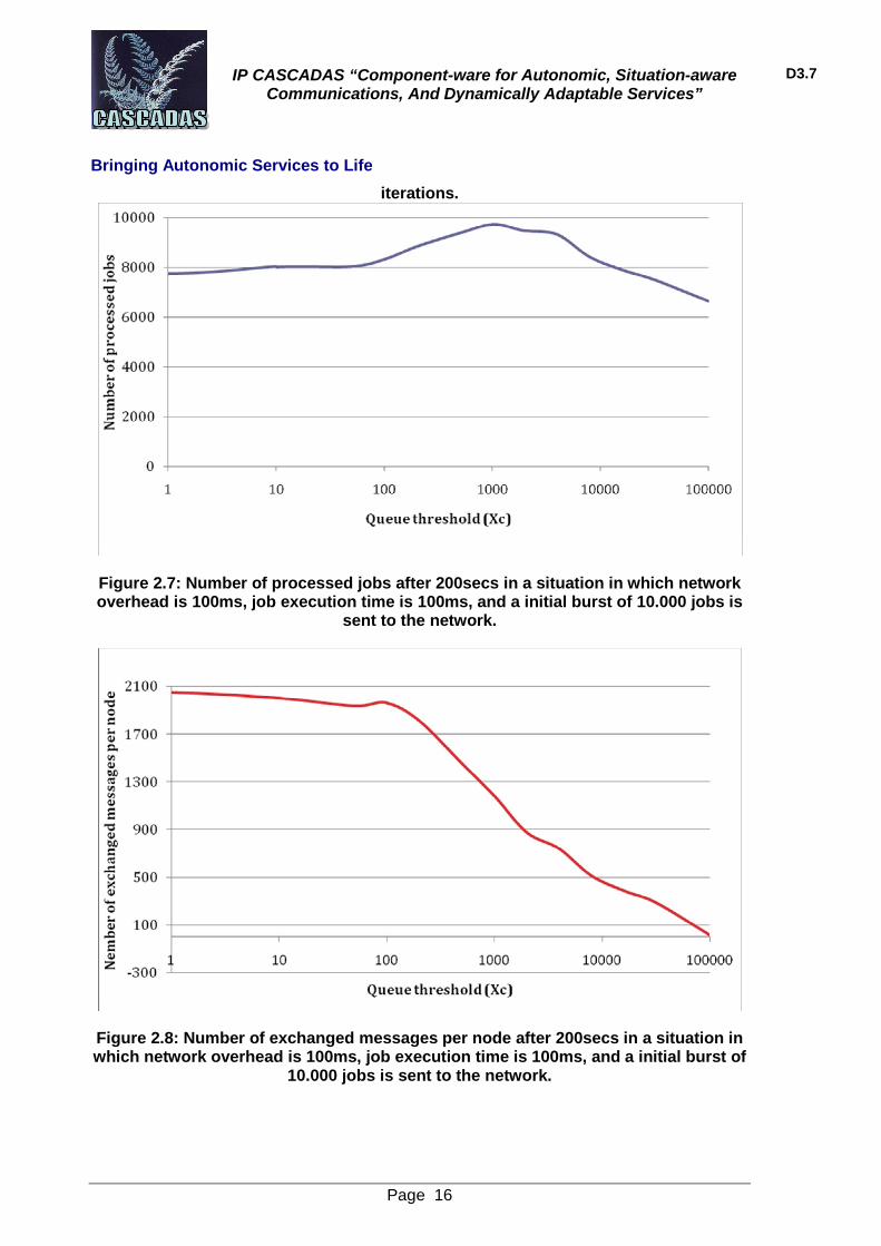
2.3.3 Simulations with medium jobs In this second series of experiments we have a job execution time that is similar to the communication overhead of the network, therefore what we expect is a slightly benefit from rewiring if it occurs with a rate that is not too fast to overload the network with messages, and not too slow to make load-balancing algorithm useless since there would be no spontaneous formation of homogeneous island of worker nodes.
Figure 2.7 shows that there is an optimal value for xc that permits to achieve a maximum number of processed jobs. This result is the most significant one because it includes all the intermediate situations.
IP CASCADAS “Component-ware for Autonomic, Situation-aware Communications, And Dynamically Adaptable Services”
D3.7
Bringing Autonomic Services to Life
Page 16
iterations.
Figure 2.7: Number of processed jobs after 200secs in a situation in which network overhead is 100ms, job execution time is 100ms, and a initial burst of 10.000 jobs is
sent to the network.
Figure 2.8: Number of exchanged messages per node after 200secs in a situation in which network overhead is 100ms, job execution time is 100ms, and a initial burst of
10.000 jobs is sent to the network.

IP CASCADAS “Component-ware for Autonomic, Situation-aware Communications, And Dynamically Adaptable Services”
D3.7
Bringing Autonomic Services to Life
Page 17
2.3.4 Simulations with small jobs This series of simulations has been performed to see if the heuristic is suitable to the case in which jobs are very small. In this situation the time needed to process a job is much lower then the time needed to perform a rewiring iteration or to transfer a job. The expected output is a decrease in network traffic since the queues are consumed in a very fast way and remain very small.
In Figure 2.9 we can see that the number of processed jobs is maximized for infinite values for xc. This means that in this situation the system has limited benefits from the rewiring. However this extreme situation is unlikely to happen in a real network.
Figure 2.9: Number of processed jobs after 35secs in a situation in which network overhead is 100ms, job execution time is 1ms, and a initial burst of 10.000 jobs is
sent to the network.

IP CASCADAS “Component-ware for Autonomic, Situation-aware Communications, And Dynamically Adaptable Services”
D3.7
Bringing Autonomic Services to Life
Page 18
Figure 2.10: Number of processed jobs after 35secs in a situation in which network overhead is 100ms, job execution time is 3ms, and a initial burst of 10.000 jobs is
sent to the network.
2.3.5 Summary In these three classes of experiments we have seen that in the situation in which the network overhead is higher than the execution of the jobs, the choice of performing rewiring iterations simply increases the communication overhead and slows down the execution of the jobs. On the other hand in the opposite situation in which the communication is much lower than the job execution time, an increase in the communication is able to accelerate the algorithm convergence without affecting the capability to execute jobs. Finally in the intermediate situation we can see that there is a value for the threshold of the queue length (xc) that maximizes the total number of completed jobs. Message overhead charts of all the experiments (see Figures 2.6,2.8,2.10) show that an increase of the threshold is able to reduce significantly the network overhead with the side effect of slowing down the rewiring part of the self-adaptive load balancing algorithm.
2.4 Discussion With respect to the state of the art solutions to the load balancing problem (for instance the Dimension Exchange algorithm) the combined approach we have proposed is able to solve it in a wider scope. In particular we have extended the classical solution in the context of dynamic heterogeneous networks without any relevant drawbacks and with comparable performance.
The experiments on the proposed heuristic have shown that using a sigmoid probabilistic function to trigger the execution of the rewiring part of the load balancing algorithm may speed-up the execution of the jobs in situations in which the network overhead is a

IP CASCADAS “Component-ware for Autonomic, Situation-aware Communications, And Dynamically Adaptable Services”
D3.7
Bringing Autonomic Services to Life
Page 19
concern. The results we have obtained may be used to self-adapt the threshold (xc) value by comparing the node service time to the network delay (evaluated – for example – by pinging remote nodes): for high service times the threshold will be gradually decreased to zero to speed-up the node rewirings; if the network latency becomes closer to the node service time, the threshold will be modified to an opportune intermediate value (the exact value for this situation will be the base for a future work); finally if the service time is significantly lower then the network latency, there will be no need for further rewiring and the threshold parameter may grow toward infinite values (thus disabling all rewiring iterations).
Another important point of discussion is the message overhead: in several applications its minimization may be more important than achieving the best value for the number of completed jobs. In such a case the threshold value may be automatically increased until the desired maximum network load is reached, thus finding the best tradeoff between the network overhead and the algorithm performance.
3 Power saving: a use case for self-differentiation
Generally orchestrating the deployment and maintenance of a complex distributed application requiring frequent interactions between its many constituents is a well-identified but difficult and as yet unsolved problem in highly dynamic environments. In recent work, it has been shown that decentralised mechanisms could preside to the emergence of efficient collaborative overlays through self-organised aggregation and to division of labour in a fixed-topology network through co-ordinated individual specialisation [11].
In order for the distributed system to be able to adapt to a change in the overall demand (assuming that the total processing capability is sufficient), it is necessary that resources can be repurposed and re-allocated without a centralized management functionalities in order to obtain self-configuration and scalability.
This “self-(re)allocation” of individual resources, based on locally available information and local interactions, is called “differentiation”, because it shares many characteristics with the eponymous phenomenon in biological morphogenesis [11].
The idea is to analyze how distributed supervision can be realized by applying both self-organization techniques developed in WP3 and exploiting the ACE model developed in WP1 at the maximum extend. We consider the ACE tool-kit embedded supervision applied at two different levels of granularity as a kind of bottom-up process: ACE will be supervised per se by using the self differentiation algorithm and in case of unsuccessful effort the problem could scale to the ACE “neighbors” through the rearrangement of the links; in fact, we could consider the ACE in its role of service provider to be member of (at list) one group of ACEs providing/using the same service.
According to the WP3 definition [11] the differentiation phenomena are that the system (or the individuals) can exist in multiple states among which individuals (or the whole system) can switch. As the ACE behavior both internal (i.e., life cycle) or custom (i.e., the service provided) is represented as a series of states then it’s realistic to think the change of state for an ACE in terms of “(self-) differentiating”.
The use case that will be analyzed in the next sections is about the optimization of energy consumption of Telco and Internet data centres, by minimizing the number of running servers, i.e. maximizing the number of servers in “stand-by” state, and by redistributing the

IP CASCADAS “Component-ware for Autonomic, Situation-aware Communications, And Dynamically Adaptable Services”
D3.7
Bringing Autonomic Services to Life
Page 20
load of tasks to be executed. The approach is aiming at exploiting local interactions (i.e., interactions among neighbours servers in an overlay network) and self-differentiation algorithms. The servers will be represented by ACEs that are organized in an overlay network that interacts between them in order to realize the algorithms for power saving. This could be realised through the ACE toolkit embedded supervision specified in WP2.
3.1 Approach and Algorithm On the base of the self-differentiation behaviour of ACEs the use case will consider:
- a data center as composed by a set of distributed servers (e.g. computing resources), and enforce decentralized energy control (optimisation) solutions to data-centers through self-* algorithms (e.g. differentiation);
- an overlay of ACEs (representing the servers) that enforces load-balancing and status of servers by communicating each other and by running a self-differentiation algorithms;
- ACEs (i.e. servers) are altruistic (they volunteer in taking tasks to free up other servers, that are in a status of very low utilization, and that a such can be enter the stand-by mode).
- According to the amount of load for each ACE, four node states are defined:
o standby: the node does not process any tasks, it’s in energy saving mode. o low load: the node can transfer its load and enter standby mode. o medium load: the node can take further load. o high load: the node cannot take further load.
The two algorithms described here after will be applied to a system which is composed by nodes (ACEs) connected in an overlay network.
Standby Algorithm
The standby algorithm is the algorithm responsible of achieving energy saving. It can be executed by any node (ACE) and by more than one node at the same time. It starts at a random time, when a node (again an ACE) starts acting as a matchmaker [10]. This kind of node, the matchmaker, chooses two random neighbors (two ACEs Node, Node A and B in the following of the text) in the overlay and checks their state. If one of the neighbors is in low load state and the other one is either in low or medium load state it is decided that some energy can be saved. For that purpose, the matchmaker will order the low load node (if they’re both in low load state it doesn’t matter which one is chosen) to transfer its load to the other neighbor. In this way, the node that sent its load goes standby, thus saving some energy.
This algorithm is enough to reduce the power consumption, but it doesn’t take into account the execution time. While there are great results regarding the energy saving, the execution time rockets making the system slow. Thus, another algorithm is necessary to keep reasonable execution time values.
Overload Algorithm
In this second algorithm, each node checks periodically its execution time, which is calculated as the relationship between the number of tasks and the process capability. When this value is over a certain threshold, the node looks for a standby neighbor that can

IP CASCADAS “Component-ware for Autonomic, Situation-aware Communications, And Dynamically Adaptable Services”
D3.7
Bringing Autonomic Services to Life
Page 21
help it lighten its load. The procedure is very similar to the one in the Standby Algorithm, but now the node just selects one neighbor. When the overload node finds a standby neighbor, it transfers half of its load to the neighbor, which wakes up and enters the state corresponding to the load received. By using the Overload Algorithm power saving is reduced, as it wakes standby nodes, but it is necessary otherwise the system would be extremely slow.
For the simulation, Table 1 shows the initial states for nodes (ACEs) A and B and those after the interaction, A’ and B’.
In the Standby Algorithm, there is a third node, the matchmaker, which compares the load of nodes A and B and decides which one and when has to transfer its load.
In the Overload Algorithm the overloaded node (A) contacts directly a standby neighbor (B), without the intervention of a matchmaker.
Standby
A B A’ B’
LL LL ML SB
ML LL ML / HL SB
LL ML SB ML / HL
Overload
A B A’ B’
HL SB ML ML
Table 1: Interaction of nodes in each algorithm
(SB = Standby, LL = Low load, ML = Medium load, HL = high load)
All the classes used in this simulation were developed in JAVA language, as it is the language required by the simulator used: Peersim.
Peersim1 is an open source P2P systems simulator developed by the University of Bologna. The main characteristic of this simulation environment is its modularity, which makes it easy to use.
Peersim creates the overlay according to the number of links (N) set in the configuration file. Every node establishes the indicated number of connections with random nodes (neighbors).
The load in the simulation is distributed as follows:
- low nodes get a random value in the interval [23-33]. - medium nodes get a random value in the interval [56-66]. 1 http://peersim.sourceforge.net/
IP CASCADAS “Component-ware for Autonomic, Situation-aware Communications, And Dynamically Adaptable Services”
D3.7
Bringing Autonomic Services to Life
Page 22
- high nodes get a random value in the interval [89-99]. - if there are any remaining nodes (in the configuration file the sum of the nodes
specified in every state is under 100%), they are initialized with a load of 0 (this doesn’t happen with the random initialization).
Load State Power consumption
0 0 (standby) 5
≤33 1 (low load) 125
>33 and ≤66 2 (medium load) 140
>66 3 (high load) 155
Table 2: State and power consumption assigned depending on the load
There will be presented two approaches, in the first one the incoming load in a cycle is constant, so every cycle has the same amount of load that is set at the beginning. When the algorithms transfer the load from one node to another, the node receiving the load will modify its load value to the sum of its own and that transferred from the neighbor. The other approach explained in the next section will consider a variable load for the nodes.
3.2 Simulation with constant load The parameters of the different simulations analyzed in this section, in order to analyze the simulation results applying a constant load on the nodes, on the base of the simulation environment introduced before, are:
- Number of cycles in the simulation. - Matchmaker threshold: probability for a node to act as a matchmaker. Must be a
value between 0% and 100%. - Matchmaker limit: when a node acts as a matchmaker, it has to wait this number
of cycles until it can be activated as a matchmaker again. Must be a natural number.
- Slow time: when the execution time of the node is over this value, it’s considered to be overloaded. It represents percentage over the initial execution time.
- Normal time: when the execution time of the overloaded node goes below this value, it’s considered to be running normally again. It represents percentage over the initial execution time.
- Load parameters low, medium and high represent the amount of nodes initially in every state. These values must be between 0% and 100%, and the sum of the three of them cannot be greater than 100. If the initial load is set to random, these parameters are not taken into account.
In all cases, the network is composed by 1,000 nodes, with 20 neighbors each and a process capability of tasks/cycle 10. They are initially assigned a random load value between 23 and 33 tasks, corresponding to the low load state. Overload control is local in all the simulations.
When the algorithms are not executed, with all the nodes initially in low load (average load of 28 tasks) and a process capability of tasks/cycle 10 the execution time is 2.8 cycles.

IP CASCADAS “Component-ware for Autonomic, Situation-aware Communications, And Dynamically Adaptable Services”
D3.7
Bringing Autonomic Services to Life
Page 23
All the simulations have been repeated 10 times. After that, the average of the values obtained is calculated: the charts show the results corresponding to that average.
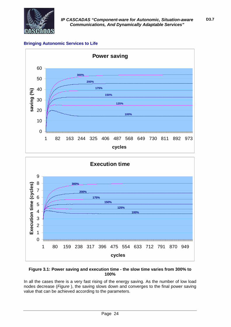
In Experiment 1 all the parameters are fixed but not the slow time, which vary from 300% to 100%. This parameter determines at which point the node decides it is overloaded.
This second simulation observes how results change with different values of the matchmaker threshold, which represents the probability of a node to act as a matchmaker. The range of values goes from 1% to 50%.
The next parameter taken in consideration is the matchmaker limit, in Experiment 3: the number of cycles a node has to wait after acting as a matchmaker before it can do it again.
After those experiments, in Experiment 4 there is a comparison of the maximum saving and execution time values achieved when the initial load of the nodes varies from the situation where all of them are low loaded to that where all of them are high loaded. This initial load distribution can be seen in Figure 3.3.
For this experiment it is used 1,000 cycles, a matchmaker threshold of 5%, a matchmaker limit of 10 and a slow time of 150%. The initial load of the nodes varies from the situation where all the nodes are initially low loaded to that where all the nodes are initially high loaded.
Finally, in Experiment 5 it is offered a comparison on how the results vary depending on the number of neighbors each node has, trying with 2, 3, 4, 5, 10, 15 and 20 links. All the nodes are initially low loaded. The rest of the parameters take the same values as in Experiment 4.
3.2.1 Experiment 1: Different slow time Figure reports the results of the first simulations: all the parameters are fixed but not the slow time, which vary from 300% to 100%. This parameter determines at which point the node decides it is overloaded.
A value of 300% means that the node will consider itself overloaded when its execution time is over 13.2 cycles. With the actual implementation a node will never reach that value, i.e. no overload control is being executed in this simulation. Therefore, the maximum energy saving value is achieved without taking in consideration the execution time.
IP CASCADAS “Component-ware for Autonomic, Situation-aware Communications, And Dynamically Adaptable Services”
D3.7
Bringing Autonomic Services to Life
Page 24
Power saving
0
10
20
30
40
50
60
1 82 163 244 325 406 487 568 649 730 811 892 973
cycles
savi
ng
(%
)
300%
200%
175%
150%
125%
100%
Execution time
0
1
2
3
4
5
6
7
8
9
1 80 159 238 317 396 475 554 633 712 791 870 949
cycles
Exe
cuti
on
tim
e (c
ycle
s) 300%
200%
175%
150%
125%
100%
Figure 3.1: Power saving and execution time - the slow time varies from 300% to 100%
In all the cases there is a very fast rising of the energy saving. As the number of low load nodes decrease (Figure ), the saving slows down and converges to the final power saving value that can be achieved according to the parameters.

IP CASCADAS “Component-ware for Autonomic, Situation-aware Communications, And Dynamically Adaptable Services”
D3.7
Bringing Autonomic Services to Life
Page 25
From the second chart in Figure derives that the execution time has the same behavior described for the power saving.
When overload control is not executed (slow time of 300%) the final saving value is 53.93%, rising over 50% around cycle 150. Unfortunately, the average execution time in the system is also very high, close to 8 cycles.
0%
10%
20%
30%
40%
50%
60%
70%
80%
90%
100%
1 46 91 136 181 22 271 316 361 40 451 49 541 58 631 67
0%
10%
20%
30%
40%
50%
60%
70%
80%
90%
100%
1 40 79 118 157 196 23 27 313 35 391 43 46 50 54 58 62 66
Slow time = 300% Slow time = 200%
0%
10%
20%
30%
40%
50%
60%
70%
80%
90%
100%
1 40 79 118 157 196 23 27 313 35 391 43 46 50 54 58 62 66
0%
10%
20%
30%
40%
50%
60%
70%
80%
90%
100%
1 69 137 205 273 341 409 477 545 613 681 749 817 885 953
Slow time = 175% Slow time = 150%
0%
10%
20%
30%
40%50%
60%
70%
80%
90%
100%
1 89 177 265 353 441 529 617 705 793 881 969
0%
10%
20%
30%
40%
50%
60%
70%
80%
90%
100%
1 89 177 265 353 441 529 617 705 793 881 969
Slow time = 125% Slow time = 100%
Figure 3.2: Percentage of nodes in every state - the slow time from 300% to 100%
Figure shows the evolution of the nodes in every state. If there are a high number of standby nodes there is high savings, but also high execution times, since the rest of the nodes have to execute the tasks that were initially assigned to the standby nodes.
Standby Low Medium High

IP CASCADAS “Component-ware for Autonomic, Situation-aware Communications, And Dynamically Adaptable Services”
D3.7
Bringing Autonomic Services to Life
Page 26
With the slow time set to 300% (no overload control) the maximum number of standby nodes (64.20%) is achieved, getting the maximum saving and also the maximum number of high loaded nodes (28.47%) and the highest execution time.
By reducing the slow time, overload control starts being applied. This results in the reduction of the high loaded nodes is obtained by waking up some standby ones. With this, the execution time decreases, but so does the power saving.
3.2.2 Experiment 2: Different matchmaker threshold This second simulation observes how results change with different values of the matchmaker threshold, which represents the probability of a node to act as a matchmaker. The range of values goes from 1% to 50%.
Since this parameter represents the probability of a node to act as a matchmaker, the final results (once they stabilize) shouldn’t be different from the ones obtained in Experiment 1 when the slow time was 150%.
Power saving
0
5
10
15
20
25
30
35
1 82 163 244 325 406 487 568 649 730 811 892 973
cycles
savi
ng
(%
)
1% 2% 3% 5% 10% 20% 50%

IP CASCADAS “Component-ware for Autonomic, Situation-aware Communications, And Dynamically Adaptable Services”
D3.7
Bringing Autonomic Services to Life
Page 27
Execution time
0
1
2
3
4
5
6
1 76 151 226 301 376 451 526 601 676 751 826 901 976
cycles
1% 2% 3% 5% 10% 20% 50%
Figure 3.3: Power saving and execution time - matchmaker threshold from 1 to 50
Analyzing Figure power saving and execution time have approximately the same values obtained in the previous experiment with a slow time of 150% (saving of 32.66% and execution time of 5 cycles). The only important difference between the different simulations is the time the system needs to converge to the final values. This fact can be seen also in Figure , where the main difference between the different simulations is also the time it takes to reach stability.
0%
10%
20%
30%
40%
50%
60%
70%
80%
90%
100%
1 46 91 136 181 22 271 316 361 40 451 49 541 58 631 67
0%
10%
20%
30%
40%
50%
60%
70%
80%
90%
100%
1 40 79 118 157 196 23 27 313 35 391 43 46 50 54 58 62 66
Matchmaker threshold = 1% Matchmaker threshold = 3%
IP CASCADAS “Component-ware for Autonomic, Situation-aware Communications, And Dynamically Adaptable Services”
D3.7
Bringing Autonomic Services to Life
Page 28
0%
10%
20%
30%
40%
50%
60%
70%
80%
90%
100%
1 69 137 205 273 341 409 477 545 613 681 749 817 885 953
0%
10%
20%
30%
40%50%
60%
70%
80%
90%
100%
1 89 177 265 353 441 529 617 705 793 881 969
Matchmaker threshold = 5% Matchmaker threshold = 10%
0%
10%
20%
30%
40%
50%
60%
70%
80%
90%
100%
1 89 177 265 353 441 529 617 705 793 881 969
0%
10%
20%
30%
40%
50%
60%
70%
80%
90%
100%
1 88 175 262 349 436 523 610 697 784 871 958
Matchmaker threshold = 20% Matchmaker threshold = 50%
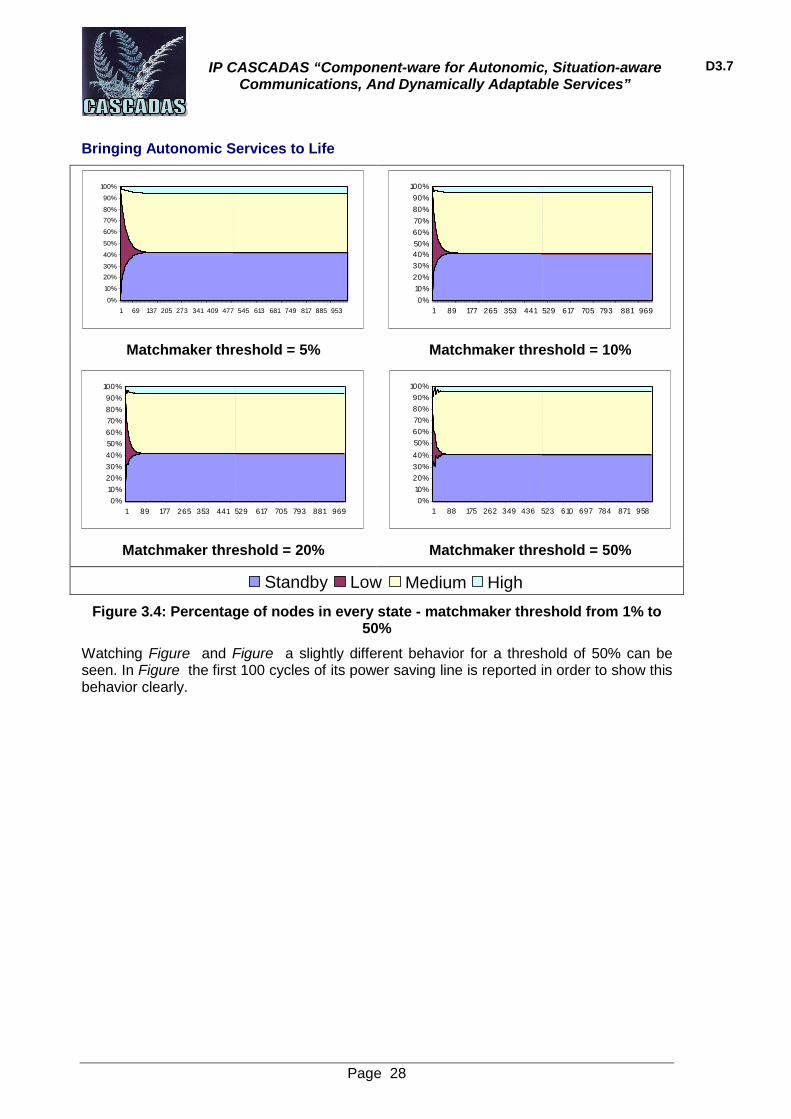
Figure 3.4: Percentage of nodes in every state - matchmaker threshold from 1% to 50%
Watching Figure and Figure a slightly different behavior for a threshold of 50% can be seen. In Figure the first 100 cycles of its power saving line is reported in order to show this behavior clearly.
Standby Low Medium High

IP CASCADAS “Component-ware for Autonomic, Situation-aware Communications, And Dynamically Adaptable Services”
D3.7
Bringing Autonomic Services to Life
Page 29
Power saving
0
5
10
15
20
25
30
35
1 8 15 22 29 36 43 50 57 64 71 78 85 92 99
cycles
savi
ng
(%
)
Figure 3.5: Power saving line corresponding to a matchmaker threshold of 50%
The power saving shows some fluctuations in the beginning. This is because the probability of acting as a matchmaker is so high that huge saving values are obtained in the very beginning, but the execution time also rises very quickly. Then, the Overload Algorithm wakes up the standby nodes necessary to avoid the overload situation, reducing the saving (and the execution time). The number of cycles between each of the peaks shown in the chart depends on the matchmaker limit parameter (in this case 10), as demonstrated in the next simulation.
Since the values are very similar for every value of the matchmaker threshold it is useless to include the chart showing the relationship between power saving and execution time, because it’s clear that the only difference between the lines will be the speed of convergence to the final value (which will be more or less the same in all the cases).
The results will be the same independently of the matchmaker threshold so this value can be chosen freely. However, a higher matchmaker threshold would mean that the nodes act more often as a matchmaker that would entail higher power consumption, even though it is not considered in this model. For this reason, for the next experiments it is chosen a value that’s not too high, like 5%. Anyway, the decision relies again on the specific needs.
3.2.3 Experiment 3: Different matchmaker limit The next parameter taken in consideration is the matchmaker limit: the number of cycles a node has to wait for after acting as a matchmaker before it can do it again. The results, shown in Figure , are very similar as those of Experiment 2, with the same final values but different convergence times.

IP CASCADAS “Component-ware for Autonomic, Situation-aware Communications, And Dynamically Adaptable Services”
D3.7
Bringing Autonomic Services to Life
Page 30
Power saving
0
5
10
15
20
25
30
35
1 82 163 244 325 406 487 568 649 730 811 892 973
cycles
savi
ng
(%
)
0 5 10 20 30 50 100
Execution time
3
3.5
4
4.5
5
5.5
1 78 155 232 309 386 463 540 617 694 771 848 925
cycles
0 5 10 20 30 50 100
Figure 3.6: Power saving and execution time - matchmaker limit varies from 0 to 100
In the analysis of the previous experiment the length of those fluctuations when the threshold was 50% is determined by the value assigned to the limit. In this case, with a threshold of 5% clearly the same happens when the limit is 100 (green line).

IP CASCADAS “Component-ware for Autonomic, Situation-aware Communications, And Dynamically Adaptable Services”
D3.7
Bringing Autonomic Services to Life
Page 31
At the beginning all the nodes can act as a matchmaker, so there’s a fast rising. After this, the nodes have to wait 100 cycles until they can be the matchmaker again. That’s why the value stops rising until the limit is reached, when the Standby Algorithm can be executed again.
This effect can also be seen in the last chart included in Figure , corresponding to the matchmaker limit of 100.
0%
10%
20%
30%
40%
50%
60%
70%
80%
90%
100%
1 46 91 136 181 22 271 316 361 40 451 49 541 58 631 67
0%
10%
20%
30%
40%
50%
60%
70%
80%
90%
100%
1 40 79 118 157 196 23 27 313 35 391 43 46 50 54 58 62 66
Matchmaker limit = 0 Matchmaker limit = 10
0%
10%
20%
30%
40%
50%
60%
70%
80%
90%
100%
1 69 137 205 273 341 409 477 545 613 681 749 817 885 953
0%
10%
20%
30%
40%50%
60%
70%
80%
90%
100%
1 89 177 265 353 441 529 617 705 793 881 969
Matchmaker limit = 20 Matchmaker limit = 30
0%
10%
20%
30%
40%
50%
60%
70%
80%
90%
100%
1 89 177 265 353 441 529 617 705 793 881 969
0%
10%
20%
30%
40%
50%
60%
70%
80%
90%
100%
1 88 175 262 349 436 523 610 697 784 871 958
Matchmaker limit = 50 Matchmaker limit = 100
Figure 3.7: Percentage of nodes in every state - matchmaker limit varies from 0 to 100
Standby Low Medium High

IP CASCADAS “Component-ware for Autonomic, Situation-aware Communications, And Dynamically Adaptable Services”
D3.7
Bringing Autonomic Services to Life
Page 32
3.2.4 Experiment 4: Different initial situations
Figure 3.8: Power saving and execution time with different initial situations
Figure shows the power saving achieved with different initial situations and a slow time set to 150%. The x-axis represents 66 different simulations, each one of them with the initial conditions shown in the upper chart. The middle chart shows the maximum power saving achieved in every case and the lower one, the maximum execution time.
It shows that the maximum saving values are reached in the first cases, when most of the nodes are initially low loaded. This is exactly what is expected, since the algorithm works with the nodes in that state. When there are initially a few or no nodes with low load the energy saving tends to zero.
3.2.5 Experiment 5: Different number of neighbors In Figure the power saving and execution time values obtained are compared when the number of links(N) established by each node changes. The only line separated from the rest is that corresponding to N=2. For the other values of N the results are more or less the same.
This means that there’s almost no difference between having 6 or 40 neighbors. Knowing that, in a real implementation the number of neighbors should be reduced in order to save some resources. In these simulations it is not considered the cost of the creation and maintenance of the overlay, but it’s obviously not the same having 40 neighbors per node than having 6.
0%
20%
40%
60%
80%
100%
1 3 5 7 9 11 13 15 17 19 21 23 25 27 29 31 33 35 37 39 41 43 45 47 49 51 53 55 57 59 61 63 65
Low Medium High
Saving
0
5
10
15
20
25
30
35
40
45
1 3 5 7 9 11 13 15 17 19 21 23 25 27 29 31 33 35 37 39 41 43 45 47 49 51 53 55 57 59 61 63 65
Execution Time
0
2
4
6
8
10
1 3 5 7 9 11 13 15 17 19 21 23 25 27 29 31 33 35 37 39 41 43 45 47 49 51 53 55 57 59 61 63 65

IP CASCADAS “Component-ware for Autonomic, Situation-aware Communications, And Dynamically Adaptable Services”
D3.7
Bringing Autonomic Services to Life
Page 33
Power saving
0
5
10
15
20
25
30
35
1 81 161 241 321 401 481 561 641 721 801 881 961
cycles
savi
ng
(%
)
N = 2 N = 3 N = 4 N = 5 N = 10 N = 15 N = 20
Execution time
2.5
3.0
3.5
4.0
4.5
5.0
1 76 151 226 301 376 451 526 601 676 751 826 901 976
cycles
N = 2 N = 3 N = 4 N = 5 N = 10 N = 15 N = 20
Figure 3.9: Power saving and execution time with different number of links

IP CASCADAS “Component-ware for Autonomic, Situation-aware Communications, And Dynamically Adaptable Services”
D3.7
Bringing Autonomic Services to Life
Page 34
3.2.6 Simulation without matchmaker Finally, some simulations to compare the energy saving and execution time obtained with the role of the matchmaker and without it (the nodes directly contact their neighbors and exchange their load).
Figure shows the charts of Experiment 1 (with the matchmaker) while Figure reports the results obtained without the matchmaker (with the same parameters).
The charts in the two cases are practically equal. Seeing that, it seems logic to choose the second option, since it’s faster and consumes fewer resources.
Power saving
0%
10%
20%
30%
40%
50%
60%
1 64 127 190 253 316 379 442 505 568 631 694 757 820 883 946
cycles
ST=300% ST=200% ST=175% ST=150% ST=125% ST=100%
Execution time
1
2
3
4
5
6
7
8
9
1 66 131 196 261 326 391 456 521 586 651 716 781 846 911 976
cycles
ST=300% ST=200% ST=175% ST=150% ST=125% ST=100%
Figure 3.10: Power saving - execution time with matchmaker (different slow time)

IP CASCADAS “Component-ware for Autonomic, Situation-aware Communications, And Dynamically Adaptable Services”
D3.7
Bringing Autonomic Services to Life
Page 35
Power saving
0
10
20
30
40
50
60
1 70 139 208 277 346 415 484 553 622 691 760 829 898 967
cycles
ST=300% ST=200% ST=175% ST=150% ST=125% ST=100%
Execution time
0123456789
1 63 125 187 249 311 373 435 497 559 621 683 745 807 869 931 993
cycles
ST=300% ST=200% ST=175% ST=150% ST=125% ST=100%
Figure 3.11: Power saving - execution time without matchmaker (different slow time)
3.3 Simulation with load peak The following approach introduces some variations to the previous model according to the studies about utilization of the nodes and traffic model [2].
The main change is in the way the load and the energy consumed by the nodes are modeled. In the previous system, each of the nodes had a value, between 0 and 100, representing the tasks it held, i.e., its load (L). Depending on this value, the state of the

IP CASCADAS “Component-ware for Autonomic, Situation-aware Communications, And Dynamically Adaptable Services”
D3.7
Bringing Autonomic Services to Life
Page 36
node was determined (standby, low, medium or high) and a fixed power consumption value was assigned to each state.
The revised model adds new variables, making it closer to reality. These variables are:
- Number of connections (N): represents the number of active connections in server, i.e. the number of clients currently connected to the node.
- Login rate (LI): in [2], it represents the number of incoming connections per second in a node; but in our model is the number of incoming connections per minute, since every simulation cycle equals to a minute.
- Logout rate (LO): represents the number of disconnections per minute.
With this it is calculated the CPU utilization (U) with the following formula, given in [2]:
The energy consumed (in Watts) by a node will be calculated dynamically from this value with the following formula:
Power = 110 + (15*U)/33 if state != 0
= 5 if state = 0
After the observations on the last part of the previous paragraph, the element of the matchmaker has been eliminated. Now each node interacts directly with a neighbor, reducing to two the number of nodes involved in the process.
The way the load is transferred has changed too. In the first model one node sends its tasks to the other, so the number of tasks in the receiving node was the sum of its own tasks and those of its neighbor.
Now, it is introduced the load transference as the receiving node will get just the login rate of the neighbor (or a part of it) and add it to its own load (L). This way the number of connections is not transferred from one node to the other, since it is not realistic that an already established connection is transferred without logging out from the actual node and logging in to the new one.
In the first model the load was constant through all the simulation. In this new approach, the observations about the variation of the number of connections and the login rate are included in [2]. The idea is to use them as a pattern for the variation of our login and logout parameters. This way the model is more realistic, where L and LO are different depending on the time of the day.

IP CASCADAS “Component-ware for Autonomic, Situation-aware Communications, And Dynamically Adaptable Services”
D3.7
Bringing Autonomic Services to Life
Page 37
0
10
20
30
40
50
60
1 118 235 352 469 586 703 820 937 1054 1171 1288 1405
Minutes
inc.
co
nn
exio
ns/
seco
nd
Login Logout
Figure 3.12: Average login and logout rates throughout a day
Number of connections
0
20000
40000
60000
80000
100000
120000
140000
160000
1 119 237 355 473 591 709 827 945 1063 1181 1299 1417
Minutes
Figure 3.13: Average number of connections throughout a day
The figures above show the average login/logout rates used in this revised model (Figure ) and the resulting number of connections (Figure ). The results shown represent the

IP CASCADAS “Component-ware for Autonomic, Situation-aware Communications, And Dynamically Adaptable Services”
D3.7
Bringing Autonomic Services to Life
Page 38
variation throughout a day, since the simulation time was 1,500 cycles and each cycle stands for a minute (1 day = 1,440 minutes).
Three algorithms take place in every of the nodes. They are very similar to the ones used in the previous model, but introduce some variations.
Standby Algorithm
Quite similar to the Standby Algorithm used in the previous model but with a very big difference: now there is no matchmaker. The matchmaker was removed since it makes no difference and increases power consumption. This way a node with low or medium load will get a random neighbor and check its state. If it is in a low load state, the node executing the algorithm will ask the neighbor to send its load and go to sleep.
Overload Algorithm
This algorithm works in a similar way to the Overload Algorithm used before.
When a node is overloaded it looks for a neighbor that is low loaded so it can transfer part of its load. If the node cannot find any low loaded neighbor, a standby node is waked up to take part of the overloaded node’s load.
This algorithm is slightly different than in the previous model, where the overloaded node always woke up a standby node to help it. By checking the low loaded nodes first it is avoided waking up more nodes than necessary, which helps maintain good saving values.
A node is considered overloaded when it satisfies the following two conditions:
- Its number of connections is over a certain value
- The difference between L and LO is positive.
A negative difference between L and LO means the load of the node is reducing. This could possibly make the node enter the normal range of load. In this way unnecessary exchanges of load that could lead to an increment of the power consumed are avoided.
Underload Algorithm
This algorithm adds a behavior to the first model, opposite to the Overload Algorithm. Its aim is to save some energy by putting to sleep underloaded nodes.
When a node is underloaded it looks for a low or medium loaded neighbor. If that neighbor is found, it will take the load of the underloaded node so it can go standby, thus saving some power.
A node is considered underloaded when it satisfies the following two conditions:
- Its number of connections is below a certain value.
- The difference between L and LO is negative.
The same reasoning used in the Overload Algorithm can be applied to explain the second reason. If the difference between L and LO is positive, the load of the node is increasing. It wouldn’t have sense to transfer its load to a neighbor and go standby because then that neighbor would probably soon become overloaded.
3.3.1 Scheduled simulations The parameters to simulate are the time of a day; the number of cycles set to 1,500 (as stated before, one day has 1,440 minutes, so 1,500 is a good value for this parameter).

IP CASCADAS “Component-ware for Autonomic, Situation-aware Communications, And Dynamically Adaptable Services”
D3.7
Bringing Autonomic Services to Life
Page 39
The matchmaker threshold is set to 5 and the limit to 10: the whole system initially will be in low load, as it is the best performance the model can offer.
In this section two experiments are presented:
- Experiment 1: Fixed number of neighbors (20): analysis of the performance of the model when the number of neighbors is set to 20.
- Experiment 2: Different number of neighbors: comparison of the results obtained with different number of neighbors (2, 3, 4, 5, 10, 15 and 20)
All the simulations have been repeated 20 times, the charts show the average values of those repetitions.
All the parameters with configurable values remain the same, with the exception of process, slow_time and normal_time, which are no longer necessary. Two new parameters are added: low_limit and high_limit: they set the thresholds to determine if the node should go standby or is overloaded.
3.3.2 Experiment 1: Fixed number of neighbors
First of all, a simulation has been done where none of the algorithms is executed in order to get the reference values, corresponding to the state of the nodes and the power consumed by them during a day. The later simulations will compare them to this one to calculate the power saving. There is a fixed number of neighbors, i.e. 20.
Power consumed
80000
90000
100000
110000
120000
130000
140000
1 119 237 355 473 591 709 827 945 1063 1181 1299 1417
Minutes
Figure 3.14: Power consumed by the system throughout a day
Figure shows the power consumed by the system during the different periods of the day: the shape is obviously the same as that in Figure , since the algorithms have not been executed in this simulation.

IP CASCADAS “Component-ware for Autonomic, Situation-aware Communications, And Dynamically Adaptable Services”
D3.7
Bringing Autonomic Services to Life
Page 40
With this as the starting point, the results are improved by introducing the algorithms described before.
To apply these algorithms it’s necessary to set the thresholds low_limit and high_limit. Since the former doesn’t change much the results, it is fixed to 10,000 connections, while four different values are given for the latter: 150,000, 125,000, 100,000 and 80,000 connections.
Number of Connections
0
20000
40000
60000
80000
100000
120000
140000
160000
1 63 125 187 249 311 373 435 497 559 621 683 745 807 869 931 993 1055 1117 1179 1241 1303 1365 1427 1489
No algorithms L 150,000 L 125,000 L 100,000 L 80,000
Figure 3.15: Number of connections in the different simulations
Total Power Consumed
80000
90000
100000
110000
120000
130000
140000
1 55 109 163 217 271 325 379 433 487 541 595 649 703 757 811 865 919 973 1027 1081 1135 1189 1243 1297 1351 1405 1459
No algorithms L 150,000 L 125,000 L 100,000 L 80,000
Figure 3.16: Power consumed in the different simulations
Power Saving
0%
5%
10%
15%
20%
25%
30%
1 61 121 181 241 301 361 421 481 541 601 661 721 781 841 901 961 1021 1081 1141 1201 1261 1321 1381 1441 1501
Saving 150 Saving 125 Saving 100 Saving 80
Figure 3.17: Energy saved in the different simulations

IP CASCADAS “Component-ware for Autonomic, Situation-aware Communications, And Dynamically Adaptable Services”
D3.7
Bringing Autonomic Services to Life
Page 41
Execution time
0
2
4
6
8
10
12
14
16
1 64 127 190 253 316 379 442 505 568 631 694 757 820 883 946 1009 1072 1135 1198 1261 1324 1387 1450
No MM L 150,000 L 125,000 L 100,000 L 80,000
Figure 3.18: Execution time in the different simulations
Figure shows that the number of connections is practically the same through the different simulations, as expected, since the service offered by the system should be the same as in the first situation. Therefore, this chart is not of special interest, but it is helpful to analyze Figure , Figure and Figure .
Figure shows the power consumption by the whole system in the different simulations, depending on the value given to high_limit. In Figure the power saving achieved in the different simulations is presented: a bigger limit gets better saving values, but this means there are more high loaded nodes, since they don’t consider themselves overloaded until the limit is reached. This fact can be seen on Figure , where the percentage of nodes in each of the states throughout the day is shown: as high_limit decreases and a better distribution of the load is obtained, so the execution time also decreases (shown in Figure ).
0%
20%
40%
60%
80%
100%
1 49 97 145 193 241 289 337 385 433 481 529 577 625 673 721 769 817 865 913 961 1009 1057 1105 1153 1201 1249 1297 1345 1393 1441 1489
Standby Low Medium High
0%
20%
40%
60%
80%
100%
1 49 97 145 193 241 289 337 385 433 481 529 577 625 673 721 769 817 865 913 961 1009 1057 1105 1153 1201 1249 1297 1345 1393 1441 1489
0%
20%
40%
60%
80%
100%
1 49 97 145 193 241 289 337 385 433 481 529 577 625 673 721 769 817 865 913 961 1009 1057 1105 1153 1201 1249 1297 1345 1393 1441 1489

IP CASCADAS “Component-ware for Autonomic, Situation-aware Communications, And Dynamically Adaptable Services”
D3.7
Bringing Autonomic Services to Life
Page 42
0%
20%
40%
60%
80%
100%
1 49 97 145 193 241 289 337 385 433 481 529 577 625 673 721 769 817 865 913 961 1009 1057 1105 1153 1201 1249 1297 1345 1393 1441 1489
0%
20%
40%
60%
80%
100%
1 49 97 145 193 241 289 337 385 433 481 529 577 625 673 721 769 817 865 913 961 1009 1057 1105 1153 1201 1249 1297 1345 1393 1441 1489
Standby Low Medium High
Figure 3.19: Percentage of nodes in every state in the different simulations: a) No algorithms / b) high_limit: 150,000 / c) high_limit: 125,000 / d) high_limit: 100,000 / e)
high_limit: 80,000
Taking the total power consumed by the system in the different scenarios and comparing it with the consumption when the system is running without any additional algorithms, the total saving values are obtained. Table 3 shows this percentage of energy that can be saved in a day, along with the average execution time.
high_limit Total saving Average execution time
150,000 11.66% 11.04 cycles
125,000 10.07% 10.09 cycles
100,000 8.23% 9.33 cycles
80,000 7.03% 8.83 cycles
Table 3: Percentage of energy saved depending on the value of high_limit
3.3.3 Experiment 2: Different number of neighbors This experiment presents the number of neighbors with a high_limit of 100,000 connections.
In this case is impossible to see any differences in the charts showing the values throughout the day, so it has been decided to introduce charts with the average values in a day for the different number of links.
In Figure the power saving doesn’t change much by changing the number of neighbors: 7.86% is the minimum value (when N=2) and 8.98% is the maximum (when N=10). In Figure the execution time doesn’t change much either, from the maximum value 9.72 cycles (N=10) to 9.31 (N=20). For both cases, the variations are not very important.

IP CASCADAS “Component-ware for Autonomic, Situation-aware Communications, And Dynamically Adaptable Services”
D3.7
Bringing Autonomic Services to Life
Page 43
Power saving
0%1%2%3%4%5%6%7%8%9%
10%
N = 2 N = 3 N = 4 N = 5 N = 7 N = 10 N = 12 N = 15 N = 17 N = 20
Figure 3.20: Power saving with different number of links
Execution time
0
2
4
6
8
10
12
N = 2 N = 3 N = 4 N = 5 N = 7 N = 10 N = 12 N = 15 N = 17 N = 20
Figure 3.21: Execution time with different number of links
3.4 Final Remarks Through the simulation results the performance of the different simulated models, depending on the variation of a set of parameters has been reported. Firstly, the evaluation of the behavior of the system with a flat load level is presented and after that the performance of the system with a more realistic load shape. In the case of the distributed data center, this realistic traffic corresponds to the one presented in [2]. Important saving values are achievable (around 10% and over) with the application of the simple algorithms described.

IP CASCADAS “Component-ware for Autonomic, Situation-aware Communications, And Dynamically Adaptable Services”
D3.7
Bringing Autonomic Services to Life
Page 44
The work presented in this document shows that it's possible to achieve important saving values in distributed data centers, while preserving reasonable execution times, by the introduction of simple algorithms that are executed at a local level. The higher the saving is the higher the execution time gets, so in any case the administrator of the system will have to set the parameters of the model according to the performance expected.
4 Collective decision-making for supervision
4.1 Problem Description An interesting case of collective decision-making involves situations in which different stakeholders might have different appreciations of the quality or attractiveness of a given option. This could be either because of an intrinsic difficulty in obtaining (and/or communicating) a precise measurement of the quality of a solution, or because the perceived quality is a function of some internal variable(s), the value of which can vary from one measuring entity to the other. Interestingly, both sources of noise often combine in natural systems [6].
A concrete case of such a situation can be found in collective supervision. We envisage a situation involving a number of autonomous and selfish supervisors, each of which has exclusive control over a resource (i.e. supervisor = resource controller). For simplicity, we will assume that the resource is a physical host and that there is an exclusive subordination relationship between resident functional ACEs (encapsulations of a service) and their local supervisor. In this scenario, the role of the supervisor amounts to controlling the migration of ACEs so as to ensure that the local population meets some target criterion. Because of the exclusive hierarchical relationships, this typically requires supervisors to exchange ACEs, which in turn requires the ability to reach a consensus. Indeed, initiating the migration of a specific ACE (i.e. handing over its supervision) must be perceived as beneficial to both resource controllers.
In order to increase the clarity of the demonstration, we hypothesise that the number of services (types of functional ACEs) is identical to the number of hosts, and that there is an advantage in aggregating all ACEs of the same type in a given location. This could easily be justified by the ability to fine tune local resources so as to optimise the performance of a specific service once a host is fully “specialised” (i.e. when all resident ACEs belong to a single functional type).
The difficulty is to ensure convergence towards a single global configuration (mapping of services to hosts) that all supervisors agree upon and that can be reached at the lowest possible cost and/or after the shortest possible delay. For instance, if there are three services (labeled “A”, “B” and “C”), all represented by a population of the corresponding functional ACEs, then there are already 6 valid global configurations: ABC, ACB, BAC, CAB, BCA and CBA. However, the initial distribution of ACEs can make one of these “cheaper” to achieve, e.g. because it will involve fewer migrations. Furthermore, the transition cost can be different for each supervisor and two solutions that are equally good for one of them can have substantial advantages or disadvantages for its counterparts.
Let us consider for instance a situation in which there are 8 ACEs of each type and the initial distribution involve, for host 1, 4A, 2B, 2C, for host 2, 2A, 4B, 2C and for host 3, 2A, 2B, 4C… Then from host 1’s point of view, ABC and ACB are equally desirable
IP CASCADAS “Component-ware for Autonomic, Situation-aware Communications, And Dynamically Adaptable Services”
D3.7
Bringing Autonomic Services to Life
Page 45
configurations (both would only involve 8 migrations, whilst any other would involve 12), but for B and C, ABC is the better one. How can we promote the selection of ABC by all three supervisors without having to conduct an explicit evaluation of all possible configurations at system level?
4.2 Decision algorithm To achieve this goal, a modified version of the decision algorithm presented in D3.5 was developed. Fundamentally, supervisors behave like scouts in the sense that they can:
· evaluate the quality of a configuration (based exclusively on local information, i.e. the current population of resident ACEs)
· “compare notes” with other supervisors in an attempt to identify a mutually acceptable configuration (or compromise)
Whenever it decides (with a fixed probability) to evaluate an alternative, randomly generated configuration to its current favourite, its quality is calculated based on the composition of the resident population:
)(icjX
xQ j
ci
=
=
Where j = c(i) is the specialisation of host i in configuration c, xj is the current number of resident ACEs of type j and X is the total number of local ACEs. So, obviously, the quality Q will vary between 0 (when there are no resident ACEs of the type corresponding to the specialisation of the host in the configuration under evaluation) and 1 (when the host is already fully specialised and only ACEs of the correct type are supervised by the local resource controller). For example, if host i has 10 ACEs, and 3 of them are of type “A”, then quality of configuration c for host i (Qci) in which it is specialized in type ”A” (j=c(i)=”A”) would be 0.3.
A configuration that doesn’t contain a specialist for every service (i.e., in our case, any configuration that has two or more specialists of the same type) is automatically given a value of zero. So in effect, the vast majority of combinations (nn-n! if there are n types) have a zero probability of being selected, even though they can be submitted for evaluation by the random generator.
Changing preferences is done as per the equation given in D3.5:
hh
h
*
*
icci
cicc QQ
QP
+=®
However, the rule for comparing solutions between supervisors is now deterministic and simpler than in the original decision-making algorithm. Basically, whenever there is an interaction between two scouts (fixed probability), they both adopt one of their respective preferred configurations as their common favourite. The chosen solution is the one that has the highest value to the other party, so ci*, the preferred configuration of scout i, will become the favourite of scout j as well if:

IP CASCADAS “Component-ware for Autonomic, Situation-aware Communications, And Dynamically Adaptable Services”
D3.7
Bringing Autonomic Services to Life
Page 46
icjc jiQQ ** >
And vice-versa. In the unlikely event that both solutions are equal, one is selected at random. For example, scout i meets scout j, scout i has preferred configuration ci and scout
j has preferred configuration cj. Then if quality of ci is better for scout j than quality of cj is
for scout i, the configuration ci is chosen by both scouts.
In addition to a reference to its preferred configuration, each supervisor also maintains a “confidence index”. This index is incremented by one unit every time that the currently favoured configuration ends up “victorious” from a confrontation (either with another randomly generated configuration or with the preferred option of another supervisor). Conversely, the confidence index of a supervisor whose preferred configuration has just changed is reset to zero (similar to the generic model described in D3.5).
The confidence index is also used to determine when migration actually occurs. Basically, every time that two supervisors find that they already share the same preferred configuration, they also check that both their confidence indexes are above a predefined threshold (in our numerical experiments, this threshold is set to 10n, with n the number of services/hosts). If this is the case, whenever possible, i.e. if a supervisor still hosts at least one ACE of the type in which its counterpart is specialising under their common favourite configuration, up to two ACEs (one in each direction) migrate between them.
4.3 Numerical experiments In order to test the decision algorithm described in the previous section, we ran a set of numerical experiments using an extension of the simulation engine developed by WP3 over the whole duration of the project. We chose not to build an ACE-based version because we needed to run a very large number of experiments in order to obtain enough data for analysis and the overhead resulting from using the ACE tool-kit made that option impractical. See section 5 for a detailed example of how to implement collective decision-making self-models compatible with the tool-kit.
4.3.1 Random initial conditions: In one set of experiments, we start with the whole population of ACEs (32 for each type) randomly distributed among the n hosts (reminder: the local resource controller is de facto the supervisor of all resident ACEs). This means that, if a valid configuration (i.e. featuring one specialist of each type) is chosen at random and arbitrarily set as the global target, a fraction of (n-1)/n resident ACEs will statistically have to “emigrate” from each host. In total, if n=4 for instance, that represents an average 96 migrations. Yet because of random fluctuations, some hosts may have more residents from one type than from any other. Accordingly, a solution in which this host is specialised into that particular type will be more attractive to the local resource controller.
However, there may be conflicts: for instance one initial configuration may have two different hosts biased in favour of becoming specialists of the same service type, which, in our chosen scenario, would be an invalid configuration. The ability of the supervisors to collectively resolve such conflicts and converge towards selecting an option that minimises the overall number of migrations is the key to system efficiency. In other words, if

IP CASCADAS “Component-ware for Autonomic, Situation-aware Communications, And Dynamically Adaptable Services”
D3.7
Bringing Autonomic Services to Life
Page 47
successful, we should observe that, statistically, the total number of migrations is smaller than if a target configuration had been chosen at random and imposed to all supervisors.
This is indeed the case, as illustrated by Figure 4.1, which shows the number of migrations for Pexp=0.75 in all three tested system sizes (n=4, 5 and 6). For all runs, the stop condition is that every site is fully specialised in its assigned type, according to the corresponding supervisor’s favourite system configuration. This means that it only hosts the correct functional ACEs, which implies that all of them are co-located since, in our scenario, there can only be one specialist of every type.
It can clearly be seen that the average number of migrations falls consistently below the “expected” value (96, 128 and 160 for n=4, 5 and 6 respectively), though in some rare cases, the collective decision process completely fails, resulting in many unnecessary adjustments (repeated migrations, see maximum observed values). Note that there are nn possible configurations out of which n! are valid, so this is not an easy problem to solve as soon as there are more than a handful of types/hosts. For instance, with n=6, there are already 46656 options and 720 viable solutions.
0.55
0.7
0.85
1
1.15
1.3
1.45
n=4 n=5 n=6
Number of types (sites)
Mig
rati
on
s (o
bse
rved
/"ex
pec
ted
")
Average
Figure 4.1: Efficiency of the collective selection of a global configuration, in the case where all ACEs (32 of each type) are randomly distributed in initial conditions. Error
bars indicate minimum and maximum values observed over 100 runs.
The quality of the solution (inversely proportional to the number of migrations used to reach it) is only one of the relevant variables though. As could be expected, there appears to be a trade-off between the quality of a consensus and the average number of interactions needed before a clear-cut decision emerges. As can be seen from Figure 4.2, for higher exploration rate (Pexp), this number goes up extremely fast (note that the Y axis is in logarithmic scale). Furthermore, this effect appears to be more pronounced for lower

IP CASCADAS “Component-ware for Autonomic, Situation-aware Communications, And Dynamically Adaptable Services”
D3.7
Bringing Autonomic Services to Life
Page 48
diversity (number of types), which may seem counter-intuitive. It can however be explained by the fact that, for higher values of n, valid solutions represent a proportionally smaller fraction of all possible configurations, thereby limiting the number of explorations leading to a supervisor’s “change of mind”. This effect indirectly favours the emergence of a consensus, hence the faster decision for higher values of n and identical exploration rate (the number of interactions between supervisors being proportional to 1-Pexp, a linear relationship between this number and the time to completion can be expected).
1.E+02
1.E+03
1.E+04
1.E+05
1.E+06
1.E+07
0.45 0.55 0.65 0.75 0.85 0.95
Pexp
Inte
ract
ion
s
4 Types5 Types6 Types
Figure 4.2: Influence of the exploration probability Pexp on the speed of the decision-making process (values averaged over 100 numerical experiments per point). See
text for details.
The two points that are out of alignment in the 6 types scenario (corresponding to Pexp<0.6) correspond to a pathological case, as further evidenced by a similar disruption in the average number of migrations observed for these values (see Figure 4.3). In fact, for Pexp=0.5, n=6, we observe a huge variability, with the number of migrations varying between extremes of 142 and 11211, i.e. an interval spanning two orders of magnitude. Whilst the low value is close to the expected 160 relocations, the high one was observed in a situation where many ACEs had to move repeatedly between hosts as the preferred configuration kept changing. This seems to be the result of a consensus emerging before the reduced exploration probability had allowed for an adequate sampling of the whole configuration space. Subsequent discovery of more attractive solutions led to successive reorganisations, as supervisors changed preference after having reached the confidence
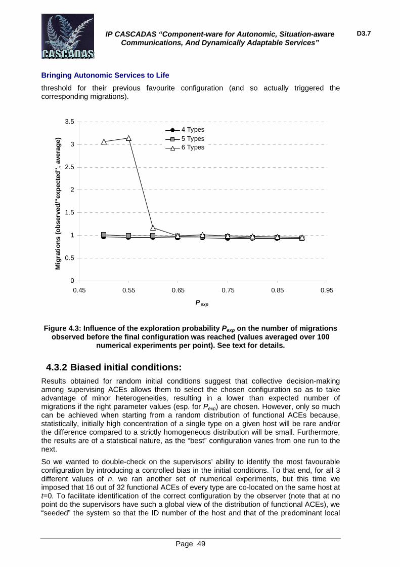
IP CASCADAS “Component-ware for Autonomic, Situation-aware Communications, And Dynamically Adaptable Services”
D3.7
Bringing Autonomic Services to Life
Page 49
threshold for their previous favourite configuration (and so actually triggered the corresponding migrations).
0
0.5
1
1.5
2
2.5
3
3.5
0.45 0.55 0.65 0.75 0.85 0.95
Pexp
Mig
rati
on
s (o
bse
rved
/"ex
pec
ted
", a
vera
ge)
4 Types5 Types6 Types
Figure 4.3: Influence of the exploration probability Pexp on the number of migrations observed before the final configuration was reached (values averaged over 100
numerical experiments per point). See text for details.
4.3.2 Biased initial conditions: Results obtained for random initial conditions suggest that collective decision-making among supervising ACEs allows them to select the chosen configuration so as to take advantage of minor heterogeneities, resulting in a lower than expected number of migrations if the right parameter values (esp. for Pexp) are chosen. However, only so much can be achieved when starting from a random distribution of functional ACEs because, statistically, initially high concentration of a single type on a given host will be rare and/or the difference compared to a strictly homogeneous distribution will be small. Furthermore, the results are of a statistical nature, as the “best” configuration varies from one run to the next.
So we wanted to double-check on the supervisors’ ability to identify the most favourable configuration by introducing a controlled bias in the initial conditions. To that end, for all 3 different values of n, we ran another set of numerical experiments, but this time we imposed that 16 out of 32 functional ACEs of every type are co-located on the same host at t=0. To facilitate identification of the correct configuration by the observer (note that at no point do the supervisors have such a global view of the distribution of functional ACEs), we “seeded” the system so that the ID number of the host and that of the predominant local
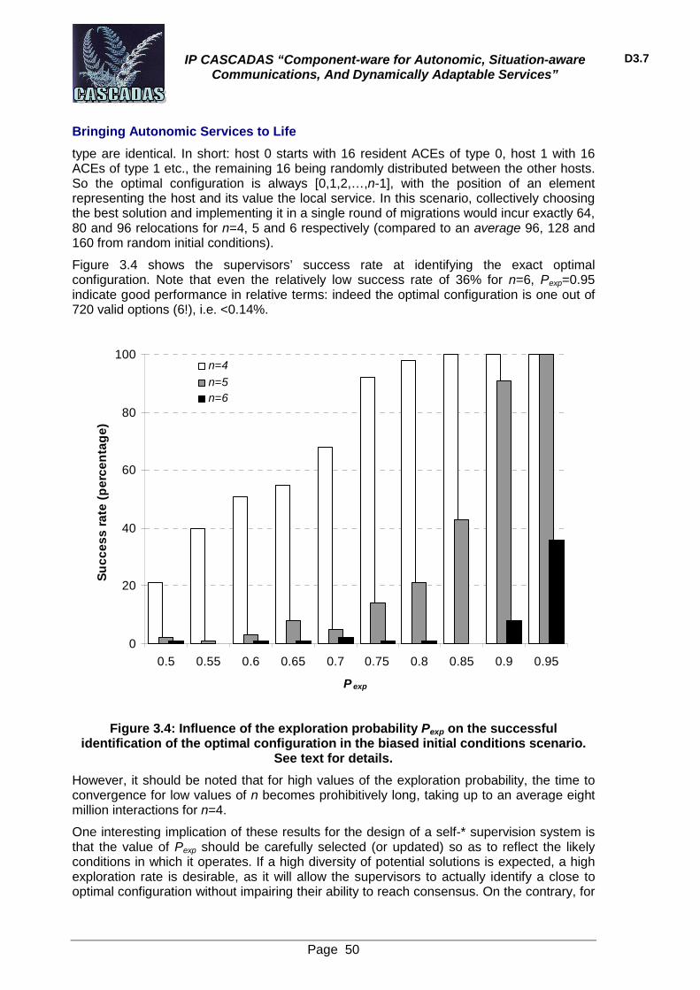
IP CASCADAS “Component-ware for Autonomic, Situation-aware Communications, And Dynamically Adaptable Services”
D3.7
Bringing Autonomic Services to Life
Page 50
type are identical. In short: host 0 starts with 16 resident ACEs of type 0, host 1 with 16 ACEs of type 1 etc., the remaining 16 being randomly distributed between the other hosts. So the optimal configuration is always [0,1,2,…,n-1], with the position of an element representing the host and its value the local service. In this scenario, collectively choosing the best solution and implementing it in a single round of migrations would incur exactly 64, 80 and 96 relocations for n=4, 5 and 6 respectively (compared to an average 96, 128 and 160 from random initial conditions).
Figure 3.4 shows the supervisors’ success rate at identifying the exact optimal configuration. Note that even the relatively low success rate of 36% for n=6, Pexp=0.95 indicate good performance in relative terms: indeed the optimal configuration is one out of 720 valid options (6!), i.e. <0.14%.
0
20
40
60
80
100
0.5 0.55 0.6 0.65 0.7 0.75 0.8 0.85 0.9 0.95
P exp
Su
cces
s ra
te (
per
cen
tag
e)
n=4
n=5n=6
Figure 3.4: Influence of the exploration probability Pexp on the successful identification of the optimal configuration in the biased initial conditions scenario.
See text for details.
However, it should be noted that for high values of the exploration probability, the time to convergence for low values of n becomes prohibitively long, taking up to an average eight million interactions for n=4.
One interesting implication of these results for the design of a self-* supervision system is that the value of Pexp should be carefully selected (or updated) so as to reflect the likely conditions in which it operates. If a high diversity of potential solutions is expected, a high exploration rate is desirable, as it will allow the supervisors to actually identify a close to optimal configuration without impairing their ability to reach consensus. On the contrary, for
IP CASCADAS “Component-ware for Autonomic, Situation-aware Communications, And Dynamically Adaptable Services”
D3.7
Bringing Autonomic Services to Life
Page 51
relatively small “configuration spaces” (as in the n=4 case), Pexp should be kept relatively low, as repeated swapping between equally attractive options (from an individual supervisor’s point of view) has a paralysing effect on collective behaviour. Ideally, the fact that this effect is more pronounced when biased conditions are encountered (i.e. when relative attractiveness of alternative solutions varies more widely) should also be taken into account. In the future, we anticipate that a second layer of “reasoning capabilities” allowing decision-making units to detect and avoid pathological regimes might offer the most robust solution. Such capabilities could simply take the form of the probability of “changing one’s mind” decreasing as a function of how many such decisions have already been made over some predetermined time-window (similar to what we’ve proposed in previous work, see [8]). However, we ran out of time to experiment with this option for the purpose of this deliverable.
5 Collective decision-making for ACE migration
5.1 Introduction In this part of the deliverable we describe the implementation of the collective decision based migration algorithm developed within WP3 (algorithm’s implementation in simulation has been described in D3.5.) with ACE Toolkit. This section also provides guidelines for integrating the algorithm into other applications.
5.2 Algorithm description This section gives brief description of the algorithm. For more detailed description please refer to D3.5.
Agent population is deployed on a number of hosting sites divided into two groups: scouts and workers. The main goal of scout is to gather information about different hosting sites and decide which one it prefers. Also scouts can compare site information between each other and convince other scouts that their site is better. The main goal of worker is to provide the actual service of the application (e.g. perform calculations, etc.). Workers periodically contact random scouts which provide them with their hosting site preference. After the certain number of scouts in a row provides the same site as preferred – worker migrates to that site.
The resulting dynamics of the system are such that when most of the scouts ‘agree’ on one particular site – all workers migrate to that site. If scouts cannot reach the ‘agreement’ – workers do not migrate.
5.3 Implementation in ACE Toolkit The algorithm implementation in ACE Toolkit is very similar to the original algorithm description – it contains scout and worker ACEs. However one more type of ACE is introduced – hosting site monitor (monitor). ACE descriptions are as follows:
Scout ACE – scout ACEs reside anywhere in the network and periodically contact monitors and other scouts to update their site preference. Also scouts provide their site preference to the worker ACEs. Scouts do not migrate. Scouts have one contract between themselves

IP CASCADAS “Component-ware for Autonomic, Situation-aware Communications, And Dynamically Adaptable Services”
D3.7
Bringing Autonomic Services to Life
Page 52
called “scouting contract” which they use to communicate between each other. Each scout also has one contract with monitor ACEs called “monitoring contract” which they use for contacting monitors for site information.
Worker ACE – worker ACEs are deployed anywhere in the network. They contact scout ACEs periodically to record scouts site preference. If the migration threshold (the number of scouts in a row who have the same site preference) is reached worker migrates to the specified site. Each worker has one contract with a number of scouts. The worker ACE self-model can be embedded into other ACE as common-behaviour in order to provide automatic migration based on information provided by the scouts.
Monitor ACE – monitor ACE is located in every hosting site on the network. It gathers the information about its site and provides it to the scouts when they request it.
5.4 ACE self-models In this section we present self-models of the ACEs:
5.4.1 Scout ACE Scout ACE’s self model execution is as follows:
The “INITIAL PLAN” is started - it establishes the “scouting contract” and “monitoring contract” for the scout. Then it starts “WORKER REPLY PLAN” (WRP), “SCOUT REPLY PLAN” (SRP) and “MAIN PLAN” (MP) which will run in parallel. WRP replies to worker requests – sends information of its preferred site when requested. SRP replies to request made by other scouts – sends site information and also compares the site information provided by another scout with its current site and changes its preferred site if necessary. MP periodically contacts other scouts or hosting sites (the decision on who to contact is made probabilistically based on exploration rate) and updates its site preference if necessary. Also each scout uses “ga-reply-behavior” common behaviour which simply sends GA when GN for ‘scouting’ is received. State machines representing scouts plans are shown below.
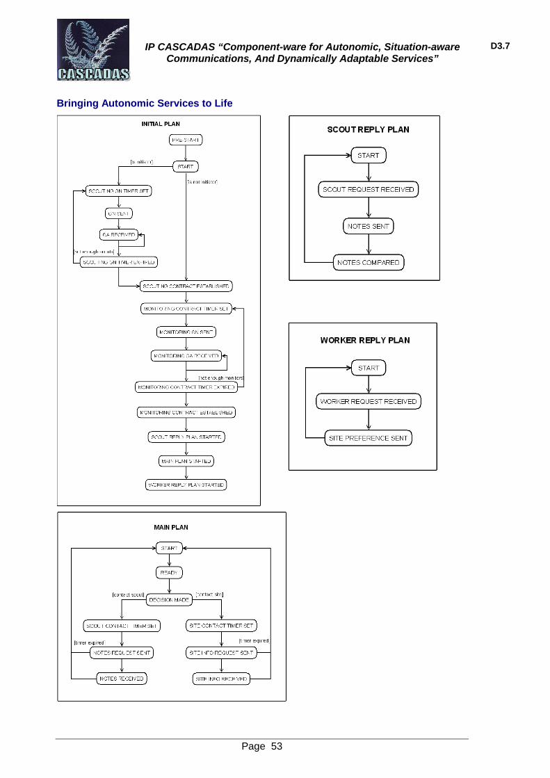
IP CASCADAS “Component-ware for Autonomic, Situation-aware Communications, And Dynamically Adaptable Services”
D3.7
Bringing Autonomic Services to Life
Page 53
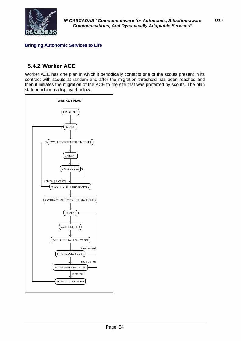
IP CASCADAS “Component-ware for Autonomic, Situation-aware Communications, And Dynamically Adaptable Services”
D3.7
Bringing Autonomic Services to Life
Page 54
5.4.2 Worker ACE Worker ACE has one plan in which it periodically contacts one of the scouts present in its contract with scouts at random and after the migration threshold has been reached and then it initiates the migration of the ACE to the site that was preferred by scouts. The plan state machine is displayed below.
IP CASCADAS “Component-ware for Autonomic, Situation-aware Communications, And Dynamically Adaptable Services”
D3.7
Bringing Autonomic Services to Life
Page 55
5.4.3 Monitor ACE Monitor ACE has one plan which just responds to the request for information about the site that it is hosted in. Also monitor ACE uses the “ga-reply-behavior” common behaviour to reply with GA to the monitoring GN messages. The monitor ACE plan is show below.
5.5 ACE parameters ACE parameters allow customizing the behaviour of the ACE without need to modify code. This section explains the parameters that have to be defined for ACEs.
5.5.1 Scout ACE Parameter name Type Description
INITIAL_WAIT java.lang.String The time in milliseconds for ACE to wait between pre-start and start states in INITIAL PLAN.
INITIATOR java.lang.String
If the value is set to “true” that means this scout will initiate the scouting contract establishment. It is recommended that only small fraction of scouts (preferably one) would have this parameter set to “true”.
SCOUTS_THRESHOLD java.lang.Integer
The minimum number of scouts in a “scouting contract”. Until this number is reached scout will keep sending GN messages. Only used if INITIATOR is “true”.
SCOUTING_GN_TIMER java.lang.String
The interval in ms of wait after sending GN message until the “scouting contract” establishment attempt is made.
MONITORING_CONTRACT_TIMER java.lang.String The interval in ms of wait after sending GN message until the “monitoring contract”

IP CASCADAS “Component-ware for Autonomic, Situation-aware Communications, And Dynamically Adaptable Services”
D3.7
Bringing Autonomic Services to Life
Page 56
establishment attempt is made.
MONITORS_THRESHOLD java.lang.Integer
The minimum number of monitors in a “monitoring contract”. Until this number is reached scout will keep sending GN messages.
SCOUTING_INTERVAL java.lang.String
The time in ms the scout will wait before making the decision whether to contact scout or monitor.
SCOUT_CONTACT_TIMER java.lang.String
The time in ms the scout will wait after sending information request to another scout before discarding the operation.
SITE_CONTACT_TIMER java.lang.String
The time in ms the scout will wait after sending information request to monitor before discarding the operation.
PARAM_ETA java.lang.Double η parameter from equation framework (see D3.5 section 3.1.2 fror details)
PARAM_LAMBDA java.lang.Double λ parameter from equation framework (see D3.5 section 3.1.4 fror details)
PARAM_GAMMA java.lang.Double γ parameter from equation framework (see D3.5 section 3.1.4 fror details)
EXPLORATION_PROBABILITY java.lang.Double
The probability that scout will decide to contact monitor for information as opposed to contacting scout.
GA_REPLY_GOAL_NAME java.lang.String The parameter of “ga-reply-behavior” common behaviour. Has to be set to “SCOUTING”
GA_REPLY_SERVICE_NAME java.lang.String The parameter of “ga-reply-behavior” common behaviour. Has to be set to “SCOUTING”
5.5.2 Worker ACE Parameter name Type Description
INITIAL_WAIT java.lang.String The time in milliseconds for ACE to wait between pre-start and start states.
MINIMUM_NUMBER_OF_SCOUTS java.lang.Integer Minimum number of scouts worker has to recruit before it

IP CASCADAS “Component-ware for Autonomic, Situation-aware Communications, And Dynamically Adaptable Services”
D3.7
Bringing Autonomic Services to Life
Page 57
start execution.
SCOUT_RECRUITMENT_TIMER java.lang.String
The time in ms the worker will wait after sending GN for scouts before attempting to establish contract with scouts.
SCOUT_CONTACT_INTERVAL java.lang.String The time in ms defines the rate at which the worker will be contacting scouts.
SCOUT_CONTACT_TIMER java.lang.String
The time in ms the worker will wait after sending information request to scout before discarding the operation.
MIGRATION_THRESHOLD java.lang.Integer
The number of scouts with the same site preference the scout has contacted in a row in order to trigger migration.
5.5.3 Monitor ACE Parameter name Type Description
SITE_ID java.lang.Integer This parameter is implementation specific used only in our implementation of monitor ACE.
GA_REPLY_GOAL_NAME java.lang.String The parameter of “ga-reply-behavior” common behaviour. Has to be set to “MONITORING”
GA_REPLY_SERVICE_NAME java.lang.String The parameter of “ga-reply-behavior” common behaviour. Has to be set to “MONITORING”
5.6 Experiments A number of experiments have been performed to test behavior of the algorithms implementation using ACE Toolkit.
5.6.1 Experimental setup All experiments were run on a distributed system consisting of 3 machines interconnected with LAN. REDS broker server runs on one of the machines. The initial ACE allocation in the system is as follows: 3 monitor ACEs (one per machine), 4 scout ACEs (located in a single machine), 9 worker ACEs (3 per machine).
5.6.2 Experiment runs ACE parameters used in the experiments were the following:

IP CASCADAS “Component-ware for Autonomic, Situation-aware Communications, And Dynamically Adaptable Services”
D3.7
Bringing Autonomic Services to Life
Page 58
Scout ACEs:
Parameter name Value
INITIAL_WAIT 0
SCOUTS_THRESHOLD 4
SCOUTING_GN_TIMER 2000ms
MONITORING_CONTRACT_TIMER 2000ms
MONITORS_THRESHOLD 3
SCOUTING_INTERVAL 1000ms
SCOUT_CONTACT_TIMER 2000ms
SITE_CONTACT_TIMER 2000ms
PARAM_ETA 2
PARAM_LAMBDA 2
PARAM_GAMMA 2
EXPLORATION_PROBABILITY 0.1
Worker ACEs:
Parameter name Value
INITIAL_WAIT 1000ms
MINIMUM_NUMBER_OF_SCOUTS 4
SCOUT_RECRUITMENT_TIMER 2000ms
SCOUT_CONTACT_INTERVAL 1000ms
SCOUT_CONTACT_TIMER 1000ms
MIGRATION_THRESHOLD 4
The parameters for the equation model (PARAM_ETA, PARAM_LAMBDA, PARAM_GAMMA and EXPLORATION_PROBABILITY) used are the same as were used in the simulations described in D3.5.
The quality of all three sites changes over time using sinus function with period of 9 minutes.
All ACEs were initialized at the same time.
The data was recorded in log files for each ACE:
Monitor ACE writes a record of the quality of its site when contacted by scout ACE (the data used in figures 1b and 2b).
Worker ACE records its time of arrival to the site and its time of leaving the site (the data used in figure 1a and 2a).
Scouts ACE records its preferred site every time it makes a attempt to contact other scout or monitor ACE.

IP CASCADAS “Component-ware for Autonomic, Situation-aware Communications, And Dynamically Adaptable Services”
D3.7
Bringing Autonomic Services to Life
Page 59
5.6.3 Experiment results Four different types of experiments were carried on: two lasting approximately 9 minutes (allowing each site to complete its quality cycle) with exploration probability values 0.1 and 0.2 – figures 1 and 3; and two lasting approximately 18 minutes (allowing each site to complete 2 quality cycles) with exploration probability values 0.1 and 0.2 – figures 2 and 4;
Figures 5.1a show how workers change the site (migrate) when quality of all sites change (the change of the site quality is shown in Figure 5.1b). The diagram show that workers tend to migrate to the site when its quality peaks (at times 250s and 480s). Some noise can be observed at times 280s and 530s where workers change site event though the quality of the current site is better, but the system comes back into stable solution shortly.
0%
20%
40%
60%
80%
100%
5 20 35 50 65 80 95 110
125
140
155
170
185
200
215
230
245
260
275
290
305
320
335
350
365
380
395
410
425
440
455
470
485
500
515
530
Time elapsed (s)
Site 1 Site 2 Site 3
Figure 5.1a Distribution of worker ACEs between sites (Pexp=0.1).
0
0.2
0.4
0.6
0.8
1
0 100 200 300 400 500
Time elapsed (s)
Site 1 Site 2 Site 3
Figure 5.1b Change of quality of the sites (Pexp=0.1).
Figures 5.2a and 5.2b show the same experiment as in Figure 5.1, but the run for twice as long. The same behavior is observed when the workers relocate at quality peaks of the site. However the interesting observation is missed peak of site 1 at approximately 600s:

IP CASCADAS “Component-ware for Autonomic, Situation-aware Communications, And Dynamically Adaptable Services”
D3.7
Bringing Autonomic Services to Life
Page 60
there is straight line going from 520s to 620s which means that scouts did not contact site 2 during that time period (because monitor records site quality when it is contacted by scout), and we think this was the main factor for workers avoiding migration.
0%
10%
20%
30%
40%
50%
60%
70%
80%
90%
100%
10 40 70 100
130
160
190
220
250
280
310
340
370
400
430
460
490
520
550
580
610
640
670
700
730
760
790
820
850
880
910
940
970
1000
Time elapsed (s)
Site 1 Site 2 Site 3
Figure 5.2a Distribution of worker ACEs between sites (Pexp=0.1).
0
0.2
0.4
0.6
0.8
1
0 100 200 300 400 500 600 700 800 900 1000Time elapsed (s)
Site 1 Site 2 Site 3
Figure 5.2b Change of quality of the sites (Pexp=0.1).
One of the ways to avoid scouts “missing” the quality peak of the site is to increase the exploration probability Pexp. Figures 5.3 and 5.4 represent the same experiments as in Figures 5.1 and 5.2 just with twice bigger exploration probability which means that the scouts will be contacting sites more often. It can be seen in figures 5.3b and 5.4b that sinusoidal curves are smoother that in 5.1b and 5.2b which means that sites were contacted more often. It was observed that event though scouts had more accurate quality information in was harder for them to agree on a single site and therefore the workers ACEs were migrating more often rather than staying in a single site, therefore most of the time worker ACEs were distributed across several sites.
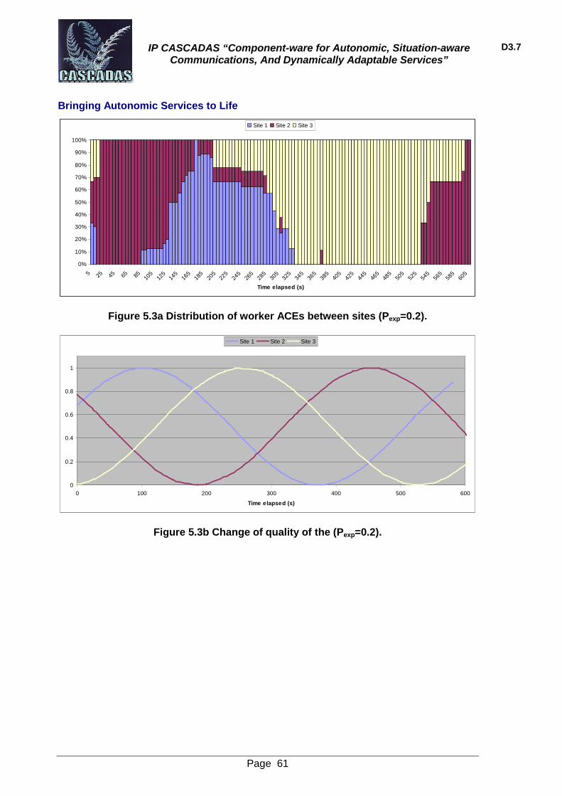
IP CASCADAS “Component-ware for Autonomic, Situation-aware Communications, And Dynamically Adaptable Services”
D3.7
Bringing Autonomic Services to Life
Page 61
0%
10%
20%
30%
40%
50%
60%
70%
80%
90%
100%
5 25 45 65 85 105
125
145
165
185
205
225
245
265
285
305
325
345
365
385
405
425
445
465
485
505
525
545
565
585
605
Time elapsed (s)
Site 1 Site 2 Site 3
Figure 5.3a Distribution of worker ACEs between sites (Pexp=0.2).
0
0.2
0.4
0.6
0.8
1
0 100 200 300 400 500 600
Time elapsed (s)
Site 1 Site 2 Site 3
Figure 5.3b Change of quality of the (Pexp=0.2).
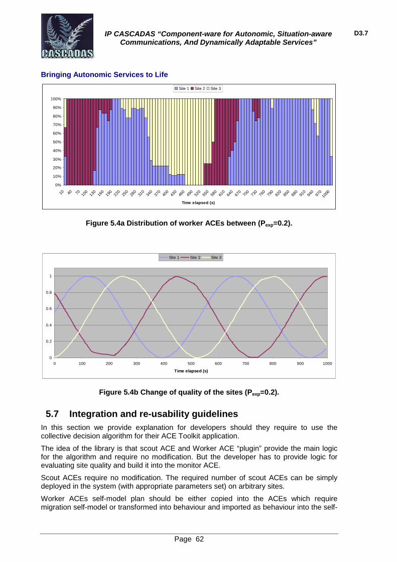
IP CASCADAS “Component-ware for Autonomic, Situation-aware Communications, And Dynamically Adaptable Services”
D3.7
Bringing Autonomic Services to Life
Page 62
0%
10%
20%
30%
40%
50%
60%
70%
80%
90%
100%
10 40 70 100
130
160
190
220
250
280
310
340
370
400
430
460
490
520
550
580
610
640
670
700
730
760
790
820
850
880
910
940
970
1000
Time elapsed (s)
Site 1 Site 2 Site 3
Figure 5.4a Distribution of worker ACEs between (Pexp=0.2).
0
0.2
0.4
0.6
0.8
1
0 100 200 300 400 500 600 700 800 900 1000
Time elapsed (s)
Site 1 Site 2 Site 3
Figure 5.4b Change of quality of the sites (Pexp=0.2).
5.7 Integration and re-usability guidelines In this section we provide explanation for developers should they require to use the collective decision algorithm for their ACE Toolkit application.
The idea of the library is that scout ACE and Worker ACE “plugin” provide the main logic for the algorithm and require no modification. But the developer has to provide logic for evaluating site quality and build it into the monitor ACE.
Scout ACEs require no modification. The required number of scout ACEs can be simply deployed in the system (with appropriate parameters set) on arbitrary sites.
Worker ACEs self-model plan should be either copied into the ACEs which require migration self-model or transformed into behaviour and imported as behaviour into the self-

IP CASCADAS “Component-ware for Autonomic, Situation-aware Communications, And Dynamically Adaptable Services”
D3.7
Bringing Autonomic Services to Life
Page 63
model. The will then automatically provide migration behaviour to the ACE (assuming the scout and monitor ACEs are deployed in the system).
Monitor ACE is the one that should be modified most by the developer because the provision of site information is application dependent. The ‘modifiable’ section is indicated in the example.swarmmigration.Monitor.sendSiteInformation() method. The SiteInformation interface has to be implemented by the developer providing implementation of compare(SiteInformation) method which should return the java.lang.Double value which should show how good the given SiteInformation is compared to itself. For example, if quality of S1 is 6 and quality of S2 is 3 so S1.compare(S2) should return 0.5, and S2.compare(S1) could return 2.0. This information will be used by scouts in determining their site preference. The site information should be added as “site_information” parameter to the ServiceResponseEvent sent to the scout.
6 Conclusion
The overarching conclusion that can be drawn from the examples compiled in this document is the plasticity and wide-range applicability of self-* design principles. The fact that algorithms that are in fact conceptually very close (i.e. featuring a random component, relying on large numbers of micro-events etc.) can be leveraged to identify and/or implement workable solutions to problems ranging from load-balancing to service migration and energy optimization is clear evidence of their almost ubiquitous usability.
Some of our results have nevertheless uncovered the practical hurdles that must sometimes be overcome in order to apply self-* design principles to the refinement and improvement (as opposed to the development “from scratch”) of real-world systems. In many cases, compromises have to be found with other engineering paradigms in order to achieve harmonious integration. Our experience suggests that this often requires considerable effort and that developing a sound methodology to facilitate this integration process should perhaps be considered as an explicit objective for future work.
From a scientific and technical point of view, the diversity of our findings offers many opportunities for further research. One example would be investigating the possibility that identifying optimal parameter values for local rules (e.g. individual threshold determining the ratio between rewiring and processing in the load-balancing scenario) might become part of the run-time self-organization process (as opposed to an offline exercise conducted prior to implementation). This would certainly enhance the ability of a system to adapt to changes in its execution environment, as it would eliminate the need for external updates, effectively replacing them with continuous self-training of individual components. However, as illustrated by some of our own results (e.g. the pathological emergent properties of the “passive” rewiring algorithm or the exponential duration of collective decision-making in some regions of the parameter space), this is an ambitious objective that would require very careful selection and design of the adaptation functionalities themselves.
With the “Green ICT” agenda gaining increasingly more momentum, another promising area for future work is the application of self-* distributed techniques to energy management, not only for own use by the ICT sector (as in the server farm example presented in this deliverable) but also for the general public. For instance, there are many indications that electricity generation and distribution is progressively being transformed from a completely centralized infrastructure (national grids) to one that could incorporate

IP CASCADAS “Component-ware for Autonomic, Situation-aware Communications, And Dynamically Adaptable Services”
D3.7
Bringing Autonomic Services to Life
Page 64
micro-generation and micro demand-side management. The explosion in the diversity of usage and production patterns that could result from such fundamental shift seems to provide an ideal area of application for self-* design.
Finally, systems science and the continuing study of the many examples of self-* design found in nature should not be neglected. Throughout this project, we have tried to maintain a balance between analytical modeling and simulation-based approaches, focusing respectively on understanding the fundamental dynamics of complex self-* systems and on adapting their governing principles to more or less idealized versions of technological problems. However, time constraints have sometimes prevented us from completely finalizing the link between the two sets of results and, maybe more importantly, from publishing what we consider to be important scientific findings in appropriate journals or conferences. For instance, at present, some results on the emergent topological properties of graphs produced by self-aggregation have only been presented in project deliverables. Similarly, the work on finalizing the collective decision-making models so as to identify their key properties (as opposed to informing the design of applicable local rules) is still ongoing. We expect at least 2 original papers on these WP3 results to be produced after the formal closure of the project.
7 References
[1] Barabasi, A.-L., & Reka, A. (1999). Emergence of Scaling in Random Networks. Science (286), 509-512.
[2] Chen, G., He, W., Liu, J., Nath, S., Rigas, L., Xiao, L., and Zhao, F. Energy-aware server provisioning and load dispatching for connection-intensive internet services. Tech. rep., Microsoft Research, 2008.
[3] Cybenko, G. (1989). Dynamic load balancing for distributed memory multiprocessors. Journal on Parallel and Distributed Computing , 7 (2), 279-301.
[4] Di Nitto, E., Dubois, D., & Mirandola, R. (2007). Self-Aggregation Algorithms for Autonomic Sysems. Bionetics '07. Budapest.
[5] Di Nitto, E., Dubois, D., Mirandola, R., Saffre, F., & Tateson, R. (2008). Applying Self-Aggregation to Load Balancing: Experimental Results. Bionetics '08. Awaji Island.
[6] Mailleux A. C., Detrain C. and Deneubourg J.L. (2003): “Regulation of ants’ foraging to resource productivity”. Proc. R. Soc. London B: 270, pp: 1609-1616
[7] Qian, X., & Yang, Q. (1994). An analytical model for load balancing on symmetric multiprocessor systems. Journal on Parallel and Distributed Computing , 20 (2), 198-211.
[8] Saffre F. and Blok H.R. (2005), “SelfService: A Theoretical Protocol for Autonomic Distribution of Services in P2P Communities” in Proceedings of the 12th IEEE International Conference and Workshops on Engineering of Computer-Based Systems, pp: 528 – 534
[9] Sanders, P. (1999). Analysis of nearest neighbor load balancing algorithms for random loads. Parallel Comput, 25(8), p. 1013-1033.
[10] WP3. (2006). Cascadas Deliverable D3.1.
[11] WP3. (2006). Cascadas Deliverable D3.2.
[12] WP3. (2007). Cascadas Deliverable D3.3.
[13] Xu, C.-Z., & Lau, F. C. (1995). The generalized dimension exchange method for load balancing in k-ary n-cubes and variants. Journal of Parallel and Distributed Computing , 24 (1), 72-85.